Evaluating effective income tax progression

ELSEVIER Journal of Public Economics 56 (1995) 461-474

JOURNAL OF PUBLIC ECONOMICS

Evaluating effective income tax progression

Kathy J. Hayes a, Peter J. Lambert b'*, Daniel J. Slottje a "Department of Economics, Southern Methodist University Dallas, TX 75275, USA

bDepartment of Economics, University of York, York, Y01 5DD, UK

Received May 1992, final version received November 1993

Abstract

An algorithm to compute effective income tax progression is devised for use when taxes are a function of both money income and other socioeconomic attributes and the data is in grouped (summary) form suppressing non-income information. Effective progression can be evaluated at percentiles in the distribution of either money or equivalent income. The normative significance of the new measures is explained in both cases. The methodology is illustrated by application to U.S. individual income tax annual data for 1950-1987, yielding contour plots which show how effective progression has varied across the income distribution and with the passage of time.

Key words: Progression; Progressivity; Welfare; Inequality; Redistribution

J E L classification: D63, H24

I . Introduct ion

I t is impor tan t for the assessment of the distr ibutional impact o f tax code changes to have a m e t h o d o l o g y for evaluat ing progress ion at different points in the income parade . Liability and residual progression, two normat ive ly significant measures of local progression, are defined by marginal and average tax rates for any tax code in which people ' s liabilities are de- t e rmined solely by their income levels. But in reality people ' s tax liabilities

* Corresponding author.

0047-2727/95/$09.50 (~) 1995 Elsevier Science B.V. All rights reserved SSDI 0047-2727(94)01429-R

462 K.J. Hayes et al. / Journal of Public Economics 56 (1995) 461-474

depend on non-income characteristics, such as marital status, age, home- ownership, interest rates, life insurance and charitable giving as well as on income. A methodology to take such differences in tax treatment explicitly into account in performing aggregate distributional analysis is lacking in the progressivity literature.

At the same time, the analyst all too often has to work with grouped data, provided in summary tabulated form and suppressing the tax-relevant non- income information. Then, of course, disaggregated analysis is imposs ib le- and the need for a well-founded aggregate procedure is the more pressing. In this paper we develop an algorithm to compute effective progression profiles, as defined shortly, from the information held in concentration and relative concentration (Suits) curves for taxes and post-tax incomes. The conventional practice of using group averages to compute effective progression is inherently deficient compared with the use of concentration curves; this will be shown inter alia in Section 2. The new algorithm, developed in Section 2, will reveal that the collapsing of concentration data into a scalar progressivity index itself constitutes an undue compression of information.

Minimal assumptions are made about the income tax in order to derive the algorithm. The tax code is modelled simply as a bundle of (say) n progressive income tax schedules, (tl(X), tz(X).. , t . (X ) ) where x is pre-tax income and ti(x), 1 <- i <- n, is tax liability, together with a rule for assigning income units to schedules. An income unit assigned to schedule ti(x) will be referred to as an income unit of type i. The single, the married, the old, the homeowners , the charitable givers, etcetera, may be recognized by the tax code to be of different types for income tax purposes, and hence assigned different schedules.

Given this minimal structure, the algorithm computes profiles K ( p ) and K * ( p ) , where p is rank in the pre-tax income parade, determining the liability and residual progression respectively at an income level, say y, ranked 100p% of the way up the pre-tax income parade, of the "averaged" schedule:

t(x) = ~iOi(x)ti(x) (1)

which expresses the mean tax paid by income units of all types at each pre-tax income x. Here Oi(x ) is the proportion of income units having income x which are of type i. Evaluation at percentiles rather than income levels permits the tracking of effective progression through time concurrent with a changing pre-tax income distribution. The technique can therefore be used, not only to assess the progressivity effects of tax code changes across the income parade, but also to reveal the effects on progressivity when the tax code is not undergoing adjustment but, rather, pre-tax incomes are growing or (for example) becoming more unequal.

K.J. Hayes et al. / Journal o f Public Economics 56 (1995) 461-474 463

The algor!thm is equally applicable to money income data and to equivalent income data, the ti(x ) in the latter case being interpreted as the taxes upon equivalent income x which are induced by the money income tax code. The normative significance of the profiles K ( p ) and K * ( p ) differs slightly in the two scenarios. This issue is addressed in Section 3. In common with other progressivity measures, K ( p ) and K * ( p ) describe the "vertical" effect of the income tax code; we show how additional information on the "hor izonta l" effects of departures [ti(x ) - t(x)] from the averaged schedule is needed fully to determine the inequality and welfare impacts. Other recent research is adduced to show the precise nature of these additional influences, and it is noted that microdata would be needed to quantify their impacts. At this point, we reach the limits of what is possible, given our self-imposed remit at the outset, to delineate a methodology for application to grouped data sets. Such data, which inextricably mingles socioeconomic, tax code and income distributional factors, cannot reveal the full welfare impact of an income tax code; but it can reveal much more than has here tofore been achieved by use of summary progressivity indices.

In Section 4, we apply the method to the U.S. distribution of money income and individual income tax, computing profiles for effective liability and residual progression annually from 1950 to 1987 using Statistics o f Income grouped data sets, and combining the resulting profiles into a pair of contour plots which show how each measure has varied across the income distribution and with the passage of time. Estimation problems are discussed here, modulo which our demonstration establishes the power of the approach not only to answer such topical questions as whether progression is more severe at the top or the bottom end of the distribution, but also, in the time dimension, whether income taxes are becoming more or less progressive, and for whom.

Section 5 concludes with the discussion, which places this paper in relation to the existing progressivity literature and reviews its achievements.

2. Concentration curves and effective progression

Let the distribution function and frequency density function for overall pre-tax income be F(x) and f (x) respectively. Liability progression at income level y of the "averaged" income tax schedule t(x) defined by equation (1) is the elasticity of tax to income:

L P ( y ) = e *~y)'y = y t ' ( y ) / t ( y ) (2a)

whilst residual progression is the elasticity of post-tax income:

R P ( y ) = e y-*~y)'y = y[1 - t ' ( y ) ] / [y - t(y)] (2b)


If p = F(y) ~ [0, 1], the income unit with income y has rank p in the pre-tax income parade. The Lorenz curve for pre-tax income, Lx(p), concentration curve for taxes, Lr(p) , and concentration curve for post-tax incomes, Lx_r (p ) , according to the averaged schedule t(x) are defined, as explained in Lamber t (1993a, chapter 2), which uses the same notation, by the following integrals:

Y t ~

Lx(p) = J xf(x) dx/tx (3a) 0

Y

LT(p) = J t(x)f(x) dx/Izt (3b)

g *

0

and: Y

Lx_v(p ) = f Ix - t(x)]f(x) dx//x(1 - t) 0

(3c)

where p~ is mean pre-tax income and t is the total tax ratio (fraction of total income taken in tax according to the averaged schedule t(x)).

The Suits (1977) curve for taxes (or relative concentration curve), Rr(q) say, plots cumulated portions of tax falling on various cumulated portions of pre-tax income. Thus if:

q = Lx(p ) (4)

then the Suits curve can be implicitly defined by:

R r ( q ) = Lr(p) (5a)

Similarly, a Suits curve for post-tax income, Rx_r(q) , can be defined as:

R x - T(q) = L x - T(P) (5b)

The slopes of all these concentration and relative concentration curves can be obtained by differentiation in (3) - (5) , as:

L~(p) = t(y)/l~t, R ~(q) = t(y)/ty (6a)

L'x -r (p) = [y - t(y)]/t~(1 - t), R ~ - r ( q ) = [y - t (y)]/( l - t)y (6b)

A more detailed exposition, and comparison of the Lorenz-based and Suits-based frameworks for tax analysis, is laid out in Lambert (1993a, chapter 7); see also Formby et al. (1981). As discussed in Basmann et al. (1992) in the case of the Lorenz curve, the curvatures of the concentration and relative concentration (Suits) curves of taxes depend significantly upon the frequency density of income units at each percentile point, as well as upon the averaged schedule t(x). In this paper we employ the novel

K.J. Hayes et al. / Journal of Public Economics 56 (1995) 461-474 465

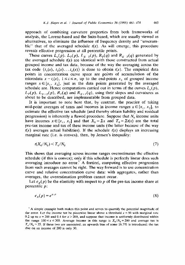
a p p r o a c h of combin ing curvature proper t ies f rom both f r ameworks of analysis, the Lorenz -based and the Suits-based, which are usually viewed as al ternat ives, to el iminate the influence of f requency density and "unsc ram- b le" that of the averaged schedule t(x). As will emerge , this p rocedure reveals effective progress ion at all percenti le points.

These curves Lx(p), LT(p) , Lx_r (p ) , R r ( q ) and Rx_r(q) genera ted by the averaged schedule t(x) are identical with those cons t ruc ted f rom actual g rouped income and tax data , because of the way the averaging across the tax code (tl(X), t 2 ( x ) . . . t , ( x ) ) is done to obtain t(x). The empirical data points in concen t ra t ion curve space are points of accumula t ion o f the mic roda ta x - ti(x ), 1 <-i <-n, up to the end-points x 2 of g rouped income ranges x ~ [x~, x2], just as the data points genera ted by the averaged schedule are. Hence computa t ions carr ied out in terms of the curves Lx(p), L r (p ) , L x _ r ( p ) , Rr (q) and Rx_r(q ) , using their slopes and curvatures as abou t to be described, are implementab le f rom grouped data.

It is impor tan t to no te here that, by contrast , the practice of taking mid-po in t averages o f taxes and incomes in income ranges x E Ix 1, x2], to es t imate the effective tax schedule (and thereby obtain liability and residual progress ion) is inherent ly a flawed procedure . Suppose that N O income units have incomes x E [x~, x2] and that X 0 = Ex and T O = Et(x) are the total pre- tax income and tax of these income units ( the latter because of the way t(x) averages actual liabilities). I f the schedule t(x) displays an increasing margina l rate (i.e. is convex) , then, by Jensen ' s inequality:

t(Xo/No) < To/N o (7)

This shows that averaging across income ranges overes t imates the effective schedule (if this is convex); only if this schedule is perfect ly linear does such averag ing in t roduce no error. 1 A f o r t i o r i , comput ing effective progress ion f r o m such averages cannot be right. The way forward is to use concent ra t ion curve and relative concent ra t ion curve data: with aggregates, ra ther than averages , the overes t imat ion p rob lem cannot occur.

Le t ex(p) be the elasticity with respect to p of the pre- tax income share at percent i le p :

ex(p) = e q'p (8)

1 A simple example both makes this point and serves to quantify the potential magnitude of the error. Let the income tax be piecewise linear above a threshold x = 50 with marginal rate 0.2 up to x = 200 and 0.4 for x > 200, and suppose that income is uniformly distributed within the range 100 <- x --- 300. Average income in this range is Xo/No=200 and average tax is To/N o = 35. If these two are associated, an upwards bias of some 16.7% is introduced: the tax due on an income of 200 is only 30.

466 K.J. Hayes et al. / Journal o f Public Economics 56 (1995) 461-474

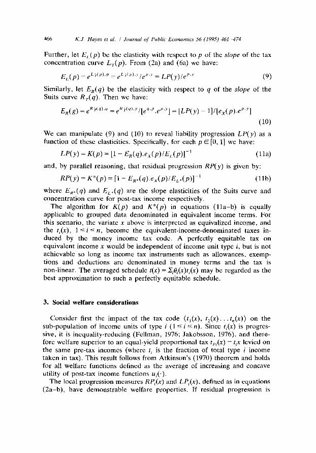
Further , let EL(p) be the elasticity with respect to p of the slope of the tax concentrat ion curve L r ( p ) . From (2a) and (6a) we have:

EL(p) = e LEp~'p = eL EP)'Y /e p'y = LP(y ) /e p'y (9)

Similarly, let ER(q) be the elasticity with respect to q of the slope of the Suits curve Rr (q) . Then we have:

E R ( g ) = e R~(q)'q = elC)~q)'Y /[eq'P.e p'y] = [LP(y) - 1]/[ex(p).e p'y]

( 1 0 )

We can manipulate (9) and (10) to reveal liability progression LP(y) as a function of these elasticities. Specifically, for each p E [0, 1] we have:

LP(y) = K(p) = [1 - En( q) .ex(p)/EL(p)] -~ ( l l a )

and, by parallel reasoning, that residual progression RP(y) is given by:

R P ( y ) = K*(p ) = [1 - ER.( q) .ex(p) / EL.(p)] -1 ( l l b )

where ER.(q ) and EL.(q ) are the slope elasticities of the Suits curve and concentrat ion curve for post-tax income respectively.

The algorithm for K(p) and K*(p) in equations ( l l a - b ) is equally applicable to grouped data denominated in equivalent income terms. For this scenario, the variate x above is interpreted as equivalized income, and the t~(x), 1 <-i <-n, become the equivalent-income-denominated taxes induced by the money income tax code. A perfectly equitable tax on equivalent income x would be independent of income unit type i, but is not achievable so long as income tax instruments such as allowances, exemp- tions and deductions are denominated in money terms and the tax is non-linear. The averaged schedule t(x) = XiOi(x)t~(x) may be regarded as the best approximation to such a perfectly equitable schedule.

3. Social welfare considerations

Consider first the impact of the tax code (tl(x), t2(X).., tn(x)) on the sub-population of income units of type i (1 -< i -< n). Since ti(x ) is progressive, it is inequality-reducing (Fellman, 1976; Jakobsson, 1976), and therefore welfare superior to an equal-yield proportional tax tpi(X ) = tix levied on the same pre-tax incomes (where t~ is the fraction of total type i income taken in tax). This result follows from Atkinson's (1970) theorem and holds for all welfare functions defined as the average of increasing and concave utility of post-tax income functions ui(. ).

The local progression measures RPi(x ) and LPi(x), defined as in equations (2a-b) , have demonstrable welfare properties. If residual progression is


increased, by reducing RPi(x ) at all income levels, post-tax inequality falls (Jakobsson, 1976); if this reform is revenue-neutral or revenue-reducing, welfare is enhanced. If residual progression is reduced, revenue-neutrally or with a revenue increase, welfare falls. Although not stressed by Jakobsson, similar properties hold for liability progression: if LPi(x) is increased at all income levels, revenue-neutrally (or even with an increase in revenue), post-tax inequality falls, with welfare enhancement in the revenue-neutral case, whilst if LP~(x) is reduced, revenue-neutrally or with a revenue decrease, inequality rises, with a fall in welfare in the revenue-neutral case [Lambert (1993a), exercise 7.2.2(a)]. There are also determinate inequality and welfare effects following upon liability and residual progression neutral changes in the schedule ti(x ) (Pffihler, 1984; Formby et al., 1992).

The welfare impact of the overall tax code is more difficult to determine at the level of generality maintained in this paper, but the effective progression measures K(p) and K*(p) can be linked with welfare as follows.

First, in case the variate x is money income, let (ul( . ) , u2(- ) . . , un(.)) be a bundle of utility of post-tax income functions satisfying Atkinson and Bourguignon's (1987) conditions for systematic differences in need between the different income unit types. Each u~(.) is increasing and concave, and marginal utilities and their differences are ranked in the same way at all income levels, reflecting a hierarchy of needs or social merit which is presumed also to rationalize differences in treatment in the tax code. Let overall welfare be average utility according to the bundle (u l(. ), u 2 ( . ) . . , un(-)). As shown in Lambert (1993b), the tax code is unambiguously welfare-superior to the equal-yield proportional tax re(x)= t.x on all pre-tax incomes regardless of type only if overall inequality in money income across types is unambiguously reduced. A necessary condition for this is that:

JR > 0 (12)

where IR denotes the reduction in inequality caused by the tax code as measured by the Gini coefficient.

Second, when the variate x is equivalized income, an index specification of welfare developed by Sen (1973) and others may appropriate. This depends only on the mean m and Gini coefficient G of the distribution in question:

W = m(1 - G) (13)

The rationale for Sen's formulation rests on pairwise income comparisons. Clearly a process of equivalizing would take place before, say, a single person tax unit and a family with three children would make such a comparison. Comparing the welfare impact of the actual tax code with that


of a proportional tax yielding the same revenue (this time denominated in units of equivalent income), we have:

WX-T--Wx e = m [ G x - G x T]=m'IR (14)

where m is mean post-tax equivalent income and G x and G x r are the pre- and post-tax Gini coefficients. Again condition (12), IR > 0 , is necessary (and in this case also sufficient) for the tax code to be welfare-superior to flat tax levied regardless of type.

The significance of the effective progression measures K(p) and K*(p) is that they partly determine the inequality effect IR of the tax code. In Aronson et al. (1994) it is shown that the inequality reduction caused by the averaged schedule t(x) can be isolated from that which is caused by departures [ti(x ) - t ( x ) ] from it, and that these departures themselves contribute two influences to IR, attributable to (i) the unequal treatment of pre-tax "equals" (those having the same income x but being of different types), and (ii) the reranking which is induced between pre-tax "unequals":

/R = [t/(1 - t )] .P- H - R (15)

Here, t is the total tax ratio (as before); P is the Kakwani (1977a) index of progressivity which would obtain if, counterfactually, every tax unit had paid tax according to the averaged schedule t(x) instead of the type-specific schedule ti(x); R is the index due to Atkinson (1980) and Plotnick (1981) which captures the effect on inequality of rank reversals in the transition from the pre- to post-tax income parade; and H is a measure of unequal tax treatment which is defined as follows. Denote by Gx_r(x ) the Gini coefficient for post-tax income among all those having pre-tax income x (of all types), and let a(x) be the product of the population share and post-tax income share of these tax units. Then:

H = (16)

which is an aggregate measure of the unequal tax treatment of "equals". As shown in Kakwani (1977b), the description index P, which quantifies

the extent to which averaged taxes deviate from proportionality, goes up if liability progression K(p) is increased at all percentiles, whilst the whole term [ t / ( 1 - t ) ] . P in (15), an index of redistributive effect, goes up if effective residual progression is enhanced (that is, if K*(p) is reduced). These terms go towards the determination of the inequality impact IR of the tax code (and hence the welfare effect), and constitute the only positive influences; this establishes the normative significance of K(p) and K*(p). The two further inputs - H and - R , stemming from departures from the averaged schedule (differences in tax treatment), are negative, being effects


which act to counteract the vertical impact of the averaged schedule. Requi rement (12) can, of course, alternatively be written as:

[t/(1 - t )] .P> H + R (17)

showing that, for welfare superiority over flat tax, the vertical effect of the averaged schedule (with inputs K(p) and K*(p)) must outweigh the horizontal and reranking effects.

The profiles K(p)and K*(p) reveal significantly more about vertical incidence than do the indices P and [ t / ( 1 - t ) ] . P , which compress the available information until sight is lost of differential effects. Of the two other effects, - H could only be determined from microdata (consider (16)), whereas - R may be estimated from grouped data if this is presented by both range of pre-tax income and range of post-tax income; at this point we reach the limit of what is feasible given only grouped data.

4. Effective progression in the United States

The measures K(p) and K*(p) are easily derivable from income and tax data which is published in grouped (summary) form, whether the data is denominated in money or equivalent income terms. Evaluation at percentiles rather than income levels permits the tracking of effective progression through time, concurrent with a changing pre-tax income distribution, or indeed its comparison among taxing jurisdictions. Whilst microdata is clearly superior for this sort of analysis, offering scope to unscramble the influences of tax code changes/differences from those of demographics and distribution, the profiles derived from grouped data clearly bring out more than conventional indices.

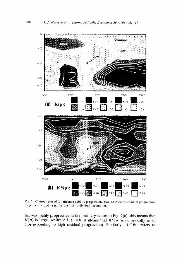
In the U.K. , summary tabulations to show the impact of the personal income tax have been presented in equivalent terms, in Economic Trends, only since 1990. Whilst the equivalent income scenario is perhaps of more interest, we opted rather for the long series of summary tabulations available from 1950 for the U.S. individual income tax in Statistics of Income, in which the data is given in money terms, to illustrate the potential of our approach. By computing income and tax shares, concentration and Suits curve slopes and arc elasticities from this data, we obtained 38 annual profiles for each measure of effective progression using formulae (11a-b). These profiles are fully specified in Hayes et al. (1991), and are summarized in Fig. 1 as a pair of contour plots. These show how liability and residual progression have varied across the (money) income distribution and with the passage of time. We mark as " H I G H " , in these plots, regions in which the


0 ;5

90

i l l

Or~;

I t70

I l l

LOW

9BO i 987

8! ~ I 73 ; 56

~ i 3 0 D ' 2 3

II

~. 75

) 5('s

o 25

i3 ~0

(b) Q 9 i l 093 ~ O~

Fig. 1. Contour plot of (a) effective liability progression, and (b) effective residual progression, by percentile and year, for the U.S. individual income tax.

tax was highly progressive in the ordinary sense: in Fig. l(a), this means that K(p) is large, whilst in Fig. l (b) it means that K*(p) is numerically small (corresponding to high residual progression). Similarly, "LOW" refers to


regions (deciles and years) in which the tax was at its least progressive in the ordinary sense.

The profiles are, of course, estimates of progression in the U.S. population at large, and when compared between years sampling errors reduce precision. Even for a fixed year, when the profile can be regarded as a population rather than sample statistic (the annual sub-population of tax returns upon which Statistics of Income is based is quite large), bias arises from the grouping which has taken place, and precision is reduced. Modulo these difficulties, a notable conclusion is that at no point in time was either profile, K(p) or K*(p) , unambiguously dominant; there is no "outl ier" year. The changes which have taken place in these profiles can, of course, be attributed to periodic tax reform (Davis, 1986; Bakija and Steuerle, 1992) and, in between times, to pre-tax distributional and demographic change. A general pattern is of increasing progression through time, arrested by periodic tax reform. This pattern will, of course, be reflected in the indices [ t / ( 1 - t)].P and P discussed in Section 3. Similar trends were detected by Fries et al. (1982) in respect of revenue elasticity for the shorter period 1963-1977. An explanation for both phenomena is in terms of the inflation tax: reform acts as a partial indexing device, ameliorating bracket- creep and restoring the income tax in real terms. Liability progression and residual progression do not necessarily move together as income varies, as is well-appreciated: in all years, progression is less at the very top of the distribution than near the bottom in terms of liability progression (as quantified by K(p)), but the opposite is generally true (higher progression at the top) in terms of residual progression (K*(p) numerically low at the top). Two regions of high progression in both senses are the first decile in the early 1960s, and the third decile in the early 1980s. The first effects of the 1986 Tax Reform Act show reduced progression in the 3rd to 8th deciles, but slightly increased progression at both ends according to both measures, and this confirms Musgrave's (1987) simulations (ibid., page 65).

5. Discussion

Broad-brush conclusions such as those indicated above are hardly access- ible using global progressivity indices. They are, of course, subject to sampling error qualifications, in common with conclusions drawn from indices.

Almost all constructions in the income tax progressivity literature are founded upon the assumption that a common tax schedule t(x) faces all income units. Indeed, consistency with liability or residual progression of this underlying schedule has been the organizing principle for the index measurement of progressivity since the pathbreaking work of Suits and


Kakwani (Lambert, 1993a, chapter 7). In a more recent development, Pfingsten (1986) goes further, demanding of his index, in addition to consistency with residual income progression, the property that: "if the local degree of progression is the same for all households, then it should be equal to the global progressivity" (ibid., page 84). The multi-valued measures K(p) and K*(p) of effective progression along the income parade enjoy a similar but more powerful design feature, which we might re-phrase thus; "if the tax schedule is the same for all households, then its local degree of progression is equal to the effective progression at each percentile".

The starting point in this paper was a tax code (tl(X), t2(x) . . . tn(x)) , rather than a schedule, but the profiles K(p) and K*(p) relate only to the (vertical) impact of the averaged schedule t(x) = ~Oi(x)ti(x ). Ceteris paribus, upward/downward shifts of these profiles, secured by reform of the component schedules ti(x), would have inequality and welfare impacts through the first term in equation (15), but tax code changes also have implications for the (horizontal) contributions to (15). These effects cannot be revealed from grouped data, and hence are outside our remit.

Only one other study, that of Kakwani (1984), allows for differences in tax treatment, but the income tax is not modelled explicitly. An index decomposition of IR resembling (15):

IR = [t/(1 - t)l.P T - R (18)

arises in this study, where Pr is a concentration-based progressivity index, but there are no proven links between Pr and the component schedules t~(x) of a tax code (tl(X), t2(x)...t,,(x)). By separating out the additional horizontal effect - H of unequal treatment of pre-tax "equals" from It/(1 - t)].P r in (18), links between effective progression K(p) and K*(p) and the indices P and It/(1 - t ) ] . P of (15) are established. In turn, changes in local progression LPi(x ) and RP~(x) of the component schedules ti(x), which are ultimately the tax instruments, have explicit implications for effective progression. If, as before, income y is at percentile p, then:

K(p) = LP(y) = ~i[Og(y)t,(y)/t(y)].[~(y) + LP~(y)] (19)

where q~i(x) is the elasticity of Oi(x ) with respect to x. A similar relationship holds between K*(p) and the component RPi(y)'s. Recalling that Oi(x ) is the proportion of income units having income x which are of type i, demographics enter into the determination of q~i(x): in particular, ~(x) will be negative above the modal type i income. Together, (15) and (19) offer a constructive means to classify tax (reform) effects into the vertical and the horizontal, and this is a convenient organizing principle. In the equivalent income scenario, the effects - H and - R in (15) both measure inequities, the former relating to the unequal treatment of equals (classical horizontal

K.J. Hayes et al. / Journal o f Public Economics 56 (1995) 461-474 473

inequity) and the latter to reranking, an effect between unequals which has been argued to measure horizontal inequity (Feldstein, 1976). 2

Acknowledgements

The authors are especially appreciative of the helpful suggestions provided by an anonymous referee, and for comments on earlier drafts from John Formby, Stephen Jenkins, Tony Shorrocks and Joel Slemrod.

References

Aronson, J.R., P. Johnson and P.J. Lambert, 1994, Redistributive effect and unequal income tax treatment, Economic Journal 104 (forthcoming), 262-270.

Atkinson, A.B., 1970, On the measurement of inequality, Journal of Economic Theory 2, 244-263.

Atkinson, A.B., 1980, Horizontal equity and the distribution of the tax burden, in: H.J. Aaron and M.J. Boskins, eds., The economics of taxation (Brookings Institution, Washington D.C.) 3-18.

Atkinson, A.B. and F. Bourguignon, 1987, Income distribution and differences in needs, in: G.R. Feiwel, ed., Arrow and the foundations of the theory of economic policy (Macmillan, London) 350-370.

Bakija, J. and E. Steuerle, 1992, Individual income taxation since 1948, National Tax Journal 46, 451-475.

Basmann, R.J., K.J. Hayes and D.J. Slottje, 1991, The Lorenz curve and the mobility function, Economics Letters 35, 105-111.

Broome, J., 1989, What's the good of inequality? in: J.D. Hey, ed., Current issues in microeconomics (Macmillan, London) 236-262.

Davis, D., 1986, United States taxes and tax policy (Cambridge University Press, Cambridge). Economic Trends, monthly, Central Statistical Office (HMSO: London). Feldstein, M., 1976, On the theory of tax reform, Journal of Public Economics 6, 77-104. Fellman, J., 1976, The effect of transformations on Lorenz curves, Econometrica 44, 823-824. Formby, J.P., T.G. Seaks and W.J. Smith, 1981, A comparison of two new measures of tax

progressivity, Economic Journal 91, 1015-1019. Formby, J.P., W.J. Smith and P.D. Thistle, 1992, On the definition of tax neutrality:

distributional and welfare implications of policy alternatives, Public Finance Quarterly 20, 3-23.

Fries, A., J.P. Hutton and P.J. Lambert, 1982, The elasticity of the U.S. individual income tax: its calculation, determinants and behaviour. Review of Economics and Statistics 64, 147-151.

2 There would not be a reranking contribution to IR if this were to be measured using a decomposable (generalized entropy) inequality index rather than the Gini (Lambert and Aronson, 1993). The welfare irrelevance of ranking would arise because, whilst the Gini captures the unfairness of inequality, entropy indices essentially capture the wastefulness of it, which rank changes do not bear upon (Broome, 1989).


Hayes, K.J., D.J. Slottje and P.J. Lambert, 1991, Measuring effective tax progression, Economics Discussion Paper No. 9116, Southern Methodist University, Dallas, Texas.

Jakobsson, U., 1976, On the measurement of the degree of progression, Journal of Public Economics 5, 161-168.

Kakwani, N.C., 1977a, Measurement of tax progressivity: an international comparison, Economic Journal 87, 71-80.

Kakwani, N.C., 1977b, Applications of Lorenz curves in economic analysis, Econometrica 45, 719-727.

Kakwani, N.C., 1984, On the measurement of tax progressivity and redistributive effect of taxes with applications to horizontal and vertical equity, Advances in Econometrics 3, 149-168.

Lambert, P.J., 1993a, The distribution and redistribution of income: a mathematical analysis, second edition (Manchester University Press, Manchester).

Lambert, P.J., 1993b, Redistribution through the income tax, in: J. Creedy, ed., Taxation, poverty and income distribution (Edward Elgar, Aldershot) 1-16.

Lambert, P.J. and J.R. Aronson, 1993, Inequality decomposition analysis and the Gini coefficient revisited, Economic Journal 103, 1221-1227.

Musgrave, R.A., 1987, Short of euphoria, Journal of Economic Perspectives 1(1), 59-71. Pffihler, W., 1984, 'Linear' income tax cuts: distributional effects, social preferences and

revenue elasticities, Journal of Public Economics 24, 381-388. Pfingsten, A., 1986, The measurement of tax progression, Studies in Contemporary Economics

20 (Springer-Verlag, Berlin). Plotnick, R., 1981, A new measure of horizontal inequity, Review of Economics and Statistics

63, 283-288. Sen, A., 1973, On economic inequality (Clarendon Press, Oxford). Statistics of Income: Individual Income Tax Returns, annually (IRS: Washington D.C.). Suits, D., 1977, Measurement of tax progressivity, American Economic Review 67, 747-752.

Documents

Evaluating effective income tax progression