1

Evaluating Innovative Technologies for Multistage Fish Growth

Processes: a Case of an Eel Farm

Gregory Yom Din

Zinaida Zugman

Gad Degani

Gregory Yom Din, Golan Research Institute, University of Haifa, P.O.B. 97, Katzrin,

12900, Israel.

Zinaida Zugman, Golan Research Institute, University of Haifa, P.O.B. 97, Katzrin,

12900, Israel.

Gad Degani, Faculty of Civil and Environmental Engineering, Technion – Israel

Institute of Technology, Haifa 32000, Israel.

Running title: Evaluating Innovative Technologies

Correspondence Gregory Yom Din, Golan Research Institute, University of Haifa, P.O.B.

97, Katzrin, 12900, Israel. Tel.: 972-4-696-1330. Fax: 972-4-696-1930. Email:

rres102@research.haifa.ac.il

2

Abstract

The economic benefits of implementing innovative technologies at farm level are evaluated

when the technology includes multiple research lines at various intensities and several growth

stages. Data are presented in “bio-economic” tables that take into account the biological

parameters of each research line and the costs related to its development and implementation.

The adjusted data are then divided into groups of research lines, and feasible combinations of

lines for all three growth stages are evaluated to choose the best technology for the whole

growth process. Results reveal the most profitable research lines, detailed by growth stage

and intensity, for the 5-year eel culture. Comparison of the ten best technologies shows that

the technologies with the highest profits for single growth stages do not necessarily result in

the most additional profit for the farm.

Keywords: Innovative technology, fish farming, research benefits, research lines, bio-

economic tables

INTRODUCTION

This study was motivated by the need of researchers at MIGAL Laboratories (Galilee

Technological Center, Israel) to economically evaluate individual research lines in a

technology involving multiple research lines for eel farming. While a farmer’s sole criterion

for evaluating innovations may be profit, researchers are often interested in how changes in a

specific factor affect a total technology. Often, several research lines are studied

simultaneously. To determine the best complex of innovations, R&D decision-makers need

economically sound tools to evaluate the benefits of each research line.

Economic evaluations, especially in aquaculture, can be made either ex-ante or ex-

post experiment and/or according to level of modeling and implementation (industry or farm

level). The distribution of research benefits among farmers, processors, and consumers was

3

studied by Alston et al. (1999) who considered changes in demand and supply resulting from

changes in prices after implementation of an innovative technology. Their approach reveals

tendencies resulting from given economic assumptions about an industry and/or country.

According to Ekboir (2003), reliable results can be obtained at this level only post evaluation

of research benefits. Periods of 5-10 years of research implementation were used for post

evaluation in Carberry et al. (2002) and Dasgupta and Engle (2000).

Farm level modeling has also been used in studies for ex-ante economic evaluation of

innovative technologies. Dey (2000) used ex-ante evaluation of the impact of innovative

technologies for Nile tilapia in Asia, where results of on-farm trials were incorporated into

the fish sector model for the country. Jolly et al. (2004) used farm budgets and a linear

programming model for ex-ante evaluation of the returns to catfish hybrid research. Farm

level economic models are studied in Pannell (1999). The author discusses how a formal

research evaluation can improve research design. The latter can result in benefits for

researchers, particularly, by culling relatively unbeneficial research and redirecting funds to

relatively beneficial research.

Important features of farm level modeling are the use of bio-economic models and

taking into account multiple innovations. Economic models of fish farming take into account

technological constraints and bio-economic indices such as fish density, feeding (Dasgupta

and Engle 2000), survival rate (Valderrama and Engle 2004), water use, spawning, hatching

(Engle et al. 2000), size stocking, and optimal growing season (Webster 2004). Bio-economic

models can present changes of fish biomass as a non-linear function of fish growth and

survival rate for a wide range of farm scales (Gasca-Leyva et al. 2002). Models of fish

growth (Bolte et al. 2000) describe dynamics of fish livestock. A model of a discus farm

(Yom Din et al. 2002) deals with fish of different ages and sizes for a 5-year period. Dekker

(2000) developed an eel growth model for wild eels that was used for farmed eels by Frost et

4

al. (2001). A bio-economic model of eels was suggested in the study of De Leo and Gatto

(2001). Incorporating bio-economic models into evaluations of innovations on the farm level

adds causality to the description of complex systems such as aquaculture farms.

Innovative technologies for fish farming often include multiple lines of research,

especially in eel farming that consists of three growth stages. A model for evaluating the

costs of multiple research lines was developed by Sunding and Zilberman (2001). Their

model was modified by Yom Din et al. (2004) to evaluate the benefit of each research line

and the distribution of the benefit between researchers and farmers. The modified model

enables assessing how the benefits of each research line would change with changes in

parameters such as water temperature and turnover, hormone concentration, stocking density,

or diet.

The aim of our study was to develop a method for evaluating the benefits of

implementing technologies with multiple research lines based on the model of Sunding and

Zilberman, modified and adapted to the conditions of eel farms. In this study, financial

benefits were considered for both the farmer and the research team. The mechanisms of

receiving financial benefits in the organizations where the research team is "hosted" were

beyond the scope of this study and depend on country laws. An analysis can be found in

Rubin et al. (2003) for six countries: the USA, Britain, China, Japan, Germany, and Israel.

To our knowledge, the presented study is the first attempt to evaluate innovative

technologies with multiple research lines in fish farming research.

Eel farms involve three growth stages: glass eels are collected from the wild and kept

in small containers for three months; elvers are maintained for another nine months; and

yellow eels are raised to market size during the following 1.5-5 years. The most difficult

stage is the first three months after capture of glass eels. This period is characterized by high

mortality and a wide distribution of fish sizes (Degani and Levanon 1983). Metamorphosis

5

from unpigmented (glass) elvers to pigmented elvers involves morphological, physiological,

and behavioral changes. After metamorphosis, elvers are transferred to small ponds (Degani

and Levanon 1984) where they receive a special diet, steroids, and hormones. High-density

artificial conditions result in a high percentage of males (Kushnirov and Degani 1991). The

eels are transferred to large ponds during the third stage, where gender control and

manipulation are very important since females can reach 1000 g while male growth stops at

200-250 g.

MATERIALS AND METHODS

Data Collection

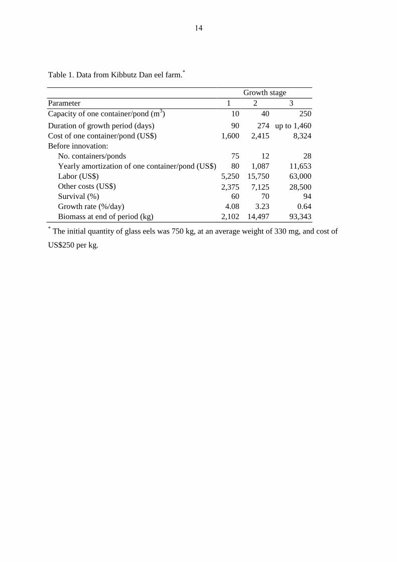
Data were taken from the model eel farm at Kibbutz Dan Fisheries (Table 1) and from

studies on water quality and temperature, fish density, diet, and hormones conducted at the

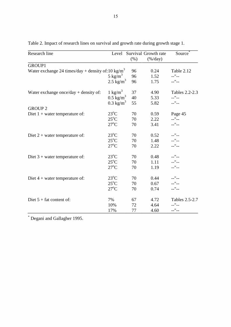
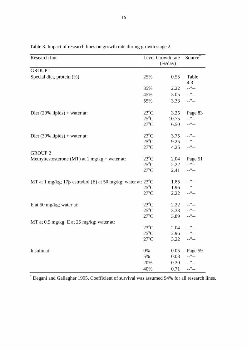
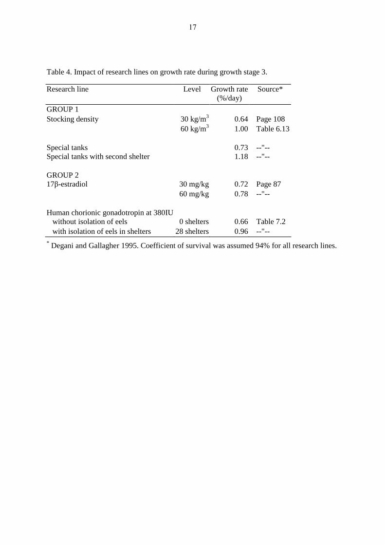
MIGAL Laboratories (Tables 2-4; Degani and Gallagher 1995). The number of research lines

for each stage was 9-26 with several levels of intensity (e.g., water temperatures, fish

densities, hormone doses). It was assumed that research lines for every stage can be divided

into two groups in such way that any line from the first group can be combined with any line

from the second group (a “feasible” combination of research lines). For example, a

combination of “water exchange 24 times per day with density of 10 kg/m3” and “diet 1 with

water temperature of 23°C” for the first stage of growth (Table 2) is a feasible combination.

Thus, innovative technologies comprised feasible combinations of two research lines for each

of the three growth stages. Thus, the number of considered research lines at different levels of

intensity was 6 and 15 for the first growth stage (Table 2), 10 and 16 for the second stage

(Table 3), and 4 and 4 for the third stage (Table 4) and the overall number of potential

6

innovative technologies for the studied case was estimated as 6 x 15 x 10 x 16 x 4 x 4 =

230,400.

Checking our Assumptions

In order to find a method for choosing the optimal combination of research lines, we

kept two factors in mind: (1) research lines are typically studied at only a few intensities,

therefore “optimal technology” as used hereinafter means “close to optimal technology”, and

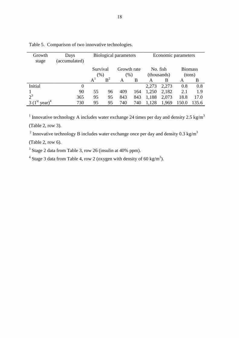
(2) the optimal technology does not necessarily include all the best-performing research lines.

To illustrate the latter assumption, we compared biomass after the third growth stage using

different research lines for the first stage and the same research lines for the second and third

stages in Table 5. In this comparison, technology A resulted in a better growth rate and

technology B in better survival in the first growth stage but technology A led to greater

biomass at the end of stage 3. Theoretically, if one could double the growth rate in the first

stage for technology B, the results would differ. Such an improvement in growth could be

achieved by using an additional research line during stage 1, for example, diet 1 with water of

27oC. Combining research lines within each stage and for all stages could produce results

unpredictable without using a proper quantitative method. Further, in addition to the results

of the research lines, the cost of inputs and research benefits should be taken into account.

We used the mathematical model (Yom Din et al. 2004) to evaluate implementation

of feasible innovative technologies.

Modification of the Input Data

Because of the complexity of the problem, data were presented in a format that

7

accounts for both the biological parameters of the research lines and the costs involved with

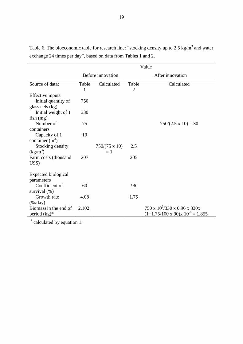
its development and implementation. Modified data were presented in “bio-economic tables”

that include: (1) costs of inputs of research lines, (2) farm costs, and (3) expected biological

parameters for each research line. As an example, the bio-economic table created for the first

period of eel growth is showed in Table 6.

Calculation Method

After preparing the bio-economic tables, the innovative technologies were

enumerated. First, we designed each technology to include two research lines for each stage:

one line from each group of research lines (Tables 2-4). The biological parameter (coefficient

of survival, growth rate - Table 6) resulting from the combination of the two research lines

was assumed as the geometric average, i.e., the root square of the value received after

multiplying the biological parameters of both research lines.

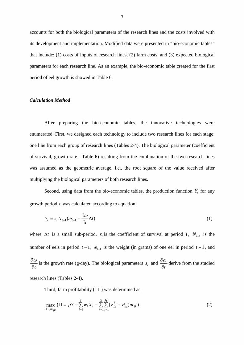
Second, using data from the bio-economic tables, the production function tY for any

growth period t was calculated according to equation:

)( 11 tt

NsY tttt ∆∂∂

+= −−ω

ω (1)

where t∆ is a small sub-period, ts is the coefficient of survival at period t , 1−tN is the

number of eels in period 1−t , 1−tω is the weight (in grams) of one eel in period 1−t , and

t∂∂ω

is the growth rate (g/day). The biological parameters ts and t∂

∂ωderive from the studied

research lines (Tables 2-4).

Third, farm profitability (Π ) was determined as:

))((max3

1 11,∑∑∑= ==

+−−≡Πk

kJ

jjk

rjk

fjk

I

iii

jkmiXmvvXwpY (2)

8

where p is the selling price, iw is the input price, iX is the value of input i , jkm is

intensity of thej th research line at stage k , fjkv is the farm’s expenses related to one unit of

line jk , and rjkv is the unit price of linejk that serves as a source of profit for the research

team. The term fjkv multiplied by intensity gives the additional expenses of the farm related

to the innovation (calculated from farm data in Table 1 and characteristics of the research

lines in Tables 2-4).

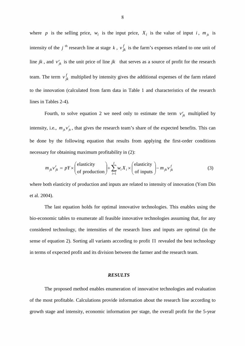
Fourth, to solve equation 2 we need only to estimate the term rjkv multiplied by

intensity, i.e., rjkjk vm , that gives the research team’s share of the expected benefits. This can

be done by the following equation that results from applying the first-order conditions

necessary for obtaining maximum profitability in (2):

fjkjk

I

iii

rjkjk vmXwpYvm −

×+

×= ∑

=1 inputs of

elasticity

production of

elasticity (3)

where both elasticity of production and inputs are related to intensity of innovation (Yom Din

et al. 2004).

The last equation holds for optimal innovative technologies. This enables using the

bio-economic tables to enumerate all feasible innovative technologies assuming that, for any

considered technology, the intensities of the research lines and inputs are optimal (in the

sense of equation 2). Sorting all variants according to profit Π revealed the best technology

in terms of expected profit and its division between the farmer and the research team.

RESULTS

The proposed method enables enumeration of innovative technologies and evaluation

of the most profitable. Calculations provide information about the research line according to

growth stage and intensity, economic information per stage, the overall profit for the 5-year

9

eel culture cycle, and the division of profit between the farmer and the research team, should

the given technology be implemented.

Based on this method, a computer program was created. The numerical decisions

enable determining which research lines should be included in the best technologies, the

amount of additional farm profit that can be expected after implementing the technology, and

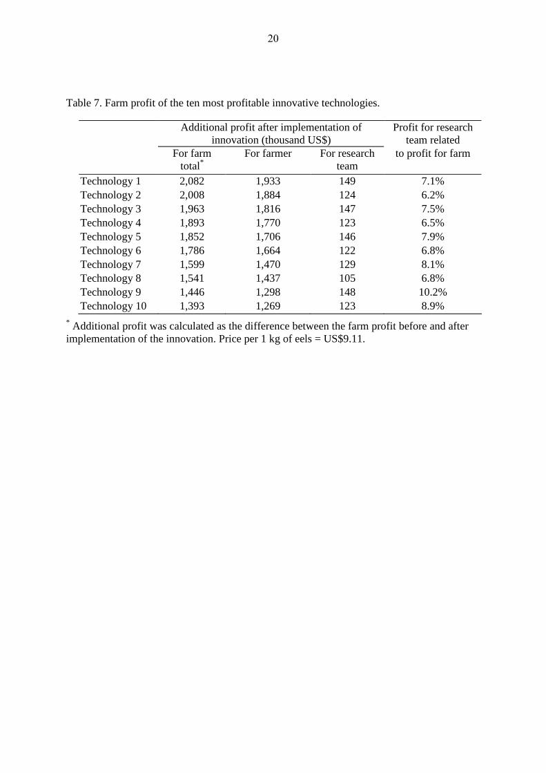
how the profit would be distributed between the researcher and the farmer. Table 7 shows

that the technologies with the highest profits for the research team do not necessarily result in

the most additional profit for the farm.

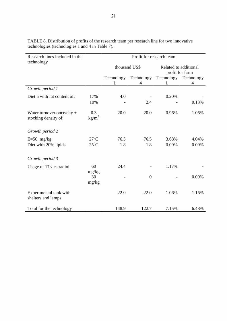
Every evaluated technology consisted of six research lines (one line for each group in

each growth stage, Tables 2-4). The distribution of benefits for two of the best technologies

(numbers 1 and 4; Table 7) is presented in Table 8. The differences between the two

technologies were the intensity of diet 5 in growth stage 1 and the dose of 17β -estradiol in

growth stage 3. The profit for the research team was divided in Table 8 by research lines and

growth stages according to equation 3 (which calculates the j th research line at stage k ).

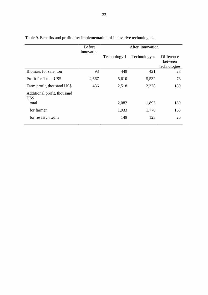
The differences between the technologies account for a difference in additional farm

profits of US$189,000 (Table 9). The profit for technology 4 was US$78 per ton less than for

technology 1. Technology 4 produced 28 tons less than technology 1. Therefore, technology

4 produced US$163,000 less for the farmer and US$26,000 less for the researcher.

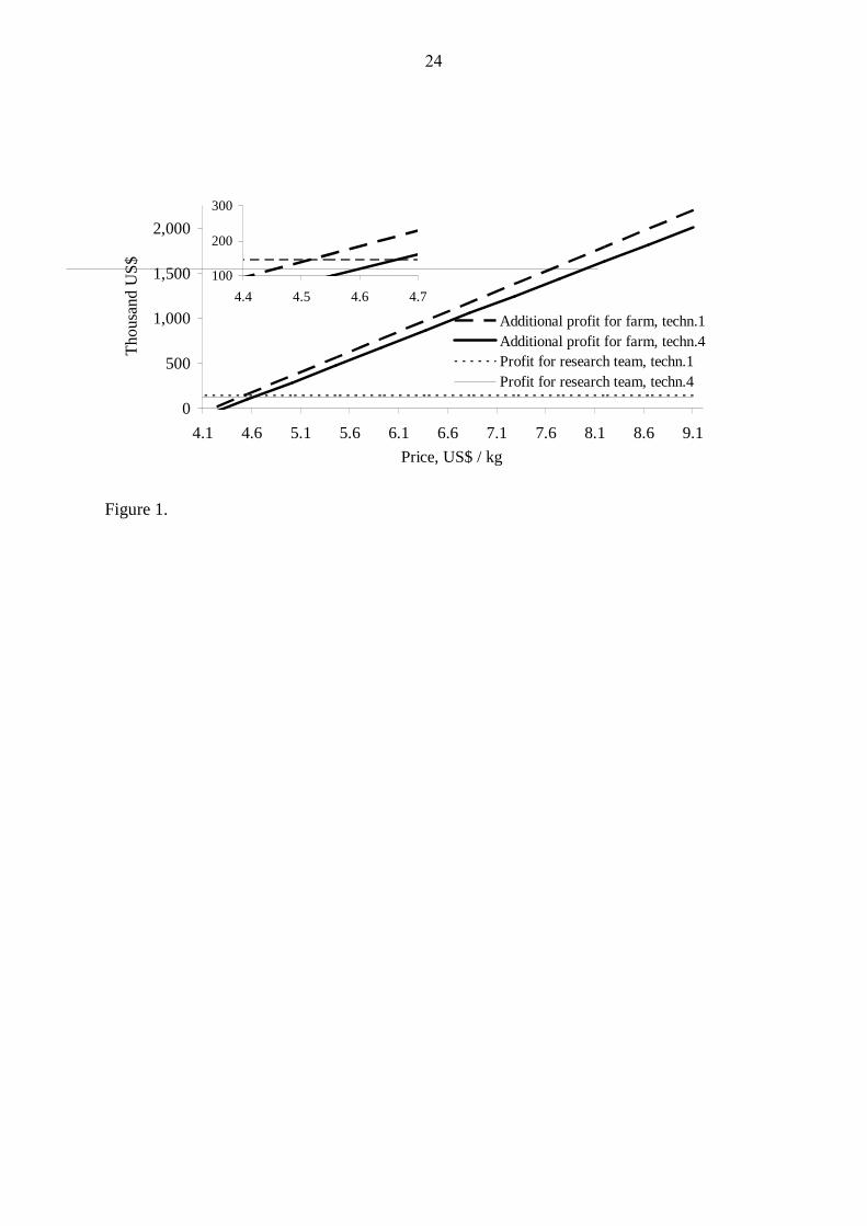
As eel prices decrease, the additional profit of the farmer that can be obtained after

implementing innovative technologies also decreases (Fig. 1). At some point, implementation

of the innovative technology is not recommended.

CONCLUSIONS

This paper presents a method to quantitatively evaluate in advance the expected

benefits of implementing new technologies at farm level. The method was designed

10

especially for cases in which innovative technologies include multiple lines of research. It is

therefore relevant to eel culture, which involves three growth stages during which different

conditions and technologies are required. The method enables choosing the best (optimal)

technology from numerous combinations of research lines by anticipating the additional

profit to be derived from implementing the technology. The best technology does not

necessarily include all the best-performing research lines. The method involves building bio-

economic tables from data on initial farm production and research results. The tables contain

information on (1) inputs, (2) farm costs, and (3) expected biological parameters for each

research line. Using this model helps to decide which technologies are likely to be winners.

Additional profit for the farm is differentiated for research lines and growth stages.

REFERENCES

Alston, J. M., R. J. Sexton, and M. Zhang. (1999) Imperfect competition, functional

forms, and the size and distribution of research benefits. Agricultural

Economics, 21,155-172.

Bolte, J., S. Nath, and D. Ernst. (2000) Development of decision support tools for

aquaculture: the POND experience. Aquacultural Engineering, 23, 103-119.

Carberry, P.S., Z. Hochman, R.L. McCown, N.P. Dalgliesh, M.A. Foale, P.L.

Poulton, J.N.G. Hargreaves, D.M.G. Hargreaves, S. Cawthray, N. Hillcoat,

and M.J. Robertson. (2002) The FARMSCAPE approach to decision support:

farmers’, advisers’, researchers’ monitoring, simulation, communication and

performance evaluation. Agricultural Systems 74, 141-177.

Dasgupta, S., and C. Engle. (2000) Nonparametric estimation of returns to investment

in Honduras shrimp research. Aquaculture Economics and Management,

4(3/4), 141-156.

11

Degani, G., and M.L. Gallagher. (1995) Growth and Nutrition of Eels. Laser Pages

Publishing, Jerusalem, Israel.

Degani, G., and D. Levanon. (1983) The influence of low density on food adaptation,

cannibalism and growth of eels (Anguilla anguilla L.). Bamidgeh, 35, 53-60.

Degani, G., and D. Levanon. (1984) Influence of shapes of indoor and outdoor

containers on adaptation to artificial food, growth and survival of elvers.

Progressive Fish-Culturist, 46, 191-194.

Dekker, W. (2000) A procrustean assessment of the European eel stock. ICES Journal

of Marine Science, 57, 938-947.

De Leo, G.A., and M. Gatto. (2001) A stochastic bioeconomic analysis of silver eel

fisheries. Ecological Applications, 11(1), 281-294.

Dey, M.M. (2000) The impact of genetically improved farmed Nile tilapia in Asia.

Aquaculture Economics and Management, 4(1/2), 109-126.

Ekboir, J. (2003) Why impact analysis should not be used for research evaluation and

what the alternatives are. Agricultural Systems, 78, 166-184.

Engle, C.R., N. Stone, and E. Park. (2000) An analysis of production and financial

performance of baitfish production. Journal of Applied Aquaculture, 10(3), 1-

16.

Frost, H., C.L. Jensen, M. Nielsen, N. Vestergaard, and M.I. Pedersen. (2001) A

Socioeconomic Cost-Benefit Analysis of the Use of Glass Eel. The Danish

Institute of Agricultural and Fisheries Economics, Report No. 118.

Gasca-Leyva E., C.J. Leon, J.M. Hernández, and J.M. Vergara. (2002) Bioeconomic

analysis of production location of sea bream (Sparus aurata) cultivation.

Aquaculture, 213(1-4):219-232.

12

Jolly, C., C. Ligeon, and R. Dunham (2004). Benefit/cost analysis and returns to

catfish hybrid research. Aquaculture Economics & Management, 8 (5/6), 217-

232.

Kushnirov, D. and G. Degani. (1991). Growth performance of European eel (Anguilla

anguilla) under controlled photo-cycle and shelter availability. Aquacultural

Engineering, 10, 219-226.

Pannell, D.J. (1999) On the estimation of on-farm benefits of agricultural research.

Agricultural Systems, 61, 123-134.

Rubin, H., A. Bukofzer, and S. Helms. (2003) From Ivory Tower to Wall Street -

University Technology Transfer in the US, Britain, China, Japan, Germany

and Israel. International Journal of Law and Information Technology, 11, 59-

86.

Sunding, D., and D. Zilberman. (2001). The agricultural innovation process: Research

and technology adoption in a changing agricultural sector. In: Handbook of

Agricultural Economics (eds B.L. Gardner & G.C. Rausser), pp.207-262,

Elsevier, North Holland.

Valderrama, D., and C.R. Engle. (2004) Farm-level economic effects of viral diseases

on Honduran shrimp farms. Journal of Applied Aquaculture, 16(1/2), 1-26.

Webster, C.D., K.R. Thompson, L.A. Muzinic, D.H. Yancey, S. Dasgupta, L.X.

Youling, B.R. David, and L. Manomaitis. (2004). A preliminary assessment of

growth, survival, yield, and economic return of Australian red claw crayfish,

Cherax quadricarinatus, stocked at three densities in earthen ponds in a cool,

temperate climate. Journal of Applied Aquaculture, 15(3/4), 37-50.

13

Yom Din G., Z. Zugman, and G. Degani. (2002) Evaluating innovations in the

ornamental fish industry: Case study of a discus farm. Journal of Applied

Aquaculture, 12(2), 31-50.

Yom Din G., Z. Zugman, and G. Degani. (2004) Economic evaluation of multiple

research innovations on an eel farm. Israeli Journal of Aquaculture –

Bamidgeh, 56(2), 148-153.

14

Table 1. Data from Kibbutz Dan eel farm.*

Growth stage Parameter 1 2 3 Capacity of one container/pond (m3) 10 40 250

Duration of growth period (days) 90 274 up to 1,460 Cost of one container/pond (US$) 1,600 2,415 8,324 Before innovation: No. containers/ponds 75 12 28 Yearly amortization of one container/pond (US$) 80 1,087 11,653 Labor (US$) 5,250 15,750 63,000 Other costs (US$) 2,375 7,125 28,500 Survival (%) 60 70 94 Growth rate (%/day) 4.08 3.23 0.64 Biomass at end of period (kg) 2,102 14,497 93,343 * The initial quantity of glass eels was 750 kg, at an average weight of 330 mg, and cost of

US$250 per kg.

15

Table 2. Impact of research lines on survival and growth rate during growth stage 1.

Research line Level Survival(%)

Growth rate (%/day)

Source*

GROUP1 Water exchange 24 times/day + density of:

10 kg/m3

96

0.24

Table 2.12

5 kg/m3 96 1.52 --"-- 2.5 kg/m3 96 1.75 --"-- Water exchange once/day + density of:

1 kg/m3

37

4.90

Tables 2.2-2.3

0.5 kg/m3 40 5.33 --"-- 0.3 kg/m3 55 5.82 --"-- GROUP 2 Diet 1 + water temperature of:

23oC

70

0.59

Page 45

25oC 70 2.22 --"-- 27oC 70 3.41 --"-- Diet 2 + water temperature of:

23oC

70

0.52

--"--

25oC 70 1.48 --"-- 27oC 70 2.22 --"-- Diet 3 + water temperature of:

23oC

70

0.48

--"--

25oC 70 1.11 --"-- 27oC 70 1.19 --"-- Diet 4 + water temperature of:

23oC

70

0.44

--"--

25oC 70 0.67 --"-- 27oC 70 0.74 --"-- Diet 5 + fat content of:

7%

67

4.72

Tables 2.5-2.7

10% 72 4.64 --"-- 17% 77 4.60 --"-- * Degani and Gallagher 1995.

16

Table 3. Impact of research lines on growth rate during growth stage 2.

Research line Level Growth rate (%/day)

Source*

GROUP 1 Special diet, protein (%) 25% 0.55 Table

4.3 35% 2.22 --"-- 45% 3.05 --"-- 55% 3.33 --"-- Diet (20% lipids) + water at:

23oC

3.25

Page 83

25oC 10.75 --"-- 27oC 6.50 --"-- Diet (30% lipids) + water at:

23oC

3.75

--"--

25oC 9.25 --"-- 27oC 4.25 --"-- GROUP 2 Methyltestosterone (MT) at 1 mg/kg + water at: 23oC 2.04 Page 51 25oC 2.22 --"-- 27oC 2.41 --"-- MT at 1 mg/kg; 17β-estradiol (E) at 50 mg/kg; water at:

23oC

1.85

--"--

25oC 1.96 --"-- 27oC 2.22 --"-- E at 50 mg/kg; water at:

23oC

2.22

--"--

25oC 3.33 --"-- 27oC 3.89 --"-- MT at 0.5 mg/kg; E at 25 mg/kg; water at:

23oC

2.04 --"--

25oC 2.96 --"-- 27oC 3.22 --"-- Insulin at:

0%

0.05

Page 59

5% 0.08 --"-- 20% 0.30 --"-- 40% 0.71 --"-- * Degani and Gallagher 1995. Coefficient of survival was assumed 94% for all research lines.

17

Table 4. Impact of research lines on growth rate during growth stage 3.

Research line Level Growth rate (%/day)

Source*

GROUP 1 Stocking density 30 kg/m3 0.64 Page 108 60 kg/m3 1.00 Table 6.13 Special tanks

0.73

--"--

Special tanks with second shelter 1.18 --"-- GROUP 2

17β-estradiol 30 mg/kg 0.72 Page 87 60 mg/kg 0.78 --"-- Human chorionic gonadotropin at 380IU

without isolation of eels 0 shelters 0.66 Table 7.2 with isolation of eels in shelters 28 shelters 0.96 --"-- * Degani and Gallagher 1995. Coefficient of survival was assumed 94% for all research lines.

18

Table 5. Comparison of two innovative technologies.

Growth stage

Days (accumulated)

Biological parameters Economic parameters

Survival (%)

Growth rate (%)

No. fish (thousands)

Biomass (tons)

A1 B2 A B A B A B Initial 0 2,273 2,273 0.8 0.8 1 90 55 96 409 164 1,250 2,182 2.1 1.9 23 365 95 95 843 843 1,188 2,073 18.8 17.0 3 (1st year)4 730 95 95 740 740 1,128 1,969 150.0 135.6 1 Innovative technology A includes water exchange 24 times per day and density 2.5 kg/m3

(Table 2, row 3). 2 Innovative technology B includes water exchange once per day and density 0.3 kg/m3

(Table 2, row 6). 3 Stage 2 data from Table 3, row 26 (insulin at 40% ppm). 4 Stage 3 data from Table 4, row 2 (oxygen with density of 60 kg/m3).

19

Table 6. The bioeconomic table for research line: “stocking density up to 2.5 kg/m3 and water

exchange 24 times per day”, based on data from Tables 1 and 2.

Value

Before innovation After innovation

Source of data: Table 1

Calculated Table 2

Calculated

Effective inputs Initial quantity of glass eels (kg)

750

Initial weight of 1 fish (mg)

330

Number of containers

75 750/(2.5 x 10) = 30

Capacity of 1 container (m3)

10

Stocking density (kg/m3)

750/(75 x 10) = 1

2.5

Farm costs (thousand US$)

207 205

Expected biological parameters

Coefficient of survival (%)

60 96

Growth rate (%/day)

4.08 1.75

Biomass in the end of period (kg)*

2,102 750 x 106/330 x 0.96 x 330x (1+1.75/100 x 90)x 10-6 = 1,855

* calculated by equation 1.

20

Table 7. Farm profit of the ten most profitable innovative technologies.

Additional profit after implementation of

innovation (thousand US$) Profit for research

team related For farm

total* For farmer For research

team to profit for farm

Technology 1 2,082 1,933 149 7.1% Technology 2 2,008 1,884 124 6.2% Technology 3 1,963 1,816 147 7.5% Technology 4 1,893 1,770 123 6.5% Technology 5 1,852 1,706 146 7.9% Technology 6 1,786 1,664 122 6.8% Technology 7 1,599 1,470 129 8.1% Technology 8 1,541 1,437 105 6.8% Technology 9 1,446 1,298 148 10.2% Technology 10 1,393 1,269 123 8.9%

* Additional profit was calculated as the difference between the farm profit before and after implementation of the innovation. Price per 1 kg of eels = US$9.11.

21

TABLE 8. Distribution of profits of the research team per research line for two innovative technologies (technologies 1 and 4 in Table 7).

Research lines included in the technology

Profit for research team

thousand US$ Related to additional profit for farm

Technology 1

Technology 4

Technology 1

Technology 4

Growth period 1

Diet 5 with fat content of: 17% 4.0 - 0.20% - 10% - 2.4 - 0.13% Water turnover once/day + stocking density of:

0.3

kg/m3

20.0

20.0

0.96%

1.06%

Growth period 2

E=50 mg/kg 27oC 76.5 76.5 3.68% 4.04% Diet with 20% lipids 25oC 1.8 1.8 0.09% 0.09%

Growth period 3

Usage of 17β-estradiol 60 mg/kg

24.4 - 1.17% -

30 mg/kg

- 0 - 0.00%

Experimental tank with shelters and lamps

22.0

22.0

1.06%

1.16%

Total for the technology

148.9

122.7

7.15%

6.48%

22

Table 9. Benefits and profit after implementation of innovative technologies.

Before innovation

After innovation

Technology 1 Technology 4 Difference between

technologies Biomass for sale, ton 93 449 421 28

Profit for 1 ton, US$ 4,667 5,610 5,532 78

Farm profit, thousand US$ 436 2,518 2,328 189

Additional profit, thousand US$

total 2,082 1,893 189

for farmer 1,933 1,770 163

for research team 149 123

26

23

Caption of figure 1

A decrease in eel price leads to an increased proportion of profit for research team at

the expense of profit for farmer. For technology 1, a selling price of US$4.52 per kg is the

lower boundary beneath which the profit for the farmer becomes negative. For technology 4,

this lower boundary is about US$4.60. Insert shows profits for the farm and the research team

gained from implementing the technologies, in the neighborhood of the lower boundaries of

selling prices.

24

0

500

1,000

1,500

2,000

4.1 4.6 5.1 5.6 6.1 6.6 7.1 7.6 8.1 8.6 9.1

Price, US$ / kg

Tho

usan

d U

S$

Additional profit for farm, techn.1Additional profit for farm, techn.4Profit for research team, techn.1Profit for research team, techn.4

100

200

300

4.4 4.5 4.6 4.7

Figure 1.