Embed Size (px)
Citation preview

Ž .Geoderma 102 2001 75–100www.elsevier.nlrlocatergeoderma
Evaluating the probability of exceeding asite-specific soil cadmium contamination threshold
M. Van Meirvennea,), P. Goovaertsba Department of Soil Management and Soil Care, Ghent UniÕersity, Coupure 653,
9000 Ghent, Belgiumb Department of CiÕil and EnÕironmental Engineering, The UniÕersity of Michigan,
EWRE Building, Ann Arbor, MI 48109-2125, USA
Received 5 April 2000; received in revised form 18 September 2000; accepted 20 October 2000
Abstract
A non-parametric approach for assessing the probability that heavy metal concentrations in soilexceed a location-specific environmental threshold is presented. The methodology is illustrated foran airborne Cd-contaminated area in Belgium. Non-stationary simple indicator kriging, using asoft indicator coding to account for analytical uncertainty, was used in combination with
Ž .declustering weights to construct the local conditional cumulative distribution function ccdf ofŽ .Cd. The regulatory Cd contamination threshold CT depends on soil organic matter and clay
content, which entails that its value is not constant across the study area and also is uncertain.Therefore, soft indicator kriging was used to construct the ccdfs of organic matter and clay. Latinhypercube sampling of the ccdfs of Cd, soil organic matter and clay yielded a map of theprobability that Cd concentrations exceed the site-specific CT. Cross-validation showed that theccdfs provide accurate models of the uncertainty about these variables. At a probability level of80% we found that the CT was exceeded at 27.3% of the interpolated locations, covering 3192 haof the study area, illustrating the extent of the pollution. Additionally, a new methodology isproposed to sample preferentially the locations where the uncertainty about the probability ofexceeding the CT, instead of the uncertainty about the pollutant itself, is at a maximum. Thismethodology was applied in a two-stage sampling campaign to identify locations where additionalCd samples should be collected in order to improve the classification into safe and contaminatedlocations.q2001 Elsevier Science B.V. All rights reserved.
Keywords:Cadmium; Contamination threshold; Indicator kriging; Probability maps; Soft indicatorcoding; Sampling strategy
) Corresponding author. Tel.:q32-9-2646-056; fax:q32-9-2646-247.Ž .E-mail address:[email protected] M. Van Meirvenne .
0016-7061r01r$ - see front matterq2001 Elsevier Science B.V. All rights reserved.Ž .PII: S0016-7061 00 00105-1
( )M. Van MeirÕenne, P. GooÕaertsrGeoderma 102 2001 75–10076
1. Introduction
There is an increasing awareness that an estimate is of little value in theabsence of a measure of the associated uncertainty. This is specially the case ofprediction of environmental variables where the prediction uncertainty is re-quired to support decision-making about further management. Over the last 20years, geostatistical methods, like kriging, have been used successfully toinvestigate the spatial variability of continuously varying environmental vari-
Žables and to incorporate this information into mapping Burrough and McDon-.nell, 1998 . However, the kriging variance has often been misused as a measure
of reliability of the kriging estimate. The main limitation of the kriging varianceis that, when it is used to calculate the probability of exceedence, it relies on the
Žassumptions of normality of the distribution of prediction errors as, e.g. in. ŽTiktak et al., 1999 and of homoscedasticity i.e. the variance of the errors is
.independent from the data values . These conditions are rarely met for environ-mental attributes, which typically display highly skewed histograms. An alterna-
Ž .tive is to use indicator kriging Journel, 1983 , to derive, at each unsampledŽ .location, the conditional cumulative distribution function ccdf which models
the uncertainty about the unknown value. This approach does not rely on anŽ .analytical parametric modelling of the shape of the error histogram, hence it is
referred to asAnon-parametricB. Furthermore, it can account for measurementŽ .errors through a soft indicator coding of observations Journel, 1986 , which
contrasts with most studies on heavy metals where the measurement errors wereŽ .assumed to be negligible e.g. Goovaerts et al., 1997; Juang and Lee, 1998 .
Also, the ccdfs can be used to analyse how the uncertainty propagates whenŽ .several variables are combined Heuvelink, 1998 . This uncertainty propagation
can be conducted numerically by sampling the ccdfs of these variables manytimes to consider all possible combinations.
Uncertainty assessment is not a goal per se, but it is a preliminary step in thedecision-making process, such as delineation of hazardous areas. In the processof site characterization and remediation, multistage, or phased, sampling is oftenconducted so as to validate the result of prior sampling or to improve the
Ž .cost-effectiveness of a sampling campaign Englund and Heravi, 1994 . Phasedsampling involves an interruption of the sampling process until the data areavailable for estimating contaminant concentrations at unsampled locations,which will guide the selection of locations where additional data are needed.
Ž .Chien 1998 found that two-stage sampling led to a smaller proportion oflocations that were wrongly classified. Different criteria can be used to locatethese additional samples. A common approach consists of designing a sampling
Žscheme that minimizes the kriging variance Webster and Burgess, 1984; Van.Groenigen and Stein, 1998 . This approach is very convenient for multistage
sampling because, as long as the variogram model is unchanged, the impact ofŽsampling on the kriging variance can be assessed a priori Burgess et al., 1981;

( )M. Van MeirÕenne, P. GooÕaertsrGeoderma 102 2001 75–100 77
.Englund and Heravi, 1994 . In this paper we present an alternative approach thatis based on the analysis of the ccdfs, and so it is better suited to the presence of
Žheteroscedasticity i.e. the variance of the estimation errors depends on the.actual data values . In particular, a new criterion is introduced to sample
preferentially the locations where the uncertainty about the exceedence of thesanitation threshold, instead of the uncertainty about the Cd concentration itself,is at a maximum. In that way, the sampling scheme is tailored for the specificobjective of improving the remediation decision instead of improving theaccuracy of the prediction itself.
Our research deals with a 216-km2 study area in Belgium, which wascontaminated by airborne cadmium for over a century. The origins of the Cdwere three zinc factories. Cd was released in the atmosphere until the 1950s andsince the 1970s, the emission reduced drastically due to the use of a hydrother-mal extraction process. During the 1980s, under the aegis of the FlemishExecutive, the topsoil of more than 1500 vegetable gardens was sampled by the
Ž .Study Centre for Ecology and Forestry LISEC , and Cd, together with severalother soil properties, was determined. Vegetable gardens were targeted since thedirect exposure of human to soil contaminated by Cd is most risky when
Ž . Žvegetables especially leafy crops grown on such soils are consumed Chaney,. Ž1990 . More recently, a new environmental threshold has been applied Vlaamse
.Gemeenschap, 1996 to evaluate the contamination of soils by heavy metals.This threshold was defined as a function of soil organic matter and clay content.So the uncertainty of these soil properties must be incorporated in the evaluationof a contamination by heavy metals as well.
The aim of this paper is to present a non-parametric methodology to assessand combine the uncertainty arising from measurement errors and several spatialpredictions into the mapping of the probability that a sanitation threshold isexceeded. Additionally, we will discuss how the results of this uncertaintyanalysis can be used in the design of two sampling strategies to improvedecision-making through the collection of additional data.
2. Materials and methods
2.1. Theory
2.1.1. Modelling of local uncertaintyConsider the problem of modelling the uncertainty about the value of a soil
Ž .attribute z at the unsampled locationx representing a coordinates’ vector .0� Ž .The information available consists of a set ofn observations z x ,asa
41,2, . . . ,n which is considered as a realisation of one set ofn spatiallyŽ .correlated random variablesZ x . The uncertainty about thez value atx cana 0
( )M. Van MeirÕenne, P. GooÕaertsrGeoderma 102 2001 75–10078
Ž .be modelled through a random variableZ x that is characterised by its0Ž .distribution function Goovaerts, 1997 :
< <F x ; z n sProb Z x Fz n . 1� 4Ž . Ž . Ž . Ž .Ž .0 0
Ž <Ž ..The function F x ; z n is referred to as a conditional cumulative distribution0<Ž . Ž .function, where the notationn expresses the conditioning to then data z x .a
The ccdf fully models the uncertainty atx since it gives the probability that the0
unknown is no greater than any given thresholdz.Determination of a ccdf is straightforward if an analytical model defined by a
few parameters can be adopted. For example, under the multi-Gaussian model,Ž .the ccdf is Gaussian Journel and Huijbregts, 1978, p. 566 with the simple
kriging estimate and variance as the mean and variance at this location. Anon-parametric approach does not assume any particular shape or analytical
Ž <Ž ..expression forF x ; z n , hence it does not require the adoption of particular0
models for the random function and is more flexible. It consists of estimatingthe value of the ccdf for a series ofK threshold valuesz , discretizing the rangek
of variation of z:
< <F x ; z n sProb Z x Fz n , ks1,2, . . . ,K . 2� 4Ž . Ž . Ž . Ž .Ž .0 k 0 k
The resolution of the discrete ccdf is then increased by interpolation within eachx xclass z , z and extrapolation beyond the two extreme threshold valueszk kq1 1
and z .k
A non-parametric estimation of ccdf values is based on the interpretation thatŽ .the conditional expectation of an indicator random variableI x ; z given the0 k
Ž .information n :
< <F x ; z n sE I x ; z n 3� 4Ž . Ž . Ž . Ž .Ž .0 k 0 k
Ž . Ž .with I x ; z s1 if Z x Fz and zero otherwise, can be considered as the0 k 0 kŽ .conditional probability in Eq. 2 . Ccdf values can thus be estimated by
interpolation of indicator transforms of data, for which we used indicator krigingŽ .Journel, 1983 .
2.1.2. Indicator codingThe indicator approach requires a preliminary coding of each observation
Ž .z x into a series ofK values indicating whether the thresholdz is exceededa k
or not. If the measurement errors are assumed negligible compared to the spatialŽ .variability, observations are coded into hard 0 or 1 indicator data:
1 if z x FzŽ .a ki x ; z s ks1,2, . . . ,K . 4Ž . Ž .a k ½0 otherwise
To account for the uncertainty arising from analytical errors, we propose toŽ . Ž . Ž .replacez x by a Gaussian distribution centred onz x assuming no biasa a
Ž . Ž .and with a standard deviations x sCVz x , where CV is the coefficient ofa a

( )M. Van MeirÕenne, P. GooÕaertsrGeoderma 102 2001 75–100 79
Ž .variation of the analytical procedure repeatability . The indicator coding thusbecomes:
i x ; z sN z yz x rs x ks1,2, . . . ,K 5� 4Ž . Ž . Ž . Ž .Ž .a k k a a
� 4where N . is the standard normal cumulative distribution function. Unlike theŽ Ž .. Ž .hard indicator coding Eq. 4 , coding according to Eq. 5 yields indicators
Ž .valued between 0 and 1, referred to as soft indicators Journel, 1986 . Thedifference between a hard and soft indicator coding is illustrated for a clayobservation,zs3.3 dag kgy1, determined with an analytical repeatability of4.7%:
Ž y1.z dag kg : 1.6 1.9 2.3 2.6 2.8 3.1 3.5 3.8 4.3kŽ .hard i z : 0 0 0 0 0 0 1 1 1kŽ .soft i z : 0 0 0 0 0.001 0.099 0.901 0.999 1k
The nine thresholdsz correspond to the nine deciles of the sample distributionk
of clay used in the subsequent case study.
2.1.3. Indicator krigingAt any unsampled locationx , each of theK ccdf values can be estimated as0
a linear combination of indicator transforms of neighbouring observations. Theordinary indicator kriging estimator for thresholdz is:k
n)
<F x ; z n s l z i x ; z . 6� 4Ž . Ž . Ž . Ž .Ý0 k a k a kas1
Ž .The weightsl z are obtained by solving the following ordinary indicatora kŽ . Ž .kriging system of nq1 equations Goovaerts, 1997 :
n°l z g x yx ; z yc z sg x yx ; z ;as1 to nŽ . Ž . Ž . Ž .Ý b k I a b k k I a 0 k
bs1~n
l z s1Ž .Ý b k¢bs1
7Ž .Ž .where c z is a Lagrange parameter. The only information required by thek
kriging system areK indicator variogram values for different lags, and these areŽ .derived from the variogram modelg h; z fitted to experimental valuesI k
computed as:Ž .N h1 2
g h; z s i x ; z y i x qh; z . 8� 4Ž . Ž . Ž . Ž .ÝI k a k a k2N hŽ . as1
Because of the impact of wind direction and location of factories on thespatial distribution of Cd, these data display a strong spatial trend that needs to

( )M. Van MeirÕenne, P. GooÕaertsrGeoderma 102 2001 75–10080
be taken into account in the interpolation procedure. Consequently, simpleŽ .indicator kriging with varying local means Goovaerts and Journel, 1995 was
Ž .used. Therefore, the estimator of Eq. 6 is re-written as:n
)<F x ; z nq1 sy x ; z q l z i x ; z yy x ; z 9� 4 � 4Ž . Ž . Ž . Ž . Ž . Ž .Ý0 k 0 k a k a k a k
as1
Ž .where y x ; z is the local mean of the soft indicator for thresholdz and0 k kŽlocation x see the cadmium section for more details about how these local0
. Ž .means were derived . The weightsl z are obtained by solving a simplea k
indicator kriging system:n
l z C x yx ; z sC x yx ; z ;as1 to n 10Ž . Ž . Ž . Ž .Ý b k R a b k R a 0 kbs1
Ž . Ž .whereC h; z is the autocovariance of the residual random functionR x; zR k kŽ . Ž . Ž .s I x; z yy x; z . The residual covariance is typically derived as:C 0 yk k RŽ .g h; z where the residual variogram model is fitted to experimental valuesR k
obtained from:Ž .N h1 2
g h; z s r x ; z y r x qh; z 11� 4Ž . Ž . Ž . Ž .ˆ ÝR k a k a k2N hŽ . as1
Ž . Ž . Ž .with the residualsr x ; z s i x ; z yy x ; z .a k a k a kw xAt each locationx , the series ofK ccdf values must be valued within 0, 10
w Ž <Ž ..x)and be a non-decreasing function of the threshold valuez , i.e. F x ; z nk 0 kw Ž <Ž ..x)X XF F x ; z n ;z )z . These conditions are not necessarily satisfied be-0 k k k
cause kriging weights can be negative and therefore the kriging estimate is anon-convex linear combination of the conditioning data. Following Deutsch and
Ž .Journel 1998 , the first constraint was met by resetting the estimated probabili-w xties outside 0, 1 to the nearest bound, 0 or 1. Order relation deviations between
successive ccdf values were corrected using the average of an upwardrdown-ward correction. Last, the complete local distribution was retrieved from the setof K ccdf values by linear interpolation between the quantiles as provided by
Žthe sample distribution in case of preferentially clustered observations, declus-. Ž .tering weights were taken into account . As discussed in Goovaerts 1999 , a
limitation of the indicator approach with respect to a multi-Gaussian approach isthis a posteriori correction of order relation deviations although these are
Ž .generally of small magnitude around 0.01–0.03, Goovaerts, 1994 and shouldnot affect the optimal property of the indicator kriging estimator.
2.1.4. Using local uncertainty modelsŽ <Ž ..Knowledge of the ccdfF x ;z n at x allows one to do the following.0 0
Ž .1 Assess the probability of exceeding a critical thresholdz at x :c 0
< < 4Prob Z x )z n s1yF x ; z n 12� 4Ž . Ž . Ž . Ž .Ž .0 c 0 c

( )M. Van MeirÕenne, P. GooÕaertsrGeoderma 102 2001 75–100 81
Ž . Ž .2 Estimate the unknown valuez x . For example, using a least-squared0
error criterion amounts at estimating that value by the mean of the ccdf, calledŽ .E-type estimate Deutsch and Journel, 1998 :
q`) <z x s zdF x ; z n . 13Ž . Ž . Ž .Ž .HE 0 0
y`
Similarly, the conditional variance of the ccdf can be calculated.Ž . Ž l .Ž .3 Generate a series ofL simulated valuesz x through a random0
sampling of the ccdf:
Ž l . y1 Ž l . <z x sF x ; p n ls1,2, . . . ,L 14Ž . Ž . Ž .Ž .0 0
Ž l . w xwhere p are L independent random numbers uniformly distributed in 0, 1 .Ž .This procedure is called a Monte-Carlo simulation Heuvelink, 1998 . The set of
Ž . Ž .simulated values can then be used as input to any functionf . , e.g.Ys f Z ,allowing the uncertainty about the output variableY to be modelled numerically
Ž l .Ž . Ž Ž l .Ž ..through the distribution ofy-values, y x s f z x . For complex func-0 0Ž .tions f . it becomes difficult and time-consuming to generate the large number
of simulated values required by a Monte-Carlo analysis of uncertainty propaga-Ž .tion. The Latin hypercube sampling McKay et al., 1979 is a more efficient
Žmethod of sampling probability distributions Luxmoore et al., 1991; Pebesma.and Heuvelink, 1999 . The idea is to divide each ccdf intoN equal probability
classes which are sampled once to generate a set ofN input values. Thisapproach ensures that the ccdf is represented in its entirety in the input to
Ž .function f . , and it usually requires a much smaller sample than the traditionalMonte Carlo simulation for a given degree of precision.
2.2. Study area, database and sanitation threshold
Ž .The study area is located in the Northeast of Belgium Fig. 1 . The BelgianŽ .Lambert72 L72 co-ordinate system was used to geo-reference all samples since
it is a metric system facilitating the manipulation of spatial vectors.Three data sets were used: 1553 analyses of total Cd performed in top soils of
vegetable gardens, 1378 soil organic matter measurements collocated with theCd observations, and 314 top soil clay determinations available from theNational Soil Survey database. Cd was determined by atomic absorption spec-trometry after extraction by concentrated HNO . The repeatability of this3
Ž .procedure was reported to be 7.8% OFEFP, 1993 . Soil organic matter wasobtained as 1.724=C, C being measured by the conventional Walkley andBlack procedure. We repeated this analysis five times for five samples, leadingto an average repeatability of 2.2%. A similar procedure was followed by Van
Ž .Meirvenne 1991 for the conventional pipette procedure used to determine the

( )M. Van MeirÕenne, P. GooÕaertsrGeoderma 102 2001 75–10082
Ž . Ž .Fig. 1. Location of the study area rectangle , the three zinc factories crossed squares and theŽ .major communities black dots in Belgium. The coordinates of the lower left corner of the study
X Y X Y Ž .area are: 5812 00 E, 5189 40 N X: 208000 m L72,Y: 206000 m L72 and of the top rightX Y X Y Ž .corner: 5827 31 E, 51816 06 N X: 226000 m L72,Y: 218000 m L72 .
clay content. He found a repeatability of 4.7% for sandy soils. The area containsmainly acid sandy Spodosols with a dominant 100–200mm sand fraction.
Location maps of the three data sets are given in Fig. 2. The strong spatialclustering of the Cd and soil organic matter data is due to the preferentiallocation of vegetable gardens in communities or along roads. To obtain ahistogram and descriptive statistics that are representative for the region, the Cdand SOM data were declustered using square cells of increasing dimension. The
Ž .goal is to give less weight to redundant clustered data located into denselyŽ .sampled cells Deutsch and Journel, 1998 . Because vegetable gardens with a
higher Cd content have been preferentially sampled, declustering leads to asmaller average Cd concentration. The smallest declustered mean Cd contentŽ y1. Ž2.8 mg kg was found for a cell size of 3800 m the sample mean of the
y1.equally weighted distribution was 4.1 mg kg . The declustered histogram ofŽ .Cd Fig. 2 indicates that the distribution is strongly positively skewed, with
extreme values ranging from 0.2 to 70.5 mg kgy1. Notwithstanding the similarspatial configuration, clusters of high or low values were not detected for soilorganic matter. Therefore, all observations of soil organic matter were equallyweighted and its histogram is also presented in Fig. 2. The soil organic matterdistribution is slightly positively skewed, with a mean of 7.0 dag kgy1 andvalues ranging from 1.5 to 22.4 dag kgy1. Soil surveyors of the National SoilSurvey collected 314 topsoil samples more or less evenly distributed, and thesewere analysed for their clay content. The average clay content is 3.0 dag kgy1
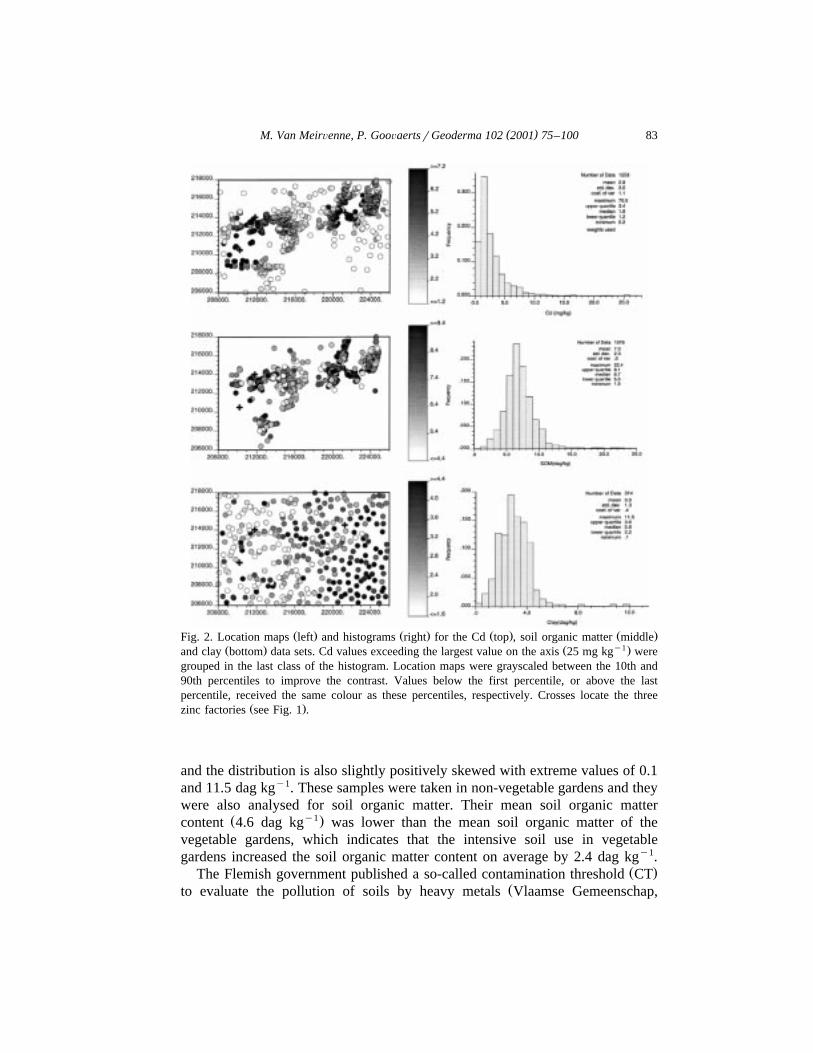
( )M. Van MeirÕenne, P. GooÕaertsrGeoderma 102 2001 75–100 83
Ž . Ž . Ž . Ž .Fig. 2. Location maps left and histograms right for the Cd top , soil organic matter middleŽ . Ž y1.and clay bottom data sets. Cd values exceeding the largest value on the axis 25 mg kg were
grouped in the last class of the histogram. Location maps were grayscaled between the 10th and90th percentiles to improve the contrast. Values below the first percentile, or above the lastpercentile, received the same colour as these percentiles, respectively. Crosses locate the three
Ž .zinc factories see Fig. 1 .
and the distribution is also slightly positively skewed with extreme values of 0.1and 11.5 dag kgy1. These samples were taken in non-vegetable gardens and theywere also analysed for soil organic matter. Their mean soil organic matter
Ž y1.content 4.6 dag kg was lower than the mean soil organic matter of thevegetable gardens, which indicates that the intensive soil use in vegetablegardens increased the soil organic matter content on average by 2.4 dag kgy1.
Ž .The Flemish government published a so-called contamination threshold CTŽto evaluate the pollution of soils by heavy metals Vlaamse Gemeenschap,

( )M. Van MeirÕenne, P. GooÕaertsrGeoderma 102 2001 75–10084
.1996 . It is used to decide whether a soil is suitable for a particular land useŽ . Ž .concentration-CT or whether sanitation measures like cleaning up are
Ž .required concentration)CT . It is computed according to:
aqbCqcOCT C,O sN 10,2 15Ž . Ž . Ž .ž /aq10bq2c
Ž y1. Ž y1.whereC is the clay content dag kg ,O the soil organic matter dag kg ,Ž . Ž .CT C,O is the CT, andN 10,2 , a, b and c are parameters depending on the
type of heavy metal and the type of land use. For Cd,as0.4, bs0.03,Ž . Ž .cs0.05 and for agricultural land use including vegetable gardens ,N 10,2 s2
mg kgy1.
3. Exceedence of the location-specific sanitation threshold
3.1. Cadmium
3.1.1. Soft indicator codingThe nine deciles of the declustered sample distribution of Cd were used as
Ž .thresholdsz . Using Eq. 5 , all observations were soft indicator coded with ak
CV of 7.8%.
3.1.2. Spatial trend— local meansTwo processes were considered to be responsible for the clearly observable
Ž .spatial trend in the Cd data Fig. 2 : the dominant winds and the distance to theŽ .sources the three factories causing a dilution effect.
Ž .A wind rose from a climatic station Kleine Brogel near the study area isgiven in Fig. 3. The dominant winds blow to the north to east directions. This
ŽFig. 3. Wind rose of annual frequencies of wind blowing to a particular direction longest.line—NNE—corresponds to 12.5% .

( )M. Van MeirÕenne, P. GooÕaertsrGeoderma 102 2001 75–100 85
Žwind rose was split into four directional classes 4.4% of the days of the year it.is windless defined as:
v Ž . Ž .High frequency 54.9% : angle interval 3488 to 1018 Es08v Ž .Medium frequency 24.4% : angle interval 1468 to 2368,v Ž .Relatively low frequency 11.1% : angle interval 2368 to 3488, andv Ž .Low frequency 5.2% : angle interval 1018 to 1468.
Nine distance classes were considered around each factory: 0–499, 500–999,1000–1499, 1500–1999, 2000–2999, 3000–3999, 4000–4999, 5000–5999 andG6000 m. Assuming that the major source of contamination for any sampled
Ž .Fig. 4. Trend surfaces corresponding to 1—the local mean indicator of the probability to exceedŽ y1 . Ž y1 . Ž y1 .the 20% 1.8 mg kg , top , the 50% 3.1 mg kg , middle and the 80% 5.4 mg kg , bottom
percentile of the Cd distribution.

( )M. Van MeirÕenne, P. GooÕaertsrGeoderma 102 2001 75–10086
Ž .locationx is the closest of the three factories, each indicator datai x ; z wasa a k
assigned to one directional and one distance class. For each threshold valuez ,k
the indicators were averaged within each of these 36 classes resulting in a9=4=9 look-up table of local means describing the spatial trend of Cdconcentrations. To avoid abrupt changes across class boundaries, these local
Žmeans were smoothed by interpolation using ordinary kriging with a linear. Žvariogram model . Fig. 4 shows the resulting trend surfaces plotted as 1y
Ž ..i x; z for the 2nd, 5th and 8th decile valuez . As the threshold valuek k
increases, the spatial continuity of the local means decreases dramatically due tothe concentration of higher Cd values in the vicinity of the factories and alongthe most frequent wind directions.
3.1.3. IndicatorÕariograms of residualsŽ .For every z the local mean was subtracted from the indicatorsi x ; zk a k
Ž .yielding nine sets of residualsr x ; z . The omnidirectional variograms ofa kŽ Ž ..these residuals were calculated Eq. 11 and fitted by a combination of a
Ž . Ž .nugget effect and a spherical first four or an exponential last five modelŽ . Ž .McBratney and Webster, 1986 Table 1 and Fig. 5 . The gradual increase ofthe ratio of the nugget effect vs. the sill from 43% to 83% and the correspondingdecrease in the range reflect a gradual spatial destructuring as the Cd valuesincrease.
3.1.4. Simple indicator kriging withÕarying local means and ccdfsCcdf values of Cd were estimated by simple indicator kriging with varying
Ž Ž . Ž ..local means Eqs. 9 and 10 . The latter were provided by the trend surfacesŽat the nodes of a 200 m=200 m grid. A search radius of 1200 m correspond-
.ing to the largest range of the fitted variograms, see Table 1 was used and aminimum of four neighbouring observations was required before an interpola-
Table 1Ž .Parameters of the nine fitted indicator variograms of the Cd residuals Fig. 5
y1 aŽ . Ž .z mg kg Nugget Model Sill Range mk
1.2 0.042 Sph 0.055 11651.8 0.064 Sph 0.074 12202.2 0.081 Sph 0.071 10502.6 0.089 Sph 0.069 9003.1 0.077 Exp 0.077 8253.6 0.081 Exp 0.057 9154.3 0.074 Exp 0.027 7005.4 0.052 Exp 0.011 1707.3 0.025 Exp 0.009 85
aSph: spherical, Exp: exponential.

()
M.
Va
nM
eirÕe
nn
e,P
.G
ooÕa
ertsr
Ge
od
erm
a1
02
20
01
75
–1
00
87
Ž .Fig. 5. Indicator variograms of Cd residualsr x ; z for the nine thresholdsz .a k k

( )M. Van MeirÕenne, P. GooÕaertsrGeoderma 102 2001 75–10088
tion was accepted. The number of neighbours was limited to the closest 25 ifmore were available within the search radius. Due to the uneven spatialcoverage of the Cd observations this condition was fulfilled at only 3164 out of5400 grid nodes. At each of these locations, the interpolated probabilities were
Ž Ž ..used to construct the ccdfs. The means of the ccdfs Eq. 13 are mapped inFig. 6. As expected, the largest Cd concentrations were found near the factorieswith extensions along the major wind directions.
3.2. Soil organic matter and clay
Due to the absence of a dominant spatial trend for soil organic matter andŽ .clay see Fig. 2 , the ccdfs of both variables were obtained by ordinary indicator
Ž Ž .. Žkriging Eq. 7 . Again, nine thresholds corresponding to the nine deciles 0.1. Ž .to 0.9 of the sample distributions Fig. 2 , were used for the soft indicatorŽ Ž ..coding Eq. 5 using the reported repeatabilities. Isotropic indicator variograms
Ž .not shown were computed and modelled for both variables and each of thenine thresholds. Because of the more restricted spatial coverage of soil organicmatter compared to Cd, only 2925 grid nodes could be interpolated. At thoselocations, the ccdfs of soil organic matter and clay were constructed using the
Ž .same options to correct order relation problems and to extrapolate at the tailsas for Cd.
3.3. Cross-Õalidation of spatial predictions of Cd, soil organic matter and clay
Before making any decision on the basis of uncertainty models it is critical toevaluate how well the ccdfs capture the uncertainty about the unknown values.
Ž y1. ŽFig. 6. Map of Cd mg kg E-type estimates circles locate factories; values larger than 10 werecoloured as 10, largest values10.9 mg kgy1; white areas could not be interpolated under the
.imposed conditions .
( )M. Van MeirÕenne, P. GooÕaertsrGeoderma 102 2001 75–100 89
As for spatial interpolation, a classical approach is to compare geostatisticalpredictions with observations that have been temporarily removed one at a timeŽ .leave-one-out or cross-validation approach . The major difficulty resides in theselection of performance criteria for ccdfs modeling.
Ž .At any test locationx , a series of symmetricp-probability intervals PI can0Ž .be constructed by identifying the lower and upper bounds to the 1yp r2 and
Ž . Ž <Ž ..1qp r2 quantiles of the ccdfF x ; z n , respectively. For example, the0w y1Ž <Ž ..0.5yPI will be bounded by the lower and upper quartilesF x ; 0.25 n ,0
y1Ž <Ž ..xF x ; 0.75 n . A correct modelling of local uncertainty would entail that0
there is a 0.5 probability that the actualz-value atx falls into that interval or,0
equivalently, that over the study area 50% of the 0.5yPI include the true value.ŽIf a set of ccdfs have been derived independently from z measurements e.g.
.using cross-validation or jackknife atN data locationsx , the fraction of truej
values falling into the symmetricpyPI is readily computed as:N1
j p s j x ; p ; pg 0, 1 16Ž . Ž . Ž .Ý jN js1
with:
j x ; pŽ .j
y1 y1< <1 if z x g F x ; 1yp r2 n ,F x ; 1qp r2 nŽ . Ž . Ž . Ž . Ž .Ž . Ž .j j js ½0 otherwise17Ž .
Ž .To account for measurement errors,j x ; p is here computed as:j
j x ; pŽ .j
y1 < y1 <sProb F x ; 1yp r2 n -z x FF x ; 1qp r2 n .Ž . Ž . Ž . Ž . Ž .Ž . Ž .½ 5j j j
18Ž .Ž . Ž .The closeness of the estimated experimental and expected theoretical frac-
Ž .tions can be assessed using the goodness statisticsG Deutsch, 1997 defined as:
1Gs1y 3a p y2 j p yp d p 19Ž . Ž . Ž .H
0
Ž .where a p is an indicator function defined as:
1 if j p GpŽ .a p s 20Ž . Ž .½0 otherwise.
Ž . Ž .Twice more importance is given to deviations whenj p -p inaccurate case< Ž . <since then 3a p –2 s2. In the case where the fraction of true values falling

( )M. Van MeirÕenne, P. GooÕaertsrGeoderma 102 2001 75–10090
into the p-probability interval is larger than expected, i.e. the accurate case, thisweight becomes 1. In other words, one penalizes the situation where the fractionof true values within the PI is smaller than expected. The ideal situation is whenthe experimental fractions match the theoretical ones, that isGs1. Thegoodness statistics is completed by the so-calledAaccuracy plotB which is a plotof the experimental vs. expected fractions.
A cross-validation approach has been used to derive ccdfs of Cd, soil organicmatter and clay content at, respectively,Ns1553, 1378 and 314 data locationsof Fig. 2. Probability intervals have been computed for increasing probabilitypand the proportions of true values falling into these PIs were computed
Ž .according to Eq. 16 . Fig. 7 shows that for Cd the dots plot on the 458 line,which indicates that the theoretical fractions are correctly predicted by our
Ž .uncertainty modelsG close to 1 . Results are not as good for the two other
Ž .Fig. 7. Plots of the proportion of true values falling within probability intervals accuracy plot vs.the probabilityp. Ccdfs for Cd, organic matter and clay were derived using indicator kriging andcross-validation, while the ccdfs of the difference between Cd and the CT were obtainednumerically using the Latin hypercube sampling procedure described in Fig. 8.

( )M. Van MeirÕenne, P. GooÕaertsrGeoderma 102 2001 75–100 91
properties: the dots lying below the 458 line for p)0.5 means that theproportion of true values falling into largep-probability intervals is smaller thanexpected, which reflects a less accurate modeling of the tails of the ccdfs.Deviations between experimental and theoretical fractions are however smallsince the goodness statistics are all very close to 1.
3.4. Latin hypercube sampling
3.4.1. Sanitation thresholdAt each of the 2925 grid nodes, the ccdfs of soil organic matter and clay were
discretised into 100 equiprobable classes which were randomly sampled eachŽonce and independently for both variables the correlation coefficient between
the 314 clay and soil organic matter values of the Belgian Soil Survey was0.173, and their correlation should be even smaller on vegetable gardens due to
.the strong impact of gardening practice on soil organic matter . This yielded, foreach grid node, 10 000 pairs of soil organic matter and clay values which were
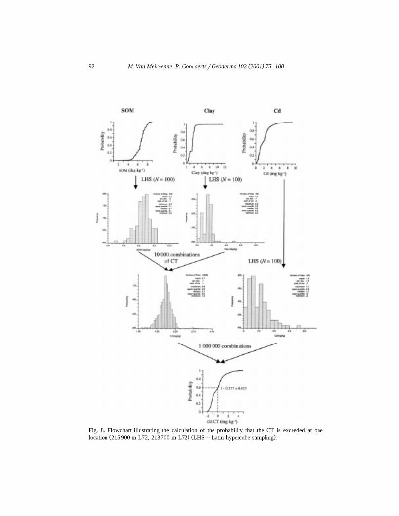
Ž .combined into Eq. 15 to generate a set of 10 000 CT values. Fig. 8 illustratesthis procedure for one location. Fig. 9 shows a map of the mean of the local
Ž Ž ..distributions Eq. 13 of the 10 000 CT values. The spatial variability of soilorganic matter and clay, together with the analytical uncertainty, yielded CTvalues ranging between 1.60 and 2.51 mg kgy1, with an average of 2.08 mgkgy1.
3.4.2. Probability to exceed the CTAt the same 2925 grid nodes, the ccdf of the Cd content was also sampled by
Ž .a Latin hypercube sampling Fig. 8 . The resulting set of 100 Cd values wascompared with the set of 10 000 CT values yielding a ccdf based on 1 000 000differences between Cd and CT. The underlying assumption here is the indepen-dence between CT and Cd values, the correlation of which could not be formallyassessed since there is no location where all variables are known. In presence ofa likely positive correlation between Cd and ST, an independent sampling oftheir probability distributions as performed in this paper would entail an
Ž .overestimation of the actual risk of exceeding the CT conservative scenario .Note that if the correlation can be estimated, procedures exist to sample jointlyprobability distributions so that the simulated values reproduce the experimental
Ž .correlation Heuvelink, 1998 . The probability of exceeding the threshold wasŽ .estimated by the proportion of these differences that are positive Fig. 8 and
these probabilities are mapped in Fig. 10. The probability of exceeding the CTvaried between 0 and 1 with a mean of 0.62. As expected, high probabilitieswere found around the factories, but due to the spatial variability of all threevariables involved, the spatial pattern of the probability to exceed the CT is
Ž .much more complex than that of Cd compare to Fig. 6 .
( )M. Van MeirÕenne, P. GooÕaertsrGeoderma 102 2001 75–10092
Fig. 8. Flowchart illustrating the calculation of the probability that the CT is exceeded at oneŽ . Ž .location 215900 m L72, 213700 m L72 LHSsLatin hypercube sampling .

( )M. Van MeirÕenne, P. GooÕaertsrGeoderma 102 2001 75–100 93
Ž y1.Fig. 9. Map of the mean of the local distribution of 10000 CT mg kg values obtained throughŽ .a Latin hypercube sampling of the ccdfs of soil organic matter and clay circles locate factories .
The goodness of the ccdfs of the difference between Cd and CT was assessedusing a cross-validation approach similar to the one described above. A diffi-culty was that such a cross-validation requires the knowledge of all three soilproperties at the same locations, which is not the case here. Such a limitationwas overcome by using only those 1364 locations where both Cd and organicmatter content have been measured and by interpolating clay content at theselocations using ordinary kriging. The later estimates have been considered astrue values in the cross-validation approach. At each location, the three ccdfshave been sampled using the procedure described in Fig. 8 to yield a numeri-
Fig. 10. Probability map to exceed the local CT.

( )M. Van MeirÕenne, P. GooÕaertsrGeoderma 102 2001 75–10094
cally cross-validated ccdf of the difference between Cd and CT. The accuracyŽ .plot of Fig. 7 right bottom graph shows that these models predict very well the
proportions of true values that fall within probability intervals of increasing sizeŽ .Gs0.98 .
3.5. AdÕantages of the proposed procedure
The following are the advantages of our procedure.Ž .1 Any probability thresholdp can be considered in decision-making. Forc
example, if we would consider the 80% probability of exceeding CT as a criticalprobability level p , thenx would be classified as contaminated if:c 0
<Prob Z x )z n Gp . 21� 4Ž . Ž . Ž .0 c c
In our case study, ifp s0.80 this would result in a classification of 27.3% ofcŽ .the interpolated area covering 3192 ha as unsafe to be used as vegetable
gardens, i.e. where Cd exceeds the CT. To avoid the difficult selection of aŽ .probability threshold for criterion 21 , an alternative consists of classifying as
hazardous all locations where the CT is exceeded in expected value:
x is hazardous ifE Cd x )E CT x or if E Cd x yCT x )0.Ž . Ž . Ž . Ž .0 0 0 0 0
22Ž .
The expected value of the difference between the Cd and CT values wasnumerically approximated by the arithmetic average of the 1 000 000 differencesgenerated by the Latin hypercube sampling of the ccdfs. According to this
Ž .criterion, the largest part of the interpolated area 72.7% or 8492 ha wasŽ .classified as hazardous Fig. 11 .
Fig. 11. Classification of locations as hazardous or safe on the basis that the Cd sanitationŽ Ž ..threshold is exceeded in expected value Eq. 22 .

( )M. Van MeirÕenne, P. GooÕaertsrGeoderma 102 2001 75–100 95
Ž . Ž .2 Because the decision rule 22 involves expected values, there is actuallyŽ .a risk that the locationx is wrongly declared hazardous false positive or safe0
Ž . Ž .false negative . These can be computed directly from our results Fig. 10Ž .Goovaerts, 1997; Myers, 1997 .
Ž .3 Using the concept of cost functions, an evaluation of the economic costsŽ .involved can be performed Goovaerts et al., 1997 .
An additional, but less often explored, advantage of our procedure is theability to optimise the location of additional samples.
4. Location of additional samples
When we are very uncertain about the actual pollutant concentrations and theresulting risk of misclassification, it might be more advantageous to collectadditional information before a final classification into safe or contaminated
Ž .areas is being conducted Van Groenigen, 1999 . Consider that additionalresources are available, allowing the collection ofS additional samples and themeasurement of Cd concentration, organic matter and clay contents. To increasethe cost-effectiveness of the new sampling phase, it is important to account forthe information already collected and processed.
4.1. Reduction of the uncertainty about Cd concentration
A first objective may be the reduction of the uncertainty about the Cdconcentration, which is achieved by sampling theS locations with the largestccdf variance for Cd:
q` 22 ) <x is sampled ifs x s zyz x f x,z n dz is large 23� 4Ž . Ž . Ž . Ž .Ž .H E0
Ž <Ž .. Ž . )Ž .where f x; z n is the local probability density function ofZ x , and z x isEŽ . Ž Ž .. Ž .the E-type estimate ofZ x Eq. 13 . Fig. 12 left column, top map shows the
map of the ccdf variance for Cd, and the 200 locations with the largest varianceŽ . Žleft middle map . Because of heteroscedasticity i.e. relation between local
.mean and local variance , the selected locations are all in the vicinity of thethree factories. Moreover, they are strongly clustered, hence additional con-straints must be imposed to avoid the collection of redundant information ofthese spatially autocorrelated variables. Now assume thatSs50 and that we
Žaccept 500 m as a maximal autocorrelation length as a compromise between the.different ranges of the indicator variograms, see Table 1 . With this additional
information we made a selection by starting from the location with the largestvariance and remove all other location within 500 m. Next, the location with thesecond largest variance was selected and again all locations within 500 m were

( )M. Van MeirÕenne, P. GooÕaertsrGeoderma 102 2001 75–10096
ŽŽ y1.2. Ž . Ž Ž ..Fig. 12. Top left: map of ccdf variance for Cd mg kg ; top right: map of CVx Eq. 24 ;location of 200 locations candidate for additional sampling because of the large ccdf variance for
Ž . Ž . Ž .Cd left middle or large CVx right middle ; bottom graphs show 50 locations with large ccdfŽ . Ž . Ž .variance for Cd left or large CVx right that are at least 500 m apart to increase the efficiency
Žof the sampling design circles in top maps and crosses in middle and bottom graphs locate.factories .
removed. This procedure continued until 50 locations were obtained with thelargest variance and that are at least 500 m apart, which increases the efficiency
Ž .of the sampling. Fig. 12 left bottom map shows the result.
4.2. Reduction of the remediation error
In many situations, the primary concern is to assess the intensity and realextent of pollution concentrations exceeding a regulatory threshold. In otherwords, it is the remediation decision that matters, not the accuracy of the
Ž .prediction itself Rautman, 1997 . The objective would then be to minimise theuncertainty about whether the critical thresholdz is exceeded.c

( )M. Van MeirÕenne, P. GooÕaertsrGeoderma 102 2001 75–100 97
Ž .Chien 1998 proposed assessing the uncertainty at the unsampled locationxŽ . 2Ž . 2Ž .by the productv x s x , wheres x is the conditional variance, a measure of
Ž . Ž .local uncertainty as defined in Eq. 23 andv x measures how close theprobability of exceeding the critical threshold atx is to the probability threshold
Ž .p specified by the decision-maker. Garcia and Froidevaux 1997 used as ac
measure of uncertainty the absolute difference between the probability ofexceeding the critical thresholdz and the closest of the two low and high riskc
probability thresholds 0.2 and 0.8; they considered that the uncertainty isnegligible at locations where the probability of contamination is either highŽ . Ž .)0.8 or low -0.2 . None of these methods take into account the fact thatthe predictions of the site-specific physical thresholdz may be uncertain, as inc
our case study. Therefore, we propose to use as a sampling criterion the ratio ofthe standard deviation to the absolute value of the mean of the local cumulative
Ž Ž .. Ž Ž ..distribution of the differenceD x between the pollutant concentrationZ xŽ Ž ..and the thresholdZ x :CT
Var D x( Ž .x is sampled if CVx s is large 24Ž . Ž .
< <E D xŽ .
Ž <Ž ..The expected value and the variance ofF x;d n were approximated byD
the arithmetical average and variance of the 1 000 000 differences between Cdand CT generated by the Latin hypercube sampling of the ccdfs. This type of
Ž .coefficient of variation CV is large if the denominator is small, that is if thesimulated pollutant concentrations and threshold values are close and so theuncertainty about the exceedence of that threshold becomes large. For the sameaverage difference, the CV will be larger if the variance of the distribution ofdifferences is large.
Ž . Ž . Ž .Fig. 12 right column shows the map of CVx top , and the 200 locationswith the largest values are displayed below it. Unlike the previous criterion,additional samples are no longer collected in the vicinity of factories, which iscertainly contaminated, but the focus is on the borderline between the zones that
Ž .could be classified as safe or hazardous compare to Fig. 11 . Indeed, it is inthese areas that the risk for misclassification is the largest. Although theclustering is less pronounced than for the first criterion, the efficiency of thesampling can be increased by imposing a constraint of minimum distancebetween two samples; for example a minimum distance of 500 m leads to the
Ž .selection of the 50 locations displayed at the bottom of Fig. 12 right graph ,using the same selection procedure as described before. This selection could be
Ž .optimised further using simulated annealing Van Groenigen and Stein, 1998 ;Ž .for example, the two constraints of maximisation of CVx and maximisation of
the distance between samples could be included into a single objective functionŽinstead of imposing a constraint of minimum distance a posteriori two-step
.approach .

( )M. Van MeirÕenne, P. GooÕaertsrGeoderma 102 2001 75–10098
5. Conclusions
The environmental database of our study consisted of three soil variables: Cd,soil organic matter and clay. These data had several characteristics complicatingtheir combined spatial evaluation:
v Soil organic matter was collocated with Cd, but clay was not.v Cd and soil organic matters were strongly spatially clustered, but only for Cd
high-valued areas were preferentially sampled. A declustering procedure wasused to obtain a Cd distribution that is representative of the study area.
v ŽThe distributions of these variables were moderately soil organic matter and. Ž .clay to strongly Cd positively skewed.
v Cd displayed a strong spatial trend due to the preferential winds and theŽ .distance to its sources three factories .
v Ž .The analytical repeatability varied between 2.2% for soil organic matter toŽ .7.8% for Cd .
The aim of this paper was to present a non-parametric methodology toincorporate two common sources of uncertainty, spatial interpolation and analyt-ical error, into the prediction of the probability of exceeding a location-specific
Ž .threshold. The combination of non-stationary in the case of Cd indicatorkriging and Latin hypercube sampling yielded local ccdfs of the differencebetween the heavy metal concentration and the CT. Knowledge of such ccdfsallowed the mapping of the probability of exceeding that threshold, i.e. in our
Ž .case study this amounted to 27.3% of the interpolated area 3190 ha where theprobability to exceed the CT is 80% or higher. Cross-validation results indicatedthat most ccdf models are accurate in that the fraction of true values falling intoa p-probability interval is usually larger than expected.
The design of a sampling scheme that minimises the averaged krigingvariance over the study area typically leads to take additional samples insparsely sampled areas. Although it is important to account for first-phasesampling density in the elaboration of the second-phase design, data values mustalso be accounted for, in particular in the presence of heteroscedasticity. In thiscase, the uncertainty may be larger in an area that is densely sampled but whichdisplays higher variabilities than in a sparsely sampled area that is homoge-neous. Whereas minimisation of uncertainty about Cd concentration entails the
Žsampling of high-valued areas around factories, the proposed approach i.e.minimisation of theAcoefficient of variationB of the ccdf of differences between
.Cd concentration and the CT leads to the sampling of borderlines between areasclassified as hazardous or safe. Because the ccdfs are data-dependent, onecannot investigate a priori the impact of the sampling strategy on the localuncertainty, as is possible when the kriging variance is used as a measure of
Ž .uncertainty Burgess et al., 1981 . Thus, additional constraints, such as mini-

( )M. Van MeirÕenne, P. GooÕaertsrGeoderma 102 2001 75–100 99
mum distance between samples, need to be imposed to avoid clustering ofsamples and the consequent loss of efficiency of the sampling design.
Acknowledgements
Ž . Ž . ŽJ. Hendrickx community of Balen , G. Ide LISEC , W. Mennen community. Ž .of Lommel , A. Stein Landbouwuniversiteit Wageningen , J. Vangronsveld
Ž . ŽLimburgs Universitair Centrum , and D. Wildemeersch Vlaamse Gemeen-.schap are kindly thanked for providing the Cd and soil organic matter data.
This research was conducted during a leave of the first author at The Universityof Michigan for which he gratefully acknowledges the financial support of the
Ž .Flemish Fund for Scientific Research FWO . The authors also wish to expresstheir gratitude to the reviewers for their constructive remarks.
References
Burgess, T.M., Webster, R., McBratney, A.B., 1981. Optimal interpolation and isarithmicmapping of soil properties: IV. Sampling strategy. Journal of Soil Science 31, 315–331.
Burrough, P.A., McDonnell, R.A., 1998. Principles of Geographical Information Systems. OxfordUniv. Press, Oxford, 333 pp.
Chaney, R.L., 1990. Public health and sludge utilization, part II. BioCycle 31, 68–73.Chien, Y.-J., 1998. A Geostatistical Approach to Sampling Design for Contaminated Site
Characterization. Master Thesis, Stanford University, Stanford, CA.Deutsch, C.V., 1997. Direct assessment of local accuracy and precision. In: Baafi, E.Y., Schofield,
Ž .N.A. Eds. , Geostatistics Wollongong ’96. Kluwer Academic Publishing, Dordrecht, pp.115–125.
Deutsch, C.V., Journel, A.G., 1998. GSLIB Geostatistical Software Library and User’s Guide.Oxford Univ. Press, New York.
Englund, E.J., Heravi, N., 1994. Phased sampling for soil remediation. Environmental andEcological Statistics 1, 247–263.
Garcia, M., Froidevaux, R., 1997. Application of geostatistics to 3-D modelling of contaminatedŽ .sites: a case-study. In: Soares, A. Ed. , geoENV I—Geostatistics for Environmental Applica-
tions. Kluwer Academic Publishing, Dordrecht, pp. 309–325.Goovaerts, P. et al., 1994. Comparative performance of indicator algorithms for modeling
conditional probability distribution functions. Mathematical Geology 26, 389–411.Goovaerts, P., 1997. Geostatistics for Natural Resources Evaluation. Oxford Univ. Press, New
York, 483 pp.Goovaerts, P., 1999. Geostatistics in soil science: state-of-the-art and perspectives. Geoderma 89,
1–45.Goovaerts, P., Journel, A.G., 1995. Integrating soil map information in modelling the spatial
variation of continuous soil properties. European Journal of Soil Science 46, 397–414.Goovaerts, P., Webster, R., Dubois, J.-P., 1997. Assessing the risk of soil contamination in the
Swiss Jura using indicator geostatistics. Environmental and Ecological Statistics 4, 31–48.Heuvelink, G.B.M., 1998. Error Propagation in Environmental Modeling with GIS. Taylor,
Francis, London, 127 pp.

( )M. Van MeirÕenne, P. GooÕaertsrGeoderma 102 2001 75–100100
Journel, A.G., 1983. Non-parametric estimation of spatial distributions. Mathematical Geology 15,445–468.
Journel, A.G., 1986. Constrained interpolation and qualitative information. Mathematical Geology18, 269–286.
Journel, A.G., Huijbregts, A.G., 1978. Mining Geostatistics. Academic Press, New York, 600 pp.Juang, K.-W., Lee, D.-Y., 1998. A comparison of three kriging methods using auxiliary variables
in heavy-metal contaminated soils. Journal of Environmental Quality 27, 355–363.Luxmoore, R.J., King, A.W., Tharp, L., 1991. Approaches to scaling up physiologically based
soil-plant models in space and time. Tree Physiology 9, 281–292.McBratney, A.B., Webster, R., 1986. Choosing functions for semi-variograms of soil properties
and fitting them to sampling estimates. Journal of Soil Science 37, 617–639.McKay, M.D., Beckman, R.J., Conover, W.J., 1979. A comparison of three methods for selecting
values of input variables in the analysis of output from a computer code. Technometrics 21,239–245.
Myers, J.C., 1997. Geostatistical Error Management. Van Nostrand-Reinhold, New York, 571 pp.Ž .OFEFP Office federal de l’environnement, des forets et du paysage , 1993. Reseau national´ ´ ˆ ´
d’observation des sols, periode d’observation 1985–1991. Cahier de l’environnement no. 200,´Berne, Swiss.
Pebesma, E.J., Heuvelink, G.B.M., 1999. Latin hypercube sampling of Gaussian random fields.Ž .Technometrics accepted for publication .
Rautman, C.A., 1997. Geostatistics and cost-effective environmental remediation. In: Baafi, E.Y.,Ž .Schofield, N.A. Eds. , Geostatistics Wollongong ’96. Kluwer Academic Publishing, Dor-
drecht, pp. 941–950.Tiktak, A., Leijnse, A., Vissenberg, H., 1999. Uncertainty in a regional-scale assessment of
cadmium accumulation in the Netherlands. Journal of Environmental Quality 28, 461–470.Van Groenigen, J.W., 1999. Constrained optimisation of spatial sampling—a geostatistical
approach. PhD Thesis, Wageningen Agricultural University and ITC Enschede, 148 pp.Van Groenigen, J.W., Stein, A., 1998. Constrained optimization of spatial sampling using
continuous simulated annealing. Journal of Environmental Quality 27, 1078–1086.Van Meirvenne, M., 1991. Characterization of soil spatial variation using geostatistics. PhD thesis,
University of Gent.Vlaamse Gemeenschap, 1996. Besluit van de Vlaamse regering houdende vaststelling van het
Vlaams reglement betreffende de bodemsanering. Belgisch Staatsblad dd. 27.03.1996, pp.7018–7058.
Webster, R., Burgess, T.M., 1984. Sampling and bulking strategies for estimating soil propertiesof small regions. Journal of Soil Science 35, 127–140.


