Evaluating the use of recycled coal combustion products in constructed wetlands: an ecologic-economic modeling approach

Ecological Modelling 150 (2002) 117–140

Evaluating the use of recycled coal combustion products inconstructed wetlands: an ecologic-economic modeling

approach

Changwoo Ahn, William J. Mitsch *En�ironmental Science Graduate Program and School of Natural Resources, The Ohio State Uni�ersity, 2021 Coffey Road,

Columbus, OH 43210-1085, USA

Received 23 January 2001; received in revised form 22 October 2001; accepted 31 October 2001

Abstract

A simulation model was developed to couple the biogeochemistry of phosphorus removal with the potentiallyeconomical and environmentally beneficial use of a coal combustion waste product as a liner in constructed wetlands.The model includes hydrology, macrophyte and phosphorus submodels coupled to an economic accountingsubmodel. Data from two constructed wetlands in central Ohio, USA, the Olentangy River Wetland and the LickingCounty Wetland (LCW), fed by low and high nutrient loads, respectively, were used to calibrate and validate theecologic portion of the model. The model was used to provide parameters in design of a pilot-scale treatment wetlandunder construction to test flue-gas-desulfurization (FGD) by-products as a liner material. Subsequent modelsimulations of the LCW with a liner for prediction of phosphorus retention efficiency showed enhanced phosphorusretention (�10% by mass) and economic benefits if the wetland were lined with the FGD by-product relative to clay.Total cost saving (liner cost saving plus phosphorus treatment saving) of recycling FGD by-products predicted by themodel is closely related to both wetland size and phosphorus loading. Total savings of using FGD by-products as aliner over clay in the LCW (6.4 ha) was calculated at approximately US $ 23 000 years−1 for 30 years at 8% interestrate assumed. © 2002 Elsevier Science B.V. All rights reserved.

Keywords: Coal combustion product; Flue-gas-desulfurization (FGD); Liner; Unit cost of phosphorus removal; Constructedwetland; Olentangy River Wetland Research Park

www.elsevier.com/locate/ecolmodel

1. Introduction

Nearly 90% of the electricity produced in Ohio,USA, is generated from coal burning and the state

generates about 12% (11.6 million tons) of all coalcombustion products (CCPs) in the United States(American Coal Ash Association Survey, 1997).These products, generated in large quantities,have traditionally been treated as wastes and dis-posed of in expensive, non-productive landfills.However, the disposal of this enormous volume ofwaste becomes increasingly difficult as landfill

* Corresponding author. Tel.: +1-614-292-9774; fax: +1-614-292-9773.

E-mail address: [email protected] (W.J. Mitsch).

0304-3800/02/$ - see front matter © 2002 Elsevier Science B.V. All rights reserved.

PII: S0 304 -3800 (01 )00477 -X

mailto:[email protected]

C. Ahn, W.J. Mitsch / Ecological Modelling 150 (2002) 117–140118

costs increase and landfill spaces decrease. Flue-gas-desulfurization (FGD) by-product, one ofthe CCPs, is the result of lime scrubbing of sul-fur oxides from flue gases of coal-fired electricalgenerating stations to reduce acid deposition.More than 7.5 million tons of FGD by-productare produced annually in Ohio, making it thelargest single-produced material in the state(Wolfe et al., 2000).

Efforts have been made to reuse FGD wastesin such beneficial ways as in highway and civilengineering applications, as waste-storage pondliners, and as an agricultural liming substitute inlivestock feeding pads (Wolfe et al., 2000). Onepotential use of FGD by-product is as a linerfor the construction of treatment wetlands. Ahnet al. (2001) tested FGD by-products as liners inconstructed wetlands through 1-m2 mesocosmexperiments over two years. Their resultsshowed not only the possibility of the materialas an alternative liner to commonly used com-mercial clay or bentonite, but also the potentialof additional phosphorus retention in the treat-ment wetlands as a result of the FGD materialitself.

There are three potential benefits of recyclingFGD by-products as a liner in constructed wet-lands to treat nutrients over natural or commer-cial clay materials. These benefits are:1. Lower costs for obtaining the recycled FGD

by-product for liners as the material is basi-cally free except for handling and haulingcosts.

2. Reduction in volume of a waste product thatis otherwise disposed of in landfills.

3. Enhanced phosphorus retention due to thechemical characteristics of the FGD liner ma-terial (Ahn et al., 2001).

Dynamic models of phosphorus retention inwetlands have been studied extensively (Kadlecand Hammer, 1988; Mitsch and Reeder, 1991;Kadlec, 1997; Richardson et al., 1997; Wang andMitsch, 2000). Some studies have also attemptedto interlink ecology model and economic analysis(Baker et al., 1991; Breaux et al., 1995; Grant andThompson, 1997; Robles-Diaz-de-Leon andNava-Tudela, 1998; Cardoch et al., 2000). Fewstudies, however, have been conducted to connect

ecological functions of constructed wetlands (e.g.phosphorus retention) with their economic conse-quences through a combined ecologic-economicmodeling approach.

The goal of our study was to develop a dy-namic model which simulates phosphorus reten-tion incorporated with economic benefits ofrecycling FGD waste as a liner in constructedwetlands. This model allows an a priori costsaving calculation of recycling FGD by-productas liners relative to using clay material.

2. Site description

2.1. Olentangy Ri�er wetland (ORW)

Two 1-ha experimental wetland basins of theOlentangy River Wetland Research Park (OR-WRP) in Columbus, Ohio were constructed onalluvial, old-field soils adjacent to the third-or-der Olentangy River in 1994 (Mitsch et al.,1998). The wetlands are fed by the OlentangyRiver water. Nairn and Mitsch (2000) andSpieles and Mitsch (2000) described phosphorusand nitrogen retention in these experimentalbasins in detail.

2.2. A pilot-scale FGD-lined wetland system atthe ORWRP

A medium-scale FGD-lined wetland study iscurrently underway at the ORWRP. This is alarger-scale effort than the mesocosm studies(Ahn et al., 2001) to further investigate the ef-fects of FGD by-product recycled as liners intreatment wetlands. We expect this pilot-scalewetland study, being conducted over the nexttwo years (2001–2002), to provide essential in-formation before going to full-scale applicationof FGD by-products in building wetlands.

Four separate pilot wetland basins were con-structed (�3 m×7.8 m×1.5 m). All basinswere placed in parallel. A 0.15-cm plastic linerand a geo-membrane such as those used inlandfill caps were fitted to the four basins andwelded appropriately so that the material cov-

C. Ahn, W.J. Mitsch / Ecological Modelling 150 (2002) 117–140 119

ered both the wetland basins and the berms inbetween the basins. A layer of gravel approxi-mately 0.2–0.3 m deep was then added to thecells to serve as the subsurface strata of thesebasins. FGD by-product was then applied totwo of the basins and the berms in between,and compacted by excavating machinery to 0.3m. Recompacted clay was applied to the othertwo basins in the same fashion. Approximately0.3-m site soil obtained during the excavationwas then added to all four basins as a mediumfor wetland vegetation to grow in. We used thedynamic model we developed in this study tosuggest design parameters for this pilot-scalewetland. Hydraulic loading rate (cm days−1)and inflow TP concentration were manipulatedin the model to achieve optimal conditions forphosphorus retention in the model simulations.

2.3. Licking County Wetland

Licking County Wetland (LCW), located nearKirkersville, Ohio, was constructed in 1995 forthe tertiary treatment of municipal wastewatereffluent from the Southwest Licking CommunityWater and Sewer District treatment plant(Mitsch and Metzker, 1996; Spieles and Mitsch,2000). The wetland site consists of two 3.2-habasins built on alluvial, previously farmed soilswhich discharge water into the South Fork ofthe Licking River, a second order stream. Sec-ondarily treated wastewater has fed both theWetland North (LCWN) and the Wetland South(LCWS) since the spring of 1995. WetlandSouth (LCWS), however, proved to be leakyand did not retain water in 1996. Subsequently,all wastewater was routed to LCWN for the du-ration of the study. This specific condition ofLCWS may provide a good case for testingFGD waste as a liner in the future as our pilot-scale wetland study on the material reveals moreinformation. The model was thus applied to theLCW to simulate its ecologic-economic dynam-ics when lined with either clay or FGD by-product. The simulations calculated the potentialcost savings of recycling FGD by-products as aliner as well as phosphorus retention efficiencyin the LCW.

3. Simulation methods

The goal of the ecologic-economic wetlandmodel was to enable prediction of phosphorusretention and estimation of cost saving of build-ing wetlands lined with recycled FGD waste.Hydraulic loading rates and total phosphorus(TP) inflow concentrations over a 2-year period(1996–1997) from ORW basin 1 (ORW 1) andLCWN were used as input for model calibrationand validation to investigate general perfor-mance of the model in phosphorus retention.All initial conditions for the model were ob-tained from ORW 1 through previous studies(e.g. Harter and Mitsch, 1999). Four submodelswere developed such as hydrology, macrophyte,phosphorus and economic submodels. Each sub-model was linked to the previous submodel(s)and calibrated. A set of nonlinear, ordinary dif-ferential equations was used to describe the sub-models. The model was integrated using thesoftware STELLA™ V, a high level visual-ori-ented programming and simulation language foruse on Apple Macintosh™ computers (Rich-mond and Peterson, 1997). Fourth-orderRunge–Kutta was used as the integrationmethod with a time step of 0.1 weeks. Simula-tions were designed to run over a 2-years period(from 1 January of year 1 to 31 December ofyear 2) in constructed surface-flow wetlands.Calibration was carried out by adjusting selectedparameters in the model to obtain a best-fit be-tween model estimations and field data fromORW 1 for TP retention. A stepwise method(Mitsch and Reeder, 1991; Wang and Mitsch,2000) was used in this process by first calibrat-ing the hydrology submodel, then macrophytesubmodel, phosphorus submodel, and finallyeconomic model. At each step, values ofparameters determined during the previous stepwere not allowed to change from previously cal-ibrated values.

Sensitivity analysis is usually performed dur-ing model simulations to find the most impor-tant parameters which determines the main statevariables of interest (Jørgensen, 1988). Wangand Mitsch (2000) verified that TP inflow con-centration and phosphorus sedimentation coeffi-


cient (sed k in our model) were the most sensitiveparameters explaining TP retention in a dynamicphosphorus model of created wetlands. Therefore,we carried out sensitivity analysis of TP inflowconcentration and the sedimentation coefficient(sed k) on corresponding changes of TP retention(%) in our model runs with the LCW. The selectedparameters were varied by �2 orders of magnitudefor TP inflow concentration and by �10 through80% for sed k. Sensitivity analysis was also con-ducted in the economic submodel to investigate theeffects of changing inflow phosphorus loading onpotential economic benefits of FGD-lined wet-lands. Total annualized cost saving estimates werebased on a 30-year lifetime and 8% interest ratefollowing current industry practices. The sensitivityof these assumptions was also investigated. As-sumptions were made in developing the ecologic-economic wetland model, including the following:1. Vegetation uptake of phosphorus is from sedi-

ments and not from the water column(Richardson, 1985);

2. Phosphorus sedimentation is influenced byplant biomass (Kadlec and Knight, 1996);

3. A slight toxic effect of FGD by-product onearly development of macrophyte is expected(Ahn and Mitsch, 2001);

4. Enhanced phosphorus retention occurs be-cause of the FGD material (Ahn et al., 2001)and the rate is similar over the first 2-yearperiod of wetland operation;

5. The growing season for the model is for mid-temperate regions and begins early April andends mid September;

6. Seepage from the wetland basin is assumedzero with any liner being applied; and

7. No matter which material, either FGD by-product or clay, is used as a liner it needs to behauled to the wetland site from a similardistance.

4. Model description and calibration

A conceptual model of the constructed wetlandwith economic system is shown in Fig. 1. Differen-tial equations used for the model are presented inTable 1 and state variables, forcing functions and

parameters are summarized in Table 2. The modelis described in detail below.

4.1. Hydrology submodel

The hydrology submodel has only one statevariable, water volume (V), which balances apumped inflow, seepage and a surface outflow fromthe wetland. The hydraulic inflow loading based onfield data collected over the 2-year period (1996–1997) at ORW 1 (Table 3) was used in modelcalibration. Surface outflows were predicted byregression with wetland volume data for bothORW 1 and LCWN. Seepage to groundwater wasincluded as a function of wetland area. Seepagecoefficient (SC) was calibrated based on field esti-mation of seepage. In simulations of a constructedwetland with any liner being applied, either clay orFGD by-product, seepage was set to zero in themodel.

4.2. Macrophyte submodel

The macrophyte submodel includes two statevariables: biomass and detritus. Macrophyte pro-duction included only aboveground biomass in thismodel. A solar efficiency of 2.5% (e.g. Wang andMitsch, 2000) was estimated and applied to simu-late net primary productivity of macrophytes in thesubmodel. An estimated 20% reduction in plantgrowth was applied as a toxicity effect with a FGDmaterial (Ahn and Mitsch, 2001) only during thefirst growing season (13–38th week) of the wetlandmodel simulated with a FGD liner. An 0.8%recovery per week was applied to simulate themitigation of toxicity effects over that time as thepotential toxicity in experiments by Ahn andMitsch (2001) was observed to lessen, and wasnegligible in the second year with full-grown plants.The toxicity factor was designed as a conditionalsentence with an on/off switch (Table 1). It was alsoassumed that the dominant vegetation in thissystem is Schoenoplectus tabernaemontani, the mostcommon species in the constructed wetlands ex-plored in this study (�90% of vegetation cover).

Net primary productivity (NPP) depends onsolar energy, length of growing season, and FGDtoxicity factor. Frost is a pulse function that occurs


on the 41st week of the year. It signifies the firstfrost of the season that dispatches the livingbiomass stand into detritus. One other variable,standing stock, is included in the macrophytesubmodel, and is connected to the phosphorussubmodel. Standing stock, the sum of biomass and

detritus held above the surface of the wetlandsubstrate, is assumed to influence water movementand so positively affects the phosphorus sedimenta-tion rate in the phosphorus submodel whether aliveor dead. A similar approach in modeling macro-phyte dynamics was used in Baker et al. (1991) and

Fig. 1. Conceptual model of ecological-economic system of a constructed wetland with recycled coal combustion wastes: (a) detailphosphorus processes in a constructed wetland including FGD liner; and (b) connection between a constructed wetland shown in(a) with economics and society.


Table 1Differential equations used in the ecologic-economic wetland model

Hydrology submodeldV/dt(t)=Inflow−Outflow−SeepageWhere

Wetland water volume (m3)VPumped inflow from the field (m3 week−1)InflowRegression, surface outflow (m3 week−1) ORW: (3.8×10−5×V2)+(2.8×V)OutflowLCWN: (2.1×10−4×V2)+(0.6×V)If (FGD factor=1) then (0) else (V/Depth SC), seepage to groundwaterSeepage(m3 week−1)

Depth V/Aw, average water depth (m)Wetland area (m2)AwSeepage coefficient (m week−1)SC[V/((Inflow+Outflow)/2)]/7, hydraulic retention time (days)Tr

Macrophyte submodelNPP flow–LossdBiomass/dt=Loss–DecaydDetritus/dt=

WhereMacrophyte biomass in the wetland (g)BiomassSolar×MAC se×GS×FGDtf/R×Aw, macrophyte productivity (g week−1)NPP flowBiomass×(0.0007+frost), amount of energy entering the detritus from biomassLoss(g week−1)

Detritus Detritus (g)Decay Detritus×Decay R×FT, amount of energy lost from the detritus (g week−1)

4000–2000×cos(2×�×(time)/52), amount of solar energy flowing into theSolarwetland (kcal m−2 week−1)

MAC se Macrophytes solar efficiencyGS Growing season for biomass

If (FGD factor=1) then (Tx) else (1), FGD toxicity factorFGDtfTx Temporal pattern of initial toxicity of FGD being applied

Energy per biomass ratio (kcal g−1)RPulse function that occurs on the week 41 out of 52 weeksFrostDetritus decay rate (week−1)Decay R1.06�(Wtemp-20), temperature function for decayFT

Wtemp 15–13×cos(2×�×(time)/52), water temperature (°C)Biomass+Detritus (g)Standing stock

Phosphorus submodelUptake−loss PdBiomass P/dt=

WhereAmount of phosphorus found in biomass (g)Biomass PNPP flow×UTe, amount of phosphorus entering the biomass from sedimentsUptake(g week−1)

Loss P Loss×Le, amount of phosphorus entering the detritus from biomass (g week−1)Uptake efficiencyUTeLoss efficiencyLe

dDetritus P/dt=Loss P−decomp PWhere

Amount of phosphorus found in detritus (g)Detritus PDecay×De, amount of phosphorus being added to the sediment from detritusDecomp Pthrough decomposition (g week−1)

De Decay efficiency


Table 1 (Continued)

dSediment P/dt=Decompo P+ST-UptakeWhere

Amount of phosphorus found in the sediment (g)Sediment PIf (standing stock�4×106) then (Water P×STC/depth) else ((standingSTstock×5×10−8+STC)/depth×Water P), amount of phosphorus enteringthe sediment from water (g week−1)

Sed k Phosphorus sedimentation velocity (m week−1)

dWater P/dt=Inload−Outload−ST-P seepage-FGDeffectWhereWater P Amount of phosphorus found in the water (g)

Inflow×Inconc, amount of phosphorus entering the water columnInload(g week−1)Water P×Outflow/V(g week−1)OutloadIf (FGD factor=1) then (0) else (seepage×(Inconc+Outconc)/2),P seepagephosphorus loss from water column through seepage (g week−1)

FGD effect If (FGD factor=1) then (Water P×FGD CaP) else (0), additionalphosphorus retention by FGD (g week−1)

Inconc Total phosphorus concentration of inflow from the field (g m−3)Outconc Water P/V, total phosphorus concentration of outflow (g m−3)

Ca–P precipitation efficiencyFGD CaPP removal conc (In conc−out conc)/In conc×100, percent removal of phosphorus based

on concentration (%)(Inload−outload)/Inload×100, Percent removal of phosphorus based onP removal loadload (%)

P removed with clay (Inload−outload), amount of phosphorus removed with clay liner(g week−1)

P removed with FGD (Inload−outload)×1.1, amount of phosphorus with FGD liner(g week−1), 10% additional P retention assumed (e.g. Ahn et al., 2001)

Economic accounting submodelLiner cost saving −PMT (Interest rate, NY, Liner saving, 0), annualized payment on the

capital cost of a constructed wetland with FGD wastes ($ year−1); PMTfunction returns a negative value, indicating that the payment is anexpense, so (−) is applied to the PMT to produce (+) value of thesaving from the recycling of FGD wastes as liners.196336×(Wt area)�(−0.511)×(Wt area), regression equation forCost for wetlandcalculating the cost of wetland construction from Mitsch and Gosselink(2000) ($)(P removed with FGD-P removed with clay)×Unit cost of PP treatment savingwetland×52×2, amount of money saved by the enhanced removal ofphosphorus due to FGD by-products ($ year−1)

Interest rate 0.08, annual interest assumed (8%)NY 30, lifetime of constructed wetland assumed (year)

Annualized cost saving+FGD treat saving ($ year−1)Total savingsLiner cost Cost for wetland construction×0.2, approximately 20% of the

construction cost is for liner ($)Unit cost of P wetland 0.1781×In conc�(−0.7151), regression equation developed on unit cost

of phosphorus removal in constructed wetlands ($ g-P−1)Total area of wetland constructed (6.4 for LCW) (ha)Wt area


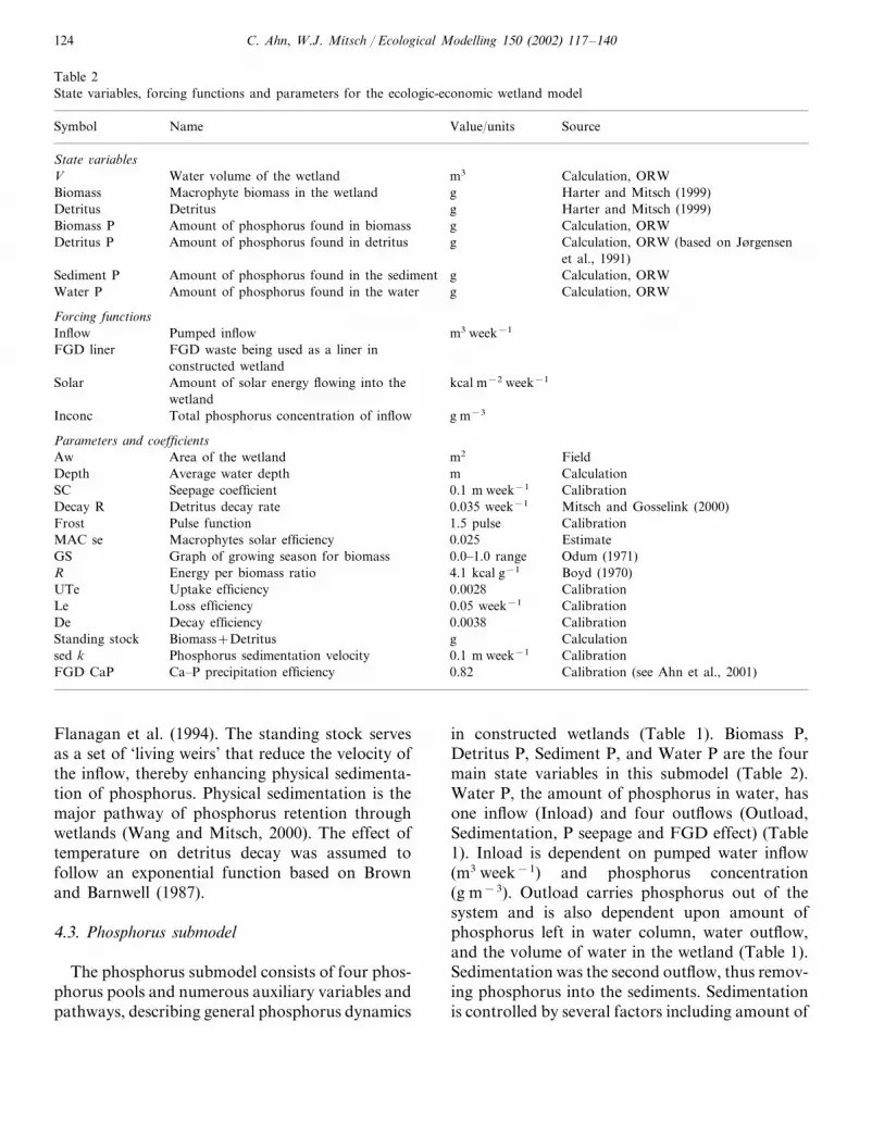
Table 2State variables, forcing functions and parameters for the ecologic-economic wetland model

Value/unitsName SourceSymbol

State �ariablesm3 Calculation, ORWV Water volume of the wetlandgMacrophyte biomass in the wetland Harter and Mitsch (1999)Biomass

DetritusDetritus g Harter and Mitsch (1999)Amount of phosphorus found in biomassBiomass P g Calculation, ORW

gAmount of phosphorus found in detritus Calculation, ORW (based on JørgensenDetritus Pet al., 1991)

Sediment P gAmount of phosphorus found in the sediment Calculation, ORWgAmount of phosphorus found in the water Calculation, ORWWater P

Forcing functionsInflow m3 week−1Pumped inflow

FGD waste being used as a liner inFGD linerconstructed wetlandAmount of solar energy flowing into theSolar kcal m−2 week−1

wetlandg m−3Inconc Total phosphorus concentration of inflow

Parameters and coefficientsArea of the wetlandAw m2 Field

mAverage water depth CalculationDepthSeepage coefficientSC 0.1 m week−1 Calibration

0.035 week−1Detritus decay rate Mitsch and Gosselink (2000)Decay RPulse functionFrost 1.5 pulse CalibrationMacrophytes solar efficiencyMAC se 0.025 Estimate

0.0–1.0 rangeGraph of growing season for biomass Odum (1971)GS4.1 kcal g−1R Boyd (1970)Energy per biomass ratio0.0028Uptake efficiency CalibrationUTe

Loss efficiencyLe 0.05 week−1 CalibrationDecay efficiencyDe 0.0038 Calibration

gBiomass+Detritus CalculationStanding stockPhosphorus sedimentation velocitysed k 0.1 m week−1 Calibration

0.82 Calibration (see Ahn et al., 2001)Ca–P precipitation efficiencyFGD CaP

Flanagan et al. (1994). The standing stock servesas a set of ‘living weirs’ that reduce the velocity ofthe inflow, thereby enhancing physical sedimenta-tion of phosphorus. Physical sedimentation is themajor pathway of phosphorus retention throughwetlands (Wang and Mitsch, 2000). The effect oftemperature on detritus decay was assumed tofollow an exponential function based on Brownand Barnwell (1987).

4.3. Phosphorus submodel

The phosphorus submodel consists of four phos-phorus pools and numerous auxiliary variables andpathways, describing general phosphorus dynamics

in constructed wetlands (Table 1). Biomass P,Detritus P, Sediment P, and Water P are the fourmain state variables in this submodel (Table 2).Water P, the amount of phosphorus in water, hasone inflow (Inload) and four outflows (Outload,Sedimentation, P seepage and FGD effect) (Table1). Inload is dependent on pumped water inflow(m3 week−1) and phosphorus concentration(g m−3). Outload carries phosphorus out of thesystem and is also dependent upon amount ofphosphorus left in water column, water outflow,and the volume of water in the wetland (Table 1).Sedimentation was the second outflow, thus remov-ing phosphorus into the sediments. Sedimentationis controlled by several factors including amount of


phosphorus in water column and the amount ofstanding stock in the wetland. Sedimentation co-efficient (sed k) was obtained through model cali-bration to find a better-fit between observed andsimulated percent TP removal. Phosphorus seep-age accounted for a certain amount of phosphoruslost from the water column through seepage, butthis term is designed to become zero when liners areused in the wetlands due to the assumption of noseepage. FGD effect was included in the model asthe fourth outflow of Water P. To simulate theenhanced P removal observed through the experi-ments by Ahn et al. (2001), approximately 10%more phosphorus (as mass) was simulated to beremoved from the water column in wetlands beingbuilt with FGD liners. A potentially negativeimpact of FGD materials on phosphorus retention,such as decreasing sedimentation by lowered stand-ing stock when FGD toxicity is active, is alsoincluded in the model. Most phosphorus used bymacrophytes is taken up from sediments (Wangand Mitsch, 2000) and is assumed to be propor-tional to net primary productivity (NPP flow) ofthe wetland macrophyte. Loss of phosphorus inbiomass to detritus, and then to the sedimentthrough decomposition processes was generallysimulated as a linear pathway. Calibration effortswere generally focused on percent phosphorusremoval prediction in constructed wetlands.

4.4. Economic accounting submodel

Two different aspects of potential cost savingfrom recycling FGD wastes as liners in constructedwetlands were explored in this submodel. One wasa cost saving from wetland construction with FGDliners relative to commonly used clay materials,which provide useful a priori information to man-agers and decision-makers on treatment wetlands.The cost of wetland construction varies widely,depending on the location, type, size, and objec-tives of the wetland (Mitsch and Gosselink, 2000).A strong relationship between wetland cost perarea and wetland size found by Mitsch and Gos-selink (2000) based on various cases of treatmentwetlands in the US, including the ORW and theLCW, was used in our economic accounting sub-model to calculate cost of wetland construction.

CA=$196 336×A−0.511 n=15 R2=0.785(1)

where CA is the capital cost of wetland constructionper unit area ($ ha−1), and A is the wetland area(ha).

Cost of liner material is generally reported tocomprise 20–25% of total wetland constructioncost (Kadlec et al., 2000). In the model, we applied20% of the total estimated cost of wetland con-struction conservatively as the potential saving ofusing FGD waste relative to clay being purchased.The capital saving of FGD liner was converted intoan annualized saving based on an assumed 8%interest rate and 30-year lifetime of a constructedwetland.

The other possible saving from using FGD wasteas a liner results from cost of phosphorus removalin constructed wetlands. Bystrom (1998) estimatednitrogen removal cost in wetlands by linking afunction for construction costs of wetlands with afunction that defines the nitrogen removal capacityof wetlands. Similarly, in our study, a possible costsaving ($ year−1) was calculated by multiplying theunit cost of removing 1 g of TP from surface inflowby the amount of phosphorus being additionallyremoved due to FGD by-product compared to clay(see Table 1).

The unit cost of phosphorus removal would bea useful tool in the development plans for a reliable,

Table 3Hydrology, phosphorus loading data (mean�S.E., (n)) forthe Olentangy River Wetland (ORW) and the Licking CountyWetland (LCW), 1996–1997

LCW northORW basin 1Parametersbasin

Area (ha) 1 3.2Inflow (m3 day−1) 932�40 (75) 3.138�127 (87)

9.8�0.40 (87)9.3�0.4 (75)Hydraulic loadingrate (cm day−1)

2.6�0.2 (87)Retention time 2.1�0.3 (75)(day)

1.19�0.15 (87)0.16�0.01 (75)Inflow Pconcentration(mg P l−1)

20�1.2 (87)38.9�1.1 (75)P removal byconcentration(%)


Table 4Simulations run of the ecologic-economic wetland model inthis study

Number ofSimulationsimulations

Calibrating model of ecosystem (phosphorus)1(1) Calibration of model with the

ORWa data in 1996–1997(2) Validation of model with the 1

LCWb data in 1996–1997

Sensiti�ity analysis (with LCW)(3) Phosphorus sedimentation coefficient 5

(sed k)(4) Interest rate and wetland life 4

expectancy5(5) Total phosphorus inflow

concentration

Simulations to design a pilot-scale wetland lined with FGD(6) Manipulating hydraulic loading 7

rate and inflow TP concentration(7 different P loading rate simulated)

Real-world application of the model with LCW(7) LCW with clay liner (no seepage) 1

1(8) LCW with FGD liner(no seepage+FGD effects)

a Olentangy River Wetland; data from ORW basin 1 wereused.

b Licking County Wetland; data from the north basin(LCWN) were used.

annualized cost for each constructed wetland calcu-lated was then divided by total annual amount ofphosphorus removed through it, thus resulting inunit cost ($) of 1 g of phosphorus removed. Valuesof all other possible services being provided byconstructed wetlands such as recreation, biodiver-sity and removal of other nutrients or pollutants,although important, are not included in this unitcost estimation. Amount of phosphorus enteringthe water column (Inload, kg-P ha−1 day−1) andTP concentration of inflow (Inconc, g m−3) werefound to be closely related to unit cost of phospho-rus removed in constructed wetlands in a previousstudy (Brown and Caldwell Consultants, 1993).Therefore, we established two power functions todescribe the relationship between unit cost andphosphorus loading in constructed wetlands:

Unit cost=0.0673×Inload(−0.8189)

n=5 R2=0.5375 (2)

Unit cost=0.1781×Inconc(−0.7151)

n=5 R2=0.9753 (3)

where Unit cost is the cost of removing 1 g of TP(US $ g-P−1), Inload is the amount of phosphorusentering the water column (kg-P ha−1 day−1), andInconc is the TP concentration of inflow (g m−3).

In the above equations, the unit cost of phospho-rus removed decreases drastically as TP inflowconcentration increases as found in Brown andCaldwell Consultants (1993). Inflow TP concentra-tion explained almost 98% of the variance of unitcost of removing 1 g of TP through constructedwetlands. Therefore, the second equation wasadopted in our model to link the phosphorussubmodel to the economic accounting submodel.

5. Results and discussion

The model was used to simulate ecologic-eco-nomic dynamics of phosphorus retention in con-structed wetlands. Table 4 summarizes simulationsperformed in this study.

5.1. Simulation results-calibration and �alidation

The process of calibration consists of adjusting

implementable treatment system at a reasonablecost. Very few studies have been conducted on howmuch it would cost to treat a unit mass of phospho-rus through wetland treatment technology. In orderto quantify the removal cost of a unit mass ofphosphorus in our study, we used data availablefrom real-world examples including North Ameri-can Wetland Database (NAWDB, 1993), ORWand LCW to obtain construction costs of thosewetlands. Those capital construction costs wereconverted into periodic series of annualized pay-ments for a 30 years period at an 8% interest rate,and then added it to annual operation and mainte-nance costs of those wetlands to calculate the totalannual costs. The calculated total annual costs wereadjusted to January 2000 by multiplying by 1.176based on Mean history cost index (Means Com-pany Inc., 1999) as most construction costs adoptedin the calculations were in 1993 dollars. The total


key model parameters so that simulated values fora modeled variable (TP outflow concentration or %TP removal) are in agreement with observed fielddata. The hydrology submodel was the first sub-model to be calibrated, and showed less than 10%difference for average surface outflow at each timestep (m3 week−1) between field data and modeloutputs. Water depth was predicted almost thesame as their field measurements for two differentsites (ORW 1:0.2 m; LCWN: 0.25 m), resulting inless than 5% difference.

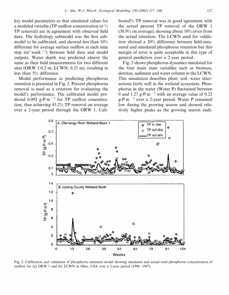
Model performance in predicting phosphorusretention is presented in Fig. 2. Percent phosphorusremoval is used as a criterion for evaluating themodel’s performance. The calibrated model pre-dicted 0.092 g-P m−3 for TP outflow concentra-tion, thus achieving 43.2% TP removal on averageover a 2-year period through the ORW 1. Cali-

brated% TP removal was in good agreement withthe actual percent TP removal of the ORW 1(38.9% on average), showing about 10% error fromthe actual retention. The LCWN used for valida-tion showed a 20% difference between field-mea-sured and simulated phosphorus retention but thismargin of error is quite acceptable in this type ofgeneral prediction over a 2-year period.

Fig. 3 shows phosphorus dynamics simulated forthe four main state variables such as biomass,detritus, sediment and water column in the LCWN.This simulation describes plant–soil–water inter-actions fairly well in the wetland ecosystem. Phos-phorus in the water (Water P) fluctuated between0 and 1.27 g-P m−2 with an average value of 0.22g-P m−2 over a 2-year period. Water P remainedlow during the growing season and showed rela-tively higher peaks as the growing season ends.

Fig. 2. Calibration and validation of phosphorus retention model showing simulated and actual total phosphorus concentration ofoutflow for (a) ORW 1 and (b) LCWN in Ohio, USA over a 2-year period (1996–1997).


Fig. 3. Simulated phosphorus dynamics in biomass, detritus, water and sediment in LCW over a 2-year period (1996–1997) in thisstudy.

Biomass production and standing stock start asthe growing season begins, which both influencesedimentation of phosphorus positively. Therefore,phosphorus in the water column is closely affectedby the macrophyte submodel, and hence shows akind of seasonality. Phosphorus in plant biomassfluctuates between about 0.03 and 2.03 g-P m−2 inthe LCW simulation seasonally because of itsdependence on the macrophyte submodel. As NPPflow increases, uptake of phosphorus from thesediment also increases (Fig. 3). The outflow path-way of biomass phosphorus is directly dependenton the loss rate of biomass to detritus in themacrophyte submodel (Table 1). Biomass P is alsoaffected greatly by the occurrence of frost whichterminates the growing season on week 41 in thefirst year and on week 93 in the second year. Thephosphorus in detritus (Detritus P) follows aninverse pattern of the phosphorus in biomass. Asbiomass P decreases on around week 41, thephosphorus flows from biomass to detritus. Phos-phorus in the sediment (Sediment P) increases overtime and reaches a peak of 76 g-P m−2 over a2-year period in the LCW, but it shows relativelylower rate of increase during the growing seasonscompared to non-growing seasons sincemacrophyte uptake of phosphorus from sedimentsdrastically increases (Fig. 3).

5.2. Sensiti�ity analysis

Fig. 4 shows how percent TP removal of wet-lands changes as phosphorus sedimentation coeffi-cient (sed k) changes. TP retention in wetlandsincreases as sed k increases, thus indicating thatphosphorus sedimentation is a significant processcontributing to phosphorus retention efficiency ofour wetland model. Inflow TP concentration wasalso varied from the inflow TP concentration of theLCWN by �2 orders of magnitude, which did notsignificantly influence percent TP removal in thewetland model when the inflow TP concentrationwas higher than 0.12 g m−3 as shown in Fig. 5.

Fig. 4. Sensitivity of percent change in total phosphorusretention to phosphorus sedimentation coefficient (sed k).


Fig. 5. Relationship of TP removal (%), unit cost of P removal, and P treatment savings along a gradient of inflow TP concentrationin the calibrated model simulating LCW in this study. Two thick, vertically dotted lines indicate minimum and maximum values ofinflow TP from North American Treatment Wetland Database (NAWDB, 1993). LCWN is Licking County Wetland North basin.Values in the boxes are mean inflow TP concentrations for LCWN and NAWDB.

Inflow TP concentration of 0.12 g m−3 is usuallyregarded a low-P condition as in the river inflow ofthe ORW (Spieles and Mitsch, 2000). Most treat-ment wetlands are found to have higher inflow TPconcentrations than 0.12 g m−3 (Kadlec andKnight, 1996). Therefore, TP retention predicted inour model may not be sensitive to change in theinflow TP concentrations of treatment wetlands.Rapidly decreasing percent TP removal was ob-served when Inflow TP concentration was below0.2 g m−3 (Fig. 5).

5.3. Simulations for the pilot-scale wetland with aFGD liner

We ran the dynamic model with a variety ofcombinations of hydraulic loading rates and inflowTP concentrations for the pilot-scale wetland (�3m×7.8 m×1.5 m) lined with FGD by-productcurrently under construction at the ORWRP. Table5 shows those simulation results. Mitsch and Gos-selink (2000) reported that loading rates to surfaceflow wetlands for wastewater treatment from small

municipalities ranged from 1.4 to 22 cm day−1

(average=5.4 cm day−1). Knight (1990) recom-mended a rate of 2.5–5 cm day−1 for surface watersystems. The rate of 5–10 cm day−1 was alsomaintained for the ORW and LCW since they wereconstructed (Spieles and Mitsch, 2000). Therefore,we chose 5 cm day−1 as target inflow loading rate,one of the design parameters for this pilot-scalewetland, and ran the model while varying the valuewithin a reasonable range from 2.5 to 15 cm day−1.Inflow TP concentration was also varied from 0.1to 10 g m−3, a reasonable value range for treatedwastewater entering constructed wetlands based onthe NAWDB (1993), while fixing the hydraulicloading rate at 5 cm day−1 to investigate thechange in phosphorus retention. As hydraulic load-ing rates increased from 2.5 to 15 cm day−1 percentP removal (on average as mass) decreased by 29%when the inflow TP concentration was consistentlykept at 2 g m−3 as shown in Table 5. Themodel estimated more than 60% phosphorusremoval consistently when inflow TP concentrationvaried from 0.1 to 10 g m−3 at 5 cm day−1


Tab

le5

Sim

ulat

ions

cond

ucte

dov

era

2-ye

arpe

riod

unde

rva

riou

sco

mbi

nati

ons

ofhy

drau

lican

dph

osph

orus

-loa

ding

rate

sto

desi

gnth

epi

lot-

scal

ew

etla

nd(�

3m

×7.

8m

×1.

5m

)lin

edw

ith

FG

Dby

-pro

duct

inth

isst

udy

Hyd

raul

iclo

adin

gP

load

ing

Sim

ulat

ion

Wat

erde

ptha

Pre

mov

al(m

ass)

Inflo

wP

conc

entr

atio

n(g

m−

3)

Ret

enti

onti

mea

(cm

day−

1)

(gm

−2

day−

1)

(day

s)(m

)(%

)

2.5

0.06

(0.1

2)2.

5(5)

20.

0574

15

0.12

2.5

20.

10.

005

633

50.

122.

52

0.1

635

0.12

2.5

43

0.15

635

50.

122.

510

0.5

636

100.

25(0

.12)

2.5(

1.3)

20.

251

150.

37(0

.12)

2.5(

0.83

)2

70.

345

aV

alue

sin

pare

nthe

ses

show

corr

espo

ndin

gch

ange

betw

een

wat

erde

pth

and

rete

ntio

nti

me.


of hydraulic loading rate (Table 5). Most simula-tions predicted more than 50% TP retention ex-cept the case where the hydraulic loading rate was15 cm day−1 and inflow TP concentration was 2g m−3. Mean TP retention over a 2-year run ofthe model in this case was less than 50%, thusindicating hydraulic loading rate is the majordeterminant of phosphorus retention performancepredicted by the model.

Retention time in Table 5 was calculated by asimple theoretical equation below (Mitsch andGosselink, 2000).

t=Vp/Q (4)

where t is the theoretical retention time (day), V isthe volume of water for surface flow wetland (m3),P is the porosity of medium, and �1.0 for sur-face flow wetlands, Q is the flow rate throughwetland (m3 day−1) = (Qi+Qo)/2, where Qi isthe inflow and Qo is the outflow.

Manipulating water depth can change calcu-lated retention time. The pilot-scale FGD-linedwetlands are designed to control water depth sothat we can change the retention time of waterbeing treated in the wetlands. The values in paren-theses in Table 5 for water depth and retentiontime show those possible changes. Based on thosesimulations explored we suggested design parame-

Fig. 6. STELLA™ diagram of the ecologic-economic model.


Fig. 6. (Continued)

ters for the pilot-scale experimental wetlands(Table 6). We chose 5 cm days−1 as a conserva-tive loading rate and 2–3 g m−3 typical of treatedwastewater as inflow TP concentration. Waterdepth is designed up to 0.3 m in the pilot-scalewetland (Table 6), high enough to contain otheraquatic life than just macrophytes, e.g. amphibi-ans and benthic invertebrates.

5.4. Simulation of LCW with a liner

Table 7 shows the model simulations of LCWNwith two different types of liners, either clay orFGD by-product. The same hydraulic loading

rate (9.8 cm day−1) and inflow TP concentration(1.19 g m−3) as in the model validation wereapplied to those simulations. The differences fromthe validation simulation was no seepage effect inboth simulations of LCWN with an either clay ora FGD liner. Moreover, additional P retentionand early phytotoxicity from FGD by-productwere applied to the model simulation with a FGDliner. A slight increase of water depth was ob-served in the simulations with a liner due to noseepage (Table 7). The no seepage effect includedin the model simulation with an either clay orFGD liner resulted in more phosphorus in thewater column of the LCW, thus potentially de-


creasing phosphorus retention since no morephosphorus could be removed through seepage(see Table 1). Based on this model structure, theLCW with a clay liner showed a slight decrease in

its phosphorus retention relative to that with noliner (Table 7). More investigation is needed onthe physicochemical properties of clay liner mate-rial being used for treatment wetlands. The pilot-

Fig. 6. (Continued)


Fig. 6. (Continued)

scale wetlands lined with clay as a control to theFGD-lined ones may provide further informationto be incorporated into the model as the experi-ment proceeds.

In the simulation of LCW with a FGD linersome changes of P dynamics were found com-pared to the simulation conducted without aFGD liner. Most importantly, biomass produc-tion was about 9% lower on average due topotential phytotoxicity applied in the model. Thistrend was much pronounced in the first year,showing about 14% lower biomass production astoxicity was modeled to mitigate over time andbecome negligible toward the end of the first year.

Phosphorus in the biomass (Biomass P) was also9% lower than that in the simulation with noliner. Reduction in biomass production naturallyinduced a decrease in detritus by an average of12%. As a result, standing stock, biomass plusdetritus, showed a 10% decrease on average overa 2-year period, which may have influenced phos-phorus retention performance of the wetland be-cause the standing stock was modeled to influencephosphorus sedimentation. Higher percent TP re-movals both by concentration and by mass, how-ever, were observed in the LCW simulated with aFGD liner compared to other simulations (Table7). Amount of phosphorus in water column (Wa-


Table 6Design parameters suggested for the pilot-scale FGD wetlands(�3 m×7.8 m×1.5 m) at the Olentangy River WetlandResearch Park (ORWRP)

Parameters Suggested design

Surface flowType of flowHydrology

Loading 5 cm days−1 (for�50% TP removal)Retention time �1 day

0.1–0.3 mWater depth2–3 g m−3Phosphorus

loadingBasin characteristics

Multiple (4)Cells (number)Planting material Scirpus sp.Substrate material On-site soil over FGD by-product

Table 8Potential liner cost saving by recycling FGD by-product rela-tive to clay as a liner in the Licking County Wetland (LCW)under various combinations of interest rate and life expectancy

Interest rate Liner cost saving (US $Life of wetlandha−1 year−1)(years) (%)

135183030 6 1105

10 1613301549820

8 127540

about US $ 1400 ha−1 years−1for the LCW(Table 8). A model equation calculating the costof wetland construction is a function of wetlandsize, therefore the liner cost saving (20% of wet-land construction cost assumed) will decrease pro-portionately to decreasing construction cost as thewetland being built gets bigger, following theso-called ‘economy of scale’. Liner costs in gen-eral are variable, based on the quantity, thicknessand type of material specified (Kadlec et al.,2000). The scenario tested above was based on theassumption that we would not find on-site soilswith high-clay content suitable for use as a liner.However, our approach remains reasonable andpractical even at sites that do have high-clay soils.Kadlec and Knight (1996) report that cost oftesting and compaction, even with good soils inplace, can exceed the costs of a 0.08-cm polyvinylchloride (PVC) liner.

Sensitivity of liner cost saving to the choice ofinterest rate and life expectancy of the wetlandsystem was also explored (Table 8). If a 6%interest rate were chosen instead of 8%, then theannualized cost saving of the liner would be18.2% less or about US $ 1100 ha−1 year−1. If a

ter P) showed a 10% additional decrease as aresult of potentially enhanced Ca–P precipitationincluded in the simulation. Therefore, model pre-dictions show that increased phosphorus retentionefficiency by FGD by-products offset the initialphytotoxicity that could otherwise negatively infl-uence phosphorus retention.

5.5. Economic estimations

Recycling FGD by-products in wetland treat-ment systems offers two possible cost savings;savings from both liner cost and phosphorus re-moval cost. Liner cost saving was estimated in theeconomic accounting submodel. This estimationpresents only the cost of material for a liner,excluding cost for excavation and compactionprocedures needed to install the liner. Based onthe 30-year, 8% interest assumption, calculationwith the model resulted in the liner cost saving of

Table 7Mean water depth and phosphorus retention of the Licking County Wetland (LCW) with two different types of potential liner, clayand FGD by-product, over a 2-year period of model simulation

Simulation P removal (concentration) (%)Water depth (m) P removal (mass) (%)

0.25No linera 24.8 34.721.923.20.27Clay liner

0.27FGD liner 32.9 37.3

a The case of validation.


10% interest rate were applied, the cost savingwould be 16.3% more or about US $ 1600ha−1 year−1. At a fixed 8% rate, decreasing thelife expectancy of the wetland from 30 years to 20years resulted in about 13% increase in the annu-alized cost saving, while increasing it to 40 yearsdecreased the cost saving by about 6%. Therefore,it seems that the liner cost saving is sensitive toassumptions regarding interest rate and life expec-tancy of wetlands.

Fig. 5 combines the other potential cost saving,P treatment saving, with both percent phosphorusremoval predicted by the model and unit cost of Premoval along a gradient of inflow TP concentra-tions. P treatment saving relates closely withinflow TP concentration (r2=0.9944) and in-creases as the TP concentration of surface inflowincreases (Fig. 5). P treatment saving can poten-tially get bigger than the liner cost saving withincreasing TP inflow concentration, coveringmore than half of the total potential cost saving(Table 9). Two vertically dotted lines in Fig. 5show the minimum and maximum values ofinflow TP concentration observed for treatmentwetlands in North America (NAWDB, 1993),showing how much saving can be possible in theLCW when the inflow TP concentration changeswithin that range. Table 9 presents total potentialcost saving estimated from the FGD-lined LCW(6.4 ha), which was about US $ 23 000 per year(US $ 3552 ha−1 year−1×6.4 ha) by the model.

6. Conclusions

Recycling FGD by-products as liners in con-structed wetlands may be environmentally benefi-

cial and potentially economical. As long as wehave to haul liner material to the site where thewetland treatment system is being constructed,FGD wastes provide an economic edge over clayor commercial liner materials. Enhanced phos-phorus retention consistently applied in the modelsimulations through this study, however, needsmore verification since it was based on the short-term, small-scale mesocosm studies. Therefore, re-cycling FGD wastes may or may not be as mucheconomically feasible or cost-effective as projectedin our study. A larger-scale, long-term wetlandstudy with FGD wastes is currently underway toobtain more data, which may lead to better mani-festation and applicability of our ecologic-eco-nomic model. Further studies of phosphorusdynamics in FGD-lined wetlands and full socio-economic assessment of recycling FGD wastes intreatment wetlands are still needed. The uniqueecologic-economic modeling approach taken inthis study is nonetheless valid and provides abridge between wetland ecology and economicaspects of recycling FGD wastes in constructedwetlands.

Acknowledgements

This research was supported by the Ohio CashDevelopment Office within the Ohio Departmentof Development, Olentangy River Wetland Re-search Park Publication 02-602.

Appendix A. STELLA™ equations of theecologic-economic model (Fig. 6)

Hydrology SubmodelV(t)=V(t−dt)+(Inflow−Outflow−Seepage)*dtINIT V=8000

INFLOWS:Inflow=HydroinflowOUTFLOWS:Outflow=(2.1e−4*V �2)+(0.6*V)Seepage=IF(FGD – factor=1) THEN(0)ELSE(V*SC/depth)

Table 9Potential total cost saving of recycling FGD as a liner in theLicking County Wetland (LCW; 6.4 ha) predicted by thesimulation model over a 2-year run in this study

Total cost savingP treatment savingLiner cost savinga

(US $ year−1)(US $ year−1) (US $ year−1)

8646 14 086 22 732

a Based on the 30 year, 8% interest assumption.


Aw=32000depth=V/AwSC=0.1Tr=V/((Inflow+Outflow)/2)*7Hydroinflow=GRAPH(TIME)(1.00, 21969),(2.00, 21969), (3.00, 17010), (4.00, 21969), (5.00,21969), (6.00, 17143), (7.00, 14651), (8.00,21969), (9.00, 19901), (10.0, 20881), (11.0,27293), (12.0, 22442), (13.0, 12642), (14.0,12747), (15.0, 23555), (16.0, 43190), (17.0,7763), (18.0, 40012), (19.0, 26390), (20.0,13223), (21.0, 12054), (22.0, 18151), (23.0,21175), (24.0, 17115), (25.0, 15022), (26.0,15981), (27.0, 13328), (28.0, 19425), (29.0,24458), (30.0, 23849), (31.0, 20216), (32.0,15022), (33.0, 13566), (34.0, 16058), (35.0,15498), (36.0, 14735), (37.0, 17171), (38.0,13699), (39.0, 11445), (40.0, 16933), (41.0,13146), (42.0, 14469), (43.0, 15953), (44.0,14812), (45.0, 15582), (46.0, 16401), (47.0,21969), (48.0, 20006), (49.0, 22869), (50.0,27741), (51.0, 21969), (52.0, 21969), (53.0,20405), (54.0, 19768), (55.0, 27664), (56.0,26607), (57.0, 39004), (58.0, 24297), (59.0,25970), (60.0, 21462), (61.0, 36967), (62.0,28063), (63.0, 30814), (64.0, 28567), (65.0,23821), (66.0, 22470), (67.0, 24010), (68.0,21861), (69.0, 24353), (70.0, 25011), (71.0,27216), (72.0, 23926), (73.0, 23184), (74.0,33810), (75.0, 20167), (76.0, 67942), (77.0,20272), (78.0, 19971), (79.0, 19971), (80.0,19971), (81.0, 9151), (82.0, 18969), (83.0,10166), (84.0, 6466), (85.0, 8922), (86.0, 19971),(87.0, 23957), (88.0, 22183), (89.0, 20655), (90.0,23640), (91.0, 23957), (92.0, 27749), (93.0,22389), (94.0, 25021), (95.0, 19856), (96.0,20354), (97.0, 31724), (98.0, 28642), (99.0,31724), (100, 35630), (101, 25021), (102, 19971),(103, 37700), (104, 32891)

Macrophyte SubmodelBiomass(t)=Biomass(t−dt)+(NPP–flow–Loss)*dtINIT Biomass=950000

INFLOWS:NPP– flow=Solar*MAC–se*GS*FGDtf/

R*AwOUTFLOWS:Loss=Biomass*(0.0007+frost)Detritus(t)=Detritus(t−dt)+(Loss−Decay)*dtINIT Detritus=1100000

INFLOWS:Loss=Biomass*(0.0007+frost)OUTFLOWS:Decay=Detritus*Decay–R*FTDecay–R=0.035FGDtf=IF(FGD–factor=1) THEN(Tx)ELSE(1)frost=PULSE(1.5, 41, 52)FT=1.06�(Wtemp-20)MAC–se=0.025R=4.1Solar=4000-2000*COS(2*PI*(TIME)/52)Standing–Stock=Biomass+DetritusWtemp=15-13*COS(2*PI*(TIME)/52)GS=GRAPH(TIME)(1.00, 0.00), (2.00, 0.00), (3.00, 0.00), (4.00,0.00), (5.00, 0.00), (6.00, 0.00), (7.00, 0.00),(8.00, 0.00), (9.00, 0.00), (10.0, 0.00), (11.0,0.00), (12.0, 0.00), (13.0, 1.00), (14.0, 1.00),(15.0, 1.00), (16.0, 1.00), (17.0, 1.00), (18.0,1.00), (19.0, 1.00), (20.0, 1.00), (21.0, 1.00),(22.0, 1.00), (23.0, 1.00), (24.0, 1.00), (25.0,1.00), (26.0, 1.00), (27.0, 1.00), (28.0, 1.00),(29.0, 1.00), (30.0, 1.00), (31.0, 1.00), (32.0,1.00), (33.0, 1.00), (34.0, 1.00), (35.0, 1.00),(36.0, 1.00), (37.0, 1.00), (38.0, 1.00), (39.0,0.00), (40.0, 0.00), (41.0, 0.00), (42.0, 0.00),(43.0, 0.00), (44.0, 0.00), (45.0, 0.00), (46.0,0.00), (47.0, 0.00), (48.0, 0.00), (49.0, 0.00),(50.0, 0.00), (51.0, 0.00), (52.0, 0.00), (53.0,0.00), (54.0, 0.00), (55.0, 0.00), (56.0, 0.00),(57.0, 0.00), (58.0, 0.00), (59.0, 0.00), (60.0,0.00), (61.0, 0.00), (62.0, 0.00), (63.0, 0.00),(64.0, 0.00), (65.0, 1.00), (66.0, 1.00), (67.0,1.00), (68.0, 1.00), (69.0, 1.00), (70.0, 1.00),(71.0, 1.00), (72.0, 1.00), (73.0, 1.00), (74.0,1.00), (75.0, 1.00), (76.0, 1.00), (77.0, 1.00),(78.0, 1.00), (79.0, 1.00), (80.0, 1.00), (81.0,1.00), (82.0, 1.00), (83.0, 1.00), (84.0, 1.00),(85.0, 1.00), (86.0, 1.00), (87.0, 1.00), (88.0,1.00), (89.0, 1.00), (90.0, 1.00), (91.0, 0.00),


(92.0, 0.00), (93.0, 0.00), (94.0, 0.00), (95.0,0.00), (96.0, 0.00), (97.0, 0.00), (98.0, 0.00),(99.0, 0.00), (100, 0.00), (101, 0.00), (102, 0.00),(103, 0.00), (104, 0.00)Tx=GRAPH(TIME)(1.00, 0.8), (2.00, 0.8), (3.00, 0.8), (4.00, 0.8),(5.00, 0.8), (6.00, 0.8), (7.00, 0.8), (8.00, 0.8),(9.00, 0.8), (10.0, 0.8), (11.0, 0.8), (12.0, 0.8),(13.0, 0.8), (14.0, 0.8), (15.0, 0.8), (16.0, 0.8),(17.0, 0.8), (18.0, 0.8), (19.0, 0.8), (20.0, 0.8),(21.0, 0.8), (22.0, 0.808), (23.0, 0.816), (24.0,0.824), (25.0, 0.832), (26.0, 0.84), (27.0, 0.848),(28.0, 0.852), (29.0, 0.86), (30.0, 0.868), (31.0,0.876), (32.0, 0.884), (33.0, 0.892), (34.0, 0.9),(35.0, 0.908), (36.0, 0.916), (37.0, 0.924), (38.0,0.932), (39.0, 0.94), (40.0, 0.948), (41.0, 0.952),(42.0, 0.96), (43.0, 0.968), (44.0, 0.976), (45.0,0.984), (46.0, 0.992), (47.0, 1.00), (48.0, 1.00),(49.0, 1.00), (50.0, 1.00), (51.0, 1.00), (52.0,1.00), (53.0, 1.00), (54.0, 1.00), (55.0, 1.00),(56.0, 1.00), (57.0, 1.00), (58.0, 1.00), (59.0,1.00), (60.0, 1.00), (61.0, 1.00), (62.0, 1.00),(63.0, 1.00), (64.0, 1.00), (65.0, 1.00), (66.0,1.00), (67.0, 1.00), (68.0, 1.00), (69.0, 1.00),(70.0, 1.00), (71.0, 1.00), (72.0, 1.00), (73.0,1.00), (74.0, 1.00), (75.0, 1.00), (76.0, 1.00),(77.0, 1.00), (78.0, 1.00), (79.0, 1.00), (80.0,1.00), (81.0, 1.00), (82.0, 1.00), (83.0, 1.00),(84.0, 1.00), (85.0, 1.00), (86.0, 1.00), (87.0,1.00), (88.0, 1.00), (89.0, 1.00), (90.0, 1.00),(91.0, 1.00), (92.0, 1.00), (93.0, 1.00), (94.0,1.00), (95.0, 1.00), (96.0, 1.00), (97.0, 1.00),(98.0, 1.00), (99.0, 1.00), (100, 1.00), (101, 1.00),(102, 1.00), (103, 1.00), (104, 1.00)

Phosphorus SubmodelBiomass–P(t)=Biomass–P(t−dt)+(Uptake–Loss–P)*dtINIT Biomass–P=1430

INFLOWS:Uptake=NPP– flow*UTeOUTFLOWS:Loss–P=Le*LossDetritus–P(t)=Detritus–P(t−dt)+(Loss–P−Decomp–P)*dtINIT Detritus–P=9400

INFLOWS:Loss–P=Le*LossOUTFLOWS:Decomp–P=Decay*DeSediment–P(t)=Sediment–P(t−dt)+(Decomp–P+ST-Uptake)*dtINIT Sediment–P=1920000

INFLOWS:Decomp–P=Decay*DeST=IF(Standing–Stock�4000000)THEN(Water–P*sed–k/depth)ELSE((Standing–Stock*0.000000005+sed–k)/depth*Water–P)OUTFLOWS:Uptake=NPP– flow*UTeWater–P(t)=Water–P(t-dt)+(Inload-Outload-ST-FGD–effect-P–seepage)*dtINIT Water–P=9600

INFLOWS:Inload=Inflow*In–ConcOUTFLOWS:Outload=Water–P*Outflow/VST=IF(Standing–Stock�4000000)THEN(Water–P*sed–k/depth)ELSE((Standing–Stock*0.000000005+sed–k)/depth*Water–P)FGD–effect=IF(FGD–factor=1) THEN(Water–P*FGD–CaP) ELSE(0)P–seepage=IF(FGD–factor=1)THEN(0) ELSE(Seepage*(In–Conc+Out–conc)/2)De=0.0038FGD–CaP=0.82FGD–factor=2In–Conc=TP–in–observedLe=0.05Out–conc=Water–P/VP–removal–conc=(In–Conc-Out–conc)/In–Conc*100P–removal–load=(Inload-Outload)/Inload*100P–removed–with–clay=(Inload-Outload)P–removed–with–FGD=(Inload-Outload)*1.1sed–k=0.1


UTe=0.0028TP–in–observed=GRAPH(TIME)(1.00, 1.19), (2.00, 1.19), (3.00, 2.15), (4.00,1.19), (5.00, 1.19), (6.00, 1.75), (7.00, 1.63),(8.00, 1.19), (9.00, 0.8), (10.0, 0.62), (11.0, 2.19),(12.0, 0.34), (13.0, 11.9), (14.0, 0.36), (15.0,2.72), (16.0, 0.46), (17.0, 0.12), (18.0, 0.2), (19.0,0.18), (20.0, 0.44), (21.0, 1.19), (22.0, 1.19),(23.0, 1.19), (24.0, 1.19), (25.0, 1.19), (26.0,1.19), (27.0, 1.19), (28.0, 1.19), (29.0, 1.38),(30.0, 0.947), (31.0, 1.02), (32.0, 1.62), (33.0,1.58), (34.0, 1.08), (35.0, 0.916), (36.0, 0.541),(37.0, 1.42), (38.0, 1.56), (39.0, 1.97), (40.0,1.82), (41.0, 2.32), (42.0, 1.98), (43.0, 1.30),(44.0, 2.30), (45.0, 1.60), (46.0, 2.90), (47.0,1.19), (48.0, 0.88), (49.0, 1.50), (50.0, 1.00),(51.0, 1.19), (52.0, 1.19), (53.0, 1.30), (54.0,2.00), (55.0, 2.09), (56.0, 2.09), (57.0, 2.43),(58.0, 0.68), (59.0, 1.60), (60.0, 2.09), (61.0, 0.2),(62.0, 0.247), (63.0, 0.79), (64.0, 1.73), (65.0,0.43), (66.0, 0.57), (67.0, 0.56), (68.0, 1.71),(69.0, 0.79), (70.0, 0.2), (71.0, 0.3), (72.0, 0.98),(73.0, 0.75), (74.0, 1.19), (75.0, 0.849), (76.0,1.75), (77.0, 0.265), (78.0, 0.328), (79.0, 0.371),(80.0, 0.343), (81.0, 0.877), (82.0, 0.139), (83.0,0.25), (84.0, 0.0714), (85.0, 0.156), (86.0, 0.275),(87.0, 0.391), (88.0, 2.02), (89.0, 1.11), (90.0,1.39), (91.0, 1.58), (92.0, 0.728), (93.0, 0.447),(94.0, 1.32), (95.0, 0.462), (96.0, 0.368), (97.0,1.53), (98.0, 2.39), (99.0, 0.786), (100, 0.637),(101, 0.967), (102, 0.166), (103, 0.11), (104,0.447)TP–out–observed=GRAPH(TIME)(1.00, 0.952), (2.00, 0.952), (3.00, 0.68), (4.00,0.952), (5.00, 0.952), (6.00, 0.952), (7.00, 2.37),(8.00, 0.952), (9.00, 0.952), (10.0, 0.77), (11.0,1.02), (12.0, 0.84), (13.0, 1.04), (14.0, 0.29),(15.0, 0.11), (16.0, 0.51), (17.0, 0.952), (18.0,0.74), (19.0, 0.37), (20.0, 0.19), (21.0, 0.4), (22.0,1.84), (23.0, 1.43), (24.0, 0.952), (25.0, 0.952),(26.0, 0.952), (27.0, 0.952), (28.0, 0.952), (29.0,0.952), (30.0, 0.952), (31.0, 0.482), (32.0, 1.01),(33.0, 1.36), (34.0, 1.21), (35.0, 1.92), (36.0,4.10), (37.0, 1.09), (38.0, 0.837), (39.0, 0.952),(40.0, 0.952), (41.0, 0.952), (42.0, 0.952), (43.0,0.952), (44.0, 0.952), (45.0, 1.10), (46.0, 1.30),(47.0, 0.952), (48.0, 0.952), (49.0, 0.55), (50.0,1.20), (51.0, 0.952), (52.0, 0.952), (53.0, 1.20),

(54.0, 2.20), (55.0, 1.76), (56.0, 1.08), (57.0,1.83), (58.0, 0.75), (59.0, 1.31), (60.0, 1.70),(61.0, 0.93), (62.0, 0.673), (63.0, 4.87), (64.0,0.82), (65.0, 0.85), (66.0, 0.49), (67.0, 0.93),(68.0, 1.32), (69.0, 1.13), (70.0, 0.83), (71.0,0.23), (72.0, 1.09), (73.0, 0.9), (74.0, 0.37), (75.0,0.365), (76.0, 2.56), (77.0, 0.51), (78.0, 0.489),(79.0, 0.53), (80.0, 0.39), (81.0, 0.406), (82.0,0.883), (83.0, 0.201), (84.0, 0.724), (85.0, 0.603),(86.0, 0.214), (87.0, 0.405), (88.0, 0.374), (89.0,0.37), (90.0, 0.532), (91.0, 0.634), (92.0, 1.24),(93.0, 0.972), (94.0, 0.395), (95.0, 0.621), (96.0,0.605), (97.0, 0.551), (98.0, 1.12), (99.0, 0.789),(100, 0.675), (101, 0.201), (102, 1.15), (103,0.253), (104, 0.425)

Economic Accounting SubmodelCost–for–wetland–construction=196336*(Wt–area)

�(-0.511)*Wt–areaCWC–with–FGD=Cost–for–wetland–construction-liner–costInterest–rate=0.08liner–cost=Cost–for–wetland–construction*0.2Liner–cost–saving=-PMT(Interest–rate,NY,Liner–saving–1,0)Liner–saving–1=Cost–for–wetland–construction-CWC–with–FGDNY=30P–treatment–saving=(P–removed–with–FGD-P–removed–with–clay)*Unit–cost–of–P–wetland*52*2total–savings=Liner–cost–saving+P–treatment–savingUnit–cost–of–P–wetland=0.1781*In–Conc

�(-0.7151)Wt–area=6.4

References

Ahn, C., Mitsch, W.J., 2001. Chemical analysis of soil andleachate from experimental wetland mesocosms lined withcoal combustion products. J. Environ. Qual. 30, 1457–1463.

Ahn, C., Mitsch, W.J., Wolfe, W.E., 2001. Effects of recycledFGD liner on water quality and macrophytes of constructedwetlands: a mesocosm experiment. Water Res. 35 (3),633–642.


American Coal Ash Association Survey, 1997. 1996 CoalCombustion Product (CCP) Production and Use, AmericanCoal Ash Association, Alexandria, VA.

Baker, K.A., Fennessy, M.S., Mitsch, W.J., 1991. Designingwetlands for controlling coal mine drainage: an ecologic-eco-nomic modelling approach. Ecol. Econ. 3, 1–24.

Boyd, C.E., 1970. Amino acid, protein, and caloric content ofvascular aquatic macrophytes. Ecology 51, 902–906.

Breaux, A., Farber, S., Day, J., 1995. Using natural coastalwetlands systems for wastewater treatment: an economicbenefit analysis. J. Environ. Manag. 44, 285–291.

Brown, L.C., Barnwell Jr., T.O., 1987. The enhanced streamwater quality models QUAL2E and QUAL2E-UNCAS:documentation an user manual, EPA/600/3-87/007.

Brown and Caldwell Consultants, 1993. Everglades ProtectionProject, PHASE II Evaluation of Alternative TreatmentTechnologies, Final Draft Report, Mock, Roos and Associ-ates, Inc.

Bystrom, O., 1998. The nitrogen abatement cost in wetlands.Ecol. Econ. 26, 321–331.

Cardoch, L., Day, J.W. Jr., Rybczyk, J.M., Kemp, G.P., 2000.An economic analysis of using wetlands for treatment ofshrimp processing wastewater—a case study in Dulac, LA.Ecol. Econ. 33, 93–101.

Flanagan, N.E., Mitsch, W.J., Beach, K., 1994. Predicting metalretention in a constructed mine drainage wetland. Ecol. Eng.3, 135–159.

Grant, W.E., Thompson, P.B., 1997. Integrated ecologicalmodels: simulation of socio-cultural constraints on ecologicaldynamics. Ecol. Model. 100, 43–59.

Harter, S.K., Mitsch, W.J., 1999. Patterns of short-term sedimen-tation in a freshwater created marsh. In: Mitsch, W.J.,Bouchard, V. (Eds.), Olentangy River Wetland ResearchPark at The Ohio State University, Annual Report 1998, TheOhio State University, Columbus, Ohio, pp. 95–112.

Jørgensen, S.E., 1988. Fundamentals of Ecological Modelling.Elsevier, Amsterdam.

Jørgensen, S.E., Nielsen, S.R., Jørgensen, L.A., 1991. Handbookof Ecological Parameters and Ecotoxicology. Elsevier, Am-sterdam.

Kadlec, R.H., 1997. An autobiotic wetland phosphorus model.Ecol. Eng. 8, 145–172.

Kadlec, R.H., Hammer, D.E., 1988. Modeling nutrient behaviorin wetlands. Ecol. Mod. 40, 37–66.

Kadlec, R.H., Knight, R.L., 1996. Treatment Wetlands. CRCPress, Boca Raton, FL.

Kadlec, R.H., Knight, R.L., Vymazal, J., Brix, H., Cooper, P.,Haberl, R., 2000. Constructed Wetlands for Pollution Con-trol: Process, Performance, Design and Operation. IWAPublishing, London, England.

Knight, R.L., 1990. Wetland systems, in Natural Systems forWastewater Treatment, Manual of Practice FD-16, WaterPollution Control Federation, Alexandria, VA, pp. 211–260.

Means Company Inc., 1999. Heavy Construction Cost Data:2000, R.S. Means Company Inc., Kingston, MA.

Mitsch, W.J., Metzker, K., 1996. Tertiary treatment of wastew-ater in southwest Licking County, Ohio, with a constructedwetland. Report to Southwest Licking County CommunityWater and Sewer District, The Ohio State University,Columbus, OH.

Mitsch, W.J., Reeder, B.C., 1991. Modeling nutrient retentionof a freshwater coastal wetland: estimating the roles ofprimary productivity, sedimentation, resuspension and hy-drology. Ecol. Mod. 54, 154–187.

Mitsch, W.J., Gosselink, J.G., 2000. Wetlands, 3rd ed. Wiley,New York.

Mitsch, W.J., Wu, X., Nairn, R.W., Weihe, P.E., Wang, N., Deal,R., Boucher, C.E., 1998. Creating and restoring wetlands:a whole ecosystem experiment in self-design. BioScience 48,1019–1030.

Nairn, R.W., Mitsch, W.J., 2000. Phosphorus removal in createdwetland ponds receiving river overflow. Ecol. Eng. 14,107–126.

NAWDB, 1993. North American Treatment Wetland Database.Electronic database created by R. Knight, R. Ruble, R.Kadlec, S. Reed for the United States EnvironmentalProtection Agency, Copies available from Don Brown,USEPA, Tel.: +1-513-569-7630.

Odum, E.P., 1971. Fundamentals of Ecology. Saunders, Philadel-phia, PA.

Richardson, C.J., 1985. Mechanisms controlling phosphorusretention capacity in freshwater wetlands. Science 228,1424–1427.

Richardson, C.J., Qian, S., Craft, C.B., Qualls, R.G., 1997.Predictive models for phosphorus retention in wetlands. Wetl.Ecol. Manag. 4, 159–175.

Richmond, B., Peterson, S., 1997. STELLA V: tutorials andtechnical documentation, High Performance Systems Inc.,Hanover, New Hampshire.

Robles-Diaz-de-Leon, L.F., Nava-Tudela, A., 1998. Playing withAsimina triloba (pawpaw): a species to consider whenenhancing riparian forest buffer systems with non-timberproducts. Ecol. Mod. 112, 169–193.

Spieles, D.J., Mitsch, W.J., 2000. The effects of season andhydrologic and chemical loading on nitrate retention inconstructed wetlands: a comparison of low- and high nutrientriverine systems. Ecol. Eng. 14, 77–91.

Wang, N., Mitsch, W.J., 2000. A detailed ecosystem model ofphosphorus dynamics in created riparian wetlands. Ecol.Mod. 126, 101–130.

Wolfe, W.E., Butalia, T.S., Mitsch, W.J., Whitlatch, E., 2000.Use of Clean Coal Technology By-product in the Construc-tion of Low Permeability Liners, Technical Report, Draft,Dept. of Civil and Environmental Engineering and GeodeticScience and School of Natural Resources, The Ohio StateUniversity, Columbus, OH.

Documents

Evaluating the use of recycled coal combustion products in constructed wetlands: an ecologic-economic modeling approach