Embed Size (px)
Citation preview

v. 2.0
Interim Conservation
Framework 2019-2020
Evaluation, Measurement
and Verification Protocols
and Requirements V3.0
Interim Framework 2019-2020 April 1, 2019

The Evaluation, Measurem ent and Verificat ion (EM&V) Protocols and Requirem ents V3.0
consists of three volum es:
Volum e I : EM&V Protocols and Requirem ents
Part 1 – Developin g, Procurin g and Report in g on Evaluations (Audience : Evaluation
Administ rat ors)
Part 2 – Conductin g Evaluations (Audien ce: Evaluation Contract ors)
Volum e II : Protocols for Evaluatin g Behavioral Progra m s
Volum e III : CVR Impact Evaluation Protocols
Preface

The Independ ent Electricit y System Operator (IESO) would like to recogn iz e the Efficiency
Valuation Organizat ion (EVO) who develop ed the Internationa l Performan ce Measurem ent &
Verification Protocol (IPMVP). Their work serves as a valuable reference and foundation upon
which the ‚EM&V Protocols and Requirements V3.0‛ are developed.
Readers wishing more information on program evaluation methods can access the library of materials
available from the US Departm ent of Energy and the Office of Energy Efficiency and Renewa ble
Energy at: https://www.energy.gov/eere/analysis/program-evaluation
Acknowledgements

Preface ........................................................................i Acknow ledgements .................................................... ii
Table of Contents ...................................................... iii
Tables and Figures ....................................................iv
Abbreviations............................................................. v
Introduction................................................................vi
Part 1:
Developing, Procuring and
Reporting on Evaluations..................................... 1
Audience: Ev aluation Contractors
Part 2:
Conducting Evaluations ..................................... 43
Audience: Ev aluation Contractors
Introduction to Part 1 ................................................. 2
Step 1:
Document Market Strategy and Program Offer.......... 4
Step 2:
Anticipate Program Cause and Effect........................ 7
Step 3:
Properly Scope Program Evaluation........................ 12
Step 4:
Identify Analytical Approaches to Address Research
Questions ................................................................ 15
Step 5:
Specify Evaluation Deliverables............................... 18
Step 6:
Evaluation Classif ication Protocols .......................... 22
Step 7:
Evaluation Plan Development Guidelines ................ 26
Step 8:
Hire Independent, Qualif ied Evaluation
Contractors .............................................................. 32
Step 9:
Vendor Selection Process Guidelines...................... 34
Step 10:
Coordinate EM&V Activities and Report Findings ..... 36
Step 11:
Publication of Evaluation Reports ............................ 38
Step 12:
Guideline for Managing Program Evaluation
Contractors .............................................................. 41
Introduction to Part 2 ............................................... 44
Technical Guide 1:
Using Measures and Assumptions Lists .................. 45
Technical Guide 2:
Cost-Effectiveness Guidelines ................................. 49
Technical Guide 3:
Process Evaluation Guidelines ................................ 50
Technical Guide 4:
Project-Level Energy Savings Guidelines ................ 54
Technical Guide 5:
Gross Energy Savings Guidelines ........................... 69
Technical Guide 6:
Demand Savings Calculation Guidelines ................. 75
Technical Guide 7:
Market Effects Guidelines........................................ 80
Technical Guide 8:
Net-To-Gross Adjustment Guidelines ...................... 83
Technical Guide 9:
Guideline for Statistical Sampling and Analysis....... 89
Technical Guide 10:
Behaviour-Based Evaluation Protocols.................... 95
Glossary of General Program
Evaluation Terminology ........................................... 97
Bibliography........................................................... 103

Figures
Figure 1.0: The Basic Elements of a Logic Model ..............................................................................................10
Figure 2.0: Prescriptive Projects.........................................................................................................................59
Figure 3.0: Custom projects: equipment retrofit only ..........................................................................................61
Figure 4.0: Custom projects: operational change only 1 (demand (kW) incentives)...........................................63
Figure 5.0: Custom projects: operational change only 2 (energy (kWh) incentives) ...........................................64
Figure 6.0: Custom projects: equipment retrofit and operational changes..........................................................66
Figure 7.0: Custom projects: multiple energy conservation measures (ECMs) ..................................................67
Tables
Table 1.0: IESO EM&V standard definition for Peak..........................................................................................76
Table 2.0: Alternative definition of Peak ............................................................................................................77
Table 3.0: Sample free ridership survey question matrix...................................................................................86
Table 4.0: Common Statistical Tests for Normally Distributed Populations .......................................................94
Tables and Figures

CDM Conservation Demand Management
CMVP Certified Measurem ent and Verification Professiona l
CVRMSE Coefficient of Variation of the Root Mean Squared Error
DEP Draft Evaluation Plan
ECM Energy Conservation Measure
EM&V Evaluation, Measurement and Verification
EUL Effective Useful Life
FEP Final Evaluation Plan
IESO Independent Electricity System Operator
IPMVP International Performance Measurement and Verification Protocol
LDC Local Distribution Company
M&V Measurement and Verification
MAL Measures and Assumptions List
NEB Non-Energy Benefit
NTG Net-to-Gross
NTGR Net-to-Gross Ratio
O&M Operating and Maintenance
OEB Ontario Energy Board
RFP Request for Proposal
TOU Time of Use
TRC Total Resource Cost
VORL Vendor of Record List

Document Introduction
Thank you for your interest in the 2019 – 2020 Interim Framework Evaluations, Measurem ent
and Verification (EM&V) Protocols and Requirements V3.0 (the Protocols).
EM&V is critical in establish in g Conservat ion and Demand Managem en t (CDM) as a credible and
reliable ‚first choice‛ resource in meeting future electricity supply needs of Ontario. EM&V provides
information to decision-makers, system planners and program administrators for use in developing
long term demand/su pp ly plans, to maximiz e progra m performan ce, and to determin e whether
energy savings and demand reduction targets are being met.
The EM&V Protocols and Requirements V3.0 helps program and evaluation administrators
create and manage objective, high quality, independent, and useful conservation program
evaluations. It provides an administrat ive protocol; govern in g the ‚who,‛ ‚how,‛ ‚what,‛ and
‚when‛ of EM&V. In addition to what has been described above, the ‚why‛ is to ensure that the
Province and all market players can depend on CDM as a resource. Supporting technical guides,
aimed primarily at independent Evaluation Contract ors, cover off the remainin g ‚how‛
elemen ts of complet in g a high quality evaluation.
Intended Audience
There are two main audiences for this document:
• PART 1 is intended primarily for Evaluation Administrators who are charged with managing the
program evaluation process
• PART 2 is intended primarily for Evaluation Contractors, though the information is valuable to
Program Administrators as well.
The docum ent is also a resource for progra m design, as it is importa nt to have a general understand in g
of evaluation method ologies so that progra m s are design ed in a manner that allows for impacts to be
measured and evaluated.
Background
Across North America, increased attention is being devoted to program evaluations. Today, more than
ever, increased scrutiny of govern m ent spending and rising energy prices require a prudent review
of program investment. As such, linking program resource expenditures with program results has
become a necessity.
In general, program evaluations include market assessments, process evaluations, retrospective
outcome/impact assessments and cost-benefit evaluations. These types of evaluation studies help

program administrators/progra m managers determine what adjustments are needed in the
program offer to enhance programmatic achievements relative to the committed resources.
Program evaluations are in-depth studies of program performance and customer needs. The benefits
of conducting an evaluation are numerous, including:
1. Helping Evaluation Administrators and Program Managers estimate how well the program is
achieving its intended objectives;
2. Helping administrators and managers improve their efforts; and
3. Quantifying results and communicating the value of program efforts amidst a multitude of
regional, regulatory, and legislative priorities
Intended Use
The EM&V Protocols and Requirem ents V3.0 are intended for use by CDM market players in the
Province of Ontario who have an interest in CDM Progra m Design, Delivery and Evaluation. The
protocols provide guidance for a robust evaluation, listing guidelines and general instructions. They
identify the practice required to evaluate, measure and verify energy savings and demand reductions
associated with CDM activities in Ontario. They are not intended for training, nor as an assurance
of flawless evaluation s. Still, by followin g these protocols, the appropriate regulatory agencies
and administrative agencies can have confidence that each evaluation served is identifiable and
comparable to the others using similar processes.
The different types of evaluations require data-collection and analysis methodologies with which some
Evaluation Administrators will have little familiarity. It will not be necessary to have in-depth working
knowled ge of the many methods available. It is highly advisable to have some familiarit y with basic
evaluation techniqu es so that selectin g and monitorin g an Evaluation Contractor is possible, since
they will recommend and implement specialized analytical methods.
While the value of progra m evaluation is well establish ed, the question s of who should do what, how
(rigour level and consistency) it should be done, and when (rapid versus after-the-fact feedback as well
as recurrin g studies) are far less well defined . EM&V protocols are intended to address the followin g
key issues:
• The need for separation between the department responsible for program delivery and the
departm ent responsible to assess progra m perform an ce to realize credible and effective
evaluation.
• The proper allocation of EM&V costs; typically higher for more project- bas ed evaluation s or
pilots and typically lower for larger, ongoing programs.
• The proper attribution of savings, when results from multiple evaluations have to be credibly
tabulated into a collective total by following common rules and processes.
• The appropriate use of ex ante input assumptions (e.g. the Measures and Assumptions Lists)
during program planning, monitoring and evaluation.
• Procedures to identify and prevent duplication of evaluation efforts.
• The realization of ‚economies of scale‛ by evaluatin g similar initiatives and efficiency projects
together, such that fewer individual and potentially inconsistent sets of results emerge at the end
of a program cycle.

• How the five major streams of evaluation work may be combin ed or separated in various ways for
efficiency and quality:
Outcome (summative; ex post; conducted to verify cognitive and behavioural changes).
Impact (summative; ex post; can include M&V engineerin g condu cted for the purpose of
developing new or improved ex ante savings estimates).
Process Assessment (develop conclusions about program performance; includes audits;
can include behavioural research for the purpose of developing new or improved ex ante
savings estimates).
Market Study (market characterization that can contribute to evaluating the impact of codes
and standards, time-of-us e rates, market transformat ion element s of efficiency progra ms
and may also contribute to the development of ex ante savings estimates).
Cost Effectiveness (economic analysis that compares the benefits of an investment with the
costs ).
• How to incorporate the temporal element of moving from ‚Resource Acquisition‛ to ‚Market
Transformation‛, using ‚Capability Building‛.
• To ensure a consistent approach to hiring and managing Evaluation Contract ors across the
Province.
The entire EM&V effort is used to develop a reliable net savings estimate—those savings attributable
to or resultin g from progra m- sp ons ored efforts as distinguis h ed from savings that would have
occurred anyway, be that from individ ua l behaviou ra l choice, public acknowled gem ent, or from
naturally occurring market adoption.
Presentation of Information
This document takes a process- d riv en approach in presentin g the information . The informat ion is
present ed as a series of steps an Evaluation Administ ra tor would take in managing the evaluation
process, from designing evaluations, to hiring Evaluation Contractors, to reporting evaluation results.
Of course in the real world, the process is not purely linear – many steps are interrelat ed and, to some,
degree the process is iterative.
Structure of the Document
The document is divided into two sections:
PART 1: DEVELOPING, PROCURING AND REPORTING ON EVALUATIONS
Part 1 guides an Evaluation Administrator through the first 12 steps in the overall EM&V process:
from documenting a program’s market strategy, hiring an evaluation contractor and managing and
publishing the evaluation results.
PART 2: CONDUCTING AN EVALUATION
Part 2 is intended primarily for Evaluation Contract ors, but it is also a useful referen ce for Progra m
Administrators, providing them with a high level understanding of the technical processes required to

carry out the evaluation. Part 2 contains 10 Technical Guides.
Evaluation Administrators need a high-level understanding of the work the Evaluation Contractor is
undertaking, therefore it is recommended that Evaluation Administrators also become familiar with
the techniques and methods outlined in Part 2.
EM&V Protocols and Requirements V2.0 (2015-2020) vs. EM&V Protocols and
Requirements V3.0 (2019-2020)
This document replaces the previous version of the EM&V Protocols and Requirements V2.0 (2015-
2020), with an enhanced version that provides additional guidance and clarification on how to
undertake an evaluation for energy efficiency and behavioral programs and the addition of
conservation voltage protocols.

Protocols V2.0
Part 1:
Developing, Procuring
And Reporting Evaluations
Audience: Evaluation Administrators

procurement process:
alternatives, timing, supply strategy, and procurement method.
through appropriate organizational structures, systems, policies, processes, and procedures.
geographically neutral with respect to vendor access to government business.
The 2019-2020 Interim Framework EM&V Protocols and Requirements helps Program
Administrators and Evaluation Administ rat ors create and manage objective, high quality,
indepen d ent, and useful conservation program evaluations. This Protocol was developed for all
staff who plan, commission, and manage program evaluation services across the province.
In the most genera l sense, Evaluation Administ rat ors are persons or organizat ion s respons ible for
evaluatin g energy efficien cy, conservat ion, or demand respons e initiatives. In the EM&V context,
Evaluation Administrators are those who are specifically responsible for designing and implementing
the Evaluation Measurem ent and Verification Plan (EM&V Plan) of energy efficiency, conservation,
and demand response initiatives.
Part 1 guides the Evaluation Administ rat or through the initial steps that lead to conductin g the agreed
on evaluations by an Evaluation Contractor. The Evaluation Administrator will employ industry best
practices for procuring an Evaluation Contractor and working with the selected Contrac tor to develop
and implem ent the EM&V Plan. Evaluation Administ rat ors are responsible for develop in g an EM&V
plan for a particula r progra m or portfolio. They are also the point-of-cont act for EM&V Evaluation
Contractors. Evaluation Administrators are sometimes referred to as Evaluation Managers. In general
terms, these steps involve the following activities:
• Hiring an independent, qualif ied Evaluat ion Contractor – this involves inviting qualified vendors to bid on
the project and selecting an appropriate contractor from among the bidders.
• Coordinat ing Evaluat ion Contracto r’s activities – this involves working with the Evaluation Contractor to
determine the detailed research methods that will be used.
• Managing the evaluat ion process – this requires a combination of skills including: balancing resources,
overseein g the flow of data and information between persons involved in the evaluation, ensuring
quality control with regard to the work being conducted, and ensuring project timelines are satisfied.

• Document ing the program strategy and offer – this requires an understanding of the program’s logic
model.
• Properly scoping the program evaluat ion – this involves selecting elements of the program logic model to
be evaluated and drafting the research questions.
• Identify ing analyt ica l approaches to address research questions – this requires exploration of factors
potentially influencing the program and identifying key metrics for each program element to be
studied.
• Specify in g evaluat io n deliverab les – this involves decidin g on the frequen cy and timing of planned
evaluations, specifying the primary analytical methods the Evaluation Contractor is expected to use,
and creating a detailed timeline of project deliverables.
• Creat ing the Draft Evaluat io n Plan – the draft evaluation plan forms the basis for the scope of work that is
set out in the Requ est for Proposals (RFP) process which is used to hire an Evaluation Contractor.
• Assessing the reasonableness of the Evaluation Contractor’s findings and conclusions – this involves linking
conclusions to findings and providing context for findings.
• Publishing the evaluatio n report – this includes explaining the evaluation results and providing
recommendations on enhancing the program.
The draft EM&V plan defines the Evaluati on Contractor’s scope of work. When procurin g an
Evaluation Contractor, the Evaluation Administrator must balance product quality, reliability, and
pricing. The followin g factors will come into play when selectin g an Evaluation Contract or:
• Selected areas of study
• Choice of analytical methods
• Availability of staffing
• Timing of evaluation tasks
• Data collection and analysis requirements
• Competitiveness of the offer
Evaluation Administ rat ors and Progra m Administ rat ors should expect the Evaluation Contractor to
propos e a variet y of approach es for carryin g out the work. Given the nature of research, an EM&V plan
developed by an Evaluation Administrator is always a draft, with specific research activities developed
after work begins and uncertainties managed to achieve the desired levels of precision and accuracy
based on the facts revealed.

Documenting Market Strategy and a Program’s Offer involves
the following tasks:
1a. Specify Market Needs
1b. Identify Program Strategy
1c. Tabulate Impact Forecasts
1d. Highlight Program Benefit-Cost Ratios
Step 1: Document Market Strategy and Program Offer
Task 1a: Specify Market Needs
To plan a program’s evaluation one needs
a good understanding of the program. As
such, the program description should include
discussion of relevant market conditions and
the needs of targeted stakeholders.
Given that the purpose of a progra m is to cause
change in the market, the progra m description
should point out key market hurdles and
barriers. The descriptions should include a table
that identifies and distinguishes between:
Market Hurdles – these are tempora ry obstacles
that discourage the adoption of desired
behaviou rs. A well-d es ign ed progra m can, in
the short term at least, directly influence market
hurdles such that changes to behaviour can
occur. For consumers in the business sector,
an example of a market hurdle is the payback
period or return-on-invest m ent thresholds for
investin g in energy- ef fic ient equip m ent. For
individ ua l consumers , a market hurdle could
be the price of energy efficient appliances.
With such hurdles, a financial incentive could
help the consumer overcom e this one-time
investment hurdle.
Market Barriers – these are on-goin g obstacles
that prevent adoption of desired behaviours.
A well-d esign ed progra m can also directly
influence market barriers, but it typically
takes longer for change to occur with market
barriers than with market hurdles. For schools,
for example, a market barrier might be a lack
of trained maintenance staff. If that’s the case,
a useful progra m design strategy might be to
offer technical training for maintenan ce staff on
energy savings strategies and practices.
The Evaluation Administ rat or and Progra m
Administrator are both responsible for properly
classifyin g targeted market opportun it ies as
either market hurdles or market barriers.
A program’s design reflects an underlyin g
theory about how and why the program
activities will achieve the desired results. In
particula r, the underlyin g theory illustrat es
how program activities will help participants
overcome one or more market barriers or
hurdles, thereby leading to the adoption of
energy efficiency or conservation measures.

betw een these two forecasted energy profiles represents the
Task 1b: Identify Program Strategy
Traditiona lly, progra ms were classified as
having an underlying strategy that is either:
Resou rce acquis it ion – these progra m s address
market hurdles and are characterized as
involvin g the direct purchase of GWh or MW.
(Progra m s based on this strategy are referred to
as Resource Acquisition Programs). Or,
Market transformat io n – these programs address
market barriers and are characterized as
involving activities where GWh or MW savings
are the logical extension of market-based
outcomes. (Progra m s based on this strategy
are referred to as Market Transformat ion
Progra m s).
The Evaluation Administ rat or must identify
whether the program strategy is resource
acquisition or market transformation in nature.
Program strategies have evolved and now some
progra ms are hybrids , meaning they include
incentives aimed at overcoming market hurdles
and producing short-term energy savings
directly and they overcom e market barriers,
leaving market condition s that are favoura ble
for continued realization of progra m impacts.
Where a progra m involves a hybrid strategy,
the Evaluation Administ rat or must identify
which activities are associated with market
transformation and which are intended for
resource acquisition.
Regardless of the program type, Program
Administ rat ors should forecast the demand
impact from the progra m. This informat ion is
required in order to address system reliability.
Although the system peak demand savings
of all progra m s offered will be assessed,
outcome evaluations may also examine the
other benefits. To ensure demand savings
can be calculated using a variety of demand
definitions, hourly load impacts should be
produced to allow for flexibilit y. More details
about calculating demand savings are in
Technical Guide 6: Demand Savings
Calculation Guidelines.
Task 1c: Summarize Budget Allocation
The program description should include a
summary of the spending on program activities.
In short, Program Evaluations focus on the
largest progra m expendit u res or on where the
largest progra m impact is forecast ed . A simple
table showing the budget allocation per class
of activity is necessary to address the Progra m
Manager’s level of commit m ent to the progra m
strategies chosen.
Supportive and technical guidelines on the
Technical Guide 5: Gross Energy Savings Guidelines
Technical Guide 6: Demand Savings Calculation Guidelines
Technical Guide 7: Market Effects Guidelines

Task 1d:
Highlight Program Benefit-Cost Ratios
Program cost-effectiveness has broad
implications for program planning, design, and
implem entat ion . The Progra m Administ rat or
should develop reasonable forecasts of
progra m costs and savings, making sure that
cost-effectiven es s screenin gs fairly repres ent
the anticipated ratio of program costs to
benefits. Where verified benefit streams
or real costs differ significantly from those
forecast ed , the Evaluation Contract or should
note critical variances and offer conclusions
about their impact on program theory. As
well, the Evaluation Contract or should make
recommendations regarding ways of resolving
large differences. Moving forward, the
Progra m Manager will be expected to use this
informat ion to narrowin g these variances.
To help optimize implementation effectiveness,
cost-effectiven es s studies may be done with
regard to specific progra m activities or with
regard to particula r measures. These studies
can be valuable at the early stages of a progra m
offer, or after program processes have been
significantly altered.
explained in Technical Guide 2: Cost-Effectiveness Guidelines
Summary of Actions
Classify targeted market opportunities as either market hurdles or market barriers
Identify whether program strategy is resource acquisition or market transformation
in nature
If hybrid strategy involved, identify activities associated with market transformation
and resource acquisition
Include summary of spending on program activities
Indicate anticipated level of demand and energy savings expected
Report cost of conserved energy (and cost of demand savings, if demand savings
program)

Anticipating Program Causes and Effects involves the following tasks:
2a. Summarize Resources Available for the Program
2b. Categorize Planned Program Activities
2c. Specify Expected Return on Program Investments
2d. Highlight Potential Outcomes Resulting from the Program Offer
2e. Specify the Desired Impacts from the Program Offer
2f. Illustrate and Annotate Program Logic
2g. Verify Savings Attribution Pathway
Step 2: Anticipate Program Causes and Effects
Task 2a: Summarize Resources
Available for the Program
Programs allocate resources in an effort to
cause energy and demand savings. In the
explanation of the theory on which a progra m
is based, program administrators must specify
the resources available (namely, the monies
and time allocated to the program) to
achieve the desired effects.
While capital covers the majorit y of progra m
funding, other contribu tions, such as in -kind
contributions for infrastructure and staff, may
add significantly to the program offer without
affecting the budget allocation. Where in-kind
contributions are relevant to achieving energy
and demand savings one should identify them
as key resources available to the program.
Infrastructure (in-kind) –

Task 2b: Categorize Planned
Program Activities
Progra m activities are generally categoriz ed
based on the nature of their intervent ion into
the marketplace. Here are the main categories
into which program activities usually fall:
Financia l Assistance – this is the payment of cash
to encoura ge customers to engage in desired
behaviour. Financial assistance may include
direct financial incentives, rebates, or in-store
discounts. Other financial assistance in the
form of financing, guarantees, or price buy-
downs may also be used.
Technica l Assistance – these are when services are
offered to buyers of energy efficiency measures
or channel partners. This assistance may be
consultin g services , training courses, or access
to help lines. The goal of technical assistance
is to facilitate the introduct ion, installation, or
maintenance of energy efficient technologies
within the market.
Informat io na l and Educat io na l Materia ls – this is
basically materials focused on communicating
technical informat ion, or informat ion about
technology options, end-use application s,
or emergent practices. The materials can be
bill inserts, information brochures, client
testimonials, booklets, radio spots,
exhibition booths, websites, smartphone apps,
etc. The form of media is less importa nt than
the message included : namely, technical
information rather than promotional material.
Promotional Materials –materials aimed at
encoura gin g progra m uptake using media to
highlight a program’s presence within a market.
Often promotional materials are not considered
part of the planned offer progra m . However,
Evaluation Administrators and Program
Managers should insist on including them
in order to show how promotional activities
contribute to changing market attitudes that
then lead to changes in behavior and energy
demand.
Task 2c: Specify Expected Return
on Program Investments
Monies paid for goods and services that
result in Program Outputs are program
expendit u res. Progra m Outputs are the most
direct returns that can be measured from
progra m expendit u res. Progra m Managers
must highlight on a Progra m Logic Model the
Program Outputs that:
• lead to outcomes along the ‚Critical Savings
Attribution Pathway‛ and
• involve the expenditure of a significant
amount of program resources that have been
expended (regardless of their contribution to
energy and demand savings). (See Task 2f:
Illustrate and Annotate Program Logic for
examples)
Where possible, Program Managers should
specify an average cost per unit of Program
Output.
long-term outcomes for a program.
be noted that though program outputs are critical to a program’s
allocation and contract compliance.

Task 2d: Highligh t Potential Outcomes
Resulting from the Program Offer
Program Outputs should lead to some
anticipated market change. These changes are
themselves outcomes that Progra m Managers
must include in the Progra m Logic Model. The
cognitive, structural, and behavioral outcomes
necessary to achieve demand and energy
savings must be distingu ish ed in the Progra m
Logic Model, along with other market changes
that bring about the desired progra m impacts.
Task 2e: Specify the Desired Impacts from
the Program Offer
For funded conservations programs the desired
impact is usually demand and energy savings.
However, govern m en ta l and sustainabilit y
initiatives may be part of a particula r progra m,
in which case societal impacts may come into
play, such as job creation, emission credits,
and so on.
The Evaluation Administrator must document
the progra m demand and energy impacts,
specifying the hours of demand reduction
and the annualized energy savings. The
Evaluation Administrator may also include
other societal impacts (job creation, non-
energy benefits etc.) in the evaluation, but
the Evaluation Administ rat or must quantify
the impacts using standards applicable in the
particula r industry. For example, an Ontario
utility may wish to calculate emission credits
associated with electric it y demand reduction.
To do so, the utility should apply the standards
and protocols set out in the International
Program Measurement and Verification
Protocols (IPMVP) on emissions credits,
which may require measurem ents before and
after a retrofit. Furthermore, claiming and
selling/a ss ign in g any emission credits to other
organizations is subject to a complex and
changing legal framework. As such, Evaluation
Administrators must understand the protocols
applicable to all impacts claimed.
desire, etc. They are changes in mental abilities or perceptions
desired w ay.
Structural Outcomes: Changes in the target market’s ability to
intermediate, and long-term abilities of market actors.
result of external influences.

Task 2f: Illustrate and Annotate
Program Logic
As noted, a program logic model is an
illustration of progra m logic as a causal chain
from resource expenditu re to the long-term
impacts of the program.
Figure 1.0: The Basic Elements of a Logic
Model shows the basic elements of a program
logic model. Crafting a good logic model
requires that Evaluation Administrators and
Progra m Managers think about what the
program is attempting to achieve and what
the causal chains are to achieve the desired
outcomes.
The arrows linking program activities to
outputs, outputs to outcomes, and outcomes to
impacts represent the intended cause and effect
relationships underlying the program. As such,
these linkages must be explained in the EM&V
Plans.
(through
for
Reached
(inputs)
External Influences and Related Programs (mediating factors)
Solution

Task 2g:
Verify Savings Attribution Pathway
The Evaluation Administrator should document
the intended impacts of the progra m (reduced
energy demand and savings.) and unintend ed
impacts that may occur as a result of the
progra m. For example, a residen tial demand
respons e/ loa d control initiative could provid e
a mechanism, for example, a programmable
thermostat,) that if program participants use
at times that are outside those expected (an
unintended impact) as a result of their increased
awaren ess (a cognitive outcom e), and change
their heating and air condition in g
consumpt ion patterns (behavio ural outcome)..
The primary reductions in peak demand
that result from the thermost at (intended
impact) are central to the initiative. The
Evaluation Administrator should clearly
identify at least one (if not more than one)
pathway (referred to as an attribution
pathway) leading from progra m resource
expendit u res directly to energy and demand
savings.
By identifying an attribution pathway, the
connection between progra m intentions and
verified program energy and demand savings,
includin g unintended savings impacts, can
easily be seen.
By exploring alternative hypotheses about how
outcomes evolved one can identify question s
about the potential effects of market externa ls
that can be research ed. The develop m ent of a
logic model helps evaluators understand all of
the possible ways the program outcomes might
ripple through the targeted population . Ripple
effects occur, for example, when people mimic
desired actions without involvement in the
progra m or as a result of previou s participat ion
in the progra m. Once such additiona l outcomes
are identified, evaluators will know to ask
question s about why they occurred. Without
such investigation potential outcomes may
go unnoticed and both direct and indirect
outcomes that could add to program impacts
may be missed.
Evaluation Administrators are encouraged to
look for, and document, alternate pathways for
demand and energy savings. Including these
pathways within the logic model provides
a means for claiming energy and demand
savings that result from unintended, yet highly
desirable, market behaviours.
Summary of Actions
Specify resources (time and money) available to achieve desired effects
Highlight on Program Logic Model: Program Outputs that lead to outcomes along
Critical Savings Attribution Pathway
Highlight Program Outputs involving significant expenditure of program resources
Distinguish types of outcomes resulting from program
Document intended impacts of program
Look for and document any alternative pathways for demand and energy savings
Attribution Pathway: A relationship from one or more
The pathw ay is a set of logical connections between resource
attributed to the program offer.

Step 3: Properly Scope Program Evaluation
Task 3a: Select Elements from the
Program Logic Model to be Assessed
for the Evaluation
Budgets for evaluations are generally
constrained. Therefore, staff will have to make
choices regard in g the scope of the evaluation.
Evaluation Administrators and Program
Managers must choose which elements will
be evaluated. The selection of elements should
be based on the logic model created under
Step 2. Dependin g on the size and magnitud e
of the evaluation, all or some element s in the
Attribution Pathway (see Figure 1.0) can be
included in the evaluation.
Task 3b: Specify Types of Evaluations
to be Completed
When all the elements that will be included
in the evaluation were selected, the evaluation
objectives associated with the elements should
be specified. In developing a statement of work
for an Evaluation Contract or, the evaluation
administrat ors should determ in e the types of
evaluations that should be requested to ensure
that the evaluation objectives can be met.
Types of evaluations include:
• Outcome Evaluation – this is conducted to
verify cognitive and behaviou ra l changes
believed necessary for the realization of
program objectives (outcome evaluations are
summative and ex post).
• Impact Evaluation − this is conducted to
measure the change in energy consumption
or demand caused by the progra m (Impact
Evaluations are summative and ex post).
Such evaluations can also include M&V
engineering processes used for developing
new or improved ex ante evaluation
estimated savings.
• Process Assessment Evaluation − this is
conducted to explain the progra m impact
and/or identify lessons learned to inform
future progra m strategies (in other words,
to develop conclusions about program
performance). Such assessments can include
conducting behavioural research for the
purpose of develop in g new or improved
ex ante evaluation estimated savings.)
Properly Scoping Program Evaluations involves the following tasks:
3a. Select Elements from the Program Logic Model to be Assessed
3b. Specify Types of Evaluation to be Completed
3c. Clarify Intended Use of Evaluation Findings
3d. Draft Research Questions

• Market Study Evaluat ion − the study of market
characterization is conducted because it
can contribut e to evaluatin g the impact of
codes and standards, TOU rates, and so
on it can act as a benchmark for market
transformation elements of efficiency
programs and may contribute to the
develop m ent of ex ante savings estimates.
• Cost Effectiveness Evaluation − a cost
effectiveness evaluation includes ‚standard‛
cost effectiveness tests as provided in
Technical Guide 2: Cost-Effectiveness
Guidelines . Where the Evaluation
Administrator or Evaluation Contractor
deems it appropriate, it may also involve
exploring the cost-effectiveness of individual
measures, program elements, and/or
implementation procedures.
Keep in mind that the analytical methods
used in each type of evaluation will depend on
the type of progra m evaluated. For example,
progra m administ rat ors will use a different
analytical method for a demand response
progra m impact evaluation and will report
differen t information for such an evaluation
than for an evaluation of an energy efficiency
program.
When conducting evaluations, one must
develop a robust analytical approach that yields
statistically significant findings. Part Two of this
guide provid es guidance on the assessment of
conservat ion progra ms. The manner in which
a progra m is offered must be considered in the
assessmen t. Theref ore, all EM&V plans must
provid e a strategy that will result in evaluated
savings estimates associated with the program.
When applicable, Evaluation Administrators
must work with the Evaluation Contractor
and apply the methods recom m en d ed in the
Part Two. Programs must follow the guidance
developed in the following sections:
• Technica l Guide 3: Process Evaluat ion Guide lines
are for all instances where a process
assessment is sought or where concerns over
operational efficiency have been expressed.
• Technica l Guide 4: Project Level Energy Savings
Guide lines are for single site implementation
progra ms , such as those used for custom
industrial process optimization.
• Techn ica l Guide 5: Gross Energy Saving s
Guide lines are for most mass market energy
efficiency programs and conservation
initiatives.
• Technica l Guide 7: Market Effects Evaluat io n
Guidelines are for programs thought to
change conditions, processes, or practices.
• Technical Guide 8: Net-to-Gross Adjustment
Guide lines are for all savings claims and
primarily used for energy efficien cy
programs.
Task 3c: Clarify Intended Use of
Evaluation Findings
The Evaluation Contractor and Evaluation
Administrator must understand how
the evaluation will be used beyond the
determination of verified savings estimates
and must document these intended uses
within the EM&V plan. For example, a
program design team may commiss ion a
research study to assist in designing a
program to estimate measure level
effectiveness. The intended use of the
evaluation findings will influence the
evaluation plan and the manner in which
the data is presented.

Task 3d: Draft Research Questions
Once evaluation objectives are established
progra m administ rat ors must convert them
into general and specific research questions that
then becom e the focus of the evaluation effort.
Progra m administ rat ors should derive
the general questions from the evaluation
objectives. Each general question implies
specific research questions that are capable of
being answered through data collection and
analysis.
Clear research questions help build consensus
among evaluation stakeholders and offer
guidance on the areas of investigation,
which increases the likelih ood of coming
up with valuable evaluation findings,
insightful conclusions, and useful program
recommendations. Properly stated research
questions:
(a) flow directly from the evaluation
objectives
(b) are specific and solicit significant finding
(c) can yield answers that are actionable and
(d) are answera ble within the constraints of the
evaluation budget and other resources.
Keep in mind that for each research question
there are distinct experimental considerations,
such as the sample size and parameters,
relevant comparison group, data collection
methods, and so on. As a result, few research
projects effectively answer more than a handful
of research questions. The narrowing of
research question s is a fundamenta l activity
within EM&V planning and is necessary
for a managea ble evaluation. Evaluation
Administrators should narrow the inquiry
to less than a dozen, well-craf t ed research
questions.
Summary of Actions
Choose the elements to be evaluated
Ensure evaluated savings estimates are provided rather than deemed savings estimates
Convert evaluation objectives to general and specific research questions

Step 4: Identify Analytical Approaches to Address Research Questions
Task 4a: Construct Chain of Logic
Connecting Resource Expenditure to
Program Impact
Evaluation administ rat ors must convert the
research questions develop ed in Step 3 into
experim enta l inquiries to estimate demand
and energy savings. In general, each research
question will require verification of outputs and
outcomes and quantification of impacts.
Converting the research question must be
done by testing a series of research hypotheses
along the ‚attribution pathway‛ (see Step 2)
associated with each research question under
investigation.
An example of a hypothesis often used in our
industry is that a particula r financial incentive
caused the participant to adopt the particula r
energy efficiency measure. Like all hypothes es,
that hypothes is may or may not be supported by
eviden ce. Given that it is commonly accepted
that some progra m participan ts would have
adopted the particular measure without the
incentive, it is clear that common hypothesis
is not always supported. Still, the hypothes es
may be supported more often than not. So, the
attribution pathway is still valid, but only for a
proportion of the participants
Evaluation Administ rat ors and Progra m
Administ rat ors must not stop at an overly
simple inquiry; instead they must validate
the theory underpinn in g a progra m based
on a continuou s set of hypothes es along the
attribution pathway. For the theory to remain
valid, the hypotheses must be explicitly stated
in the evaluation plan and tested using valid
analytical methods.
Identifying Analytical Approaches to Address Research Questions
involves the following tasks:
4a. Construct Chain of Logic Connecting Resource Expenditure to Program Impact
4b. Explore Factors that May Influence Program
4c. Document Market Conditions and Research Constraints
4d. Specify the Populations of Interest and Sampling Strategy
4e. Identify Key Metrics for Each Program Element to be Studied

Task 4b: Explore Factors that may
Influence Program
Considering the unintended impact of external
factors helps evaluators isolate and report on
program cause and effect. Formalizing the
consideration of unintended impacts of a
program is necessary to attribute impacts to
specific program offers and to allocate savings.
Examining external, non-program factors
that might influence an expected outcom e can
reveal non-program relationships and suggest
alternative hypothes es about how outcom es
occur. The process of examining the underlying
theory, making the logical relationships
explicit between the program components, and
considering external influences can suggest the
need for changes to a program’s design or the
evaluation plan.
Task 4c: Document Market Conditions
and Research Constraints
Decidin g on the resources to dedicate to
program evaluation involves simultaneous
consideration of:
(1) the importan ce of the progra m decisions
to which the evaluation will contribut e (i.e.
achieving CDM targets)
(2) the resources needed to satisfy the
evaluation’s objectives and,
(3) the resources the program can afford.
Where external influences prohibit the study
of critical elements on which the program
is based, the constraints prohibiting the
analysis should be explicitly stated within the
progra m evaluation plan. The rationale for
doing so is not only for simple transparen cy;
rather the reason is grounded in the fact
that evaluation staff or contractors will likely
see the importance of various elements of
progra m theory the protocols require explicit
disclosu re of constraint s to an area of releva nt
investigation.
Evaluation Administrator should narrow the
areas of investiga tion before the evaluation
contractor begins their work. Doing so
after-the-fa ct can jeopardiz e the evaluat ors ’
autonomy to explore program cause and effect.
Task 4d: Specify the Populations of
Interest and Sampling Strategy
Quantitative research aims to determ in e the
relationship between one or more independent
variables (for example, installation of program
measures) and a dependent variable (for
example, GWh savings) within a target group
(for example, low-income households).
Evaluation Administrators may use either a
descriptive or experimental study approach
to determine the relationship between
independent or dependent variables.
In practice, true experiments are difficult to
establish for CDM initiatives. So, the industry
has adopted quasi-ex p erim enta l approach es
that accept market characterization and
measure effectiven ess testing that is common ly
used to support or confirm findings from other
evaluation efforts. Methods such as tabulating
descriptive measurements and finding the
statistical significance of a relationship between
variables are usually not thought of as research
designs, but in fact, the process of going from
the results of these analytical procedures to
answer evaluation questions involves hypothesis
testing and, therefore, undergoes a similar
process to research design.
variables, such as, the propensity for energy savings
among
and observed demand reductions.

If, however, a Program Evaluator needs to
determine the proportion of a quantified
outcome that can be attribut ed to the particula r
program instead of to external influences
(that is, the Evaluation Administ rat or needs
to conduct an impact evaluation), then one
must use a credible research method. The
method should allow to estimate what actions
participants would have taken (outcomes) had
the program not existed. The difference between
what participants would have done and what
they actually did, is the amount of the observed
outcome that can be attributed to the progra m .
Evaluation research designs that allow
Evaluation Administ rat ors to make claims
of effect are called ‚experimental‛ or ‚quasi-
experimental‛ designs.
In the experimental method Evaluation
Administrators must fully define the study and
comparis on populations . They must describe
how to determine each sample group,
the numbers included in the study, and
the resulting precision expected. Unless an
exception is granted (and exceptions are
typically only granted for market effects), the
confidence in the quantitative findings must be
at least 90%.
Evaluated savings (as opposed to deemed
savings estimates) must be provid ed, unless
unique circumsta nce prohibit comparis on
group selection (for example, if evaluatin g a
large industrial energy efficiency program and
similar condition s or process es are unlikely
to exist for comparison, or where there are
no or limited comparis on groups such as in
new construction ). In such cases, refer to the
Technical Guide 4: Project-Level Energy
Savings Guidelines or the Technical Guide
9: Guideline for Statistical Sampling and
Analysis.
Task 4e: Identify Key Metrics for Each
Program Element to be Studied
The research questions develop ed earlier
will help prioritize the areas of study around
essential program elements
Evaluation administ rat ors must identify the
sources of data for each question, along with
alternative strategies for collecting data where
data access or integrit y may be suspect. Where
there is a lack of data to calculate indicators for
each progra m indicator, one must revisit the
research questions.
In a separate table organize the program
elements against the program theories. For each
program element being studied identify the
potential data source and collect ion method.
Summary of Actions
Convert research questions in experimental inquires to estimate demand and energy
savings
Specify irrelevant assumptions to be excluded from investigation
Ensure evaluated savings are provided
Create table highlighting key metrics and linking them to relevant theories underlying
the program.

Step 5: Specify Evaluation Deliverables
Task 5a: Draft EM&V Project
Gantt-type Chart(s)
As a result of working through the previous
steps, the evaluation requirem ent s have been
defined. Using established project management
techniques, the Evaluation Administrator must
manage the delivery of requirements.
Evaluation deliverables must be depicted in
a project chart (for example, a Gantt chart or
somethin g similar) showing the timing of each
compon ent of the EM&V project and resources
related to each component. Evaluation
administrators should show the types of
evaluations to be completed over the course
of the portfolio/ p rogra m offer. Keep in mind
that to show this, the chart may have to include
timefra m es beyon d the progra m expiration
date. For example, for weather-sensitive loads,
the chart may have to show timelines that
extend to 18 months or more, as utility data
may need to be captured for one full year, with
an additional six months required to analyze
and report the final program year savings.
The Evaluation Administrator must decide
on the frequency, duration, and timing of
planned evaluations, as well as the types of
evaluations that will be completed. The
types of evaluations within the scope of
the 2019-2020 program offerings are those described on page 29 (Draft
Evaluation Plan Template 2019-2020).
Types of studies defined in Task 3b: Specify
Types of Evaluations to be Completed should
be represented as milestones on the project
chart. The evaluation administrator must
include details regarding each type of evaluation
in the project chart, including the start and
end dates of major deliverables related to the
particular evaluations. Time should be allocated
to each major deliverable within the scope of
each evaluation includin g, among other things,
the following evaluation activities:
• Finalizing the Evaluat ion Plan − The Evaluation
Contractor who will conduct the actual
evaluation may need to refine the Draft
Evaluation Plan present ed to them. When
putting together the Final Evaluation
Plan, be sure to leverage the Evaluation
Contractor’s experience and knowledge
to ensure that the scope and resources
dedicated to the evaluation are optimal and
realistic.
Specifying Evaluation Deliverables involves the following tasks:
5a. Draft EM&V Project Gantt Chart(s)
5b. Consider Cross-Cutting Approaches
5c. Identify Study and Comparison Groups
5d. Highlight Analytical Methods Expected
5e. Explore Data Collection Opportunities and Constraints
5f. Change in Hourly (8760s) Load Shapes Explored
5g. Formalize the Draft Evaluation Plan

the light source, which could have a positive effect on cooling loads
effect on heating loads (reducing efficiency gains in a residential
must be used w here the effects are expected to be substantive.
demand. Therefore, the impact resulting from one or more energy
• Develop ing Data Collect io n Instrum ents − Data
collection instruments include surveys, field
work, focus groups, etc. The Evaluation
Contractor with assistance from the Evaluation
Administrator must coordinate data collection
from program implementers, utilities and
progra m staff. Keep in mind that, dependin g
on the data available, it may be necessary
to allocate significa nt time and resources
for developing data collection instruments
throughout the evaluation process.
• Collect ing Field Data − In-field data collect ion
involves data about the relationship between
the Program Administrator and its
customers. Note that because such
information can be considered sensitive (i.e.
use of personal information ), the
Evaluation Administrator must monitor in-
field data collection efforts. Field data can
be quantitative (collected from metering
studies, mystery shoppers, on-site inspections,
etc) and/or qualitative (collect ed from focus
groups, panel studies, process reviews, etc)
Whether the data is qualitative or quantitative
the collected information must be summarized
without bias.
• Presenting the Findings − The dates at which
the summary of findings will be presented
to the Evaluation Administ rat or must be
included on the project chart. These dates are
often a couple of weeks after surveys, or at
pre-def in ed periods before the preparat ion
of the draft evaluation report. Evaluation
Administ rat ors must ensure the Evaluation
Contractor presents a summary of its findings
and supportin g data in a timely, constructive
manner.
• Delivering the Draft Evaluat ion Report − The project
chart should specify the date when the first
draft of the evaluation report is to be delivered .
When setting this deadlin e it is critical to allow
sufficient time for the progra m administra t or
and other interest ed stakehold ers to internally
review findings and results emergin g from the
draft evaluation reports.
• Delivering the Final Evaluation Report − The
delivery date of the final evaluation report
must be specified in the project chart.
Task 5b: Consider Cross-Cutting Approaches
Conducting multiple analyses or evaluations
simultaneous ly is known as cross-cutt in g.
Applying a cross-cutting approach can help
optimiz e evaluations . For example, when one
adjusts an end-use measure and that adjustment
causes changes to another end-use measure, the
resultin g change is referred to as a cross effect.
A cross-cutt in g approach can be used to analyze
cross effects. Where the Evaluation Administrator
thinks using a cross-cutt in g approach would be
useful, the EM&V scope of work should explicit ly
state that the approach should be used.
Because different scenarios could theoretically
result in either overstatem ent or understatem ent
of program savings, the Evaluation Administrator
must disclose how cross-cutting techniques will
be used to optimize evaluation cost-effectiven ess
while adding to the reliability of evaluation findings.
Task 5c: Identify Study and Comparison Groups

Comparison Groups
A brief description of the anticipated study
group and comparison groups must be stated
for each analytical approach that will be used in
the evaluation. The Evaluation Administ rat or
must explicit ly state in the evaluation plan the
need for a comparison group. Furthermore,
the Protocol specifies the methods by
which comparison groups are selected – the
selection process should be conducted by the
Evaluation Contractor. Where possible, the
comparison group(s) should be representative
of the study group. The EM&V plan must
consider compara bilit y between the study and
comparis on groups in a manner which result in
statistical significant findings.
Task 5d: Highligh t Analytical
Methods Expected
The Evaluation Administrator develops a list of
analytical methods to best achieve the defined
objectives in the EM&V Plan. The Evaluation
Administrator must specify the primary
analytical methods the Evaluation Contract or
is expected to use. For example, the Evaluation
Administrator may specify that estimated
progra m savings should be based on billing
analysis rather than engineering models.
Furthermore, the EM&V plan must include
informat ion regard in g the savings attribution
model. Attribut ion models are used to define
the process an evaluation will follow to
determine whether energy and demand savings
are due to program influence.
Task 5e: Explore Data Collection
Opportunities and Constraints
The Evaluation Administrator must make clear
to the prospective Evaluation Contractors
what data will be available for analysis and
the timing of data acquisition. And the
Evaluation Administrator should ask Evaluation
Contractors to propose strategies for collectin g
the desired data and/or options for collect in g
similar data. If there are any constraints
related to the data acquisition, the Evaluation
Administrator must highlight these constraints
in the scope of work provid ed to the Evaluation
Contractor.
If data acquisit ion constraints exist, they must
not be allowed to affect evaluation practices and
the integrit y of an evaluation . Most Evaluation
Contractors have encountered data constraint s
and have experience with similar analyses from
which they likely can recom m en d alternatives
for data collection.
Where the data constraints are expected to be
persistent, the Evaluation Administrator must
indicate the steps that are to be taken to ensure
EM&V best practices are upheld. Timelin es
within which data constraints are required to
be resolved must be set out in the EM&V plan
and time should be built into future evaluation
cycles, or at least discussed with the Evaluation
Contractor, to ensure the constraints are
resolved.

Task 5f: Explore Changes in Hourly
(8760s) Load Shapes
With the introduction of smart meters to
Ontario’s residential sector, some LDCs have
usage and demand data that can be analyzed
as a part of the evaluation of load shapes.
Evaluation contractors that have experien ce
with load shape analysis can provid e insight
into how interva l data can be used for progra m
evaluation.
Given Ontario’s electricity reliability standards,
using interval data for load shape analysis
may be much more illustrative of the achieved
impacts than tradition al annual estimates of
demand and/or energy savings. As a result,
when estimating demand and energy impacts,
where appropriate, priorit y may be given to
using interval data.
Task 5g: Formalize the Draft
Evaluation Plan
Evaluation Administrators must create a Draft
Evaluation Plan. The Draft Evaluation Plan,
must conform to the specifications established
in Step 7: Evaluation Plan Development
Guidelines .
Summary of Actions
Create project chart showing timing of each component of EM&V project and
resources related to each component
Decide on the frequently, duration, and timing of planned evaluations
If cross-cutting techniques are used, disclose how they will optimize evaluation
cost-effectiveness
Specify the primary analytical methods Evaluation Contractor is expected to use
Provide information about savings attribution model used
If there are constraints related to data collection, highlight them in Evaluation
Contractors scope of work

Step 6: Evaluation Classification Protocols
Introduction
In the Draft Evaluation Plan, the Evaluation
Administrator must specify the types of
evaluation s to be complet ed . Impact, Process,
Market Effects and Cost-Effectiveness
Evaluations are the most discussed evaluations
for energy efficiency programs. Another type of
evaluation is an Outcome Evaluation. Outcome
Evaluations are often useful when there is a
need to establish the cause of observed effects.
Therefore Outcome Evaluations can be highly
relevant to the research
Task 6a: Impact Evaluations
Impact Evaluation s are assessm ents of both
intended and unintend ed effects that can be
attributed to a program, policy, or project.
Impact evaluations are the most rigorou s of
all evaluations since the attribution chain
must be establish ed from progra m outputs
through observed outcomes to the realizat ion
of tangible impacts. Such evaluations are most
appropriately applied to those measures that
have a direct causal impact, like the installation
of insulation on buildin g heating and cooling
efficiency.
For an impact evaluation, the contribut ion
of external factors toward the realization of
desired impacts should be limited to factors that
are reasonable and can be accounted for within
the analysis. In the prior example of building
insulation, the external factors are weather and
the set point for the interior temperature. For
weather effects we genera lly normaliz e to some
long-term weather trend or establish a reference
weather year. For participa nt behaviou rs we
hypothesize and test whether the program
under study substantively influences the
behaviou rs of the target market (participant s).
In general, an impact evaluation addresses
the followin g question: What are the verifi ed
quantifiable effects (impacts) attributable to the
program? For CDM initiatives, the primary
impacts are energy (GWh) savings and demand
(MW) reductions.
When undertaking a program evaluation, the following types of evaluation
should be taken into consideration
6a. Impact Evaluations
6b. Process Evaluations
6c. Market Effects Evaluations
6d. Cost-Effectiveness Evaluations
6e. Outcome Evaluations

Task 6B: Process Evaluations
Process Evaluations are assessments of
progra m policies, proced u res and practices,
along with a review of organiza tiona l controls
that contribut ed to their realizat ion. Unlike
management consulting mandates, which tend
to be forward-lookin g, process evaluations are
retrospective in nature.
Process Evaluations review practices that were
implem ent ed over the period under review,
outlining the strengths and weaknesses of
program processes and seeking opportunities
for improved operational efficiencies.
Process Evaluations verify program
expenditures, review the efficacy of the services
provid ed by the progra m and documen t the
resulting operational outputs to program
objectives.
The Evaluation Administrator should work with
the Program Administrator to re-state specific
program concerns into researcha ble questions to
be investigated by Evaluation Contractors. The
following general questions are good examples to
be reframed for a program Process Evaluation:
• Are program objectives set too high? Too
low? What market actors are being served
and through what delivery channels?
• Is it easy for customers to join or participat e
in the program? What motivates them to
participate?
• Are the available tools and services
supporting program delivery? Are the tools
used properly by program delivery agents?
• Are customers participating at expected levels?
Are some customer groups participating more
than others? Why?
• Which tools and services are being used? By
what groups? Are customers satisfied with
the program?
• Are the resources assigned to the variou s
program components adequate to achieve
the desired objectives?
• Is the progra m levera gin g available funds
effectively? How could additional resources
be applied? Are detailed program
expenditure records maintained?
• How can the program better engage
non-participants and hard-to-reach
populations? What recommendation s do
participants and non-participants have for
the program?
• Would administrative improvem ents better
support the provisions of program services?
in Process Evaluations:
controls adequate?
Is the program producing the outputs intended?
Are resources reasonable relative to program objectives?
How might the program be improved?
or to enhance the stream of benefits?
and demand reductions?
benefits (NEBs)?
non-energy benefits?
those effects can be attributed to the program?
What key factors are responsible for the verified savings?
they w ere not caused by the program?
compared to those of non-participants?

Task 6c: Market Effects Evaluations
Market effects evaluation s assess the changes,
due to program, policy, and projects, in both
short-term and long-term structura l element s
of the market place, as well as the cognitive
process es and behaviou rs of key market actors
that lead directly to energy savings and demand
reductions.
For resource acquisition programs, market
effects evaluations serve to measure the net
effect of progra m s by accountin g for key major
net-to-gross effects: spillover and free ridership.
Market effects evaluation also seeks to attribute
transformational impacts on the
market resulting from application of codes
and standards, legislation, innovation, and
capability-building initiatives.
Evaluation Administ rat ors should include
market effects evaluations when Progra m
Administrators suggest intended changes to
target markets, or when they espouse a long-
term approach with proposed exit strategies,
or suggest that actors’ behaviours will persist
beyond the scope of the intervention.
Task 6d: Cost-Effectiveness Evaluations
Cost-effect iven ess evaluations measure the
stream of benefits against the costs to achieve
those benefits. In genera l, cost-effect iven ess
evaluations are implemented at the program
level by leveraging industry-establish ed tests.
The details of the tests required in Ontario
can be found in Technical Guide 2: Cost-
Effectiveness Guidelines . Cost-effectiven es s
evaluations may also target measures, program
delivery agents, and specific program activities.
in market effects evaluations:
distribute, or service new energy efficient technologies?
components/activities?
How have the behaviours of targeted actors changed over time?
market effects? What is the strength of those relationships?
How effective has the program been in reducing market barriers?
Have desired behavioural outcomes continued over time?
reductions cost to achieve?
to their costs?
objectives?

Task 6e: Outcome Evaluations
Outcom e evaluations are similar to market
effects evaluations except that output
evaluations do not link program expenditures
to program impacts. Outcome evaluations are
used to document causal linkages between
progra m outputs and progra m outcomes or,
to test elements of complex progra m theory.
Outcom e evaluations are used to establish the
efficacy of market transformational initiatives,
policy directives, social progra m s and other
intervent ions within a complex environ m ent
where direct impacts may be difficult to isolate
from influences beyond those resultin g from
program-sponsored activities.
Determine what elements need to be assessed to quantify program impacts
Identify the type of evaluation used to assess the program impacts
Verify whether the examples of research questions pertain to the program evaluation
implementations, spin-offs)?
associated w ith the program?
associated with individual program activities?
What w ere the causes of any unintended program impacts?

Step 7: Evaluation Plan Development Guidelines
The Evaluation Administrator authors the
evaluation planning docum ents . The first step
is development of a Draft Evaluation Plan. An
evaluation plan results from the steps presented
in above.
The Evaluation Administ rat or uses the logic
model to select areas of study and to choose the
types of evaluations sought.
Program Managers and Evaluation
Administrators use their knowledge of
program objectives, delivery mechanisms, and
motivations to properly scope the evaluations
needed. Evaluation planning includes
allocatin g progra m resources to monitorin g,
measurem ent , verification and evaluation.
Types of Evaluations and Assessments Typically Included in Draft Evaluation Plans
Impact Evaluations – these look at behavioural outcomes and their likelihood to generate the intended
should be evaluated.
seminars, training, f inancial assistance, technical assistance, etc.
schedules, legislation, and so on) impact program outputs.
Each of these types of evaluations is discussed in detail in Step 6: Evaluation Classification Protocols.
Evaluation Administrators should consider the following tasks
when developing an Evaluation Plan:
7a. EM&V Plan Content and Structure
7b. Final Evaluation Plan (FEP)
7c. Key Evaluation Consideration

Task 7a: EM&V Plan Content and Structure
An example of a Draft Evaluation Plan Template
is provided (p. 29). Unless there is a specific
reason for using some other format, using it as
such is recom m en d ed because it facilitates easy
review of plans and approva ls from Progra m
Managers and executive managem en t across
different programs.
Task 7b: Final Evaluation Plan (FEP)
A Final Evaluation Plan builds on the Draft
Evaluation Plan. The Evaluation Contractor
works with the Evaluation Administ rat or to
formalize all elements and objectives of the
evaluation. The Evaluation Contractor submits
the FEP to the Evaluation Administ rat or
for final approval. The FEP is detailed
enough to ensure the approved evaluation
activities yield a high level of confidence
in the reported energy savings, demand
reductions and program cost
effectiveness.
Task 7c: Key Evaluation Considerations
When planning evaluations, Program
Administrators and Evaluation Administrators
should consider how the evaluation serves as
a management tool. The evaluation provides
savings estimates that demonstrate program
impact and cost-effect iven ess, which may
be used for regulatory purposes. Evaluation
findings are used to improve both short-term
and long-term impacts, allowing mid-course
corrections to enhance program achievement.
To realize these benefits it is important to keep
in mind that evaluations are not meant as mere
audits of program performance.
To help ensure the usefulness of evaluations,
keep the following in mind:
• Integration of Evaluation into the Program
Implementat ion Cycle − Before describing the
evaluation planning process, it is important
to understand how it is integrated with
the progra m planning-im p lem entat ion-
evaluation cycle. This is necessary to align
budgets, schedules, and resources. It is also
a way to ensure that data collection supports
planned evaluation efforts and is embedded
with program delivery
• Program Design − The Draft Evaluation Plan
is prepared as part of the program design
and an evaluation budget is assigned at that
stage. On completion of the progra m design,
the evaluation plan is implemented to ensure
data is collected and reported in a timely
manner, allowin g for increm enta l feedback
to guide Program Managers.
• Program Goal Setting − If the progra m
(or portfolio) goal is to save electric it y
during peak hours, the evaluation goal is to
accurately document how much electricity
demand is reduced during the peak hours
(gross savings), how much of these savings
can be attributed to the program (net
savings).
• Preparing for Program Launch − Ideally, the draft
evaluation plan should be prepared before
the program is launched. If it cannot be
develop ed before progra m launch, it should
be drafted as soon as possible following
program launch. Baseline data should be
collected before, or soon after, program
launch so that market effects resultin g from
the program offer are documented.

• Definin g the Evaluatio n Object ives − Evaluations
focus on the linkage between program
outputs and the resulting program outcomes.
The evaluation should provide guidance
to the Progra m Administ rat or on ways
to enhance progra m efficacy. To this end,
Program Administrators and regulators
need to be assured that the evaluations
conducted will deliver the type and quality
of information needed.
• Program Implementat io n − Some baseline
data collection and all program
reporting continues throughout program
implem entat ion . The increm enta l data
informs and updates progra m metrics. The
Evaluation Administ rat or should analyze
and present perform an ce metrics to Program
Managers as findings from Evaluation
Contractors. Keep in mind that evaluation
activities often continue after the progra m
year is completed.
Evaluations must also be properly scoped.
Addressing issues that are not program
priorities or issues, or employing unnecessarily
complex methods, can waste valuable resources.
When faced with limited evaluation resources
prioritizing the key activities will ensure the
evaluation objective have been met without
straining resources.
Summary of Actions
Scope of Evaluation deliverables
Create a draft Evaluation Plan
Work with Evaluation Contractor to complete the Final Evaluation Plan

Draft Evaluation Plan Template
Program Overv iew Program Descript io n
Provide a short introduct ion of the program offer from the perspective of the program manager. It should
provide a high-leve l description of the planned program strategy. Where appropriate include the following
descript ions:
• Goals and Objectives: A statement of the goals and objectives for the program and the rationale for the
evaluation
• Target Market: Profile each market segment targeted by the program offer. Describe the size and
characteristics of each target market. The target market should match the segments defined in Program
Logic Model.
• Eligibility Criteria: Describe the protocols/procedures that will be used to qualify program applicants or
markets targeted.
• Key Program Elements: Highlight the intended program process flow. Each program element should be
identified in the 1-page graphic and annotated in the text that follows. This information should be drawn
directly from the program design documents.
• Program Timing: A schedule of when the key elements of the program will be in market, including program
launch date and program end date.
• Estimated Participation: Estimated participation, by measure if applicable, for the program.
Program Theory / Program Logic Model (if available)
Introduce the mechanisms by which the program will function.
Even when a program manager provides a detailed logic model, the evaluation administrator should investigate
independently the causal influence of each program element towards the realization of intended programmatic
impacts. The program manager should review the logic model and ensure it is an accurate portrayal of the
program theory.
Annotate the program logic model from top (resource allocation) to bottom (intended impacts). Of particular
interest are the linkages between program outputs and observed outcomes. Where practical, each connecting
line or arrow should be annotated as a researchable programmatic assumption (null hypothesis).
Previo us Program
Evaluat ions A brief descript ion of similar program evaluat ions relevant to the program, including pilots.
Evaluation Goals and
Object ives
Introduce the goals and objectives of the planned evaluation and indicate the rationale for the
evaluation: administrative (verified savings), experimental (measure effectiveness), qualification
(program pilot) , or operatio na l (cost-effect iveness) .
Overarchin g Concer ns
Provide a list of questions posed by program stakeholders to the evaluation administrator. These should be
categorized and refined as necessary to adequately communicate the areas of investigation sought by those
sponsoring, operating, or participating in the program offer.
Research Quest io ns
From the overarching concerns of program stakeholders, a set of research questions should be developed
by the evaluation administrator and presented here. The number of research questions should be limited and
prioritized based on reasonable use of resources.

Draft Evaluation Plan Template
Introduce the details of the approach that follows.
Evaluat io n Type (repeat for each type)
Provide a description of the types of evaluations required and summarize the experimental approach
anticipated. Include in the title, the frequency of the evaluation type such as, an “Annual Impact Evaluation” or
a “Year One Process Evaluation”. In the description, highlight the major deliverables needed to complete each
study and special methods sought from the evaluation contractor.
[Frequency] Impact Evaluation. Impact evaluation description.
[Frequency] Process Evaluation. Process evaluation description.
[Frequency] Market Effects Evaluation. Impact evaluation description.
[Frequency] Cost Effectiveness Evaluation. Cost-effectiveness evaluation description.
[Frequency] Outcome Evaluation. Outcome evaluation description
Study Focus. Associate the planned approach to applicable research questions. Indicate how the planned
evaluation activities contribute to or answer the questions at hand. This is often done in the form of a null
hypothesis.
Data Collection Plan. Describe the processes deemed appropriate to collect, validate, and audit the data used
in the evaluation.
Analysis Methods. Describe the specific analytical methods sought for the evaluation. For example, one may
w ish to normalize weather to a specif ic year verses a long-term normal average daily temperature.
Limitations /Caveats. Describe limitations and restrictions associated with intended approach; thereby,
providing evaluation contractors and implementers the ability to improve upon the planned evaluation.
Study Outputs. Identify the specific outputs expected by the evaluation administrator of the evaluation
contractor. This description may include a report template, presentation requirements, delivery media,
ow nership of resulting datasets, etc.
Evaluat io n Depend en cies
Discuss key collaborations essential to the successful implementation of the evaluation. The following are
common dependencies associated with industry research, more may be added as appropriate for the planned
evaluations.
Enabling Stakeholders Identify and discuss as is appropriate.
Access Requirements Identify and discuss as is appropriate.
Data Sharing Identify and discuss as is appropriate.
Funding Support Identify and discuss as is appropriate.
The evaluation activities undertaken as part of the program evaluation should be carried out using the
guide lines specified in the 2019-2020 Interim Framework EM&V Protocols and Requirements
v3.0.

Draft Evaluation Plan Template
Special Provisions
Clarify any typical considerat ions associated with the planned evaluations .
Where necessary and helpful, attach materials necessary to fairly represent the w ork envisioned.
Data Collect ion
Responsibilities
A listing of all the data that must be collected to support the evaluation of the program
and who is responsible to collect it.
Evaluat ion Schedule A listing of all the physical deliverables that will be part of the Evaluation,
e.g., evaluat ion plans , memos, interim reports , final reports .
Draft Evaluation Plan
Final Evaluation Plan
Other Delivera ble #1
Other Delivera ble #2
Other Delivera ble #N
Draft Final Evaluation Report
Final Evaluati o n Report

Step 8: Hire an Independent, Qualified Evaluation Contractor
Task 8a: Provide for EM&V
Contractor Autonomy
An independent evaluation requires that
unbiased parties with no real or perceived
conflicts of interest conduct the planned
evaluations. Evaluations conducted by Program
Managers themselves are not considered
sufficient ly ‚indepen d ent ‛ to verify progra m
savings.
An organiza tion can sponsor both a progra m
and its evaluation but in that case, the
sponsorin g organizat ion must procure a third-
party evaluator to implement EM&V plan,
drafted by the Evaluation Administrator. In very
narrowly prescribed situations, an organization
sponsorin g a progra m may appoint an internal
review board or specialized program evaluation
staff to assess a progra m offer and implem ent
the approved EM&V plan. In such cases the
sponsoring organization must be able to
demonstrate autonomy between the groups
implementing the program and the groups
evaluating the program.
In all cases, whether it is the Evaluation
Contractor or an internal review board
must be free to report their findings without
consequence or retribution.
Task 8b: Request & Ensure Independent
Verified Results
The intended impacts of the programs will
always be reduced energy demand and savings.
The Draft Evaluation Plan must explore
unintended impacts that may result from
the intervention. The requirement that the
Evaluation Contractor must be explorin g both
the positive and negative impacts expected from
the program must be part of the evaluation
scope of work and must set out in the contract
with the Evaluation Contractor.
The Evaluation Contractor must be free to
present to the appropriate regulatory authority
or administ rat ive agency its findings, results,
and conclusions without limitation. Under
no circumstance may valid findings of fact,
substantive conclusions, verified impacts, or
program recommendations be censored. Where
the sponsorin g organization (the Evaluation
Administrator or Program Manager) and
the Evaluation Contractor disagree about a
point, the disagreem ent should be outlined in
footnotes in the EM&V report. The footnotes
should clearly outline the opposing arguments,
includin g attribution to the person raising the
concern.
Hiring an Independent, Qualified and Authoritative Evaluation Contractor
involves the following tasks:
8a. Provide for EM&V Contractor Autonomy
8b. Request Independent Verification of Program Outputs
8c. Select an appropriate Methodology

Task 8c: Select an
Appropriate Methodo logy
Depending on the program evaluation
differen t methodologies can be proposed by
the Evaluation Contractor. It is the job of the
Evaluation Administ rat or to ensure that the
appropriate methodology is selected. Notably,
methodologies can vary depending on the data
available to conduct the analysis.
Clear and specific capacity/demand reduction
targets, as well as energy savings targets, have
been establish ed for CDM initiatives. And,
thanks to the installation of smart meterin g
technologies, data related to energy use exists.
While hourly load shapes add rigor to EM&V
practices , the Evaluation Administ rat or must
not dismiss the basic principles of program
impact assessment. Savings calculations require
a gross-to-net savings adjustment, either by
genera lly accepted net-to-gros s calculations
or through net-savings calculations based on
experimental or quasi-experim ental models.
This task establishes a preference for advanced
analytics involving smart-meter data as a
key method for the verificat ion of demand
reduction and energy savings associated with
CDM initiatives.
Outline (in a footnote) any disagreements between the Evaluation Contractor’s findings
and conclusions and those of the sponsoring organization.
Have an independent review of program monitoring practices carried out.

Step 9: Vendor Selection Process Guidelines
There are a number of reasons why EM&V
services should be procured through a
competit ive process . Second, the contracted
values generally associated with EM&V services
often exceed the monetary thresholds that
trigger competitive procurem ent s within the
public sector. Secondly, since varied approaches
can often be taken for the provis ion s of EM&V
services, by using a competitive process the
Evaluation Administ rat or may have several
options from which to choose. Lastly, a
competitive solicitation ensures multi-
jurisdictional vendor support for Ontario’s
EM&V service requirements.
Public procurem ent s in Ontario are expected
to comply with the December 2014
Procurement Directive issued by the
Managem ent Board of Cabinet. The overall
objective of this Directiv e is to ensure
acquisition of goods and services are
conducted in the most economical and
efficient manner.
A benefit of relying on a competitive
procurem en t process is that the Evaluation
Administrator generally will be able to choose
from a number of proposals, which helps
the Evaluation Administ rat or balance many
factors in an effort to best meet emergent
priorities. Vendors often submit proposals that
set forth methods that tackle issues and tasks
in unanticipated, clever, and meaningful ways;
providing a learning opportunity for Evaluation
Administrators and Program Managers.
The Draft Evaluation Plan (found in Step 7:
Evaluation Plan Development Guidelines)
forms the basis of the request for consulting
services.
Task 9a: Evaluation Contractor
Selection Process
Once a valid RFP process (as described in
the section above) has been held, a winning
bidder must be selected. It is important that
an objective selection process be followed and
that appropriate documentation of the selection
process is recorded and filed.
The simplest way to avoid bias or the percept ion
of bias in the selection process is to employ an
Evaluation Contractor Selection Commit t ee.
Generally it is best to form a cross functional
team representing the varying interest in the
evaluation results.
Task 9b: Budget Considerations
When issuing an RFP for evaluation services to
vendors, information on the program’s budget
for services will not be included.
There are general guidelin es on the appropriate
amount to spend on evaluation relative to the
size of a program. As detailed in the Protocols,
the typical range is 4% to 6%. Small pilot studies
where very detailed information will help inform
and reduce risk for a potential broader roll-out
strategy could justify spending the same amount
A competitive procurement process allows the Evaluation Administrator to choose
from a number of proposals, which helps the Evaluation Administrator to balance
many factors in an effort to meet the evaluation priorities.
9a. Evaluation Contractor Selection Process
9b. Budget Consideration

as the program itself. In fact, pilots could be
considered a form of evaluation. On the other
end of the spectru m, a progra m that has been
running consistently for several years and that
has no new or unusual activity happening
in it may require only a basic level of field
verification and audit and so it should not
require a significant expendit u re. The cost to
achieve a successful evaluation is also affected
by whether multiple evaluation categories are
required (outcome, impact, process, market,
cost-effectiveness) or just a selected one.
The second reason not to include budget
expectation s in an RFP is becaus e Evaluation
Contractors will propose alternat e methods
and approaches to achieve the same end result.
And, since there is more than one appropriate
and acceptable way to accomplish most energy
progra m evaluation tasks, alternate methods
may have different cost implicat ions. It is best to
allow the proponents to detail their position as
to why the combinat ion of quality and cost they
propose should outrank their competitors.
A third reason is that evaluation methodologies
and best practices are also evolvin g. So, at any
time, proposals may present a new way to
measure perform an ce results. A core purpose
of the competitive process is to spur this type
of innovation and creative thought process. We
want RFP respon d ents to continually strive to
provide the best value proposition.
Lastly, it will be rare that the absolute best
quality approach will get selected or even
proposed. Energy program evaluation is always
a compromise between best practice and
available resources. Managing this balancing act
and decidin g which contractor to select is easier
when a truly competitive process is followed for
both the substance and cost portions of the job.
Summary of Actions
Public procurements in Ontario are expected to comply with the December 2014
Procurement Directive issued by the Management Board of Cabinet.

Step 10: Coordinate EM&V Activities and Report Findings
Task 10a: Detail Research
Methodologies Employed
Evaluation reports must include a detailed
statement of the analytical methods used.
Such reports should include a descript ion of
the evaluation objectives, a list of the research
question s address ed, the approach taken to
answer the research questions, the experimental
model(s) employed and the analytical methods
used in the presentat ion of findings. This will
require data collection instruments (i.e. survey
work) to be appended to the report.
The descriptions used in the evaluation
report must be detailed enough to allow
other evaluation professionals to repeat the
procedures used by the Evaluation Contractor
and to facilitate audits administered by
the appropriate regulatory bodies and/or
administrative agencies.
Task 10b: Present Evaluation Findings
The findings of an evaluation report should be
presented clearly in either graphical or tabular
format. Text must highlight key findings and
link the data to the research methods used
to analyze data. The Evaluation Contractor
must outline in the report instances where the
findings confirm or contradict earlier findings,
includin g specific referen ce to the previous
study.
Evaluation Administ rat ors and Progra m
Managers may find regular monthly program
reporting and EM&V findings overlap
during early stages of a progra m offer. Such
redundan cy can be helpful in verifyin g that
critical progra m outputs and outcom es have
been achieved. As programs mature and EM&V
efforts focus on downstream behavioural
outcomes and progra m impacts, the frequen cy
of the reports maybe reduced, dependin g on the
regulatory requirements of the jurisdiction.
Coordinating EM&V Activities and Reporting Findings involves the following tasks:
10a. Detail Research Methodologies Employed
10b. Present Evaluation Findings
10c. Assess Reasonableness of Conclusions and Recommendations drawn
from Evaluation Findings

Task 10c: Assess Reasonableness
of Conclusions and Recommendations
Drawn from Evaluation Findings
Evaluation Contractors must reference their
conclusions to the key findings upon which
the conclusions are based. Furthermore,
the conclusions must be based on the data
actually collected from the evaluation process
versus broad inferences based solely on their
experien ce in other jurisdict ions. It should be
noted that while inferen ces from experien ce
in other jurisdict ion s may be provid ed, the
inferences must be provided within the context
of a comparative analysis explicitly requested in
the evaluation scope of work.
Because conclusions and recommendations
made by the Evaluation Administ rat or and
the Evaluation Contractor often drive policy
decision s, it is importa nt that conclusion s
be drawn from actual findings and that the
context be clearly stated. In other words,
given the effect of evaluation conclusions
and recom m en dat ion s on organizat ion al
priorities and budget allocations,
Evaluation Administ rat ors and Evaluation
Contractors must ensure the conclusions and
recommendations formulated can be supported
by the research findings and fall within the
scope of the funded evaluation.
Summary of Actions
Provide a detailed statement of the analytical methods used
Clearly present the evaluation findings graphically or in tabular format
Ensure conclusions are referenced in key evaluation findings
Ensure context for evaluation findings is stated

Step 11: Publication of Evaluation Reports
Task 11a: Address Timeliness and
Veracity of Savings Claims
The appropriate regulatory authority and
administrative agencies establish annual
energy savings and demand reductions.
The information the participa nt provid es
regard in g claimed saving is used to determ in e
portfolio savings estimates. It is important to
conduct the evaluation in a timely and
efficient manner so that the results can be
used by the varying audiences for program
enhancements, program design and
forecasting etc.
The savings target reconciliation as
established by the appropriate regulatory
authority and administrative agencies is final.
As such, Evaluation Administrators and
Evaluation Contractors are encouraged to
administ er EM&V as outlined within these
protocols.
Task 11b: Address Comparab ilit y
of Results
Demand reductions and energy savings are
considered verified estimates of program
impacts. Since point estimates of energy and
demand savings may vary in both precision and
levels of confidence, the statistical reliabilit y
of the reported impacts are considered when
comparing impact assessments.
The Evaluation Administ rat or should prefer a
5% confiden ce interva l around point estimates
and ensure a .95 level of confidence for claimed
impacts. Where necessary experimentally,
exceptions may be used by the Evaluation
Contractor. It is helpful if options, including
the cost implicat ions , for 5%/0.95 and 10%/0.90
confidence are provided for in Draft Evaluation
Plan reques ts and respons es so that Evaluation
Administ rat ors can assess the benefit- cost of
increas ed accuracy in the context of their total
evaluation budget.
Publication of Evaluation Reports involves the following knowledge:
11a. Address Timelines and Veracity of Savings Claims
11b. Address Comparability of Results
11c. Address Use of Utility Billing and Meter Data
11d. Address Defensibility of Gross-to-Net Calculations
11e. Presentation of Evaluation Results

Task 11c: Address Use of Utility
Billing and Meter Data
Evaluation Administrators are strongly
encoura ged to seek the most robust and direct
measurem ent of energy savings and demand
reductions available. Site-specific hourly load
shape analysis is the preferred method for
calculating achieved results.
Studies using pre/post billing and meter data
comparisons are given added weight over
studies using prescriptive and quasi-prescript ive
estimates of savings based on measure savings
assumptions. Evaluated retrofit s, for example,
must be both measured and verified.
Whole premise measurements should use
revenue-grade meters to ensure the most
precise estimate of energy use and demand
requirem ents. Where retrofits are isolated and
individually metered, meter precision must be
address ed when stating the achieved energy
savings or demand impacts. If informat ion
regarding metered results for both a pre-
retrofit and post-ret rofit period is lacking, the
Evaluation Contract or may use a calibrat ed
simulation. Use of a calibrated simulation
should be a method of last resort, but it may
be used when evaluatin g new construction ,
constant load lighting, re-commissioning
projects, and industria l process initiatives.
Please refer to Technical Guide 5: Gross
Energy Savings Guidelines and
Technical Guide 4: Project-Level Energy
Savings Guidelines . Note that use of the
International Performance Measurement and
Verificat ion Protocol (IPMVP) is an integra l
part of project-level savings assessm ents .
Task 11d: Address Defensib ilit y
of Gross-to-Net Calculations
Gross saving estimates are not applied to
progra m targets because gross savings
estimates do not account for what would
have normally occurred absent of progra m
incentives or energy efficiency upgrad es.
As a result, net savings are used. Given
this, it is essential that the calculations used
to establish net savings are defensible.
Technical Guide 8: Net-to-Gross Adjustment
Guidelines is provided as a reference, but
does not replace the expert judgment of the
Evaluation Administ rat or and Evaluation
Contractor.
Both the Program Administrator and the
Evaluation Administ rat or must address the
calculation of net savings in the develop m ent
of an EM&V plan. Furtherm ore, the Evaluation
Contractor must be provided with the
latitude to adjust gross savings estimates.
Where possible, evaluat ed savings should be
normaliz ed to long-term weather and socio-
economic trends so that year-over-yea r savings
estimates can be compared.
Summary of Actions
Ensure claimed savings are accurate
Ensure comparability of study groups
Choose appropriate cost/confidence level
Verify type of meter data used
Specify meter precision information
Explain how net savings figures were arrived at
Consider normalizing savings to applicable long-term trends

Task 11e: Presentation of Results
Evaluation results can be presented in a variety of ways. Evaluation Administrator should apply the preferred method to present
results. However, at a high-level comprehensive evaluation report should contain the following information:
Summary of Impact Evaluation Results
For cross-cutting evaluations, include additional columns for each initiative and a total column
Program Metric Program 1 Program 2 Total
Number of Participants
Program Realization Rate (%)
Gross Verif ied Demand Savings (MW)
Gross Verif ied Annual Energy Savings (GWh)
Gross Verif ied Lifetime Energy Savings (GWh)
Net to Gross Ratio
Net Peak Demand Savings (MW)
Net Annual Energy Savings (GWh)
Net Lifetime Energy Savings (GWh)
Other key Impact Evaluation findings
Summary of Process Evaluation Results
Key Process Evaluation findings
Research Quest ion Observat ions Recommen dat ions
Cost Effectiveness Results
Cost Test Program 1 Program 2
Program Adminis t ra tor Cost (PAC)
Benefit ($m)
Cost ($m)
Net Benefit ($m)
Net Benefit Ratio
Total Resource Cost (TRC)
Benefit ($m)
Cost ($m)
Net Benefit ($m)
Net Benefit Ratio
Levelized Unit Energy Cost (LUEC) $/MWh
$/MW-yr
Other key cost effectiveness results
Conclusion and Recommendations

Step 12: Guideline for Managing Program Evaluation Contractors
After the evaluation has been planned and
an Evaluation Contractor assigned, program
evaluation tasks must be implem ent ed and
managed. The Evaluation Administrator serves
as a liaison with the Evaluation Contract ors,
coordin atin g a number of tasks over the course
of the EM&V efforts. While the contracted
evaluator complet es the bulk of the work, the
Evaluation Administ rat or has the followin g
responsibilities:
Task 12a: Optimizing Resource Utilization
Evaluation Administ rat ors must balance
resource commitments within and between
multiple projects. Plotting all evaluation
activities on a single research calendar helps
to identify opportu nit ies to integrat e data
collection strategies and analysis method, even
where the activities cross progra m s, portfolios,
or evaluation disciplines. The proper use of
resources avoids sampling fatigue among study
populations, maximizes the available funds, and
provides valued output.
Task 12b: Project Coordination
Work, schedules and deliverables must be
reviewed daily. The management of evaluations
requires the organization of meetings, the
establishment of goals, management of
stakeholder participation, coordination of
evaluation activities among team members,
integration of study findings and publishing of
results.
Task 12c: Providing Data
Evaluation requires an exchange of information
between planners, implem en t ers, progra m
participan ts, trade allies, comparis on groups,
involved organizat ions , and agencies. Data
tracking and warehousing requires an
infrastructu re for this exchange. Data quality
must be ensured before an analysis will meet
the reliability standards established by the
industry. While this work may be sourced to
specialty contractors, the transformation of raw
data into consuma ble and valued information
requires significant oversight. As part of the data
collection process, the Evaluation Administrator
and the Evaluation Contractor should also be
familiar with the Freed om of Informat ion and
Protection of Privacy Act and privacy laws
in genera l. In particula r, a data managem en t
plan should be developed for the collection,
storage, disclosure and disposal of any personal
informat ion as part of the evaluation process.
The responsibilities of an Evaluation Administrator for managing program
evaluation contractors include:
12a. Optimizing Resource Utilization
12b. Project Coordination
12c. Providing Data
12d. Quality Assurance

Task 12d: Quality Assurance
Administrative agencies and regulatory
authorities rely on the quality of the planned
evaluation s. The Evaluation Administ rat or is
responsible for ensuring quality work has been
completed before the results are published
and presented to key decision makers. Quality
assurance requirem ents have been established
with the Protocols, as well as in the Technical
Guidelin es. The Evaluation Administ rat or
must ensure informat ion in each published
evaluation report, summary of findings, or
memo, adheres to the establish ed standards.
Summary of Actions
Ensure the program evaluation contractors are provided with sufficient resources
in accordance with the contract
Ensure the results of the evaluation adheres to the established standards

43 Evaluation , Measurement and Verification (EM&V) Protocols V2.0
Part 2:
Conducting an Evaluation Contractor
Part 2:
Conducting an Evaluation
Audience: Evaluation Contractor

The primary audience for Part 2 is Evaluation Contractors.
This Part is comprised of Technical Guides that relate to different technical processes and techniques
that Evaluation Contractors use in conducting evaluations. Because the Technical Guides in this Part
cover different topics, each can be read on its own. The Technical Guides provid e information on:
• Technical Guide 1: Using Measures and Assumptions Lists
• Technical Guide 2: Program Cost-effectiveness Reporting
• Technical Guide 3: Conducting Process Evaluations
• Technical Guide 4: Determining Project-level Energy Savings
• Technical Guide 5: Determining Gross Energy Savings
• Technical Guide 6: Calculating Demand Savings
• Technical Guide 7: Determining Market Effects
• Technical Guide 8: Net-to-Gross Adjustments
• Technical Guide 9: Statistical Sampling and Analysis
• Technical Guide 10: Behaviour-Based Evaluation Protocols
Also Useful to Program Administrators
The work carried out by the Evaluation Contractor involves data collection and analyses that can be
relatively technical. To ensure the Evaluation Administrator is able to effectively manage the process
and gauge the quality of the work the Evaluation Contract or is doing, the Evaluation Administ rat or
needs a basic understan d in g of the releva nt techniqu es and methods. This informat ion can be found
in Part 2. Unlike the steps set out in Part 1, the guides in Part 2 are stand-alon e and provid e a high-
level understanding of a particular technical process.
Introduction to Part 2

Technical Guide 1: Using Measures and Assumptions Lists
The Program Manager reviews input
assumptions for measures that are under
considerat ion for inclusion in a progra m. This
information is used to generate energy and
demand savings estimates and to provide input
into progra m cost-effect iven ess calculation s
conducted for progra m design. It is importan t
to use the most recent measures and
assumptions list.
Evaluation Managers are responsible for
ensuring that information used in evaluations
is up to date and accurate.
Prescrip tive and Quasi -Prescriptive
Assumptions
Input assumptions are either prescript ive or
quasi-pres cript ive in nature, dependin g on
whether application-s p ecif ic information is
needed to better reflect variations in how the
technology is used or operated.
Measures that are included in MALs are
typically substantiated with documented
credible results or third-party verification,
testing, or certification.
Use of accurate and defensible technology assumptions is critical in planning and
assessing conservation and demand management (CDM) programs. The assumptions
on which CDM programs are found are contained in “measures and assumptions lists”
(MALs). The assumptions can be used to screen and assess measures for possible
inclusion in a conservation program before the program runs (ex ante). As well, the MALs
are used after the program runs (ex post) to evaluate the savings generated by measures
and projects undertaken as a result of participation in the program.
Measure-level assumptions are referred to as
savings are pre-determined based on how the typical
equations).
value for all scenarios.
participants consume.

Examples of key input assumptions on which
measures included in MALs are include:
• Definitions of the baseline and high-efficiency
cases or technology
• Energy and demand savings resulting from
high-efficiency technology
• Other resource savings (for example, natural
gas, water)
• Seasonal and time-of-us e (TOU) energy
savings patterns (for example, periods
emergin g from system planning and/or
regulatory rate structures such as summer,
winter, and shoulder season TOU periods)
• Incremental cost data (for example, the
cost differential between baseline equipment
and high-efficiency equipment)
• Equipments’ useful life and other
assumptions about persistence
The measure- level assumptions are reviewed
period ically, and the assumption s are updated
as new knowledge, information, or technologies
emerge.
Purpose and Scope of this Guideline
This guideline applies to all CDM programs
that support or promote the installation
of technologies with prescriptive or quasi-
prescriptive assumptions and that are
contained, or should be contained on the
approved MALs.
This guidelin e provid es informat ion to CDM
Progra m Managers, portfolio managers, and
Evaluation Managers with regard to the use of
input assumption s included in MALs, and to
assist Progra m Evaluators in data collect ion,
review and updating of measure-level
assumptions.
Early in program planning and development
Program Designers consult MALs to ensure
that measures included in a program:
• are likely to produce reliable energy and/or
demand savings
• are cost-effect ive and provid e net benefits
to society as demonstrat ed through the use
of the cost effectiveness tests (Technical
Guide 2: Cost-Effectiveness Guidelines)
• will satisfy other program objectives
Click the image to link to
Assumptions List
ASSUMPTIONS LIST

Free ridership rates and other net-to-gross
adjustment factors are not taken into account in
MALs. Such factors are a function of progra m
design and operation and must be determ in ed
and accounted for on a regular basis through
progra m evaluation research. In the absence
of better information, broad adjustment factor
assumptions may be used for program planning
and/or portfolio management purposes.
But, any free riders hip or other net-to-gros s
adjustment factors should be addressed by the
evaluation and progra m input assumptions
and revised as information is gained. These
factors are discussed in Net-to- G ross Adjustment
Guidelines.
Understanding & Using MALs
All parties involved in the planning, design,
implem entat ion and evaluation of resource
acquisition CDM programs should be familiar
with how MALs are used. When using input
assumptions, either those included in MALs
or that should be included in MALs, it is
important to:
• Understand assumptions and processes used
to develop the MALs
• Know of existing measure input assumptions
• Know of, or be able to locate, recent
evaluations of comparable programs and
assessments of similar technologies
• Have the technical ability to undertake a
practical review of measure assumptions, if
required
• Understand the need to substantiate measure
assumptions and updates
MALs are typically approved by a regulat ory
board, commission, or authority that is
accountable for ensurin g that CDM progra m
investments are cost effective and produce real
savings.
Methods of Reviewing Input
Assumptions
An input assumptions review is usually one of
the first steps in developin g a CDM progra m
Evaluation Plan (Step 7: Evaluation Plan
Development Guidelines). Reviewing input
assumption may also be a part of a planning
project-level measurem ent and verificat ion
(M&V) activities (Technical Guide 4: Project-
Level Energy Savings Guidelines ) to establish
measurem ent techniqu es and procedu res for
calculating savings derived from projects.
Input assumptions for measures included in a
typical MAL are:
• Description of the efficient technology
• Description of baseline technology (that is
the technology that the efficient technology is
replacing)
• Annual energy and demand savings
• Demand savings coincident with summer and/
or winter system peak
• Seasonal energy savings patterns
• Effective useful life of the efficient technology
(persistence)
• Incremental efficiency technology costs
Caution is required when using a MAL or
measure assumption develop ed for use in other
jurisdict ions, especially where there are different
codes, standards or market conditions. In all cases,
the source of the assumptions for measures should
be documented.
To provide an appropriate level of confidence in the
MAL, period ic reviews of all underlying measure
input assumptions are completed by independent
research and through program evaluation activities.
Any assumption update is based on the best available
information.
Where insufficient data exists to complete an
update to an assumption, the evaluation should use
M&V to verif y or re-estimate the assumption. New
measure assumptions should be substantiated using
literature reviews, program evaluations, case studies
or third party testing, verification, or certification
relating to the specific measure being investigated.

Documentation and Reporting
The Evaluator will list the measures covered in
the review, the results of the literatu re search,
methods used to identify uncertain ties, and
methods used to estimate the range of savings
specific to the measures in the program.
Updating the Measures and Assumptions List
The IESO has an open, transparent, and flexible
approach for reviewing and maintaining its
MALs. Any stakeholder can submit
measure revisions, or other measure
considerations.
All requested updates/submissions related
to MALs require verificat ion . IESO staff use
a standardized Measures and Assumptions
Substantiation Form.
Review of Measures and Assumptions List Update Requests
The submiss ions are review ed based on the
merits of the information provided. Following
the review, submission s are either accepted
as submitted, accepted with modifications, or
rejected on specified grounds.
The review process time and approval is
primarily dependent on the quality (relevancy
and credibilit y) of the informat ion provid ed
to the IESO. Information referred to in
substantiating the request must be available to,
and accessible by, the IESO.
The IESO strongly encourages the inclusion in
the submission an hourly (8760) annual load
profile created from metered data or from a
verified operating schedule. If unavailable,
a description of the operating hours during
weekdays and weekends for different seasons will
be considered.
The Measures and Assumptions Substantiation Form
The IESO Form shows the informat ion that is to
be submitted when request in g an update of the
IESO’s Measures and Assumptions List. External
stakeholders are encouraged to use the IESO
form, or at least consider it as a guidelin e when
making a submission.
Summary of Actions
Consult the MALs to see whether the measures are in them
Conduct an input assumption review
Consider whether the correct confidence in values in the MAL
Consider whether to submit update of MALs

Technical Guide 2: Cost-Effectiveness Guidelines
The Conservation and Demand Management Cost Effectiveness Guide sets out the cost-
effectiveness policy articulated in the EM&V Protocols. Evaluation Administrators and
Evaluation Contractors must follow the requirements of the guide.
Regulatory Agencies
Policy Makers and
Ratepayer Advocates
Review the Conservation and Demand Management Cost Effectiveness Guide
Ensure Evaluation Administrators and Evaluation Contractors follow the requirements of
the guide to assess program cost-effectiveness.

Technical Guide 3: Process Evaluation Guidelines
Process evaluation s yield both qualitative
and quantitative findings on which practical
advice can be offered to enhance the progra m
the design and administrativ e process es and
the progra m service delivery. Unlike audits,
process evaluations should provide evidence of
outstandin g practices and the means by which
these practices can be transferred to other
program delivery agents.
Collaborative Effort
Because of the need for collaborat ion among
program delivery agents, contracted or
external Program Managers, and the Program
Administrator, process evaluations are complex.
The Evaluation Administrator is responsible for
fosterin g a cooperat ive relation sh ip between
the Evaluation Contractors who will be charged
with carrying out the work and the program
actors.
Experien ce has shown that attention to
the following will help establish strong
collaboration between program staff and the
evaluation team:
• Make introdu ct ion s early: The Evaluation
Administrator should introduce themselves
and the Evaluation Contractors to program
staff as early as possible within the program
development life cycle. Without early
involvem ent, elements of progra m theory
could be missed and the process evaluation
could easily turn into, or be perceived as, a
process audit.
A process evaluation is an empirical examination of program design, development,
delivery, and administration. Such a systematic assessment of program elements, from
resource allocation through program outputs, ensures program stakeholders that the
planned offer is realized.
allocation.
made to the program design.
delivery; the procurement processes for program goods and
maintained throughout the offer.

• Appreciate that program management and delivery
staff are the experts . Evaluation contractors
are experts in assessment, not program
operation. Only the progra m staff can offer
the details needed to appreciate the available
operationa l options and the choices made;
without this expertise, the process evaluation
cannot be developed and meaningful
recom m en da tions will not be identified. It is
the Evaluation Administrator’s responsibility
to get the required information from
program staff. (Information gathering is
an essential competency of any process
Evaluation Administrator.)
• Recognize that observat ion affects operatio n. It is
important to remem ber that an effect cannot
be measured without it being affected by
the tool used to record the measurement.
Process evaluations are a measurem ent of
operational efficiency. As such, the presence
of the Evaluation Contract or could affect
the efficiency and efficacy of the process
being assessed. Evaluation Administrators
must be mindful of this when the Evaluation
Contractor is formulat in g conclusion s and
recommendations.
• Ensure findings are shared regularly. After each
field visit the Evaluation Contractor should
share his/her findings with the Evaluation
Administrator, who should then provid e
the informat ion to the appropriate level of
operationa l managem ent. The respons es
offered by direct supervisors of those
being observed will enlighten Evaluation
Contractors about operation constraints
and provide the basis for interpreting the
evidence collected.
Process Data Collection
Collecting process evaluation data is relatively
straightforwa rd. The evaluation of a process
begins by answerin g the five questions: who,
what, when, where, and how.
Process data should be recorded for each
program element or program activity
identified within the program logic model (see
Figure 1.0: The Basic Elements of a Logic
Model). The Evaluation Contractor should be
confirm in g whether expendit u res match the
progra m budget and if the expect ed outputs
resulted from the activities observed.
The process es evaluated should be readily
distinguishable from each other. The process
assessment should focus on observable
behaviou rs, the materials levera ged, and
how progra m materia ls were received by
participants.
Each process chosen for assessment should
be looked at thoroughly. However, not all
processes can be included in the process
evaluation. The Evaluation Administrator and
the Program Administrator should have already
set into place the critical research questions to
be answered and the Evaluation Contractor
need only examine the process es that fit within
the scope of the study.
frequency, duration, size of interaction, etc.
home, off ice, internet, phone, etc.
program policies, procedures, protocols, etc.

Process Evaluation Methods
Process evaluations consist of both quantitative
and qualitative methods. Metrics for the
quantitative assessment are often tracked
by Progra m Administ rat ors and progra m
delivery agents within tracking systems and
management reports. Qualitative data, on the
other hand, must be observed or collected
through survey/interview techniques.
In decidin g who should collect the data, the
Evaluation Administrator should balance cost
and convenience against potential biases.
The methods listed below are frequently used when assessing processes, though other techniques may be
recommended and used by the Evaluat ion Contractor:
• Reviewing Field Notes: These are brief records kept
by program participants or delivery agents (typically
recorded on forms). These forms may be part of the
program delivery model or may be forms developed by
the Evaluation Contractor. Examples of field notes include:
activity logs, diaries, inspection notes, receipts, etc.
• Creating a Case Study: Case studies are created based
on detailed records, often recorded by the Evaluation
Contractor, of a small number of observed program
activities.
• Conducting Ethnographic Analyses: This is a method of
research that involves the Evaluation Contractor’s direct
observation of a program activity. This may include a
“ride-along”, which is where the Evaluation Contractor
goes into the field with service providers and interacts
directly with recipients of program measures and asks
questions of program staff regarding their activity.
• Conduct ing a Delphi Analysis: This involves convening a panel
of experts to explore a particular process or issue. The objective
is to build a consensus opinion around the event or to forecast
probable outcomes.
• Conduct ing Focus Groups: Focus groups are small group
discussions, generally with the program participants and
targeted market actors, aimed at learning about focus groups
members experience with a product or service offering of the
program.
• Using Quest ionnaires: Using surveys conducted via phone,
mail, e-mail, Internet/online or through comment cards with
respondents answering questions outlined based on pre-defined
questions.
• Conduct ing Unstructured Interviews: This technique is used
to elicit information in complex situations w here program
participation-related motivations are likely to be multi-faceted
and behaviours influenced by multiple factors. Unstructured
interviews also work well when there is no single decision-
maker or the actual decision-maker is not easily determinable
(for example, a large industrial customer with significant energy
eff iciency investment).

The Process Evaluation Report
Keep in mind that the Process Evaluation
Report can never be a compilat ion of all data
record ed. Process evaluation reports should
present summary data and should summarize
important conclusions, as well as present
recom m en da tions based on the evaluation
findings. Because there are many process es
that get review ed over the course of a progra m
assessmen t and the scope of each assessmen t
varies, there is no standard format for such
reports. The contents and length of the report
should be determ in ed by what is most helpful
to the Progra m Manager and by what meets
the research requirem ents as defined by the
Evaluation Administrator.
Determ in in g what to include may not be easy
since the Evaluation Administrator will look for
detail while the Progra m Administ rat or likely
wants only actionable items reported.
The Evaluation Administ rat or should work
with the Program Administrator to define the
types of information sought and ensure that
the information and feedback is provid ed as
quickly as possible and also included in the
final process assessment.
Summary of Actions
Ensure strong collaboration between program staff and the evaluation team by setting
stage for good relationships
Choose processes for assessment, realizing that not all processes can be assessed
Consider the appropriate methodology when undergoing the process evaluation
Ensure Process Evaluation Report contains all that is necessary

Technical Guide 4: Project-Level Energy Savings Guidelines
Two broad categories of projects are covered in
this guideline:
• those with progra m- su p plied ‚deemed‛
savings assumptions (prescriptive or quasi-
prescriptive) and,
• custom projects, which are projects that
require M&V to confirm savings.
This guideline assists Program Administrators,
as well as progra m participa nts, in selectin g
approaches and methods for estimating energy
and demand savings of projects. Results can
also be used to support:
• Good energy management practices by
program participants
• The determination of cost-effectivenes s
of projects
This guidelin e applies to resourc e acquisition
demand-side management retrofits, new
construction, and operational change programs
that result in direct energy or demand savings at
a project level. Progra m s that produce indirect
savings, such as capabilit y buildin g or market
transformation programs, are not covered
by this guidelin e. For details on Behaviou ra l
Progra m guidelin es, refer to Technical Guide
10: Behavioural-Bas ed Evaluation Protocols .
A balance must be found between the needs
of the Program Administrator and eventual
evaluation requirem ents and the costs of M&V
borne by both participa nts and the progra m.
On the other hand, the basic reportin g needed
for the program and evaluation purposes
generally overlaps with good basic energy
management on the part of energy users.
Under optimal circumstances, the Program
and Evaluation Administrators would provide
final approval of the program- level plan for
project-level M&V. The approval of individual
M&V plans, in the context of the operation
of the program itself, is within the purview of
the Program Administrator (and is subject to
evaluation).
The objective of measurement and verification (M&V) activities at the project-level is to
confirm that energy efficient measures supported by CDM programs are installed and are
yielding the desired impacts, such as energy and demand savings.
Energy efficient measures (also referred to as “energy
conservation measures” (ECMs)) are a single technology,
activities that are directly supported by CDM programs.

At the progra m- level, it is common to conduct
project M&V studies on a representative
sampling of projects, particularly for mass
market programs, and to extrapolate these
findings to estimate aggregat e impacts at the
progra m- level. Some progra m s may require
M&V on the full range of projects implem en t ed
under the program. Further guidance on
estimating savings at the program-level is
provided in Technical Guide 5: Gross Energy
Savings Guidelines.
Projects not directly supported by the efficiency
progra m that are undertaken voluntarily by
customers as a result of the program’s influence
(for example, increas ed awaren ess of energy
efficien cy opportun ities) are accounted for in
estimates of program ‚spillover‛ or other effects
(Technical Guide 8: Net-to-Gross Adjustment
Guidelines). Note that some of these results
may need to be sampled for measurem ent and
verification also.
Purpose and Scope of This Guideline
This guideline provides guidance for Program
Administ rat ors in selectin g or, in some cases,
prescribing evaluation methods to determine
the energy savings from program-supported
activities. The methods include:
• verifying the installation of energy efficient
measures
• identifying factors that may affect
prescriptive and quasi-prescript ive savings
assumptions for measures
• improving the quality of prescriptive
assumptions through technical reviews and,
• ensurin g that an appropriate level of rigour is
applied to M&V activities.
The Program Administrator is responsible
for ensuring that the program design
accommodates the need for any post-
installation interaction with participa nts
to facilitate project M&V. The Program
Administ rat or also tracks progra m activity data
and ensures that this information is available for
the Evaluation Adminis t rat or in a usable format.
Further, the Progra m Administ rat or may have to
arrange for meetings or site visits to enable project
M&V activities and then EM&V follow-up.
The Evaluation Administrator is responsible
for providing oversight in the development of
requirem ents for project M&V during evaluation
planning (Step 7: Evaluation Plan Development
Guidelines). The evaluation plan identifies
which program-support ed measures or projects
will produce savings derived from prescriptiv e
assumptions or through custom M&V methods.
The evaluation plan also outlines the methods
by which measure installations will be verified,
as well as details regarding sampling strategies,
data collection and analysis, and documentation
of variances in baselin e assumption s observed
on site. Further, if required, the Evaluation
Administrator can provide a technical review of
assumptions or savings and, where appropriate,
can recalculate the assumption in accordance with
approved methodologies.
An Evaluation Contractor needs the following:
• Working knowledge of the International
Performa nce Measurem ent and Verification
Protocol (IPMVP) for energy efficiency projects
• Knowledge of measure-level assumptions
(MAL) and use of measures and assumptions
lists for prescribed savings (Technical Guide 1:
Using Measures and Assumptions Lists)
• Knowled ge of statistics and sample design
methodologies to provide the desired levels of
precision and confidence regarding the results
• Familiarity with ASHRAE or other guidelines
for the measurem ent of technology- sp ecif ic
savings and,
• Certified Measurem ent and Verification
Professional (CMVP) status is also highly
desirable.

Methods Applied
In Project-Level M&V
The following section outlines methods that
are often used by an Evaluation Contractor in
Project- Level M&V:
Review of Input Assumptions
If the prescriptive assumptions used as program
inputs are new, are based on dated research or
technologies, or are otherwis e considered to be
uncertain, a detailed review of the assumption s
should be conducted. This review may occur
during program planning and design, or during
the progra m evaluation. Subsequ ent reviews
of prescript ive assumptions are typically
undertaken at least once every three years.
Detailed reviews or updates of prescript ive
assumptions may also be triggered by changes
in codes, standards and regulat ion s, or by the
natural introduction of more efficient products
in the marketplace. A cursory review of all
progra m input assumptions derived from the
approved MALs (Technical Guide 1: Using
Measures and Assumptions Lists ) should help
determ in e whether any major changes have
occurred since the last detailed review.
When new and existing assumption s for
a measure are under review as part of the
evaluation or evaluation planning, the following
should be considered for inclusion in the M&V
study.
For existing measures , review input
assumptions using:
• Billing, sub-met erin g, or engineerin g
analyses on a sample of participants and
non-participants
• Engineering calculations with M&V related
to key assumptions
• Computer simulation models with M&V
research related to key assumptions
• Calculations developed for quasi-
prescriptive measures (for example, web-
based applications ) to compute savings
based on customer-specific inputs
For new measures , determine input
assumptions in advance of program
implementation using information from:
• M&V study results from any relevant pilot
projects
• Billing, sub-metering, and engineering
analyses on a sample of potential participants
• Engineering calculations
• Computer simulation models
• Other quasi-prescriptive measure savings
calculations, including ones developed by
the IESO
During the process of verifyin g project- level
savings, additional data can be collected on
participan t demogra ph ics, such as buildin g or
equipm ent operatin g characterist ics or usage
patterns. Further, findings from project-lev el
studies can be used to substantiat e differen ces
between the baseline assumptions by improving
information on efficiencies of replaced
technologies, actual usage patterns, installation
location, and so on, identified by participa nts
and Evaluation Administrators.

Criteria for Selecting M&V Methods
When selectin g the methods to use in a project-
level M&V it is important to first different iat e
the type of project. Keep in mind that progra m s
may involve a blend of severa l classes of project
or may involve situations not contemp lat ed in
this guidelin e. The Protocols should therefore
be interpret ed as necessary to reflect the spirit
of the concepts embodied in this document.
Project Characteristics
Selection of the appropriate M&V method
within any project type depends on a number
of project characteristics. Five distinguishing
characteristics can also be used to assist
in selecting the M&V processes. These
characteristics should be considered when
develop in g M&V approach es for progra m -
supported measures that do not exactly fit
any of the basic project types described in this
guideline.
1. Project Size
Project size may be based on:
• the incentive level (for example, dollars) for
the particula r energy conservat ion measure
(ECM), per participant or for the whole
program. When considering incentive levels:
− small is under $10,000,
− mediu m is from $10,000 up to
and including $50,000 and,
− large is greater than $50,000
• the participant’s investment for the
particular ECM, where:
− small is under $10,000,
− mediu m is from $10,000 up to
and includin g $100,000 and,
− large is greater than $100,000
• the savings (kWh or kW) expected by
the participant for the particular measure(s)
or project(s) installed.
The definitions of small, medium and large
are intended as a guidelin e only. Progra m
Administrators must provide definitions of the
project size classes if these criteria are to be
used as determinants of M&V methods.
2. Regularity of operating periods
Regularity of operating periods is a
characteristic used where operating patterns are
driven by routine events and the period s can be
estimated with ease and accuracy. If operatin g
periods vary irregu la rly because of variabilit y
in weather or plant production levels, precision
must be applied when measuring the operating
periods.
Types of Projects
Prescriptive projects – these are projects where prescribed
installations.
equipment, w ithout changes in operations.
modif ications to equipment.
Custom projects – equipment retrofit and operational change
energy directly.
facility metering to determine savings.

3. Persistence of savings
Persistence of savings is a characteristic used
where the continuin g success of the retrofit
is uncertain (for example, control changes
subject to human interaction). Note that it is
inherently risky to base incentive payments and
savings estimates on one-time observat ion s. In
these situations the report in g period should be
extended and projects should be re-evaluated at
least once.
4. Incentive base
Incentive base is a characterist ic used when
the basis for incentive payment is demand
(kW). In such cases the analysis must consider
the fraction of the equipment or the sub-
system load that is normally operatin g when
the site utility meter hits its monthly peaks
(‚diversity factor‛). Energy savings (kWh)
based incentives must consider the load of the
equipment and normal annual operating hours.
5. Size of savings relative to utility
meter total use
Size of savings relative to utility meter total
use is a characterist ic used where expected
savings are small compared to total usage
record ed on a meter; sub-met ers may need
to be added so that savings can be identified
with reasonable precision. Suitable accuracy
of meters and/or sampling strategy to yield
reasonable results. Statistical analysis may be
needed to select meters and sample sizes that
will yield appropriate precision and confidence
in findings.
The project characteristics are used to select
appropriate M&V strategies from the following
list:
• Using the Prescriptive Measures and
Assumption s List (Technical Guide 1: Using
Measures and Assumptions Lists)
• Conducting user survey or site investigation
of the number of installations
• Carrying out site measurement by spot
readings at representative times, or
continuous readings through at least one full
cycle of operations
• Estimating interactive effects between the
energy efficiency measure and electricity
uses not measured as part of the M&V
• Estimating diversity factors, or logging of
load patterns and utility meter profiles at
times of peak utility usage
• Report in g ‚Norm aliz ed Savings‛ (under
long term ‚normal‛ condition s), rather than
under actual conditions of the reporting
period. Note that adjustments must be made
to the baseline period and to the reporting
period data to restate it under such normal
conditions. The normal set of conditions
is defined by each participa nt for its
operations.
• Choosin g the most appropriate IPMVP
Option when retrofit isolation techniques
are not suitable.

Methods for M&V on Prescriptive
Measures/Projects
As noted, prescriptive measures/projects are
defined as those for which energy or demand
savings per item are contained in the MALs
(Technical Guide 1: Using Measures and
Assumptions Lists).
No field measurem ent is needed to determ in e
the savings per measure or project. Gross
impacts are determined by multiplying the per
measure values derived from the measures and
assumptions list by the number of installations.
The method of counting measures depends
upon the size of the overall project:
Figure 2.0
by inspection of random sites.
Count number of items
by random survey of users.
participants
self-reporting by questionnaire/survey of all participants
dence level

Methods for M&V on Custom Projects
Four categories of custom projects are
considered here:
• projects involvin g equip m ent retrofits only
• projects involving operational change
• projects involving equipment retrofit and
operational change
• projects involving multiple energy
conservation measures
Depending on factors like the amount of
anticipated savings, project size, or the incentive
amount, the guidance and flow charts that
follow are intended to help with the selection
of appropriate methodologies for completing
M&V on a measure or project basis.
Keep in mind that M&V plans and their
reported findings are used to verify that:
measures have been installed; are working as
planned; and are generatin g savings. These
custom project savings can be assessed by:
• isolating the retrofit,
• measuring the whole facility, or
• using computer simulations.
Installations can be verified through a
combination of site visits and participant
surveys to ensure reported results match actual
impacts.
Methods for M&V on Equipment
Retrofit Only Projects
These are custom projects involving only retrofit
or the replacem ent of baseline equipm ent with
more efficient equipment. In such projects
no changes are made to operating periods,
settings, or methods. If both retrofit and
baseline equipment have load values shown in
the MAL (Technical Guide 1: Using Measures
and Assumptions Lists), these values are
used for baselin e and reportin g period loads.
For equipment not on the MALs, one time
measurement(s) must be made using meters of
sufficient accuracy to allow the computed raw
change in load to be report ed with a precision
of +/-10% and a confidence level of 90%.
If an incentive is being used to impact energy
demand (see also Technical Guide 6: Demand
Savings Calculation Guidelines), the way to
undertake M&V depends on the project size:
1 . For small projects, multiply the baseline
and reporting period loads by an estimated
diversity factor.
2 . For medium or large projects:
• multiply baseline and reporting period loads
by a diversity factor determined by recording
the summer and/or winter demand profiles
of the particular piece of equipment being
retrofitt ed and the associated utility meter
and,
• estimate the interactive effects of the retrofit
beyond the boundary of measurement.
If a consumption incentive is being used, the
change in load is multiplied by the normal
operating period. Again, the way to undertake
M&V depends on the project size:
1 . For small projects the normal operatin g
period:
• may be assumed, where the operating profile
of the equipm ent before and after retrofit is
implemented or,
• Where the operating profile is not
regular, M&V should be estimated from
measurements taken at two separate points
in time (at a minimum) representing the
range of the normal operating pattern.
2 . For medium or large projects:
• the normal operatin g period should be
estimated from continuous measurement
throughout the full range of govern in g
condition s after the retrofit is carried out
and,
• an estimate should be made of the interactiv e
effects of the retrofit.

Small project?
Figure 3.0:
Custom Projects: Equipment Retrofit Only
NO YES
NO YES
NO YES YES NO
YES NO
profile in reporting
conditions
profile
Compute diversity from
and reporting periods
conditions
effects
factor
effects

Methods for M&V on Projects Involving
Only Operational Change
Such projects are custom projects that
involve only changing equipment operating
periods , settings, or methods. No equipm ent
replacem ent s or retrofit s are involved. If the
equipment whose operation is being changed
has load values on a published MAL, the values
on the list may be used. Otherwise measure
equipm ent load once with a wattmet er having
a precision of +/-5% or better, at a confidence
level of 90%.
If a demand incentive is being used (see
also Technical Guide 6: Demand Savings
Calculation Guidelines ) the way to undertake
M&V depends on the project size:
1 . For small projects, a diversity factor must
be separately estimated for both the baseline
and reporting periods and adjusted to
normal operating conditions.
2 . For medium or large projects:
• determ in e separate diversit y factors for
both the baselin e and report in g periods by
record in g the summer demand profiles of
the particula r piece of equip m ent and the
associated utility meter and,
• estimate the interactive effects of the project,
beyond the measurement boundary.
If a consumption incentive is being used, the
equipm ent load is multiplied by the change
in operatin g periods between baseline and
reporting periods derived as described below:
The baseline period’s operating period is
determined as follows:
1 . If the operatin g profile is regular, measure it
once and project it to normal conditions;
2 . Otherwise, if operating profile irregular:
• for small projects, measure the operatin g
profile at two separate points in time
representing the range of the normal
operatin g pattern, being sure to adjust the
operatin g profile to normal conditions.
• for medium or large projects, measure the
operating profile continuously for one cycle
and adjust it to the operating profile of
normal conditions.
The reporting period’s operating period is
determined as follows:
1 . If the operatin g profile is regular, or the
project is small, measure the operatin g
profile once and adjust it to normal
conditions
2 . Otherwise:
• for mediu m sized projects, measure the
operating profile at two separate points in
time repres ent in g the range of the normal
operatin g pattern. Adjust the operatin g
profile to normal conditions.
• for large projects, measure the operatin g
profile continuously for one cycle and
adjust it to an operatin g profile of normal
conditions.
• for mediu m and large projects, estimate
the impact of interactive effects beyond the
measurement boundary.

Small project?
Figure 4.0
Custom Projects: Operational Change Only 1 demand (kW) incentive
NO YES
NO YES
YES NO
Measure loads
Compute diversity from
and reporting periods
factor

Figure 5.0
Custom Projects: Operational Change Only 2 energy (kWh) incentives
YES YES
NO
YES
NO
NO
YES
NO
YES
NO
Measure
at two distinct
Adjust to Normal
conditions
for one cycle .
Adjust to Normal
conditions
profile at two
points . Adjust to
Reporting Period’s
operating period
effects
If savings may not last, extend
measurement
Small project? Small project?
Period’s
operation
to Normal
conditions

Methods for M&V on Equipment Retrofit
and Operational Change Projects
These projects are custom projects involvin g
both the retrofit or replacement of baseline
equipment and a change in operational periods,
methods, or settings.
There are two ways to undertake M&V for such
projects:
1 . If savings are highly likely to continue over
time, or the project is small in size:
• If both baseline and reporting period
equipment have load values shown in a
current published MAL, use the MAL values
to determine the loads; or
• If both values are not in a MAL, take one
time measurem ent( s) using meters that are
of sufficient accuracy to allow the computed
raw change in load to be reported with a
precision of +/-10% and a confiden ce level of
90%.
In either case:
• for kW incentives, estimate a diversity factor.
• for kWh incentives, measure operatin g
profiles in baseline and reporting periods.
Adjust all measured data to normal
conditions.
2 . If savings may not continue over time, or the
project is medium or large in size:
• estimate interactive effects, and
• for kW incentives
• take one time measurem en t(s) of baseline
and reporting period loads using meters
that are of sufficient accuracy to allow the
computed raw change in load to be reported
with a precision of +/-10% and a confiden ce
level of 90%. Multiply the loads by divers it y
factors. Determ in e the divers it y factors by
record in g the summer demand profiles of
the particular piece of equipment being
retrofitt ed and the associated utility meter.
Repeat all reportin g period measurem ent
and recordings at least once.
• for kWh incentives:
• for mediu m sized projects, take one time
measurem ent (s) of baselin e and reportin g
period loads using meters that are of
sufficient accuracy to allow the computed
raw change in load to be reported with a
precision of +/-10% and a confiden ce level
of 90%. Measure operatin g profiles at two
distinct operatin g points. Adjust all data to
normal conditions. Repeat reporting period
measurements at least once.
• for large sized projects, measure energy
use for one full cycle of operations in
baselin e and report in g period s. Adjust all
data to normal conditions. Repeat reporting
period measurements periodically.

Figure 6.0
Custom Projects: Equipment Retrofit and Operational Changes
YES NO
YES
YES NO
NO
NO YES
YES NO YES NO
Spot measure
baseline and
reporting period
loads. Measure
operating profile
in reporting period
at tw o distinct
operating points.
Adjust all to
Normal condi-
tions. Repeat at
least once.
Measure kWh
energy use for
one full cycle
in baseline and
reporting periods. Adjust to
Normal operating
conditions.
Repeat
periodically.
Spot measure
baseline and
reporting loads.
Compute
diversity from
recorded summer
utility and isolation
meter load profiles
of baseline and
reporting periods.
Adjust to Normal
operating conditions.
Repeat at least once.
Small project? Small project?
Spot measure
period loads
interactive effects
data to Normal
operating
conditions.
factor

Methods for M&V on Multiple ECMs or
“Blended” Projects
These projects consist of more than one energy
efficien cy measure. For these custom projects,
special approaches can be used in certain
circumstances to manage the M&V costs.
1 . For buildings, where total expected savings
of all ECM’s is 10% or more of the affected
building’s consumption or demand as
recorded on the utility meter, use IPMVP
Option C Whole Facility . The reporting
period should be one year. Savings should
be reported under normal conditions
(‚Normalized Savings‛).
2 . For industrial processes, where the ECMs
cannot be isolated by an energy meter
or reasonably correlat ed to indepen d en t
variables related to production, use IPMVP
Option D (‚Calibra t ed Simulation‛). This
situation is likely to arise where multiple
ECMs are installed in complex, integrat ed
process plants. The plant must have a
software- ba s ed hourly simulation model of
the details of plant operations and energy
use and a meter that record s hourly energy
for the portion of the plant being simulated.
The software’s calculation of energy use must
be calibrat ed against actual hourly metered
energy use. Such calibration must present
a coefficient of variation of the root mean
squared error (CVRMSE) of less than 30%.
Savings should be report ed under normal
conditions (‚Normalized Savings‛).
Site visits are required to verify measure
installations for both prescriptive and custom
measures. Participants included in this process
are chosen using a sampling methodology
with the objective of providing precision of +/-
10% and a confidence level of 90%
(evaluation results that are within 10% of the
actual result in 90% of cases). The evaluation
team should also use the site visits to identify and
document any variances in baselin e conditions
observed on site.
Figure 7.0
Consider
classes of
M&V
Consider
classes of
M&V
of one year.
energy on these meters?
Savings >10%
Multiple ECMs fed from one utility meter?
YES
YES
Building only?
Consider
classes of
M&V

Documentation and Reporting
on Project-Level Energy Savings
Assessments
The M&V report should contain sections and
complete descriptions of the processes used and
results for all required elements in the M&V
plan, including:
• Goals and objectives of the M&V Plan
• Sampling plan used to select buildings/
participants for examination,
including physical and occupancy
characteristics of the buildin gs visited
or details (for example, regiona l) of the
participants included
• Description of data collection and analysis
procedures
• Estimated accuracy level of proposed
assumption
• Verification and data quality procedures
used to test the tracking systems
• Summary of the results and discussion of
any variances or unexpected findings when
the results were compared to the targets
• Documentation of the technical analysis
or computer aided assumption reviews
undertaken and the associated findings
• Recommendations for how the results
should be used to adjust prescriptive/quasi-
prescriptive or custom project savings
• Overall summary recom m en da tions for
improvem ent of process of the progra m in
future years
In all cases, the Evaluation Administrator will
provide final sign-off on the M&V report and
its associated findings.
Timing of Analysis of
Underlying Assumptions
To ensure the viability of the measures
included in a program and to ensure their
corresponding cost-effectiven ess. The analysis
of the underlining assumptions used to assess
energy and peak demand savings is most
benefic ia l when determin ed before progra m
launch. However, if this is not feasible (for
example, when billing analysis or meter reading
is required) these assessments should take
place within an appropriate period of time after
progra m launch and the results should be used
to update program impact forecasts.
The Program Administrator decides whether a
third-party review of prescriptive assumptions
is needed. The decision is based on a variety
of factors including:
1 . Previous independent review(s) of the input
estimates
2 . The expected magnitude of the programs
savings
3 . Third-party or intervener concerns over
assumptions
4 . Issues uncovered during literature review
(Technical Guide 1: Using Measures and
Assumptions Lists)
5 . Scope of, and budget for, the evaluation
If an assessment is required, an Evaluation
Manager investigates the current assumptions
to either verify or re-estimate and the key
inputs. Where appropriate, findings from this
process should be used to update applicable
measure assumptions (Technical Guide 1:
Using Measures and Assumptions Lists).
Summary of Actions
Review the input assumptions
Select the project level M&V method based on the type of project and project characteristics
Ensure M&V report contains necessary descriptions of processes used and results for all
requirements
Decide whether third-party review of assumptions is required

Technical Guide 5: Gross Energy Savings Guidelines
Purpose and Scope of This Guideline
This guideline provides information about
methods that can be used in CDM program
evaluation s to develop accurate estimates of
the energy savings resulting from program
activities. The goal is to produce energy savings
estimates that are accurate within reasonable
levels of precision and confidence (in most
cases within 10% of the actual result at a 90%
confidence level).
This guidelin e applies to all CDM progra m s that
have the objective of producin g direct energy
savings (that is, resource acquisition programs).
The guide expands on the information set out
in Technical Guide 4: Project-Level Energy
Savings Guidelines . Theref ore, where possible,
we recommended that the same evaluation
team perform or provide oversight for the
requirements relating to both guidelines.
An Evaluation Administrator is typically
responsible for fulfillin g the requirem ents of
this guidelin e through an approved evaluation
plan (see Step 7: Evaluation Plan Development
Guidelines). The evaluation plan details the
methods for assessing program-specific energy
savings. The Evaluation Administ rat or also
provides the rationale for why the selected
methodology has been chosen from the list of
approved methodologies or why an alternative
method has been proposed. The details of the
methodological choices are usually develop ed
in collaboration with the Evaluation Contractor.
Gross savings calculations are based on the
differen ce between energy use and/or demand
after the implem entat ion of a progra m and an
assumed set of baseline conditions that estimate
what energy consumption and/or demand
would have been in the absence of the progra m.
Because there is no way to measure somethin g
that did not occur in the first place, there is no
direct way to measure gross savings.
Gross savings are not discounted for free
ridership or other adjustment/distortion factors
(net savings).
This guideline pertains only to estimates of
energy (GWh) savings. Demand (MW) savings
are covered in Technical Guide 6: Demand
Savings Calculation Guidelines and net
savings are covered in Technical Guide 8:
Net-to-Gross Adjustment Guidelines .
Energy savings as a direct result of CDM program activities is a key element to the
establishment of energy efficiency as a reliable system resource.
participants take, regardless of the reasons why they participated.

Evaluation Administrators should have the
following skills:
• The ability to applying statistical and sample
design methodologies
• Ability to calculate, using all relevant
adjustment factors, progra m -s p ecif ic cost
benefit analysis (for example, total resource
cost test)
• Strong research skill
• Practical abilities related to technically
reviewing input assumptions.
Selecting an Approach
There are three general approaches for
estimating gross savings:
• Deemed savings,
• Large-scale data analysis, and
• Custom M&V.
When choosing the methodology, the following
factors should be taken into consideration:
• The progra m implem entat ion strategy and
the types of data that can be collect ed during
the course of program delivery
• The types of measure( s) supported by the
program (for example, simple, mass market
versus complex, commerc ia l or industrial
measures)
• The perceived accuracy of previous
evaluation s or assumption s, such as those
identified in the MALs (Technical Guide 1:
Using Measures and Assumptions Lists).
• The amount of energy savings expected to
result from the program
• The professional judgement of the
Evaluation Administrator
• Time and budget available for the evaluation
Basic Terms and Concepts
If one cannot measure the absence of energy
use (savings), as noted, there is no way to
directly measure gross energy savings. Energy
savings can be estimated by comparing
energy use before and after a CDM progra m
is implemented. Equation 1 shows the general
formula that applies when calculating energy
savings for all energy efficiency progra m s.
Where:
• Baseline energy use is the energy consumption
that is estimated to have occurred before
the program was implemented. The baseline
period is selected to be representative of
normal operations.
• Reporting period energy use is the energy
consumption that occurs after the program
is implemented.
• Adjustments account for independent
variables that are beyond the program
implementer or participant control.
Adjustment s are meant to bring the baselin e
and reporting periods to the same set of
condition s (rather than a simple subtraction
of pre- and post-installation energy use).
Common independ ent variables that are
adjusted for, include:
• Weather normalization
• Occupancy levels and hours
(i.e. hours of operations)
• Production levels
(ie. operating cycles, shifts)
baseline energy use – reporting period energy use +/- adjustments

1. Deemed Savings Approaches
Deemed savings approaches use agreed
upon values for program-support ed measures
with well-known and document ed savings
values. Deemed savings are determined using
prescriptive and quasi-prescriptive assumptions
and standard equation s for determ in in g gross
savings. Applying deemed savings values to
individ ua l measures is address ed in Technical
Guide 4: Project-Level Energy Savings
Guidelines .
For prescriptive and quasi-prescriptive
measures, the savings evaluation depends on:
• The technology type
• The number of installations
• The prescribed savings estimates for the
technology used
For quasi-prescriptive measures, the savings
evaluation depends on:
• Project-specific information generally
collect ed from participa nts implem ent in g
the measures (for example, savings per unit
capacity or per hour of operation)
• Other information needed to adjust savings
estimates (scalable basis)
For documentation and data collection
purposes additional information that should
be collect ed during the evaluation include:
• Customer address or location
• Information on technology being replaced or
retrofitted
• Information about operation of new
equipment (for example, hours of operation)
Prescriptive Approach Saving Calculations
Savings are prescribed on a per-part ic ipant or
per-mea s u re basis and repres ent an average
level of savings that would be achieved by a
participan t implem en tin g the energy efficient
measure. Gross savings are calculated based on
the number of particip ants and/or measures
installed multiplied by the prescribed savings
per participan t or measure. The gross savings
are calculated as shown in Equation 2.
Quasi-prescriptive Approach
Saving Calculation
Savings are determined using a prescribed
methodology that uses key, project-s p ecif ic,
inputs to estimate the savings for each
participan t or measure installed. A common
quasi-prescriptive methodology is to prescribe
energy savings for a measure on a scalable basis
(for example, kWh savings per unit of capacity
or per hour of operation). If the relationship
between the scalable bases and the savings
is linear, then gross program savings can be
calculated from the number of participan ts or
measures installed multiplied by the average
participant value of the scalable basis multiplied
by the prescribed scalable savings. The gross
program savings are calculated as shown in
Equation 3.
Equation 3
PSgross = N x SBav g x sscale
w here,
PSgross = Gross program savings (e.g., kWh)
N = Number of tracked participants (or measures installed)
SBavg
sscale = Prescribed savings per participant or measure
(e.g., kWh per participant per scalable basis)
Gross program savings (e.g., kWh)
(e.g. kWh per participant)
w here,
PSgross =

Other potential quasi-prescript ive approaches
may, as an example, include engineering
equation s that utilize key participant inputs,
prescribed inputs, or default values, to estimate
savings estimates or use similar inputs to
reference MALs. In these instances, as shown
in Equation 4, that the gross progra m savings
are calculated from the sum of the savings
calculated for each participant or measure
installed.
2. Large-Scale Data Analysis Approach
Large-scale data analysis applies a variety of
statistical methods to measured facility energy
consumption meter data (almost always
whole-fa cilit y utility meter billing data) and
indepen d ent variable data to estimate gross
energy and demand impacts. 1 Meter analysis
approach usually involves analysis of a census of
project sites, versus a sample.
Most analyses of meter data involve the use
of comparison groups. ‚Quasi-experim ental
design‛ has traditionally been used in assessing
the impacts of programs. They compare the
behavior of the participa nts to that of a similar
group of non-participants – the comparison
group – to estimate what would have happened
in the absence of the program.
There are three basic large-scale meter data
analysis methods employed for energy efficiency
programs:
• Time series comparison - compares the
progra m participa nts ’ energy use before
and after their projects are installed. With
this method the ‚comparison group‛ is the
participan ts’ pre-proj ect consumpt ion.
• Use of comparison group - compares the
progra m participa nts ’ energy use after
projects are installed with the energy use
of non-partic ip ants . This method is used
primarily for new construction programs,
where there are no baseline data.
3. Custom M&V Approaches
Custom M&V approaches are used when no
prescribed measures are found on the MALs for
the types of measures included in a progra m.
Custom M&V approaches require that gross
savings be tracked and estimated on a project-
by-project basis. Custom projects tend to be
more complex than those using prescript ive
measures (for example, building equipm ent
retrofits where equipment load profiles are
variable, etc.) and gross savings estimates use
specific equations that can change on a project-
by-proj ect basis. Therefore, project- level M&V
is essential for tracking and reportin g savings
and should at least be taken into considerat ion
for all situations requiring a custom M&V
approach (see Technical Guide 4: Project-
Level Energy Savings Guidelines).
1 National Action Plan for Energy Efficiency (2008). Understanding Cost-Effectiveness of Energy Efficiency Programs: Best Practices,
Technical Methods, and Emerging Issues for Policy-Makers. Energy and Environmental Economics, Inc. and Regulatory Assistance
Project. <www.epa.gov/eeactionplan>
gross i=0 i = ∑ (ps )
w here,
PSgross = Gross program savings (e.g., kWh)
N
ps i = Savings reported for the ith participant using the
quasi-prescriptive methodology

For custom M&V approach evaluations,
evaluators will need to collect the following
information:
• Type(s) of equipment installed
• Type(s) of equipment being replaced
• Customer address or location
• Engineering analyses and/or computer
simulations
• Other information needed to determine
savings for custom projects
M&V activities consist of some or all of the
following:
• Meter installation, calibration and
maintenance
• Data gathering and screening
• Development of a computation method
and acceptable estimates
• Computations with measured data
• Reporting, quality assurance, and third
party verification of reports
At the project-level, the approach is typically
outlined in an M&V plan that should be
develop ed before project implem ent ation.
Progra m s that support custom measures are
typically targeted to larger customers and are
likely to involve fewer projects.
Gross savings can be determined by:
• Selecting a representative sample of projects
for review
• Determ in in g the savings generat ed by
each project in the sample using one of
the options described in the Internationa l
Performance Measurement and Verification
Protocol (IPMVP) and guidance provid ed
in Technical Guide 4: Project-Lev el Energy
Savings Guidelines .
• Applying the savings from the sample of
projects to the entire population of projects
Documentation and Reporting Gross
Energy Savings
A final evaluation report related to gross energy
savings should include details as to how gross
savings were determined. The final report
should include information about:
• Methodology or methodologies used to
assess gross savings
• Sampling plans and survey instruments used
to collect data
• Precision and confidence of data and results
• Total gross savings and sample calculations
• Explanations, where possible, of variances
between verified results and forecast ed
results for the program
The Evaluation Administrator reviews the final
estimate of savings demonst rat ed through the
study, which is provided by the Evaluation
Contractor.

Timing of Gross Energy Savings
Calculation
Completing a program-level estimate of gross
savings takes time, the amount of which will
depend on the analytical approaches selected
and whether it will be necessary to gather and
model a full range of data to complete the
analysis (for example, 12 months of pre- and
post-implem ent ation electricit y bills or one
or more full operationa l cycles). The choice of
the data collection period should be an explicit
issue identified in the program evaluation
plan (Step 7: Evaluation Plan Development
Guidelines), as it relates to how frequent ly the
calculation is made. Results should be reported
in a timely manner to support the objectives of
the evaluation.
Oversight and Responsible Parties
The Evaluation Administ rat or approves
the gross savings methodologies used and
is accountable for ensuring the analysis is
complet ed on schedule by the Evaluation
Contractor. The analyses are typically carried-
out by the Evaluation Contractor and reviewed
by the Evaluation Administrator. A broader
evaluation team may be part of the review
process. It is essential that the Program
Administ rat or establish es a tracking system
to facilitate this analysis and provides the
Evaluation Administrator and Evaluation
Contractor with all request ed tracking system
outputs and/or read-only access to the tracking
system itself.
Summary of Actions
Select an approach for estimating gross savings
Ensure the appropriate equation is used for calculating gross savings
Ensure the final evaluation report includes details of how gross savings were determined

Technical Guide 6: Demand Savings Calculation Guidelines
This guideline applies with regard to all energy
efficiency programs designed to achieve energy
or peak demand savings (Demand Respons e
programs have a separate procedure).
The Evaluation Contractor is responsible for
finalizing the methods used to estimate net
demand savings for the program.
The Evaluation Administrator is responsible for
reviewin g the Evaluation Contractor’s proposed
plan for calculatin g demand savings and for
signing off on that plan.
The Evaluation Contractor needs the following
skills:
• Proficiency with statistical and sample
design methodologies
• Familiarity with load shape analysis
principles and assumptions
• Market research capabilities
• Technical ability conducive to the
understanding of the operational
functionality of efficiency measures (for
example, peak demand effects)
• Ability to use models to forecast energy
usage and ability to translate data into
end-use and sector-le vel load shapes
Definition of Peak
The concept of peak demand is not simply the
highest demand for electricity in a 24 hour
period. Instead, the concept relates to energy
demanded over the course of pre-defined
period of time (i.e., 1 pm-7 pm) during which
the overall demand on the province’s electric it y
grid tends to be higher, on average. So, the first
step in determining peak demand (and peak
demand savings) is determining the pre-defined
blocks of hours during which demand is
generally at its highest.
In order to maintain consistency from the
program design and approvals stage, through to
progra m operation s and reportin g, and finally
to EM&V and verified savings, we use a before
the fact (ex ante) definition of peak. Actual
(ex post) system demand data is not used for
the purposes of definin g system peak, (it can,
however be used as a reference to ensure that,
over time, the ex ante definition of peak is
valid.)
The hours that count towards savings targets
should be known in advance and remain
constant for the full progra m cycle. It is possible
that actual system conditions will vary to a
small extent over the framework period.
The Demand Savings Calculation Guideline establishes the framework for assessing
demand savings attributable to specific conservation initiatives.

Table 1.0
blocks for 2019-2020 are as follow s:
Though more accurate for in-year savings
calculation purposes, normaliz ed system
forecasts are used to develop blocks of hours
that ensure an extremely high likelihood
that the top hour or top-10 hours of system
peak will occur within the block(s). Benefits
from the clarity and predicta bilit y of a block
definition include: (a)better ability to track
progress-to-target while a program is in-
market and (b) greater likelihood that the
Program Administrator and participants will
comprehend the connection between various
measures under consideration and the value
they provid e to the system (the basis for the
cost-effectiveness of the programs).
Time Months
SUMMER
(Weekdays)
1pm - 7pm*
June
July
August
WINTER
(Weekdays)
6pm - 8pm
January
February
December
Because of Ontario’s unique geography
(vast distance from north to south and mid-
latitude, full four season climate) and load
characteristics , the system peak could occur in
either season. Though summer peak has been
dominant in recent years, it is not predicted to
continue and there is a chance that the system
will experience a winter peak.
Declaration of Peak Savings
Since both summer and winter peak savings
have the potential to contribute to reducing
the Ontario system peak, Evaluation
Administ rat ors should calculate both peaks.
For example, automobile block heaters and
space cooling/air conditioning provide
straightforward examples of winter and
summer peak-affecting measures (or initiatives
or progra ms). Street lighting, though used all
year around, would be highly coincid ent with
the winter peak block period, but not at all with
the summer block. Some measures or programs
may be equally suitable for both blocks, so
the selection of which one is not particula rly
important.
Note however, that savings for measures/
progra ms that contribu t e to both block periods
are not double-counted towards system peak. A
declarat ion of the period that savings should be
counted towards should accompan y progra m
funding approval. Peak demand savings results
tracking and program evaluation then flow
from that declaration.
Ontario also straddles summer and winter
peak in terms of various parts of the provin ce.
Dependin g on the region s, some areas may
remain summer peaking (for the foreseea ble
future) and northerly areas could remain
winter peaking, despite the fact that the Ontario
system peak could occur in either of the
seasons. A program’s deploym ent of summer
or winter peak demand reduction is not
dependent on the served areas peaking
characteristic, but rather on the program’s
design to target a reduction in either summer or
winter peak consumption.
Evaluation Administrators are encouraged to
use the standard definition of peak described
in Table 1.0, since it is the definition that will
be used for verified savings calculation and

reporting purposes. Program administrators
who choose to use a definition(s) of peak
that varies from this one would be advised
to employ a methodology to assess the gap
between reported program savings and
verified/evaluat ed savings. This gap should be
predicta ble. In other words, a known risk factor
that contributes to a gap between reported
savings and eventual verified savings should be
analyzed and docum ent ed so that there are no
surprises at the end of the process.
Estimating Demand Savings
during the Peak Period
Peak savings estimates are to be based on the
average demand reduction across the total
number of hours in the appropriate peak
summer or winter block (refer to Table 1.0:
Definition of Peak for Calculating Demand
Savings) for block definitions). Note that
because impacts across the total number
of hours in each block are averaged, the
peak blocks for the summer and winter do
not comprise the same number of hours.
Technologies that provide sustained demand
reduction s across the entire block have more
value to the system than those that are variable.
This is by design, since the chance of the actual
(ex post) peak occurring in one hour versus
another within the defined blocks is roughly
equal. Theref ore, measures or progra m s that
better sustain savings across the span of the
defined block have more value to the electric it y
system than those that provid e a more limited
sustained impact.
Maximum monthly demand reduction,
typically described as ‚at design conditions‛
and/or the top facility hour of the month, in
each of the three months (instead of the average
of the entire block of hours) is for weather-
sensitive measures because their load impact
characteristics improve coincident with the
system peak, since it is also weather-s ens it ive.
For non-weather sensitive measures, using
average impacts ensures that variable impacts
are properly accounted for. But weather-
sensitive measures are highly likely to produce
their maximum impact at the same hour that
was the actual top system peak hour (either
summer or winter, depend in g on the measure).
Weather-sen sit ive measures can therefore be
properly accounted for their performance
relative to periods of electricity system stress by
using a much narrower – 3 individ ua l hour in
this case – definition of peak.
Other variable loads may also use this approach.
Since the weighted average is structured to
have no bias (advantage or disadvantage),
Progra m Administ rat ors and those managin g
M&V plans should feel free to compare and use
this alternative approach. If the peak demand
Table 2.0
each of the three months that occurs within the blocks:
*Day light Sav ings Time-Adjusted
hour of the month
month
Time Months
1pm - 7pm*
30%
July 39%
August 31%
6pm - 8pm
65%
16%
19%

savings credited are higher using one approach
versus the other, one should use the approach
that produces the higher impact. The higher
impact should be used not simply becaus e it
is higher – it should be used because it will
produce a more accurate assessment of the
peak demand savings. For the purposes of
preparing verified savings estimates, Evaluation
Contractors should promote the method they
believe produces the highest confiden ce result
regardless of which approach was taken by
Program Administrators.
Direct Methods for Computing Peak Demand
1 . Collect hourly energy use data from a
sample of participants before and after the
measure installations, providing an estimate
of the peak demand reduction performan ce
of a specific measure
2 . Collect hourly energy use data from a
sample of locations where the efficiency
measure has been installed and compare
it to corres p on d in g repres ent ative non-
participan t locations and use the variance to
estimate the impacts on peak demand.
Indirect Methods for Computing
Peak Demand
1 . Allocate annual energy savings into one or
more time of use periods using secondary
data on average end use load shapes from
past IESO evaluation results, forecastin g
models, or other relevant studies. Average
demand savings can then be determined
by dividing the energy use savings
allocated to that period by the number of
hours in that period.
2 . Using the results of energy simulation
models, allocate daily or annual energy
savings for a measure or set of measures
into time of use periods.
3 . Estimate total peak savings for
prescript ive measures installed based on
the per measure values in the most
recent MALs.
Valuation of Peak Demand Reduction
Since the cost-effectiven ess of CDM program
activity is premised on the avoided cost
of generation, the power plant that would
theoretically get built in Ontario to serve the
marginal peak demand and energy that is
being saved by the progra ms operates in both
our summer and winter constrain ed periods.
Setting aside some complexities of winter
versus summer system capacity constraint
characteristics , heat rates and other technical
issues, the same ‚avoided cost dollars‛ build
the same ‚peaking‛ plant that might operate
primarily in the summer in years when
Ontario’s peak occurs in the summer and then
switch to the winter if it was a winter peakin g
year. We don’t hypothetica lly build a second
plant to deal with a switch to winter peaking
characteristics, either temporary or permanent.
Therefore, as is the case with savings impacts,
double-counting avoided cost would be
inappropriate. Given the accepted methodology
for calculating cost-effectiveness, Program
Administrators must use their earlier
declarat ion of which peak block of hours the
initiative is designed to impact. The value of
energy savings is unaffected, but the avoided cost
of capacity may vary by time period and
therefore that value would be applied to the
appropriate peak hour used for the avoided
capacity cost calculation.

Report Content and Format
The initial elaboration of peak demand
calculation issues should be address ed in the
overall Evaluation Plan (Draft and/or Final).
The final Evaluation Report should include the
following:
• Clarification of program/measu re-s elect ed
definition of peak demand
• Methodology used to assess program
demand savings and progra m cost
effectiveness
• Sampling plan (as well as the survey
instrument) used to collect data and
discussion of confidence interval
• Peak Demand Savings Results (Summer and
Winter), including forecasts, reported energy
savings, and verified energy savings levels
(where applicable)
• Net Peak Demand Savings Results (Summer
and Winter) adjusted for external factor
includin g forecasts , report ed and verified
energy savings (where appropriat e);
• Analysis of variances between forecast,
reported, and verified demand savings
In all cases, the Evaluation Administrator
must sign off on the estimation of peak
demand savings demonstrated.
The Evaluation Administrator, once they
have signed off on the peak demand analysis
plan, as outline in the Final Evaluation Plan,
is accountable for ensurin g the analysis is
complet ed on schedule. Once complet e, the
Evaluation Administrator must sign off on the
estimation of peak demand savings. However,
the analysis itself will be carried out by the
Evaluation Contractor.
It is essential that the Program Designer
establish an appropriate tracking system to
facilitate this analysis and provide the Evaluation
Contractor with all request ed tracking system
outputs. Once completed, the Evaluation
Administ rat or informs progra m designers and
delivery agents of key findings from the final
demand impact analysis. This feedback is crucial,
as it helps the Program Designer:
1 . improve on existing program designs;
2 . develop accurate initial peak demand savings
forecasts; and
3 . make decisions about funding and incentive
levels provid ed for the progra m or similar
programs.
Summary of Actions
Choose method for estimating peak demand savings
Sign off on Evaluation Contractor’s proposed plan for calculating demand savings
Provide Evaluation Contractor with requested tracking system output
Ensure report provides required information and details
Use key finding from report to consider ways of improving program design

Technical Guide 7: Market Effects Guidelines
Where substantive market effects are anticipated,
simple net-to-gross ratios (NTGR) may
prove inadequat e. In their place, a market
effects study should be commis sion ed to
explore changes in market structure and
attitudinal changes that contribute to a higher
standard of practice.
Experimental Approach to Determining
Market Effects
Evaluation Administ rat ors should conduct in -
depth interviews with Program Administrators,
trade allies, and progra m participa nts to better
appreciate the potential outcomes of the planned
program design. These interviews should record
changes made or changes expected in both the
attitudes and abilities of each market actor as a
result of the program offer.
The behaviours of market actors should be
monitored and all significant changes record ed.
The behavioural changes should then be correlated
against the variables such as participa nt activities,
perspectives and abilities.
And as a final step, the Evaluation Contractor
must ultimately establish causal attribution
leading from the progra m activities, through
the realized outputs, accumulat ed through
progra m outcomes and then to the intended
impacts. This attribution pathway provid es a
foundation that allows Progra m Designers to
assert that a progra m has broad market effects
and creates market transformational savings.
Using the analytical approach es supported by
this market transformational model, broad
market effects can add significantly to program
savings estimates and positively adjust net-to-
gross ratios for both measures and progra ms
affected by market changes.
To be a candidate for a market effects evaluation, the intended market effects should be
a distinct part of the program strategy, an intended outcome of the program and have
goals or targets forecasted. Ideally, the program administrator should be able to show
that a share of the program budget or other resources was allocated with market effects
as the intent.

Analytical Methods Used to Determine
Market Effects
Market effects analyses require greater effort
than the more typical cross-sectional analyses.
Market effects, by their very nature, contribute
savings year-upon-year following even a single
market intervention.
In the later stages of market transformation,
when the market interventions have ceased, the
market effects evaluations serve as the program
offer and leads to energy savings. The analytical
methods applied to measure the market effects
selected should take into account this longer-
term horizon.
Asserting the Existence of Market Effects
Evaluation administrators must carefully weigh
the potential for market effects. Studies of
market effects require a significant investm ent
of both human and capital resources. In the
event a potential claim of substantial market
effects is absent, a market effects study should
be narrowly scoped or avoided altogether.
Still, where substantial and transformat ion al
outcomes are expected, the Evaluation
Administrator should be prepared to undertake
a multi-year, multi-facetted study to capture the
breadth of expected market effects. Also, the
Evaluation Administrator should work closely
with the Evaluation Contractor to ensure the
use of methods that take into account causal
attribution. Where methods allow for causal
attribution, it may be found that the long-term
market effects lead to savings greater than the
annualized impacts sought directly from the
program activities.
Summary of Actions
Consider whether market effects are likely relevant; if they are, consider
carrying out a market effects evaluation
Consider what analytical method to use in evaluating market effects
Longitudinal analyses −these enable Program and
comparable base-year or long-term trend.
These studies effectively capture a snapshot of the market that
normalization factors for key variables and a time series of key
program performance metrics.
that can be used to draw conclusions and formulate program
recommendations. Even narrow ly focused panel studies and
causal attribution and therefore should not be ignored.

Technical Guide 8: Net-To-Gross Ratio Adjustment Guidelines
Purpose of This Guideline
This guideline provides guidance for
determining NTGRs for the estimation of
progra m net impacts. Net savings estimates are
the proportion of the gross savings that would
have occurred in the absence of
the program. Determination is usually done at
the progra m level, but a more refined level of
granularit y may be warrant ed in some cases.
Several factors can reduce or, in some cases,
increase the net impacts attributable to a
program. Deciding which of these factors to
account for in an analysis of net savings is
influenced by the objectives of the evaluation .
Factors that differentiate net savings from gross
savings are also sometim es called ‚distortion
effects‛, or net-to-gross (NTG) ‚adjustment
factors‛, and can include the effects of free
ridership, spillover, reboun d effects, and
transmission and distribution losses
(described below). Free ridership is the most
commonly evaluated adjustment factor,
followed by spillover, and rebound effects.
Participant and non-participant surveys
and tracking behavioural changes can help in
determining net-to-gross ratio.
programs w here the responsible party is interested in the
performance contract will be much more interested in total, or gross,
savings.
The “net-to-gross ratio” (NTGR) is an adjustment factor applied to estimates of gross
savings (Technical Guide 5: Gross Energy Savings Guidelines) to account for those
energy efficiency gains that are only attributable to, and the direct result of, the conserva-
tion and demand management program in question. The NTGR represents the
comparison between an estimate of savings achieved as a direct result of program
expenditures and an estimate of savings that would have occurred even in the absence of
CDM program.
consider the program’s net savings as opposed to
gross savings.

Progra m and Evaluation Administ ra tors of
ratepayer or publicly-funded CDM programs
will be interested in estimating the net savings
attributable to these programs. Program
Administ rat ors should consider likely NTG
factors during the design and develop m ent
of a progra m and in designin g the progra m
logic model. NTG factors should be considered
from a risk management perspective because
factors such as free ridersh ip, detract from
the savings and cost- effectiven ess of progra m
investm en ts, while
other factors, such as spillover and transmission
and distribut ion losses, can augment savings
attributable to program activities.
In selectin g an evaluation approach, Progra m
Managers need to consider the level of effort
to be devoted to studying net-to-gross factors
(Step 7: Evaluation Plan Development
Guidelines). The approach is tied to the
program objectives, size, and scale of the
program; the evaluation budget and time
available; available resources; and specific
aspects of the measures and participants in the
program.
Net-to-Gross Ratio (NTGR) Basic Concepts
Energy and demand savings that occur due to
CDM progra m activities are first determ in ed
as gross savings. Program net savings are
then estimated by adjusting (discount in g or
augmenting) the gross savings by applying a set
of net-to-gross ‚adjustment factors,‛ such as free
ridersh ip rates, spillover effects, and reboun d
effects. The aggrega t e effect of these factors in
a program impact evaluation is represented by
the NTGR.
The value of the NTGR can vary dramatically
depending on the type of program; how the
program is implemented in the marketplace; the
number of other programs that reach similar
customer classes; or other market influences,
such as codes and standards. For example,
participan ts in some progra m s may be largely
free riders whereas other progra m s may have
virtually no free ridership.
To determine an estimated NTG value for
progra m design, Progra m Administ rat ors
should incorporat e free ridersh ip rates and
spillover effects, but may choose to disrega rd
rebound effects. However, we recommend that
all net-to-gross factors be considered when
estimating the value of the NTGR,
especially when these factors could be
significant.
Some, though certainly not all, of the common
net-to-gros s factors that are used to calculate
the NTGR are:
Total free riders − the total of consumers that w ould have
regardless of program’s existence
that are more eff icient than baseline, but less efficient than the
the program- promoted measures
program-promoted eff icient measures, but at a later time

Free Ridership
Free ridership is a measure of program
participan ts that would have implem ent ed
the progra m measure or practice even in the
absence of the progra m. Savings do occur as
a result of free ridership, but they may not
be directly attributable to the program being
evaluated, and thus these effects reduce the
direct impact of the program.
Spillover Effects
Spillover effect occurs when the presen ce of an
energy efficiency program influences customers
to reduce energy consumpt ion or demand, but
the increm ent al savings are not directly a result
of the progra m. Non-partic ip ant spillover is
sometimes called ‚free drivership‛, which is the
effect of people or companies that install energy
efficien cy measures as a result of the effects or
influence of a progra m, but who never collect a
rebate or incentive. These behaviou ra l changes
increase the effect of the program and can
partially offset the effects of free ridership.
Program Enabled Savings (PES)
Progra m enabled savings are energy and
demand savings resulting from additional
energy efficiency actions that program
participants or non-participant might have
undertaken because of progra m influence, but
for which they received no financial incentives.
They are often referred to as ‚spillover‛ savings.
Types of progra m enabled savings can include:
• Operational/process changes
• Additional equipment retrofit
• Behaviour change
How can Program Enabled Savings be
calculated:
For savings to be claimed, they must be
quantifiable. Quantification must be
transparent, assumptions clearly stated, and
back-up documentation must be accessible.
The followin g is a list of documentat ion that
may be request ed in order to calculate and
validate savings claims:
• Descript ion of the project with contact
details
• Descript ion of the Existing Condition/
Baseline
• Description of the Efficient Condition
• Annual Savings Estimate (kW, kWh)
• Persistence estimate
• Input assumptions used (with references),
Engineering Calculations
• In service date
• Operating schedules
• Process modifications
• Project cost estimates
Rebound Effect
A reboun d effect is an increase in energy- us in g
behaviour following customer action to increase
efficiency. This is sometimes referred to as
‚snap-back‛. An example of reboun d is when
customers increas e their use of equip m ent after
they have installed energy efficient equipment,
or when customers use more energy when rates
are low, such as during off-peak hours.2 For
example, curtailing residential air conditioning
load during a set period reduces the
consumpt ion during that period, but there is a
reboun d effect if the customer increas es their
consumpt ion by running the air condition er
harder and longer in the hours following the
curtailm ent to make up for the increased heat
and/or humidity in the home. This rebound
effect can potentially offset a major part of the
energy savings of a resident ia l air conditionin g
load control initiative. Of course, in that case,
the rebound effect might not be of much
concern if the intention is to accomplish
demand savings during specified times and
there is a greater benefit to reduce demand.
2 This can occur under a time-of-use rate structure or a critical-peak-pricing regime.

Electricity Transmission and
Distribution Losses
Because electric it y is lost through the process
of transmiss ion and distribut ion of energy
between a power plant and a consumer,
when an efficiency project reduces the
electricity consumption at a facility, electricity
transmission and distribution losses are
avoided. As a result, the amount of electric it y
saved by no longer having to be generated
at a power plant is actually greater than the
reduction experienced at the site (note that
electricity transmission and distribution losses
do not come into play in evaluations or net
savings calculations because they are accounted
for at the public reporting stage (see Step 12:
Provincial Reporting Standards).
Other influences that come into play when
determining gross savings include:
• the effects of multiple programs operating
within a utility service area or region
• overla pp in g effects that can occur when
marketing and promotion for energy
efficiency programs are broadcast in
neighbouring jurisdictions or service
territories (through print media, radio or
television) and,
• influence of energy efficient codes and
standards that reduce the availability of low
efficien cy equipm ent can have the effect of
increasing free ridership.
Approaches for Determining
NTGRs
There are three approaches 3 for determining
NTGRs:
1 . Self-reported surveys and enhanced
self-reporting surveys
2 . Econometric methods
3 . Agreed on net-to-gross ratios
All three approach es can be used with any
type of CDM progra m, but econom et ric
methods require large numbers of participant s.
Agreed on net-to-gross ratios are the least costly
approach, followed by self-reported surveys and
enhanced self-reporting surveys.
1. Self-reported surveys
Self-reported surveys ask participants a series
of questions to get at what actions they would
have taken in the absence of the program.
Estimates of spillover effects can be developed
by surveyin g non-partic ip ant s. Surveys can
be web-based, distributed in hard copy, or
administ ered by telephon e. Self-rep ort in g
surveys are the lowest cost approach to
estimatin g free ridersh ip and spillover rates
for specific progra m s that support particula r
technologies or measures.
A word of caution about situations where
respondents self-select for participation in the
survey: self-selection bias can skew the results
because those with strong opinions or higher
Table 3 Sample free ridership survey question matrix (For illustration purposes only)
Survey Question
Required f inancial help? Yes No No No No No No No No
Previous experience w ith technology? – No No No Yes No Yes Yes Yes
Planned to install measure without program? – No No Yes No Yes Yes No Yes
Program influenced install decision? – Yes No Yes Yes No Yes No No
Free rider score 0.0 0.0 0.17 0.33 0.33 0.67 0.67 0.67 1.0
Source: Adapted f rom BC Hy dro, Power Smart Partners Program Free Ridership Case Study
3 Nation al Action Plan for Energy Efficie ncy (2007). Model Energy Efficien cy Progr am Impact Evalua tion Guide .
Prepared by Steven R. Schiller, Schiller Consulting Inc. https://www.epa.gov/sites/production/files/2017-06/documents/evaluation_guide.pdf

degrees of knowled ge about the subject tend to be
more willing to take the time to participate in a
survey.
A typical self-reporting survey asks a series of
question s and may present respond ents with an
answer scale, rather than allowin g for simple yes
or no respons es. A sample set of survey questions
is provided below and Table 2: Sample free
ridership survey question matrix illustrates an
example of how these types of question s can be
used in conjunction with a matrix to estimate free
ridership.
• Did you require financial assistance in order to
go ahead with the install?
• Did you have previous experience with the
energy efficient technology?
• Had you already planned to install the measure
without the program/incentive?
• Did the program/incentive influence your
decision to install the measure?
• Would you have installed the same number of
measures without the progra m/ in centiv e?
• Would you have selected the same level of
efficiency without the program/incent ive?
Enhanced self-reporting surveys
Enhances self-reporting surveys are used to
improve the quality of information used to provide
NTGRs derived from self-rep ort in g survey
methods. Multiple additional data sources and
techniqu es can be used to get at the rationale for
decision s to install energy efficien cy measures or
to adopt conservation behaviours. Some of
these techniques include:
• In-person surveys − surveys conducted in person
can improve the quality of the survey results
because persona l views and informat ion can
assist in understanding the influences and
motivations that determ in e the role of CDM
progra ms in participant and non-partic ipan t
decision-making processes.
• Project analyses − these analyses consider
specific barriers to energy efficient measure
installations and documen t participant s’
rationale for proceeding with the measure or
project. For example, since most barriers to
energy efficiency are related to the costs of
installation, conductin g a financial payback
analysis on a project may reveal the likelih ood
that the customer would have proceed ed with
the project in the absence of the progra m if the
project is shown to have a very short payback
period. Feasibility studies, engineering reports,
and internal memos are examples of other
documentat ion that may provid e insights into
whether a customer would have proceeded with
a project regardless of the program.
• Non-specif ic market data collectio n − this involves
collectin g informat ion from other progra ms to
estimate an appropriate NTGR or a
reasonable range to apply to the progra m being
evaluated.
2. Econometric Methods
Econom et ric methods are mathematica l models
that use statistics and energy and demand data
from participant s and non-participa nts to derive
accurate net-to-gross ratios. Applying econometric
methods are the most costly way of estimating
net-to-gross factors and require large numbers of
participants and comparable non-participants to
make accurate estimates.
Any of the above methods can be combined
with participant and non-participant surveys to
estimate free ridersh ip, spillover, and reboun d
effects. When non-participa nts are included in the
NTGR, care must be taken to select a group that
is compara ble to the participa nt group.
3. Agreed on Net-to-Gross Ratios
In some jurisdictions, agreed on net-to-
gross ratios may be set by regulatory boards
or commissions to be used by Program
Administ rat ors. Agreed on NTGRs can be
used when the cost of conducting more
detailed analyses of program net-to-gross factors
is a barrier or when the accuracy of the results is
not paramou nt. Agreed on NTGRs are often
periodically updated based on reviews and
evaluation s of net-to-gros s factors.

Adjusting Gross Savings
to Estimate Net Savings
The net program savings are calculated in a
similar manner as the gross progra m savings
with the differen ce being the number of tracked
participan ts and/or measure is discount ed (or
increas ed) by NTG adjustment factors
determ in ed through the progra m evaluation s.
The net program savings are calculated as
shown in Equation 1.
Timing Of Consideration Of
NTG Factors
Net-to-gross factors should be examined
during the evaluation planning stage (Step 7:
Evaluation Plan Development Guidelines).
The evaluation should seek to identify and to
clarify, through participant surveys and follow-
up activities, the net-to-gross factors and their
relative magnitud es. Net-to-gross factors are
determ in ed once, at the time of the evaluation.
Equat ion 1
PSnet = ∑i=0 (NTGRi x Ni x Si)
w here,
PSnet = Net program savings (kWh / Kw)
NTGR = Net-to-gross ratio (e.g., %)
N = Number of tracked participants/meas ures installed
Si = Adjusted gross savings for the ith participant/measure
Note that adjusted gross savings will vary
according to the various types of measures
(i.e. prescriptive, quasi-prescriptive, and custom)
and should account for adjustment factors
(i.e. realization rate, installation rates, etc.).
Summary of Actions
Consider whether the gross savings estimated should be adjusted by a NTGR
Consider whether there might be free ridership, spillover effects, or rebound effects
If a net-to-gross ratio adjustment is appropriate, consider the best approach for
determining the adjustment; for example, consider whether to use an agreed-to ratio,
self-reporting or enhanced self-reporting surveys, or econometric methods.

Technical Guide 9: Guideline for Statistical Sampling and Analysis
To deal with such question s, the industry relies on
a research process known as a sample design. This
guidelin e provid es a primer on this subject and
provid es guidance for determ inin g what design
is best suited to serve the research objectives .
Consult with a statistics professional before to
implem ent in g complex statistical analysis.
Defining the Study Population
When selectin g a sample, the first question that
must be asked is what is the population under
study? To evaluate energy efficiency programs,
the first step is to decide whether the savings
estimate is to be assigned at the provincial,
regional or individual utility level.
This is important because a small rural
customer base, for example, may be primarily
single family homes, farms, and some small
commercial accounts. This population would
not be repres en tat ive of the Greater Toronto
Area; nor is it likely to resemble Ontario as a
whole. Therefore, it may not be accurate to
formulate a provincial savings estimate by
studying the program participant s from this
small rural customer base. Convers ely,
it may not be accurate to project savings for this
small rural customer base from a broadly
scoped study used to establish a provincial
savings estimate. As such, it is essential to
describe the characterist ics of the population
includin g, but not limited to, size and
variance.
Generally, when studying the impact of a program it is not viable to study every single
program participant. Furthermore, with respect to a comparison group (or control group),
it is nearly impossible and most often not feasible to study the entire range of eligible non-
participants. Therefore, statistical sampling of the two populations (participants and non-
participants) is used to gauge program effectiveness.
population by studying the smaller sample. To ensure accurate
stage.
short of taking a census, there must be a recognition that some
degree of uncertainty exists in any statement of program effect.
20% follow ing an economic recession. These same accounts
indicate causation.

The Need for Strata
How the study population is defined will
determine what conclusions can be drawn
from the evaluat ion. As a result, it is sometim es
necessary to stratify (sub-divide) the
population. In the example above, a provin cial
savings estimate is desired plus the means to
allocate savings to individual groups.
Therefore, it may be practical to sub-divid e
Ontario into strata by individ ua l group or by
stratum of different groups with similar
characteristics. By dividing the population
into distinct and independent strata,
research ers can draw inferen ces about the sub-
populations that otherwis e would be lost in
a more broadly defined sample.
If the following conditions exist,
applying stratification is likely appropriat e:
• Variability within the defined strata are
reduced
• Variability between the defined strata are
maximized and,
• Variables used to stratify the population
are strongly correlat ed with the desired
dependent variable.
These three criteria may help show that the
group is not the appropriate
differen tiatin g stratum, and it could be
something else.
Advanced Stratification Options
To apply stratification, information about the
characteristics of the population is required.
Absent prior research, the researcher will have
difficult y in defining appropriate strata. If that
happens, the researcher may look to more
advanced statistical methods to define the
appropriate strata.
The two most common advanced approach es
are over-samplin g and post-stratification. With
over-sa m p lin g, the research er intentiona lly
biases the sampling process to represent
a known about the population, such that
the resultin g findings better repres ent the
study population; even when the population
itself cannot be appropriat ely sampled. For
example, if it is known that there is a high non-
respons e bias from a particula r demogra ph ic
of participants, the researcher may want to
over-sample this population or sub-population
to ensure that the actual number of respons es
received meets statistical requirements. In
addition to over-sa m plin g, a techniqu e known
as post-stratif ication may be used to develop
estimates about sub-populations after the study
is complet e and can be used if characteristics
about the sub-popu lat ion s are unknown at the
time the study is conducted. An example of
this techniqu e may be to simply over-sa m p le
a population to develop a provincial savings
estimate for a program that can later be
stratified to yield savings estimates by
groups or strata, if desired.
Both over-sampling and post-stratification are
advanced research methods and are fraught
with potential pitfalls. If applied incorrect ly,
these two techniques could compromise
compliance with the Protocols. These
advanced techniqu es should be reserved for
specific situations and used only after careful
consideration of other options. In addition,
use of the methods should be well document ed
in the experimental approach of the Draft
Evaluation Plan.

Sample Selection
With the population and sub-populations
defined, the researcher may turn his or her
attention to selectin g samples repres ent ativ e of
the defined populations. These study populations
are often referred to as the sample frame.
The sample frame is simply the pool from which
a sample will be drawn; ideally, this will be from
the entire study population. The worst-case
scenario for a sample frame is to use a population
of conven ien ce, such as individ ua ls who have
participated in an initiative, to complete a
question na ire if they choose to (the reason using
such a population is not a good idea, is because
those who complet e the questionna ire typically
are people with strong opinions or higher degrees
of knowledge about the subject and therefore
are not necessarily representative of the entire
population participat in g in the initiative) . As
a result it is important to use the appropriate
sampling technique to address such biases during
sample selection. Regardless of the sample
methodology chosen, it is importa nt to always
keep in mind that a sample must be drawn to
represent the population under study.
Of course, there are many other sampling
techniqu es that could be employed in the study
of conservation and demand management
initiatives. The EM&V Protocols allow
researchers to draw from the wide array sampling
techniqu es available, however justification and
documentation should be provided with regards
to the sampling method employed.
program participants to the study sample.
for the study sample.
Matched Random Sampling: This involves the selection of
to categorize participants by facility size and select a random
obtained for a study population.
proportional (biased) sampling technique.

A Situation Requiring
a Non-Probability Sample
If the goal is to study electric it y use across
the whole of Ontario, the broad scope of
such an effort would require the population
to be stratified. By doing so, several sub-
populations could be identified based on
similar characteristics and each can be studied
independently of the other.
One such stratum could be industrial or
manufacturin g facilities, for example. Since the
sub-population of industrial and manufacturing
customers is typically not a homogeneous
group, a non-probability sample may be
employed for this stratum while using a random
probability sample for the remaining strata.
Because of the inherent differences between
the energy use of the various industrial and
manufacturing customers, a random sampling
of this stratum could lead to unintend ed biases,
namely, the selection of unusually large or
abnormally small customers whose energy
use are not repres entat ive of the stratum. In
this case, a subject matter expert or a sector
specialist may be better able to define a
representative sample of the population. For
example, the sector specialist may be able
to isolate from the stratum some of the odd
accounts and systematically select a sample
from the remaining customers that can
represent the group as a whole.
By allowing a sector expert to help with the
sample selection, a more accurate study of the
industrial and manufacturing sub-population
can be realiz ed than would be achieved based
on a simple random sample. Non-probability
samples must be carefully considered to ensure
that samplin g bias is explicit ly identified and
kept to a minimum.
Sizing the Study Sample
Some of the main advantages of sampling are:
• sampling is less expensive than conducting a
census of the whole population;
• the data can be analyzed easier and there is
greater flexibility in the analytical methods
that can be applied; and
• sampling can lead to greater sensitivity
for the study of populations and sub-
populations (as required).
However, researchers should also be aware that
the trade-off to studying a sample as opposed
to the entire population can lead to errors and
inferences being made about the population
that may not be complet ely accurate. Thus, it
is important for researchers to be comfortable
with the level of precision that their sampling
strategy can provide.
One consideration that must be addressed
when sampling any population or stratum
is the degree of precision desired for an
estimate. Another factor is the confidence level
sought. An evaluation contractor may have a
requirement for the savings estimate to be ±
5% at a 95% level of confidence. That is to say
a repeated sampling of the population would
result in a mean savings estimate that is within
5% of the true mean of the population 95 times
out of 100.
To determine the required size of the study
sample, the researcher must consider the
desired levels of precision along with some
assumptions about the normal variance around
the populatio n mean. Generally, the mean of the
population is not known; otherwis e a study of
that population would not be necessary. Where
the mean of the population is unknown, the
variance around that mean is also unknown.

Therefore, an assumption often has to be made
regard in g the coefficient of variance, which
is the dispersion of a probability distribution.
Typically, the coefficient of variance is set at
0.5%, when other studies are not available
to inform the likely variance around the
population mean sought. The setting of the
coefficien t of variance at 0.5 is often acceptable
because such a coefficient is indicative of
neither a weak nor strong dispersion.
Deciding on a Statistical Test
Statistical testing is generally used by
researchers to describe a given population,
make comparisons against a hypothetical value,
or establish predictions based on known values.
In this section we outline tests common ly used
to make inferences; however this section is
not intended to be a step-by- st ep manual that
explains how to perform these calculations,
since most situations are unique in terms of
inputs and desired outcomes.
As there are several types of statistical test
models that can be employed during an
experiment, researchers must take care to
determ in e the most appropriate test to answer
their particular research question(s). Statistical
test selection can be quite a simple exercise
or highly complex depending on the nature
of the study. Because one or more tests may
be suitable, to address a research question
we recom m en d that one consult a statistics
professional before finalizing the required test.
To determine the most suitable test, the
researcher must first determine the distribution
of the population. Population s with a normal
(Gaussian) distribution, or close to a normal
distribution, will be more suitable to certain
tests while unique techniques may make it
harder to test populations with a non-normal
distribut ion . In this guidelin e we focus on those
tests that are suitable for normally distribut ed
populations; however it is important to note
that if the population being studied is not
normally distributed, there are alternative
testing methods that should be employed.
Common examples of where a population may
not be normally distributed include purchasers
of luxury items and early adopters of new
technologies.
Research ers are to determin e if they anticipate
one possible outcome or two possible outcomes
from the test being performed. As well, the
research er must also determ in e the purpose for
the outcome of the test.

Below is a matrix of common ly used statistical
tests for normally distributed populations. Keep
in mind that the items included are only some
of the tests, research ers may wish to use other
test models.
Researchers should carefully document in the
Draft Evaluation Plan the rationale behind
the chosen test method and should outline all
calculation methodologies applied.
Table 4.0 Comm on Statis t ica l Tests for Normally Dist ribu ted Popula t ion s
Goal
Possible Outcomes
One (Measurement) Tw o (Binomial)
Describe a group Mean and Standard Deviation Proportio n
Compare a group to a hypothetical value One-sample t-test Chi-square Test or Binomial Test
Compare tw o unpaired groups Unpaired t-test Fisher’s Test or Chi-square Test
Compare tw o paired groups Paired t-test McNemar’s Test
Compare three or more unmatched groups One-w ay Analysis of Variance Chi-square Test
Compare three or more matched groups Repeated Measure Analysis of Variance Cochrane Q
Quantify association betw een two variables Pearson Correlations Contingency Coefficients
Predict value from another
measured variable
Simple Linear Regression or
Nonlinear Regression
Simple Logistic Regression
Predict value from several measured
or binomial variables
Multiple Linear Regression or
Multiple Nonlinear Regression
Multiple Logistic Regression
Define the study population
Determine whether there is a need for stratification of the population chosen
Decide on the sampling technique that will be used
Decide on the sample size
Decide whether to apply a statistical test
Ensure the report includes information relating to the test method chosen as well as the
rationale for choosing that test

Technical Guide 10: Behaviour-Based Evaluation Protocols
When to Use this Guide:
Behaviour-Based Evaluation Protocols should
be employed when assessing the impact of
behavioural programs on energy consumption.
The following are examples of programs
intended to alter behavior to achieve energy
savings include:
• providing normative comparisons in which
consumers are provid ed with comparis ons
of their household energy consumption with
that of other purportedly similar households
• providing feedback technologies that allow
consumers to observe their energy use at
websit es or from devices installed in their
homes
• providing home automation technologies
to consumers that help them consume less
energy
• providing time varying rates that help
consumers lower their energy consumption
to reduce demand on the electric system
while saving money on their bills
• provid in g financing for energy efficien cy
investments designed to encourage
consumers to purchase more energy efficient
equipment
• providing training to various market actors
to enhance the likelihood that they properly
size and install energy using equipment
• providing training to building industry
professionals to assist them in designing and
building energy efficient buildings
This document sets forth the basic protocols that are to be used in evaluating behavioral
programs. Chapters 1 - 3 introduce the protocols, describe the philosophy behind their
development and outline the types of programs that are governed by the protocols
that are to be applied. Chapter 4 discusses the protocols that are to be used for cost
benefit analysis, process evaluations and market effects studies. Chapter 5 introduces
the basic research designs that are appropriate for assessing the impacts of behavioral
interventions. Chapters 6 through 9, provide protocols for designing impact evaluations
for Training/Capacity Building programs, Information Feedback programs and Public
Information Programs. Finally, Chapter 10 provides protocols for analyzing data from
experiments and other research designed to assess the impacts of behavioral programs.

How to Use
These protocols are intended to be used by
evaluators and policy makers to plan and carry
out evaluations of behavioural programs. They
describe best practices for evaluating such
progra ms as well as the minimu m
informat ion that must be report ed regardin g
the selection of research methods and results.
Four basic types of evaluations may be
required in assessing
the performance of behavioral intervention
programs. They include:
• Impact evaluat ions – assessment of the impacts
of capacity building programs on energy
consumption;
• Market effects evaluat ion s – assessment s of
the impacts of capacity building programs
on various aspects of the market including
changes in sales and prices of energy
efficiency measures, prevalence of behaviors
and opinions that influence energy
consumpt ion and actions that may be taken
by market actors in respons e to the progra m;
• Cost effectiveness evaluat ions – assessments of
the extent to which cost savings resultin g
from the program exceed the costs of
delivering the program; and
• Process evaluat io ns – assessment s of the
extent to which the process used to deliver
the progra m was efficient and effective in
accomplishing its intended purpose.
Sam li
ri

9 Evaluations , Measureme nt and Verification (EM&V) Protocols V2.0
Accuracy
The correspondence between the measurements
made on an indicator and the actual value of
the indicator at the time of measurement.
Activ it ies
A term used generica lly in logic modelin g to
describe the action steps necessary to produce
program outputs.
Admin is t ra t ive Agency
An organiza tion tasked with administ erin g
electric generat ion, transmiss ion, distribution,
reliabilit y, and conservat ion progra m s within
the Provin ce of Ontario, such as the OPG,
IESO, etc.
Bias
The extent to which a measurement,
sampling, or analytical method systematically
underestimates or overestimates a value.
“CDM” Conservat ion and Demand Management
Outside of Ontario CDM is often referred to
as Demand–Sid e Managem en t (DSM) and so
CDM and DSM are often used interchangeably.
Comp arison Grou p
A group of individ ua ls or organizat ions that
have not had the opportunity to receive
progra m benefits and that have been selected
because their characterist ics match those of
another group of individuals or organizations
that have had the opportunity to receive
progra m benefits. The characterist ics used to
match the two groups should be associated
with the action or behaviou r that the progra m
is trying to promote. In evaluation practice, a
comparison group is often used when random
selection of recipien ts of the progra m benefit
and a control group is not feasible.
Control Group
A randomly selected group of individ ua ls or
organizations that have not had the opportunity
to receive progra m benefits. A control group
is measured to determ in e the extent to which
its members have taken actions promot ed by
the progra m. These measurem ent s are used
to estimate the degree to which the promot ed
actions would have been taken if the progra m
did not exist.
Cost -Ben ef it
Comparison of a program’s outputs or outcomes
with the costs. Benefit-cost is an alternate.
The comparis on of a cost to a benefit is often
expressed as a ratio.
Cost -Ef fect iven ess
Comparison of a program’s benefits with the
resources expended to produce them.
Glossary of General Program Evaluation Terminology
The definitions in this glossary are adapted from federal, provincial, and academic
sources, many of which are listed in the bibliography at the end of this appendix.

Cost -Ef fect iven ess Evaluat io n
Analysis that assesses the cost of meeting a
single output, objective, or goal. This analysis
can be used to identify the least costly
alternative to meet that output, objective,
or goal. Cost-benefit analysis is aimed at
identifying and comparing all relevant costs and
benefits. The analysis is usually express ed in
dollar terms. The two terms (cost effectiven ess
and cost benefit) are often interchanged in
evaluation discussions.
Deemed Savings
An estimate of an energy savings or energy-
demand savings outcome (gross savings) for a
single unit of an installed energy- eff iciency or
renewable-energy measure that:
(1) has been developed from data sources and
analytical methods that are widely considered
acceptable for the measure and purpose, and
(2) will be applied to situations other than that
for which it was developed.
That is, the unit savings estimate is ‚deemed‛ to
be acceptable for other applications. Deemed
savings estimates are more often used in
program planning than in evaluation. They
should not be used for evaluation purposes
when a program-specific evaluation can be
perform ed. When a deem ed savings estimate
is used, it is important to know whether its
baselin e is an energy- effic ien cy code or open-
market practice. Besides the IESO’s Measures
and Assumptions Lists (Technical Guide 1:
Using Measures and Assumptions Lists), an
extensive database of deemed savings is also
available in California’s Database for Energy
Efficiency Resou rces (DEER). Note that the
deemed savings in DEER are tailored to
Californ ia and should not be used for Ontario
initiatives without thought or review. If there
are measures on deemed savings lists from
other jurisdict ion s that are not on the official
Lists in Technical Guide 1: Using Measures
and Assumptions Lists , please request that
they be analysed and added.
Defensibility
The ability of evaluation results to stand up to
scientific criticis m. Defensibilit y is based on
the assessment by experts of the evaluation’s
validity, reliability, and accuracy. See also
Strength.
Evaluat io n, Measu rem ent & Verif icat io n (EM&V)
The undertaking of studies and activities
aimed at assessing and reportin g the effects
of an energy efficiency progra m on its
participan ts and/or the market environment.
Effectiveness
is measured though energy efficiency and cost
effectiveness.
Evaluat io n Admin is t rato r
The person responsible for developing an
EM&V plan for a particular program or
portfolio. This person is also the point-of-
contact for EM&V contract managem ent.
This person is sometim es referred to as an
Evaluation Manager.
Energ y Conser vat io n Measu res (ECM)
An activity or set of activities designed to
increase the energy efficiency of a facility,
system or piece of equipm en t. ECM may also
conserve energy without changing efficien cy.
An ECM may be applied as a retrofit to an
existing system of facility, or as a modificat ion
to a design before construction of a new system
or facility.
Evaluat io n Contractor
The individual(s) or firm(s) selected to
implement the EM&V plan developed by the
Evaluation Administrator. The Evaluation
Contractor could also be referred to as the
‚Independent, Third-Party Evaluator‛ or the
‚Evaluator.
Ex ante load impact estimate
A load impact estimate representing a set of
condition s or group of customers, or both, that
differ from historica l condition s (from the Latin
word for ‚beforehand‛).

Ex post load impact estimate
A load impact estimate representing a set of
condition s that actually occurred on a specific
date or over some period of time for the
customers that were enrolled in the progra m
and called on that date or over that period of
time (from the Latin word for ‘somethin g done
afterwards’).
Free driver (free driversh ip)
A non-participant who has adopted a particular
efficien cy measure or practice as a result of the
evaluated program.
Free rider
A program participant who would have
implemented the program measure or practice
in the absence of the progra m . Free riders can
be total, partial, or deferred.
8760s
Full year hourly consumption loads.
Impact Evaluat io n
The application of scientific research methods
to estimate how much of the observed results,
intended or not, are caused by program
activities and how much might have been
observed in the absence of the progra m . This
form of evaluation is employed when external
factors are known to influence the program’s
outcomes in order to isolate the program’s
contribu tion to achievem ent of its objectives.
Indicator
An indicator is the observable evidence of
accomplishments, changes made, or progress
achieved. An indicator is also a particular
characteristic used to measure outputs
or outcomes; a performance quantifiable
express ion used to observe and track the status
of a process.
Interact ive Effects
Energy effects created by energy conservation
measure but not measured within the
measurement boundary.
Logic Model
A plausible and sensible diagram of the
sequence of causes (resources, activities, and
outputs) that produce the effects (outcomes)
sought by a program.
Market Effects
A change in the structure or functioning of a
market or the behaviour of participants in a
market that results from one or more progra m
efforts. Typically the resultant market or
behaviou r change leads to an increas e in the
adoption of energy- ef fic ient or renewa ble-
energy products, services, or practices.
Examples include an increase in the proport ion
of energy-efficient models displayed in an
appliance store, the creation of a leak inspection
and repair service by a compressed-air-
system vendor, an increas e in the proport ion
of commercia l new-const ru ction buildin g
specificat ion s that require efficient lighting.
Market Study Evaluat io n
A study that characterize energy markets,
assess spatial and temporal changes in market
structure and function that result from progra m
interventions and other external influences
(i.e., such as codes and standards, fuel price
volatility, and environ m enta l concerns ).
Measu rement
A proced u re for assigning a number to an
observed object or event.
Measu res and Assum pt ion s Lists
The IESO-approved electricity-sector ‚deemed
savings‛ lists is to be used for progra m
planning and forecastin g purpos es. One
major goal of EM&V progra m evaluations is
to confirm or update these assumptions.
Technical Guide 1: Using Measures and
Assumptions Lists.

Normalized Savings
Savings calculated based on adjustments.
The baseline energy use is adjusted to reflect
‚normal‛ operating conditions. The reporting
period energy use is adjusted to reflect what
would have occurred if the facility had
been equipped and operated as it was in the
baselin e period under the same ‚normal‛ set of
condition s. These normal conditions may be a
long term average, or those of any other chosen
period of time, other than the reportin g period.
Outcom e
A term used generically with logic modelin g to
describe the effects that the program seeks to
produce. It includes the seconda ry effects that
result from the actions of those the progra m has
succeeded in influencing.
Outcom e Evaluat io n
Measurem ent of the extent to which a progra m
achieves its outcome-oriented objectives.
Outcome evaluations measure outputs and
outcomes (including unintended effects) to
judge program effectiveness and may also assess
progra m process to understand how outcomes
are produced.
Output
A term used generically with logic modeling to
describe all of the products, goods, and services
offered to a program’s direct customers.
Peak deman d
IESO defines peak demand as follows:
Table 1.0
IESO EM&V Standard Definit ion of Peak
for Calcula t ing Deman d Savings
Based on analysis of Ontario System Hourly Load data
from 2003-2010, the defined summer and winter peak
blocks for the Interim Framework (2019-2020) are as
follow s:
Average Load Reduct ion over Entire Block of Hours
Time Months
SUMMER
(Weekdays)
1pm - 7pm*
June
July
August
WINTER
(Weekdays)
6pm - 8pm
January
February
December
*Day light Sav ings Time-Adjusted
Persis tence of saving s
A critical elemen t for many stakehold ers is
whether energy savings from the ECM and/
or behaviora l change continue over time. It is
important to determin e the value of the energy
and demand savings beyond the initial program
year. There are at least two differen t situations
for which evaluat ors may assess persisten ce of
savings
Prescr ipt ive measu res
A prescript ive measure uses defined or fixed
input assumptions embedded into the energy
and demand savings equations. These input
assumptions can include default efficiencies
for a type of equipm en t specified or annual
operating hours for the type of building
selected.
Probability Samplin g
A method for drawing a sample from a
population such that all possible samples have
a known and specified probabilit y of being
drawn.

Process Evaluat io n (or Assessm ent)
of the extent to which a progra m is operatin g
as its implementation intended. Process
evaluations assess program activities’
conformance to statutory and regulatory
requirements, to program design, and
to professional standards or customer
expectations.
Program Admin ist r ato r
The persons or organizations responsible for the
design, develop m ent, and implem entat ion of
an energy efficien cy, conservat ion, or demand
respons e initiative. A Progra m Administ rat or
may also be referred to as a ‚Progra m Manager‛
or a ‚Program Implementer.‛ An LDC may
also be a Progra m Administrator. Outside of
an EM&V context there may be distinctions
between Program Administrators and external
Progra m Managers or other subtleties that are
ignored in the EM&V context. In the EM&V
context a Progra m Administ rat or is someon e
(or an entity) other than the Evaluation - relat ed
staff or entities.
Program Evaluat ion
Program evaluations are independent
systematic studies conducted periodically on
an ad hoc basis to assess how well a progra m
is working and whether the program it is
achievin g its intended objectives. Progra m
Evaluations are conducted by experts external
to the program staff.
Program Logic Model
A diagram showing a causal chain with links
that go from resource expendit u re to long-term
outcomes for a program.
Program Manager
The individual/group responsible for
implementing a program
Qualitat ive Data
Information expressed in the form of words.
Quant itat ive Data
Information express ed in the form of numbers.
Measurem ent gives a proced u re for assigning
numbers to observations. See Measurement.
Quasi-prescrip t ive Measure
A quasi-prescriptive measure has varying
resource savings estimates accordin g to the
technology or type of equipment and the
context in which they are used. It contains key,
measure-s p ecif ic inputs to estimate energy
and peak demand savings for each progra m
participan t. It provid es a methodology that
allows estimating resource savings for various
scenarios rather than relying on a fixed savings
value for all scenarios. A quasi-prescriptiv e
approach will allow differen t paramet ers or
variables to be assumed to estimate different
levels of resource savings for different retrofits
in different business segments
Random Assignment
A method for assigning subjects to one or more
groups by chance.
Rebou nd Effect
A change in energy-using behaviour that yields
an increased level of service and occurs as a
result of taking an energy efficiency action.
Regulato ry Author ity
The entity with the mandate to oversee the
actions of local distribution companies and
administrative agencies; in Ontario this could
be the Ontario Energy Board (OEB), the
Environmental Commissioner of Ontario
(ECO), or the Ministry of Energy,
Northern Development and Mines
(MENDM), or any combination of the
three.
Reliability
The quality of a measurement process that
would produce similar results on: (1) repeated
observat ions of the same condition or event; or
(2) multiple observations of the same condition
or event by different observers.

Representat ive Samp le
A sample that has approximately the same
distribution of characteristics as the population
from which it was drawn.
Simple Rando m Samp le
A method for drawing a sample from a
population such that all samples of a given size
have equal probability of being drawn.
Spillover
Reductions in energy consumption and/or
demand caused by the presen ce of the energy
efficiency program, beyond the program-relat ed
gross savings of the participa nts. There can be
participan t and/or non-participa nt spillover.
Strength
A term used to describe the overall defensibility
of the evaluation as assessed by use of scientific
practice, asking appropriate evaluation
questions, documenting assumptions, making
accurate measurements, and ruling out
competing evidence of causation.
Structu red Interv iew
An interview in which the question s
to be asked, their sequence, and the
detailed information to be gathered are all
predetermined. Structured Interviews are
used where maximum consistency across
interviews and interviewees is needed. Whereas
unstructu red interview is an interview used to
elicit informat ion in complex situations where
question s can be changed or adapted to meet
the interviewee’s respons es. Unlike structured
interviews, it does not offer a limited, pre-set
range of answers for an interview ee to choose,
hence, the lack of consistency and reliability.
Verif ied Saving s
The net evaluated energy and demand savings
of a program. Verified Savings are used as the
base for the allocation of savings to targets or
for official reporting purposes.

1. California Public Utilities Commission, ‚The California Evaluation Framework,‛ June 2004.
www.calm a c.org/p u blica tions/ Ca lif orn ia_ E valua tion _ Fra m ew ork_ Ju n e_2 004.p df
2. DOE,‛ The Performance-Based Management Handbook, Volume 4, November 2000, Appendix A.
www.orau.gov/pbm/pbmhandbook/pbmhandbook.html
3. GAO, ‚Designin g Evaluations,‛ GAO/PEM D-1 0.1.4, March 1991, pp. 92-94.
www.gao.gov/special.pubs/pe1014.pdf
4. GAO, ‚Performance Measurement and Evaluation: Definitions and Relationships,‛
GAO/GGD-98-26, April 1998. www.gao.gov/special.pubs/gg98026.pdf
5. OMB, ‚Instructions for the Progra m Assessm en t Rating Tool,‛ pp. 7-10.
www.whitehouse.gov/omb/part/2006_part_guidance.pdf
6. McLaughlin , J.A., and Jordan, G. B., ‚Logic Models: A Tool for Telling Your Program’s Performan ce
Story,‛ Evaluation and Program Planning, Volume 22, Number 1, February 1999.
7. University of Wisconsin Extension, ‚Planning a Program Evaluation,‛ February 1996, pp. 2-10.
http://learningstore.uwex.edu/assets/pdfs/G3658-1.PDF
8. Ernest Orlando Lawrence Berkeley National Laboratory, Edward Vine, Jayant Sathaye, and Willy
Makundi, ‚Guidelines for the Monitoring, Evaluation, Reporting, Verification, and Certification of
Forest ry Projects for Climate Change Mitigation‛, Environ m ent a l Energy Technologies Division ,
March 1999. https://escholarship.org/content/qt20h2r692/qt20h2r692.pdf

v. 2.0
Protocols for Evaluating
Behavioral Programs
Interim Framework 2019-2020 April 2019

Acknowledgments
The Indepen d ent Electric it y System Operat or would like to acknowled ge the work of Nexant Inc. in the
develop m ent of this protocol, in particular the contributions of Dr. Michael Sullivan.

Protocols for Evaluating Behaviora l Programs
Table of Contents
1 Introduction 1
1 .1 The Purpose of the Behavior Protocols................... 3
1.2 Underlying Philosophy of the Protocols................... 3
1.3 Description of Contents........................................... 4
2 Types of Behavioral Programs 5
2 .1 Training/Capability Building Programs .................... 6
2.2 Information Feedback Programs ............................. 7
2.3 Education/Awareness Programs ............................. 8
3 Types of Evaluations 9
4 Research Designs for Observing
Impacts of Behavior Programs 10
4 .1 Measuring Changes in Behavior
– the Problem........................................................ 10
4.2 Principles of Experimental Design ........................ 11
4.2.1 Control .................................................................. 15
4.2.2 Stratif ication .......................................................... 15
4.2.3 Factoring ............................................................... 16
4.2.4 Replication ............................................................ 17
4.3 True Experiments .................................................. 17
4.3.1 Randomized Controlled Trials RCT ....................... 17
4.3.2 Randomized Encouragement
Designs RED ........................................................ 19
4.3.3 Regression Discontinuity Designs......................... 20
4.4 Quasi-experiments................................................ 22
4.4.1 Non-equivalent Control Groups – Matching .......... 23
4.4.2 Within Subjects ..................................................... 24
4.4.3 Interrupted Time Series......................................... 25
5 Evaluating Training/Capacity
Building Programs 26
5 .1 Protocol 1: Define the Situation ........................... 29
5.2 Protocol 2: Describe the Outcome
Variables to be Observed..................................... 31
5.3 Protocol 3: Delineate Sub-segments
of Interest.............................................................. 33
5.4 Protocol 4: Define the Research Design.............. 34
5.5 Protocol 5: Define the Sampling Plan................... 35
5.6 Protocol 6: Identify the Program
Recruitment Strategy ............................................ 38
5.7 Protocol 7: Identify the Length of the Study......... 39
5.8 Protocol 8: Identify Data
Requirements and Collection Methods ................. 40
6 Protocols for Evaluating
Feedback Programs 41
6 .1 Protocol 1: Define the Situation ........................... 41
6.2 Protocol 2: Describe the Outcome
Variables to be Observed..................................... 43
6.3 Protocol 3: Delineate Sub-segments
of Interest.............................................................. 45
6.4 Protocol 4: Define the Research Design.............. 45
6.5 Protocol 5: Define the Sampling Plan................... 46
6.6 Protocol 6: Identify the Program
Recruitment Strategy ............................................ 49
6.7 Protocol 7: Identify the Length of the Study......... 50
6.8 Protocol 8: Identify Data Requirements
and Collection Methods ........................................ 51

7 Protocols for Evaluating
Education/Awareness Campaigns 52
7 .1 Protocol 1: Define the Situation ........................... 54
7.2 Protocol 2: Describe the Outcome
Variables to be Observed..................................... 56
7.3 Protocol 3: Delineate Sub-segments
of Interest.............................................................. 58
7.4 Protocol 4: Define the Research Design.............. 58
7.5 Protocol 5: Define the Sampling Plan................... 59
7.6 Protocol 6: Identify the Program
Recruitment Strategy ............................................ 62
7.7 Protocol 7: Identify the Length of the Study ........ 63
7.8 Protocol 8: Identify Data Requirements
and Collection Methods ........................................ 64
8 Example Applications of the Protocols
for Specific Behavioral Interventions 65
8 .1 Capacity Building Program ............................... 65
8.1.1 Introduction ........................................................... 65
8.1.2 Protocol 1: Definition of the Situation ................... 66
8.1.3 Protocol 2: Description of the Outcome
Variables to Be Observed .................................... 68
8.1.4 Protocol 3: Sub-segments of Interest .................. 68
8.1.5 Protocol 4: The Proposed Research Design........ 69
8.1.6 Protocol 5: The Sampling Plan............................. 70
8.1.7 Protocol 6: The Program Recruitment
Strategy ................................................................ 71
8.1.8 Protocol 7: The Length of the Study .................... 71
8.1.9 Protocol 8: Data Collection Requirements ........... 71
8.2 Education or Awareness Campaign ................. 73
8.2.1 Introduction ........................................................... 73
8.2.2 Protocol 1: Definition of the Situation................... 73
8.2.3 Protocol 2: Description of the Outcome
Variables to Be Observed ..................................... 76
8.2.4 Protocol 3: Sub-segments of Interest .................. 76
8.2.5 Protocol 4: The Proposed Research Design........ 77
8.2.6 Protocol 5: The Sampling Plan ............................ 78
8.2.7 Protocol 6: The Program
Recruitment Strategy ............................................ 79
8.2.8 Protocol 7: The Length of the Study .................... 79
8.2.9 Protocol 8: Data Collection Requirements ........... 79
8.3 Information Feedback Programs ....................... 81
8.3.1 Introduction ........................................................... 81
8.3.2 Protocol 1: Definition of the Situation................... 81
8.3.3 Protocol 2: Description of the Outcome
Variables to Be Observed ..................................... 84
8.3.4 Protocol 3: Sub-segments of Interest .................. 84
8.3.5 Protocol 4: The Proposed Research
Design................................................................... 85
8.3.6 Protocol 5: The Sampling Plan ............................ 86
8.3.7 Protocol 6: The Program Recruitment
Strategy ................................................................ 87
8.3.8 Protocol 7: The Length of the Study .................... 87
8.3.9 Protocol 8: Data Collection Requirements ........... 87

The protocols set forth in this document describe the basic approaches that the
Independent Electricity System Operator (IESO) considers acceptable for
assessing the impacts of behavioral programs on energy consumption.
Over the past 10 years, a variety of efforts have been undertaken to encourage energy conservation by
changing the behavior of various market actors including service providers and consumers. Examples of
programs intended to alter behavior to achieve energy savings include providing:
• normative comparisons in which consumers are provided with comparisons of their household energy
consumption with that of other purportedly similar households;
• feedback technologies that allow consumers to observe their energy use at websites or from devices installed
in their homes;
• home automation technologies to consumers that help them consume less energy;
• time varyin g rates that help consumers lower their energy consumpt ion to reduce demand on the electric
system while saving money on their bills;
• financing for energy efficiency investments designed to encourage consumers to purchase more
energy efficient equipment;
• training to various market actors to enhance the likelih ood that they properly size and install energy
using equipment;
• training to building industry professionals to assist them in designing and building energy efficient buildings; and
• technical support to large organizations to assist them in identifying energy efficiency investment
opportunities, designing and evaluating solutions and implementing them .
Following a recent discussion of evaluation measuremen t and verification for behavioral programs we
define behaviora l progra ms as those that seek to change energy use related behavior in an effort to
achieve energy or demand savings.1 These programs typically involve education, information feedback,
training, awareness building or public appeals.
1 Annika Todd, Elizabeth Stuar t, Charles Goldm a n and Steven Schiller “Evalu ation, Measur em ent and Verification (EM& V )
of Residential Behavior Based Energy Efficiency Programs: Issues and Recommendations (2012( DOE/EE 0734

Four basic types of evaluations may be required in assessing the performance of behavioral intervention
programs. They include:
• Impact evaluations – assessment of the impacts of the program on energy consumption;
• Market effects evaluatio ns – assessments of the impacts of programs on various aspects of the market
including changes in sales and prices of energy efficiency measures, prevalen ce of behaviors and
opinions that influence energy consumption and actions that may be taken by market actors in
response to the program;
• Cost effectiveness evaluat ions – assessments of the extent to which cost savings resulting from programs
exceed the costs of delivering them; and
• Process evaluations – assessments of the extent to which the process used to deliver programs are efficient and
effective.
Behavioral intervention programs are designed to change the behavior of market actors and thereby to
cause changes in energy consumption. As such the evaluation of these programs poses special evaluation
research design problems. In particular:
• Determ in in g that a given intervention has caused a change in behavior requires the
implem entat ion of carefully designed research usually requiring experimental or quasi-experimenta l
research techniques;
• The observation of change in behavior requires careful empirical measurements using surveys and other
data that may be expensive to obtain;
• The impacts of behavior change sometimes take time to materialize (i.e., it may take longer for some parties
to adopt behaviors than others);
• Efforts to change behavior do not always succeed with all parties subjected to behavioral
interventions (i.e., some parties reject information or training);
• Improvements in practices adopted by some market actors as a result of training may cause other similar
actors in the market to adopt those practices (i.e., spillover effects are possible);
• Behavior changes may have variable persistence; and
• Behavior changes can cause indirect changes in measure adoption rates for energy efficien cy
measures support ed by other funding steams thereby necessitat in g an assessment of the attribution
of the effects to the different programs that might be affected (i.e., design changes resulting from training
of architects and engineers may alter the adoption rate of energy efficient appliances for which
rebates are paid).
The above special considerations require the development new protocols for measuring the impacts of training
and segment support on behavior and energy consumption.

1.1 The Purpose of the Behavior Protocols
These protocols are intended by to used by evaluators and progra m design and implem en tat ion staff to
plan and carry out evaluations of behavioral programs. They describe best practices for evaluating such
programs as well as the minima l information that must be reported regard in g the selection of research
methods and results. These protocols comprise a new component of the IESO EM&V Protocols and
Requirem ents explicitly designed to meet the requirements for evaluating behavioral programs.
1.2 Underlying Philosophy of the Protocols
Guidance is provided concerning how best to meet the above described objectives in this document in the
form of protocols. Miriam-Webster’s Online Dictionary defines a protocol as: “a detailed plan of a
scientific or medical experiment, treatment, or procedure.” It is possible to specify protocols in three
ways.
First, it is possible to prescribe the approach es that must be employed to evaluat e progra ms. For example,
Californ ia ’s Energy Efficiency (EE) protocols identify th e specific methods that must be applied when
estimating savings for EE programs in California. These are what are called prescriptive protocols because they
require specific estimation proced u res to be used in calculatin g impacts. A second type of protocol
specifies the output that must be report ed leavin g decision s concern in g research methods to be made by
the research ers who are responsible for producing the required output. A third type of protocol primarily
provid es guidance concern in g best practices and recom m en d ed approach es to research design and
analysis, tailored to a particula r subject matter area; for example, conservat ion and demand managem ent
(CDM) evaluation or outage cost estimation.
The protocols presented herein combine elements of all three types of protocols. They are intended to
define the appropriate minimal requirements for carrying out valid evaluations of behavioral intervention
programs while allowing researchers the leeway to design effective methods for achieving this goal.
In the discussion that follows, we focus most of our attention on research requirem ents for carryin g out
valid impact evaluations. By impact evaluations we mean evaluations intended to assess the changes in
behavior and energy consumption that result from behavioral programs. We do so for the following
reasons:
• Results of impact evaluations are crucial for determining whether the behavioral intervention programs are
having the intended effects on behavior and energy consumption . This informat ion is critically
important for program planning and future decisions about program resource allocation.
• Research methods required to estimate the impacts of program interventions on behavior are very different
from those that have been relied upon to quantify the effects of con vent iona l energy efficien cy
progra ms . The paradigm for quantifyin g the impacts of behavior on energy consumpt ion is based on
observin g the changes in behavior and energy consumption that occur when a behavioral interventions
are provided; not on the reduction in energy consumpt ion (adjusted for free riders hip and spill over)
arising from substitution of more efficient end use equipm ent for less efficient equipm ent. Protocols
that have been adopted for studying the impacts of convent iona l energy efficiency p rogra ms simply
are not appropriat e for assessing the impacts of changes that arise from behavioral interven tions. So,
substantial effort must be dedicated to explaining and justifying those methods.

• When it is possible to estimate energy savings arising from behaviora l intervent ion s, the methods and pro-
cedures used to estimate program cost effectiveness are the same as those for conventional energy efficiency
programs. In other words, what is different about estimating the cost effectiveness of behavioral programs is
the way that energy savings from behaviora l progra m s are estimated, not the manner in which cost benefit
ratios are applied.
• Likewis e, the methods and proced u res used to carry out process evaluation s and market effects studies are
the same for behavioral progra ms as they are for convent iona l energy efficiency progra m s (or all other social
programs for that matter).
There are “right ways” of assessing the impacts of behavioral programs on energy consumption and behaviors;
and these methods and the reasons why they should be used are detailed in this document. As will be explained
in detail below, these “right ways” often involve experim ents design ed to conclusively determ in e the extent of
change energy consumption or behaviors as a result of exposure to the program.
However, we recogniz e there are sometim es interven in g circumsta nces that make it impossible to achieve the
ideal experim enta l design. It will be necessa ry to make decision s in the design process that give up some of the
certainty about the outcom e of interest in order to take account of practical considerat ions . The protocols are
intended to provid e guidance to research designers as they make these decisions. They call for both careful con-
sideration of decisions that reduce the internal and external validity of experiments designed to assess program
effects and careful documentat ion and explanation of the consequ en ces of doing so at the reportin g stage.
1.3 Description of Contents
This docum ent sets forth the basic protocols that are to be used in evaluatin g behaviora l progra m s imple-
mented in Ontario. Chapters 1 - 3 introduce the protocols , describe the types of behavioral progra ms to
which the protocols should be applied and discuss they types of evaluation s that can be carried ou t for
such progra m s. Chapter 4 discusses appropriat e research designs for studying the impacts of the types of
behaviora l progra ms that are being carried out. Chapter 5 describes the protocols to be used in
evaluatin g training and capacity building progra ms. Chapter 6 describes the protocols for evaluatin g the
effects of feedback progra m s; and Chapter 7 describes the protocols that should be applied to evaluatin g
the effects of education and informat ion campaigns. Chapter 8 provides examples of the applicat ion
of the protocols to three existing programs.

As conservation and demand management programs have emerged over the
decades since the 1970s a distinction has developed between what are normally
thought of as energy efficiency programs and conservation programs.
Energy efficiency programs are utility or third party
sponsored policy initiatives designed to increase the
market penetrat ion of energy efficient equip m ent.
They are progra ms that are design ed to save energy
by causing customers to use it more efficiently to
provid e the same level of comfort and convenien ce
that would have been supplied by less efficient
equipment. Examples of energy efficiency programs
are lighting, refrigerat or and air condition er rebate
programs in most markets.
Conservation programs, on the other hand are
designed to cause parties to act in ways that save
energy by reducing demand for it (e.g., properly
installing equipment, investing in more energy effi-
cient alternatives, setting thermostats lower in winter
and higher in summer, turning off unneeded lights,
loading laundry and dish washing machines to full
capacity, replacing machine drying clothes with line
drying, etc.).
For reasons that are unimport ant to understan d-
ing the definition of behaviora l progra m s that will
be employed in these protocols, there has been a
tendency for progra m planners and evaluators to
think of energy efficien cy progra m s and impacts as
initiatives that are principa lly concern ed with the
effects of equipment on energy consumption; and to
think of conservation progra ms as initiatives that are
principa lly concern ed with the effects of behavior
or habits on energy consumpt ion. It follows from
such reasonin g that savings from energy efficien cy
progra ms are deemed to arise principally from the
differen ce in energy consumption for a lower level
of energy efficiency with equipment that has higher
efficien cy. While savings from conserva tion pro-
grams are deemed to arise principa lly from chang-
ing behavior so that there is less demand for energy.
Whatever advantage the foregoing reasoning might
have had in the preceding decades, it should be
obvious that this definition of the problem has
outlived its useful purpose. Today, most third party
and utility sponsored programs contain important
behaviora l compon ent s; and in most senses can be
considered to be behavioral programs.
To reflect the increasing importance of behavior
change in achieving energy savings, for purposes
of these protocols, we expand on the definition of
behavior based energy efficiency programs adopted
in the recent SeeAction report2 . The definition of
behavior based energy efficiency programs advocated
in that report was:
2 Op cit 1
Such programs may result in changes to consumers’
habitual behaviors (e.g., turning off lights) or one time
used in combination w ith other programs)…”

In our view, the above definition is too limited.
In addition to consumers the scope of the target
markets for behavioral progra ms should to include
operators, installers, lenders and other market actors
so that the revised definition is:
Behavior based energy efficiency programs are those
that utilize strategies intended to affect energy use
behaviors by consum ers, opera tors, install ers, lenders
and other market actors in order to achieve energy
or peak demand savings. Programs typically include
outreach, education competit ion , reward s bench -
marking and feedback elements
Such progra m s may result in changes to habitual
behaviors (e.g., turning off lights) or one time
behaviors (e.g., changing thermost at settings). In
addition, these progra m s may target purchasin g
behavior (e.g., purchase of energy efficient products
or services ) often used in combinat ion with other
programs) as well as other behaviors related to the
selection, installation and operation of building
systems.
While there are a number of different kinds of
behaviora l progra ms, there is an immed iat e need to
develop protocols for three basic types of behavioral
programs. These types include:
• Training/Capability Building Programs;
• Information Feedback Programs; and
• Education/Awareness Campaigns;
These programs differ fairly dramatically in terms of
the behaviora l outcom es of interest and the mecha-
nisms that will be used to stimulate impacts. As a
result, the details of the measurem ents that must be
taken to assess impacts and approach es to experi-
mental design may differ somewhat from progra m
type to progra m type. In the followin g sections, the
different types of behavioral programs are discussed
in detail along with current examples of such pro-
grams in the utility industry.
2.1 Training/Capability Building Programs
Training and capabilit y buildin g progra m s are de-
signed to cause energy savings by providing training
to installers and building operators by ensuring that
systems for which they have responsibilit y are prop-
erly installed and operated. These kinds of programs
have been in existence for literally decades in most
localities that have established serious public efforts
to enhance buildin g energy efficien cy. As a matter
of fact, they were some of the first efforts that most
utilities undertook to encoura ge efficient energy
use in buildin gs.

While it is self-evident that training key market
participan ts should lead to improvem ents in the op-
erating efficiency of critical buildin g systems, there
is a surprising lack of empirical evidence supporting
the proposit ion that such training encoura ges the
installation of more efficient equipm en t or causes
buildin gs to be operated more efficient ly. Outcome
measures of interest for training/ca pa cit y buildin g
programs include:
• Subscription rates to training courses (i.e., how
many students are enrolled in training courses);
• Results of standardiz ed tests used to assess the
ability of students to recall the material covered
in the courses;
• Pass or certification rates for students taking
courses; and
• Observed of the energy efficiency of systems
installed or operated by students before and after
they were trained.
2.2 Information Feedback Programs
Feedback is an important element in any effort to
control human behavior. As the old managem ent
saying goes, one cannot manage what one cannot
measure. Correspondin gly, feedback based energy
saving progra m s have been under develop m ent in
the utility industry for decades . Early examples of
feedback progra m s include monthly volumet ric
electric bills; and reports to customers attemptin g to
characteriz e the sources of their energy use and rec-
ommend actions to lower their bills (e.g., Xencap).
While the above feedback mechanis ms have been in
the market for many years, more recently, attention
has been focused on the following evolving feedback
strategies:
• Periodic printed reports based on normative
comp arison s – periodic (monthly, semi-month ly
or quarterly) report s to customers comparin g
their energy use and costs with that of customers
who are reputed to be neighbors or to be similar
to the target customer.
• Periodic Bill Alerts – weekly messages by email,
SMS and IVR informin g customers of their
usage up to a given date possibly in relation
to a pre-established usage goal
• Trigg ered Bill Alerts – messages to consumers by
email, SMS and IVR informin g consumers that
their usage is abnorma lly high or will exceed
some designated value that they have identified
in advance.
• Web based feedback – providing information about
customer usage and tips on the web.
• In Home Displays – devices that communicate with
advanced meters through Zigbee, Wi-Fi or inter-
net and display electricit y and/or gas consump-
tion in various formats in near real time.
• Home Area Networks – devices that allow customers
to control thermosta ts, lights and motor loads in
their homes and business es using internet and
smart phone apps.
• Optimizing thermostats – similar to home area
networks except that they are designed to analyze
customer demands for heat and cooling based
on response to thermostat setting changes and
discover and schedule the optimal operatin g
schedule based on occupancy and observed
temperature preferences.
All of the above feedback mechanis m s are being
tested in utilities throughout the world using more
or less robust evaluation practices. Some have been
shown by replica tion to reliably and significa ntly
alter customer energy consumption.

2.3 Education/Awareness Programs
Education and awareness programs have been a
central part of efforts to encoura ge energy
conservat ion and the efficient use of energy for
decades. These progra ms vary in size and scope
from societal level efforts like the Energy Star
Change a Light, Change the World Campaign
progra m in the US (sponsored by the US
Environmental Protection Agency) to smaller
scale efforts by local and regiona l governments,
local distribution companies and service
organizat ions focused on specific market
segment s (i.e., schools, municipal governments,
business organizations, etc). These
education/awaren ess programs have in common
the fact that they typically involve a highly
structured approach to developing and
transmittin g specific messages to specific target
populations using well developed communications
strategies. They usually involve:
• Planning – including defining the goals and
objectives of the education/a wa ren ess effort,
assessing resource require m ent s, obtainin g
resources and cooperation from organizational
leadership, assembling a project team, etc.
• Careful design and implementation of an
information campaign including:
• identification of specific opinions,
percept ions and behaviors that are to be
affected by the campaign;
• formulation of specific messages that are
to be transmitted using surveys focus
groups and other measures to evaluate
message content intended to change
behavior;
• identification of channels to be used to
transmit messages;
• determ in ation of actions needed to bring
about the information campaign; and
• management of the campaign.
Evaluation of results including estimation of changes
in behavior by comparin g survey responses from
the target population before and after exposure to
the information campaign and change in energy use
when possible
Outcome measures for education/awareness
progra ms normally include observed changes in
reported behaviors, opinions, perceptions and
knowled ge regard in g the issues that are the
targets of the campaign s. However, in some
circumst an ces it may be possible and desirable to
directly measure changes in energy consumpt ion
arising from education/awa ren ess campaigns. This
can occur, for example for programs targeted at
changing the energy use of organizations using
information campaigns.

In evaluating behavior intervention programs four types
of evaluations may be undertaken including:
• Impact evaluations,
• Market effects evaluations,
• Process evaluations, and
• Cost effectiveness evaluations.
The methods and proced u res required to assess the
impacts of behaviora l intervent ions on behavior
and energy consumpt ion are quite different from
those ordinarily used in evaluating energy efficiency
progra ms . The objective of behaviora l intervent ion
programs is to alter behavior and thereby to alter
energy use. The impact of the progra m s is two
pronged behavior change impact resulting in
energy savings impact. Both of these aspects of
behavioral intervention programs should be thought
of as progra m impacts; and they should be directly
measured . The protocols outlined in chapters 5-7
of this docum ent outline the protocols that are
to be used in assessing the impacts of behavioral
programs.
Although behavior has been classified within the
market effects paradigm historically, very little
else from the market effects paradigm is useful in
evaluating behavioral programs and the cost of true
market effects evaluations makes them unattainable
in the context of most behaviora l progra m evalu-
ations. So it is best to simply treat the behaviors of
interest as program impacts.
Evaluation research projects for behavioral pro-
grams may also involve process evaluations, cost
effectiveness evaluations or even market effects stud-
ies. The methods required to carry out these types
of evaluations differ dramatica lly from one another
and from the methods used in evaluating behavioral
intervent ions . However, the methods and proce-
dures for carryin g out market effects evaluations,
cost effectiven es s evaluations and process evalua-
tions for behavioral progra ms are the same as those
used in the evaluation s of all other types of energy
efficien cy progra m s. So there is no need to develop
new protocols for carryin g out these types of evalu-
ations in the context of behaviora l intervent ion pro-
grams. Indeed, it is appropriate and necessa ry that
the protocols for carryin g out these kinds of studies
for behavioral progra m s be the same as those used
for other types of energy efficien cy progra ms, so that
the results of studies of these behavioral progra m s
can be compared with those of standard energy
efficiency programs.
In the event that behavioral programs require
process evaluations, cost effectiveness analysis and
market effects studies, standard protocols from
the IESO EM&V Protocols and Requirem ent s
should be applied.
The appropriate protocols for these types of
evaluations are as follows:
• Process Evaluation Protocol – IESO EM&V
Protocols and Requirem ents, Process Evaluation
Guidelines.
• Market Effects Protocol – IESO EM&V Protocols and
Requirements, Market Effects Guidelines
• Cost Effectiveness Protocol – IESO Conservation
and Demand Management Cost Effectiveness
Guidelines

This chapter is a basic introduction to the research design alternatives that are
appropriate for assessing the impacts of behavioral intervention programs on
behavior and related energy consumption.
It is design ed to be read and used by progra m man-
agers and analysts who need to understand the basic
principles involved in progra m evaluation and the
basic research strategies that are appropriate when
evaluating behavioral programs. For parties seeking
a more in-depth treatment of the subjects taken up
in this chapter we recommend reading the following
books and technical reports:
• Experim ental and Quasi -E xperiment al Designs for
General ized Causal Inference by Willia m Shadish,
Thomas Cook and Donald Campbell; Haughton
Mifflin 2002.
• Evaluation Measurement and Verification
(EM&V of Residential Behavior Based Energy
Efficiency Programs: Issues and Recommenda-
tions by Annika Todd, Elizabeth Stuart,
Charles Goldman and Steven Schiller;
SEEAction Network 2012
• Guidelines for Designing Effective Energy
Information Feedback Pilots: Research Protocols:
by Michael Sullivan and Stephen George; EPRI
Report 1020855 2010
The first resource above is an excellent high level
discussion of evaluation research design with par-
ticular attention to the application of quasi-exp er-
imental designs to situations when it is impossible
to carry out random iz ed experim ents . The second
resource is an excellen t discussion of the issues that
arise when evaluating programs designed to change
behavior. The third resource provid es protocols
that are particularly useful for evaluating programs
designed to alter consumer behavior using feedback.
The materia l in this chapter draws heavily from
these resources and attempts to present a high
level summary of all of the issues found in those
resources.
4.1 Measuring Changes in Behavior
– the Problem
Behavioral progra m s as set forth in the foregoin g
chapter are designed to cause changes in energy use
related behaviors by individuals and organizations.
The behaviors of interest are myriad. Examples
might include:
• Consumer decisions to purchase more
efficient equipment;
• Consumer decisions to use more or less electricity;
• Consumer decisions about the timing of their
electricity use;
• Practices used by HVAC sales and service techni-
cians to specify the size and design of new and
replacement HVAC systems;
• Actions taken during the installation , mainte-
nance and operation of mechanical and lighting
equipment;
• Choices of building envelope materials, mechani-
cal systems and lighting systems made by design-
ers and builders of low-ris e residentia l buildings
which produce an embedded level of energy
efficiency;
• Choices of building practices that influence
energy consumption; and
• Choices made by large organizations to identify
and adopt energy efficien cy improvem ents.

As explained above, behavioral intervention
progra ms are design ed to change specific behav-
iors within the above categories by applying social
science theories that suggest that changing the
condition s under which behavior is occurrin g will
modify it. It is reasonable to imagine that these
intervent ions are capable of causing market actors
to change their behavior resultin g in a change in en-
ergy consumpt ion. But in reality, we don’t know and
cannot predict how much behavior change or change
in energy consumpt ion will occur without testing
the effect of the intervent ion on the target persons
or organizations. The central problem in evaluating
behavioral programs is to discover how much change
(if any) results when behavioral interventions are
presented.
In virtually all cases in which an effort is made
to change behavior, to measure the impact of a
progra m on behavior we must discover what would
have happened if the program had not existed. By
comparin g the behavior that is exhibit ed when the
behaviora l intervent ions are present (e.g., training
or support) with the behavior that is exhibit ed in the
absence of the intervent ions we can determin e how
much change in the outcome variable of interest
(behavior or energy consumption) occurred as a
result of exposure to the intervention.
The most robust strategy for assessing the impacts of
an intervention on behavior is to create an experi-
ment in which it is possible to (1) ensure that the
intervention occurs before the behavior change
occurs; and (2) ensure that no other causal factors
may have produced the change in behavior that is
observed. Experim ent ation is not always possible,
and when it is not, there are alternative methods
-- generally referred to as quasi-experimental
techniqu es – that can be used with some success
to assess the impacts of interven tions on behavior.
These techniqu es are almost certainly inferior to
experiments in virtually all cases and require much
more skill and talent on the part of research ers to
reach valid conclusion s, but sometim es they are all
that can be done.
The protocols set forth in this document call for the
use of both types of research designs – depend in g
on the situation. When possible, experim ent al de-
signs involving random assignment of target market
actors should be used. When this is not possible,
quasi-ex p erim enta l techniqu es should be used.
These protocols are intended to provid e guidance
in the develop m en t of all kinds of training and sup-
port progra ms. As such they rest on the assumption
that the evaluat or understan ds the basic tenants of
research and experim enta l design. The remaind er
of this chapter reviews the logical underpinn in gs of
these techniques.
4.2 Principles of Experimental Design
Three conditions must be met in order to conclu-
sively prove that a behavioral intervention (e.g.,
providing training or support) has caused a change
in behavior (e.g., use of best practices in design and
installation of HVAC systems):
• The behaviora l interven tion has to precede the
behavior change in time.
• The behaviora l intervent ion must be correlated
with the behavior change – that is, when the in-
tervention is present the behavior change occurs,
and when it is not present, the behavior change
does not occur.
• No other plausible explanations can be found for
the behavior change other than the intervention.
An experiment is an actively controlled testing
situation designed to fulfill these conditions . In an
experim ent, the research er controls the circum-
stances so that the outcom e (i.e., behavior change)
cannot occur before the causal mechanism is
present ed , the objects on which the intervent ion is
supposed to operate are observed with and without
the treatment, and efforts are made to ensure that
other plausible explanations for any changes in the
objects of study have been eliminated.

The simplest kind of experiment involves observing
behavior before and after exposure to a treatment
(e.g., training). This is known as a pretest-p ostt est
design. This kind of design is seldom employed be-
cause of weaknes s es described below. However, it is
useful as a framework for discussin g the sources of
inferent ia l error that can arise when certain critical
elements of experimental design (i.e., randomization
of exposure to experimental treatments) are ignored.
During a pretest-p os tt est experim en t, a number of
things can happen that can result in changes in an
outcome variable of interest (e.g., specified size of
an AC unit) that are not a direct consequ en ce of the
treatment (e.g., training). The change in outcom e
variable of interest may look for all intents and
purposes exactly like an effect that might have arisen
from the treatment, but not be caused by it. For
example, in a simple comparison of annual kWh
before and after exposure to a given training
process, there are a number of possible alternative
explanations for differen ces that might be observed
besides the effect of the training mechanism,
including the following:
• History – when a difference in behavior is ob-
served between two points in time, it is quite pos-
sible that the differen ce has been caused by some
factor other than the experimental treatment
variable. Weather is an example of a variable that
might cause a difference in the application of an
HVAC installation procedu re, since air flow test-
ing cannot be conducted when the ambient tem-
perature is less than 20°C. So dependin g on the
timing of the experim ent, the effects of weather
might mask the effect of the treatment or cause
us to think the training had an effect when it did
not. But weather is only one of many historical
factors that could change and produce observed
differen ces in behavior variables between two
points in time, either masking effects that are at-
tributable to the intervention or producing effects
that look like the effects of the intervention but
are not.
• Maturat ion – when a differen ce in behavior is
observed at two points in time, the subject of
our observat ion has gotten older and it is pos-
sible that somethin g about the aging process
has caused the change in the behavior that is
observed, and not the treatment. Maturation can
influence behavior in different and subtle ways.
For example sales and installation technicia ns
are naturally gaining experience during and after
the time they receive training. Over the whole
population of interest, this aging process in the
population may produce an increase or decrea s e
in the use of various installation practices or the
resulting energy consumption of their instal-
lations that could mask an otherwise observ-
able effect of training or produce an effect that
looks like somethin g that might have resulted
from training, but did not. It is possible that the
observed differen ce before and after training is
nothing more than the effect of increas ed experi-
ence that would have occurred with or without
the training.
• Testin g – when we observe a differen ce in behav-
ior at two points in time, it is possible that the
testing process itself has altered the situation.
When humans are involved in experim ents, they
sometim es react to the measurem en t process in
ways that produce the appearance of a change in
behavior resultin g from treatment. An example
of such a testing effect is what is known as a
Hawthorne effect – named for a famous op-
erations research experim ent in which worker
productivity increased significantly when better
lighting was installed not becaus e of the lightin g
improvement, but because the subjects knew they
were being observed. Testing effects can arise
any time humans know they are being observed;
and it is unusual for experim ents with humans
to be undertaken without their being aware of it.
They are particularly likely to occur with repeated
measures (e.g. classroom tests) in which it is
possible for subjects to learn the correct answers
during the testing process.

• Instrumentation – when we observe a difference
in behavior at two points in time, it is possible
that the calibration of the instruments used to
measure the behavior has changed – producing
the appearance of a behavior change that is noth-
ing more than slippage in the calibration of the
measuring instrument. Calibration problems can
occur with all kinds of instruments. For example
if mechanical meters are changed to advanced
meters during the course of an experim ent, the
improvem ent in the accuracy of the new meters
will create the appearance of a change in behavior
(for the worse) . Calibrat ion problem s are even
more likely to occur with survey instruments
and other self-administered behavioral measures.
Minor changes in instrument design between
time periods of observation can produce appar-
ent (report ed ) differen ces between observa tions
taken at different points in time that are solely
due to respondents’ interpretation of survey
semantics or to the insertion of questions that
alter the interpretation of questions seen later
in the survey instrument.
• Statis t ica l Regress ion – when we observe a differ-
ence in behavior at two points in time, it may be
that measurem en ts taken in a second time period
are different and closer to the statistical mean of
the overall population than the initial, pre-trea t-
ment, measurem ent. This differen ce can cause us
to believe that an effect occurred as a result of the
treatment or it can cause the effect to be masked.
While statistical regress ion can affect any sort of
pre-post measurem en t it is not likely to serious ly
influence measurements of behavior change
related to training.
• Censo rin g – censorin g is like maturation except
the observed effect of the experim enta l condition
arises from the fact that some subset of a group
of observat ion s is not observa ble at the second
time period (the post-test) for reasons unrelated
to the experimental condition. For example,
in an experiment involving training, it is com-
mon for a certain percenta ge of trainees to move
or withdra w from the training between initial
assignment to treatment conditions and observa-
tion of the behavior of interest after exposure to
the treatment. This causes the measurem en t of
the outcom e variable to becom e censored in the
post-test period for a subset of the customers. If
the group that has withdra wn from the experi-
ment is different from the remainin g group on
factors related to the outcome measurem ent of
the study (e.g., younger and less experienced
technician s are more likely to be laid off during
a downturn), this difference may produce the
appearance of a change in behavior when nothing
more than censoring has occurred.
The above inferent ia l problems all occur because
conditions other than the treatment can cause
changes in behaviora l outcom e measures (e.g.,
installation practices or annual energy consump-
tion) when the effect is measured by comparin g
observations of a single group at two points in
time (i.e., before and after exposu re to training or
support).

It is possible to eliminat e these problems by chang-
ing the design of the experiment so that instead of
comparin g the reactions of a single group of subjects
(e.g., trainees, consum ers or organizat ion s) at two
points in time, the impacts of the experimental
variable are observed by comparing the behaviors of
two different groups of subjects – one group exposed
to the treatment and the other not exposed. If the
groups are similar, they will experience the same
history; mature in the same way; react to testing and
instrumentation in the same manner, and experi-
ence the same censoring. In other words, all of the
possible problem s mention ed above will affect both
groups in about the same way. The only differen ce
between the groups will be the treatment and it
therefore can be considered to be solely responsible
for the observed differen ce in behavior. In doing so,
the threats to experimental validity described above
will be completely eliminated.
Of course, the assumption that both groups are
similar is a very big “if ”. The drawback to inferring
cause from differences between groups is that the
groups may not have been exactly the same to begin
with. If they were not, then any observed difference
between them could simply reflect the pre-exist in g
difference. This last major threat to internal validity
is called selection:
• Selection – this occurs when groups for which
a comparison is being made (experimental vs.
control) are significa ntly different before the
treatment group is exposed to the experim enta l
variable. In this case, there is no basis to infer
that the treatment was solely responsible for the
differen ces observed after exposure to the treat-
ment. The most effective way of guaranteeing the
assumption that the groups are similar is to ran-
domly assign subjects to treatment and control
groups. However, as will become apparent below,
because it will often be impossible to randomly
assign consumers to treatment and experimental
groups in training experiments, selection is a
potentially very important source of inferent ia l
error that must be controlled in experiments
involving capacity building.
The above seven problems are what have been
described as threats to the internal validity of
experim ents. If left uncontrolled, they are plausible
alterna tive explanation s for why a difference might
be observed at two points in time (before and after
exposure to an experim ent al condition) for a single
group, and for why a difference between two groups
exposed to a given experim ent al condition might
occur. Establish in g experim enta l proced u res that
ensure internal validity is a critical requirem ent in
experimentation. Experiments that are not internal-
ly valid (i.e., methodologically flawed) are generally
not useful because they do not conclusively show
that the experim enta l variable is the sole cause of
a change in the outcome variable. They are, at the
minimu m, a waste of time and money. They can lead
to more damaging outcom es if the results confirm
some prior expectation of the result and therefore
are readily accepted without additional verification.
There are four basic “building blocks” of
experim enta l design. They are control, stratifica-
tion, factoring and replicat ion. Taken together these
buildin g blocks form a solid basis for construct in g
experim ents design ed to assess the extent to which a
policy interven tion has altered behavior in a desired
manner. They are discussed below.

4.2.1 Control
Control is completely central to the design of
experiments. By taking control of the timing and
exposure of subjects to experimental factors thought
to change behavior, it is possible to ensure that the
experimental factor occurs before the onset of the
desired behavior. Aside from the possibility that
some other causal mechanis m occurs at precisely the
same time as the experim ent al factor, controllin g the
administrat ion of causal factors makes the inference
about the primacy of the experim enta l factor more
or less unequivocal.
Factors that are thought to cause changes in behav-
ior can be controlled in a variet y of ways to observe
their effects. Often, causal factors are treated as bina-
ry variables – they are either present or they are not.
Sometimes they can take on a spectrum of values
that may have different consequ en ces for behavior
(e.g., one might imagin e for example training pro-
grams targeted at the same audience lasting different
periods of time or being present ed in different for-
mats). So it is possible to imagine experim ents that
range from very simple comparis ons between the
behaviors exhibit ed by just two groups, to experi-
ments which contain numerous levels of exposure to
an experimental factor.
A critical aspect of control in any experim en t is the
process used to assign customers to treatment and
control groups or to groups exposed to different
levels of the treatment variable. When groups are
compared to observe an effect of a treatment, the
most fundamenta l assumption is that the groups are
sufficient ly similar at the outset of the experim en t
so that any differen ce after exposure to the experi-
mental factors can be deemed to have resulted from
the factor and not some pre-exis tin g difference. By
controllin g the assignm ent of experim enta l subjects
to treatment and control groups (or different treat-
ment levels) one can ensure that the groups assigned
to experimental conditions are for all intents and
purposes statistically identical before the experi-
mental factor (treatment) is presented. Typically this
is done by randomly assigning subjects to compari-
son groups (i.e., treatment and control groups or
levels of treatment). This occurs because the random
variable by definition is extremely unlikely to be
correlated with any other variable.
4.2.2 Stratification
In evaluatin g the impacts of a behaviora l interven -
tion on energy use related behavior it is often useful
to observe the effects of the experim enta l treatment
for different sub-group s or market segments. For ex-
ample, in studying the effects of training, it might be
useful to observe the magnitud e of the effect of the
training for differen t trades (i.e., sales technician s
and installation technicia ns,) . Breakin g up experi-
mental groups (i.e., treatment and control groups)
into sub-groups based on criteria that are observable
in advance of an experim ent is called stratification.
Table 4-1 describes a simple experiment involving
stratification on trade.
Table 4-1: Simple Stratification Example
Training No Training
Sales staff n1 n5
Installers n2 n6
In addition to provid in g useful information about
the effects of experim enta l treatment s within sub-
populations of interest (e.g., sales staff and install-
ers), stratification can be useful for reducing the
amount of statistical noise that is present when one
is attempting to observe a change in behavior
(particula rly energy use) between treatment and
control groups. This is so, because it is possible to
reduce the variation in the measurements of the
treatment and control group measures by observing
the change in behavior within the sub-groups –
ignorin g the differen ces between the sub-group s.
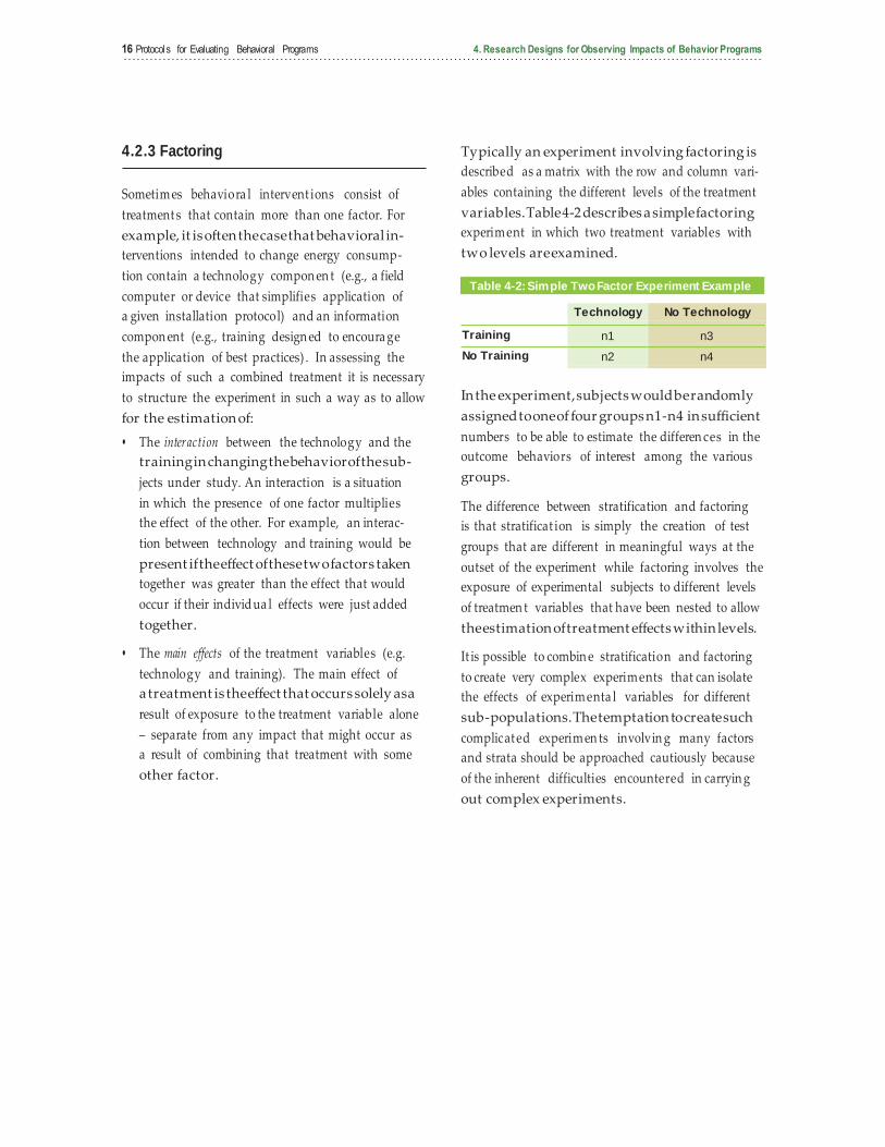
4.2.3 Factoring
Sometim es behaviora l intervent ions consist of
treatment s that contain more than one factor. For
example, it is often the case that behavioral in-
terventions intended to change energy consump-
tion contain a technology compon en t (e.g., a field
computer or device that simplifies application of
a given installation protocol) and an information
compon ent (e.g., training design ed to encoura ge
the application of best practices) . In assessing the
impacts of such a combined treatment it is necessary
to structure the experiment in such a way as to allow
for the estimation of:
• The interaction between the technology and the
training in changing the behavior of the sub-
jects under study. An interaction is a situation
in which the presence of one factor multiplies
the effect of the other. For example, an interac-
tion between technology and training would be
present if the effect of these two factors taken
together was greater than the effect that would
occur if their individ ua l effects were just added
together.
• The main effects of the treatment variables (e.g.
technology and training). The main effect of
a treatment is the effect that occurs solely as a
result of exposure to the treatment variable alone
– separate from any impact that might occur as
a result of combining that treatment with some
other factor.
Typically an experiment involving factoring is
described as a matrix with the row and column vari-
ables containing the different levels of the treatment
variables. Table 4-2 describes a simple factoring
experim ent in which two treatment variables with
two levels are examined.
Technology No Technology
Training n1 n3
No Training n2 n4
In the experiment, subjects would be randomly
assigned to one of four groups n1-n4 in sufficient
numbers to be able to estimate the differen ces in the
outcome behaviors of interest among the various
groups.
The difference between stratification and factoring
is that stratificat ion is simply the creation of test
groups that are different in meaningful ways at the
outset of the experiment while factoring involves the
exposure of experimental subjects to different levels
of treatmen t variables that have been nested to allow
the estimation of treatment effects within levels.
It is possible to combin e stratification and factoring
to create very complex experim ents that can isolate
the effects of experim enta l variables for different
sub-populations. The temptation to create such
complicat ed experim en ts involvin g many factors
and strata should be approached cautiously because
of the inherent difficulties encountered in carryin g
out complex experiments.
Table 4-2: Simple Two Factor Experiment Example
4.2.4 Replication
Perhaps the single most importa nt tool for evalu-
ating the impacts of behavioral interventions is
replication. Replication is said to occur when the
condition s involved in an experim ent are repeated
in order to confirm that a result which has been
report ed can be repeated by a different investigator,
in a different setting, at a different time and under
differen t circumsta nces. If the report ed effect can
indeed be repeated there is reason to be confident
that the reported result is robust and did not arise
by accident or because of something the investigator
did that was not report ed in the results of the study.
While replication is seldom described as something
individual investigators should consider in design-
ing evaluation s it is a very powerf u l tool that should
be used to assess the veracit y of research findings at
the progra m level; and in evaluation s of behaviora l
interventions, investigators should be encouraged
to structure their studies in such s way as to pro-
duce replicat ion s. It is particula rly useful in situ-
ations where multiple experim ent s can be carried
out in different geogra ph ical locations (e.g., among
the various Local Distribut ion Companies (LDCs)
implementing programs) sequentially or simultane-
ously. Evaluators carryin g out behavioral experi -
ments across multiple LDCs should be encoura ged
to design their experiments as replications of a
single administration.
4.3 True Experiments
True experim ents are research designs in which the
evaluator has control over the exposure of experi-
mental subjects to treatments. There are three kinds
of true experim ents – Random iz ed Controlled Trials
(RCT), Randomized Encouragement Designs (RED)
and Regression Discontinuity Designs (RDD). These
research designs provid e the most robust tests of the
impacts of behaviora l interven tions on energy use
related behavior. They are discussed below.
4.3.1 Randomized Controlled Trials (RCT)
The RCT is an evaluation research design in which
experim enta l subjects are randomly assigned to
treatment and control groups; and the results
observed for the groups are compared to discover
whether the treatment has caused a change in
behavior. The process of random assignment causes
the resultin g groups to be statistically identica l on
all characteris tics prior to exposu re to the treatmen t
to within a knowable level of statistical confiden ce
given the sample sizes being employed. This is true
because each and every observation being assigned
to both groups has the same probabilit y of being as-
signed to each group (i.e. 1/n; where n is the number
of total subjects being assigned.) The mathematica l
consequ ence of this assignm ent constraint is that the
treatment and control groups will be more or less
statistically identical after the assignment process
is complet e. That is, the groups will contain about
the same percenta ge of males and females, have the
same average age, come from the same geographical
locations, have about the same amount of prior years
of experience – and so on and so on and so on for
virtually all the variables one can imagine – whether
we can observe these variables or not.
Of course, because samplin g is involved, the above
statement is true to the extent that relatively large
samples are involved and even then only to within
a certain level of statistical confidence. Indeed, any-
thing can happen in the real world – which means
that even with truly random assignmen t with large
samples it is possible to create treatment and control
groups that are not statistically identical. So it is
good practice to check to make sure the groups that
will be studied in an RCT are indeed more or less
identical at least on the outcom e variable before they
are administ ered the treatment. It is also advisable
to obtain and include pre-test measurem ent for both
the treatment and control groups on the outcome
measures of interest to control for any pre-treat m ent
differen ces that may occur on the outcome variable
of interest.

RCT designs are often referred to as the “gold stan-
dard” of research designs to be applied to observ-
ing behavior change. Severa l reasons underlie this
designation. They are:
• Validity – an RCT controls for most of the above
described threats to internal validity – most im-
portantly for selection bias or the possibility that
the groups under study were somehow different
before the experim enta l factor was presented.
• Simplic ity – analyses of results obtained from RCT
designs are simple and straightf orwa rd and do
not rely heavily on assumption s about specifica-
tion of estimation equations or error structures .
They are often as simple as a differen ce in differ-
ences calculation. Consequ ent ly, the estimated
impacts derived from studies employing RCTs do
not depend heavily on the skill or artfulness of
the analyst.
• Repeatability – because these designs are relatively
simple, it is possible to accurately recreate the
conditions under which observations were taken
thereby making replication easy.
Despite these obviou s advantages, there are sev-
eral aspects of RCT designs that require caution
in application. First, the assignm ent of subjects to
experimental treatments does not guarantee that the
groups that are eventually observed in an experi-
ment are equivalent. There are two easy ways in
which the initial random assignment may be invali-
dated during the course of an experim ent. They are:
• Volun teer Bias – randomly assignin g subjects to
treatment and control groups in which treatment
group members must agree to participat e after
assignment can result in treatment and control
groups that are very different . This is the essence
of selection, so care must be taken to ensure that
significan t numbers of randomly assigned sub-
jects do not migrat e out of the study between the
time they are randomly assigned and the time the
results of the treatmen t are observed. If subjects
must volunteer for the treatment or acquiesce
to it, then random assignment to treatment and
control groups should occur after they have vol-
unteered or agreed to be in the study.
• Rejectio n – human subjects virtually always have
the right to withdra w from a treatment to which
they have been experim enta lly assigned. They
may withdra w for reasons that are unrelated to
the experim ent al treatment or they may with-
draw because of the treatment. In either case,
outmigrat ion from the treatment and control
groups may invalidate the effect of the initial
random assignm ent and care must be taken to
ensure that observations for out-migrant s are
properly handled. If the number of customers
who reject the treatment becomes large (i.e.,
more than 1 or 2 percentage points) then it is
necessary to analyzed the results of the experi-
ment as though it was a RED design.
When regulatory policies or concern about cus-
tomer experien ce prohibit the arbitra ry assignm ent
of subjects to experim ent al condition s, it may still be
possible to randomly assign customers to treatment
condition s by using one of the followin g research
tactics:
• Recruit and deny – experimental subjects are
recruited to an experiment with the understand-
ing that participation is not guaranteed (e.g.,
is contingent on winning a lottery). In such a
situation, subjects are told that the experim enta l
treatment is in limited supply and that they will
be placed in a lottery to decide whether they will
receive it. The lottery winners are chosen at ran-
dom and winners are admitted to the treatment
group while losers are assigned to the control
group. Losers may be offered a consolation prize
to reduce their disappointment in not being
chosen for the lottery. As long as the transaction
cost involved in participat in g the lottery are not
too high, this strategy can overcom e objections
that stakehold ers may have to randomly assign-
ing subjects to test conditions. This approach
is particularly useful when the experimental
treatment (e.g., an attractive new technology) is
in limited supply so that it can be argued that the
fairest way to distribut e the benefit is to distribut e
it randomly to interested parties.

• Recruit and delay – like the recruit and deny
design experim enta l subjects are recruit ed to an
experiment with the understanding that partici-
pation in the first year is contingent on winning
a lottery. The lottery winners are chosen at
random and winners are admitted to the treat-
ment group in the first year. Losers are assigned
to a control group which is scheduled to receive
the treatment in the second year. This approach
can be implemented without causing significant
customers dissatisfaction. However, because the
control group must also receive the treatment in
the second year, it will result in higher cost for
equipment and support than the recruit and deny
approach.
4.3.2 RandomizedEncoura
gement Designs (RED)
Sometim es regulat ory or administrat ive consider-
ations require that all subjects who are eligible to
receive some behavioral intervention must receive it
if they desire it. For example, administrat ive policy
might dictate that all qualified HVAC technicians
have access to training that would result in their
receivin g a certificat e that can provid e competit ive
advantage or may be required to provid e certain
contractin g services. In such a situation it is virtu-
ally impossible to deny some contractors access to
the supposed behaviora l intervent ion to create a
legitimate control group.
It is possible to create a legitimate randomized
experim ent when all parties in the market must be
eligible for treatmen t by employin g what is known
as a Random iz ed Encoura gem ent Design (RED).
In a RED design the treatment (e.g., training) is
made available to everyon e who request s it. How-
ever, while all contractors are eligible for training, a
subset of the eligible contract ors is randomly chosen
to receive significantly more encouragement for
seekin g the training than the control group, (which
is not encouraged). If the demand for the training
is relatively low (in the absence of encouragement)
it may be possible to significantly increase the rate
of exposure to the training among volunteers in the
encouraged group by more intensively marketing
the training program to them. The encouragem ent
might include: more intensive efforts to contact and
recruit contractors; providing economic incentives for
participation; or reducing transaction costs associated
with subscribing to the treatment.
The impact of the treatment is estimated by compar-
ing the outcome variable of interest for the random-
ly selected encouraged group with the same out-
come variable for the random ly selected group that
was not encoura ged. This comparis on is referred to
as an intention to treat analysis, as it focuses on mea-
surement of the difference in the behavior between
those who were intended to be treated and those
who were not intended to be treated. Because en-
couragement was randomly assigned, any difference
between the encoura ged and not encoura ged group
must necessarily have resulted from the fact that
the encoura ged group contains more parties who
received the treatment. Because we know the accep-
tance rate in the encoura ged group, it is possible to
inflate the observe difference between the outcome
of interest in the encoura ged and not encoura ged
group to obtain a reliable estimate of the average
impact of the treatment on those who received it.
The analysis of the impact of the encouragement
and treatment is straightf orwa rd algebra and the
results are easily explained. So, one is tempted to
conclud e that the RED design is a “silver bullet” for
overcom in g the difficult ies that are often cited with
the application of RCT designs in evaluations related
to energy use behavior. Unfortunately this is not
the case. As in the case of the RCT design, there are
certain cautions that must be observed when imple-
menting a RED design.

First, the RED design rests on the assumption that
the only factor that is influenced by the encour-
agement applied to the encouraged group is the
acceptance of the treatment . While it is difficult to
imagine circumsta nces in which encoura gem ent to
participat e in a training progra m or receive organi-
zational support would result in other actions that
changed behavior or energy consumption, it is logi-
cally possible that encoura gem en t stimulates some
other actions that either enhance or attenuate the
observed effect of the treatment; and this possibilit y
should be considered in deciding whether to employ
a RED design.
A second and more importan t caution in apply-
ing RED designs arises out of the likely increas e in
sample sizes required to detect effects using a RED
design. In a RED, the measurem ent of the impact of
the treatmen t on behavior is diluted because some
(in many cases most) of the parties who were en-
couraged to be treated did not accept the treatment.
So, it is possible that only a small portion of the
subjects who are encoura ged to be treated actually
accept it. Nevert h eless they are counted as intended
to be treated. The larger the fraction of the group
that was intended to be treated that does not receive
the treatment , the more muted the measurem ent of
the treatment effect will be, and vice versa. So, for
example if 5% of the population normally accepts
the treatmen t without encoura gem ent; and 20% of
the population accepts the treatment with encour-
agement, then it can be said that the encoura gem ent
has significant ly increas ed the rate of acceptance of
the treatment. However, the impact of the treatment
on the outcome measures in the encoura ged group
will be based on the responses of only 20% of sub-
jects who actually received the treatment. So, if the
actual behavior change for individuals receiving the
treatment is 1 unit, then the difference that will exist
between the encoura ged group and the not encour-
aged group will be only 0.2 units. This mathemat ical
fact imposes powerf u l limits on the usefulness of
RED designs. Dependin g on the magnitud e of the
targeted behavior change and the effectiven ess of
encouragement, the RED design may require much
larger sample sizes in treatment groups than the
conventiona l RCT. In cases where the effect of the
treatment on behavior and the acceptance rate for
the treatment are in the single digits, the sample
sizes required to detect the resulting difference
between the behavior in the encoura ged and not
encoura ged groups may be so large as to be practi-
cally impossible to observe.
In most cases, with training progra ms that involve
at most hundreds of subjects, the usefulness of
RED designs will depend heavily on the ability of
evaluators to develop effective encouragement and
even then these designs should be used only when
relatively large impacts on behavior and energy use
are expected.
4.3.3 Regression Discontinuity Designs (RDD)
In the two true experimental designs discussed
above (RCT and RED) subjects are randomly as-
signed to experim enta l groups – thereby establish-
ing their statistical similarity. Under certain circum-
stances, assignm ent of subjects to treatments can
be non-random provid ed subjects are assigned to
treatment and control groups precis ely on the basis
of their score on an interval level variable such as
age, years of experience, number of annual installa-
tions complet ed, etc. Such an experim ent is called
a Regres s ion Discontin uit y Design (RDD). In an
RDD, everyon e above or below some point (the dis-
continuit y) on the selected interva l scale is assigned
to the treatment group, and everyon e else is assigned
to the control group.
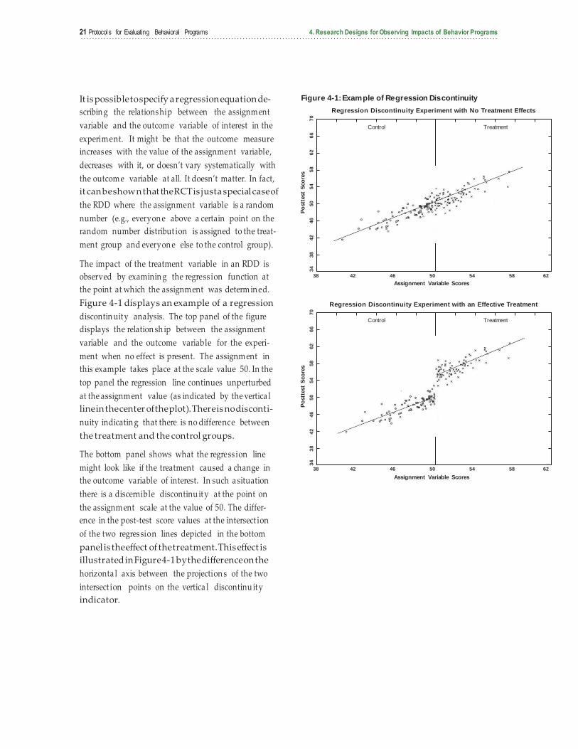
It is possible to specify a regression equation de-
scribin g the relations hip between the assignm ent
variable and the outcom e variable of interest in the
experim ent. It might be that the outcome measure
increas es with the value of the assignment variable,
decreases with it, or doesn’t vary systematically with
the outcom e variable at all. It doesn’t matter. In fact,
it can be shown that the RCT is just a special case of
the RDD where the assignment variable is a random
number (e.g., everyon e above a certain point on the
random number distribut ion is assigned to the treat-
ment group and everyon e else to the control group).
The impact of the treatment variable in an RDD is
observed by examinin g the regress ion function at
the point at which the assignm ent was determ in ed.
Figure 4-1 displays an example of a regression
discontin uit y analysis. The top panel of the figure
displays the relation sh ip between the assignment
variable and the outcome variable for the experi-
ment when no effect is present. The assignm ent in
this example takes place at the scale value 50. In the
top panel the regression line continues unperturbed
at the assignm ent value (as indicated by the vertica l
line in the center of the plot). There is no disconti-
nuity indicatin g that there is no difference between
the treatment and the control groups.
The bottom panel shows what the regress ion line
might look like if the treatment caused a change in
the outcome variable of interest. In such a situation
there is a discernible discontinu it y at the point on
the assignm ent scale at the value of 50. The differ-
ence in the post-test score values at the intersect ion
of the two regres sion lines depicted in the bottom
panel is the effect of the treatment. This effect is
illustrated in Figure 4-1 by the difference on the
horizonta l axis between the projection s of the two
intersect ion points on the vertica l discontinu it y
indicator.
Figure 4-1: Example of Regression Discontinuity
Regression Discontinuity Experiment with No Treatment Effects
38 42 46 50 54 58 62
Assignment Variable Scores
Regression Discontinuity Experiment with an Effective Treatment
38 42 46 50 54 58 62
Assignment Variable Scores
Control Treatment
Control Treatment
Po
stt
est
Sco
res
34
3
8
42
4
6
50
5
4
58
6
2
66
7
0
Po
stt
est
Sco
res
34
3
8
42
4
6
50
5
4
58
6
2
66
7
0
The RDD is an extrem ely powerfu l tool that can be
used when subjects must be assigned to treatment
conditions based on some pre-existing qualification.
It controls all of the possible alternative explanations
for the observed progra m effect. However, there are
certain important caveats that must be met to justify
using this design:
• Assignment to the treatment must be strictly
determined by the assignment variable. Even the
slightest deviation from this requirem ent will
undermine its validity.
• Care must be taken to remove any crossovers
among experiment subjects from the analysis
(i.e., sometim es parties will migrate into the
treatment group from the control group and
vice versa).
• Care must be taken to ensure that the functional
form of the regress ion is correct ly specified. If the
relation sh ip in the estimated regress ion is speci-
fied as linear, but in fact the underlyin g, predicat e
relation sh ip is not, the regres sion discontin uit y
analysis may incorrectly interpret the point of
inflection on the non-linea r function as a discon-
tinuity, resulting in a serious estimation error.
• Likewise, if the treatment interacts with the
assignment variable, so that the slope of the
regression line changes at the assignment variable
due to the treatment effect (causing a jackknife
shaped function), and the function is not proper-
ly specified as such, this will cause a serious error
and one in which the effect of the experimental
treatment will be serious ly underes tim at ed. Pro-
tecting against this possibility requires estimating
non -parametric (nonlinear) regression func-
tions, which imposes an additiona l complexit y.
4.4 Quasi-experiments
It is not always possible to control the assignm ent of
observat ions to treatment and control condition s.
Often, evaluators are given the task of evaluatin g the
impacts of a behavioral program after key marketing
and enrollm en t decisions have been made. It is also
impossible to use true experim ents when treatmen t
condition of interest is compulsory (everyone is
required to be exposed to the treatment), or when
observat ions have the ability to select whether or not
they are subjected to the experimental condition.
These problems commonly occur in experiments
involving training.
When assignment to the treatmen t condition is not
under the control of the experim en t er, the design
of experim ent s is much more complicat ed than it is
with true experim ent s. When observat ion s are ran-
domly assigned to treatment and control conditions
(or assigned on the basis of a pre-exist in g interval
level variable) as is the case with the true experi-
ments all plausible alternative explanations (e.g.,
history, maturation, etc.) for an observed effect are
logically and mathematically eliminated. When this
is not so, it is necessa ry to structure the experim ent/
analysis in such as way to observe whether these
alternative explanations are plausible, measure their
magnitud e, and if possible, control for them analyti-
cally. This is the domain of quasi-experiments.
It should be clear that the decision to abandon ran-
dom assignment can have profound consequences
for the internal validit y of an experim ent al design.
It places a much heavier burden on the research er
to show that the study’s findings are not the result
of some unknown and uncontrolled differen ce be-
tween the treatment and synthesized control groups.
It can be the first step down a slippery slope that
leads to an endless and irresolvable debate about the
veracity of the study’s findings.

There are severa l types of quasi-exp erim enta l de-
signs that are particula rly importa nt in behaviora l
experiments involving training. They vary according
to their robustness (the extent to which they can
achieve the credibilit y of a random experim en t) and
difficulty in their execution. They are:
• Non-equivalent control groups designs
• Interrupted time series designs
• Within subjects designs
4.4.1 Non-equivalent
Control Groups – Matching
In true experim ents, subjects are assigned to treat-
ment and control groups in such a way that they
are either known to be statistically identical prior
to exposure to the treatment factor (as in the case
of the RCT and RED designs) or are different in a
way that is perfectly measured and thus capable of
being statistically controlled. It is not always possible
to implem en t true experim ent s for reasons already
discussed; and for cost and practical reasons it
may be necessary to select control groups after the
subjects to be treated have been selected. These are
called non-equ iva len t control group designs. They
are called non-equivalent control group designs
because the estimates of the impacts of treatment
factors from such designs rests on a comparis on of
treated subjects with subjects who are identified in
such a way that we can never be certain that they are
truly equivalent to the treatment group subjects. The
results obtained from non-equivalent control group
designs are analyzed in exactly the same manner as
they are with true experiments.
The objective of a non-equivalent control group
design is to identify a control group of subjects that
is as similar as possible to the treatmen t group based
on pre-exis tin g informat ion we have about parties
who are eligible for the treatment . Non-equ iva lent
control groups are created by selecting control group
members from the same population (e.g., firms,
business types, markets, regions, cities, trades, etc.)
from which the treatment group came based on
their similarit y to members in the treatment group.
This is done by a process called matching. Match-
ing is a very old idea and dozens of slightly different
matching procedures have been tested over the past
severa l decades. Matching is a highly controversial
proced u re for develop in g control groups because it
is impossible to guarantee that a matching effort (no
matter how sophisticated) has successfully created a
control group that is similar to the treatment group
in all important respects.
Recent profession al practice favors the use of what is
called propens it y score matching – a procedu re that
attempts to match control observat ions with treat-
ment observat ions based on an estimate of the prob-
ability that subjects were selected for (or selected
themselves into) the treatment group. This tech-
nique requires estimation of the probabilit y of selec-
tion into the treatment group using a logit regres-
sion model containin g as many known predict ors of
treatment group participation as can be found.
In simple terms, a logit model is a type of regres sion
model designed to predict the probability that some-
thing happens (e.g., signing up for training) based
on informat ion about readily observa ble indepen -
dent variables that may be correlat ed with selection
into the treated group (e.g., firm size, years of expe-
rience, express ed interest in training, etc.) Once the
paramet ers in the logit model have been estimated,
members of the treatment group and other subjects
who are not part of the treatment group are assigned
propens it y scores based on their characterist ics and
the model parameters. Treatment group subjects
and others are then matched accordin g to the values
of those scores. Once matching has been complet ed,
the results from the treatment and control groups
in the experim ent are analyzed in exactly the same
manner in which the results from true experim ent al
designs are analyzed.

Matching methods by themselves are to be used
with caution because they are prone to the introduc-
tion of bias that cannot be anticipated or measured.
However compellin g the results based on experi-
ence, intuition, or other indicators of a treatment
effect, an experiment involving non-equivalent
control groups does not provid e incontrovert ible
evidence that the observed effect is attributable
solely to the treatment. That said, this may be all that
is possible under some circumstances.
4.4.2 Within Subjects
All of the preced in g experim enta l designs rest on
the comparison of the behavior exhibited by groups
of subjects who have been exposed to treatment
with behavior exhibited by groups that have not
been exposed to a treatment (control groups). The
differen ce between the behaviors exhibit ed by the
two groups (exposed and not exposed ) reflects the
effect of the experimental treatment.
The principa l threat to the validity of such designs
is the possibilit y that the groups were different in
some way that produced the appearance of a treat-
ment effect when one did not really exist. In the true
experim ents, this threat to validity is eliminat ed by
controllin g the assignm ent to treatment and control
groups in such a way as to ensure that the compari-
son groups are statistically identical or different
in ways that are known with certainty. However, it
is not really possible to control for this possibilit y
when non-equivalent control groups are used as the
standard of comparison. That is, it is always possible
that non-equ iva lent control groups are different
from the treatmen t groups in some importan t way
before the onset of the experim enta l treatment . This
problem is inherent in the comparis on of treatment
and control groups to infer the effect of the experi-
mental treatment.
Under some circums tan ce it is possible to avoid this
problem . The solution rests in comparin g what hap-
pens to experim enta l subjects in the presence of and
in the absence of treatment. That is, it rests on ob-
servin g the effect of the treatment (e.g., training) by
comparing the behaviors exhibited by experimental
subjects before the treatment is present ed and after;
or when it is at high levels vs. low levels . In this way,
the subjects in the experiment serve as their own
control group. This experim enta l design is called a
Within Subjects design.
The defining characteristic of a within subjects
design is that each and every experim enta l subject
is exposed to all levels of the experim en ta l factors
under study as well as the absence of the experi-
mental factor (i.e., the control condition). Under
the appropriate conditions this is a very powerfu l
quasi-ex p erim enta l design because it complet ely
eliminat es the possibilit y of selection effects because
it completely eliminates the control group.

4.4.3 Interrupted Time Series
Another quasi-experimental design that is ap-
propriate to studies of the impact of behavioral
intervent ions on energy use related behavior is the
interru pt ed time series design. An interru pt ed time
series design consists of repeat ed measures of the
behavior of interest before and after a treatment has
been administered. This design is particularly useful
when variables related to usage or other frequent ly
measured behaviors are under study – thereby creat-
ing the opportunity to observe the time series of
measurements.
The basic idea behind interrupted time series
designs is that if the onset time of the treatment is
precisely known, it should be possible to observe
and quantify a perturbation in the time trend of the
outcome variable (energy use related behavior) after
the onset of the treatment. In other words, there
should be a measurable change in the functional
relationship between the treatment and the outcome
variable after the treatment is started. In a sense, this
is analogous to regression discontinuity, where time
is the selection indicator. This design depends on
several important considerations:
• The onset time of the treatment can be
definitively established (i.e., it is definitely known
that treatment commenced abruptly at a time
certain).
• The effect of the treatment must be large enough
to rise above the ambient noise level in the
outcome measurem ent (time series data often
contain cycles and random fluctuations that
make it difficult to detect subtle effects of time
trend influences).
• If the treatment is expected to have gradually
impacted the outcome of interest, the time series
before and after the treatment must be long
enough to reflect the change in the intercept or
slope of the outcome variable after the treatment
has occurred.
• The number of observat ions in the series must
be large enough to employ conventional correc-
tions for autocorrelat ion if statistical analysis is
required (as it almost always is).
Like all comparis on s that rest entirely on observin g
the difference in behavior before and after exposure
to treatment the interrupt ed time series designs are
subject to severa l weakn ess es that can undermin e
the validit y of the inference that observed change
has been caused by the experimental treatment.
Most important among these weaknesses is the
possibility that the observed change in the intercept
or slope in the time series may have been caused by
somethin g other than the treatment (i.e., an exog-
enous but contemp oran eous factor with historical
antecedents) . It is also possible that some aspect of
the testing process that is coincid ent with the deliv-
ery of the experim ent al factor is respons ible for the
observed change (e.g., a Hawthorne effect).
To control for such interven in g explanations, a vari-
ety of quasi-ex p erim ent al control techniqu es can be
employed, including: the use of non- equivalent con-
trol groups as described above, adding non-equiv-
alent depend ent variables (i.e., other variables that
are expected to be impacted by the same historical
forces as the dependent variable but not the treat-
ment factor), and manipulatin g the presenta tion of
the treatmen t factor (adding and removin g it) to ob-
serve the impact on the outcom e variable. The latter
is only appropriate when the effect of the treatmen t
factor is expected to be transient. In the parlance of
statistics, these designs are a type of within subjects
or repeated measures design.

Capacity building programs are social interventions designed to lower energy
consumption in residential and commercial buildings by providing training and technical
assistance to various market actors who design, install, operate and service systems
that influence energy consumption in buildings; and by providing expert advice to organi-
zations to assist them in identifying and implementing energy efficiency improvements.
Below are some examples of capacity buildin g
progra ms :
• Resident ial builder training – training and incentives
designed to encourage residential builders to
incorporate energy efficiency and green attributes
into new residential buildings. Program is target-
ed at company executives , designers , marketin g
staff, site superintendents, framers and insulators.
• HVAC installat ion optimizat ion training – training and
incentives to HVAC contractors to encoura ge
them to apply best practices in designing and
installing resident ia l and small commercia l air
conditioning and heat pump installations.
• Energy Manager Training – training for energy man-
agers workin g in large commercial or industria l
organizations.
• Energy Efficiency Service Provider Support Initiat ive –
support to energy service providers and support
organizat ions for deliverin g energy services to
various market segments (e.g., health care, refin-
ing, forestry, mining, etc.). Services will include:
identification of savings opportunities, prepara-
tion of energy managem ent plans, assistance in
identifyin g and promotin g incentive progra m s
and applying for incentives, promot ion of effec-
tive energy management practices, and delivery
of training, outreach and advice regarding
opportunities for energy savings.
While it is self-evident that training key market
participan ts should lead to improvem ent s in the op-
erating efficien cy of critical buildin g systems, there
is a surprising lack of empirical evidence supporting
the proposit ion that such training can encoura ge the
adoption of more efficient technology, ensure that
equipment is properly installed, will cause buildings
to be operated more efficiently or cause significa nt
energy saving measures to be adopted by organi-
zations. This is so because the existing paradigm
for evaluating energy efficiency programs doesn’t
provide for a reasonable means for quantifying the
impacts of these and other efforts to alter energy
consumption by changing behavior.
Training progra ms are, as the name suggests,
genera lly involve classroom training courses
intended to enhance the ability of various actors
in the market to cause reductions in energy
use. The training varies dramatically from
market actor to market actor, but the intended
outcome is the same – reductions in energy
consumpt ion. Segment support progra ms
provid e specializ ed consultin g services to
differen t market segments (e.g., govern m ent and
industries) to assist them in identifyin g
opportun ities for achieving energy savings,
planning, financial assessments, management
presentations and other

services that may enhance the rate at which energy
efficiency investments are achieved. The objective of
these progra m s are to inject expertis e into organiza-
tions to help them overcom e institutiona l and other
hurdles that may impede the adoption of energy
efficien cy projects in complex investm ent environ-
ments. Different evaluation strategies are required
for these two types of programs
To assess the effects of training progra ms on the
market one must:
• Establish the current state of the art and result ing
energy efficiency for the market actions of interest . For
example, in the case of HVAC installation it is
necessary to determine what the typical installa-
tion practices in the market are for establishin g
system sizing, matching coils to air handling
systems and determinin g appropriate air flow
before training is offered. This effort will provide
an understanding of the need for training as
well as the magnitud e of the energy savings that
could result from a progra m design ed to improve
practices . This can be done in a variety of ways.
It is usually done by interviewin g practitioners
to discover the practices they are using. Delphi
groups, focus groups and surveys are used to col-
lect information . In some cases (as in the case of
HVAC contractor training) this work may have
already been done at the time the evaluation is
undertaken. In other cases this may not be the
case and it will need to be undertaken.
• Estimate the effect iveness of the trainin g program in
chang ing the knowledg e, skills and abilit ies of those
exposed to training . This is an empirical study de-
signed to determ in e the effectiven ess of the train-
ing progra m in changing knowled ge, opinions
and practices in the market. For example, in the
case of an HVAC installation training progra m
this might be done by observing installations
that were done before and after training; or by
classroom exercis es and tests intended to test the
knowledge of trainees before and after exposure
to the training.
• Estimate the average improvement in energy efficiency
that results from providin g trainin g to the target market .
For example, in the case of the HVAC installation
contractor training, this could be done by analyz-
ing the difference in estimated energy efficiency
of installation s complet ed by each trainee before
and after exposure to the treatment. This will
produce an estimate of the average uplift in en-
ergy efficien cy (e.g., annual kWh savings, SEER)
that results from exposure to training.
• Assess the persistence of the effect of the trainin g. It is
possible that trainees will cease to use the practices
they learn in training as time passes. Therefore, it
is important to follow up with trainees after signif-
icant time has passed (i.e., 1-2 years) to determin e
how much the effect of the program is decaying.
This may suggest the need for refresher courses or
other actions to resent the effect of the program; or
at a minimum an adjustment will have to be made
in the long term expected savings resulting from
the program.
• Observe any spillover effects that may have occurred
because of training . It is possible (even likely) that
useful practices learned directly in training will
be transferred from trainees to other workers as
time goes on. This should be expected becaus e
skilled workers often use first-hand experien ce
to teach their colleagues useful practices. For
example, in the case of the HVAC installer train-
ing, it might very well be the case that journey-
man HVAC workers who receive the training will
train the apprentices in their companies or even
other apprentices in their trade workin g in differ-
ent companies to apply the techniqu es they learn
in the classroom.

A number of empirica l measurem en ts are required
to address the above issues. Most of the measure-
ments required to evaluate training programs
involve surveys of trainees taken before and after
exposure to training; survey measurements of
parties who do not undergo training (i.e., control
groups); and in some cases survey measurements of
physical facilities (e.g., installed systems affected by
the actions of trainees. In many cases it will be pos-
sible and highly desirable to carry out experim ents
in which the outcom es of market actions taken by
those who have received training (e.g., installations)
are compared with outcomes of market actions
taken by those who have not received training.
Unlike the training initiatives described above the
segment support programs are designed to improve
energy efficiency by provid in g consultin g exper-
tise to specific organizat ions (e.g., municipa lit ies,
schools, hospitals, industries, etc.) to help them
identify cost effective energy efficiency investments
and implement them. The outcome measures of
interest for these initiatives is not a better educated
and more qualified workforce but an accelerat ed
rate of adoption of energy efficient technology by
specific organiza tions. In other words, the effect of
the segment support progra ms is not to improve the
knowledge of the organizations that are being served
by EE specialists, it is to use the efforts of these spe-
cialists to overcom e institution a l barriers that im-
pede adoption of more energy efficient technologies
in organizat ion s. This sort of progra m is particula rly
challengin g to evaluate because very little about the
implem entat ion of the progra m can come under the
control of the evaluator. That is, it is difficult to craft
a true experim ent al design that can be practically
implemented in the context of such a program.
To assess the impact of segment support programs
one must:
• Identify the market segmen ts that should be or
are being targeted (e.g., municipal governments,
state govern m en ts, universit ies and colleges,
school systems, forest products, mining, minera l
extraction, real estate, etc.) and the organiza-
tions inside those segmen ts that have significant
potential for energy efficien cy improvem ent s.
The purpose of this task is to identify the poten-
tial targets of the program. This information is
useful both in directing the work of the energy
efficiency solutions providers and in assessing the
extent which their efforts are being directed at
high value targets for evaluation purposes.
• Estimate the effectiven es s of the service delivery
system in overcom in g barriers to the identifica -
tion and adoption of energy efficient technol-
ogy. This is a very challengin g problem. Energy
savings potential will vary dramatica lly from
sector to sector and within sector from organiza-
tion to organiz ation. Moreover, the service can
only be delivered to organizat ion s that volun -
teer to accept it and it is undoubtedly the case
that organizat ion s that volunteer are inherent ly
more likely to identify and implem ent energy
efficiency improvements than those that do
not. Corresp on d in gly, it will be very difficult to
identify organizat ion s to serve as control groups
for purpos es of identifyin g the effectiven es s of
the progra m. Probably the best way to establish
control groups for the segment support programs
is to divide up the service area geographically and
make segment support available to some areas
and not to others. In this way it would be possible
to compare the rates at which organizations of
different types are implementing energy efficien-
cy improvem ent s for the different geogra ph ica l
locations.

So for example, if there are 50 municipa lities in
one area and 50 in another, and segment sup-
port is only offered in one area and not in the
other, it would be possible to compare the rates
at which the municipa lities in the different areas
are implementing energy efficiency improvement
plans as well as the resultin g savings. Any effort
to quantify the effectiven ess in the absence of the
establishment of such a control group will be sub-
ject to selection effects and therefore will produce
a biased estimate of the effect of the program.
• Estimate the uplift in energy efficiency that
results from provid in g assistance. Plans that are
actually implemented will usually incorporate re-
bates or incentive payments and the calculation s
required to obtain these incentives can be used
to estimate the resulting energy savings. It should
be possible to assess the claimed savings result-
ing from the plans made by organiza tions and if
necessary to verify the accuracy of those claims.
The magnitude of the uplift must be judged in
terms of the increas e in energy savings over and
above the savings that occur in locations where
the segment support progra m s are not offered.
5.1 - Protocol 1:
Define the Situation
The first step in research design is to develop a clear
understanding of the purpose of the evaluation
research and the context in which it is being carried
out. In general, it is expect ed that the evaluator and
project manager for the behavioral intervention will
work collaboratively to answer the questions raised
in this protocol. So, the application of this protocol
is actually a task in which the parties who are car-
rying out and evaluating the training program work
collaboratively to literally define the research design.
Describe the Capacity Building Program:
• Type of Program – Training or Segment
Support
• The target population (i.e., in the case of train-
ing identify market actors that are targeted, in
the case of segmen t support identify the specific
market segments that are being targeted)
• The behavior(s) that is/are targeted for modifica -
tion (e.g., design practices, system specificat ion,
building design, construction practices, installa-
tion, operations, organizat iona l decisions, etc.)
• The mechanis m (s) that is/are expected to change
behavior (e.g. education, feedback, training,
indoctrination, organizational change etc.)
• Whether presentation of the hypothesized behav-
ioral change mechanis m( s) is/are under the con-
trol of the evaluator (i.e., whether the evaluator
can decide which members receive the behavior
change mechanism and which do not)
• The outcomes that will be observed (i.e., adop-
tion of technology, adoption of practices , sales of
efficient technology, energy consumption, rebate
request s, informat ion system access attempts).
The answers to the above questions should be no
more than a page in length each and should describe
the behavioral progra m in sufficient detail to permit
discussion of the experim enta l design alternatives
with stakeholders.
While all of the above question s are important for
identifyin g an appropriate research design for a be-
havioral outcom e evaluation, none are more impor-
tant than question no. 4 – i.e., whether the exposure
to the behavior change mechanis m can be brought
under the evaluator’s control. If the presentat ion of
the treatment can be controlled, then it is possible
to employ true experim ents and reach definitive
conclusions about the effectiveness of the behavioral
mechanis m at relatively low cost. If it is not possible
to control the presentation of the treatment, then
it will be necessary to evaluate the progra m using
quasi-experim ental techniques which are inherently
less reliable than the true experim ent s and rest on
assumptions that may or may not be tenable.

Exposure to the treatmen t may be outside the evalu-
ator’s control for a variet y of reasons. For example,
the progra m may have already been implem ent ed
or be underway when the evaluator is first intro-
duced to the problem . So, the treatment may have
already been present ed to the target audience. It is
also sometim es the case that regulat ors prescribe the
delivery of treatment s – requirin g that all eligible
parties receive a given behaviora l treatment (e.g.,
access to training); and sometim es utility manage-
ment are reluctant to deprive parties who are seek-
ing access to behavioral progra ms – either because
they do not want to disappoint them or because they
want to achieve maximu m effect of the behaviora l
intervent ion. These and other considera tions may
limit the control of the delivery of the experim ent al
treatment of subjects in impact evaluations. The type
of and robustness of the experim enta l design that
can be implem ent ed depend entirely on the extent
of control the evaluator has over the assignment of
subjects to treatments.
Program managers and other stakeholders often re-
sist controllin g the delivery of treatment to custom-
ers. They suspect or know that depriving customers
of treatments they desire can create an unpleasant
customer experien ce that may cause problems for
them and their superiors. So it will often be neces-
sary to educate these parties about the need for
controlled experiments; and to convince them to
accept the highest level of control possible. For this
reason it is appropriate and necessary to plan to
carry out the work required to implem ent Protocol 1
collaboratively with the project manager. The answer
to the question that follows is critical to the eventual
design of the evaluation and will in large measure
govern the usefulness of the study results.
Table 5-1 identifies the level of control you believe
is possible in assigning the treatment to subjects
and why.
Provide a brief discussion of factors that
led you to this conclusion.
This discussion should not exceed five pages and
should carefully state your reasons for concluding
that your level of control is as indicated in section
5.1.4. The purpos e of this element of the protocol
is to demonstrate that the evaluation team has
carefully analyzed the design of the progra m in an
effort to identify opportunities to create randomized
experim enta l groups and has reached their deci-
sion on the level of control based on a good faith
effort to attempt to achieve maximu m control over
the assignm ent of subjects to treatment and control
groups and that you and your client understand
the consequ en ces of the level of control you have
identified.
Table 5-1: Appropriate Experimental Designs Based on Ability to Control
Ability to Control Appropriate Experimental Design
Able to randomize presentation of treatment – mandatory
assignment of subjects to treatment and control conditions
Randomized Controlled Trial (RCT)
Able to deny treatment to volunteers – mandatory assignment
of volunteers to treatment and control conditions
RCT using recruit and deny tactic
Able to delay treatment to volunteers – mandatory assignment
of volunteers to treatment and control conditions
RCT using recruit and delay tactic
Able to randomly encourage subjects to
accept treatment
Randomized Encouragement Design (RED)
Able to assign subjects to treatment based on qualifying
interval measurement (e.g., income, usage, building size, etc.)
Regression Discontinuity Design (RDD)
Unable to assign subjects to treatments Quasi-experimental designs

5.2 - Protocol 2:
Describe the Outcome Variables to be Observed
Among other things, Protocol 1 (Section 5.1.1)
requires the evaluator to describe the behaviors that
are to be modified by the intervention. Observat ions
of two basic outcom es will be required – behavior
changes and energy savings. Behaviors of inter-
est will vary with the design of the intervent ion.
For example, the training for HVAC contractors is
designed to change several very specific behaviors
carried out by sales and installation technicians –
procedures used to estimate equipment size require-
ments, procedures used to select the size of coils,
proced u res used to establish air flow and severa l
other activities. For other training programs the
behaviors of interest may be different. For segment
support progra m s offering EE solutions, the behav-
iors will be very different – includin g changes in the
behavior of organizat ion s such as adopting energy
efficien cy investm ent plan and operatin g plans and
investm en ts in recom m end ed energy efficien cy
investments.
In Protocol 2, the evaluator is required to explicit ly
describe the measurements that will be used to
observe the behaviors of interest before, during and
after exposure to the intervent ion. There are two
broad categories of measurem ent s that arise in the
context of evaluating behavioral interventions – ob-
servations of behavior or actions taken in respons e
to intervent ion s and observat ion s of the impacts of
the intervention on energy consumption.
Protocol 2 consists of a series of questions that are
designed to produce an exhaustive list of outcomes
that will be measured in the evaluation. As discussed
earlier, this list may evolve iteratively if the initial
evaluation design and the budget required to
assess all of the treatment s and outcom es of interest
exceeds what is available, and therefore not every-
thing of interest may be pursued.
In genera l, this protocol is design ed to identify all
of the different types of physical measurements that
must be taken in order to assess the impacts of the
behavioral intervention. These measurements might
include:
• Measurements from tracking systems recording
the progress of marketing efforts indicating who
received program offers, what channels the offers
were transmitted through, how many offers were
sent, what content they received and if and when
they responded to the offers.
• Records of participation in rebate and other
programs that may identify actions taken by
subjects in response to the program
• Measurem ent s from surveys of consum ers
or other market actors taken before and after
exposure to treatments.
• Measurements from tests given to trainees before
and after exposure to training.
• Measurement of energy consumption before,
during and after treatment for treatment and
control groups

Please describe the behavioral outcomes of interest in the study, the operational definitions that
w ill be used to measure them.
Complet e Table 5-2 in as much detail as possible describin g all of the behaviora l and energy savings outcomes
that are expected to occur as a result of the progra m along with operation al definitions of each outcome.
Table 5-2: Table Caption
Behavioral Outcome Operational Definition
Training Programs
• e.g. HVAC Insta lla ti on Contrac tor
Training Program
• Improved performance in carrying out
best practices in calculating system size
requirements and applying other technical
and non-technical practices involved in
installation.
Behavior Measures
• Comp aris on of actua l work befor e and after trainin g or
treated and control trainees,
• written test of train ee knowled g e befor e and after trainin g,
• comp aris on of knowled ge and opinio n s (as measu red by
test) of trainees and comparison group
Training Programs
• Energ y saving s resultin g from
improved performance from
training
Savings Measures
• Comparison of average SEER of systems installed by
treatment and control groups before and after training
• Estim ated annual, month ly, hour ly energ y savin gs given
average SEER difference
• Estimated difference in peak kW if any by hour
• Other energy consumption measurements
Segment Support Programs
• e.g. EE solutions support
to Municipal Governments
Behavior Measures
• Rate of acceptance of assistance in treatment groups
• Expressed interest in assistance for control groups
• Comparison of rate of adoption of different types of
energy eff iciency solutions (e.g., energy eff iciency plans,
f inancial analysis, management presentations, measures
adopted) for treatment and control groups
Segment Support Programs
• Energ y savin gs resultin g
from solutions
Savings Measures
• Comp aris on of annual energ y cons um p tio n for treatment
and control organizations before and after treatment

5.3 - Protocol 3:
Delineate Sub-segments of Interest
Capacity Building programs are sometimes targeted at multiple audiences (e.g., trades or disciplines in the case
of training programs and market segments in the case of EE solutions segment support programs). If there is a
desire to understand how the program affects different market segments, it is important to recognize these dif-
ferent segments during the design process. Protocol 3 requires the evaluator to identify all of the segments that
are of interest in the study.
Complet e the followin g table in as much detail as possible describin g all of the segments that are of interest
in the evaluat ion. Be careful to limit the segment s to those that can be observed for both the treatment and
control group before subjects are assigned to treatment groups. For example, it is possible to determ in e in ad-
vance of treatment whether a person workin g in a given HVAC contractin g firm is a sales agent or an installer.
This might be a useful segment ation variable, as there is some eviden ce that these two disciplin es approach the
installation of new equip m ent differently. It is also importa nt to limit the number of segment s so that 30-100
observations can be taken within each segment and treatment level.
Please describe all of the segments that are of interest in the study.
In Table 5-3, please use one line for each segment of interest.
Table 5-3: Segments of Interest
Segments of Interest
Training Programs
(e.g., different jobs, different sized organizations, different business types, etc.)
Segment Support Programs
(e.g., different types of organizations (municipal governments, school systems, state government
departments), different industries (forest products, light manufacturing, etc.)

5.4- Protocol 4:
Define the Research Design
Protocol 4 is designed to guide the experim enta l design process by asking evaluat ors to answer key questions
designed to identify the theoretica lly correct design, as well as the practical realities that confront real-world
social experim ent ation. When complet in g these question s, it may be useful to refer to Section 5 of this docu-
ment as a guide to selectin g the experim ent al design that best supports the treatments, objectives , and practical
realities associated with the specific experiment under consideration.
Please answer the following questions.
Please use Table 5-4 to complete your answers.
Table 5-4: Questions on Behavior Measures
Question
Behavior
Measures
Energy Consumption
Measures
Will pre-treatment data be available?
Does the appropriate data already exist on all
subjec ts, or do measu rem en ts need to taken in
order to gather pre-treatment data?
How long of a pre-tr eatm ent period of data collec tion
is required?
Is a control group (or groups) required for the
experiment?
Is it possible to randomly assign observations
to treatment and control groups?
Using the framework outlined in Chapter 4, describe the evaluation research des ign that
w ill be used during the evaluation.
This description should explain what type of research design will be used (e.g., RCT, RED, Regres sion Discon-
tinuity, Non-Equ ivalent Control Groups, Within Subjects, etc.) It should describe the treatmen t groups and
control groups and any segment ation (e.g., by trade or industry group) that is contemp lat ed. In the case of true
experim ents, the design should be present ed in a table of the kind present ed in Section 5.2.2 where treatment s
are described on the column headings and segmen ts are described on the rows. If random assignment is either
inapprop riat e or impossible to achieve, the descript ion should explicit ly discuss how suitable comparis on
groups will be identified or how the design otherwis e provid es a comparis on that allows an assessm ent of the
impact of the treatment on behavior and energy consumption.

5.5 - Protocol 5:
Define the Sampling Plan
Once the appropriate experim enta l design has been
selected, a sample plan must be develop ed. Obvi-
ously, experim enta l design and sampling go hand in
hand. While an in depth discussion of sample design
would lead us far afield of the focus of research
design, there are certain critical issues that have to
be address ed in any sample design used to study the
impacts of behavioral interventions. They are:
• Are the results of the research intended to be
extrapolated beyond the experimental setting to
a broader population (e.g., all parties involved in
the installation of HVAC systems in the region
served by IESO)?
• Are there sub-popu lat ion s (strata) for which
precise measurements are required (e.g., sales
agents and installation technicians)?
• What is the absolute minimum level of change
in the depend ent variable( s) that is meaningfu l
from a planning perspective (e.g., 1.5 SEER point
improvem ent in performan ce of installed HVAC
systems)?
• How much sampling error is permissible
(e.g., + or - .1 SEER point)?
• How much statistical confidence is required for
planning purposes (e.g., 90%)?
• Are pre-treatment data available concerning
outcome variable(s) of interest?
The answers to the above questions will greatly
influence the design of the samples to be used in the
study. They cannot and should not be answered by
the sampling statistician. The answers to these ques-
tions must be informed by the policy considerat ions .
They have to be made by the people who will use
the information to make decisions given the results.
Once these requirem ents have been develop ed, a
sampling expert can then determine the sample
composition and sizes needed to meet the
requirements.
Defining the Target Customer Population
Often it will not be necessary to extrapolate the
results of the experim ent to a larger population of
interest. That is, it may not be necessary to general-
ize the results from a given experimental test of a
training progra m to all possible parties who might
be exposed to it. Instead, the purpos e of the experi-
ment may simply be to observe the effect of the
treatment on the population of parties who were ex-
posed to it. In this case it is not necessary to sample
observat ions from the entire population of possible
participants.
However, if the results of the experim ent are to
be statistically extrapolat ed to a larger popula-
tion outside the experim en t, then it is necessary to
draw a repres ent ativ e (i.e., random) sample from
the available population, and the sample has to be
structured so that it is possible to calculate meaning-
ful estimates of the population level impacts using
appropriate sampling weights. To calculate weights
for purposes of extrapolat ion, it is necessary to have
a list of the members of the population of interest,
to sample randomly from that list before assignin g
customers to treatment and control condition s, and
to carefully observe any selection effects that might
emerge in the sampling process so that the extrapo-
lation can be adjusted to take account of them.
If precise measurements are needed for specific sub-
populations (e.g., certain trades or organizat ions
in different industries), then it may be necessary to
over-sample these customers to ensure that enough
observations are present in relevant cells to pre-
cisely estimate the impacts of the treatment. These
are called samplin g strata or blocks as described in
Section 3.

Precision of the Estimates
A critical requirem ent in developing a sample design
for any sort of experim ent is a clear understa nd in g
of the minimu m threshold of difference (between
treated and not treated customers) that is consid-
ered meaningful from the point of view of those
who will be using the results in progra m planning.
As discussed below, the size of the difference that
will be considered to be meaningfu l has profoun d
implications for the required sample size. In general,
the smaller the difference that must be detected,
the larger the sample size (of treatment and control
group customers) needed to detect it. If the cost of
the program is known or can be estimated, it is pos-
sible to identify the minimum change in energy use
that would be required to justify investm ent in it.
For example, suppose a 5% reduction in energy use
would be required to justify investm en t in a given
training program in order for the benefits to out-
weigh the costs. The sample sizes for treatment and
control condition s should be set so that a difference
of at least 5% can be reliably detected 80-95% of the
time. A related issue that also influences the sizes of
samples required in an experim ent is the quantity
of sampling error that is tolerable from the point of
view of planning.
In analyzin g the results obtained from a statisti-
cal experim ent, it is possible to make two kinds of
inferent ia l errors arising from the fact that one is
observin g samples. One can incorrectly conclud e
that there is a differen ce between the treatmen t and
control groups when there isn’t one (because of
sampling variation). This is called a Type I error. Or
one can incorrect ly conclud e that there isn’t a differ-
ence when in fact there is one. This is called at Type
II error. The challenge in designin g experim enta l
samples is to minimiz e both types of errors. This is
done by choosin g sample sizes that minimiz e the
likelihood of these errors.
Type I – Statistical Significance
or Confidence
It is possible to calculate the likelih ood of commit-
ting a Type I error from informat ion concern in g the
inherent variation in the population of interest (the
variance), the required statistical precision (as de-
scribed above), and the sample size. This probability
– called alpha – is generally described as the level
of statistical significa nce or confiden ce. It is often
set to 5% so that the sample size for the experim ent
is such that there is no more than 5% chance (one
chance in 20) of incorrect ly concludin g that there
is a differen ce between the treatment and control
group of a given magnitu d e, when there really isn’t
one. However, as in the case of statistical precision ,
the selection of alpha is subjective; it depends on the
experim ent er’s taste for risk. It could be set to 1% or
10% or any other level with attendant consequ en ces
for confidence in the results. For training and
segment support studies, it should probably be set
to 5%.

Type II – Statistical Power
Type II error is the converse of Type I error –
concluding that the treatment made no difference
when in fact it did. For a given population variance,
specified level of statistical precision and sample size,
the probabilit y of incorrectly concluding that there
isn’t a difference when indeed there is a difference is
determ in ed by the choice of alpha (the probabilit y
of making a Type I error). All other things equal, the
lower the probability of making a Type I error, the
higher the probability of making a Type II error. In
other words, for a given sample size, the more sure
we want to be that we are not incorrectly finding a
statistically significant difference, the less sure we can
be that we have missed a statistically significant differ-
ence. The likelihood of making a Type II error can
be calculated for a given experim ent and generally
decreases as sample size increases. The likelihood of
avoiding a Type II error is generally referred to as the
Please answer the following questions
pertaining to sample planning:
1. Are the measurements from the experiment to
be extrapolated to a broader population?
a. If yes, indicate whether the sample will be
stratified and what variables will be used in the
stratification.
b. If no, describe the list of parties from which the
sampling will be obtained.
2. Are precise measurements required
for sub-populations of interest?
a. If yes, describe the sub-populations for which
precise measurements are desired.
3. What is the minimum threshold of difference
that must be detected by the experiment?
4. What is the acceptable amount of sampling error
or statistical precision and acceptable level of
statistical confidence (i.e., 90%, 95%, 99%)?
statistical power of the sample design. The statisti- cal power used in calculating required sample sizes
for experiments is subjective and, in modern times,
has generally been set at about 90%. That is, it is set
so that only one time in ten will the experimenter
incorrectly conclude that there isn’t a difference of a
specified magnitude when indeed there is one. For
Capacity Building experim ents, statistical power
should probably be set at 90%.
The analysis approach used to estimate impacts can
also have a significant impact on sample sizes. For
example, sampling can be much more statistically
efficient if the effect(s) of the treatment(s) are being
measured as differences (e.g., pre-test, post-test) of
ratios or as regression estimators. This is true because
the variance of these parameters in populations under
study is usually quite a bit smaller than the variance
of the raw variables, and the smaller the inherent
variance of the measurements of interest, the smaller
the required sample size. As discussed below, panel
regression methods with pre-test, post-test experi-
mental designs can significantly reduce sample sizes.
5. Will participants be randomly assigned to
treatment and control conditions or varying
levels of factors under study?
a. If yes, do you expect subjects to select
themselves into the treatment condition?
b. If so, how will you correct for this selection
process in the analysis and sample weighting?
6. If subjects w ill not be randomly assigned to
treatment and control conditions or varying
levels of factors under study:
a. Describe the process that will be used to select
customers for the treatment group(s).
b. Describe the process that will be used to select
customers for the control group, and explain
why this is the best available alternative for cre-
ating a non-equivalent control group.
7. If no control group is used, explain how the
change in the outcome variables of interest will
be calculated.
Please indicate the proposed sample sizes
(w ithin the treatment cells) for the study.
If experim ent s are contemp la t ed (true or quasi-
experiments) please use the table format provided
in 4.2.2 to describe the distribution of sample
across treatment cells and strata.

5.6- Protocol 6:
Identify the Program Recruitment Strategy
Most capacity buildin g progra ms will require outreach to the communit y of eligible participant s to recruit
them to participat e in training or support progra m s. At a minimu m, the evaluation must carefully describe the
recruiting process used to attract program participants.
Please answer the following questions in Table 5-5 regarding the recruiting process and its outcome.
Table 5-5: Questions on Recruiting Process and Outcome
Question Answer
Describe the eligibility criteria
for the program
e.g., partic ipants must be actively employed HVAC sales
or insta lla tio n technic ian s with more than 5 years of experien c e
in the industry
What is the estimated numb er of eligib le
parties in the region under study e.g., 10,000 total (sub-groups unknown)
How were partici pan ts recrui ted to the
program e.g., flyers were mailed to all curren tly licen sed HVAC
contractors in the region
Were partici pan ts random ly assig n ed
to treatment and control conditions
e.g., yes, because of limited availability ½ of interested
parties were random ly admit ted into the prog ram in the first
year and the reminder was asked to wait for training until
the following year
If there were samplin g stra ta indic ate
the number of participants recruited
into each strata and group
e.g. 100 sales technicians in treatment, 100 HVAC installers
in treatment, 100 sales technicians in control and 100 HVAC
technicians in control
It is sometim es the case that multiple recruit in g process es are being tested during the evaluation progra m and
that one of the objectives of the evaluation is to evaluat e recruit m ent strategy alternatives and identify the most
cost-effective approach for purposes of program design, taking into consideration both the number of enrollees
as well as the average savings per customer.
If different recruiting strategies are being tested as part of the program please answer the following questions:
• Describe each of the recruiting options that are being tested in the program including how potential par-
ticipants are being identified, how they are being contacted, what they being told, whether they are being
offered incentives and any other pertinent information.
• Describe the research design that is being used to assess the effectiven es s of alternative recru itin g strategies
includin g: the type of experim ent al design being employed (e.g., RCT, RED), how customers are sampled for
the recruitment and how many potential participants are being selected for each recruiting test.
• Describe how the results of the recruiting strategy tests will be analyzed statistically.

5.7- Protocol 7:
Identify the Length of the Study
In evaluatin g a behaviora l intervent ion it is impor-
tant to understand the expected time required to
carry out the various aspects of the intervent ion, the
expected onset time for the effect of the treatment
and its expected persistence after initial treatment.
These considerat ions will determin e the length of
time that is required to assess the impact of the
treatment and thereby determ in e the length of time
for which the situation must be observed.
Please answer the following questions
pertaining to the experimental time frame.
1. Is it possible to observe the impacts of the treat-
ment for at least two years?
2. If no, how will the persistence of the effect be
determined?
3. Do pre-treatment data for the relevant variables
already exist or must time be allowed to obtain
pre-treatment data?
4. If pre-treat m ent data do not already exist, how
long must the pre-treat m ent period be to support
the experimental objectives?
5. If pre-treatment data do not already exist, can
the experiment be conducted using only post-
treatment data, and what adjustments to sample
design will be required to employ a post-test-only
design?
6. What is the expected amount of time required for
subjects to receive and understan d the informa-
tion being provided to them?
7. What is the expected amount of time needed
by subjects to implement behavioral changes in
response to the information provided?
8. What is the minimu m amount of time the
effect of the treatment must persist to
cost-justify investment on the part of the utility?
9. If the duration of the experim ent is shorter than
the expected persisten ce of the treatment how
will the determination be made as to whether
the effect of the feedback persists long enough to
be cost effective?
10. How much time is needed between when the
research plan is completed and approved, and
when treatments are in place for experimental
participants?
11. How much time is required between when the
final data are obtained from the experim ent al
observations and when the analysis can be
completed?

5.8 - Protocol 8:
Identify Data Requirements and Collection Methods
Please complete the following table identifying the data requirements and data collection methods for each data
elemen t required in the evaluation. The table describes three types of data – energy consumption data, data
describing the behaviors in question and other data.
Table 5-6 should be completed for as many measurements that will be taken during the course of the study.
For example, if the SEER of an installed AC unit is to be collected as part of the evaluation then it should be
described under energy consumption. The description of the variable should include a definition of the variable
in sufficient detail as to permit third parties to understan d what the measurem ent is. It should describe the
frequen cy with which the measurem ent will be taken. For electric it y consumption, the variable might be once
or twice (as in the case of SEER measurements), or it might be monthly, hourly or even momentarily in the
case of electric it y consumpt ion or demand. The method of measurem ent should describe how the data will be
collect ed in as much detail as is required to explain the data collect ion process. If utility billing data will be used
it is sufficient to describe the source and the intervals at which the data will be collect ed. If end-use meterin g
or other measurement procedures are employed, then the technology as well as installation and data collection
protocols should be described.
Table 5-6: Measurements Taken During the Study
Energy Consumption
Description of Variable
Frequency of measurement
Method of Measurement
Issues and Solutions
Behaviors of Interest
Description of Variable
Frequency of measurement
Method of Measurement
Issues and Solutions
Other Data
Description of Variable
Frequency of measurement
Method of Measurement
Issues and Solutions
Behavior data is information describin g the impact of the progra m on target behaviors. Examples of behavior
data that might be appropriat e for training progra ms include: classroom tests of knowled ge, skills or abilities
before and after training, observat ion s of actions taken by trainees before and after training (e.g., installa-
tions or operating condition). Behavior data for segment support might include interviews with organization
members concerning the impacts of the segment support program offerings on the operations of the target and
control organization.
Other data includes all kinds of other data that might be useful in evaluatin g the impacts of the training or
segment support programs including: weather data, data describing the response of the market to the program
offerin g and market data describin g the conditions in the market before, during and after the behavioral inter-
vention has taken place.

In recent years significant efforts have been undertaken to develop and test different
information feedback strategies to cause customers to adjust their behavior related to
energy consumption.
A wide variety of techniqu es have been develop ed
or are under develop m ent includin g: normative
comparis ons designed to present consumers with a
comparis on of their household energy use with that
of other households ; in home display devices that
are intended to inform consumers of their energy
consumption in near real time; adaptive thermostats
that are capable analyzing the energy use related
habits of consum ers and adapting household sys-
tems to those habits and so on.
In some cases these interventions have been shown
to be effective. However, what works on one popu-
lation doesn’t necessarily work on another and
variations in the technical design of in home devices
makes it impossible to infer the performa nce of all
devices from tests conducted on one of them. There-
fore, there is the need to carry out robust testing on
feedback techniqu es to determin e whether they are
effective and if so whether the impacts they produce
are justified in light of the costs.
6.1 - Protocol 1:
Define the Situation
The first step in research design is to develop a clear
understanding of the purpose of the evaluation
research and the context in which it is being carried
out. In general, it is expect ed that the evaluator and
project manager for the behavioral intervention will
work collaboratively to answer the questions raised
in this protocol. So, the application of this protocol
is actually a task in which the parties who are carry-
ing out and evaluatin g the feedback progra m work
collaboratively to literally define the research design.
Describe the Feedback Program(s) to be tested:
• Type of Program – Type of feedback (e.g., neighbor
comparison, IHD, HAN, etc.)
• The target population (e.g. households or
businesses – if these target populations have
specific characteris tics that will narrow the
population of interest down from all customers
such as usage thresholds or SIC categories they
should be described in detail)
• The behavior(s) that is/are targeted for modifica -
tion (e.g., thermostat settings, use of lighting,
time of use, websit e access, acceptance of home
energy audits or other services, etc.)
• The mechanism(s) that is/are expected to change
behavior (e.g. normative comparisons, cognitive
dissonance, commitment, etc.)
• Whether presentation of the hypothesized
behaviora l change mechanis m(s ) is/are under
the control of the evaluator (i.e., whether the
evaluator can decide which members receive the
behavior change mechanism and/or when)
• The outcomes that will be observed (i.e., accep-
tance of treatment, energy use related behaviors,
purchasing behavior, energy consumption, tim-
ing of energy consumption).
The answers to the above questions should be no
more than a page in length each and should describe
the behavioral progra m in sufficient detail to permit
discussion of the experim enta l design alternatives
with stakeholders.

While all of the above question s are important for
identifyin g an appropriate research design for a be-
havioral outcom e evaluation, none are more impor-
tant than question no. 4 – i.e., whether the exposure
to the behavior change mechanis m can be brought
under the evaluator’s control. If the presentat ion of
the treatment can be controlled, then it is possible
to employ true experim ents and reach definitive
conclusions about the effectiveness of the behavioral
mechanis m at relatively low cost. If it is not possible
to control the presentation of the treatment, then
it will be necessary to evaluate the progra m using
quasi-experim ental techniques which are inherently
less reliable than the true experim ent s and rest on
assumptions that may or may not be tenable.
Exposure to the treatment may be outside the evalu-
ator’s control for a variet y of reasons. For example,
increasin gly feedback devices such as IHDs, HAN
systems, and Optimizing Thermostats are being sold
over the counter and through the internet directly to
consumers. It is impossible to control who obtains
such devices and therefore impossible to random ly
assign customers to treatment or control groups.
It might be possible to random ly assign encour-
agement to customers, but that would be difficult
to orchestrate. It is also sometimes the case that
regulat ors prescribe the delivery of treatments –
requirin g that all eligible parties receive a given
behavioral treatment (e.g., access to website infor-
mation concerning energy consumption and energy
saving tips); and sometimes utility management are
reluctant to deprive parties who are seekin g access
to behaviora l progra m s – either because they do not
want to disappoint them or because they want to
achieve maximum effect of the behavioral interven-
tion. These and other considerat ions may limit the
control of the delivery of the experimental treat-
ment of subjects in impact evaluations. The type
of and robustness of the experimental design that
can be implemented depend entirely on the extent
of control the evaluator has over the assignment of
subjects to treatments.
Progra m managers and other stakehold ers often re-
sist controllin g the delivery of treatment to custom-
ers. They suspect or know that deprivin g customers
of treatments they desire can create an unpleasant
customer experience that may cause problems for
them and their superiors. So it will often be neces-
sary to educate these parties about the need for
controlled experiments; and to convince them to
accept the highest level of control possible. For this
reason it is appropriate and necessary to plan to
carry out the work required to implem ent Protocol 1
collaboratively with the project manager. The answer
to the question that follows is critical to the eventual
design of the evaluation and will in large measure
govern the usefulness of the study results.
In Table 6-1, identify the level of control you believe is
possible in assigning the treatment to subjects and why.
Table 6-1: Table Caption
Ability to Control Appropriate Experimental Design
Able to randomize presentation of treatment – mandatory
assignment of subjects to treatment and control conditions
Randomized Controlled Trial (RCT)
Able to deny treatment to volunteers – mandatory assignment
of volunteers to treatment and control conditions
RCT using recruit and deny tactic
Able to delay treatment to volunteers – mandatory assignment
of volunteers to treatment and control conditions
RCT using recruit and delay tactic
Able to randomly encourage subjects to accept treatment Randomized Encouragement Design (RED)
Able to assign subjects to treatment based on qualifying interval
measurement (e.g., income, usage, building size, etc.)
Regression Discontinuity Design (RDD)
Unable to assign subjects to treatments Quasi-experimental designs

Provide a brief discussion of factors that
led you to this conclusion.
This discussion should not exceed five pages and
should carefully state your reasons for concluding
that your level of control is as indicated in section
6.1.4. The purpos e of this element of the protocol is
to demonstrate that the evaluation team has carefully
analyzed the design of the program in an effort to
identify opportunities to create randomized experi-
mental groups and has reached their decision on the
level of control based on a good faith effort to attempt
to achieve maximum control over the assignment of
subjects to treatment and control groups and that you
and your client understand the consequences of the
level of control you have identified.
6.2 Protocol 2:
Describe the Outcome Variables to be Observed
Among other things, Protocol 1 (Section 6.1)
requires the evaluator to describe the behaviors that
are to be modified by the intervention. Observat ions
of severa l basic outcom es will be required. These
include:
• The acceptance rate of feedback;
• Changes in appliance acquisition behavior;
• Changes in energy use related behavior; and
• Changes in other behaviors (e.g., knowledge,
opinions and attitudes).
Specific behaviors of interest will vary with the
design of the interven tion. For example, some feed-
back techniques are provided to all customers by
default. This is virtually always the case with written
normative comparis ons . In other cases, customers
may be offered feedba ck technology a zero cost or
reduced cost and make the decision whether or not
to accept it. These two very different deploym ent
strategies require the collection of very different out-
come measures for measuring customer acceptance.
In Protocol 2, the evaluator is required to explic-
itly describe the measurem ents that will be used
to observe the behaviors of interest before, during
and after exposure to the intervent ion. Protocol 2
consists of a series of questions that are designed
to produce an exhaustive list of outcomes that will
be measured in the evaluation. As discussed earlier,
this list may evolve iteratively if the initial evaluation
design and the budget required to assess all of the
treatment s and outcomes of interest exceeds what
is available, and therefore not everything of interest
may be pursued.
In genera l, this protocol is design ed to identify all
of the different types of physical measurements that
must be taken in order to assess the impacts of the
behavioral intervention. These measurements might
include:
• Measurements from tracking systems recording
the progress of marketing efforts indicating who
received program offers, what channels the offers
were transmitted through, how many offers were
sent, what content they received and if and when
they responded to the offers.
• Records of participation in rebate and other pro-
grams that may identify actions taken by subjects
in response to the program
• When enabling devices are used – measurements
of device activation rates and reasons for activa-
tion failure
• Measurements from surveys of consumers or
other market actors taken before and after
exposure to treatments.
• Measurements of drop-out rates and reasons for
departing the program.
• Measurement of energy consumption before,
during and after treatment for treatment and
control groups

Please describe the behavioral outcomes of interest in the study, the operational definitions
that w ill be used to measure them.
Complet e Table 6-2 in as much detail as possible describin g all of the behaviora l and energy savings outcomes
that are expect ed to occur as a result of the progra m along with operation al definitions of each outcom e. The
table shows an example of the level of detail that is required for feedback experim ents involvin g Normat ive
Comparisons and Feedback.
Table 6-2: Behavioral Outcome and Operational Definition
Behavioral Outcome Operational Definition
Normative Comparisons
• Customer acceptance
• Energ y rela ted knowled ge,
skill and opinions
• Appliance acquisition behaviors
• Energy use related behavior.
Behavior Measures
• Customer subscription rate (for opt-in delivery) and opt-out rate
(for default delivery) from tracking system
• Survey s of treatm en t and control custom ers’ knowled g e, skills and
opinions, reported appliance acquisition behavior and reported
energy use related behavior before and after treatment
Normative Comparisons
• Energy savings resulting from
providing normative comparisons
Savings Measures
• Observed differences in monthly or annual energy consumption
and deman d (kWh, therm s) for treatm en t and control group s before
and after treatment from billing systems
Other Feedback Strategies
(i.e., IHD, HAN Optimizing Thermostats)
• Custom er accep tanc e
• Device commis sionin g
• Device utilization
• Energ y rela ted knowled ge,
skill and opinions
• Appliance acquisition behaviors
• Energy use related behavior
• Usability
• Persistence
Behavior Measures
• Customer acceptance rate from tracking system
• Device commissioning rate from MDMS or other tracking system
• Interv iews/focus groups with customer serv ice agents
• Interv iews with customers regarding commissioning problems
• Survey s of treatm ent custom er s regard in g satisfac tio n with
acquisition/installation process
• Survey s of treatm en t custom er s and contro l custom er s’ knowl edg e,
skills and opinions, reported appliance acquisition behavior and
reported energy use related behavior before and after treatment
• Focu s group s with treatm en t custo m ers regard in g usability and
persistence
Other Feedback Strategies
(i.e., IHD, HAN Optimizing Thermostats)
• Energ y saving s resultin g from
providing technology
Savings Measures
• Observed differences in monthly or annual energy consumption
and deman d (kWh, therm s) for treatm en t and control group s before
and after treatment from billing systems
Website
• Customer acceptance
• Website access
• Website utilization
• Opinions about website
• Energ y rela ted knowled ge,
skill and opinions
• Energy use related behavior
• Usability
• Persistence
Behavior Measures
• Website access from tracking system
• Page views from tracki ng system
• Return rate from trackin g system
• Focus groups with customers regarding usability
• Survey s of treatm ent custom er s regard in g satisfac tio n with
website content and performance
• Survey s of treatm en t custom er s and contro l custom er s’ knowl edg e,
skills and opinions, reported appliance acquisition behavior and
reported energy use related behavior before and after treatment

6.3 - Protocol 3:
Delineate Sub-segments of Interest
Feedback programs are sometimes targeted at
multiple audiences (e.g., customers on time vary-
ing rates, disadvantaged customers, customers with
certain heating or cooling devices, etc.). If there is
a desire to understand how the progra m affects dif-
ferent market segments , it is important to recogn iz e
these different segments during the design process.
Protocol 3 requires the evaluat or to identify all of
the segments that are of interest in the study.
Complet e the followin g table in as much detail as
possible describin g all of the segments that are of
interest in the evaluation. Be careful to limit the
segments to those that can be observed for both
the treatment and control group before subjects are
assigned to treatment groups. For example, it is pos-
sible to determ in e in advance of treatment whether
a household is on a rate that qualifies for a discount
6.4 - Protocol 4: Define the Research Design
or if it is on time varying rates. It is not possible to
determine the approximate annual income of the
household. The former are good candidates for strat-
ification, while the later are is not. It is also impor-
tant to limit the number of segments so that 30-100
observat ions can be taken within each segment and
treatment level.
Please describe all of the segments that are of
interest in the study.
Please use one line for each segment of interest in
Table 6-3.
Table 6-3: Segments of Interest
Segments of Interest
IHD, HAN, Optimizing Thermostats,
(e.g., rates, usage categories, assisted
customers, etc.)
Website
(e.g., Current MyAccount customers, engaged
customers, behavioral segments etc.)
Protocol 4 is designed to guide the experim enta l design process by asking evaluat ors to answer key questions
designed to identify the theoretica lly correct design, as well as the practical realities that confront real-world
social experim ent ation. When complet in g these question s, it may be useful to refer to Section 4 of this docu-
ment as a guide to selectin g the experim ent al design that best supports the treatments, objectives , and practical
realities associated with the specific experiment under consideration.
Please answer the following questions.
Please use Table 6-4 to complete your answers.
Table 6-4: Questions on Behavior and Energy Consumption Measures
Question
Behavior
Measures
Energy Consumption
Measures
Will pre-treatment data be available?
Does the appropriate data already exist on all subjects, or do
measu rem ents need to taken in order to gather pre-tr eatm ent data?
How long of a pre-treatment period of data collection is required?
Is a control group (or groups) required for the experiment?
Is it possible to randomly assign observations to treatment and
control groups?
Using the framework outlined in Chapter 4,
describe the evaluation research design that
w ill be used during the evaluation.
This description should explain what type of re-
search design will be used (e.g., RCT, RED, Regres-
sion Discontinuity, Non-Equivalent Control Groups,
Within Subjects, etc.) It should describe the treat-
ment groups and control groups and any segmen ta-
tion (e.g., customer type, usage category, etc.) that is
contemp lat ed. In the case of true experim ent s, the
design should be presented in a table of the kind
presented in Section 4.2.2 where treatments are
described on the column headings and segments
are described on the rows. If random assignment is
either inapprop riat e or impossible to achieve, the
descript ion should explicit ly discuss how suitable
comparis on groups will be identified or how the
design otherwise provides a comparison that allows
an assessment of the impact of the treatment on
behavior and energy consumption.
6.5 - Protocol 5:
Define the Sampling Plan
Once the appropriate experim enta l design has been
selected, a sample plan must be develop ed. Obvi-
ously, experim enta l design and sampling go hand in
hand. While an in depth discussion of sample design
would lead us far afield of the focus of research
design, there are certain critical issues that have to
be address ed in any sample design used to study the
impacts of behavioral interventions. They are:
• Are the results of the research intended to be
extrapolat ed beyond the experim ent al setting to
a broader population (e.g., all households eligible
to receive the technology in the region served by
IESO)?
• Are there sub-popu lat ions (strata) for which
precise measurements are required (e.g., usage
categories or other segments)?
• What is the absolute minimum level of change
in the dependent variable(s) that is meaningful
from a planning perspective (e.g., 5% reduction
in electricity or gas consumption)?
• How much sampling error is permissible
(e.g., + or – 1%)?
• How much statistical confidence is required for
planning purposes (e.g., 90%)?
• Are pre-treatment data available concerning
outcome variable(s) of interest?
The answers to the above questions will greatly
influence the design of the samples to be used in the
study. They cannot and should not be answered by
the sampling statistician. The answers to these ques-
tions must be inform ed by the policy considerat ions .
They have to be made by the people who will use
the information to make decisions given the results.
Once these requirem ents have been develop ed, a
sampling expert can then determine the sample
composition and sizes needed to meet the
requirements.
Defining the Target Customer Population
Often it will not be necessary to extrapolate the
results of the experiment to a larger population of
interest. That is, it may not be necessa ry to generalize
the results from a given experim en ta l test of a tech-
nology to all possible parties who might be exposed
to it. With large scale feedback technologies targeted
at the general market, extrapolation is an important
consideration. However, in testing emergin g technol-
ogies like IHDs, HAN devices and Websites, thoughts
about extrapolation are futile. Virtually anyone who
agrees to participate in a test of a new technolog y is
an early adopter and there is no reason to believe that
impacts of technology on this market segment foretell
how the technology will be taken up in the general
market. So, it is possible that in many cases the pur-
pose of the experiment will simply be to observe the
effect of the treatment on the population of parties
who were exposed to it. In this case it is not necessary
to sample observations from the entire population of
possible participants.

However, if the results of the experim ent are to
be statistically extrapolat ed to a larger popula-
tion outside the experim en t, then it is necessary to
draw a repres ent ativ e (i.e., random) sample from
the available population, and the sample has to be
structured so that it is possible to calculate meaning-
ful estimates of the population level impacts using
appropriate sampling weights. To calculat e weights
for purposes of extrapolat ion, it is necessary to have
a list of the members of the population of interest,
to sample randomly from that list before assignin g
customers to treatment and control condition s, and
to carefully observe any selection effects that might
emerge in the sampling process so that the extrapo-
lation can be adjusted to take account of them.
If precise measurem ent s are needed for specific
sub-populations (e.g., customer types or size cat-
egories) , then it may be necessary to over-sa mp le
these customers to ensure that enough observations
are present in relevant cells to precisely estimate the
impacts of the treatment. These are called sampling
strata or blocks as described in Section 3.
Precision of the Estimates
A critical requirem ent in developing a sample design
for any sort of experim ent is a clear understa nd in g
of the minimu m threshold of difference (between
treated and not treated customers) that is consid-
ered meaningful from the point of view of those
who will be using the results in progra m planning.
As discussed below, the size of the difference that
will be considered to be meaningfu l has profoun d
implications for the required sample size. In general,
the smaller the difference that must be detected,
the larger the sample size (of treatment and control
group customers) needed to detect it. If the cost of
the program is known or can be estimated, it is pos-
sible to identify the minimum change in energy use
that would be required to justify investm ent in it.
For example, suppose a 5% reduction in energy use
would be required to justify investm ent in a given
training progra m in order for the benefits to out-
weigh the costs. The sample sizes for treatment and
control condition s should be set so that a difference
of at least 5% can be reliably detected 80-95% of the
time. A related issue that also influences the sizes of
samples required in an experim ent is the quantity
of sampling error that is tolerable from the point of
view of planning.
In analyzin g the results obtained from a statisti-
cal experim ent, it is possible to make two kinds of
inferent ia l errors arising from the fact that one is
observin g samples. One can incorrectly conclud e
that there is a differen ce between the treatmen t and
control groups when there isn’t one (because of
sampling variation). This is called a Type I error. Or
one can incorrect ly conclud e that there isn’t a differ-
ence when in fact there is one. This is called at Type
II error. The challenge in designin g experim enta l
samples is to minimiz e both types of errors. This is
done by choosin g sample sizes that minimiz e the
likelihood of these errors.
Type I – Statistical Significance or Confidence
It is possible to calculate the likelih ood of commit-
ting a Type I error from informat ion concern in g the
inherent variation in the population of interest (the
variance), the required statistical precision (as de-
scribed above), and the sample size. This probability
– called alpha – is generally described as the level
of statistical significa nce or confiden ce. It is often
set to 5% so that the sample size for the experim ent
is such that there is no more than 5% chance (one
chance in 20) of incorrect ly concludin g that there
is a differen ce between the treatment and control
group of a given magnitu d e, when there really isn’t
one. However, as in the case of statistical precision ,
the selection of alpha is subjective; it depends on the
experim ent er’s taste for risk. It could be set to 1% or
10% or any other level with attendant consequ en ces
for confidence in the results. For training and
segment support studies, it should probably be set
to 5%.

Type II – Statistical Power
Type II error is the converse of Type I error – con-
cluding that the treatment made no difference when
in fact it did. For a given population variance, speci-
fied level of statistical precision and sample size,
the probabilit y of incorrect ly concludin g that there
isn’t a differen ce when indeed there is a difference is
determ in ed by the choice of alpha (the probabilit y
of making a Type I error). All other things equal, the
lower the probability of making a Type I error, the
higher the probabilit y of making a Type II error. In
other words, for a given sample size, the more sure
we want to be that we are not incorrectly finding a
Please answer the following questions pertaining to
sample planning:
1 . Are the measurements from the experiment to be
extrapolated to a broader population?
a. If yes, indicate whether the sample will be strati-
fied and what variables will be used in the stratifi-
cation.
b. If no, describe the list of parties from which the
sampling will be obtained.
2 . Are precise measurements required for sub-
populations of interest?
a. If yes, describe the sub-populations for which precise measurements are desired.
statistically significant difference, the less sure we
can be that we have missed a statistically significant
differen ce. The likelih ood of making a Type II error
can be calculat ed for a given experim ent and gener-
ally decreas es as sample size increases. The likeli-
hood of avoidin g a Type II error is genera lly referred
to as the statistical power of the sample design. The
statistical power used in calculating required sample
sizes for experim ents is subjective and, in modern
times, has genera lly been set at about 90%. That is,
it is set so that only one time in ten will the experi-
menter incorrect ly conclud e that there isn’t a differ-
ence of a specified magnitud e when indeed there is
one. For Capacity Buildin g experim ents, statistical
power should probably be set at 90%.
The analysis approach used to estimate impacts can
also have a significa nt impact on sample sizes. For
example, sampling can be much more statistically
efficient if the effect(s) of the treatment( s) are being
measured as differen ces (e.g., pre-test, post-test)
of ratios or as regression estimators. This is true
because the variance of these paramet ers in popula-
tions under study is usually quite a bit smaller than
the variance of the raw variables, and the smaller the
inherent variance of the measurem en ts of interest,
the smaller the required sample size. As discussed
below, panel regression methods with pre-test, post-
test experim en ta l designs can significan tly reduce
sample sizes.
3 . What is the minimum threshold of difference that
must be detected by the experiment?
4 . What is the acceptable amount of sampling error
or statistical precision and acceptable level of
statistical confidence (i.e., 90%, 95%, 99%)?
5 . Will participants be randomly assigned to treat-
ment and control conditions or varying levels of
factors under study?
a. If yes, do you expect subjects to select themselves
into the treatment condition?
b. If so, how will you correct for this selection
process in the analysis and sample weighting?
6 . If subjects w ill not be randomly assigned to
treatment and control conditions or varying
levels of factors under study:
a. Describe the process that will be used to select
customers for the treatment group(s).
b. Describe the process that will be used to select
customers for the control group, and explain why
this is the best available alternative for creating a
non-equivalent control group.
7 . If no control group is used, explain how the
change in the outcome variables of interest will
be calculated.
Please indicate the proposed sample sizes
(w ithin the treatment cells) for the study.
If experiments are contemplated (true or quasi-
experim ents) please use the table format provid ed
in 4.2.2 to describe the distribu tion of sample across
treatment cells and strata.

6.6 - Protocol 6:
Identify the Program Recruitment Strategy
Sometim es feedback progra m s are operated on an opt-in basis. That is, the treatment is given only to volun-
teers. When this is true, the recruit m ent strategy can affect the outcom e of the evaluation. At a minimu m, the
evaluation must carefully describe the recruiting process used to attract program participants.
Please answer the following questions in Table 6-5 regarding the recruiting process and its outcome.
Table 6-5: Recruiting Process Questions
Question Answer
Describe the eligibility criteria for the program
e.g., househ ol ds in single family dwel ling s located
in climate zones X and Y
What is the estimated numb er of eligib le parties
in the region under study
e.g., 1 million
How were partic ipants recruited to the program e.g., flyers were mailed to all curren tly eligib le hous eho ld s
Were partici pan ts random ly assig n ed to
treatment and control conditions
e.g., yes, because of limited availability ½ of interested
parties were rando m ly admitted into the prog ram in the
first year and the remin d er was asked to wait for trainin g
until the following year
If there were samplin g stra ta indicate the numb er of
participants recruited into each strata and group
e.g. 500 custo m ers were samp led in each of
4 sampling strata
It is sometim es the case that multiple recruit in g process es are being tested during the evaluation progra m and
that one of the objectives of the evaluation is to evaluat e recruit m ent strategy alternatives and identify the most
cost-effective approach for purposes of program design, taking into consideration both the number of enrollees
as well as the average savings per customer.
If different recruiting strategies are being tested as part of the program please answer the following questions:
• Describe each of the recruiting options that are being tested in the program including how potential par-
ticipants are being identified, how they are being contacted, what they being told, whether they are being
offered incentives and any other pertinent information.
• Describe the research design that is being used to assess the effectiven es s of alternative recru itin g strategies
includin g: the type of experim ent al design being employed (e.g., RCT, RED), how customers are sampled for
the recruitment and how many potential participants are being selected for each recruiting test.
• Describe how the results of the recruiting strategy tests will be analyzed statistically.

6.7 - Protocol 7:
Identify the Length of the Study
In evaluatin g a behaviora l intervent ion it is impor-
tant to understand the expected time required to
carry out the various aspects of the intervent ion, the
expected onset time for the effect of the treatment
and its expected persistence after initial treatment.
These considerat ions will determin e the length of
time that is required to assess the impact of the
treatment and thereby determ in e the length of time
for which the situation must be observed.
Please answer the following questions
pertaining to the experimental time frame.
1. Is it possible to observe the impacts of the treat-
ment for at least two years?
2. If no, how will the persistence of the effect be
determined?
3. Do pre-treatment data for the relevant variables
already exist or must time be allowed to obtain
pre-treatment data?
4. If pre-treat m ent data do not already exist, how
long must the pre-treat m ent period be to support
the experimental objectives?
5. If pre-treatment data do not already exist, can
the experiment be conducted using only post-
treatment data, and what adjustments to sample
design will be required to employ a post-test-only
design?
6. What is the expected amount of time required for
subjects to receive and understan d the informa-
tion being provided to them?
7. What is the expected amount of time needed
by subjects to implement behavioral changes in
response to the information provided?
8. What is the minimum amount of time the ef-
fect of the treatmen t must persist to cost-justify
investment on the part of the utility?
9. If the duration of the experim ent is shorter than
the expected persisten ce of the treatment how
will the determination be made as to whether
the effect of the feedback persists long enough to
be cost effective?
10. How much time is needed between when the
research plan is completed and approved, and
when treatments are in place for experimental
participants?
11. How much time is required between when the
final data are obtained from the experim enta l
observat ions and when the analysis can be com-
pleted?

6.8 - Protocol 8:
Identify Data Requirements and Collection Methods
Please complet e Table 6-6 identifyin g the data requirem ents and data collection methods for each data element
required in the evaluation. The table describes three types of data – energy consumption data, data describin g
the behaviors in question and other data.
Table 6-6 should be complet ed for as many measurem ent s that will be taken during the course of the study.
For example, if electric and gas consumpt ion are to be collect ed as part of the evaluat ion then they should
be described in separate entries under energy consumption. The description of the variable should include a
definition of the variable in sufficien t detail as to permit third parties to understan d what the measurem ent
is. It should describe the frequency with which the measurem ent will be taken. For electric it y consumpt ion,
the variable might be monthly, hourly or even momenta rily in the case of electricit y consumption or demand.
The method of measurem ent should describe how the data will be collect ed in as much detail as is required to
explain the data collection process. If utility billing data will be used it is sufficient to describe the source and
the interva ls at which the data will be collect ed. If end-use meterin g or other measurem ent procedu res are
employed, then the technolog y as well as installation and data collect ion protocols should be described.
Table 6-6: Data Requirements
Energy Consumption Description of Variable
Frequency of measurement
Method of Measurement
Issues and Solutions
Behaviors of Interest
Description of Variable
Frequency of measurement
Method of Measurement
Issues and Solutions
Other Data
Description of Variable
Frequency of measurement
Method of Measurement
Issues and Solutions
Behavior data is information describing the impact of the program on target behaviors. Examples of behavior data
that might be appropriate for feedback programs might include: reported recent history of appliance purchases,
an inventory of energy saving actions taken since the start of the behavioral intervent ion, percept ion s and
opinions about energy use, reported conversations among the family or with neighbors about energy consump-
tion, etc..
Other data includes all kinds of other data that might be useful in evaluating the impacts of the feedback
progra ms including: weather data, data describin g the response of the market to the program offering and market
data describing the conditions in the market before, during and after the behaviora l intervention has taken place.

Education and awareness campaigns are designed to change behavior or facilitate
change in behavior by providing information to consumers.
Such campaigns assume that consumers are reason-
ing beings who use informat ion about the conse-
quences of their actions to formulat e and undertake
actions (behaviors ) to achieve desired outcomes.
There are very well developed social science theories
express in g the causal relations hip between percep-
tion, belief, intention and action. That is, there are
well develop ed theories about how opinions are
shaped and how opinions shape behavior. These
theories -- generally referred to under the head-
ing of Reasoned Action Theories -- hold that it is
possible to educate people about the consequ en ces
of their actions, make them aware of the extent to
which their actions are normatively acceptable and
encoura ge them to formulat e intentions to behave in
a manner that is more in line with positive conse-
quences and more normatively acceptable. Through
this causal chain, consumers and other actors in
the energy market are expected to change their
behavior. Of course, the underlyin g social science
theories can be much more complicat ed than this,
but in broad outline terms, they all share these basic
tenants.
Education and awaren es s campaign s have been in
existence in the energy policy arena for at least four
decades. Indeed, the first efforts to systematica lly
change energy use related behavior were primarily
education campaigns. These early efforts focused on
informin g consumers of the availabilit y of energy
efficient technology alternatives, of the econom ic
benefits of energy efficiency and conservat ion, of
the societal consequences of energy consumption
and so on. They were carried out by govern m ent and
utilities under the assumption that once consum ers
knew the facts they would behave appropriat ely.
Education and awareness campaigns can have a
wide variet y of goals. They can be designed to cause
widespread changes in energy consumption. For ex-
ample, in 2001 in Californ ia serious power shortages
created the need for dramatic reductions in elec-
tricity consumpt ion on the part of business es and
households . During that period, the Californ ia state
govern m ent, in partnersh ip with utilities and local
govern m ent s implem ent ed a wide spectru m public
education and awaren ess campaign designed to en-
courage consumers to lower their energy consump-
tion overall – and in particula r on hot summer days.
This campaign consisted of newspap er, televis ion
and radio advertis in g, bill inserts and other special-
ized marketin g collateral designed to explain the
seriousn ess of the situation, inform consumers of
the offer to reduce electric bills by 20% for consum-
ers who lowered their consumption (year on year)
by 20%, and provide them with tips about how to
reduce their energy use.

This Flex Your Power campaign was relatively large
involving about $45 million in paid and earned
advertis in g over a two year period. However, there
are many examples of more modest efforts designed
to accomplish less ambitious goals. For example, in
Californ ia small and mediu m sized commercia l and
industria l firms are being defaulted to time of use
rates between Novem ber of 2012 and Novem ber of
2014. An intensive education/a wa ren ess campaign
is being used to inform customers when they will be
defaulted and of the actions they can take to lower
their costs either by reducin g their energy consump-
tion overall or by restricting their use during the
peak hours in the afternoon. This is a relatively small
and focused education effort that each year involves
educatin g about 150,000 customers, costing only a
few million dollars each year.
Education and awareness campaigns can be
targeted at all levels of society. They can be national
campaign s such as DOE’s Energy Star Progra m,
campaign s carried out by state and local govern-
ments as described above, campaign s focused on
individual organizations or businesses – even cam-
paigns focused on schools and neighborhoods.
One can imagin e a very large number of examples
of education and awaren es s campaigns with differ-
ing goals, messages, target audiences and contact
strategies. However, the critical evaluation questions
that must be answered for virtually all of these
campaigns are the same. Namely,
• What were the beliefs, opinions, attitudes,
intentions and behaviors of the target audience
prior to exposu re to the education or awaren ess
campaign;
• What were the beliefs, opinions, attitudes,
intentions and behaviors of the target audience
after exposu re to the education or awaren ess
campaign; and most importantly
• Did the education campaign cause any
observable change in the beliefs, opinions,
attitudes, intentions and behaviors?
Beyond these basic question s it is possible to address
a number of other interestin g and important ques-
tions in the context of evaluating an education or
awareness campaign. These include:
• What combinations of message, format and
channel were most effective in educating or
informin g importa nt market segments ?
• Did the education campaign have an impact on
targeted customers’ belief that their behavior was
normatively acceptable?
• Did exposure to the education campaign increase
the likelihood that consumers expressed the
intention to engaged in desired energy use related
behavior?
• Did exposure to the education campaign increase
the likelihood that consumers engaged in desired
energy use related behavior?
While the ultimate objective of education and
awaren ess campaigns may be to cause a change
in energy consumpt ion on the part of the target
population by providing education, it is very dif-
ficult to conclusively demonst rat e a causal connec-
tion between attitude change and behavior change.
The causal linkage between education and action is
mitigated through a number of important interven-
ing factors that can significan tly interfere with the
express ion of desired energy use related behavior.
For example, it is possible that a target consumer
receives the intended education and that the educa-
tion has the desired effect of causing the consumer
to intend to exhibit an energy conservin g behavior,
but that the consumer is preven t ed from doing so by
circumst an ces in the market (e.g., lack of resources
or control of the situation). For this reason, it may
be difficult or impossible to directly quantify the
impact of behavior change achieved in this manner
on energy consumption.

7.1 Protocol 1: Define the Situation
The first step in research design is to develop a clear
understanding of the purpose of the evaluation
research and the context in which it is being carried
out. In general, it is expect ed that the evaluator and
project manager for the behavioral intervention will
work collaboratively to answer the questions raised
in this protocol. So, the application of this protocol
is actually a task in which the parties who are carry-
ing out and evaluatin g the feedback progra m work
collaboratively to literally define the research design.
Describe the Education or Awareness Progra m (s) to
be tested:
• The underlying behavioral science theory linking
the information that is to be transmitted to the
outcome behavior of interest (e.g., Theory of Rea-
soned Action diagram describin g beliefs that are
to be changed, social reinforcem ents that are to
be given (if any), intentions that are to be affected
if any and outcome behaviors of interest.)
• The target population(s ) (e.g. household heads,
children, business leaders, employees, etc.) – if
there is a geographic catchment within which
education or awaren ess is to be achieved it should
be specified (i.e., city, state, nation, business,
neighborhood, etc.)
• The information that is to be imparted to the
target population (e.g., impacts of energy use
on climate, cost of wasting energy, options for
reducing energy consumption while maintaining
comfort, benefits of changing timing of demand
etc.)
• The behavior(s) that is/are targeted for modifica-
tion (e.g., thermostat settings, use of lighting,
time of use, websit e access, acceptance of home
energy audits or other services, etc.)
• Whether presentation of the educational material
is under the control of the evaluator (i.e., whether
the evaluator can decide who receives the educa-
tional material and/or when)
• The outcom es that will be observed (e.g. aware-
ness of messages, acceptance of messages, belief
about normative support for action, express ed
intention to engage in desired behavior, change
in energy use, etc. ).
The answers to the above questions should be no
more than a page in length each and should describe
the behavioral progra m in sufficient detail to permit
discussion of the experim enta l design alternatives
with stakeholders.
While all of the above question s are important
for identifying an appropriate research design for
a behaviora l outcom e evaluation, none are more
important than question no. 4 – i.e., whether the
exposure to the behavior change mechanis m can
be brought under the evaluator’s control. If the
presentat ion of the education al treatment can be
controlled, then it is possible to employ true
experiments and reach definitive conclusions about
the effectiven ess of the behaviora l mechanis m at
relatively low cost. If it is not possible to control the
presentat ion of the treatment, then it will be neces-
sary to evaluat e the progra m using quasi-ex p eri-
mental techniques which are inherently less reliable
than the true experim en ts and rest on assumption s
that may or may not be tenable.
The challenge in evaluating the effects of wide
spectru m educationa l campaigns is that such cam-
paigns are often carried out within media markets
and it is impossible to restrict education al messages
to customers within markets. However, Ontario is
served by about 13 media markets so conducting
educational campaigns in different randomly chosen
media market s could provid e a powerf ul platform
for testing the impacts of education campaigns.

Exposure to the treatmen t may sometim es fall out-
side the evaluator’s control. For example, it is often
the case that education or awaren es s campaigns
are carried out in emergencies or are required by
law or good administrativ e practice. It may not be
appropriate to randomly withhold advance notice
to customers in emergen cies or to those that will
experien ce a rate change that might cause them to
experien ce high bills that could have been avoided
with advanced notice. Such situations will challenge
the research design ers and project managers since
the robustn ess of the experim enta l design that can
be implem ent ed depends entirely on the extent of
control the evaluator has over the assignment of
subjects to treatments.
Progra m managers and other stakehold ers often
resist controlling the delivery of treatment to
customers. They suspect or know that depriving cus-
tomers of education could create an unpleasant cus-
tomer experien ce that may cause problems for them
and their superiors in the future. So it will often be
necessary to educate these parties about the need
for controlled experim ent s; and to convince them
to accept the highest level of control possible. For
this reason it is appropriate and necessary to plan to
carry out the work required to implem ent Protocol 1
collaboratively with the project manager. The answer
to the question that follows is critical to the eventual
design of the evaluation and will in large measure
govern the usefulness of the study results.
In Table 7-1, identify the level of control you believe
is possible in assigning the treatment to subjects
and why.
Table 7-1: Identify Level of Control
Ability to Control Appropriate Experimental Design
Able to randomize presentation of treatment – mandatory
assignment of subjects to treatment and control conditions
Randomized Controlled Trial (RCT)
Able to deny treatment to volunteers – mandatory assignment
of volunteers to treatment and control conditions
RCT using recruit and deny tactic
Able to delay treatment to volunteers – mandatory assignment
of volunteers to treatment and control conditions
RCT using recruit and delay tactic
Able to randomly encourage subjects to accept treatment Randomized Encouragement Design (RED)
Able to assign subjects to treatment based on qualifying
interval measurement (e.g., income, usage, building size, etc.)
Regression Discontinuity Design (RDD)
Unable to assign subjects to treatments Quasi-experimental designs
Provide a brief discussion of factors that led you to this conclusion.
This discussion should not exceed five pages and should carefully state your reasons for concluding that your
level of control is as indicated in section 7.1.4. The purpos e of this element of the protocol is to demonst rat e
that the evaluation team has carefully analyzed the design of the progra m in an effort to identify opportu ni-
ties to create random iz ed experim enta l groups and has reached their decision on the level of control based
on a good faith effort to attempt to achieve maximu m control over the assignm ent of subjects to treatment
and control groups and that you and your client understan d the consequ en ces of the level of control you have
identified.

7.2 - Protocol 2:
Describe the Outcome Variables to be Observed
Among other things, Protocol 1 (Section 8.1)
requires the evaluator to describe the behaviors that
are to be modified by the intervention. Observat ions
of severa l basic outcom es will be required. These
include:
• Beliefs and opinions related to energy
consumption;
• Beliefs about what is normatively appropriate
energy use related behavior;
• Beliefs about whether their energy use related
behavior is normatively appropriate;
• Perceptions of energy use related behaviors
of others;
• Attitudes about energy consumpt ion, comfort,
convenience, etc.;
• Awareness of the education and awareness
messages;
• Awareness of channels through which messages
were transmitted;
• Reported energy use related behaviors
• Household/business energy use.
Specific behaviors of interest will vary with the de-
sign of the intervent ion . For example, intervent ions
that are created in response to emergency conditions
may focus on changing percept ions of the emergen-
cy conditions (e.g. drought, supply disruptions) and
appropriate behaviors while other interventions may
focus on percep tion s of longer range issues such as
climate change or reliability.
In Protocol 2, the evaluator is required to explic-
itly describe the measurem ents that will be used
to observe the behaviors of interest before, during
and after exposure to the intervent ion. Protocol 2
consists of a series of questions that are designed
to produce an exhaustive list of outcomes that will
be measured in the evaluation. As discussed earlier,
this list may evolve iteratively if the initial evaluation
design and the budget required to assess all of the
treatment s and outcomes of interest exceeds what
is available, and therefore not everything of interest
may be pursued.
In genera l, this protocol is design ed to identify all
of the different types of physical measurements that
must be taken in order to assess the impacts of the
behavioral intervention. These measurements might
include:
• Measurem ent s from surveys of consum ers or
other market actors taken before and after expo-
sure to education campaigns;
• Measurements from tracking systems recording
the details of the education campaign includ-
ing when population s were exposed to educa-
tion materials, what channels the messages were
transmitted through, how many messages were
sent and what content was used;
• Records of response to programs (if appropriate);
• Measurement of energy consumption before,
during and after treatment for treatment and
control groups

Please describe the behavioral outcomes of inte rest in the study, the operational definitions
that w ill be used to measure them.
Complet e Table 7-2 in as much detail as possible describin g all of the behaviora l and energy savings outcomes
that are expect ed to occur as a result of the progra m along with operation al definitions of each outcom e. The
table shows an example of the level of detail that is required for feedback experim ents involvin g Normat ive
Comparisons and Feedback.
Table 7-2: Behavioral Outcome and Operational Definition
Behavioral Outcome Operational Definition
Beliefs About Own Energy Consumption
• Beliefs and opinions related to energy consumption;
• Attitudes about energy consum ption, comfort,
convenience, etc .;
• Belie fs about wheth er subjec t’ s energ y use related
behavior is soc ially normal;
• Awaren ess of the educat ion and other r
elated messages;
• Awaren ess of chann els throu gh whic h messag es
were transmitted;
Behavior Measures
• Survey s question s about belie fs held by subjects
about their energy use before and after exposure
to the educational treatment for treatment and
control customers
Beliefs about Normative Energy Consumption
• Belie fs about what is normati ve ly approp ria te
energy use related behavior;
• Percep tion s of energ y use related behav ior s
of others;
Behavior Measures
• Survey s question s about belie fs held by subjects
about what energy use related behavior and
opinions are normatively correct before and
after exposure to the educational treatment for
treatment and control customers
Reported Energy Use Related Behavior
• Repor ted intentio n to take action s to reduce
energy consumption
• Reported appliance purchases
• Reported thermostat settings
• Reported use of lighting and other appliances
Behavior Measures
• Survey s questio ns about repor ted energy use
related behaviors before and after exposure
to the educational treatment for treatment and
control customers
Energy Use
• Energy savings resulting from providing technology
Savings Measures
• Observ ed differen ces in monthl y or annual energy
consumption and demand (kWh, therms) for
treatment and control groups before and after
treatment from billing systems

7.3 - Protocol 3:
Delineate Sub-segments of Interest
Education/Awaren ess programs are sometimes tar-
geted at multiple audiences (e.g., customers on time
varyin g rates, disadvanta ged customers, custom-
ers with certain heating or cooling devices, etc.).
If there is a desire to understan d how the progra m
affects different market segments , it is important to
recognize these different segments during the design
process. Protocol 3 requires the evaluator to identify
all of the segments that are of interest in the study.
Complet e the followin g table in as much detail as
possible describin g all of the segments that are of
interest in the evaluation. Be careful to limit the
segments to those that can be observed for both
the treatment and control group before subjects are
assigned to treatment groups. For example, it is pos-
sible to determine in advance of treatment whether
a household is on a rate that qualifies for a discount
or if it is on time varying rates. It is not possible
to determine the approximate annual income of
a household. The former are good candidates for
pre-strat ifica tion, while the later are not. It is also
important to limit the number of segment s so that
at least a few hundred observations can be taken
within each segment and treatment level.
Please describe all of the segments that are of
interest in the study.
In Table 7-3, please use one line for each segment of
interest.
Table 7-3: Segments of Interest
Segments of Interest
7.4 - Protocol 4:
Define the Research Design
Protocol 4 is designed to guide the experim enta l design process by asking evaluat ors to answer key questions
designed to identify the theoretica lly correct design, as well as the practical realities that confront real-world
social experim ent ation. When complet in g these question s, it may be useful to refer to Section 4 of this docu-
ment as a guide to selectin g the experim ent al design that best supports the treatments, objectives , and practical
realities associated with the specific experiment under consideration.
Please answer the following questions.
Please use Table 7-4 to complete your answers.
Table 7-4: Behavior and Energy Consumption Measures
Question
Behavior
Measures
Energy Consumption
Measures
Will pre-treatment data be available?
Does the appropriate data already exist on all subjects, or do
measu rem ents need to taken in order to gather pre-tr eatm ent data?
How long of a pre-treatment period of data collection is required?
Is a control group (or groups) required for the experiment?
Is it possible to randomly assign observations to treatment and
control groups?

Using the framework outlined in Chapter 4 describe
the evaluation research design that w ill be used
during the evaluation.
This description should explain what type of re-
search design will be used (e.g., RCT, RED, Regres-
sion Discontinuity, Non-Equivalent Control Groups,
Within Subjects, etc.) It should describe the treat-
ment groups and control groups and any segmen ta-
tion (e.g., customer type, usage category, etc.) that is
contemp lat ed. In the case of true experim ent s, the
design should be presented in a table of the kind
presented in Section 5.2.2 where treatments are
described on the column headings and segments
are described on the rows. If random assignment is
either inapprop riat e or impossible to achieve, the
descript ion should explicit ly discuss how suitable
comparis on groups will be identified or how the
design otherwise provides a comparison that allows
an assessment of the impact of the treatment on
behavior and energy consumption.
7.5 - Protocol 5:
Define the Sampling Plan
Once the appropriate experim enta l design has been
selected, a sample plan must be develop ed. Obvi-
ously, experim enta l design and sampling go hand in
hand. While an in depth discussion of sample design
would lead us far afield of the focus of research
design, there are certain critical issues that have to
be address ed in any sample design used to study the
impacts of behavioral interventions. They are:
• Are the results of the research intended to be
extrapolat ed beyond the experim ent al setting to
a broader population (e.g., all households eligible
to receive the education in the region served by
IESO)?
• Will measurements of behavior change involving
surveying be taken for only a subset of treatment
and control customers?
• Are there sub-popu lat ions (strata) for which
precise measurements are required (e.g., usage
categories or other segments)?
• What is the absolut e minimu m level of change
in the dependent variable(s) that is meaningful
from a planning perspect ive (e.g., 5% increas e
in expressed positive opinions related to saving
energy)?
• How much sampling error is permissible
(e.g., + or – 1%)?
• How much statistical confidence is required for
planning purposes (e.g., 90%)?
• Are pre-treatment data available concerning
outcome variable(s) of interest?
The answers to the above questions will greatly
influence the design of the samples to be used in the
study. They cannot and should not be answered by
the sampling statistician. The answers to these ques-
tions must be inform ed by the policy considerat ions .
They have to be made by the people who will use
the information to make decisions given the results.
Once these requirem ent s have been develop ed,
a sampling expert can then determine the
sample composition and sizes needed to meet
the requirements.

Defining the Target Customer Population
With large scale educationa l intervent ions targeted
at the genera l market, extrapolat ion is an importan t
considerat ion. It will almost certainly be necessary
in such interventions to study samples of treated
and control group customers and to make inferences
about the impacts of the educationa l intervention
based on the differences between these samples.
Corres p on d in gly it will be necessary to draw rep-
resentative (i.e., random) samples from the treated
and control groups in such a way as to permit cal-
culation of meaningful estimates of the population
level impacts using appropriate sampling weights.
To calculate weights for purposes of extrapolation,
it is necessary to have a list of the members of the
treated and control group populations, to sample
randomly from those lists and to carefully observe
any selection effects that might emerge in the
sampling process so that the extrapolation can be
adjusted to take account of them.
If precise measurem ent s are needed for specific
sub-populations (e.g., customer types or size cat-
egories) , then it will be necessary to over-sa m ple
these customers to ensure that enough observations
are present in relevant cells to precisely estimate the
impacts of the treatment. These are called sampling
strata or blocks as described in Section 3.
Precision of the Estimates
A critical requirem ent in developing a sample design
for any sort of experim ent is a clear understa nd in g
of the minimu m threshold of difference (between
treated and control group customers) that is con-
sidered meaningfu l from the point of view of those
who will be using the results in progra m planning.
As discussed below, the size of the difference that
will be considered to be meaningfu l has profoun d
implications for the required sample size. In general,
the smaller the difference that must be detected,
the larger the sample size (of treatment and con-
trol group customers) needed to detect it. Because
changes in attitudes and beliefs often result in small
or negligible changes in energy consumption in
the short run it is difficult to directly translate such
changes into cost effectiven ess calculation s using
energy savings. So it is not really possible to directly
identify detection thresholds for attitude change
for purpos es of setting sample sizes (as it is when
designin g samples to detect a change in energy
consumption).
Corres p on d in gly it is probably more appropri-
ate to fall back onto conventiona l expectations for
statistical precision and power that are used in social
science investigat ions. By convention, we recom-
mend that all samples used in measurin g changes in
beliefs and attitudes related to education progra ms
be designed to produce no more than plus or minus
10% sampling error. That is, the sample sizes should
be selected so that a change of at least 10% in survey
measurem ent s is required to consider the education
program effective.
In analyzin g the results obtained from a statisti-
cal experim ent, it is possible to make two kinds of
inferent ia l errors arising from the fact that one is
observin g samples taken from the populations of
interest. One can incorrect ly conclude that there
is a difference between the treatment and control
groups when there isn’t one (because we are observ-
ing samples). This is called a Type I error – also
known as alpha. Or one can incorrectly conclud e
that there isn’t a differen ce when in fact there is one.
This is called at Type II error – also known as beta.
The challenge in designing experimental samples
is to minimiz e both types of errors. This is done by
choosing sample sizes that simultaneously minimize
their likelihoods.

Type I – Statistical Significance or Confidence
It is possible to calculate the likelih ood of commit-
ting a Type I error from information concerning
the inherent variation in the population of interest
(the variance), the allowed samplin g precision (as
described above +/- 5%), and the sample size. This
probabilit y is generally described as the level of
statistical significance or confidence. It is often set to
5% so that the sample size for the experiment is such
that there is no more than 5% chance (one chance in
20) of incorrectly concludin g that there is a differ-
ence between the treatment and control group of
a given magnitud e, when there really isn’t one. Be
careful not to confuse the sampling precision (+-5%)
with the probabilit y of Type I error 5%. They are not
the same thing. However, as in the case of statisti-
cal precision, the selection of alpha is subjective; it
depends on the experim ent er’s taste for risk. It could
be set to 1% or 10% or any other level with attendant
consequ ences for confiden ce in the results. For stud-
ies of the impact of education, it should probably be
set to 5%.
Type II – Statistical Power
Type II error is the converse of Type I error – con-
cluding that the treatment made no difference when
in fact it did. For a given population variance, speci-
fied level of statistical precision and sample size,
the probabilit y of incorrect ly concludin g that there
isn’t a differen ce when indeed there is a difference is
determ in ed by the choice of alpha (the probabilit y
of making a Type I error). All other things equal, the
lower the probability of making a Type I error, the
higher the probabilit y of making a Type II error. In
other words, for a given sample size, the more sure
we want to be that we are not incorrectly finding a
statistically significa nt differen ce, the less sure we
can be that we have missed a statistically significa nt
differen ce. The likelih ood of making a Type II error
can be calculat ed for a given experim ent and gener-
ally decreas es as sample size increases. The likeli-
hood of avoidin g a Type II error is genera lly referred
to as the statistical power of the sample design. The
statistical power used in calculating required sample
sizes for experim ents is subjective and, in modern
times, has genera lly been set at about 90%. That is,
it is set so that only one time in ten will the experi-
menter incorrect ly conclud e that there isn’t a differ-
ence of a specified magnitud e when indeed there is
one. For Capacity Buildin g experim ents, statistical
power should probably be set at 90%.
The analysis approach used to estimate impacts can
also have a significa nt impact on sample sizes. For
example, sampling can be much more statistically
efficient if the effect(s) of the treatment(s ) are being
measured as differen ces (e.g., pre-test, post-test)
of ratios or as regression estimators. This is true
because the variance of these paramet ers in popula-
tions under study is usually quite a bit smaller than
the variance of the raw variables, and the smaller the
inherent variance of the measurem en ts of interest,
the smaller the required sample size. As discussed
below, panel regression methods with pre-test, post-
test experim en ta l designs can significan tly reduce
sample sizes.

Please answer the following questions pertaining
to sample planning:
7. If no control group is used, explain how the
change in the outcome variables of interest will
be calculated. 1 . Are the measurements from the experiment
to be extrapolated to a broader population?
a. If yes, indicate whether the sample will be stratified
and what variables will be used in the stratification.
b. If no, describe the list of parties from which the
sampling will be obtained.
2 . Are precise measurements required for
sub-populations of interest?
a. If yes, describe the sub-populations for which
precise measurements are desired.
3 . What is the minimum threshold of difference that
must be detected by the experiment?
4 . What is the acceptable amount of sampling error
or statistical precision and acceptable level of
statistical confidence (i.e., 90%, 95%, 99%)?
5 . Will participants be randomly assigned to
treatment and control conditions or varying
levels of factors under study?
a. If yes, do you expect subjects to select themselves
into the treatment condition?
b. If so, how will you correct for this selection
process in the analysis and sample weighting?
6 . If subjects w ill not be randomly assigned to
treatment and control conditions or varying
levels of factors under study:
a. Describe the process that will be used to select
customers for the treatment group(s).
b. Describe the process that will be used to select
customers for the control group, and explain why
this is the best available alternative for creating a
non-equivalent control group.
Please indicate the proposed sample sizes
(w ithin the treatment cells) for the study.
If experiments are contemplated (true or quasi-
experim ents) please use the table format provid ed
in 4.2.2 to describe the distribu tion of sample across
treatment cells and strata.
7.6 - Protocol 6: Identify the Program Recruitment Strategy
Information/education campaigns typically do not
involve recruitment.

7.7 - Protocol 7:
Identify the Length of the Study
In evaluatin g a behaviora l intervent ion it is impor-
tant to understand the expected time required to
carry out the various aspects of the intervent ion, the
expected onset time for the effect of the treatment
and its expected persistence after initial treatment.
These considerat ions will determin e the length of
time that is required to assess the impact of the
treatment and thereby determ in e the length of time
for which the situation must be observed.
Please answer the following questions pertaining
to the experimental time frame.
1. Is it possible to observe the impacts of the
treatment for at least two years?
2. If no, how will the persistence of the effect be
determined?
3. Do pre-treatment data for the relevant variables
already exist or must time be allowed to obtain
pre-treatment data?
4. If pre-treat m ent data do not already exist, how
long must the pre-treat m ent period be to support
the experimental objectives?
5. If pre-treatment data do not already exist, can
the experiment be conducted using only post-
treatment data, and what adjustments to sample
design will be required to employ a post-test-only
design?
6. What is the expected amount of time required for
subjects to receive and understan d the informa-
tion being provided to them?
7. What is the expected amount of time needed
by subjects to implement behavioral changes in
response to the information provided?
8. What is the minimum amount of time the ef-
fect of the treatmen t must persist to cost-justify
investment on the part of the utility?
9. If the duration of the experim ent is shorter than
the expected persisten ce of the treatment how
will the determination be made as to whether
the effect of the feedback persists long enough to
be cost effective?
10. How much time is needed between when the
research plan is completed and approved, and
when treatments are in place for experimental
participants?
11. How much time is required between when the
final data are obtained from the experim ent al
observations and when the analysis can be
completed?

7.8 - Protocol 8:
Identify Data Requirements and Collection Methods
Please complet e Table 7-5 identifyin g the data requirem ents and data collection methods for each data element
required in the evaluation. The table describes three types of data – energy consumption data, data describin g
the behaviors in question and other data.
Table 7-5 should be complet ed for as many measurem ent s that will be taken during the course of the study.
For example, if electric and gas consumpt ion are to be collect ed as part of the evaluat ion then they should
be described in separate entries under energy consumption. The description of the variable should include a
definition of the variable in sufficien t detail as to permit third parties to understan d what the measurem ent
is. It should describe the frequency with which the measurem ent will be taken. For electric it y consumpt ion,
the variable might be monthly, hourly or even momenta rily in the case of electricit y consumption or demand.
The method of measurem ent should describe how the data will be collect ed in as much detail as is required to
explain the data collection process. If utility billing data will be used it is sufficient to describe the source and
the interva ls at which the data will be collect ed. If end-use meterin g or other measurem ent procedu res are
employed, then the technolog y as well as installation and data collect ion protocols should be described.
Table 7-5: Measurements
Energy Consumption
Description of Variable
Frequency of measurement
Method of Measurement
Issues and Solutions
Behaviors of Interest
Description of Variable
Frequency of measurement
Method of Measurement
Issues and Solutions
Other Data
Description of Variable
Frequency of measurement
Method of Measurement
Issues and Solutions
Behavior data is information describin g the impact of the progra m on target behaviors . Examples of behav-
ior data that might be appropriate for feedback progra m s might include: report ed recent history of appliance
purchases , an inventory of energy saving actions taken since the start of the behaviora l intervent ion, percep-
tions and opinions about energy use, reported conversations among the family or with neighbors about energy
consumption, etc..
Other data includes all kinds of other data that might be useful in evaluatin g the impacts of the feedba ck
progra ms includin g: weather data, data describin g the response of the market to the progra m offering and
market data describin g the conditions in the market before, during and after the behavioral intervent ion has
taken place.

In this section, example applications for the protocols that are specific to each of the
different types of behavioral programs are presented.
8.1 Capacity Building Program
In this section, an example of the application of the evaluation protocols to a training
program is presented. It is intended to show the level of depth that is required to meet
the requirements of the protocols and to illustrate the types of information that are
required to answer the questions in the protocols.
8.1.1 Introduction
The following example of a behavioral training
progra m offered by a Heating, Ventilation and
Air Condition in g (HVAC) association was
designed to improve the efficiency of installed
HVAC units by training parties respons ible for
designin g and installing units in best practices
that should be followed during the design and
installation processes.
Figure 8-1 graphically displays the relation sh ip
between the rated SEER of AC equipm ent and the
SEER that occurs as a result of installation practices
– called the field adjusted SEER. It indicates that
much of the technical potential for energy efficien cy
can be lost during the installation process for a
variety of reasons that are under the control of the
parties who specify the size of the components that
are to be installed and those who carry out the in-
stallation. The figure indicates that as much as 40%
of the technical potential for the energy efficiency of
AC systems can be lost if proper design and installa-
tion practices are not followed.
Figure 8-1: Impacts of Installation Quality
on Realized Energy Efficiency
A program for training personnel responsible for
designin g and installing AC systems has been
develop ed and implem ent ed. Successful
complet ion of the training course
is a condition of becoming a participating
contractor in theAC incentive progra m being
offered. The question is: how much impact does
this training progra m have on the design and
installation practices used in installing air
condition in g systems both in terms of educatin g
the delivery channel and in terms of energy
saving.

8.1.2 - Protocol 1: Definition of the Situation
Type of Program
The HVAC Contractor Training Program is a
classroom training program consisting of a
one day course in best practices to be used in
designin g and installin g HVAC systems. The
training progra m is offered in both winter and
spring.
In the progra m, qualified design ers of AC
systems and installers receive a one day
training course in best practices used in the
design and installation of HVAC systems.
Subjects covered in the training include:
• Establishing the proper system size
• Matching the coil size to the outdoor
condensing unit
• Determ in ation of correct air flow rate
• Design of ducts and sealing practices
• Refrigerant charging
• Commissioning
The Target Population
The target population includes contractor person -
nel responsible for specifying the components that
will be included in HVAC systems and
personn el responsible for installing systems
in the field.
The Behaviors Targeted for Modification
Parties involved in the design and
installation of HVAC systems make a
number of decisions that influence
performa nce and efficien cy. They do not always
follow industry best practices because these
practices are sometim es more time consumin g
and costly to carry out than are other less
effective technical procedures. The behaviors that
are targeted for change are:
1. Pract ices used to ident ify the size of the air
condit io nin g system to be insta lled (i.e., tons of
capacity ) – to properly size an HVAC system
the designer should make a heat gain
calculation based on the area of the buildin g,
the amount of insulation in the walls and
ceiling, the size and types of windows , the
orientation of the house and the mount of
shading. This design process is time consum-
ing and expensive; and consequ ent ly simple it
is often substituted by ineffectiv e rules of
thumb or simple replacem en t of pre-existin g
equipm ent.
2. Use of approp riate procedures for matching coil
size to exterior condensing – using ASHRAE
reference document s;
3. Establish men t of correct Air Flow over the coil – using
the manufacturer’s specifications for the unit
4. Properly designing and sealing ducts – ensuring
that ducts are installed by profess iona l sheet
metal workers and are sealed
5. Correct ly charging the system with refrigerant –
using manufactu rers ’ specificat ion s to
establish ed appropriate charge level based on
local temperature and pressure conditions
6. Procedures for commissioning HVAC units –
including proper system startup, cleaning and
servicing of ductwork and providing documents
and training to occupants concerning the use
of the appliance.
The Mechanisms That Are
Expected to Change Behavior
Training is design ed to make designers and install-
ers aware of the negative consequences of improper
installation techniques for comfort and system per-
formance and thereby to cause them to apply best
practices in future installations.

Whether the Exposure to Training Can Be Controlled
Training cannot be denied to applicants for severa l reasons. First, contractors seeking to participat e in
the progra m offer are required to complet e the training course before they are eligible to becom e a
participat in g contractor. So, denying contractors access to the training would effectively deny them
access to the progra m an anticomp etitive practice that the progra m should probably avoid. Second,
contractors have to schedule their participat ion into a limited number of available locations for training;
and limiting access to contractors at specific locations would undoubtedly cause severe disruptions to the
training program and increase the requirement of offering more training in more places than currently
are planned.
Table 8-1: Ability to Control and Appropriate Experimental Design
Ability to Control Appropriate Experimental Design
Able to randomize presentation of treatment – mandatory assignment
of subjects to treatment and control conditions – NO
Randomized Controlled Trial (RCT)
Able to deny treatment to volunteers – mandatory assignment
of volunteers to treatment and control conditions – NO
RCT using recruit and deny tactic
Able to delay treatment to volunteers – mandatory assignment
of volunteers to treatment and control conditions – NO
RCT using recruit and delay tactic
Able to randomly encourage subjects to accept treatment – NO Randomized Encouragement Design (RED)
Able to assign subjects to treatment based on qualifying interval
measurement (e.g., income, usage, building size, etc.) – NO
Regression Discontinuity Design (RDD)
Unable to assign subjects to treatments Quasi-experimental designs
The Outcomes that Will Be Observed
Several outcomes will be observed during the evaluation. They include:
1. the fraction of AC installation professionals that receive the training;
2. the extent to which professionals who are exposed to the training employ best practices in designing
and installing systems
3. changes in attitudes about using best practices as evidence from measurements of beliefs, attitudes
and opinions before and after training
4. the improvement in energy efficiency resulting from training of the professionals

8.1.3 - Protocol 2:
Description of the Outcome Variables to Be Observed
Table 8-2: Behavioral Outcome and Operational Definition.
Behavioral Outcome Operational Definition
Training Programs
• Beliefs , attitudes and opinio ns about best practi ces
recommended for designing and installing AC
units
• Applicati o n of best practices in calcul ati ng system size
requirements and applying other technical and
non-technical practices involved in installation.
Behavior Measures
• Compari s o n of actual work before and after
training for treated trainees,
• Compari s o n of report ed installati o n practices
before and after training,
• Knowl ed ge and opinio ns (as meas ur ed by test) of
trainees and comparison group
Training Programs
• Efficiency of installed HVAC systems
Savings Measures
• Comparison of SEER of systems installed by
treated contractors before and after training
• Estim at ed annual, monthl y, hourly energy savings
given average SEER difference
8.1.4 - Protocol 3:
Sub-segments of Interest
Accordin g to market research carried out during the develop m ent of the training course, sales personn el and
installers are responsible for different aspects of the AC installation or replacement process. Sales personnel are
primarily responsible for specifyin g the system compon ent s (i.e., size of unit, condens er size, etc.) and install-
ers are responsible for putting the system together in the field. In smaller organiza tions, the contract or may be
responsible for all aspects of the design and installation. In any case, market research ers report ed that installers
are generally knowled gea ble about best practices, but may not apply them because of practical barriers associ-
ated with concern about the willingn es s of buyers to accept increased time and cost associated with doing the
job right. They also indicated that sales personn el sometim es did not have the technical training required to
carry out best practices.
Therefore, it is appropriate to segment the training market accordin g to these basic job categories listed
in Table 8-3.
Table 8-3: Segments of Interest
Segments of Interest
Two different job classifications that are of concern in this training program. They are:
• Sales/design personnel – back office personnel who work with customers to specify the design
and cost of the system that will be installed on the premises of interest
• Installers – field personnel who are responsible for installing and commissioning the HVAC system

8.1.5 - Protocol 4:
The Proposed Research Design
Table 8-4 summarizes the situation leading to the proposed research design.
Table 8-4: Behavior and Energy Consumption Measures
Question
Behavior Measures
Energy Consumption
Measures
Will pre-treatment data be available? NO NO
Does the appropriate data already exist on all
subjec t s, or do meas ur em ent s need to taken in
order to gather pre-treatment data?
The pre-treatment measurements
on behavioral indicators will be
taken prior to comm encem ent of
c lassroom instruction
NO
How long of a pre-tr eat m ent period of data
collection is required?
N/A
N/A
Is a control group (or groups) required for
the experiment?
NO
NO
Is it possible to randomly assign observations
to treatment and control groups?
NO
NO
It is not possible to control the assignment of train-
ees to treatment and control groups in this case.
However, the progra m is being offered in succes-
sive years in the same geogra ph ical locations to the
same populations of students (i.e., installers and
sales personn el in HVAC contractin g firms); and,
given this situation, it is possible to compare the
knowledge, opinions and installation practices used
by parties who have received training with the
knowled ge, opinions and installation practices of
those who have not. This effort requires:
• Surveying students concerning their
knowled ge, opinions and installation practices
during the training period. This survey will be
designed to observe the knowled ge that student
retained from the course, their beliefs about the
importan ce of using best practices as well as
their reported use of best practices. It should
also contain a section designed to observe their
report of the extent to which the training
changed their practices.
• Surveying the following years students
concerning their knowledge, opinions and
installation practices prior to training. This
survey will be more or less identical in content to
the survey carried out with the previous years
students
• Comparis on of installations of HVAC systems
completed in the summer and fall of a given
year by parties who were trained within the
same year to that of HVAC installations
and trainees from the subsequent year.
Careful engineerin g reviews of the subject
installations before and after training should
be carried out to determine whether:
a. they have been properly sized;
b. the coil has been properly matched with the
outdoor condensing unit
c. the air flow rate is correct
d. the ducts are properly connected and sealed
e. the refrigerant charge of the unit(s) is correct
f. it was properly commissioned.

8.1.6 - Protocol 5:
The Sampling Plan
All of the parties who seek training under the
program will receive training and in an ideal
world the experien ce of the entire population of
students would be used to assess the impacts of
the program. However, the measurements
required to assess the effectiven ess of the
progra m are expensive. In order to compare the
survey responses of parties who received training
between years, it will be necessary to intensify
follow up survey efforts with all parties to ensure
that respons e rates are nearly identica l for both
groups. This is necessary because even small
differences in response rates might be responsible
for subtle differences in survey results between the
two groups and thus invalidat e
the comparisons that are sought. Intensive follow up
efforts may require repeated contacts with survey
respond ents and significant economic incentives.
Such intensive survey efforts will lead to relatively
expensive survey costs.
Moreover, comparis on s of the installation prac-
tices before and after training must be carried
out by qualified field engineers who will spend
at least two hours at each site. This will lead to
engineerin g evaluation costs of approximately
$300 per site.
The sample sizes selected for this evaluation are
sufficient to measure the prevalence of knowledge,
opinions and installation practices to within plus
or minus 10% precision with 95% confidence. The
sample sizes required for each of the study elements
are shown in Table 8-5.
Table 8-5: Study Element and Sample Size (Example)
Study Element Sample Size
Survey of year 1 (Y1) trainees • 100 sales personnel
• 100 installers
Survey of year 2 (Y2) trainees • To be completed on intake into the classroom for all year 2 trainees
Survey of installations • 100 installati o ns made by Y1 trainees in Y1
• 100 installati o ns made by Y2 trainees in Y1
• 100 installati o ns made by Y1 trainees in Y2
• 100 installati o ns made by Y2 trainees in Y2

8.1.7 - Protocol 6:
The Program Recruitment Strategy
Contractors are recruited to the training on a first
come, first served basis. All contractors who seek
to participate in the program must com- plete the
training course prior to the coolin g season.
All trainees will be compelled to complet e the
knowled ge, opinions and practice survey prior to
their training. Howev er, it will be necessary to
collect survey answers from prior trainees by
surveyin g them after the fact of their training.
This survey should be carried out using a
combinat ion of internet and telephon e
interviewin g; and it should be assumed that a
nominal incentive (i.e., $100) will be provided to
parties who complete the survey.
It will also be necessary to obtain lists of
installations that can be inspected to determin e
the degree to which trainees are adopting and
maintainin g best practices for trainees
complet ed. To ensure the cooperat ion of
contractors, it should be assumed that surveyors
will provid e a nominal incentive to contractors
for each address they provid e for evaluation .
Each contractor will be asked to provid e 10
address es for review with a nominal incentive
(i.e. $25 per address). Homeown ers will also be
provid ed with incentives for permitting evaluators
to review their installation.
8.1.8 - Protocol 7:
The Length of the Study
The extent to which trainees adopt and use the
practices contained in the training can be observed
immed iat ely after training takes place. It will also be
possible to observe the persisten ce of the practices
that are adopted by examinin g installations that are
made by year one trainees in the second year after
their training. The period of the study is two years.
8.1.9 - Protocol 8:
Data Collection Requirements
Table 8-6 describes the data collection require-
ments for the evaluation. It outlines three types
of data that will be collect ed during the study
energy consumption data measured at sites
where trained and untrained installers are
workin g; complian ce with best practices
measured at sites where trained and untrained
installers are workin g and results of survey
measurem ent s of knowled ge and reported
applications of best practices before and after
training.

Table 8-6: Data Collection Requirements

8.2 Education or Awareness Campaign
In this section, an example of the application of the evaluation protocols to an
education/awareness campaign is presented. It is intended to show the level of depth
that is required to meet the requirements of the protocols and to illustrate the types of
information that are required to answer the questions in the protocols.
8.2.1 Introduction
The following is an example of an awareness
campaign sponsored by a Public Utilities
Commission over a three year period.
During each of the campaign years a random ly
chosen subset of approximat ely 1/3 rd of all
small and mediu m sized commercial and
industrial customers served by investor owned
utilities were defaulted on to time varying
rates. A public information campaign was
implem ent ed to ensure that
customers understand how costs change with time
of day; that their electric it y costs might change
as a result of being assigned to the new rate; that
there were actions they could take to avoid cost
increas es and that they could no longer receive
service under their former rates,. In this
campaign, customers who are about to be
defaulted were informed by direct mail and
telephon e of the rate change; and what they
might be able to do to control their energy
costs.
As part of the ongoin g effort to ensure that custom-
ers are inform ed, an evaluation of the effectiven ess
of the information campaign was undertaken. The
objective of the evaluation was to determin e how
effective the informat ion campaign was in
informin g customers of the impendin g rate
change and what they might do about it.
8.2.2 - Protocol 1:
Definition of the Situation
Type of Program
The Awarenes s Campaign was designed to inform
selected non-residential customers that they are
about to be defaulted onto time varyin g rates. The
informat ion campaign was carried out over three
consecutiv e years prior to the default assignment
of selected customers onto time varyin g rates in
Novem ber of each year. In the months preceding
November, customers receive bill inserts, direct
mail letters and, for customers who might
experien ce large cost increases telephone calls
informing them of the impending change in their
rates.
The purpose of the information campaign was
to ensure that customers understan d that their
rates are going to change; that in some cases
their electric it y costs may increas e; that they can
lower their electricit y costs by reducin g their
electric it y consumption overall and by changing
the time of day during which they used electricity.
The information campaign also explained why the
rate change was necessary and that customers will
no longer be able to subscribe to flat rates.

The Target Population
The target population included non-resid ent ia l cus-
tomers that were assigned to time varying rates in
each defaulting period (i.e., November of each year).
Within these overa ll population s there was also a
need to provid e more intensive effort to inform
customers that are likely to experience relatively
large bill impacts.
The Behaviors Targeted for Modification
Defaultin g non-resid en tial customers to time vary-
ing rates is expected to cause them to lower their
electric it y consumpt ion during peak hours possi-
bly shifting consumption to periods before and after
the peak period. Customers can make a wide variety
of changes to reduce their electricity costs under
time varying rates. These include:
• Pre-cooling their businesses to reduce the
amount of energy required to run air condition-
ing during the peak;
• Replacement of inefficient equipment with equip-
ment that will use less electricity during the peak;
and
• Reducing their demand for electricity during the
peak by turning off unneeded equipment.
To undertake any of the above actions, customers
must be aware of the impedin g change in their rates;
understand how their electricity costs might be
affected and understan d how they can lower those
costs.
The Mechan isms that Are Expected
to Change Behavior
The information campaign was intended to
make customers aware of the impending rate
changes and inform them of the actions they can
take to control their electricity costs. Customers
were expected to change the timing and
magnitud e of their electricit y consumption after
they were informed.

Whether the Exposure to Education Can Be Controlled
Education cannot be denied to parties who were about to be defaulted onto a time of use rate. Indeed the
entire purpos e of the informat ion campaign was to ensure that all parties who were about to experience a
significan t rate change, were aware of it and understood how to respond to it.
Table 8-7: Ability to Control and Appropriate Experimental Design
Ability to Control Appropriate Experimental Design
Able to randomize presentation of treatment – mandatory
assignment of subjects to treatment and control conditions – NO
Randomized Controlled Trial (RCT)
Able to deny treatment to volunteers – mandatory assignment
of volunteers to treatment and control conditions – NO
RCT using recruit and deny tactic
Able to delay treatment to volunteers – mandatory assignment
of volunteers to treatment and control conditions – NO
RCT using recruit and delay tactic
Able to randomly encourage subjects to accept treatment – NO Randomized Encouragement Design (RED)
Able to assign subjects to treatment based on qualifying interval
measurement (e.g., income, usage, building size, etc.) – NO
Regression Discontinuity Design (RDD)
Unable to assign subjects to treatments Quasi-experimental designs
The parties who were defaulted onto time varyin g rates in each year were a randomly selected subset of
all non-resid ent ia l customers . A randomly selected subset of non-resid ent ia l customers was defaulted
onto time varying rates in Novem ber of progra m year one. In Novem be r of the subsequ en t year,
progra m year 2, another randomly selected subset of non-res id ent ia l customers was defaulted; and
another random ly selected subset was defaulted in progra m year three. While the evaluator was not in
direct control of the assignm ent of customers to the year during which the information progra m was
carried out, the random selection of customers to default each year and the annual timing of the
notification and defaultin g process, made it possible to interpret the results of the notification campaign
as though it was a true experiment.
The Outcomes that Will Be Observed
The outcomes of interest for this progra m were the customers ’ understan d in g of how time varyin g rates
work; their awaren ess of the fact that they were about to be defaulted on to time varying rates; their
understan din g that their electric it y costs may change as a result of the change to time varyin g rates and their
understan din g of the options they have for controlling their costs when they were defaulted.

8.2.3 - Protocol 2:
Description of the Outcome Variables to Be Observed
Table 8-8: Behavioral Outcomes and Operational Definition
Behavioral Outcome Operational Definition
Awareness Campaign
• Understanding of time of use rates
• Aw areness that they will be defaulted on to time varying
rates in November of the assignment year
• Understanding that their cost of electricity may change
when they are assigned to time varying rates
• Awareness of changes they can make in their operation in
order to low er their electricity consumption
• Recollection of the sources of information through w hich
they received information.
Behavior Measures
• Comparison of reported knowledge about time of use
rates, awareness of impending change in rates,
unders t andi ng of likely bill impact s and awar en es s of
cost saving alternati ves for custo m er s who have been
exposed to the awareness campaign and those who have
not been exposed to the awareness campaign,
• Information to be obtained by surveying parties who
were and were not exposed to the awareness
campaign in summer and fall of program year
two .
Awareness Campaign
• Change customer load shape
Load Impact Measures
• Compari s o n of changes in load shapes for custo m er s who
have been defaul t ed on to time varying rates and those
who have not – using interval data supplied by utilities
8.2.4 - Protocol 3:
Sub-segments of Interest
The cost different ia ls for the time varyin g rates to which customers were being defaulted are not very extrem e.
So, most customers will not experience very large bill impacts as a result of the rate change. However, some cus-
tomers with very large energy use and customers with very significant usage on-peak may experience very large
bill impacts. Customers who were expected to experien ce large expected bill impacts received more intensive
commun ications efforts. An effort was made by utility repres ent at ives to contact these customers personally to
ensure they were inform ed of the impend in g rate change and the likely consequ en ces for their electricit y cost.
Since the awaren ess progra m is different dependin g on the expected impact of the rate change on the
customers, and the fraction of customers who will experien ce significa nt bill impacts is relatively small (i.e.,
about 10%), it made sense to focus on these two different segments during the evaluation.
Table 8-9: Segments of Interest
Segments of Interest
Two different customer types are of concern during this awareness evaluation. They are:
• Custo m er s who will experi ence relativel y small bill impacts (i.e., < 5% changes ) as a result of
being defaulted on to time varying rates.
• Custo m er s who will experi ence significant bill impacts (i.e., > 5% changes ) as a result of being
defaulted on to time varying rates.

8.2.5 - Protocol 4:
The Proposed Research Design
Table 8-10 summarizes the situation leading to the proposed research design.
Table 8-10: Behavior and Energy Consumption Measures
Question
Behavior
Measures
Energy Consumption
Measures
Will pre-treatment data be available? NO YES
Does the appropriate data already exist on all subjects, or do
meas ur e m ent s need to taken in order to gather pre-treat m e nt data?
NO YES
How long of a pre-treatment period of data collection is required? N/A 1 Year
Is a control group (or groups) required for the experiment? YES YES
Is it possible to randomly assign observations to treatment and control
groups?
NO* NO*
While it is not possible to control the assignm en t
of customers to treatment and control groups in
this case; as explain ed above, customers were
randomly assigned to three cohorts for
purposes of defaulting them to the new time
varying rates. One of the randomly chosen
groups was defaulted onto time of use rates in
year one. Another was defaulted in year two and
the final group was defaulted in year three.
Because of random assignm ent, the year two and
year three groups were identica l in all respects
save the fact that the year two group received the
awaren ess campaign in the fall of of year two.
In effect, this progra m design produced a
randomiz ed controlled trial (RCT) with a
delayed treatment (for the parties who will
experien ce the awaren es s campaign in year
three).
The effects of the awaren es s campaign on
customer knowled g e and awaren ess of the
impendin g rate change were measured by
surveying the following groups of customers:
• those who were exposed to the awaren es s
campaign in fall of year one, were subsequently
defaulted on to time varying rates and
experien ced those rates for a period of
approximately 14 months;
• those who were exposed to the awareness
campaign in year two and were subsequently
defaulted on to time varying rates in
Novem ber of year two (i.e., those who
experien ce the awaren es s campaign in the
fall of year two ); and
• those who have not yet been exposed to the
awareness campaign.
The questions on the surveys concern in g the
customers’ knowledge of time varying rates, the
likely impacts of those rates on their electric it y
cost, the actions they can take to minimiz e their
costs and their awareness that they are about to
be defaulted on to those rates were basically
identical for all three surveys. Howeve r,
customers who were defaulted in year one will
also be asked about their experien ce with the
new rates and whether they have made any
changes in their operation in respons e to the
price changes. Those who were defaulted in
year two will also be asked about their plans or
intentions to change their operations in
anticipation of the need to lower the impacts
of time varying rates on their electricity
costs.
Customers who did not experien ce the
awaren ess campaign until year three provid ed
measurem ent s of the levels of knowledge and
awareness that were present absent the
information campaign.

8.2.6 - Protocol 5:
The Sampling Plan
As explained above, to assess the effectiveness of the awareness campaign customers who do and do not experi-
ence the awareness campaign will be surveyed. The population receivin g the awaren ess campaign each year is
relatively large (i.e., > 150,000) and survey measurem ent s of the kind required to observe the impacts of the
awaren ess campaign are expensive. In order to compare the survey respons es of parties who are exposed to
the awareness campaign s in the various years, it will be necessa ry to intensively follow up survey efforts with
all parties to ensure that response rates are nearly identical for all population s under study. This is necessary
because even small differen ces in response rates might be responsible for subtle differen ces in survey results
between the study groups and thus invalidate the comparisons that are sought. Intensive follow up efforts may
require repeated contacts with survey respondents and significant economic incentives. Such intensive survey
efforts will lead to relatively expensive survey costs. For these reasons it will be necessary to sample customers
for purposes of surveying.
The sample sizes selected for this evaluation are sufficient to measure the prevalence of knowledge, opinions
and reaction s to rate changes to within plus or minus 5% precision with 95% confiden ce. The sample sizes
required for each of the study elements are shown in Table 8-11.
Table 8-11: Study Element and Sample Size (Example)
Study Element Sample Size
Survey of customers receiving information
in the 2012 awareness campaign
• 150 customers with high bill impacts
• 250 customers with normal bill impacts
Survey of customers receiving information
in the 2013 awareness campaign
• 150 customers with high bill impacts
• 250 customers with normal bill impacts
Survey of customers who have not
experi enced awar e ness campai gn
• 150 customers with high bill impacts
• 250 customers with normal bill impacts

8.2.7 - Protocol 6:
The Program Recruitment Strategy
Lists of parties who experienced either the
normal or enhanced awaren ess campaigns
during year one or year two will be obtained
from the investor owned utilities, along with lists
of customers who have not yet been exposed.
These lists will be used for sampling customers
into the required surveys.
To ensure the cooperat ion of customers selected
for the study, surveyors will provide a nominal
incentive to customers who complet e the survey
forms on the internet, in the mail or on the
telephon e. The incen- tive will be $40.
8.2.8 - Protocol 7: The Length of the Study
The awareness campaign is taking place over a
three year interval. The impacts of the
informat ion campaign will be assessed during
the second year.
8.2.9 - Protocol 8:
Data Collection Requirements
Table 8-12 describes the data collection
requirements for the evaluation. It outlines
two types of data that will be collect ed during
the study hourly electricit y load data measured
for parties who were and were not exposed to
the awareness campaigns before and after
exposure and survey measurements indicatin g the
impacts of the awaren es s campaigns on
knowledge, awareness and planned actions
related to electricity consumption. The same survey
instrument is used on all three treatment popula-
tions and for most of the questions on the
survey it is possible to compare the responses
from the different populations to discern the
impacts of the awareness program.

Table 8-12: Data Collection Requirements

8.3 Information Feedback Programs
In this section, an example of the application of the evaluation protocols to an
information feedback campaign is presented. It is intended to show the level of depth
that is required to meet the requirements of the protocols and to illustrate the types of
information that are required to answer the questions in the protocols.
8.3.1 Introduction
The following is an example of a pilot
information feedback progra m. The pilot
includes a combinat ion of feedback mechanisms
including:
• A welcome package explaining the purpose of
the Home Energy Reports (HER);
• Printed Energy Report s (ER)s delivered 5
times per year comparin g selected
consumers with neighbors and efficient
neighbors and occasionally provid in g
informat ion promotin g utility sponsored
energy efficiency offerings; and
• A website portal allowing customers to access
detailed information about their energy
consumpt ion along with the ability to set
energy savings goals, track progres s and
obtain energy saving recommendations.
8.3.2 - Protocol 1:
Definition of the Situation
Type of Program
The pilot is designed to evaluate the behavior
change and energy savings resulting from
providing a combination of informat ion
feedback techniqu es to selected customers. The
core of the pilot progra m is a printed direct mail
report that is period ica lly sent to households that
contains a graphica l comparis on of the electric it y
(and sometim es gas) consumpt ion of the subject
household with that of “neighbou rs ” and
efficient “neighbours”. The neighbours and
efficient neighbors are households located nearby
with homes of similar size and age (if known).
In addition these reports sometim es contain
recommended energy savings tips and
promotions of utility sponsored energy efficiency
programs. In addition to printed reports the Pilot
will provid e a web portal to customers allowin g
them to observe their electric it y consumpt ion; to
set energy saving goals; to track their progres s
toward goals and to receive and process energy
savings recommendations.

The Target Population
The target population includes residential
customers.
The Behaviors Targeted for Modification
Resident ia l customers engage in a wide range of
behaviors that can be affected by the information
in ERs. They control the utilization of lighting, the
temperature of the thermostat in the home, the
use of office and home entertain m ent equipm ent,
water temperatures used in showering, clothes and
dish washing, the length of dish and cloths washing
cycles and the purchase of energy using equipment
from light bulbs to major appliances. All of these
choices are behaviors that are subject to modifica-
tion by HER feedback. Changes in these behaviors
are expected to produce changes in energy con-
sumption.
The Mechanisms that Are
Expected to Change Behavior
ERs are design ed to modify consumer behavior by
providing consumers with a normative comparison to
other “similar” households. Accord in g to normative
theory, in situations in which humans are uncertain
about how to behave or how the world should
appear, they often formulate their intentions and
opinions by referrin g to the experien ce of others who
they respect. In the case of energy consumpt ion ,
consumers have no basis for determinin g whether the
amount of energy they are using is normal compared
to the behavior of others. In theory, provid in g high
users with information that indicates that they are
using a large amount of energy should cause th em to
investigat e their energy use in an effort to identify
whether they are engagin g in wasteful practices that
are leading their energy use to be abnormally high.
As a result of these investigat ion s consumers are
likely to modify energy use related behaviors in
order to lower their energy consumption.

Whether the Exposure to the Feedback Can Be Controlled
It is possible to control the presenta tion of feedback in the ERs and the propos ed websit e. A n RCT is
the most powerful research design available for studying behavior. It should be used in this
study.
Table 8-13: Ability to Control and Appropriate Experimental Design
Ability to Control Appropriate Experimental Design
Able to randomize presentation of treatment – mandatory assignment
of subjects to treatment and control conditions – YES
Randomized Controlled Trial (RCT)
Able to deny treatment to volunteers – mandatory assignment
of volunteers to treatment and control conditions – YES
RCT using recruit and deny tactic
Able to delay treatment to volunteers – mandatory assignment
of volunteers to treatment and control conditions – YES
RCT using recruit and delay tactic
Able to randomly encourage subjects to accept treatment – YES Randomized Encouragement Design (RED)
Able to assign subjects to treatment based on qualifying interval
measurement (e.g., income, usage, building size, etc.) – YES
Regression Discontinuity Design (RDD)
Unable to assign subjects to treatments – NO Quasi-experimental designs
The Outcomes that Will Be Observed
The outcom es of interest for this progra m are the customers ’ awareness of the ERs, their acceptance of the
characterizat ion of their energy use provid ed in the ERs (i.e., whether it is abnorma lly high or low), their use of
the website and their energy use.

8.3.3 - Protocol 2:
Description of the Outcome Variables to Be Observed
Table 8-14: Behavioral Outcome and Operational Definition
Behavioral Outcome Operational Definition
Feedback
• Awareness of the ERs
• Reported website access
• Whet her they find the inform ati o n contai n ed in ERs credible
• Whet her they believe they are using an relatively large
amount of energy
• Whet her they believe it is import ant to control
their energy use
• Whet her they have identi fi ed changes in their energy use
to lower their energy consumption
• What actions they have taken to lower their energy use
Behavior Measures
• Representative samples of treatment and
control group customers will be surveyed to
observe their answers to questions designed to
measure the behavioral outcomes described on
the left side of the table.
• The frequency and extent of website access by
parties in the treatment and control groups
will be observed and compared.
Feedback
• Change in energy consumption
Energy Consumption
• Energy consumption for the treatment and
control groups will be meas ur e d for one year
before the onset of the feedb a ck treatm ent ,
during the feedback period and after the
feedback is removed. Monthly usage
information will be used to compare the
change in energy consumption
8.3.4 - Protocol 3:
Sub-segments of Interest
Past implementations of neighbor based comparison programs have shown that the magnitude of savings var-
ies with the magnitud e of the customer energy use. Accordin gly, customers in the top two quartiles of energy
use display the highest relative respons e to the ERs. However, since approximately 25% of customers in a ran-
dom sample will naturally fall into each usage segment, there is no need to stratify by this variable.
Table 8-15: Segments of Interest
Segments of Interest
• None required/

8.3.5 - Protocol 4:
The Proposed Research Design
Table 8-16 summarizes the situation leading to the proposed research design.
Table 8-16: Behavior and Energy Consumption Measures
Question
Behavior
Measures
Energy Consumption
Measures
Will pre-treatment data be available? NO YES
Does the appropriate data already exist on all subjects, or do
meas ur e m ent s need to taken in order to gather pre-treat m e nt data?
NO
YES
How long of a pre-treatment period of data collection is required? N/A 1 Year
Is a control group (or groups) required for the experiment? YES YES
Is it possible to randomly assign observations to treatment
and control groups?
YES
YES
The research design for this project wa s a
randomiz ed controlled trial (RCT) in which a
random sample of 100,000 qualifyin g resident ia l
customers of the utility were randomly divided
into two equal sized groups treatment and
control. The treatment group was exposed to
the feedback contained in the pilot. The
experiment ookplace over a two year interval
with treatment group customers receivin g 5 ERs
per year. Treatment group customers received
period ic promotion al messages in their ERs and
have access to a websit e in which they can study
their energy use, set goals, track progres s and
view their neighbor comparis ons. The control
group did will not receive ERs and did not have
access to the website.
At the conclusion of the first year, treatment
and control group customers were surveyed to
observe difference in awareness of the messages
in the ERs, customers’ perceptions of their
energy use, their interest in saving energy, the
extent to which they think it is importan t to save
energy, and behaviors they are engaging in to
save energy.
Energy savings were observed by comparing the
energy use of treatment and control household s
before and after the onset of treatment.

8.3.6 - Protocol 5:
The Sampling Plan
Despite the fact that only 25,000 total customers
are required to detect a 1% change in energy
consumption, the proposed treatment will be
provided to 50,000 customers (to realize energy
savings from the pilot). Because the pilot serves
hundreds of thousands of customers, it will be
necessary to select a sample of participating
customers.
To select customers to participat e in the pilot a
random sample of 150,000 resident ia l customer
record s will be randomly sampled from the
customer information system and delivered to
the energy report vendor. The vendor then used
these records to identify customers who are
eligible to receive the treatment. Typically, this
involvesdrem ovin g customers for which it is
impossible to define neighboring groups. This
file will then be returned to the evaluator who
will randomly select 50,000 customers to be
provid ed the treatment and 15,000 customers to
be designat ed as control group members. The
record s for the 50,000 treatment customers will be
provid ed to the report provid er for use in
preparin g an sending reports.
As explain ed in Protocol 4, samples of treatment
and control group customers will be surveyed to
collect information regarding their awareness of the
ER, their assessmen t of its relevan ce to their
household, their opinions about the importan ce
of saving energy, and their report s of behaviors
that influence energy consumption. It is extremely
important that these surveys obtain relatively
high response rates and that non-resp ons e
adjustments are made in the event that
significan t non-resp ons e occurs (i.e., more than
20%). In the ideal case, the surveys will be
carried out in person using a cluster sam-
pling technique. Alternatively, the surveyors might
employ a combinat ion of direct mail and internet
surveying. Telephone surveying should not be used
because of the low response rates that are
obtained with this method and the known
sampling biases that exist in telephone sample
frames.
The sample sizes selected for the overall
treatment and control groups are sufficient to
measure the difference in energy consumption
between treatment and control customers to
within plus or minus 1% with 95% confiden ce.
The sample sizes for the proposed surveys are
sufficient to measure the behaviora l
measurem ent s to within plus or minus 5%
precision with 95% confidence.
The sample sizes required for each of the study
elements are summarized as shown in Table
8-17.
Table 8-17: Study Element and Sample Size (Example)
Study Element Sample Size
Treatment • 50,000
Control • 15,000
Survey of treatment group customers • 450
Survey of control group customers • 450

8.3.7 - Protocol 6:
The Program Recruitment Strategy
As explained in Protocol 5 the list of customers who
participat e in the treatment and control groups in
the pilot will be obtained from a customer
informat ion system. Customers who are assigned
to the treatment group will receive the treatment by
default. That is, unless they opt out of the treatment
it will be delivered to them. There is no need,
therefore to recruit them.
However, the customers who will be surveyed as
part of the study must volunta rily answer the ques-
tions that will be posed concern in g behavior change.
To ensure the cooperation of customers selected for
the study, surveyors will provide a nominal incentive
to be determ in ed in consultation with EM&V staff
at the IESO.
8.3.8 - Protocol 7: The Length of the Study
Evidence from prior studies of similar informat ion
feedback application s shows that impacts of ERs on
energy consumption continue to grow for at least 18
months and have been observed to occur as long as
24 months after the start of the progra m . Theref ore,
it is recommended that the duration of the treat-
ment be at least 24 months.
8.3.9 - Protocol 8:
Data Collection Requirements
Table 8-18 describes the data collection require-
ments for the evaluation. It outlines two types
of data that will be collect ed during the study
monthly electricit y usage measured for parties
who were and were not exposed to the treatment
before and after exposure; and survey
measurements indicating the impacts of the
feedback mechanis m on knowledge, awareness
and planned actions related to electricit y
consumpt ion. The same survey instrum ent will
be used on the treatment and control groups
for most of the question s on the survey making it
is possible to compare the responses from the
different populations to discern the impacts of the
treatment .

Table 8-18: Data Collection Requirements

Conservation Voltage
Reduction Impact Evaluation
Protocols
April 1, 2019

Acknowledgement:
The IESO would like to acknowledge the work of Cadmus in the development of this Conservation
Voltage Reduction Impact Evaluation protocols.

i
Table of Contents
Acronyms and Abbreviations .................................................................................................................................. ii
1. Introduction .................................................................................................................................................. 1
1.1 Intended Audience .................................................................................................................................... 1
1.2 Overview of CVR ...................................................................................................................................... 2
1.3 Evaluation Overview ................................................................................................................................ 5
2. Program Management for CVR Evaluation .............................................................................................. 9
2.1 CVR Impact Metrics .................................................................................................................................. 9
2.2 Data Requirements and Defining Goals............................................................................................... 10
2.3 Customer Considerations ....................................................................................................................... 12
2.4 Managing an Evaluation ........................................................................................................................ 12
3. Protocols for Alternating-Periods Feeder-Level Impact Evaluation ................................................... 15
3.1 Compile and Prepare Dataset ................................................................................................................ 15
3.2 Create System-State Models .................................................................................................................. 20
3.3 Determine Feeder-Level Impacts .......................................................................................................... 23
3.4 Report Results .......................................................................................................................................... 25
4. Protocols for Alternating-Periods Customer-Level Impact Evaluations ............................................ 28
4.1 Compile and Prepare Dataset ................................................................................................................ 28
4.2 Create System-State Models .................................................................................................................. 30
4.3 Determine Customer-Level Savings ..................................................................................................... 30
4.4 Report Results .......................................................................................................................................... 32
5. Protocols for Cross-Sectional Analysis with Feeders and Customers ................................................. 33
5.1 Compile and Prepare Dataset ................................................................................................................ 33
5.2 Correlate Features with Impacts ........................................................................................................... 34
5.3 Report Results .......................................................................................................................................... 35
Literature Review .............................................................................................................................. A-1 Appendix A.
ii
Acronyms and Abbreviations
Acronym or Abbreviation Definition
AMI Advanced metering infrastructure
CSA Canadian Standards Association
CSL Customer service lines
CVR Conservation voltage reduction
CV(RMSE) Coefficient of variation of root mean squared error
EM&V Evaluation, measurement and verification
IESO The Independent Electric System Operator
LDC Local distribution company
LTC Load tap changer
NMBE Normal mean bias error
OLS Ordinary least squares
SCADA Supervisory control and data acquisition
VAR Volt-ampere reactive
VVO Volt-VAR optimization

1
1. Introduction
Conservation voltage reduction (CVR) makes
use of a basic phenomenon in electricity: that
power scales with voltage for an ideal resistor
(P=V2/R, where P is power, V is voltage and R is
electrical resistance). Reducing the voltage on a
distribution circuit can reduce the power
demand and energy usage on the circuit.
The protocols presented in this document
specify which data are required to evaluate an
implementation of CVR operated continuously
(i.e. not triggered as an emergency response)
and how to determine impacts. These impacts
will include energy savings and reductions to
real and reactive power. Reactive power is a
means of quantifying the amount by which the
alternating current is not in phase with the
alternating voltage. Managing reactive power
along a feeder is valuable for controlling
voltages downstream from the substation.
However, very high reactive power signifies
current flowing through the distribution system
that isn’t delivering useful energy to end users,
but that does result in line losses. Lower
voltages can also lead to higher efficiencies in
power transformers by reducing core and
copper losses. The efficacy of CVR is typically
expressed as set of a CVR factors, the ratio of the
resulting percentage reduction in end-use
energy or power demand to the percentage
reduction in voltage.
End users will likely never be aware that CVR is
occurring unless they have been notified of its
implementation. For this reason, evaluation of
CVR is primarily focused on verifying the
resulting impact on energy and demand
savings. Unlike most programs that lead to
energy reduction for customers, process
evaluations for CVR are generally not a primary
evaluation focus. However, it may be valuable
for local distribution companies (LDCs) to
document the experience and learnings of the
distribution engineers working with a CVR
technology provider or following the funding
processes for the procurement of CVR systems.
The protocols presented in this document do not
directly address process evaluation.
1.1 Intended Audience The protocols presented in this paper describe
best practices for evaluating CVR impacts and
the information required to document methods
and results.
While the protocols are written for evaluators
calculating impacts, the protocols also may be of
interest to program design and implementation
staff to ensure future program designs can
accommodate evaluation as well as utility
system planners interested in understanding
how CVR can be incorporated into the planning
process. This introduction and Section 2 are
directed to all audiences, while sections 3, 4 and
5 are intended for evaluation contractors.
Although the final three sections contain
detailed instructions that will be valuable for
program managers and system planners to
review, the first two sections should cover all
necessary information for managing the
evaluation process and coordinating between all
parties. This document is also a resource for
designing CVR programs. Understanding the
full evaluation process is critical to developing
and implementing CVR programs in such a way
that impacts can be quantified.
1.2 Overview of CVR Canadian Standards Association (CSA) C235-83
defines the allowable voltage ranges for

2
customers’ electrical service.1 LDCs’ compliance
with this standard gives customers assurance
that their equipment can be safely powered
from the grid. To monitor and control voltage
with CVR, LDCs may deploy and operate
specific distribution equipment to precisely
manage voltage along the distribution feeders.
Figure 1 depicts the various components of a
distribution feeder and the location of the CVR-
related components.
Distribution substations distribute power from
high-voltage transmission lines to industrial,
commercial and residential customers.
Transmission voltage is stepped down at the
substation with transformers to serve
distribution feeders. A distribution feeder
transports electricity to customer service lines
(CSL). The distribution feeder relies on a variety
of equipment to help safely manage the power
flow. Equipment examples include circuit
breakers, protection relays, fuses, reclosers,
capacitor banks, and transformers (sometimes
called voltage regulators when not installed at
the substation; used to step-up or step-down
voltages as necessary).
Substation transformers have a primary side
(where the transmission lines are connected)
and a secondary side (where the distribution
lines are connected). Voltage is generally
managed at substations with load tap changer
(LTC) transformers, often located in the
substation. An LTC transformer regulates the
voltage of the distribution feeder by adding or
subtracting the number of wire coils on the
secondary side of the transformer. These coils
are “tapped” into with a mechanical connection
1 CAN3-C235-83 (R2015) - Preferred Voltage Levels
for AC Systems, 0 to 50 000 V, 2nd Edition, CSA
Group
to raise voltage with more coils connected and
to lower voltage with fewer coils connected.
Voltage on distribution lines must be regulated
because power transported over long distances
will drop in voltage due to various loads, line
losses, and transformer losses.
Voltage drop from the substation is generally
reduced by specifying larger conductor sizes,
but even optimally sized conductors will see
voltage drop over the length of the line. Line
losses are also managed by utilizing higher
voltages—often 12,000 to 20,000 volts—on
distribution feeders. However, these
high-voltage lines are very hazardous, so
transformers are used again to step down
voltage for safe operation by end-use
appliances, generally 240 volts to 120 volts for a
residence. Customer service lines are connected
to the low-voltage side of step-down
transformers to convert the higher distribution-
level voltage down to a usable level for
household electrical outlets and other customer
circuits.
Power to these circuits is measured with electric
meters connected to the service lines. Modern
metering systems, which employ advanced
metering infrastructure (AMI), provide for
remote monitoring of voltage, power and energy
usage. AMI meters provide meter information
over mesh radio or cellular networks that can be
processed for billing and analysis purposes.

3
Figure 1. Example of Distribution Feeder and its Various Components
Figure 2. Example of Primary Voltage Profile (not Customer Service Lines) Drop along a Feeder*
*Voltages vary along the distribution feeder and generally decrease farther away from the substation. The two
lines show how CVR implementation optimizes equipment to keep customer service lines in the lower range of
the allowable band.

4
Distribution management systems use computer
systems to monitor and control equipment
connected to substations and the distribution
system. Distribution management systems make
optimal use of system control and data
acquisition (SCADA) to monitor and control
substation and distribution system equipment.
This includes the collection of voltage readings
from monitors or AMI meters and control of a
feeder’s LTC transformer or feeder-head
regulator. A relatively new distribution
management capability includes volt/VAR
optimization (VVO) systems that control (in
addition to a substation’s voltage control)
voltage regulators and capacitor banks installed
along distribution feeders. Capacitor banks on
industrial customer service lines have been used
for many years to manage reactive power
caused by large inductive loads, such as the
start-up of large motors. VVO allows finer
control of voltage and reactive power on a
distribution feeder and more precise voltage
reduction across all customers.
Distribution management systems, including
VVO and non-VVO systems, can be used to
implement CVR by changing the default settings
on distribution equipment to operate at a lower
base voltage while keeping customer voltages
within required ranges. Without CVR, general
default settings would be maintained at
higher-than-minimum-allowable voltages for
customer service lines. The key benefit of
systems that implement CVR is that they can
effectively reduce power and energy
consumption by more precisely controlling
voltages near the lower allowable bound,
without the risk of dropping out of allowable
voltage ranges near the end of the distribution
line.
The reduction of distribution feeder voltage and,
as a result, the reduction of customer service line
voltage can have a complicated impact on
power demand and energy usage. In this
document, a reduction in power demand has
been defined specifically as a reduction in
average usage during the peak hours, as defined
by the IESO. Additional definitions of peak
periods can be similarly applied to account for
reductions in demand on distribution
equipment. A reduction in peak power demand
is more beneficial then reduction at other
periods because the degradation of power
distribution equipment can be accelerated under
higher loading. For non-cycling resistive loads
(e.g., incandescent lamps), the reduction of
voltage reduces the current, leading to a
reduction in power demand. Distribution line
losses and transformer losses behave in this
manner as well, contributing to the benefits of
CVR.
Some non-resistive loads—particularly those
with digital circuits (e.g., televisions and
computers) or loads with variable frequency
drives (e.g., industrial motors)—may,
depending on their operating conditions, use
more energy at lower service voltages.
Additionally, loads with thermal cycles or other
feedback controls (e.g., electric heaters or
dehumidifiers) may compensate for lower
voltages by running longer. While the maximum
instantaneous power demand may be reduced
at lower voltages, compensation by control
algorithms may mean that the same total energy
would be used over an extended period. (Such
compensation can occur, for example, when
baseboard heaters run longer when turned on.)
Figure 3 shows some examples of how various
loads can react to lower voltage with modified
energy profiles and changes in power demand.
When all customer loads are aggregated for a

5
distribution feeder, most evaluations programs
have found that energy and demand savings
were realized by implementing CVR. However,
given the wide range of load types across
residential, commercial and industrial sectors,
evaluations of CVR are always needed to
determine and claim impact.
1.3 Evaluation Overview Utilities and research organizations currently
use a wide range of methods and tools to
measure and verify CVR performance and
savings. Many use traditional power-flow or
feeder simulation models, preferably calibrated
to measured feeder performance and
equipment. Others conduct before-and-after
studies under a set of assumptions accounting
for seasonal and time-of-day variations. In all
cases, it is important that the method recognizes
the relationship between voltage and load
characteristics (i.e., resistive, inductive,
capacitive and cycling loads).
Figure 3. Energy Use Over Time for Load Types with CVR On and CVR Off

6
Given the complexity and variability of all the
energy-consuming devices served by a
distribution feeder, it would be impractical to
determine the impacts of CVR using just the
principles of power flow and modelled loads.
This is because of the extreme cost and
complexity of testing necessary to determine
how every load would react to a reduction in
voltage under all conditions. While assumptions
concerning loading characteristics could be
made to determine theoretical impacts, this is
not preferred when trying to determine the
performance of CVR implementation on a
specific feeder or customer, when assumptions
are nearly impossible to validate. Instead, the
best practice approach, as described in these
protocols, is to develop statistical models to
predict the power demands for the feeder or for
customers when the CVR system is on versus
off. One of the common methods for evaluating
CVR energy savings and demand impact
performance is the alternating-periods method.
By alternating between days when CVR is active
and days when it is not, it is possible to isolate
the effect of CVR and to measure its impact on
energy usage and power demand. This method
includes the following general steps:
Step 1. Run CVR for a full year with the
system alternating between on and off
periods to collect necessary system-state
data for both cases.
Step 2. Gather the data and create
system-state regression models of the on
and off periods with independent
variables (weather, weekday/weekend,
time of day, etc.).
Step 3. Apply models to the same
dataset describing a typical
meteorological year.
Step 4. Calculate impacts and CVR
factors and report the expected savings.
Step 5. Run any second-stage analysis to
compare CVR efficacy across feeders or
customers.
This approach requires the CVR implementer to
follow a predetermined schedule of repeatedly
turning the CVR system on (for three to eight
days) and off (for three to eight days) for at least
a year so that sufficiently large datasets can be
produced for both cases. An example of
operating the voltages in this manner is shown
below in Figure 4. A full year is necessary to
determine annual expected impacts, given the
variability in load types between seasons. The
full year of usable data can only begin after the
system has been fully configured, and when no
further modifications are made to control
settings and monitoring locations.
As mentioned above, operating the CVR system
in this experimental fashion and then producing
models from the two datasets is known as the
alternating-periods method for evaluating CVR.
The method involves specifying regression
models of system-state variables (i.e., voltage,
real power, reactive power) based on scenario
features (i.e., meteorological and other time-
series data). Because one set of regression
models is fit to CVR-on days, and another set is
fit to CVR-off days, two sets of predicted values
for the voltages and power can be produced for
a typical year.

7
Figure 4. Example of Voltages Varying as CVR is Turned On and Off
By taking the difference between results for
CVR-on and CVR-off system state (i.e., voltage
and power) regression models when applied to
the same typical meteorological year, expected
impacts are determined. If a full year of data is
not available, then it is only possible to estimate
impacts for the months for which data are
available. Models can be developed for each
feeder and, optionally, for all customers or only
specific customers, depending on the intent of
the evaluation. The savings benefits in operating
the CVR system can be estimated by subtracting
the differences in power for CVR-off days from
those of CVR-on days during the same
meteorological and similar time periods. The
estimated impact of CVR on feeders or
aggregated customer groups can be combined in
a cross-sectional analysis to try to determine
which characteristics are correlated with CVR
factors. Figure 5 depicts how the system state
estimates for voltage and power will differ
between CVR-on and CVR-off models when
applied to the same day.
The evaluation protocols for determining
expected impacts for a typical year or season are
contained in sections 3 through 5. These
protocols should not be used for determining
demand response implementation of CVR (i.e.,
CVR that is only implemented for a few hours).
The models produced from data taken from
CVR running continuously (for at least one day)
would not reflect the expected response of a
feeder or customer that only had CVR
implemented for several hours.
A significant body of literature is available
covering the theoretical potential and the
evaluated impact of CVR implementation across
North America. (Relevant literature is listed in
Appendix A Literature Review.) These protocols
build upon this previous work to define a
standardized—yet generalizable—set of
procedures for evaluating the impact of CVR
implementations, and for building upon those
evaluation results to estimate the potential
impacts of CVR in guiding future deployments.

8
Figure 5. Example of Estimating Hourly Real Power, Reactive Power and Voltage for Three Days from
a Typical Year with Both CVR-On and CVR-Off Models

9
2. Program Management for
CVR Evaluation
This section introduces the CVR evaluation
process and offers additional guidance for
managers overseeing the program, deciding the
goals of the evaluation and coordinating the
collection of data. Every implementation of CVR
will have different data availability given the
high variability between distribution companies,
feeder configurations, SCADA data and vendor
equipment monitored data availability,
customer types and implementer technologies.
These protocols have been developed to handle
this variability and give evaluators guidance on
what may be required to evaluate CVR and how
to combine data from these varied sources. It
will be necessary for evaluation managers to
maintain open communication among all parties
involved and make sure that the evaluation
goals and requirements are communicated and
well understood. This section will introduce the
metrics used to quantify impacts and give an
overview of how they are produced.
2.1 CVR Impact Metrics The result of each evaluation will be a standard
set of impact metrics, outlined below, describing
the performance of the CVR implementation.
These metrics can be used to describe CVR
performance for the whole distribution feeder,
for all customers served by a feeder or for
individual customers under specific
meteorological scenarios, such as a typical
summer or during a typical year. These impact
metrics are ultimately what will be used to claim
impact after the on/off alternating-periods data
collection and CVR begins to be on
continuously. The metrics are defined below.
Average Voltage Reduction: The average
difference between the voltage from the CVR-on
model and CVR-off model during the typical
meteorological year. For a feeder-level analysis,
this voltage value ideally will be an aggregated
average from multiple locations on the feeder.
Using and aggregating multiple voltage
measurements from all CVR-controlled
equipment is preferred because voltages can
vary significantly across the whole feeder. This
feeder-level voltage value should be used if
customer impacts are required as a summed
group. If the goal is to perform a cross-sectional
analysis between individual customers, then
average voltage reduction will need to be
determined for each customer using
measurements from voltage monitors or AMI on
customer service lines.
Energy Savings: The quantity of energy that the
CVR-off model predicts would have been used
beyond what was predicted for the CVR-on
model during the typical meteorological year.
This could be for a whole year or at least three
consecutive calendar months depending on the
data available.
Average Demand Reduction: The average
difference in demand during a defined period
between the CVR-off and CVR-on models
requires weighted averages for winter and
summer months, as outlined in Table 2 of
Section 3.1.2 of this document, to account of
transmission level impacts. Additional
definitions of peak periods can be developed
and applied in a consistent manner to account
for reductions in demand on distribution
equipment.
Reactive Power Reduction: The average
difference in reactive power during a defined
period between the CVR-off and CVR-on
models. Measuring reactive power requires
monitors to take voltage and current readings at

10
very high frequencies to determine how much
these two parameters are in phase. The more
that current and voltage are out of phase, the
higher the reactive power. Reactive power
reflects unnecessary current flowing through the
distribution lines, leading to real energy loses.
For impact metrics, the difference in reactive
power for the CVR-on and CVR-off case should
be determined both on average during the
whole typical meteorological year as well as
during the system peaks, as defined by the
IESO. Additional definitions of peak periods can
be applied in a consistent manner to account for
impacts on distribution equipment.
Isolated Impacts Realized on Distribution
System: The impact metrics listed above can be
determined for a whole feeder or for customers
served by a feeder using the alternating-periods
method. If feeder-level impacts and customer-
level impacts for all customers on the feeder
have been determined, it is possible to take the
difference between these two sets to determine
impacts that were realized on the distribution
equipment. The impacts as determined at for the
whole feeder include impacts realized by both
the customers and the distribution equipment.
Therefore, by subtracting the customer impacts
from the feeder impacts, the impacts realized on
the distribution system alone can be determined.
CVR Factors: The ratio of energy and demand
impacts to voltage reduction. CVR factors
should be calculated by normalizing the
modelled reductions in energy, demand and
reactive power by the corresponding reductions
in voltage during the same period. A CVR factor
for energy savings equal to 1.0 would signify
that for every percentage reduction in voltage
there was a percentage reduction in energy
usage. CVR factors can be calculated by
substation, feeder, or customer group.
In addition to the metrics listed above—which
would be produced for specific feeders,
distribution equipment, customer groups or
customers—a second-stage analysis may be
conducted to understand why the efficacy of
CVR may have differed between various
systems. This would be called a cross-sectional
analysis because the intent would be to
determine which feeder or customer
characteristics are strong predictors of CVR
factors. This analysis builds upon both impact
metrics determined using the alternating-
periods method as well as descriptive
characteristic data. Descriptive characteristic
data are a core component of this analysis and
may require a significant effort to collect if not
already tracked by the LDC.
Cross-Sectional Coefficients: The weights of
feeders or customer characteristics associated
with the efficacy of CVR as quantified by CVR
factors. The coefficients of a cross-section
analysis can be used to predict the impact
metrics for systems not included in the sample.
For example, if cross-section analysis was
conducted on a group of feeders using a set of
standardized characteristics tracked by the LDC,
then the cross-sectional coefficients could be
used to predict the efficacy of CVR for other
feeders with the same set of known
characteristics.
2.2 Data Requirements and
Defining Goals Depending on data availability and the program
and LDC objectives, different evaluation goals
should be considered.
Figure 6 shows how data types are used in the
different types of analyses and what the results
of those analyses would be. A summary of these
analysis types follows.

11
Figure 6. Flow from Data Sources to Statistical Model and Impact Metrics for All Types of Analysis*
*The results from feeder-level and customer-level impact evaluations are used as the
dependent variables for cross-sectional analysis.
Feeder-Level Impact Evaluation: Every
implementation of CVR should be accompanied
by a feeder-level impact evaluation with the
goal of determining impact metrics associated
with the power measured at the substation. One
set of models will be developed using data only
from CVR-on days, while the other set will be fit
to data from CVR-off days. If hourly voltage

12
measurements are not available along the
feeder, then a measurement taken at the
substation should be used. Both sets of models
(i.e., CVR-on and CVR-off) will then be applied
to the same typical meteorological year. The
differences between these models are used to
determine the CVR impact metrics, introduced
in Section 2.1. These metrics are the definitive
values for claiming impact after CVR begins
operating continuously.
Customer-Level Impact Evaluation: If hourly
usage is available for all customers, these values
should be aggregated, and the CVR impact
should be determined for the whole group. In
this case, the same models used to estimate
feeder-level voltage (as described above) should
be used to determine average voltage reduction
for the group. If hourly voltage measurements
are available for individual customers, then
there is an opportunity to determine CVR
impacts for each customer, which is a
requirement for customer-level cross-sectional
analysis. Optionally, several large customers
could be specifically modelled to determine the
CVR impact on their usage.
Cross-Sectional with Customers and Feeders:
The CVR factors can be compared among
individual feeders or individual customers such
that the characteristics known for all members of
each group can be shown to be positive or
negative indicators of performance. Every
characteristic will be assigned a weight
corresponding to its correlation with the CVR
factors. These weighted coefficients can then be
used to select feeders and customers that have
promising characteristics for future CVR
deployment. Therefore, the value of this analysis
is highly dependent upon making the same set
of characteristics used to determine the
coefficients available more generally for other
feeders or customers.
2.3 Customer Considerations While the implementation of CVR likely would
go undetected by most customers, it would be
worthwhile to consider if any facilities served by
the distribution feeders have critical loads with
irregular voltage tolerances. Such facilities may
be data centres, industrial processing and
manufacturing plants and other buildings with
high precision and electrically sensitive
equipment. Generally, these facilities should
already have systems in place to handle voltage
sags within the allowable service range, but it
would be good practice to let these facility
managers know that CVR will be implemented.
For example, some equipment vendors or
technicians may set strict voltage bands on
safety equipment in such a way that circuit
breakers and fuses may trip near the lower
voltage bound. Letting facility managers know
that CVR is being implemented would give
them important information for troubleshooting
unintended consequences. To alleviate concerns,
if the CVR control system is collecting voltage
information from a set of bellwether customer
interconnections via a utility’s SCADA or other
telemetry system, sensitive customers could
have their voltages directly monitored and kept
within allowed bounds.
2.4 Managing an Evaluation Evaluation managers overseeing the CVR
evaluation are responsible for determining
which types of analyses should be conducted
given organizational priorities, budgets and the
availability of measurement devices. Program
managers will need to work with the LDC, the
CVR implementer and the contracted evaluator
to make sure that necessary data are collected
and transferred to the evaluator. Finally,

13
program managers are responsible for
reviewing the final impact evaluation results
and overseeing the publication of reports. This
section offers some guidance for these activities.
2.4.1 Hire Qualified Evaluators
Any contractor hired to follow these protocols
for evaluating CVR will need to be proficient in
weather-normalized regression modelling and
knowledgeable of power distribution systems at
a sufficient level to process the data and produce
impact metrics. For instance, the evaluators
should be able to interpret electrical single-line
diagrams from LDCs depicting the feeders on
which CVR is being implemented and to
associate shared measurements with specific
equipment locations. Evaluators will need to be
able to identify data anomalies, perform unit
conversion (including from power factor to real
and reactive components) and normalize voltage
measurements (potentially line-to-line or line-to-
neutral) for the system’s various bases.
Evaluators will need the capability to produce
complex weather-normalized statistical
regression models that are optimized through
multi-round cross-validation and brute-force
optimization using numerical analysis software
for training and testing regression models fit to
numerical and categorical features.
2.4.2 Set and Communicate
Evaluation Goals
As outlined in Section 2.2, data requirements
depend on the specific analyses to be performed.
Options for setting evaluation goals will be
limited by the available measurement devices
and the frequency of data captured. At a
minimum, the data requirements for conducting
a feeder-level impact analysis must be met
(hourly values for feeder voltages and power
flows, and reported states of the CVR control
system). The CVR-on/CVR-off schedule needs to
be defined, while considering any scheduled
maintenance that may compromise data that can
be used to create the models. These on/off
periods should be no shorter than three days
and no longer then eight days.
It is recommended that at least three days be
used as the minimum for most cases because it
can take a few hours for voltages to transition
under the differing control schemes. If several
feeders are being evaluated and tracking
information shows major differences in
customer characteristics served by that feeder
(e.g., some feeders serve mostly industrial
customers, while others serve mostly
residencies), then consider conducting a cross-
sectional analysis across the feeder group. A
qualified evaluator will find that only a minimal
amount of additional effort is required to
perform a cross-sectional analysis across feeders
in addition to the feeder-level impacts if
characteristic information on the feeders is
available.
If hourly energy usage or average power
measurements are available from customer
meters, then it is highly recommended that all
meters be aggregated as a group and that the
total combined impact for all customers be
determined. The same meteorological and
temporal data should be used for the typical
meteorological year. Use the same feeder
voltage model that was used for the feeder-level
evaluation to determine average voltage
reduction and, in extension, CVR factors.
The benefits of conducting cross-sectional
analysis across customers (e.g., metered
building usage) would be the ability to estimate
how CVR would impact customers on feeders
without CVR. However, a significant level of

14
effort is required to perform a cross-sectional
analysis across customers because impact
metrics need to be determined for each customer
individually. Hourly voltage needs to be
measured at individual customer service lines to
determine individual customer CVR factors.
Additionally, customer characteristics must be
available to be used as the independent
variables.
As the data availability and evaluation goals are
identified, it will be necessary to communicate
the data requirements, the alternating-periods
procedure and the ultimate impact metric types
to the LDC, the implementer and the evaluator.
All parties should agree to the evaluation plan,
the predetermined on-day/off-day schedule and
the timeline for transferring data and reporting
results.
2.4.3 Coordinate Data Collection
As discussed above, data are collected from
multiple locations. The evaluator should be
responsible for collecting meteorological data
and day-type data, but measurements from all
the devices and the reported state of the CVR
system (on/off/transition/monitoring) will need
to be the shared responsibility of the
implementer and the LDC. A full year of data is
required to determine annual expected impacts.
If all calendar months cannot be included in the
evaluation, as defined in Section 3.1, then annual
savings cannot be determined. Results for less
than a year can be prepared for at least three
consecutive months, but these results would not
describe expected impacts for all months of the
year. The implementer, the LDC and the
evaluator should agree upon the schedule that
makes the most sense, given the program goals.
The program manager and LDC should confirm
that the CVR implementer is following the
agreed-upon CVR-on/off schedule. Given the
complexity of data types and the number of
sources, expect necessary back and forth as
evaluators review and process the datasets.
2.4.4 Oversee Reporting
The remainder of this document covers in detail
the requirements for reporting the impact
metrics introduced in Section 2.1. In addition to
these metrics, the normal mean bias error
(NMBE) and the coefficient of variation of the
root mean square error [CV(RMSE)] should be
reported for the models used to estimate voltage
and power flow for both CVR-on and CVR-off.
These are industry standard metrics for
reporting statistical model quality. If customers
are modelled individually with the intent of
performing a cross-sectional analysis, then the
percentiles of NMBE and CV(RMSE) should be
reported for each model type for all customers.
Ideally, NMBE is under 0.5% and CV(RMSE) is
under 5% for all feeder-level system state model
of voltage and real power when evaluated over
several thousand hours. Impact values, such as
energy savings and peak demand reduction,
should be clearly identified to be statistically
significant and be accompanied by confidence
intervals and relative precision values.

15
3. Protocols for Alternating-
Periods Feeder-Level
Impact Evaluation
This section presents protocols for evaluating
the energy and demand impacts of
implementing CVR using an alternating-periods
analysis at the feeder level. Alternating periods
means that the CVR system controller operates
the CVR software to cycle between active (CVR-
on) and inactive (CVR-off) days (defined in
Section 3.1). This set of protocols is structured as
the following four steps:
Step 1. Collect historical and scenario
data
Step 2. Develop models to describe the
voltage, reactive power and real power
flows during the alternating CVR-on
and CVR-off days
Step 3. Derive impact metrics (energy
savings, demand reduction, reactive
power impacts and CVR factors) from
the difference in voltage, reactive power
and real power between CVR-on and
CVR-off days for different scenarios
Step 4. Report results
In general, with the addition of new data, all
steps should be repeated from the beginning.
Plan to produce expected savings for running
CVR continuously (minimum of three
consecutive months up to one calendar year of
continuous operation), which will require
development of a dataset of the models’
independent variables for a typical
meteorological year. The model will also need to
produce savings estimates during peak demand
periods (as defined by the IESO and determined
by local loading conditions) and any other
weather scenarios of interest for demand
reduction and reactive power impacts. The
models need to be calibrated, using historical
data from either CVR-on and CVR-off days, and
will then be applied to a typical meteorological
year. The difference in the estimates between
CVR-on and CVR-off models is used to
determine expected savings.
This feeder-level protocol relies on power
measurements taken from substation
monitoring equipment. The results provide
aggregated impacts realized along the power
distribution equipment and behind customer
billing meters. If customer-level impacts are also
going to be analysed, as discussed in Section 4,
then it may be valuable to also conduct
additional feeder-level impact analyses at other
points along the feeder to isolate impacts to
specific distribution zones. In this case, it will be
necessary to collect additional power flow
measurements from other monitors downstream
and to determine appropriate customer
reference voltages for these various zones.
3.1 Compile and Prepare
Dataset These protocols assume that the CVR system
controller operates the software to cycle between
active (CVR-on) and inactive (CVR off) over
similar durations. These period in either the on
or off state should be no shorter than three days
and no greater than eight days. Each set of days,
depending on the operation of the CVR system,
are called “CVR-on days” or “CVR-off days” to
denote whether the CVR system is engaged.
Ideally, periods would alternate three days on
and three days off following a predetermined
schedule that was set before the evaluation data
measurement begins. In this way, there is no
concern that certain days were selected to
demonstrate CVR under favourable
circumstances. The alternating-periods method

16
allows the ability to determine the impact of
CVR while controlling for prolonged events
(e.g., seasonal weather events such as a heat
wave, school vacations, scheduled downtime for
industrial complexes).
A full year of data is necessary to determine
annual expected savings, although impact
metrics can be determined for a specific season if
data are only available for the months of the
corresponding season. Preferably, the evaluation
dataset should span at least one year with all
calendar months included. A full year of data
requires that every calendar month have at least
37.5% of the hours included in the CVR-on set
and 37.5% of the hours included in the CVR-off
set, accounting for a coverage of at least 75% of
hours each month. For instance, January has 744
hours, so for January to be included in the
analysis then there must be at least 279 hours
with CVR-on and 279 hours with CVR-off
included in the dataset. If not all twelve months
meet this criteria then impacts of CVR cannot be
determined for the entire year, although impacts
can be quantified for a subset of at least three
consecutive months.
3.1.1 Collect Data
Data requirements should be communicated
to—and tracked from—the various source
providers, including an inventory of the data
and when they were received. Table 1 below
depicts the various data types, sources and use
in the analysis. Measurements should be made
in at least hourly increments or more frequently
so that a processed dataset containing all the
data sources for every hour can be prepared, as
discussed in the section 3.1.2. These data needs
should be communicated to the CVR control
vendor and the local distribution company
before the evaluation period begins, and data
should be shared at regular intervals so that the
evaluator can check and raise any concerns in
advance, such as missing data or measurements
at unexpected scales.
The evaluation will require a dataset of
independent variables for the typical
meteorological year and any other weather
scenarios of interest. It is important to keep a
copy of the original, unprocessed data used in
the analysis with the goal that another evaluator
could replicate the results if using the same
initial dataset and following the same
methodology.
3.1.2 Compile and Clean Data
The original data will need to be processed to
ensure all independent and dependent variables
are formatted consistently. This will require
formatting date and time strings, converting
values to different units and mapping metadata
from dictionaries that can include equipment
and measurement metadata. Store the processed
data separately from the original data, and
document the steps involved to transform the
original data into the processed data.
Perform the following data-processing steps as
necessary:
Standardize set index to local time
stamps
Convert or encode values as numeric
data types
Resample the data at a specified interval
(such as 15-minute, hourly or daily
frequencies) to create consistent
intervals at one hour
Standardize labeling schemes

17
Table 1. CVR Evaluation Data Types, Sources and Uses for Feeder Level-Analysis
Data Type Data Source Use in Analysis
Total real and reactive power flow
for feeders at substation
interconnection
Substation SCADA of transformers or
other monitoring systems at the head of
the feeder
Dependent variables for fitting models
CVR-controlled equipment voltages SCADA monitors of all CVR-controlled
equipment (load tap changers at
substation, along feeder voltage
regulators and capacitor banks), power
terminals from LDC or the CVR
implementer
Dependent variables for fitting models
CVR state (e.g., on, off, transition,
monitor) time stamps and control
system state definition information
CVR software controller system and
operational tracking logs
Split dataset on for on/off periods so
that impact from the CVR system
being “on” can be determined
Schedule of CVR system installation,
commissioning and reconfiguration
of hardware or settings
CVR implementer’s project
documentation
Identify the start time from when the
CVR impacts are representative of
ongoing performance
Time periods when external impacts
led to compromised CVR activity or
the CVR controller’s schedule was
modified
LDC’s line/relay/equipment
maintenance schedule, customer-
blackout and voltage-issue records and
CVR implementer’s documentation of
system errors caused by software or
hardware malfunction
Identify periods when irregular
circumstances and external impacts
would not make the power flow and
voltage data representative of CVR
being either on or off
Voltages of customer meters AMI measurements stored by LDC or
CVR implementer
Inspect that substation voltage drops
correspond in timing to customer
voltage drops
Historical hourly weather of at least
temperature and humidity
Nearest weather station with available
data1
Independent variables for model
fitting
Scenario hourly weather data (such
as typical meteorological data or
data from the hottest week from the
last decade)
Canadian Weather Energy and
Engineering Datasets (CWEEDS)2
Independent variables for running
estimates during a typical
meteorological year
Dates of local holidays and hour-
and day-type definitions from the
local distribution company
The distribution company and from
Ontario’s Ministry of Labour3
Prepare independent variables with
additional temporal information
1. http://climate.weather.gc.ca/historical_data/search_historic_data_e.html
2. http://climate.weather.gc.ca/prods_servs/engineering_e.html
3. https://www.labour.gov.on.ca/english/es/tools/esworkbook/publicholiday.php

18
Identify the need for (and limits of)
interpolation for possible missing data
Clean missing readings, such as
dropping non-numerical data
After the data are compiled into a set, perform
these tasks:
Identify the starting date of usable data
given the information about the
installation and commissioning of the
CVR equipment and control settings.
Data collected before the CVR system
configuration is finalized should not be
used for modelling because any CVR
activity before this starting data would
not be representative of expected
performance.
Determine if critical events at the feeder
level may reduce the total amount of
historical data that should be included
in the evaluation model (e.g., a power
outage occurred for an extended period
on a circuit, a voltage regulator or
capacitor bank was replaced, a software
update interrupted CVR system
operation). A temporary change to the
system may mean that only the days in
question should be removed.
Determine the total number of hours
that the system operated in either a
CVR-on or CVR-off state for each
consecutive period. Remove any periods
less than 24 hours in duration, because
these shorter periods are not
representative of expected behaviour of
the system. Periods shorter than 24
hours may be caused by unexpected
system failures or emergency
maintenance.
Identify data anomalies and outliers that
are physically unreasonable, such as
voltage values being far from the
expected nominal values for the system
or power flow dropping to exactly zero
for several hours. Flag and remove these
values.
Establish criteria for dropping or filling
in missing data, and plan to report and
justify these decisions. Data should be
dropped when there is evidence that a
reading is unreliable, typically when
values fall outside of known possible
ranges for temperature, humidity,
voltage and power flow. These ranges
need to be determined on a case-by-case
basis, but generally can be defined as
values outside several standard
deviations of the mean. Values outside
of acceptable ranges can occur when
sensors record error messages or are not
positioned or calibrated correctly. Data
should also be dropped if the same
measurement is recorded for several
hours in a row (for example, if the
temperature remains the same for 36
hours in a row). This would be
unrealistic, given the precision of the
measurement and the characteristics of
the system. Filling in missing data using
interpolation is acceptable in some
situations (such as a missing hourly
reading of outdoor air temperature), but
the limits of this interpolation need to be
established in the context of the quantity
being measured. Do not use
interpolation to fill in data gaps greater
than five hours.
Produce histograms and violin plots of
temperatures from CVR-on and CVR-off
days by month to determine that

19
comparable ranges of measurements
were taken for both cases. If not, then
additional data should be collected to
correct for this discrepancy.
Sum the measures of power flow by phase for
each feeder separately to determine total real
and reactive power values for the feeder, and
then use these as the dependent variables for
fitting power models. Average voltage for each
feeder should be calculated as the average root-
mean-square voltage for all phases to neutral for
all buses of CVR-controlled equipment sharing
the voltage base of the distribution line. This
would include the low-side bus of the substation
LTC and all line buses for applicable voltage
regulators and capacitor banks. Use this average
voltage as the dependent variable for fitting the
voltage models. If hourly voltage measurements
are only known for a bus located at the
substation, use this bus as the feeder reference
voltage, although this not preferred. Voltages
vary significantly along a distribution feeder, so
an average of multiple locations is more
representative of a feeder reference voltage. In
the very least, plan to take the mean of a
measurement taken at the substation and
another taken at the “end-of-line,” at the end of
the feeder.
With the historical dataset cleaned, split the
processed data into CVR-on and CVR-off
groups. Grouping data in this manner allows for
building the statistical models to fit the
appropriate CVR activity.
Next, prepare and save subsets of the typical
meteorological year data that include only hours
from the IESO-defined winter and summer peak
periods, as shown in Table 2. These subsets will
be used to prepare independent variables for
modelling voltage, real power and reactive
power during the defined seasonal system
peaks. Additional definitions of peak periods
can be developed and applied in a consistent
manner to account for reductions in demand on
distribution equipment. It is good practice to
determine average power from CVR-on and
CVR-off days during the all hours and during
peak periods. These averages, which occur on
the measured values and not on weather-
normalized modeled results, should give an
initial impression of how effective the CVR
system was at reducing energy on the feeder's
analyzed.
Table 2. The IESO EM&V Standard Definitions of Peak for Calculating Demand Savings1
Time Month Weight
Summer (weekdays) 1 p.m. to 7 p.m.2
June 30%
July 39%
August 31%
Winter (weekdays) 6 p.m. to 8 p.m.
December 65%
January 16%
February 19%
1. The defined summer and winter peak blocks for 2015–2020, based on analysis of Ontario System Hourly Load
data from 2003–2010. Average peak reduction will need to be first averaged by month and then taken as a
weighted average across months using the weights defined in this table.
2. Adjusted for Daylight Savings Time.

20
3.2 Create System-State Models
This evaluation protocol relies on statistical
modelling to evaluate energy and demand
savings resulting from the CVR implementation.
The approach quantifies savings using
processed datasets described earlier. The model
predicts a feeder’s voltage, reactive power and
real power (dependent variables or state
variables) from a set of temporal and
meteorological independent variables. Every
state variable for every feeder from each
substation controlled for CVR will have two
models: one for CVR-on days and one for CVR-
off days. Fitting models to sets of historical
records allows for predicting future results
under different scenarios. This section describes
some best practices for developing the models.
3.2.1 Specify the Regression Model
The models will define real power, reactive
power and average distribution voltage for each
distribution feeder as the dependent variables.
These state variables will be modelled on an
hourly basis and will require that the set of
regression models (for real power, reactive
power and voltage) are fit to data describing the
weather and other temporal effects. Regression
models are required as the system-state
variables being modelled are numeric quantities
and not categories. The selection of features
used as independent variables is discussed the
following section.
Table 3 describes the different types of
regression models that can be considered for
this analysis.
Some of the modelling types in the time series
and machine learning classes may require a
scripting language to be developed because they
are not available in Excel. These nonlinear and
discrete models should have superior prediction
ability compared to linear models for hourly
predictions. Multiple types should be tried
under various conditions, and the best-
performing model should be selected, as
discussed in Section 3.2.3.
Table 3. Regression Model Types
Model Class Model Type Common Use Case
Linear Single and multiple linear regression,
ridge regression, Lasso regression
Low temporal resolution usage data,
known physical relationships,
observed linear trends
Time series
Autoregressive integrated moving
average (ARIMA), error term models,
transfer functions
High temporal periodicity and
seasonality
Machine learning Decision trees, random forests, neural
networks, gaussian process
Nonlinear relationships, complex
systems, large amounts of data

21
3.2.2 Produce Additional
Independent Variables
Additional independent variables that can be
created from independent variable data and
which improve modeling performance should
be added to the dataset. One example is
converting the weather data into a computation
of cooling degree days or heating degree days.
These additional independent variables are also
called “engineered features” and are helpful
because they are repeatable and standardized
transformations of processed datasets that can
dramatically improve some models’ ability to
predict dependent variables of interest.
Because the models for the CVR evaluation are
structured to predict average hourly values for
voltage and power flows, each hourly
observation point should include all information
of interest for that hour, even if occurring at a
different hour. For instance, the average 3 a.m.
temperature may be valuable for predicting
average power flows for 5 a.m. To associate
dependent variables with independent variables
measured at other than the hour being
predicted, other data can be included as a panel
or trailed, with additional columns to store
preceding data on every row (as shown in
Figure 7). In this way, additional information is
engineered into the dataset, which provides
more information for fitting the model. At a
minimum, the following independent variables
should be prepared for each hour:
Twenty-four-hour trailing of weather (at
least temperature and relative humidity)
for every hour, or heat build-up
variables (such as heating degree days
and cooling degree days) for the last 12
hours
Time-of-day tags for
morning/afternoon/evening/night
designations
Holiday and other day-type
(weekday/weekend) designations
Additional information, if it leads to
improvements in model quality, can be included
such as the days until and days since a
government or school holiday.
3.2.3 Optimize the Models
Optimizing the models requires both training
(i.e., fitting the model to the dataset with a
portion held-out) and testing (i.e., scoring the
model on its ability to accurately predict the
held-out data). Plan to perform this training and
testing sequence multiple times with different
subsets of the historical data. This process,
called “cross-validation,” measures prediction
quality and is the most robust method to
Figure 7. Example of Trailing Weather to
Build In Preceding Hours’ Weather Data

22
determine that a model is fitting the data well.
The analysis framework used should have cross-
validation functionality built directly into the
modelling toolkit. At the end of the cross-
validation process, the validation scores for each
held-out dataset will illustrate how well the
model fits the dataset. Validation scores to use
for evaluating regression models should include
mean or median absolute error, mean or median
squared error, root-mean-squared error and r-
squared scores.
Randomly splitting the data into training and
testing sets for cross-validation can introduce
bias. For instance, a random split has a certain
probability of holding out all the hottest days
from the training set, which means that the
trained model would not be well prepared to
predict for those conditions. To fully understand
model quality, this splitting process should be
repeated many times—typically hundreds or
thousands of times—for each model. These
simulations build distributions of validation
scores for each model to inform the selection of
final models.
When splitting the data for training and testing
sets, it is recommended that whole days and
whole weeks be grouped together to limit
predictions based on autocorrelation between
two similar hours occurring in sequence. This
would be required for modelling techniques that
use continuous timeseries data for fitting and
prediction. Optimizing a model in this manner
prevents overfitting the model to the training
dataset. An overfit model would not be able to
generalize well to new data and would not be
well suited for making estimates of system
states during a typical meteorological year.
With the ability to check model fit via multi-
round cross-validation, it is now possible to
optimize the models by scoring many different
modelling settings. The entire modelling process
can be iterated to determine the optimal set
given the scoring types listed above. Use a
platform with standard tools for performing
model optimization given the desired scoring
criteria, such as r-squared scores. Always start
with a simple model with a small set of
independent variables, such as ordinary least
squares (OLS) using each hour’s corresponding
temperature and humidity. Additional model
and independent variable complexity should
only be justified if they improve the quality of
the cross-validation scores.
Finally, when the model is optimized, determine
the normal mean bias error (NMBE) and the
coefficient of variation of root mean square error
[CV(RMSE)]. NMBE would reflect cumulative
errors introduced by the model during the
typical meteorological year. In contrast,
CV(RMSE) would quantify the spread of errors
from individual predictions that may cancel out
in a cumulative metric. These values are defined
as follows:
𝑁𝑀𝐵𝐸 =1
𝑁∑ (𝑦𝑖−�̂�𝑖)𝑁
𝑖
�̅�× 100 (1)
𝐶𝑉(𝑅𝑀𝑆𝐸) = √
1
𝑁∑ (𝑦𝑖−�̂�𝑖)2𝑁
𝑖
�̅�× 100 (2)
Where 𝑦𝑖 is the actual measured quantity, �̂�𝑖 is
the predicted value, �̅� is the average of all 𝑦𝑖 and
𝑁 is the total number hours. For this step, do not
use a subset of data, as in the case of cross-
validation, but rather use the complete available
set of all applicable measurements. NMBE and
CV(RMSE) metrics should be reported for every
system-state model to convey a standardized
measure of the model performance.

23
3.3 Determine Feeder-Level
Impacts With models that have been validated and
optimized, the next step is to produce and
compare predictions for CVR-on and CVR-off
(baseline) scenarios.
3.3.1 Finalize Evaluation Metrics
The following evaluation metrics, as introduced
in Section 2, are the key metrics for determining
the impacts of implementing CVR.
Average Voltage Reduction: The average
difference between the feeder-level voltage from
the CVR-off models and CVR-on models is ∆�̅�:
∆�̅� = �̅�𝑜𝑓𝑓 − �̅�𝑂𝑛 = ∑ 𝑉𝑜𝑓𝑓,𝑖
𝑁𝑖
𝑁−
∑ 𝑉 𝑜𝑛,𝑖 𝑁𝑖
𝑁 (3)
Where 𝑁 is number of hours in the typical
meteorological year and 𝑉𝑜𝑛,𝑖 and 𝑉𝑜𝑓𝑓,𝑖 are
customer reference voltages during hour 𝑖 for
the cases CVR is either on or off. The relative
percentage difference in voltage would be %∆�̅�:
%∆�̅� = �̅�𝑜𝑓𝑓− �̅�𝑂𝑛
�̅�𝑜𝑓𝑓∗ 100 (4)
Voltage reduction should be determined on
average during the typical meteorological year
and during the IESO peak periods.
Total Energy Savings: The quantity of energy
that the CVR-off model predicts would have
been used beyond what was predicted for the
CVR-on case is ∆𝐸:
∆𝐸 = 𝐸𝑜𝑓𝑓 − 𝐸𝑜𝑛 = ∑ (𝑃𝑜𝑓𝑓,𝑖 𝑁𝑖 ∗ 1ℎ𝑜𝑢𝑟) −
∑ (𝑃𝑜𝑛,𝑖 ∗ 1ℎ𝑜𝑢𝑟)𝑁𝑖 (5)
Where 𝑁 is the number of hours in the typical
meteorological year and 𝑃𝑜𝑛,𝑖 and 𝑃𝑜𝑓𝑓,𝑖 are the
average hourly real power flow for hour 𝑖 for
the cases CVR is either on or off. Energy savings
should be determined for the typical
meteorological.
Average Demand Reduction: The average
difference in real demand between the CVR-on
and CVR-off models is ∆�̅�:
∆�̅� = �̅�𝑜𝑓𝑓 − �̅�𝑂𝑛 = ∑ 𝑃𝑜𝑓𝑓,𝑖
𝑁𝑖
𝑁−
∑ 𝑃𝑜𝑛,𝑖 𝑁𝑖
𝑁 (6)
Where 𝑁 is the number of hours in demand
reduction period of interest and 𝑃𝑜𝑛,𝑖 and
𝑃𝑜𝑓𝑓,𝑖 are the average hourly real power flow for
hour 𝑖. Demand reduction should be determined
on average during the typical meteorological
year (i.e. 8760 hours), during the IESO peak
periods, and during any other peak period
definitions as required.
Reactive Power Impacts: The average difference
in reactive power between the CVR-off and
CVR-on models is ∆�̅�:
∆�̅� = �̅�𝑜𝑓𝑓 − �̅�𝑂𝑛 = ∑ 𝑄𝑜𝑓𝑓,𝑖
𝑁𝑖
𝑁−
∑ 𝑄𝑜𝑛,𝑖 𝑁𝑖
𝑁 (7)
Where 𝑁 is the number of hours in the typical
meteorological year and 𝑄𝑜𝑛,𝑖 and 𝑄𝑜𝑓𝑓,𝑖 are the
average hourly reactive power flow for hour 𝑖
for the cases CVR is either on or off. Reactive
power reduction should be determined on
average during the typical meteorological year
and during the IESO peak periods.
CVR Factors: CVR factors should be calculated
for the various periods of interest by
normalizing the modelled relative reductions in
energy, demand and reactive power by the
corresponding relative reductions in voltage.
This provides a standard method to determine
how much impact decreasing the voltage of the
feeder has on other quantities of interest. The
CVR factor of variable 𝑋 (which can be energy
savings, demand reduction or reactive power
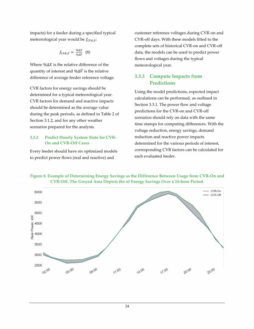
24
impacts) for a feeder during a specified typical
meteorological year would be 𝑓𝐶𝑉𝑅,𝑋:
𝑓𝐶𝑉𝑅,𝑋 = %∆𝑋
%∆𝑉 (8)
Where %∆𝑋 is the relative difference of the
quantity of interest and %∆�̅� is the relative
difference of average feeder reference voltage.
CVR factors for energy savings should be
determined for a typical meteorological year.
CVR factors for demand and reactive impacts
should be determined as the average value
during the peak periods, as defined in Table 2 of
Section 3.1.2, and for any other weather
scenarios prepared for the analysis.
3.3.2 Predict Hourly System State for CVR-
On and CVR-Off Cases
Every feeder should have six optimized models
to predict power flows (real and reactive) and
customer reference voltages during CVR-on and
CVR-off days. With these models fitted to the
complete sets of historical CVR-on and CVR-off
data, the models can be used to predict power
flows and voltages during the typical
meteorological year.
3.3.3 Compute Impacts from
Predictions
Using the model predictions, expected impact
calculations can be performed, as outlined in
Section 3.3.1. The power flow and voltage
predictions for the CVR-on and CVR-off
scenarios should rely on data with the same
time stamps for computing differences. With the
voltage reduction, energy savings, demand
reduction and reactive power impacts
determined for the various periods of interest,
corresponding CVR factors can be calculated for
each evaluated feeder.
Figure 8. Example of Determining Energy Savings as the Difference Between Usage from CVR-On and
CVR-Off. The Greyed Area Depicts the of Energy Savings Over a 24-hour Period.
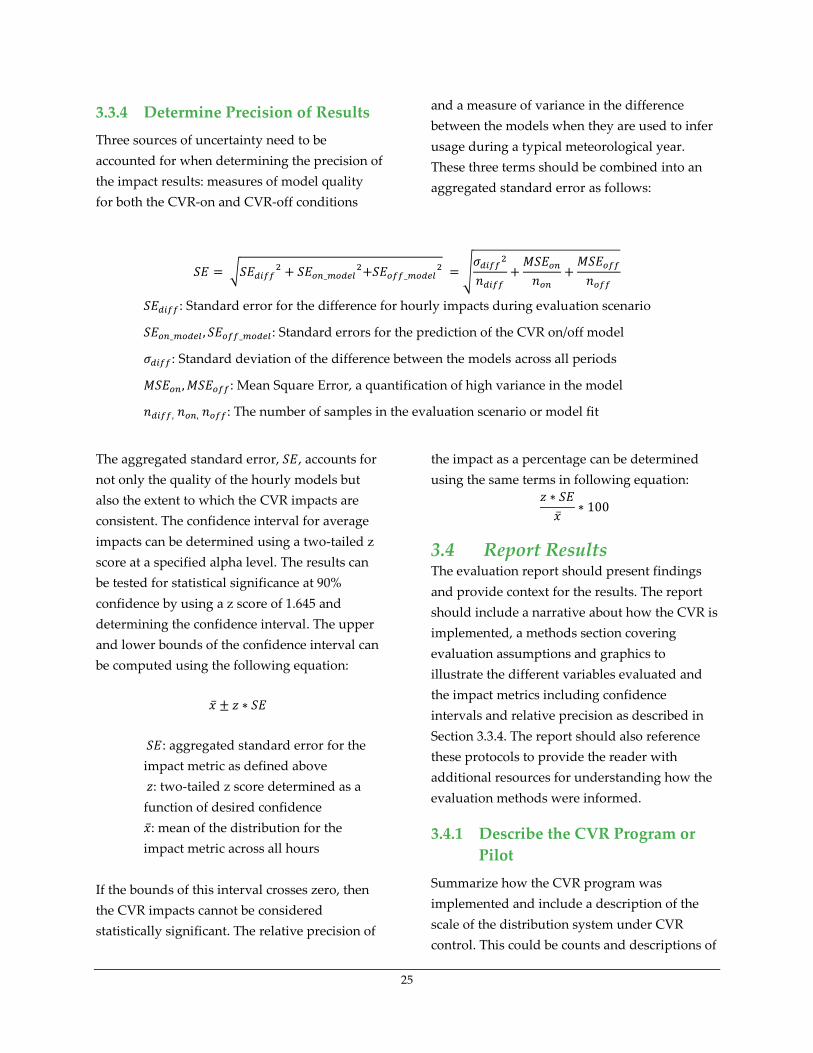
25
3.3.4 Determine Precision of Results
Three sources of uncertainty need to be
accounted for when determining the precision of
the impact results: measures of model quality
for both the CVR-on and CVR-off conditions
and a measure of variance in the difference
between the models when they are used to infer
usage during a typical meteorological year.
These three terms should be combined into an
aggregated standard error as follows:
𝑆𝐸 = √𝑆𝐸𝑑𝑖𝑓𝑓2 + 𝑆𝐸𝑜𝑛_𝑚𝑜𝑑𝑒𝑙
2+𝑆𝐸𝑜𝑓𝑓_𝑚𝑜𝑑𝑒𝑙2 = √
𝜎𝑑𝑖𝑓𝑓2
𝑛𝑑𝑖𝑓𝑓
+𝑀𝑆𝐸𝑜𝑛
𝑛𝑜𝑛
+𝑀𝑆𝐸𝑜𝑓𝑓
𝑛𝑜𝑓𝑓
𝑆𝐸𝑑𝑖𝑓𝑓 : Standard error for the difference for hourly impacts during evaluation scenario
𝑆𝐸𝑜𝑛_𝑚𝑜𝑑𝑒𝑙 , 𝑆𝐸𝑜𝑓𝑓_𝑚𝑜𝑑𝑒𝑙 : Standard errors for the prediction of the CVR on/off model
𝜎𝑑𝑖𝑓𝑓 : Standard deviation of the difference between the models across all periods
𝑀𝑆𝐸𝑜𝑛 , 𝑀𝑆𝐸𝑜𝑓𝑓 : Mean Square Error, a quantification of high variance in the model
𝑛𝑑𝑖𝑓𝑓, 𝑛𝑜𝑛, 𝑛𝑜𝑓𝑓: The number of samples in the evaluation scenario or model fit
The aggregated standard error, 𝑆𝐸, accounts for
not only the quality of the hourly models but
also the extent to which the CVR impacts are
consistent. The confidence interval for average
impacts can be determined using a two-tailed z
score at a specified alpha level. The results can
be tested for statistical significance at 90%
confidence by using a z score of 1.645 and
determining the confidence interval. The upper
and lower bounds of the confidence interval can
be computed using the following equation:
�̅� ± 𝑧 ∗ 𝑆𝐸
𝑆𝐸: aggregated standard error for the
impact metric as defined above
𝑧: two-tailed z score determined as a
function of desired confidence
�̅�: mean of the distribution for the
impact metric across all hours
If the bounds of this interval crosses zero, then
the CVR impacts cannot be considered
statistically significant. The relative precision of
the impact as a percentage can be determined
using the same terms in following equation:
𝑧 ∗ 𝑆𝐸
�̅�∗ 100
3.4 Report Results The evaluation report should present findings
and provide context for the results. The report
should include a narrative about how the CVR is
implemented, a methods section covering
evaluation assumptions and graphics to
illustrate the different variables evaluated and
the impact metrics including confidence
intervals and relative precision as described in
Section 3.3.4. The report should also reference
these protocols to provide the reader with
additional resources for understanding how the
evaluation methods were informed.
3.4.1 Describe the CVR Program or
Pilot
Summarize how the CVR program was
implemented and include a description of the
scale of the distribution system under CVR
control. This could be counts and descriptions of

26
feeders, transformers, customers or other
geographic metrics defining the scale of the
operation. Name the CVR software vendor and
any other products or companies involved with
the ongoing operation of the system. List the
dates of major milestones for the CVR system’s
testing and operation.
3.4.2 Describe Evaluation Process and
Assumptions
Outline the series of steps taken to compile and
process the dataset, fit and optimize the system-
state models and calculate the evaluation
metrics. Declare the data sources and the time
periods of all historical data used. Specify how
any weather scenarios beyond the standard
IESO peak definitions were constructed or
sourced. List filters used to cleanse the data, and
remark on the quantity of data that needs to be
dropped or modified because of quality
concerns. State the regression model type used,
identify the process used to produce additional
independent variables and describe how the
prediction quality of the models was validated
and optimized.
3.4.3 Share Plots of Historical,
Scenario and Predicted Data
Use graphics to reinforce the conclusions that
will be drawn from the tabulated impact
metrics. Identify the sources of all plotted data
and make sure the reader understands how the
presented data fit into the overall evaluation
process. Historical data should be plotted first
and should include power flow, voltage and
weather data from actual measurements taken
during the evaluation period. Scenario data
would be shown next and include typical
meteorological year data for expected energy
impacts, subsets for the peak period definitions
and other weather scenarios for expected
demand impacts. Finally, plots for predicted
power flows and voltages should be shown. It
would also be appropriate to produce
illustrative plots of underlying evaluation
metrics, such as expected cumulative energy
usage during a typical meteorological year or
hourly voltage profiles by season from CVR-on
and CVR-off cases. Figure 9 below shows an
example of average hourly energy usage for
when CVR is either on or off.
Figure 9. Example of Average Hourly Energy Usage Over a Year for CVR On vs Off

27
3.4.4 Present Expected Savings by
Feeder
Prepare tables to present evaluation metrics for
all the feeders in the study and, optionally, by
substation, if multiple substations are under
consideration. Evaluation metrics, as defined in
Section 3.3.1, should be associated with the
typical meteorological year. Report average
voltage reduction, either total energy savings or
average demand savings and CVR factors as
applicable for each feeder. Additionally, NMBE
and CV(RMSE) should be reported for every
system-state model to convey a standardized
measure of the model performance. Refer to
Section 3.2.3 for these definitions. To present
modelling fit to out-of-sample predictions, share
percentiles of r-squared scores from cross-
validating the optimized models as well as
confidence intervals and relative precision as
defined in Section 3.3.4. Summarize how this
cross-validation was executed, including the
number of rounds and the sizing criteria for the
held-out sample.

28
4. Protocols for Alternating-
Periods Customer-Level
Impact Evaluations
This section presents protocols for evaluating
the energy and demand impacts of
implementing CVR using an alternating-periods
analysis at the customer level. In contrast to a
feeder-level analysis in which the power, energy
and impacts are determined at the substation, a
customer-level analysis determines how CVR
affects usage as measured by the customer
billing meters. An impact evaluation at the
customer level should be done in concert with
an impact evaluation at the feeder level, and it
has similar data and analysis requirements.
Read Section 3 first, and then return to this
section, which expands upon the workflow and
recommendations discussed at the feeder level.
Many of the steps are similar for both protocols,
and some text is repeated to provide sufficient
context.
Alternating periods means that the CVR system
controller operates the CVR software to cycle
between active (CVR-on) and inactive (CVR-off)
days. This set of protocols is structured as the
following five steps:
Step 1. Collect historical and typical-
year data; sum up customer hourly
energy usage for a group analysis and
prepare individual customer usage on a
daily basis.
Step 2. Develop models to describe the
voltage, reactive power and real power
flows during the alternating CVR-on
and CVR-off days
Step 3. Derive impact metrics (energy
savings, demand reduction, reactive
power impacts and CVR factors) from
the difference in voltage, reactive power
and real power between CVR-on and
CVR-off days for different scenarios at
the customer level
Step 4. Report results
Plan to produce annual expected energy
savings, peak demand impacts and CVR factors
for all customers as a group. Modelling every
customer separately should only be done on a
daily basis given the high variance in hourly
usage. Models are developed from historical
data from both CVR-on and CVR-off days.
These models will then be applied to the typical
meteorological year. Savings based on
meteorological scenarios for a typical year and
during defined IESO peak periods are called
expected savings.
The customer-level impact results may be paired
with results from a feeder-level impact
assessment to isolate CVR impacts in front of the
meter versus behind the meter. As desired, the
feeder-level impacts can also be determined at
nodes downstream from the substation. This
allows for loading impacts to be determined for
specific distribution equipment and line
segments.
4.1 Compile and Prepare
Dataset If feasible, conduct data preparation efforts for a
customer-level analysis at the same time as
feeder-level analyses for the customers’ circuits.
This is most applicable to the time stamp event
data from the CVR controller system, the feeder-
level voltage and the independent variables
defining the weather and other temporal
features.
4.1.1 Collect Data
Data will be required from multiple sources, and
these data may include sensitive information
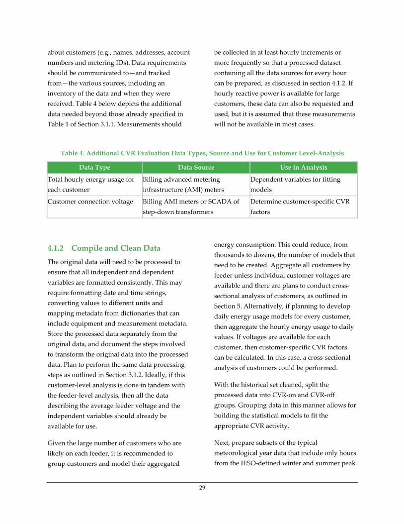
29
about customers (e.g., names, addresses, account
numbers and metering IDs). Data requirements
should be communicated to—and tracked
from—the various sources, including an
inventory of the data and when they were
received. Table 4 below depicts the additional
data needed beyond those already specified in
Table 1 of Section 3.1.1. Measurements should
be collected in at least hourly increments or
more frequently so that a processed dataset
containing all the data sources for every hour
can be prepared, as discussed in section 4.1.2. If
hourly reactive power is available for large
customers, these data can also be requested and
used, but it is assumed that these measurements
will not be available in most cases.
Table 4. Additional CVR Evaluation Data Types, Source and Use for Customer Level-Analysis
Data Type Data Source Use in Analysis
Total hourly energy usage for
each customer
Billing advanced metering
infrastructure (AMI) meters
Dependent variables for fitting
models
Customer connection voltage Billing AMI meters or SCADA of
step-down transformers
Determine customer-specific CVR
factors
4.1.2 Compile and Clean Data
The original data will need to be processed to
ensure that all independent and dependent
variables are formatted consistently. This may
require formatting date and time strings,
converting values to different units and
mapping metadata from dictionaries that can
include equipment and measurement metadata.
Store the processed data separately from the
original data, and document the steps involved
to transform the original data into the processed
data. Plan to perform the same data processing
steps as outlined in Section 3.1.2. Ideally, if this
customer-level analysis is done in tandem with
the feeder-level analysis, then all the data
describing the average feeder voltage and the
independent variables should already be
available for use.
Given the large number of customers who are
likely on each feeder, it is recommended to
group customers and model their aggregated
energy consumption. This could reduce, from
thousands to dozens, the number of models that
need to be created. Aggregate all customers by
feeder unless individual customer voltages are
available and there are plans to conduct cross-
sectional analysis of customers, as outlined in
Section 5. Alternatively, if planning to develop
daily energy usage models for every customer,
then aggregate the hourly energy usage to daily
values. If voltages are available for each
customer, then customer-specific CVR factors
can be calculated. In this case, a cross-sectional
analysis of customers could be performed.
With the historical set cleaned, split the
processed data into CVR-on and CVR-off
groups. Grouping data in this manner allows for
building the statistical models to fit the
appropriate CVR activity.
Next, prepare subsets of the typical
meteorological year data that include only hours
from the IESO-defined winter and summer peak

30
periods, as specified in Table 2 of Section 3.1.2.
These subsets will be used to prepare
independent variables for modelling voltage
and real power during the defined seasonal
system peaks. Next, prepare additional subsets
of data for additional weather scenarios. Refer to
Section 3.1.2 for additional guidance.
4.2 Create System-State Models This evaluation protocol relies on statistical
modelling to evaluate energy and demand
savings resulting from the CVR implementation.
Follow instructions as specified in Section 3.2.
4.2.1 Select an Appropriate
Regression Model
The models will define real power (and,
optionally, customer voltage) as the dependent
variables for each customer or customer group.
These state variables will be modelled on an
hourly or daily basis and will require that the set
of regression models (for energy consumption of
customers) are fit to data describing the weather
and other temporal effects. Refer to Section 3.2.1
for further guidance on regression model
selection.
4.2.2 Produce Additional
Independent Variables
Additional independent variables that can be
created from independent variable data should
be added to the dataset. One example is
converting the weather data into a computation
of cooling degree days or heating degree days.
These additional independent variables are also
called “engineered features” and are helpful
because they are repeatable and standardized
transformations of processed datasets that can
dramatically improve some models’ ability to
predict dependent variables of interest.
Depending on data available and the type of
regression model chosen, additional engineered
features improve the models’ accuracy for
predicting voltage and power flow. Refer to
Section 3.2.2 for further guidance on producing
additional independent variables. The complete
set of independent variables prepared for a
feeder-level analysis (i.e., weather and temporal
features) can also be used for the customer-level
analysis.
4.2.3 Optimize the Models
Optimizing the models requires both training
and testing. Train (i.e., fit) the model to a subset
of the historical dataset and then test the model
by seeing how well it predicts the held-out
historical data (i.e., the subset of data not used to
train the model). Plan to perform this training
and testing sequence multiple times with
different subsets of the historical data. This
process, called “cross-validation,” measures
prediction quality and is the most robust
method to determine that a model is fitting the
data well. The analysis framework used should
have cross-validation functionality built directly
into the modelling toolkit. At the end of the
cross-validation process, the validation scores
for each held-out dataset will illustrate how well
the model fits the dataset. Refer to Section 3.2.3
for guidance on model optimization.
4.3 Determine Customer-Level
Savings
4.3.1 Finalize Evaluation Metrics
The following evaluation metrics, as discussed
in Section 2, are the key metrics for determining
the impacts of implementing CVR. For complete
definitions and equations of the following
impact metrics, refer to Section 3.3.1.
Average Voltage Reduction: The average
difference between voltages from the CVR-off

31
models and CVR-on models. This can either be
associated with the average voltage of the feeder
(which should be used for customer groups) or
with the individual customer voltage. Average
voltage reduction should be calculated for both
the whole typical meteorological year and for
the specific IESO peak periods.
Total Energy Savings: The quantity of customer
energy usage that the CVR-off model predicts
would have been used beyond what was
predicted for the CVR-on case for a typical
meteorological year. To normalize across all
customer, energy savings should be determined
as a relative rather than absolute value.
Average Demand Reduction: The average
difference in real demand between the CVR-on
and CVR-off models during the IESO peak
periods if modeling usage on an hourly basis. To
normalize across all customers, demand
reduction should be determined as a relative
rather than absolute value.
CVR Factors: CVR factors should be calculated
by normalizing the modelled relative reductions
in energy demand and by the corresponding
relative reductions in voltage. If the power flows
of the customers are modelled individually, then
CVR factors can be reported for every customer
and the %∆�̅� should correspond to the modelled
voltages for the customer’s interconnection.
CVR factors for energy savings should be
determined for a typical meteorological year.
CVR factors for demand should be determined
as the average value for the typical year and
during the peak periods, as defined in Table 2 of
Section 3.1.2.
4.3.2 Predict System State for CVR-
On and CVR-Off Cases
Every customer or customer group should have
one optimized model to predict power flows
during CVR-on and CVR-off days. With these
models fitted to the complete sets of historical
CVR-on and CVR-off data, the models can be
used to predict power flows during the
evaluation periods of interest (typical
meteorological year, prepared peak periods, any
additional weather scenarios). If modelling
customers individually for a cross-sectional
analysis, also predict hourly voltages for each
customer.
4.3.3 Compute Impacts from
Predictions
Using the model predictions, expected impact
calculations can be performed, as outlined in
Section 3.3.1. The power flow of customers and
feeder-level voltage predictions for the CVR-on
and CVR-off scenarios should rely on data with
the same time stamps for computing differences.
With the feeder-level voltage reduction, and
customer energy savings and demand reduction
impacts determined for the various periods of
interest, corresponding CVR factors can be
calculated.
4.3.4 Determine Precision of Results
The standard error for the average relative
impacts among each group customers
should be calculated using the following
formula:
𝑆𝐸 = √𝜎2
𝑛𝑠𝑖𝑡𝑒𝑠
𝑆𝐸: standard error for the average
impacts on the group of customers

32
𝜎2: variance among customers’ relative
reduction values
𝑛𝑠𝑖𝑡𝑒𝑠: number sites included in the
treatment group
The confidence interval for average impacts can
be determined using a two-tailed z score at a
specified alpha level. Determine statistical
significance, confidence intervals and relative
precision using the equations defined above in
section 3.3.4
4.4 Report Results An evaluation report of customer-level impacts
should be presented along with the
accompanying feeder-level impacts. Follow the
reporting instructions specified in Section 3.4.
Results for customer groups or isolated
distribution equipment can be presented in the
same fashion as feeder-level results, except that
reactive power and demand impacts may not be
available. If conducting individual customer
impact evaluations, then it may not be possible
to present modelling fits for every single
customer as this level of granular detail is too
exhaustive for a impact report. In such cases,
report distribution statistics of modelling fits.
Present the average impacts determined for each
customers on each feeder and whether results
were statistically significant along with
confidence intervals as described in Section
4.3.4. A complete set of impacts for every
customer can be shared in a workbook.

33
5. Protocols for Cross-
Sectional Analysis with
Feeders and Customers
The preceding protocols define the steps
necessary to determine CVR impacts for specific
feeders and customers. If multiple feeders have
been included in the analysis, or if customers
were modelled individually, there is an
additional opportunity to quantify trends across
the group to see if certain characteristics are
strongly correlated with CVR factors. The
results from this cross-sectional analysis could
be used to estimate CVR impacts on other
systems for which the same characteristics are
also known. In this way, the results from piloted
CVR implementations can be used to inform
where the next best opportunities for CVR may
be. The quality of these correlations will be
highly dependent on which characteristics are
available to describe the feeders and the
customers.
5.1 Compile and Prepare
Dataset Sometimes called “second-stage” analyses,
cross-sectional analyses build upon the results of
previous analyses that have already determined
impacts at the feeder or customer level.
Therefore, it is assumed that protocols as
outlined in sections 3 and 4 have already been
followed, and that CVR factors for feeders and
individual customers have been calculated.
These CVR factors can be used from different
pilots, programs, utilities and geographic
regions, but the method for determining CVR
factors should be the alternating-periods
method across all cases.
5.1.1 Collect Data
The impact metrics for all feeders or customers
must be compiled. Additional characteristics
that will be used as features to describe these
systems then need be requested and compiled.
Table 5 provides examples of features that may
be available for this type of analysis. Compile
characteristic independent variables for a cross-
sectional regression across all systems in the
group.
5.1.2 Compile and Clean Data
Every feeder or customer will need a unique
row in a data table that includes the impact
results and all descriptive features. Numeric
features can be included with no modification.
Categorical features will need to be turned into
several columns of true/false values
(represented by 1 and 0, respectively) that
represent whether that instance is part of the
corresponding categories. These additional
variables are sometimes called “dummy
variables.” In this way, categorical data can be
included in the cross-sectional regression.
Methods employed to determine CVR factors
need to be consistent for all instances of feeders
and all instances of customers, as defined by the
protocols in the previous sections. Only combine
CVR factors produced from evaluations
following the alternating-periods method in a
cross-sectional analysis. Remove from the
compiled dataset all instances that do not meet
this criterion.

34
Table 5. Examples of Features that May be Available for Cross-Sectional Analysis
Numerical Features1
Feeder Customer
% Facility types
% of measure or program participation
Total square footage of all customers
Average annual load
Voltage base of feeder
Total length of feeder
Heating and cooling degree days of typical
meteorological year (if different scenarios were used
across the set of feeders)
Available demographic information
Average annual consumption
Seasonal peak demands
Square footage of building(s)
Heating and cooling degree days of typical
meteorological year (if different scenarios were used
across the set of feeders)
Number of residents
Number of workers
Capacity of distributed generation or energy
storage
Categorical Features1
Feeder Customer
CVR control vendor
Local distribution company
CVR control vendor
Facility type
Historical participation in energy efficiency or
demand management program
1. Essential features to include in this analysis have been italicized.
5.2 Correlate Features with
Impacts With all the data prepared, it is now possible to
fit a multivariable linear regression to estimate
CVR impacts based on either feeder or customer
characteristics. Figure 10 below presents the
complete equation showing how the compiled
dataset will be used to determine optimal
coefficients (𝜷𝒒, 𝜸𝒌) by minimizing the
regression residual (𝜺𝒋) for all systems in the
sample. Coefficients should be optimized using
ordinary least squares (OLS) methodology. The
determined coefficients as a set represent the
cross-sectional weights given to each
characteristic representing how it would predict
for CVR factors when fitting the regression. The
coefficients can be used in Equation 11 (shown
in Figure 10) to predict the impact metric for an
out-of-sample system (without the residual error
term that cannot be determined). For example, if
annual energy usage, building square footage
and facility type were used as features to
determine cross-sectional coefficients for peak
demand reduction CVR factors, then the peak
demand reduction CVR factor could be
estimated using those fit coefficients for a
facility that has never received CVR if the
annual energy usage, building square footage
and facility type were known.

Appendix A. Literature Review 35
Figure 10. Linear Regression for Cross-Sectional Analysis
5.3 Report Results The results from a cross-sectional analysis
should either accompany a report for a specific
CVR implementation or should reference the
reports from where results are being used. If
using CVR factors prepared by other evaluators,
then provide context and references for those
results. This would include a narrative about
how the CVR was implemented, a summary of
methods covering evaluation assumptions and
the final impact metrics. Finally, reference these
protocols to provide the reader with additional
resources for understanding how the cross-
sectional method was informed.
5.3.1 Describe Process and
Assumptions
Outline the series of steps taken to compile the
dataset and conduct the linear regression.
Declare the data sources and produce tables
summarizing the features used to characterize
the feeders or customers. List filters used to
cleanse the data, and remark on the prediction
quality of the cross-sectional model. State any
methods employed to optimize variables used
for the regression.
Additionally, NMBE and CV(RMSE) should be
reported for the cross-sectional models to
convey a standardized measure of the model
performance. Refer to Section 3.2.3 for these
definitions.
5.3.2 Share Plots and Tables of
Feature Data
Use tables and graphics to communicate the
diversity and distribution of feature values and
characteristics among the population of systems
being analysed. This should include scatter plots
and histograms. Also include histograms of
𝑌𝑗 = ∑ 𝛽𝑞𝑥𝑞𝑗𝑞 + ∑ 𝛾𝑘𝐼𝑘𝑗𝑘 + 𝜀𝑗 (11)
𝑗 = identifier for each system (feeder/customer) in cross-sectional analysis
𝑞 = identifier for numeric characteristic
𝑘 = identifier for binary categorical characteristic
𝒀𝒋 = CVR factor (for energy savings or real/reactive power reduction) for system 𝑗
𝑰𝒌𝒋 = 0/1 hot-encoded dummy variable. Equal to 1 if for system 𝑗 the characteristic 𝑘 is true. Equal to
0 if for system 𝑗 the characteristic 𝑘 is false.
𝒙𝒒𝒋 = value of the numerical characteristic 𝑞. Let 𝑥0𝑗, the first term of this vector, equal 1 for all
premises so that 𝛽𝑜 serves as an intercept term
𝜷𝒒, 𝜸𝒌 = coefficients determined by the regression
𝜺𝒋 = regression residual for system 𝑗

Appendix A. Literature Review 36
expected impact metrics being used to fit the
regression.
5.3.3 Present Cross-Sectional
Coefficients
Prepare tables to present the cross-sectional
coefficients determined through the OLS linear
regression for each expected impact metric. Be
sure to make it clear when coefficients are
positive or negative. Coefficients for numerical
characteristics should include the corresponding
units (e.g., kWh/square foot), while categorical
coefficients for dummy variables should have
units of the impact metric (e.g., kWh). Comment
on why certain variables may be strongly
correlated with CVR factors and why they may
be having a positive or negative impact. Offer
suggestions on how these coefficients can be
used by utility system planners to identify other
feeders that would be good candidates for CVR.

Appendix A. Literature Review A-1
Literature Review Appendix A.
Relevant literature covering the theoretical
potential of CVR implementation across North
America:
D. Pinney, "Costs and Benefits of
Conservation Voltage Reduction," U.S.
DOE/NETL, Arlington, Virginia, 2014.
K. Schneider, "Evaluation of
Conservation Voltage Reduction (CVR)
on a National Level," U.S. Department
of Energy, Oak Ridge, TN, 2010.
R. Singh and F. Tuffner, "Effects of
distributed energy resources on
conservation voltage reduction (CVR),"
IEEE, Detroit, MI, USA, 2011.
R. Scalley and D. Kasten, "The Effects of
Distribution Voltage Reduction on
Power and Energy Consumption," IEEE
Transactions on Education , vol. 24, no. 3,
pp. 210-216, 1981.
Relevant literature covering the evaluated
impact of CVR implementation across North
America.
M. Diaz-Aguiló, "Field-Validated Load
Model for the Analysis of CVR in
Distribution Secondary Networks:
Energy Conservation," IEEE Transactions
on Power Delivery, vol. 28, no. 4, pp.
2428-2436, 2013.
R. Griffith, "Voltage and Reactive Power
Optimization (Smart Grid Pilot Project,
Final Report)," PG&E, 2016.
K. Cooney, D. Greenberg, F. Stern and
P. Higgins, "Avista Utilities’
Conservation Voltage Reduction
Program Impact Evaluation," Avista
Utilities, 2014.
NREL, "Whole-Building Retrofit with
Consumption Data Analysis Evaluation
Protocol," in The Uniform Methods
Project: Methods for Determining Energy
Efficiency Savings for Specific Measures,
2013, pp. 4.7.12, Page 8-19.
M. Messenger, "Verification of the
Energy Saving Impacts of the Potomac
Edison CVR Program," Itron, Davis, CA,
2014.
Regional Techincal Forum, “Automated
CVR Protocol No. 1: Procotol Document
v1.1,” 2004
S. Lefebvre and G. Gaba, "Measuring the
Efficiency of Voltage Reduction at
Hydro-Quebec Distribution," IEEE
Power and Energy Society General Meeting,
no. Conversion and Delivery of
Electrical Energy in the 21st Century,
2008.
US EPA “Conservation Voltage
Reduction/Volt VAR Optimization
EM&V Practices,” 2017


