This is the final version (unedited) of the paper published in Transportation Journal 

Zhao, Y., Triantis, T.,  Edara, P. Evaluation of Travel Demand Management Strategies: A Microscopic Traffic Simulation Approach in: Transportation Journal, Vol. 37, No. 3, pp. 549‐571, 2010.   

 

1

Evaluation of Travel Demand Strategies: A Microscopic Traffic Simulation

Approach

Y. Zhaoa, K. Triantisa∗, P. Edarab

a System Performance Laboratory, Grado Department of Industrial and Systems Engineering, Northern Virginia Center, Virginia Tech, 7054 Haycock Road, Falls Church, VA 22043-2311

b Department of Civil and Environmental Engineering, University of Missouri-Columbia, E3502

Lafferre Hall, Columbia MO 65211

Abstract

This research investigates the design and impact of a new travel demand management

approach, namely the Downtown Space Reservation System (DSRS), using a microscopic

traffic simulation approach executed in VISSIM. The DSRS is part of a Travel Demand

Management (TDM) strategy that is designed to mitigate traffic congestion in a downtown urban

setting. The simulation is conducted according to an experimental design procedure for a

revised road network representing downtown Boise, Idaho. The issues that are tested in the

simulation include: (1) whether the DSRS improves traffic performance when compared with the

case without the DSRS; (2) how the DSRS performs compared with a reservation system that

uses a First Come First Serve (FCFS) principle; and (3) how the specific DSRS parameters

(such as, the relative importance of throughput versus revenue generation) influence network

system performance. Conclusions and future research recommendations are provided based

on the insights from the simulation modeling work.

Keywords: Travel demand management; Trip reservation; Traffic simulation; Transportation performance measurement; Urban network

∗ Corresponding author; Tel.: +1 703 538 8431/8446; fax: +1 703 538 8450 Email address: triantis@vt.edu

2

1.0 Introduction

Various Travel Demand Management (TDM) strategies have been proposed to tackle

congestion problems, and trip reservation is one of them. Zhao et al. (2009) developed a trip

reservation system, named the Downtown Space Reservation System (DSRS). It is a

transportation strategy developed for the purpose of congestion mitigation, especially for the

center of a city or Central Business District (CBD). Building upon the initial development of the

DSRS, this paper will present a microscopic traffic simulation model together with a simulation

experimental design scheme for the purpose of evaluating performance of this TDM strategy.

The DSRS is a rather new concept in the realm of TDM strategies and has not yet been

implemented in practice. A transportation system is a complex system involving different

stakeholders including the government, transportation agencies and the public. To implement

the DSRS, research is needed with respect to how well the DSRS will work and additional

research is needed to find out what is needed to gain support from various stakeholder groups.

So far research has only proposed basic concepts when defining reservation systems as

mechanisms to mitigate traffic congestion. This research builds a simulation model to address

the evaluation issues of such a system. Multiple experiments conducted within the context of

the simulation model show the effects of different system parameters and policies on network

performance and also assist decision makers and analysts in gaining more insights about the

relationships among various system components and in predicting system performance under

various conditions.

This research contributes to the literature in two ways. First, from a transportation

planning point of view, the proposed simulation approach provides a mechanism to illustrate

advantages of the DSRS. It facilitates the promotion of the system and communicates the

possible impacts of the system to potential stakeholders. Second, this research facilitates the

DSRS design process. Findings and insights derived from simulation results can be used for

further modification and improvement of the DSRS.

3

The remainder of this paper is organized as follows: Section 2 presents a literature

review of typical microscopic simulation applications in transportation, indicating the possibilities

and challenges in our application. The DSRS is briefly introduced in Section 3. Section 4

describes the simulation network used in this paper along with the simulation experiments. The

results of the simulation experiment are discussed and analyzed in Section 5. Implementation

issues of the DSRS are discussed in Section 6. Finally, in Section 7, conclusions are drawn

and future research recommendations are provided.

2.0 Simulation in Transportation Studies

Simulation is widely used in transportation. There are various traffic simulation

applications including (1) evaluation of signal control strategies, (2) analysis of equilibrium in

dynamic assignment, (3) analysis of corridor design alternatives, and (4) testing new concepts

(Lieberman and Rathi 1992). This work falls under the fourth area of testing a new concept,

which is a research thrust that has been pursued in the literature. Rathi and Lieberman (1989)

used a traffic simulation model to test metering control along the periphery of a congested urban

area to mitigate the congestion within the area. This early work illustrated the value of testing

new “high risk” ventures with simulation without exposing the public to possible adverse

consequences. Similarly, Ben-Akiva et al. (2003) evaluated four types of traffic control

strategies - access control, route control, lane control and integrated control - using a

microscopic simulation approach. Simulation is also used in the evaluation of intelligent

transportation systems (ITSs) (Barcelo and Codina 2005; Boxill and Yu 2000).

Microscopic simulation related to an urban transportation network is more complicated

than modeling an ordinary isolated intersection or a road segment due to the high level of detail

and the combination of different kinds of intersections and road network links. Micro-simulation

models are limited in scope and scale (i.e., in terms of the network size with respect to links,

nodes, and number of vehicles). Although Rakha et al. (1998) demonstrated the feasibility of

4

constructing and calibrating a large scale network at the microscopic level in the Salt Lake area,

the authors acknowledged the challenge of building such a large network. They emphasized

that the data collection and coding exercise is substantially intensive. The successful use of

micro-simulation is commonly limited to relatively small size networks (Kitamura and Kuwahara

2005). Nevertheless, due to the development of computer technology and the growing

popularity of the micro-simulation, the effort needed to run a micro-simulation will be reduced in

the near future.

3.0 The Downtown Space Reservation System (DSRS)

With the DSRS, travelers who want to drive in a designated downtown area have to

book their time slots before they make their trips. Reservation requests can be submitted

through different channels, i.e. internet, phone, and local stores. The transportation authority,

who administers and supervises the DSRS, allocates the time slots to different travelers based

on the availability of resources (i.e., road network capacity) and other criteria such as vehicle

classes and reservation revenue. Only those who get permission from the transportation

authority can drive in the downtown area during the requested time period. The rejected trips

are assumed to be accommodated by other modes such as walking, biking or public transit.

The DSRS process is depicted in Figure 1.

Figure 2 illustrates how monitoring the system would work in the field and how traffic

data could be collected. A similar monitoring system has been successfully implemented in

Stockholm (IBM, 2007). The system works in the following way:

1. The vehicle breaks the first laser beam, triggering the transceiver aerials in step 2;

2. The transceiver signals the vehicle’s onboard transponder, capturing the time and date;

3. At the same time, a camera photographs the vehicle’s front license plate;

4. The vehicle breaks the second laser beam, triggering the second camera in Step 5;

5. The second camera photographs the rear license plate without the vehicle slowing down;

5

6. The vehicle information (including time, date, and license number) is fed back to the

central computer and is confirmed with the stored reservation data to see whether the

current vehicle is in the booking system.

Figure 1: The Downtown Space Reservation System

Figure 2: Monitoring the System in Field

The proposed DSRS consists of two modules, an offline optimization module and an

online decision making module (neural network module). In the offline module, an optimization

6

problem is solved based on historical travel information. Multiple objectives are incorporated in

the optimization problem, i.e. the total number of people that the transportation system handles

during a certain time period and the revenue obtained from the reservation system. From a

travel demand management point of view, the mobility of people is improved by restraining the

excessive amount of automobiles entering the area. From an economic point of view, revenue

is maximized. This revenue can be used to finance public transportation systems as part of a

comprehensive travel demand management strategy.

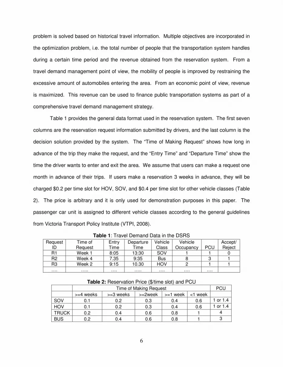
Table 1 provides the general data format used in the reservation system. The first seven

columns are the reservation request information submitted by drivers, and the last column is the

decision solution provided by the system. The “Time of Making Request” shows how long in

advance of the trip they make the request, and the “Entry Time” and “Departure Time” show the

time the driver wants to enter and exit the area. We assume that users can make a request one

month in advance of their trips. If users make a reservation 3 weeks in advance, they will be

charged $0.2 per time slot for HOV, SOV, and $0.4 per time slot for other vehicle classes (Table

2). The price is arbitrary and it is only used for demonstration purposes in this paper. The

passenger car unit is assigned to different vehicle classes according to the general guidelines

from Victoria Transport Policy Institute (VTPI, 2008).

Table 1: Travel Demand Data in the DSRS

Request ID

Time of Request

Entry Time

Departure Time

Vehicle Class

Vehicle Occupancy PCU

Accept/Reject

R1 Week 1 8:05 13:30 SOV 1 1 0 R2 Week 4 7.35 9:35 Bus 8 3 1 R3 Week 2 9:15 10.30 HOV 2 1 1 …. ….. …. ….. …. …. ….

Table 2: Reservation Price ($/time slot) and PCU Time of Making Request PCU

>=4 weeks >=3 weeks >=2week >=1 week <1 week

SOV 0.1 0.2 0.3 0.4 0.6 1 or 1.4

HOV 0.1 0.2 0.3 0.4 0.6 1 or 1.4

TRUCK 0.2 0.4 0.6 0.8 1 4

BUS 0.2 0.4 0.6 0.8 1 3

7

The objective function of the optimization module is formulated as:

Maximize Z = [Z1(X), Z2(X)] (1)

i

j

I

i

J

ji

j

i

jx

pcu

psgXZ ∑ ∑

= =

=

1 1

1 )( (2)

i

j

I

i

J

j

i

jm

M

m

i

m xapXZ ∑ ∑ ∑= = =

=

1 1 1

2)( (3)

Z1(X) stands for the people throughput objective and Z2(X) is the revenue objective. The multi-

objective problem is reduced to a single-objective problem using prior assessment of weights.

The weight w is equivalent to the identification of a desirable tradeoff between Z1 and Z2.

Equation (1) becomes: Maximize Z (w) = wZ1(X) + (1- w)Z2(X) (4)

Subject to the capacity constraints: TmCapcuxi

jm

i

j

I

i

J

j

i

j ,...,11 1

=≤∑ ∑= =

(5)

i

jpsg Total number of passengers in the vehicle for the j-th request of demand category i

i

jpcu The passenger car units of the vehicle for the j-th request of demand category i

i

mp The reservation price of time slot m for demand category i

C Transportation network capacity (Section 4.3)

=

otherwise 0,

interval time th-m the in included is i category demand of request th-j if 1,i

jma

=

otherwise 0,

accepted is icategory demand of request th-j if 1,i

jx

Each time slot is assumed to be a five-minute interval in this paper. The problem

defined by relations (4) and (5) is an integer programming problem. It can be solved using

CPLEX.

The reservation center could be opened several days before the trip’s schedule

departure time. The system operator has to make a decision whether to accept or reject a user

request at the time the user makes the request or within a reasonable time after receiving the

request. This decision making process is trivial task if the travel demand in the future is

deterministic. However, it is difficult to predict the future demand pattern in an accurate manner.

8

The operator has to make real-time decisions based on the information associated with the

cumulative requests at that instant, as he is unaware of the future requests. In order to take into

account the stochastic variations in travel demand, a neural network is used to construct the

online module. Assuming that we have hundreds of historical demand scenarios, we obtain

optimal solutions using CPLEX for each scenario. Given that artificial neural networks have the

ability to “learn from experience” (Teodorović and Vukadinović, 1998), they can learn from the

historical demand scenarios and the optimal solutions. From this learning process, the system

will be able to recognize a situation characterized by the number of reservations that already

have been made for each vehicle class during each time period and the corresponding revenue

obtained from the reservations. Therefore, when a new request comes in, the neural network

can rely on this historical information to provide a real time decision.

4.0 Simulation Experiments

4.1 Experimental Purposes

In the optimization module, people throughput and revenue maximization are explicitly

included in the optimization objective whereas measures like travel time and travel speed are

not. However, these measures are important for examining how the newly-introduced system

meets congestion mitigation goals. Additionally, measures such as these are easily

communicated to and understood by the public and transportation professionals. Traffic

simulation package VISSIM (PTV America, 2007) is used to provide performance measures for

system evaluation purposes.

4.2. Simulation Test-bed – the VISSIM Network

4.2.1 Description of the Network

The VISSIM network used in this research is part of the Downtown Boise Simulation

Study, which is provided in the VISSIM Software package. The network is modified to meet the

needs of this research. The reason for using an existing network rather than coding a new one

9

is that, the DSRS is developed for any general downtown network, and the network in the

Downtown Boise Simulation Study has the characteristics of a typical downtown area with many

intersections and short links (Zhao et al., 2009). It is a reasonable representation of typical

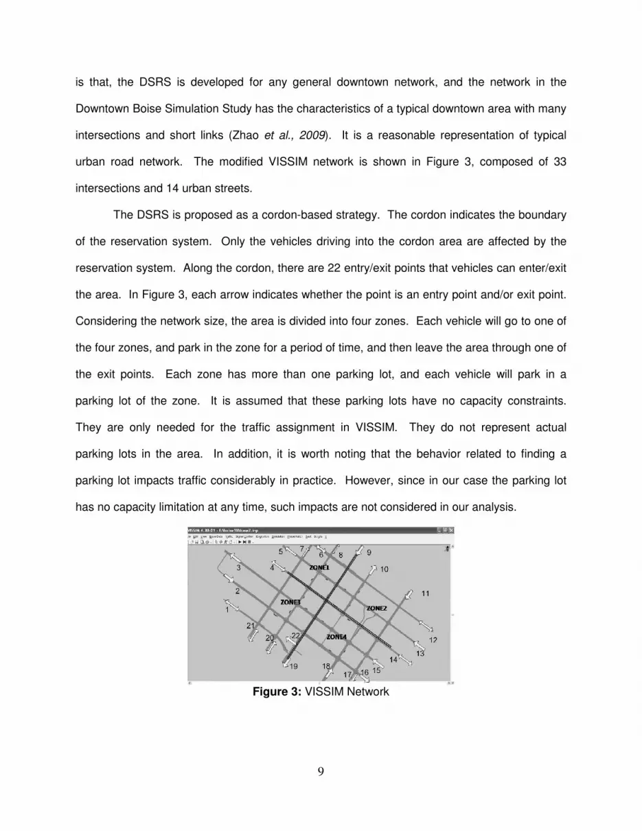
urban road network. The modified VISSIM network is shown in Figure 3, composed of 33

intersections and 14 urban streets.

The DSRS is proposed as a cordon-based strategy. The cordon indicates the boundary

of the reservation system. Only the vehicles driving into the cordon area are affected by the

reservation system. Along the cordon, there are 22 entry/exit points that vehicles can enter/exit

the area. In Figure 3, each arrow indicates whether the point is an entry point and/or exit point.

Considering the network size, the area is divided into four zones. Each vehicle will go to one of

the four zones, and park in the zone for a period of time, and then leave the area through one of

the exit points. Each zone has more than one parking lot, and each vehicle will park in a

parking lot of the zone. It is assumed that these parking lots have no capacity constraints.

They are only needed for the traffic assignment in VISSIM. They do not represent actual

parking lots in the area. In addition, it is worth noting that the behavior related to finding a

parking lot impacts traffic considerably in practice. However, since in our case the parking lot

has no capacity limitation at any time, such impacts are not considered in our analysis.

Figure 3: VISSIM Network

10

4.2.2 VISSIM Traffic Demand Inputs

The experiment in this research based on a VISSIM network of downtown Boise, which

was originally developed by PTV America, Inc. (PTV America, 2007). We adopted the existing

signal timing and roadway geometry. Travel demand distribution is generated by taking into

consideration the vehicle inputs originally used by PTV. The column “Production” contains the

“Vehicle Inputs (vehicles/hour)” from the original Boise VISSIM network. “Production Percent” is

computed as the ratio of entry points “Production” to the total production trips, for example for

entry point 1, the production percent is 100/6484=1.54%. In our experiment, trips are

distributed across the entry points according to the “Production Percent” values, and trips are

evenly distributed among the four zones according to the “Attraction Percent” values (Table 3).

In addition, a sensitivity analysis with respect to trip attraction rates where trips were not evenly

distributed among the four zones yielded similar results to the ones reported in this paper.

Table 3: Trip Generation

Entry Points ZONE1 ZONE2 ZONE3 ZONE4 Production

Production Percent (Production/Total Trips)

1 25 25 25 25 100 1.54% 2 191 191 191 191 764 11.78% 4 46 46 46 46 184 2.84% 6 167 167 167 167 668 10.30% 8 23 23 23 23 92 1.42% 9 200 200 200 200 800 12.34% 11 242 242 242 242 968 14.93% 12 121 121 121 121 484 7.46% 13 65 65 65 65 260 4.01% 14 75 75 75 75 300 4.63%

15 116 116 116 116 464 7.16% 18 225 225 225 225 900 13.88% 22 57 57 57 57 228 3.52% 20 25 25 25 25 100 1.54% 21 43 43 43 43 172 2.65%

Attraction 1621 1621 1621 1621 6484 Attraction Percent 25% 25% 25% 25%

Each vehicle stays in a zone for a period of time, and then chooses one of the exit points

to leave the downtown area. Figure 4 shows all the combinations of the entry and exit point

pairs. In this paper, we assume that people prefer to depart from the same point of entry or the

11

closest exit point to its entry point (Table 4). According to this assumption, for instance, vehicles

that enter through entry point #1 will leave through departure point # 1.

Figure 4: Vehicles Flow Chart

Table 4: Entry/Departure Pairs

Entry Points Departure Points 1 1 2 3 4 4 6 6 8 7 9 8

11 10 12 12 13 5 14 14 15 16 18 19 22 17 20 20 21 21

4.2.3 Network Capacity Determination

According to Zhao, et al. (2009) capacity of the road network (Figure 3) is computed as:

∑∑∈∈

==

Ai

iji

Ai

i

Akl

nn2

(6)

Where nA is the network capacity and link i belongs to the network A; li is the length of link I;kij is

the jam density of link i. Jam density is the condition of extremely high density that brings the

traffic on a roadway to a complete stop. In this research, we assume that under jam density

road conditions, vehicles stop in the road and are bumper-to-bumper. Therefore, the jam

density of a link can be formulated as:

AvgLenlAvgLen

l

ki

i

ij

1==

(7)

Where AvgLen denotes the average vehicle length for a standard car.

Equation (6) is rewritten as:

12

∑∑∑ ===

∈∈ i

i

Ai

i

Ai

i

A

AvgLen

lAvgLenl

nn22

1

(8)

Average vehicle length is computed from the data from Klaus Parking Systems, Inc. (2008).

The length of 87 different types car models is averaged, AvgLen = 196 (ft). Then the capacity of

the network (of Figure 3) is computed as 2550 PCUs.

4.3 Experimental Design

4.3.1 Experimental Hypotheses

The major hypothesis is that congestion will be mitigated and transportation performance

will be improved with the reservation system according to performance measures such as travel

time, congestion delay time and average speed. It is also worthwhile to look at the change of

total vehicle miles traveled as a system throughput. If there is no congestion, this measure

could be reduced with the DSRS, because without the DSRS more vehicle trips can be

accommodated by the network. On the other hand, if serious congestion exists, even if more

vehicles are allowed to travel in the network, the total miles they can travel could be less than

the case with the DSRS within the same time period. Furthermore, it is expected that with the

DSRS, transportation performance is more stable than it is without the DSRS.

The DSRS is different from the first come first serve (FCFS) reservation system. The

DSRS is expected to outperform FCFS in terms of people throughput and revenue maximization.

In addition, it is expected that changes in the relative importance of the throughput and revenue

objectives in the optimization module will also affect the network performance.

4.3.2 Experimental Procedure

Three experiments are set up according to the hypotheses:

• With and without the DSRS at different demand levels

Multiple demand scenarios are generated. These scenarios are controlled by the

parameter of average arrival rate λ. The arrival rate indicates the intensity of the travel demand

13

of the particular scenario. The process of vehicles entering the designated network is assumed

as a Poisson process with a known average rate λ. In this case, six arrival rates are chosen

indicating different levels of traffic demand (Table 5). These six arrival rates represent the traffic

conditions ranging from low, to moderate, and to extreme congestion. For each demand

scenario, the simulation runs twice, i.e., the simulation with the reservation system (Figure 5)

and the simulation without reservation system in place (Figure 6).

Table 5: Travel Demand Levels Parameter I II III IV V VI Arrival rate λ [Vehicles/3Hours] 7000 7200 7400 7600 7800 8000

• Reservation System: DSRS vs. FCFS

The major objective in this analysis is to compare performance of the DSRS versus the

reservation policy of FCFS. In the DSRS, decision-makers make sure that the capacity is

available first, and then check whether the current request maximizes system objectives. It is

still possible that the request will be rejected even if capacity is available because decision-

makers may expect that saving the current slot for a later request could maximize the system

objective. Under FCFS reservation, the total network capacity must still be considered and

reservation requests are honored on a first come first serve basis. However, a request will be

accepted as long as there is vacancy regardless of future possible trip requests.

• People throughput vs. revenue

As was stated previously, two objective function components (people throughput and

revenue) are involved in the DSRS and there is a tradeoff between the two components. In the

DSRS, weights are assigned to the two components indicating their relative importance. To

reflect how the weights affect the system performance, an experiment is conducted for one

demand scenario (λ=7000), where different weights are assigned to the two components.

14

Figure 5: Simulation Process with Reservation System

Figure 6: Simulation Process without Reservation System

4.3.3 Other Simulation Parameters

In this experiment, the DSRS is assumed to be operating only during the AM peak

period, when heavy traffic enters a downtown region. Some of the trip chains will fall out of this

AM peak period window. In such cases, only the portion of the trip chain that occurs during the

reservation period (in this case AM peak period) determines the available allocation capacity

and the reservation fees.

The stochastic nature of traffic flow is very important in the context of microscopic traffic

simulation. In VISSIM, many parameters are assumed to follow a distribution rather than have a

fixed value, such as the desired speed distribution. In order to capture the stochastic nature of

traffic flow, each demand input should be run multiple times with different random seeds to

obtain stochastically sound MOE values. A simulation run with one random seed is called a

15

simulation replication. The number of replications for each demand input depends on two

factors, i.e., the desired level of accuracy and simulation output variation across multiple runs.

We use the standard deviations of MOEs to illustrate the output variation in the simulation

experiment. All results presented in this paper are based on ten random seeds for each

demand scenario.

5.0 Simulation Outputs Analysis

5.1 Measures of Effectiveness

Outputs provided by VISSIM allow a wide range of MOEs at various levels of detail. The

selected measures in this paper are mostly defined at the network level, since our intention is to

improve the overall traffic condition for the entire network rather than a single intersection or link.

Delay time is one of the most important measures. In VISSIM, delay time is determined by

comparing the actual travel time with the ideal travel time. The ideal time is the time with free

flow speed and no signal control. The total delay is computed by subtracting the ideal travel

time form the real travel time. Meanwhile, average speed is used to indicate the average traffic

flow condition. Dwell times at stop signs and signals are included in the calculation of average

speed and delays. The measure of total path distance is essentially the total vehicle miles

traveled in the entire network during the simulation time horizon.

5.2 Simulation Convergence Test

Convergence is a key notion in dynamic traffic assignment. Since there is no agreement

among simulation experts whether dynamic assignment convergence is needed for the

simulation run with each random seed for the same demand input, this research starts with

conducting a convergence test before running the experiments proposed in Section 3. A

demand scenario with arrival rate λ =7000 is presented.

First, the dynamic assignment algorithm (DA) is run until it converges for a single

random seed (R1). The obtained routes are then entered into the simulation model and the

16

model is run for random numbers R2 to R10. These results are shown in Table 6. Next, the DA

algorithm is independently run for each random seed (R1 to R10) and allowed to converge.

These results are shown in Table 7.

Table 6: Convergence of One Random Seed MOEs R1 R2 R3 R4 R5 R6 R7 R8 R9 R10

Average delay time per vehicle [s] 562 565 574 560 546 572 566 574 573 571

Average speed [mph] 13 13 13 13 13 13 13 13 13 13 Total travel time [h] 325 323 329 322 320 326 324 328 331 325

Total Path Distance [mi] 4200 4181 4204 4196 4177 4179 4207 4201 4192 4179 Total delay time [h] 167 166 171 164 163 169 166 170 174 168

Table 7: Convergence of All Random Seeds

MOEs R1 R2 R3 R4 R5 R6 R7 R8 R9 R10 Average delay time per vehicle [s] 562 558 561 555 553 595 558 581 562 564 Average speed [mph] 13 13 13 13 13 13 13 13 13 13 Total travel time [h] 325 321 325 321 322 333 323 330 327 324 Total Path Distance [mi] 4200 4186 4207 4195 4177 4177 4202 4209 4208 4192 Total delay time [h] 167 164 167 163 165 176 165 172 169 167

The t-test (Table 8) suggests that the results of the two tables are very close, when

comparing the MOEs in the two tables (Tables 6 and 7). There is no significant difference

between the two cases. Therefore, in the following experiments, for any given demand input,

we conduct DA until it converges starting with any random seed. From there we test the

stochastic impacts on the MOEs by changing the random seeds.

Table 8: Convergence t-test (α=0.05)

Average delay time

per vehicle [s] Average

speed [mph] Total travel

time [h] Total Path

Distance [mi] Total delay

time [h] t Statistic 0.41 -0.40 0.13 -1.69 0.26 t Critical 2.26 2.26 2.26 2.26 2.26

5.3 Simulation Analysis I: With and Without the DSRS

Scenarios S1 through S6 show how the system performs under different demand

scenarios indicated by the traffic arrival rate (λ). To compare the system performance with and

without DSRS, measures such as average delay, average speed, total path distance and total

travel time are chosen and plotted in Figure 7. Under DSRS the system exhibits a more stable

trend according to the MOEs in Figure 7.

17

Total path distance without DSRS is indeed higher than it is with DSRS for the first five

scenarios. This is because under DSRS, fewer vehicles are allowed to travel within the network

(Table 9). If we consider the total path distance as the system throughput (indicating how many

vehicle miles will travel at this level of demand), we would arrive at the conclusion that the

system produces more vehicle miles without DSRS. In this sense, we might be better off

without DSRS. Nevertheless, one may also observe that starting with S5, the number of vehicle

miles begin to decline When the demand level increases where λ =8000 vehicles/3 hours

(demand scenario S6), the total path distance without DSRS begins to drop to a lower level than

it is with DSRS. The degradation of total path distance is due to the higher congestion level,

indicated by the extremely high average delay (1776 seconds) and low average speed (3mph).

For example, in demand scenario S6, 4812 vehicles trips entered the network in the case when

the DSRS is implemented, and 6284 vehicles entered the network without the DSRS. However,

the total path distance without the DSRS (3936) is lower than the distance with the DSRS (4114).

This is because even if there are more vehicle trips when there is no DSRS, many vehicles are

stuck in the network and not able to complete their trips.

On the other hand, average delay and average speed are observed to represent the

traffic flow conditions. Comparing the average delay time per vehicle, it is obvious that vehicles

experience less average delay under DSRS. Especially in the case where travel demand level

λ increases, the average delay under DSRS does not vary very much, but the average delay

without DSRS increases sharply. In addition, the average speed drops from 12 mph to 3 mph

indicating severe congestion.

18

Table 9: VISSIM Results

Parameters Entering Volume

Average delay time per

vehicle [s]

Average speed [mph]

Total travel time [h]

Total Path Distance

[mi]

Total delay

time [h]

S1 (λ=7000)

WRa 5602 524 13 309 4057 155

WOb 6886 721 12 404 4859 220

%c -27% 9% -24% -17% -29%

S2

(λ=7200)

WR 5794 485 13 285 3754 142 WO 6934 808 11 470 4841 287 % -40% 24% -39% -22% -51%

S3

(λ=7400)

WR 5685 517 13 303 3947 153 WO 6295 834 11 441 4917 255 % -38% 17% -31% -20% -40%

S4

(λ=7600)

WR 5673 520 13 301 3913 153 WO 5746 987 10 504 5185 308 % -47% 26% -40% -25% -51%

S5

(λ=7800)

WR 5724 532 13 305 3933 155 WO 6752 1367 6 950 4581 777 % -61% 124% -68% -14% -80%

S6

(λ=8000)

WR 4812 645 12 342 4114 187 WO 6284

1776 3 1507 3936 1359

% -64% 348% -77% 5% -86%

In order to illustrate the magnitude of the change of the selected MOEs with the DSRS

compared to the same network without DSRS, the percentage differences are plotted in Figure

8. It is clear from this Figure that the average speed increases from 9 percent to 348 percent

across the six scenarios from the DSRS scenarios to the non-DSRS scenarios. Total travel

time and average delay consistently decrease as demand increases. This is due to the way in

which VISSIM computes delay. The delay is the difference between the ideal travel time and

the actual travel time. The two MOEs are highly correlated.

a VISSIM measurements with DSRS

b VISSIM measurements without DSRS

c Percent change in VISSIM measurements when comparing WR with WO

19

Figure 7: Performance Comparison with and without the DSRS (S1-S6)

Figure 8: Performance Comparison with and without the DSRS

20

5.4 Simulation Analysis II- DSRS vs. FCFS

The intention of this set of simulation runs is to compare the performance of the DSRS

versus the FCFS reservation system. The ten demand instances with the same average arrival

rate (λ =7000 vehicles/period) are simulated. The travel demand instances are differentiated

from each other because of the stochastic nature associated with the arrival rate, entry/exit time,

and occupancy. As shown in Table 10, the total revenue obtained from the DSRS is higher than

the revenue from the case of FCFS (average of 17 percent), and the people throughput (total

number of people served) also improves on average about 10 percent.

Table 10: People Throughput and Revenue DSRS vs. FCFS

# of trips DSRS

Revenue

DSRS People

Throughput FCFS

Revenue

FCFS People

Throughput

Revenue Percent Change

People Throughput

Percent Change

i1 5949 22210.9 17522 19123 15945 16.15% 9.89%

i2 5953 21888.4 17826 18943.8 16615 15.54% 7.29%

i3 5913 21898.9 17306 18603.1 15870 17.72% 9.05%

i4 5840 22824 17642 19068.8 16039 19.69% 9.99%

i5 5889 21976.6 17765 18822.5 14708 16.76% 20.78% i6 5888 22376.8 17811 18896.4 16172 18.42% 10.13% i7 5938 22706.3 17822 19150.5 16303 18.57% 9.32% i8 5914 22322.6 17210 18898 15966 18.12% 7.79%

i9 5963 22081.2 18211 19482.5 16561 13.34% 9.96% i10 5871 22143.3 17622 19046.4 16362 16.26% 7.70%

Mean 5912 22243 17674 19004 16054 17.06% 10.19%

In terms of the traffic performance, we still consider the following MOEs: average delay

per vehicle, average speed, total travel time/distance, and total delay time (Table 11).

According to the results of the t-test (α=0.05), differences between these two cases are not

significant, and this indicates that there are no significant improvements of traffic conditions

(Table 12). This phenomenon is consistent with the fact that under both the DSRS and FCFS,

traffic flow is subject to the same capacity constraints. Therefore, the total number of vehicles

accepted is similar. However, even if the traffic conditions are similar, from the revenue

maximization and people throughput point of view, the DSRS still outperforms the case of FCFS.

21

Table 11: VISSIM Results DSRS vs. FCFS i1 i2 i3 i4 i5 i6 i7 i8 i9 i10 DSRS

Average delay per vehicle 566 579 571 552 574 558 563 547 669 548

Average speed 13 13 13 13 13 13 13 13 11 13 Total travel time 325 329 326 318 325 319 321 318 405 318

Total Path Distance 4192 4245 4218 4124 4181 4126 4157 4167 4142 4159 Total delay time 168 170 167 162 168 164 165 160 249 162

FCFS Average delay per

vehicle 548 543 542 529 571 561 550 548 568 550 Average speed 13 13 13 13 13 13 13 13 13 13 Total travel time 320 316 315 308 327 323 321 321 330 321

Total Path Distance 4173 4122 4099 4026 4193 4145 4157 4167 4242 4174 Total delay time 162 160 159 155 168 166 163 162 169 163

Table 12: t-test Results DSRS vs. FCFS (α=0.05)

Average delay per vehicle [s]

Average speed [mph]

Total travel time [h]

Total Path Distance [mi]

Total delay time [h]

t Stat 2.21 -1.06 1.36 0.95 1.36 t Critical 3.25 3.25 3.25 3.25 3.25

5.5 Simulation Analysis III-The Relative Importance of Throughput vs. Revenue

As mentioned previously, the objective function of the DSRS contains two components,

i.e., people throughput and revenue. The two components are assigned different weights

indicating their corresponding importance (Table 13). For example, when the weight is equal to

0.5, this indicates that the two elements are equally important, and 1 indicates the case that only

people throughput is considered while assigning a zero weight to revenue. Theoretically, as the

weight for people throughput increases, the total number of people should increase as well.

The second column of Table 13 shows this behavior. However, the increases are not very

noticeable until the weight is increased to 1. The revenue follows a decreased trend. However,

the degree of decrease of revenue (10 percent) is higher than the increase of the people

throughput (4 percent). This result indicates the compromise between the two criteria of people

throughput and revenue (Figure 9). To test the significance of the changes in people throughput

and revenue with respect to weights w, additional t-test was conducted to compare results for

22

weights 0.5 and 0.89, and 0.89 and 1 as shown in Table 14. The results indicate that the

differences in results for the three weights are statistically significant.

On the other hand, the resulting performance measures from the simulation runs (Table

15) demonstrate that the differences among the various weight configurations are not intuitively

obvious. This is a reasonable finding. Different weights may only influence which vehicle will

be accepted, while the total number of vehicles is mostly constrained by capacity. Thus, with

the same amount of travel demand in the network, the traffic conditions should perform similarly.

Therefore, it may not be necessary to impose a higher weight on the people throughput

even if one aims at increasing the people throughput, because the network improvement is

limited. By increasing the weight on the people throughput, we may not get much improvement,

but lose much more revenue. In this case, it may be not worthwhile to sacrifice the revenue in

order to gain a limited increase of the people throughput.

Figure 9: People Throughput and Revenue

23

Table 13: People Throughput and Revenue

Weight w # of people throughput Revenue # of accepted vehicles

0.50 17018 22529.5 5908 0.67 17443 22288.7 5937 0.75 17522 22210.9 5949 0.80 17572 22155.3 5946 0.83 17582 22147.4 5944 0.89 17604 22124.2 5940 0.91 17604 22124.2 5940 0.95 17638 22080.5 5939 0.97 17644 22050.3 5945 0.98 17661 21956.3 5953

1 17674 20401.7 5966

Table 14: t-test Results of W=0.5, 0.89, 1

Revenue # of people

w=0.89 vs. w=1 w=0.5 vs. w=0.89 w=1 vs. w=0.89 w=0.89 vs. w=0.5

w=0.89 w=1 W=0.5 w=0.89 w=1 w=0.89 w=0.89 w=0.5

Mean 22066 20101 22520 22066 17775 17678 17678 17020 Df 29 29 29 29

t Stat 16.41 30.74 17.87 41.56 P(T<=t) one-tail 1.62E-16 5.51E-24 1.7E-17 1.06E-27 t Critical one-tail 1.70 1.70 1.70 1.70 P(T<=t) two-tail 3.24E-16 1.1E-23 3.4E-17 2.13E-27 t Critical two-tail 2.05 2.05 2.05 2.05

Table 15: Performance Results for Different Weights

Weight w 0.50 0.67 0.75 0.80 0.83 0.89 0.91 0.95 0.97 0.98 1 Average delay per vehicle [s] 579 586 566 582 586 585 577 592 598 598 611 Average

speed [mph] 13 13 13 13 13 13 13 13 13 13 13 Total travel

time [h] 330 336 325 334 335 334 331 337 339 339 345 Total Path

Distance [mi] 4230 4316 4192 4315 4306 4297 4288 4326 4330 4326 4367 Total delay

time [h] 171 174 168 172 173 173 170 175 177 176 181

6.0 Implementation Issues Associated with the DSRS

To implement the proposed DSRS many implementation issues need to be addressed.

Some of the relevant issues are discussed below.

• Reserving spaces: The communication channel (s) via which travellers can make reservation

requests could include, telephone, internet, text messaging, among others. The time window

available to make a request also is a key variable. For example, the reservation system can

24

be opened 24 hours in advance and closed 1 hour prior to the actual departure times. The

size of this window depends on the request processing capabilities of the DSRS server.

• Early/Late arrivals: In the event that a vehicle arrives at its entrance (say freeway ramp)

before or after its scheduled arrival time the DSRS needs to have sufficient slack in the

system to accommodate such vehicles. This can be accomplished by setting aside a certain

portion of the entrance capacity to such arrivals. The early arriving vehicle can be issued a

warning in the first violation with repeat offenders being ticketed and/or preventing them from

making reservations for a certain number of days.

• Late departures: It may happen that the departure plans of travellers change after entering

the downtown region. This could happen for a variety of reasons – for example, a meeting

running late. Again, in the situations where drivers violate their original departure times these

may be treated the same way early/late arrivals are treated.

• Enforcement: License plate numbers provided by motorists while reserving spaces can be

used for enforcement purposes. These numbers can be read at highway speeds with the

current technology and processed in milliseconds. If the number does not match the system

accepted number for that time interval then a violation ticket is issued. To detect the number

of occupants inside the vehicle, technology such as infrared and laser can be used (e.g.

Forth road bridge in Scotland has tested such equipment for use in a variable pricing project

in 2007. The system gives discounts to car pools based on the number of occupants.)

• Daily commuters: People who work in downtown and commute on every week day could be

treated in a different way. A portion of the total capacity can be devoted to drivers that are

willing to make reservations for a longer period of time (e.g., few months to up to a year).

Since they help reduce the uncertainty in demand, such requests can be given preferential

treatment, for example, reducing the reservation price.

25

• Trip cancellations/No-shows: The DSRS should also establish a policy on treating trip

cancellations and drivers that don’t show up for their trips. Assigning penalties on future

reservations is one way of dealing with it. Drivers missing their reservations for valid reasons

such as a medical emergency may be allowed to show the necessary proof to get the penalty

waived. It is to be noted that these are just potential ideas of how to deal with such

violations. It is entirely up to the agency implementing the DSRS to develop such a policy.

• Request rejections and re-requests: Travellers whose travel requests are turned down for a

certain time interval may keep checking (re-requests) in hope of someone cancelling their

trips or may choose to reserve for the next available departure time. The number of re-

requests is an important factor for the design of the reservation server and should be taken

into account to avoid service outages due to the overloading of the server.

• Privacy issues: Travellers may be asked to provide their license plate numbers during

reservations. The agency should take sufficient care not to disclose the identity of drivers.

This situation is very similar to the automated tolling applications around the world and may

not be a major implementation issue.

7.0 Conclusions and Future Research

The new TDM strategy, the Downtown Space Reservation System is evaluated using

microscopic traffic simulation. Three sets of simulation analyses are presented. According to

the simulation experiment in this paper, the DSRS can markedly improve traffic conditions as

compared to the no-control case, especially in an area with high congestion levels. Congestion

is highly sensitive to the total number of vehicles in the network after the total demand reaches

a certain level (about 7600 vehicles in the case presented in this research). A small amount of

extra vehicles could lead to great degradation in network performance. Meanwhile, the

magnitude of the improvement in performance increases with increasing demand levels. This

indicates that when demand level is low, the improvement of introducing the DSRS is negligible.

26

In this situation, the DSRS is not needed. This further suggests that decision makers should

first set a critical point beyond which they would like to introduce the DSRS. Furthermore, the

DSRS increases the total people served and revenue when compared with FCFS reservation.

However, when balancing the two objective function components (people throughput and

revenue), the analysis indicates that the people throughput is not very sensitive to the relative

importance that is ascribed to this component. If decision makers attempt to improve the people

throughput by increasing its associated importance, they must be cautious that the loss in the

revenue may counteract the gain in the people throughput.

Future research could improve the current work with respect to three aspects. First, we

use a relatively small size network. Variation in performance could exist for an actual larger size

network. To evaluate and minimize the effects of the network size, further research could start

with a larger network built for an urban downtown area, such as downtown Washington DC. In

addition, it is preferred to have accurate travel demand data for the area under consideration.

Simulation with an actual sized network and real travel demand data may provide more insights

with respect to network system performance and the system design.

There is an interesting observation encountered during the simulation. One of the

assumptions the DSRS is built on is that the downtown area exhibits area-wide congestion

rather than bottle network congestion. However, during the simulation we notice that the area-

wide congestion often starts from certain intersections. The congestion at intersections quickly

transforms itself to an area-wide congestion. This suggests that for a larger network, it could be

problematic to have coverage of a large downtown area by a single DSRS. In this case, one

could further investigate whether dividing the whole area to several sub-areas would improve

the performance of the DSRS.

Also, in the current work, we assume that the trips rejected by the DSRS are either

removed from the network or are accommodated by public transportation, and the current public

transportation has sufficient capacity. In the future work, one may take into consideration the

27

public transportation effect, for example, what if the public transportation is not adequate and

more buses are needed. The additional buses to some extent will also create congestion.

Finally, we do not consider trial and error driver behavior when looking for parking as a

major contributor of traffic congestion when evaluating the DSRS. However, one could consider

the impact of having a DSRS in conjunction with an intelligent parking reservation system

(Roper and Triantis, 2009) as a more comprehensive approach to mitigating congestion.

This experiment provides a test platform for the DSRS, demonstrating its effects in a

virtual transportation network. This is a useful precursor to the implementation of the system in

the future. Furthermore, the simulation results in this work enable one to develop a systematic

and macro performance evaluation framework before the system is actually implemented.

Despite of the limitations in this work, the basic experimental approach is meaningful.

Acknowledgement: This research has been supported by National Science Foundation

(Project #0527252).

References

Barcelo J, Codina E (2005) Microscopic Traffic Simulation: A Tool for the Design, Analysis and

Evaluation of Intelligent Transport Systems. J Intell Robot Syst 41(2-3): 173-203.

Ben-Akiva M, Cuneo D, Hasan M (2003) Evaluation of Freeway Control Using A Microscopic

Simulation Laboratory. Transp Res C 11: 29-50

Boxill SA, Yu L (2000) An evaluation of traffic simulation models for supporting ITS development.

Houston: Center for Transportation Training and Research, Texas Southern University

Available via http://swutc.tamu.edu/publications/technicalreports/167602-1.pdf,

accessed 24 November, 2009

IBM Corporation, (2007) How It Works: the Stockholm Road Charging System, Available via

http://www.ibm.com/podcasts/howitworks/040207/ , accessed 24 November, 2009

Kitamura P, Kuwahara M (2005) Simulation Approaches in Transportation Analysis recent

advances and challenges, Springer, New York

Klaus Car Parking systems Inc., (2008) Listing of Vehicle Models by Size and Weight, Available

via http://www.parklift.com/pdf/2061-%20Carsize%20Listing_P110-550_07.pdf,

accessed 24 November, 2009

28

Lieberman E, Rathi AK (1992) Traffic Simulation. In: Traffic Flow Theory: A State-of-the-Art

Report, Federal Highway Administration (FHWA) Available via

http://www.tfhrc.gov/its/tft/tft.htm, accessed 24 November, 2009

PTV America, (2007), VISSIM User Manual Version 4.30

Rakha H, Aerde M V, Bloomberg L (1998) Construction and Calibration of A Large-Scale

Microsimulation Model of the Salt Lake Area. Transp Res Rec 1644: 93-102

Rathi A K, Lieberman E (1989) Effectiveness of Traffic Restraint for a Congested Urban

Network: A Simulation Study. Transp Res Rec 1232: 95-102

Roper M, Triantis K, (2009) Modeling the Effects of Parking Revenue Management and

Intelligent Reservations on Urban Congestion Levels. IIE Annual Conference and Expo

2009, 468-473

Teodorivić D, Vukadinović K (1998) Traffic Control and Transport Planning: A Fuzzy Sets and

Neural Networks Approach. Kluwer Academic Publisher, Boston/Dordrecht/London

VTPI, (2008) Congestion Reduction Strategies: Identifying and Evaluating To Reduce Traffic

Congestion, TDM Encyclopedia. Available via http://www.vtpi.org/tdm/tdm96.htm,

accessed 24 November, 2009

Zhao Y, Triantis K, Teodorović D, Edara P (2009) A Travel Demand Management Strategy: The

Downtown Space Reservation System, under review, European Journal of Operational

Research

Author Biographies

Yueqin Zhao recently received her Ph. D. in the Grado Department of Industrial & Systems Engineering at Virginia Tech. She received her B.S. degree in Mechanical Engineering from University of Science and Technology of Beijing, China. Her research is focused on transportation network performance evaluation using optimization modeling approaches. Konstantinos (Kostas) Triantis is the 2008-2010 R. H. Bogle Professor of Industrial and Systems Engineering and an adjunct Professor of Civil and Environmental Engineering at Virginia Tech. He received his undergraduate and graduate engineering degrees from Columbia University. He teaches and conducts research in the areas of performance measurement and systems engineering. Praveen Edara is an Assistant Professor in the Civil Engineering department at the University of Missouri-Columbia. He teaches and conducts research in the areas of traffic operations, intelligent transportation systems, and traffic simulation. He has received Civil Engineering degrees from Virginia Tech (Ph.D., M.S.) and Indian Institute of Technology (B.S.).