Embed Size (px)
Citation preview

Travel Demand Model Documentation Capital Area Metropolitan Planning Organization
Scenario Planning
May 24, 2019

Table of Contents
Contents Chapter 1: Introduction ............................................................................................................... 1
1.1: Transportation Modeling Process .................................................................................... 1 Chapter 2: 2010 Model ............................................................................................................... 5
2.1: Roadway Network ........................................................................................................... 5 2.2: Land Use/Socioeconomic Data .......................................................................................14 2.3: Trip Generation ...............................................................................................................18 2.4: Trip Distribution ..............................................................................................................30 2.5: Daily Trip Assignment .....................................................................................................33 2.6: Peak Hour Trip Assignment ............................................................................................36 2.7: Model Calibration/Validation ...........................................................................................39
Chapter 3: 2015 Base Model Update ........................................................................................44 3.1: Year 2015 Roadway Network .........................................................................................44 3.2: Year 2015 Land Use/Socioeconomic Data .....................................................................45 3.3 Trip Generation................................................................................................................46 3.4 Trip Distribution ...............................................................................................................55 3.5 Trip Assignment ...............................................................................................................56 3.6 Calibration/Validation .......................................................................................................58
Chapter 4: 2045 Model Scenarios .............................................................................................61 4.1 Scenario Planning ...........................................................................................................61 4.2 Year 2045 Roadway Network ..........................................................................................62 4.3 Year 2045 Land Use/Socioeconomic Data ......................................................................63 4.4 2045 Trip Generation .......................................................................................................66 4.5 2045 Trip Distribution.......................................................................................................67 4.6 2045 Trip Assignment ......................................................................................................67 4.7 Selected Scenario ...........................................................................................................69
Chapter 5: Capital Improvement Projects ..................................................................................72 Chapter 6: Model Procedures ...................................................................................................78
6.1: General Model Flowchart ................................................................................................78 6.2: File/Folder Structure .......................................................................................................79 6.3: Basic Setup ....................................................................................................................80 6.4: Running the Model .........................................................................................................82 6.5: Network Changes: Modifying/Adding Links .....................................................................85 6.6: TAZ Changes: Modifying a TAZ ......................................................................................86 6.7: TAZ Changes: Adding a TAZ ..........................................................................................86
GLOSSARY ..............................................................................................................................87
CAMPO TRAVEL DEMAND MODEL DOCUMENTATION – MAY 2019 1
Chapter 1: Introduction The purpose of this report is to document the development and validation of a travel demand model for the Capital Area Metropolitan Planning Organization (CAMPO), including updates to develop a 2015 base year and 2045 horizon year. This document has evolved into a living history of multiple model updates. The current version of the model was developed using the TransCAD transportation forecasting microcomputer software (version 6.0 Build 6010). Figure 1-1 illustrates the geographic coverage of the model’s roadway network extents.
The CAMPO model was originally calibrated using a base-year 2010 transportation network and 2010 socioeconomic data, as described in Chapter 2. This included a calibrated daily model, plus diurnal models reflecting the PM peak period. The base-year model was then modified to project future forecasts for the years 2020 and 2035 (no longer included in this document).
The most current effort recalibrated the daily model to a 2015 base-year using updated socioeconomic data and network data. Many of the structural features and parameters of the 2010 base model were retained, but relevant items were updated. The 2010 model diurnal factors were then used to create a 2015 PM peak-hour model. This model was used as the basis for development of a 2045 model.
This chapter presents a brief description of the overall transportation demand modeling process: trip generation, trip distribution, trip assignment, and model calibration. Chapter 2 details the 2010 model, including calibration and validation. Chapter 3 describes the 2015 model development. Chapter 4 describes the future 2045 model. Chapter 5 describes the model’s application to develop a list of recommended capital projects. Chapter 6 provides details on the model electronic structure and processes, as well as instructions on how to run the model. A glossary of modeling terms is also included at the end of the document.
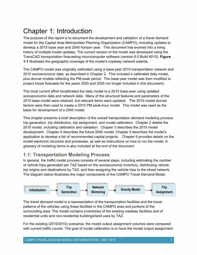
1.1: Transportation Modeling Process In general, the traffic model process consists of several steps, including estimating the number of vehicle trips generated per TAZ based on the socioeconomic inventory, distributing vehicle trip origins and destinations by TAZ, and then assigning the vehicle trips to the street network. The diagram below illustrates the major components of the CAMPO Travel Demand Model.
The travel demand model is a representation of the transportation facilities and the travel patterns of the vehicles using these facilities in the CAMPO area and portions of the surrounding area. The model contains inventories of the existing roadway facilities and of residential units and non-residential buildings/land-uses by TAZ.
For the existing (2010/2015) scenarios, the model output assignment volumes were compared with current traffic counts. The goal of model calibration is to have the model output assignment
Initialization Trip
Generation Network
Skimming Gravity Model
Trip Assignment

CAMPO TRAVEL DEMAND MODEL DOCUMENTATION – MAY 2019 2
volumes match the traffic counts as closely as possible. The model is deemed calibrated when these two sets of traffic volumes match within acceptable ranges of error. The model can then be used to test alternative scenarios with a level of confidence. These scenarios may encompass changes in housing unit counts, employment, travel behavior patterns, or roadway capacity/characteristics.
For future scenarios, a transportation planner or engineer can use the travel demand model to project future traffic volumes. These future-year volumes can aid in making planning and project programming decisions.
Figure 1-1: Model Extents
63
50
63
179
54
54

CAMPO TRAVEL DEMAND MODEL DOCUMENTATION – MAY 2019 3
The model steps are briefly described below.
Trip Generation The number of trips generated by a TAZ is a function of the land use and socioeconomic characteristics. Residential land uses are generally referred to as "producers" of trips; non-residential land uses are generally referred to as "attractors" of trips. Residential trip production is generally a function of the number of dwelling units and other demographic variables. Non-residential trip attraction is generally a function of employment.
The final product of the trip generation step is a table summarizing the total number of person-trips produced by, and attracted to, each TAZ. These trips are categorized by trip purpose (e.g., home-based work). A trip is defined as a one-way movement between two points.
Trip Distribution The purpose of trip distribution is to produce a trip table of the estimated number of trips from each TAZ to every other TAZ within the model. The final product of the trip distribution phase is a person-trip matrix specifying the number of person-trips that travel between each pair of TAZs. Trip matrices are estimated for each of the five trip purposes. The matrices identify the production TAZ and the attraction TAZ for each trip, but they do not indicate the direction of travel. The distribution of trips between TAZs (for example, zone I and zone J) is a function of the “Gravity Model” that includes the following variables:
The number of trips produced by zone I The number of trips attracted by zone J The travel time between zone I and zone J The magnitude of the total "attractiveness" of all the zones in the network
The number of trips traveling between zone I and zone J is directly proportional to the total number of trips produced by zone I and the total number of trips attracted by zone J. For example, the total number of trips traveling between zones I and J increase as the number of residential trips increases in zone I. Further, the number of trips between zones I and J are inversely proportional to the travel time between the two zones. (The number of trips decreases as travel time increases.)
Traffic Assignment The traffic assignment phase converts the person-trip production and attraction matrices to vehicle-trip origin and destination (O-D) matrices based on vehicle occupancy information and direction of travel data. Directionality information is critical for peak-hour modeling. The traffic assignment then allocates each trip to one specific network route based on the travel “costs” (a function of travel time) between the various zones. The traffic assignment process includes the following:
Computation of the minimum-cost paths between the TAZs based on free-flow link speeds (i.e., posted speed limits)
Initial assignment of the trips to the links which lie on the minimum-cost paths between the TAZs
CAMPO TRAVEL DEMAND MODEL DOCUMENTATION – MAY 2019 4
Computation of volume-to-capacity (v/c) ratios on the links after initial assignment
Computation of travel costs on the links as a function of the v/c ratio
Reiteration of the assignment process until the model assignment reaches equilibrium where no traffic can be shifted without increasing the overall network travel cost
The final product of the traffic assignment process is a “loaded” network with traffic volumes on each link. Model Calibration Calibration involves adjusting model parameters and attributes to the point where modeled existing conditions match actual existing conditions within allowable tolerances. The travel demand model is calibrated using the base-year transportation network, socioeconomic estimates, and traffic counts. The calibration process involves reviewing the assumptions and steps used to construct the model. The results of each model step are reviewed and adjustments made to achieve the desired results. During the distribution step, the parameters of the gravity model are examined. During the assignment step, the assumptions for link speeds, capacities, and delay parameters are studied. Any modifications made to the CAMPO model parameters have been justified using available travel pattern data, local knowledge of travel conditions, or empirical modeling knowledge. The model calibration includes a review of several performance measures such as percent assignment error, root mean square error (RMSE), and screenline analysis.

CAMPO TRAVEL DEMAND MODEL DOCUMENTATION – MAY 2019 5
Chapter 2: 2010 Model
The primary goal of the 2010 base-year model was to replicate daily travel patterns on the roadway network in the CAMPO region for a typical weekday in 2010. An accurate base year model, with its equations and parameters, can then be used to model future-year conditions by changing the land use and network input data. Developing an effective base-year model requires gathering, coding, and using a wide range of transportation-related data to create a "snapshot" in time.
2.1: Roadway Network The initial step in the travel demand modeling process was the development of the geographical roadway network comprised of nodes and links. A node is an intersection of two or more links such as an intersection of two street segments. A network link is a street segment between two nodes (A node and B node). CAMPO provided a preliminary GIS-based roadway network file with necessary characteristics (i.e. street names, lanes, speeds, one-way links, etc) as well as additional non-model attribute data. In addition to converting the GIS file to a TransCAD file, refinements to the roadway network (modification and densification) were made in coordination with CAMPO staff.
Some roadways or roadway segments that may not carry substantial volumes may still be important to the model in other ways:
They may alleviate traffic on other roadways by providing alternate routes or additional loading points for trips entering/exiting a Traffic Analysis Zone (TAZ).
They also may provide a route through a TAZ (or TAZs) where a less dense model network might not. Most small neighborhood roads within a TAZ are modeled via centroid
Table 2-1: TransCAD Link Attributes (2010 Model)
Attribute Description
ID Link ID Number
Length Length (miles)
Dir One-way (1, -1) or Two-way (0)
Name Street Name
FunClass Roadway Functional Classification Number 1. Freeway 5. Collector 2. Expressway* 6. Local Residential 3. Primary Arterial 7. Local Ramp 4. Secondary Arterial* 8. System Ramp *Reserved, but currently unused by model
MedianType 1 = Undivided 2 = Undivided with turn lanes at intersections 3 = Through with left turn lanes (TWLTL) 4 = Raised Median – No turn lanes 5 = Raised Median – With turn lanes
AB_Lane BA_Lane
Number of Lanes
AB_Speed BA_Speed
Posted Speed (mph)
SlopePercent
Percent Slope / Grade 0 = 0 to 2.99% 3 = greater or equal to 3%
ADT Estimated Base Year Daily Traffic Count
LaneCap_D Directional Daily Lane Capacity (see Table 2)
AB_Cap_D BA_Cap_D
Directional Daily Roadway Capacity
Alpha Volume Delay Function parameter
Beta Volume Delay Function parameter
The base-year model has been updated to the year 2015, as described in Chapter 3. This chapter is included for historical reference, and also because many of the components of the 2015 model were originally developed in the 2010 model – and thus Chapter 2 is often referenced by Chapter 3.
CAMPO TRAVEL DEMAND MODEL DOCUMENTATION – MAY 2019 6
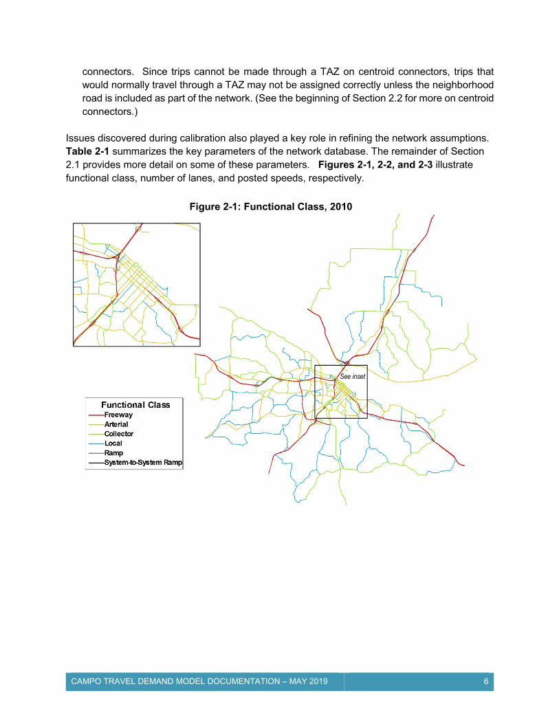
connectors. Since trips cannot be made through a TAZ on centroid connectors, trips that would normally travel through a TAZ may not be assigned correctly unless the neighborhood road is included as part of the network. (See the beginning of Section 2.2 for more on centroid connectors.)
Issues discovered during calibration also played a key role in refining the network assumptions. Table 2-1 summarizes the key parameters of the network database. The remainder of Section 2.1 provides more detail on some of these parameters. Figures 2-1, 2-2, and 2-3 illustrate functional class, number of lanes, and posted speeds, respectively.
Downtown Inset Map
See inset
Figure 2-1: Functional Class, 2010

CAMPO TRAVEL DEMAND MODEL DOCUMENTATION – MAY 2019 7
See inset
Downtown Inset Map
Downtown Inset Map
See inset
Note: Divided highways and some four-lane arterials were coded with two links, so they appear as two-lane highways in each direction of travel.
Figure 2-3: Posted Speeds, 2010
Figure 2-2: Lanes, 2010

CAMPO TRAVEL DEMAND MODEL DOCUMENTATION – MAY 2019 8
Roadway Link Capacity (2010) The model computes link capacities at run time. Capacities are initially based on functional class and number of lanes, adjusted based on directionality, median type, and roadway slope. Capacity is expressed in terms of vehicles per day for each link by direction. Link capacities are not directly entered by the user, but are important parameters in model operation and network analysis.
In the context of model operation, the capacities are used in conjunction with link speeds, link lengths, and link delay functions to derive a realistic travel speed to be used in the trip distribution and assignment stages. In the context of network analysis, the capacities are used to identify deficiencies and recommend improvements. In both cases, it is desired that the capacities used in the model be as accurate and realistic as possible. However, it is also important to point out that these are planning-level calculations appropriate for modeling and long-range planning, as opposed to design-level capacities or calculations.
Table 2-2 includes the base directional capacities used for the 2010 model. These capacities are based on published sources and experience in developing travel demand model planning capacities. Functional classes 2 and 4 are not utilized in the model at present, but they could be used during future model updates.
To calculate a directional link capacity, the base values in Table 2-2 are multiplied by the number of lanes in a specific direction and then multiplied by factors associated with the median type, slope percent, and one-way link adjustment factors, as appropriate.
The median type adjustment factor accounts for capacity changes due to median type and total number of lanes, particularly non-freeway and non-expressway links. A roadway without turn lanes is considered to have less capacity than the same type of roadway with turn lanes. A lack of a median also decreases the capacity of a roadway in comparison to the base capacity. These capacity increases and decreases are also based on guidance from the Florida Department of Transportation (FDOT) Generalized Service Volume Tables from 2010, a widely used transportation planning resource. Figure 2-4 illustrates median types as coded in the 2010 model.
Table 2-2: Daily Link Capacities, 2010 (per-lane) Base Directional Daily Lane Capacity
Roadway Classification
1. Freeway 20,000
2. Expressway* --
3. Primary Arterial 9,000
4. Secondary Arterial* --
5. Collector 7,500
6. Local 6,000
7. Ramp 12,000
8. System-to-system Ramp 40,000
*Reserved, but currently unused by model Source: FDOT, other Missouri models, HDR
Median Type Adjustment Factors, 2010 (multiplied by base capacity for two-way
links of functional class 3+) Total Lanes
Median Type 1-2 3+
1 Undivided 0.67 0.75
2 Undivided with Turn Lanes 0.87 0.95
3 Two-Way-Left-Turn-Lane 0.9 0.98
4 Raised Median no Turn Lanes 0.72 0.8
5 Raised Median with Turn Lanes 0.92 1
One-Way Link Adjustment Factor,
2010
Multiply base capacity
by 1.2 for one-way links
of functional class 3+

CAMPO TRAVEL DEMAND MODEL DOCUMENTATION – MAY 2019 9
The one-way link adjustment factor of 1.2 applies to one-way links that are not freeways or ramps. This 20-percent capacity increase is derived from the FDOT capacity tables. One-way links are considered to have relatively more capacity associated with a lack of opposing traffic. Figure 2-5 illustrates one-way (non-freeway, non-ramp) links as coded in the 2010 model.
For all two-lane collectors and local links with slope percents defined as 3% or greater, the capacity is reduced by 5%. This applies to one-way links with between one and three lanes as well.
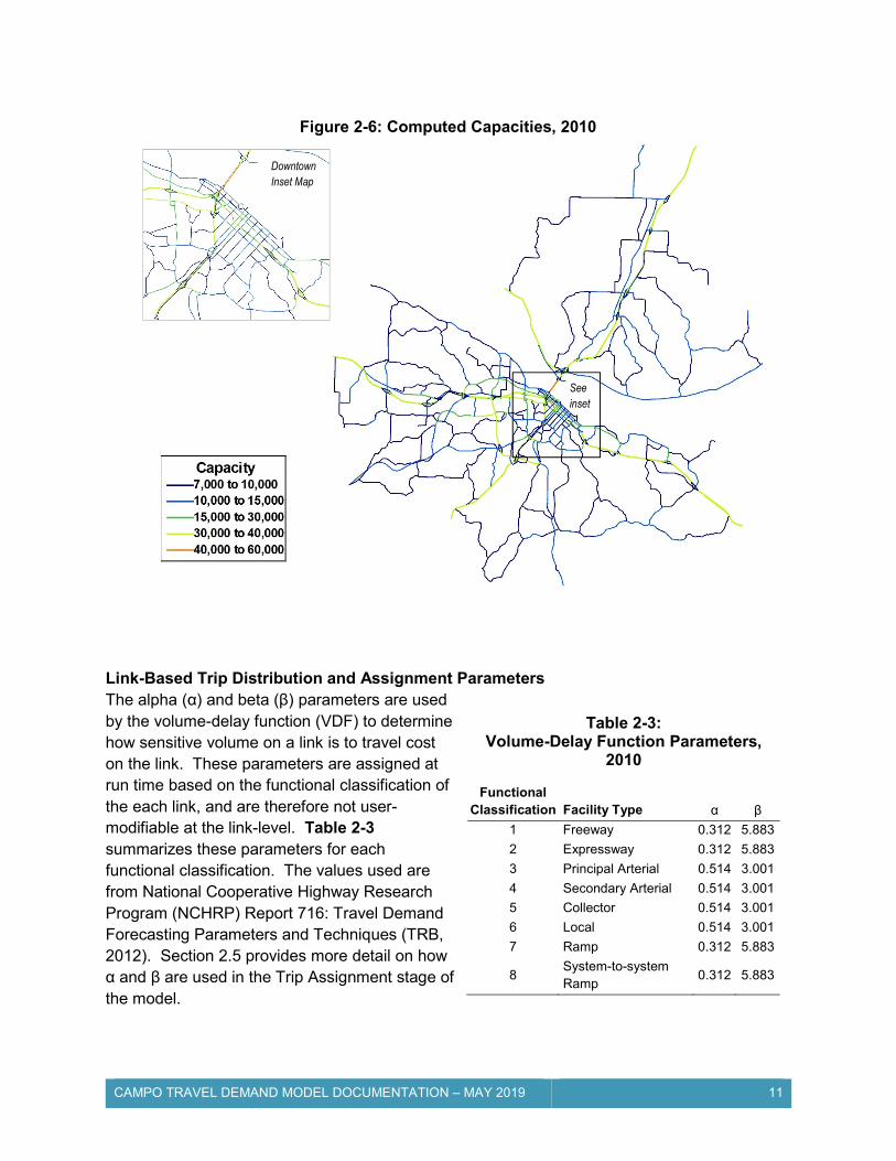
Based on the calculations described above, Figure 2-6 illustrates the capacities computed for the 2010 Daily Model.

CAMPO TRAVEL DEMAND MODEL DOCUMENTATION – MAY 2019 10
Figure 2-4: Median Type, 2010
Figure 2-5: One-Way Links, 2010
See inset
Downtown Inset Map
Downtown Inset Map
See inset
CAMPO TRAVEL DEMAND MODEL DOCUMENTATION – MAY 2019 11
Link-Based Trip Distribution and Assignment Parameters The alpha (α) and beta (β) parameters are used by the volume-delay function (VDF) to determine how sensitive volume on a link is to travel cost on the link. These parameters are assigned at run time based on the functional classification of the each link, and are therefore not user-modifiable at the link-level. Table 2-3 summarizes these parameters for each functional classification. The values used are from National Cooperative Highway Research Program (NCHRP) Report 716: Travel Demand Forecasting Parameters and Techniques (TRB, 2012). Section 2.5 provides more detail on how α and β are used in the Trip Assignment stage of the model.
Table 2-3: Volume-Delay Function Parameters,
2010
Functional Classification Facility Type α β
1 Freeway 0.312 5.883
2 Expressway 0.312 5.883
3 Principal Arterial 0.514 3.001
4 Secondary Arterial 0.514 3.001
5 Collector 0.514 3.001
6 Local 0.514 3.001
7 Ramp 0.312 5.883
8 System-to-system Ramp
0.312 5.883
Figure 2-6: Computed Capacities, 2010
Downtown Inset Map
See inset

CAMPO TRAVEL DEMAND MODEL DOCUMENTATION – MAY 2019 12
Turn Penalties (2010) In order to accurately reflect travel behavior in the CAMPO area, both global and link-specific turn penalties were used in the model. Turn penalties add time (delay) to specific turn movements within the roadway network. This in turn can make particular routes less attractive relative to other travel routes. Penalties can even be used to prohibit certain movements. Figure 2-7 summarizes the turn penalties used in the model, which fall into two categories (global and link-specific) as described below.
Global - Turn penalties were applied to all left- and right-turn movements based on the functional classification of the street being turned onto and the street being turned from. A matrix of global turn penalties is shown in Figure 2-7. U-turns were prohibited throughout the model network, to prevent unrealistic vehicle assignments in areas with other turn penalties, especially near interchanges.
Link-Specific - These penalties were assigned to locations where traffic is physically or
legally prohibited from making the restricted movement. In locations where one-way links are coded within the model, TransCAD automatically prohibits travel in the opposite direction. Therefore, turn penalties are not required at these locations. The link-specific turn penalties defined for use in the daily model are shown in red in Figure 2-7.
Other Adjustments (2010) Terminal Times - To account for the parking and walking time at either end of a trip,
terminal time was added to all trips. One minute was added at either end of all trips, except for though trips in the downtown core, which had 1.5 minutes added.
Speed Reductions - Due to noted over-assignment of volume on the freeway facilities
(Functional Class 1), it was necessary to apply a universal speed reduction factor to those facilities. This factor allows the model to account for the observed travel behavior in the Jefferson City area, which includes drivers selecting routes based on distance, local preference, comfort, and past use; not just travel time.
Link Time - A parameter was included in the network to add time to specific links that are
over-assigned due to factors not captured by the other model elements. However, this feature was not needed to calibrate the daily model. It is available if needed in future model applications or updates/adjustments.

CAMPO TRAVEL DEMAND MODEL DOCUMENTATION – MAY 2019 13
Global
Fre
eway
Art
eri
al
Co
llect
or
Lo
cal
Ra
mp
Sys
tem
-to
-S
yste
m R
amp
Ce
ntr
oid
C
on
ne
cto
r
Fre
eway
Art
eri
al
Co
llect
or
Lo
cal
Ra
mp
Sys
tem
-to
-S
yste
m R
amp
Ce
ntr
oid
C
on
ne
cto
r
Freeway 0.12 0.30 0.30 0.30 0.04 0.04 0.30 0.12 0.30 0.30 0.30 0.04 0.04 0.30
Arterial 0.30 0.12 0.10 0.08 0.10 0.10 0.06 0.30 0.12 0.10 0.08 0.10 0.10 0.06
Collector 0.30 0.12 0.04 0.02 0.08 0.08 0.02 0.30 0.12 0.04 0.02 0.08 0.08 0.02
Local 0.30 0.12 0.04 0.02 0.08 0.08 0.02 0.30 0.12 0.04 0.02 0.08 0.08 0.02
Ramp 0.02 0.10 0.08 0.08 0.08 0.08 0.06 0.02 0.10 0.08 0.08 0.08 0.08 0.06
System-to-System Ramp
0.02 0.10 0.08 0.08 0.08 0.08 0.06
0.02 0.10 0.08 0.08 0.08 0.08 0.06
Centroid Connector 0.30 0.06 0.02 0.02 0.06 0.06 0.02 0.30 0.06 0.02 0.02 0.06 0.06 0.02
LEFT TURNS RIGHT TURNS
Figure 2-7: Turn Penalties, 2010
Link-Specific
Downtown Inset Map
See inset

CAMPO TRAVEL DEMAND MODEL DOCUMENTATION – MAY 2019 14
2.2: Land Use/Socioeconomic Data Traffic Analysis Zone (TAZ) Structures (2010) Land-use and socioeconomic data provide the foundation for the Trip Generation stage of the model.
Land use was developed for different categories and allocated to TAZs. TAZs are generally bounded by some combination of roadways, geographic features (river, railroad, steep terrain), and municipal boundaries. They also generally follow Census 2010 block boundaries.
The TAZ polygon layer contains all relevant TAZ-related attributes. The network feature that ties the TAZ and the network layers to each other is the centroid, a special network node at which all trips within a TAZ are assumed to begin and end for modeling purposes. Each TAZ centroid is connected to at least one roadway link by centroid connectors. Centroid connectors are proxies for local streets within the TAZ that connect to the model roadway network.
The model also includes a special type of TAZ known as an external station. Because the model’s land-use data cannot stretch on endlessly, external stations are used to represent the physical locations at which vehicles can enter or exit the model. Rather than land-use and socioeconomic data, these externals are coded with trip ends broken out by purpose based on available count and survey data.
Figure 2-8 depicts the TAZ structure for the 2010 model. There are 414 TAZs in total: 400 internal TAZs and 14 external stations. The external stations are numbered from 401 through 414. Note that 81 of the internal zones were created and reserved for future use to simplify coding when needed.
The TAZs developed for the 2010 model were created using the potential new urban area boundaries supplied by CAMPO. The approximated urban area includes New Bloomfield to the north of Jefferson City as well as Wardsville to the south. The zone structure was created based on aggregating the 2010 Census blocks using modeling judgment. In a few instances, it was necessary to split Census blocks, because the block geography did not adequately capture how the land use was divided in an area and/or how the land use was distributed within the area via the network.

CAMPO TRAVEL DEMAND MODEL DOCUMENTATION – MAY 2019 15
Figure 2-8: TAZ Structure, 2010
External TAZs
Internal TAZs
Extra TAZs Extra TAZs
Downtown Inset Map
See inset

CAMPO TRAVEL DEMAND MODEL DOCUMENTATION – MAY 2019 16
Household Source Data As described in more detail in Section 2.3, the model’s trip productions are based on data regarding population and household data (the latter including household size and auto ownership). The 2010 population and households entered into the model were derived from the 2010 Census Block data, aggregated into the model TAZs.
Section 2.3 also describes the use of auto-ownership data in the cross-classification methodology for determining trip productions. To derive a generalized model-wide relationship between household size and auto ownership, 2010 Census information was used (at the tract level, for tracts completely or partially in the model area) For each of 18 tracts, auto ownership data was available for each household size increment, and these values were averaged over the 18 tracts to yield reasonable model-wide estimates. Figure 2-9 illustrates the individual tract data and includes a map illustrating the tracts that were selected for this analysis. The final correlation is included in Section 2.3.
Figure 2-9: 2010 Census Data Underlying Household Size / Auto Ownership Correlation
HH Size = 1 HH Size = 2 HH Size = 3 HH Size = 4
Auto Ownership Profiles for 18 Census Tracts in CAMPO Area Autos per HH
18 tracts 18 tracts 18 tracts 18 tracts
18 Census Tracts
Derived Correlation

CAMPO TRAVEL DEMAND MODEL DOCUMENTATION – MAY 2019 17
Employment Source Data As described in more detail in Section 2.3, the model’s trip attractions are based on employment totals in various categories. The US Bureau of the Census Longitudinal Employer-Household Dynamics (LEHD) data was used to estimate the 2010 employment totals for the model. This data provides employment estimates at the Census block level. The employment is categorized using the two-digit North American Industry Classification System (NAICS) codes. The employment data is derived from state and federal unemployment insurance system data. The two-digit NAICS codes and the assumed relationships provided in Table 2-4 were used to consolidate the 20 employment categories into the eight basic CAMPO model land-use categories.
The LEHD data was cross-checked against, and in many cases modified based upon, several other employment sources including ReferenceUSA, Dun & Bradstreet, other CAMPO-provided employment data, internet searches, and aerial photography.
The retail employees were also divided into standard and high-trip-generating retail categories. This was done as part of the calibration effort to better reflect trip-making in some of the high-intensity retail areas.
Total employees within each of the model categories are shown in Table 2-5. As the table indicates, just over 50,000 employees are included in the 2010 model.
Table 2-4: LEHD Conversion to CAMPO Land Use Categories
NAICS Code Description
Model Category
11 Agriculture, Forestry, Fishing and Hunting
Other
21 Mining, Quarrying, and Oil and Gas Extraction
Other
22 Utilities Other
23 Construction Other
31-33 Manufacturing Industrial
42 Wholesale Trade Warehouse
44-45 Retail Trade Retail
48-49 Transportation and Warehousing Warehouse
51 Information Office/Service
52 Finance and Insurance Office/Service
53 Real Estate and Rental and Leasing Office/Service
54 Professional, Scientific, and Technical Services
Office/Service
55 Management of Companies and Enterprises
Office/Service
56 Administrative and Support and Waste Management and Remediation Services
Office/Service
61 Educational Services Education
62 Health Care and Social Assistance Medical
71 Arts, Entertainment, and Recreation Entertain/Rec
72 Accommodation and Food Services Retail
81 Other Services (except Public Administration)
Office/Service
92 Public Administration Office/Service
Table 2-5: Land Use by Type, 2010
Category Employees Retail 4,670 Retail (High) 3,275 Office/Service 24,414 Education 2,678 Medical 4,905 Industrial 4,091 Warehouse 1,869 Entertain/Recr 578 Other 3,533 Total 50,014

CAMPO TRAVEL DEMAND MODEL DOCUMENTATION – MAY 2019 18
2.3: Trip Generation Trip generation has two primary components: trip productions and trip attractions. The CAMPO model’s approach to each is described below.
Trip Productions The CAMPO model generates trip productions for five different purposes:
Home-Based Work (HBW): Trips that have one trip end at home and one trip end at work.
Home-Based School (HBSCH): Trips that have one end at home and the other at a school (elementary through university).
Home-Based Shopping (HBSHOP): Trips that have one end at home and one end at a retail-type shopping location.
Home-Based Other (HBO): All other home-based trips.
Non-Home-Based (NHB): Trips that do not begin or end at home.
Note that for all home-based trips, the home end is considered the production end and the non-home end is considered the attraction end, regardless of the direction of the trip. (In/Out percentages are used to obtain the correct directionality in the peak-hour modeling.)
The trip-production component of the model uses a cross-classification methodology that looks at both household size and auto ownership. Table 2-6 includes the trip production rates for the five trip purposes for each auto-ownership/ household-size combination. Figures 2-10, 2-11, and 2-12 show the per-TAZ values for number of households, average household size, and average auto-ownership, respectively.
The trip production rates employed in the CAMPO travel demand model are based on the rates presented in NCHRP 716. During the calibration process, it was hypothesized that the CAMPO region generates trips at a slightly higher rate than the average for the nation. This proposal was based in part on the low forecasted traffic volumes on the regional roadways using the national average trip production rates (in conjunction with other national average parameters such as trip lengths). Therefore, the following factors were applied to the NCHRP 716 rates: HBW - 1.15; HBSCH - 1.4; HBSHOP – 1.15 HBO – 1.05; NHB – 1.1.
Table 2-6: Trip Production Rates (2010)
Autos per Household
Persons per
Household
Home-Based Non-Home-Based TOTAL Work School Shop Other
0
1 0.23 0.01 0.41 1.1 0.77 2.52 2 0.81 0.14 1.06 2.71 1.87 6.59
3 1.15 1.12 1.57 3.82 2.2 9.86
4 1.15 2.10 1.85 4.51 4.07 13.68
5+ 1.15 2.24 2.2 7.02 4.29 16.9
1
1 0.69 0.01 0.67 1.39 1.54 4.3
2 0.92 0.14 1.31 2.8 2.53 7.7
3 1.38 1.12 2.17 3.9 3.85 12.42
4 1.96 2.24 2.23 5.42 4.29 16.14
5+ 1.73 3.36 2.26 7.6 4.29 19.24
2
1 0.81 0.01 0.64 1.93 1.76 5.15
2 1.5 0.14 1.35 2.97 2.86 8.82
3 2.3 1.12 2.06 4.11 4.29 13.88
4 2.3 2.38 2.14 7.7 6.05 20.57
5+ 2.65 3.64 2.65 9.23 6.16 24.33
3+
1 1.04 0.01 0.64 2.04 1.76 5.49
2 1.61 0.14 1.38 2.94 2.97 9.04
3 2.99 1.12 2.04 4.86 4.95 15.96
4 3.34 2.52 2.12 7.72 6.38 22.08
5+ 3.80 3.78 3.08 10 7.81 28.47

CAMPO TRAVEL DEMAND MODEL DOCUMENTATION – MAY 2019 19
Figure 2-10: Trip Production Variables – Households Per TAZ (2010)

CAMPO TRAVEL DEMAND MODEL DOCUMENTATION – MAY 2019 20
Figure 2-11: Trip Production Variables – Average Household Size Per TAZ (2010)

CAMPO TRAVEL DEMAND MODEL DOCUMENTATION – MAY 2019 21
Figure 2-12: Trip Production Variables – Average Auto Ownership Per TAZ (2010)

CAMPO TRAVEL DEMAND MODEL DOCUMENTATION – MAY 2019 22
Trip Attractions Trip attractions are generally places of employment. Attractions are estimated based on the trip-generation characteristics of the land-uses within the TAZs, and (like productions) are broken out by trip purpose. The trip attraction rates employed in the CAMPO model were primarily derived from the rates provided in NCHRP 716 as well as other travel demand models for smaller urban areas. They were adjusted during the calibration phase to reflect local trip-making characteristics and to more closely match the calibrated trip productions. The final trip attraction rates used in the model compare well with, but are slightly higher than, the NCHRP 716 rates. Table 2-7 summarizes the trip attraction rates by land-use category, broken out by trip purpose.
Figures 2-13, 2-14, 2-15, and 2-16 illustrate the per-TAZ values for many of the variables listed in Table 2-7.
Table 2-7: Trip Attraction Rates (2010)
Trip Purpose
Total Land Use HBW HBSCH HBSHOP HBO NHB
HH 0 0 0 1.309 0.855 2.164
Retail 1.311 0 7.4 0.99 5.238 14.939
Office/Service 1.311 0 0 2.5 0.981 4.792
Education 1.311 10.0 0 0 1.5 12.811
Medical 1.311 0 0 3.751 0.981 6.043
Industrial 1.311 0 0 0.517 0.432 2.26
Warehouse 1.311 0 0 0.517 0.432 2.26
Entertain/Recr 1.311 0 0 0.517 0.432 2.26
Other 1.311 0 0 0.517 0.432 2.26
Retail - High Density
1.311 0 7.8 1.045 5.328 15.484

CAMPO TRAVEL DEMAND MODEL DOCUMENTATION – MAY 2019 23
Figure 2-13: Trip Attraction Variables – Retail Employees per TAZ (2010)

CAMPO TRAVEL DEMAND MODEL DOCUMENTATION – MAY 2019 24
Figure 2-14: Trip Attraction Variables – Office/Service Employees per TAZ (2010)

CAMPO TRAVEL DEMAND MODEL DOCUMENTATION – MAY 2019 25
Figure 2-15: Trip Attraction Variables – Industrial/Warehouse Employees per TAZ (2010)

CAMPO TRAVEL DEMAND MODEL DOCUMENTATION – MAY 2019 26
Figure 2-16: Trip Attraction Variables – All Other Employee Categories per TAZ (2010)

CAMPO TRAVEL DEMAND MODEL DOCUMENTATION – MAY 2019 27
External Stations (2010) Once the internal trip generation estimates were complete, it was necessary to prepare external station “trip generation” estimates. As mentioned previously, external stations are used to represent the physical locations at which vehicles can enter or leave the model. Rather than land-use and socioeconomic data, these externals are coded with trip ends broken out by purpose based on available count and survey data.
Figure 2-17 illustrates the counts at the model’s 14 external stations.
Figure 2-17: External Station Volumes, 2010 Daily
Rte 179 565 vpd
US-63 18,359 vpd
Rte Y 744 vpd
Rte J 428 vpd
US-54 N 10,780 vpd
Rte. BB 280 vpd
Rte. 94 2,162 vpd
US-50 E 14,774 vpd
Rte W 1,488 vpd
Rte B/E 2,800 vpd
US-54 S 18,918 vpd
Rte C 4,250 vpd
Meadows Ford 1,046 vpd
US-50 W 9,368 vpd
CAMPO TRAVEL DEMAND MODEL DOCUMENTATION – MAY 2019 28
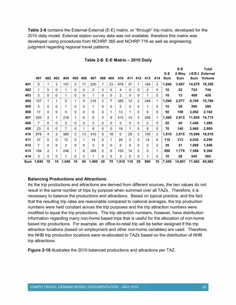
Table 2-8 contains the External-External (E-E) matrix, or “through” trip matrix, developed for the 2010 daily model. External station survey data was not available, therefore this matrix was developed using procedures from NCHRP 365 and NCHRP 716 as well as engineering judgment regarding regional travel patterns.
Balancing Productions and Attractions As the trip productions and attractions are derived from different sources, the two values do not result in the same number of trips by purpose when summed over all TAZs. Therefore, it is necessary to balance the productions and attractions. Based on typical practice, and the fact that the resulting trip rates are reasonable compared to national averages, the trip production numbers were held constant across the trip purposes and the trip attraction numbers were modified to equal the trip productions. The trip attraction numbers, however, have distribution information regarding many non-home based trips that is useful for the allocation of non-home based trip productions. For example, an office-to-retail trip will be better assigned if the trip attraction locations (based on employment and other non-home variables) are used. Therefore, the NHB trip production locations were re-allocated to TAZs based on the distribution of NHB trip attractions.
Figure 2-18 illustrates the 2010 balanced productions and attractions per TAZ.
Table 2-8: E-E Matrix – 2010 Daily
401 402 403 404 405 406 407 408 409 410 411 412 413 414 E-E Sum
E-E 2-Way Sum
I-E/E-I Sum
Total External Volume
401 0 1 3 157 3 17 520 7 23 878 37 7 184 3 1,840 3,687 14,679 18,359
402 1 0 0 1 0 0 2 0 0 4 0 0 2 0 10 22 724 744
403 3 0 0 1 0 0 1 0 0 2 0 0 1 0 10 13 408 428
404 157 1 1 0 1 5 216 2 7 385 12 2 248 1 1,040 2,077 8,700 10,780
405 3 0 0 1 0 0 1 0 0 2 0 0 1 0 10 28 260 280
406 17 0 0 5 0 0 6 0 1 13 1 0 6 0 50 108 2,062 2,162
407 520 2 1 216 1 6 0 3 9 415 14 3 268 1 1,460 2,913 11,854 14,774
408 7 0 0 2 0 0 3 0 0 5 0 0 2 0 20 45 1,448 1,488
409 23 0 0 7 0 1 9 0 0 18 1 0 9 0 70 140 2,660 2,800
410 878 4 2 385 2 13 415 5 18 0 29 5 150 3 1,910 3,815 15,098 18,918
411 37 0 0 12 0 1 14 0 1 29 0 0 14 0 110 213 4,030 4,250
412 7 0 0 2 0 0 3 0 0 5 0 0 2 0 20 31 1,006 1,046
413 184 2 1 248 1 6 268 2 9 150 14 2 0 1 890 1,779 7,588 9,368
414 3 0 0 1 0 0 1 0 0 3 0 0 1 0 10 28 545 565
Sum 1,840 10 10 1,040 10 50 1,460 20 70 1,910 110 20 890 10 7,450 14,901 71,062 85,962

CAMPO TRAVEL DEMAND MODEL DOCUMENTATION – MAY 2019 29
Figure 2-18: Productions and Attractions per TAZ, 2010

CAMPO TRAVEL DEMAND MODEL DOCUMENTATION – MAY 2019 30
2.4: Trip Distribution The purpose of the trip distribution step is to produce a trip table of the estimated number of trips from each TAZ to every other TAZ within the study area. The person-trip distribution for the CAMPO model uses TransCAD’s Gravity Model routines. The Gravity Model assumes that the number of person-trips between two zones is (1) directly proportional to the person-trips produced and attracted to both zones, and (2) inversely proportional to the travel time between the zones.
For this model, the Gravity Model uses the gamma function shown at the bottom of Table 2-9 as the primary travel-time-related impedance input. The gamma function calculates friction factors F(tij) for each zone pair based on the travel time (tij) between zones and three parameters (a, b, and c). Friction factors express the effect travel time has on the number of trips traveling between two zones. The calculation of friction factors differs by trip type reflecting the fact that some types of trips are more or less sensitive to trip length.
The parameters a, b, and c were initially derived from the “Small MPO” values in NCHRP Report 716. However, these parameters can vary based on model size and local travel behavior. During the model calibration process, these parameters were iteratively adjusted based on model results, including the reported trip lengths, keeping in mind the reasonable ranges described in NHCRP 716 (Travel Demand Forecasting: Parameters and Techniques). The final 2010 values used are displayed in Table 2-9.
The model also makes use of K-factors, which provide additional specific TAZ-to-TAZ attractiveness terms to the gravity equations. K-factors are developed for specific zone pairs and are then used in the Gravity Model equation.
The default K-factor between two zones is 1; however, this can be increased or decreased to adjust the trip distribution to account for factors other than travel-time related impedance. For the CAMPO model K-factors were used during model calibration to improve the trip distribution results for specific trip purposes in specific geographic areas. For example, in order to minimize HBSCH trips from outside of Wardsville to the schools in Wardsville and vice versa, a k-factor of 0.01 was applied to all HBSCH trips traveling between the TAZs roughly representing the Blair Oaks School District and the rest of the model. The K-factors currently in use in the model include:
Table 2-9: Final Friction Factor (Gamma Function) Parameters, 2010
Trip Purpose a b c
HBW 100 0.265 0.038
HBSCH 100 1.340 0.100
HBSR 100 1.017 0.085
HBO 100 1.017 0.065
NHBO 100 0.781 0.125 Gamma Function:
ijtcbijij eattF
Gravity Model Formulation
𝑇 𝑃 ∗𝐴 ∗ 𝑓 𝑡 ∗ 𝐾
∑ 𝐴∈ ∗ 𝑓 𝑡 ∗ 𝐾
Where: 𝑇 = Trips produced in zone i and attracted to zone j;
𝑃 = Production of trips ends for purpose p in zone i;
𝐴 = Attraction of trip ends for purpose p in zone j;
𝑓 𝑡 = Friction factor, a function of the travel
impedance between zone i and zone j, often a specific function of impedance variables (represented compositely as tij) obtained from the model networks; and
𝐾 = Optional adjustment factor, or “K-factor,” used to
account for the effects of variables other than travel impedance on trip distribution.

CAMPO TRAVEL DEMAND MODEL DOCUMENTATION – MAY 2019 31
HBSCH trips to/from TAZs representing Blair Oaks School District and TAZs in the remainder of the model (k-factor 0.01)
HBSCH trips to/from TAZs in the vicinity of Belair elementary school to the TAZ with the school (k-factor greater than 1)
HBSHOP trips within Holt’s Summit and surrounding areas (k-factor 1.5)
Person-trips were distributed separately for the five trip purposes. The number of trips to be assigned was calculated using the base year land-use/socioeconomic data and trip production/attraction rates by trip purpose. Data from the external TAZs were combined with the internal TAZ trips to create the total productions and attractions for the model. The productions and attractions were balanced to ensure that for each production generated by the model, there was an attraction. Table 2-10 summarizes the 2010 person-trips by trip purpose for the complete model area.
Table 2-10: 2010 Person-Trip Summary
Trip Purpose
Person Trips
Percent Trips
HBW 77,729 19%
HBSCH 27,562 7%
HBSHOP 59,453 14%
HBO 133,781 33%
NHB 112,273 27%
Total Trips 410,798 100%
CAMPO TRAVEL DEMAND MODEL DOCUMENTATION – MAY 2019 32
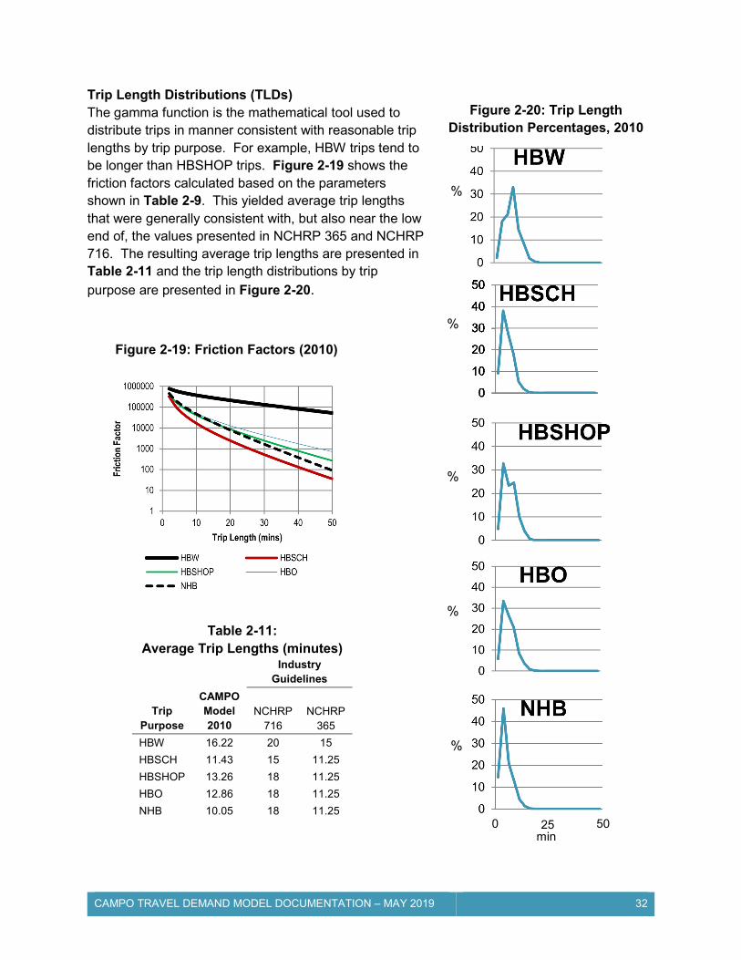
Trip Length Distributions (TLDs) The gamma function is the mathematical tool used to distribute trips in manner consistent with reasonable trip lengths by trip purpose. For example, HBW trips tend to be longer than HBSHOP trips. Figure 2-19 shows the friction factors calculated based on the parameters shown in Table 2-9. This yielded average trip lengths that were generally consistent with, but also near the low end of, the values presented in NCHRP 365 and NCHRP 716. The resulting average trip lengths are presented in Table 2-11 and the trip length distributions by trip
purpose are presented in Figure 2-20.
Figure 2-19: Friction Factors (2010)
Table 2-11: Average Trip Lengths (minutes)
Industry
Guidelines
Trip Purpose
CAMPO Model 2010
NCHRP 716
NCHRP 365
HBW 16.22 20 15
HBSCH 11.43 15 11.25
HBSHOP 13.26 18 11.25
HBO 12.86 18 11.25
NHB 10.05 18 11.25 0 50 25
min
Figure 2-20: Trip Length Distribution Percentages, 2010
%
%
%
%
%

CAMPO TRAVEL DEMAND MODEL DOCUMENTATION – MAY 2019 33
2.5: Daily Trip Assignment The purpose of trip assignment is to assign vehicle trips to specific paths, or routes, in the transportation network. Trip assignment is a function of (1) the shortest travel time (or travel cost function) along paths between zones, and (2) the level of congestion on the links that make up those paths. Vehicle trips for the study area were assigned to the transportation network using the TransCAD Stochastic User Equilibrium (SUE) Assignment Algorithm.
TransCAD provides several traffic assignment methods. The SUE method is based on the commonly used User Equilibrium (UE) assignment method. The UE method uses an iterative process to achieve a convergence in which no travelers can improve their travel times by shifting routes. However, the SUE method produces more realistic assignment results compared to the UE method, because SUE permits use of less attractive as well as the most attractive routes. Less attractive routes will have lower utilization, but will not have zero flow as they do under the UE method.
Input to the SUE assignment is a vehicle origin-destination trip table and the roadway network. Then, the vehicle trip table is assigned to the network based on the modified equilibrium assignment method. The SUE assignment is premised on the assumption that travelers have imperfect information about the network paths and/or vary in their perceptions of network attributes. Equilibrium occurs when a trip in the system cannot be made by an alternate path without increasing the total travel time of all trips in the network. The model convergence is set at 0.005. Thus, when the relative gap between runs reaches this level, the assignment terminates successfully.
The assignment process assigns both internal and external vehicle trips to the network. Internal vehicle trips are those trips with either an origin or a destination inside the study area. The gravity model described in the previous section produces an internal person-trip table which is converted to a vehicle trip table using vehicle occupancies and directionality data. These trips can be classified as either internal-to-internal, internal-to-external, or external-to-internal. However, vehicle trips travelling through the study area must also be assigned to the network. External-to-external trips are through trips - those with both an origin and destination outside of the study area.
The production and attraction (PA) matrix defines the person-trips between zones, but it is based on where trips are produced and attracted, not origins and destinations. For example, a HBW round-trip will have two productions in the home zone and two attractions in the work zone. Therefore, a transformation is required to convert the PA person-trip matrix to an O-D vehicle trip matrix. For a daily run, it is assumed that trips are 50 percent in each direction (round-trips). Therefore, the model transforms productions and attractions into balanced origins and destinations, and a vehicle occupancy is applied to convert person-trips to vehicle trips. Therefore, assuming a vehicle occupancy greater than one person per vehicle, the sum of vehicle trips in the O-D matrix will be less than the sum of person-trips in the PA matrix.
Table 2-12: Vehicle Occupancy by
Purpose – 2010 Daily Trip Purpose
Vehicle Occupancy
HBW 1.10 HBSCH 1.83 HBSHOP 1.44 HBO 1.51 NHB 1.50

CAMPO TRAVEL DEMAND MODEL DOCUMENTATION – MAY 2019 34
Vehicle occupancy rates by trip purpose were based on national statistics and experience with other models. As shown in Table 2-12, the home-based school trips have the highest vehicle occupancy at 1.83 persons per vehicle. The other non-work trip types are in the 1.44 to 1.51-person-per-vehicle range. Home-Based Work trips are lowest, at 1.10 persons per vehicle.
Volume-Delay Function The SUE traffic assignment method uses a volume-delay function to estimate the travel time on any given link for a forecasted volume. In general, travel time on a link increases as the traffic volume on the link approaches capacity. The volume-delay function and parameters selected for a particular model define that relationship.
For the CAMPO model, a volume-delay function was selected that is based on the Bureau of Public Roads (BPR) Function. The basic BPR function has three key input variables: free-flow travel time, volume (flow), and capacity. The remaining inputs are based on the functional class of the roadway. The theory is that congested travel time is a function of free-flow travel and the volume-to-capacity ratio. Table 2-13 includes the BPR function and the parameters used for the CAMPO model.
Figure 2-21 shows the results of the 2010 daily model assignment as a bandwidth plot with heavier volumes shown as heavier lines in the figure. The detailed results of the 2010 daily model are evaluated in the trip calibration section and available for review as GIS files.
Table 2-13: Volume-Delay Function Parameters – 2010 Daily
Functional Classification Facility Type α β
1 Freeway 0.312 5.883
2 Expressway* 0.312 5.883
3 Principal Arterial 0.514 3.001
4 Secondary Arterial*
0.514 3.001
5 Collector 0.514 3.001
6 Local 0.514 3.001
7 Ramp 0.312 5.883
8 System-to-system Ramp
0.312 5.883
* Reserved, but currently unused by model Volume-Delay Function (Congested cost)
i
i
iiii C
xfccc
1
Where:
icc = Congested travel cost (time) on link i
ifc = Free-flow travel cost (time) on link i
ix = Volume (flow) on link i
iC = Capacity of link i
i = Constant
i = Constant

CAMPO TRAVEL DEMAND MODEL DOCUMENTATION – MAY 2019 35
Figure 2-21: Assignment Bandwidth, 2010 Daily

CAMPO TRAVEL DEMAND MODEL DOCUMENTATION – MAY 2019 36
2.6: Peak Hour Trip Assignment Peak-Hour Trip Table The peak hour trip assignment procedure uses the daily model vehicle trip table and then estimates the portion of the daily trips that will occur during the peak hours of interest. The CAMPO model has been developed to provide PM peak hour volume estimates that can be used for future network planning.1 The procedure for deriving the PM peak hour flows from the daily model flows includes the use of a table defining the percent of each trip purpose category (by direction) that is expected in that peak hour. The table also defines any peak hour adjustments to the daily vehicle occupancies. The values used to generate the 2010 PM peak hour volumes are listed in Table 2-14.
The values used in Table 2-14 were originally taken from NCHRP 716, with adjustments made based on a comparison of the model results to actual PM peak hour intersection turning movement counts at key locations (discussed below). These values are used to develop the PM peak-hour vehicle trip table. The summary of the 2010 PM peak hour vehicle trips (excluding external-external trips) by trip purpose is shown in Table 2-15.
PM Peak-Hour Trip Assignment The PM peak-hour vehicle trip table is assigned to the model network in a manner similar to the daily assignment. To accomplish this, additional PM peak-hour model parameters must be populated. First, peak hour link capacities were defined. For the CAMPO model, they were assumed to be 10 percent of the daily capacities. (The peak-hour speeds and number of lanes were assumed to be the same as in the daily model.) Second, it was necessary to develop a PM peak-hour external-external (E-E) matrix. The PM peak hour E-E matrix was assumed to be 10 percent of the daily E-E matrix. With these additional inputs, it was possible to assign the PM trip table to the model network and provide an estimate of PM peak hour flows.
1 The model also includes data for AM peak hour estimates, but those results were not part of the original model scope and were therefore not calibrated.
Table 2-15: 2010 PM Vehicle Trips by Purpose
Trip Purpose Trips
HBW 9,360 HBSCH 890
HBSHOP 4,067
HBO 9,589
NHB 6,729
Total 30,635
Table 2-14: 2010 PM Peak Hour Traffic Flows by Purpose
% of Daily Flow
% Departing
% Returning
Vehicle Occupancy
HBW 12.7% 4% 96% 1.10
HBSCH 5.8% 26% 74% 1.83
HBSHOP 10.5% 43% 57% 1.44
HBO 10.5% 43% 57% 1.51
NHB 8.5% 50% 50% 1.50

CAMPO TRAVEL DEMAND MODEL DOCUMENTATION – MAY 2019 37
Intersection Analysis The eleven locations shown in Figure 2-22 were selected as “critical” intersections. They are located all around the region and were selected together with, and approved by, the CAMPO Board and staff. The PM peak hour assignments were compared to actual traffic counts at these 11 intersections. (Dates of current available traffic counts ranged from 2009 to 2012). Based on that comparison, a variety of network and other model adjustments were made to improve the PM results. These changes had the benefit of improving the daily results as well. Overall, the PM peak hour assignment estimates the intersection approach volumes at an adequate planning level. It does not focus on extreme accuracy at the turning-movement level, but it does appear sufficient for planning-level applications. A post-processing spreadsheet was used to calculate the model over/under–estimation; this spreadsheet was employed for the future year intersection analysis.
Figure 2-22: Study Intersection PM Peak Hour Turning Movement Volumes (Adjusted from Counts), 2010 Daily

CAMPO TRAVEL DEMAND MODEL DOCUMENTATION – MAY 2019 38
To provide a baseline level of service analysis for the 11 key locations, the existing traffic counts were adjusted to an assumed 2010 base year (using a 2% annual growth rate, which, in the case of 2011-2012 counts, meant “backwards factoring”) and entered into the Synchro intersection analysis software. The existing intersection geometry and signal timing/traffic control were also entered. (CAMPO and its member agencies provided nine of the eleven traffic counts as well as all of the necessary signal timing data.) The summary results of the intersection analysis are presented in Table 2-16. From that table, it is clear that all of the signalized intersections, as well as the critical unsignalized movements, currently operate adequately (LOS D or better) at all 11 locations. Two intersections, however, have individual movements that operate at LOS E.
Table 2-16: 2010 PM Peak Hour Intersection Analysis
Sig/Unsig* Delay LOS
1. US-54 SB Ramps & Simon Blvd U 24.6 (SB) C
2. Missouri Blvd EB Ramps & Rte. 179 S 13.9 B
3. US-50 EB/Horner Rd & Truman Blvd S 18.3 B
4. Stadium Blvd & Jefferson St S 34.0 C ǂ
5. Missouri Blvd & Dix Rd S 29.9 C ǂ
6. Missouri Blvd & Beck St S 19.3 B
7. US-54 NB Ramps & Ellis Blvd S 23.8 C
8. US-50/63 EB Ramps & Eastland Dr S 10.7 B
9. Rte. B/W/M** U 16.9 (WB) C
10. US-50/63 WB Ramps & Militia Dr U 8.7 (WB) A
11. US-50 EB/Horner Rd & Big Horn Dr U 15.7 (WB) C
*For unsignalized intersections the delay/LOS reported are for the worst movement at the intersection. **Intersection 9 was analyzed as a two-way stop (east-west stop) because Synchro does not allow analysis of the actual configuration (3-way stop at a 4-way intersection). ǂ One or more movements operate at LOS E.

CAMPO TRAVEL DEMAND MODEL DOCUMENTATION – MAY 2019 39
2.7: Model Calibration/Validation Calibration is an iterative process that involves enhancing or adjusting input data, program coefficients or parameters, and assumptions with the goal of replicating observed travel-related data. Each element of the travel demand model, from the network and land-use assumptions to the traffic assignment parameters, is subject to calibration until the model sufficiently represents the base year conditions. Once the travel demand model is calibrated, the resulting outputs are validated and checked for reasonableness. Preferably, this second step would employ new data sets that differ from those used to originally calibrate the model.
The model calibration should ultimately result in traffic volumes that that are within selected tolerances of actual traffic count data. If the calibrated model can replicate the current traffic data and patterns with sufficient accuracy, and if the results are determined to be valid, then it is ready for use in forecasting. Setting the allowable level of variation is an important step in this process. While differences are unavoidable, the acceptable amount will vary by topic, magnitude, and sample size. Once the model has passed the calibration and validation tests, it would be expected to yield reasonable future-year volumes for transportation planning purposes, given a future year socio-economic / land-use scenario.
Two documents that play a central role in the calibration and validation steps are: NCHRP 716 Travel Demand Forecasting: Parameters and Techniques (Cambridge Systematics, 2012) and Travel Model Validation and Reasonableness Checking Manual 2nd Ed. (Cambridge Systematics, 2010). The remainder of this section will present the model calibration and validation results for each component of the model as well as the model outputs.
Trip Assignment Several tests were applied to make sure that the 2010 model was calibrated and valid (see box at right). The calibration steps check to see if the model sufficiently represents the traffic volumes and patterns, while the validation step then compares the results to other data sets.
Assignment Performance Measures
Percent Assignment Error Root Mean Square Error (RMSE) Coefficient of Determination (R2)
Screenline Analysis

CAMPO TRAVEL DEMAND MODEL DOCUMENTATION – MAY 2019 40
Percent Assignment Error The assigned 2010 daily traffic volumes were compared with the counted daily traffic volumes for individual links. Figure 2-23 shows the predicted vs. actual traffic volumes. The link segments included in the percent error evaluation (i.e. those with counts) are shown in Figure 2-24.
Table 2-17 illustrates the percent assignment error, which is the difference between the assigned traffic volumes and the counted traffic volumes divided by the counted traffic volumes. The report Travel Model Validation and Reasonableness Checking Manual 2nd Ed. presents the error limits used for various models. This analysis employs the values recommended by the FHWA in their 1990 report: Calibration and Adjustment of System Planning Models. The computed percent error is given in Table 2-17 in comparison to the suggested error limits. The percent error of the traffic assignment for the network as a whole was -4.0 percent, and the errors for the individual functional classifications were within acceptable tolerances.
Figure 2-23: 2010 Predicted vs. Actual Volumes
Table 2-17: Percent Assignment Error – 2010 Daily
Percent Error
Functional Class Computed
Suggested Range*
Freeway 2.3% +7%
Primary Arterial -6.8% +10%
Collector -14.0% +25%
Local 0.3% +25%
Overall -4.0% +5%
*Source: Calibration and Adjustment of System Planning Models, Federal Highway Administration, December 1990. The original published values use a slightly different functional classification system:
Freeways ± 7% Principal Arterials ± 10% Minor Arterials ± 15% Collectors ± 25% Frontage Roads ± 25%

CAMPO TRAVEL DEMAND MODEL DOCUMENTATION – MAY 2019 41
Coefficient of Determination Another tool to measure the overall model accuracy is the coefficient of determination or R² (see formula at right). The R², or “goodness of fit”, statistic shows how well the regression line represents the assignment data. The desirable R2 is 0.88 or higher. A value of 1.00 is perfect, but even if traffic counts were compared against themselves, the daily variation would not allow for a regression coefficient of 1.00. The value of 0.926 achieved for the 2010 model illustrates a good fit between the model output and the available counts.
Coefficient of Determination
2
2222
2
iiii
iiii
yynxxn
yxyxnR
Where: x = counts y = model volumes n = number of counts
Figure 2-24: Link Counts for Model Calibration, 2010
Red highlighted links indicate the location of a daily count.

CAMPO TRAVEL DEMAND MODEL DOCUMENTATION – MAY 2019 42
Root Mean Square Error Another measure of the model's ability to assign traffic volumes is the percent RMSE. The RMSE measures the deviation between the assigned traffic volumes and the counted traffic volumes; the calculation is shown at the bottom of Table 2-18. A large percent RMSE indicates a large deviation between the assigned and counted traffic volumes; whereas, a small percent RMSE indicates a small deviation between the assigned and counted traffic volumes. The percent RMSE by facility type for the study area is given in Table 2-18.
Currently, there are no national standards for model verifications of RMSE. However, a number of DOTs have adopted guidelines by link volume group. The Oregon Department of Transportation values are employed here as a guideline by link volume group along with the Montana Department of Transportation recommendation that a model have an overall RMSE of 30 percent or lower. For all volume ranges, the model values are under the recommended guidelines.
Screenline/Cutline Analysis A screenline or cutline is an imaginary line crossing all (screenline) or a portion (cutline) of the model area and intersecting a number of network links. Typically, these lines divide the model area into logical regions or cut across major travel routes. A screenline analysis compares the results of a trip assignment with the traffic counts on network links along that screenline. More precisely, the process compares the sum of daily traffic count volumes across a screenline with the sum of assigned daily traffic volumes across the same screenline.
The average of ratios over all the screenlines can be also used to measure the overall accuracy of the model. The screenlines and associated volumes used in this analysis are included in Table 2-19. The locations of the screenlines are shown graphically in Figure 2-25.
Table 2-18: Percent Root Mean Square Error (RMSE) – 2010 Daily
Volume Ranges RMSE Guidelines*
20,000 to 39,999 7.8% 25.4%
10,000 to 19,999 16.2% 28.3%
5,000 to 9,999 23.9% 43.1%
0 to 4,999 45.2% 115.8%
Overall 26.4% 30.0%
* Source: Minimum Travel Demand Model Calibration and Validation Guidelines for State Of Tennessee
untsNumberofCo
Count
untsNumberofCo
CountModel
RMSEjj
jjj
)1(
)(*100
%
2
Table 2-19: Screenline Analysis – 2010 Daily
Screenline Model
Volume Traffic Count
% Diff FHWA Allowable %
North 18,358 17,052 8% ± 45%
River 54,606 52,757 4% ± 30%
Southeast 57,710 52,445 10% ± 30%
Southwest 98,786 98,398 0% ± 22%
Downtown 214,725 208,758 3% ± 18%
Total 444,185 429,410 3%
Acc
epta
ble
Per
cen
t D
evia
tio
n
Total Screenline Traffic (1000’s)
FHWA Criteria Source: NCHRP 255 p.49 (cited in FHWA, Calibration and Adjustment of System Planning Models, Dec. 1990)

CAMPO TRAVEL DEMAND MODEL DOCUMENTATION – MAY 2019 43
At the conclusion of each model run, assigned volumes from the run were compared against the screenline count data. The resulting deviations were compared against acceptable levels of error as outlined in NCHRP 255 report (illustrated in the graph below Table 2-19).
Figure 2-25: Screenline Locations
North
River
Southeast
Southwest
Downtown
River

CAMPO TRAVEL DEMAND MODEL DOCUMENTATION – MAY 2019 44
Chapter 3: 2015 Base Model Update
3.1: Year 2015 Roadway Network In order to recalibrate to the updated base year of 2015, a number of roadway network modifications were incorporated to reflect actual construction projects that occurred between 2010 and 2015. These projects were provided by CAMPO and are shown in Figure 3-1.
Network attributes, including number of lanes, posted speeds, and median type, were also revisited and updated as necessary for the new 2015 Base.
Roadway Link Capacities Using the updated network links and attributes, link capacities were re-calculated using the same methodology as the 2010 Base, outlined in Chapter 2.
Figure 3-1: Network Modifications - 2015
US 50/63 & Lafayette St Interchange
MO Hwy 179 & Mission Rd Interchange
Creek Trail Drive/ Frog Hollow Road Reconfiguration
Stoneridge Pkwy and Hard Rock Dr Construction

CAMPO TRAVEL DEMAND MODEL DOCUMENTATION – MAY 2019 45
Other Parameters and Adjustments For the 2015 Base model, no new adjustments were made to the volume-delay function parameters, turn penalties, terminal times, speed reductions, or link times. See Chapter 2 for the assumptions and values used in 2010 that were carried forward for 2015.
3.2: Year 2015 Land Use/Socioeconomic Data The TAZ structure created for the 2010 base year was left unaltered for 2015. However, the land use and socioeconomic data was updated within each TAZ to accurately reflect changes that occurred in the CAMPO region between 2010 and 2015.
Household Source Data In the 2010 base model, household data was derived from 2010 Census Block data and aggregated into the model TAZs. For 2015 household data, a different source was used. The Census Bureau conducts an ongoing survey called the American Community Survey (ACS) that provides information on population, housing, income, and auto ownership (among other things) on an annual basis. ACS provides data in one-year, three-year and five-year estimates. The one-year data, while containing the most current data, is the least reliable because it has the smallest sample size. Therefore, for better data accuracy, the CAMPO region data was updated using the five-year (2011-2015) estimates.
Due to the smaller sample size, ACS data is not available at the Block level. The smallest geographic coverage available is at the Block Group level. Therefore, additional steps were taken to help ensure that the data was accurately aggregated to the appropriate model TAZs. This included developing 2015 Block level data by comparing the distribution of 2010 Block data within the 2010 Block Groups, then dividing up the 2015 Block Group data in the same proportions.
Household size and auto ownership data was also derived from the 2015 ACS 5-year estimates. This data was used to update the correlation between household size and auto ownership used in the cross-classification methodology described in Chapter 2.
Employment Source Data As described in Chapter 2, the employment information used in the 2010 Base model was primarily based on the Census Bureau’s 2010 LEHD data set, although it was cross-checked against other data sources and modified from the raw data set.
To update the employment data for the 2015 Base model, LEHD data for 2015 was obtained. The LEHD categories were converted to CAMPO land use categories in the same manner described in Chapter 2, Table 2-4. The 2015 data was also cross-checked against other available sources, including CAMPO-provided data and aerial photography. Adjustments were made as deemed necessary based on these sources. In some cases, the 2010 model data was retained if the 2010 data was significantly modified from LEHD and historic aerial photography did not indicate any
Table 3-1: 2015 Employment by Type
Category Employees
Retail 4,689
Retail (High) 4,165
Office/Service 25,275
Education 2,789
Medical 5,430
Industrial 3,515
Warehouse 1,922
Entertainment/Recreation 557
Other 3,809
Total 52,151

CAMPO TRAVEL DEMAND MODEL DOCUMENTATION – MAY 2019 46
changes between 2010 and 2015. As derived from this update process, total employees within each of the model categories are shown in Table 3-1.
3.3 Trip Generation Trip Productions The 2015 CAMPO Base model continues to use the same five trip purposes as were used in the 2010 Base model:
Home-Based Work (HBW) Home-Based School (HBSCH) Home-Based Shopping (HBSHOP) Home-Based Other (HBO) Non-Home Based (NHB)
As discussed in Chapter 2, the trip production rates employed in the CAMPO 2010 Base model were based on the rates presented in NCHRP 716, but modified to increase trip production during the calibration process. For the 2015 model, the NCHRP rates were adjusted by slightly different factors: HBW – 1.25; HBSCH – 1.4; HBSHOP – 1.2; HBO – 1.2; and NHB – 1.21. The resulting trip production rates for the five trip purposes for each auto-ownership/household size combination is shown in Table 3-2.
Figures 3-2, 3-3, and 3-4 illustrate the updated 2015 trip production variables by TAZ: Total Households, Average Household Size, and Average Auto Ownership, respectively. As shown, values are similar to, but slightly different from, the original 2010 Base model values.
Table 3-2: Trip Production Rates
Autos per
Household
Persons per
Household
Home-Based Non-Home-Based TOTAL Work School Shop Other
0
1 0.25 0.01 0.42 1.26 0.85 2.79 2 0.88 0.14 1.11 3.09 2.06 7.27
3 1.25 1.12 1.64 4.36 2.42 10.79
4 1.25 2.10 1.93 5.15 4.48 14.91
5+ 1.25 2.24 2.30 8.02 4.72 18.53
1
1 0.75 0.01 0.69 1.59 1.69 4.73
2 1.00 0.14 1.36 3.20 2.78 8.48
3 1.50 1.12 2.26 4.46 4.24 13.58
4 2.13 2.24 2.33 6.19 4.72 17.60
5+ 1.88 3.36 2.36 8.68 4.72 20.99
2
1 0.88 0.01 0.67 2.21 1.94 5.70
2 1.63 0.14 1.40 3.40 3.15 9.71
3 2.50 1.12 2.15 4.69 4.72 15.18
4 2.50 2.38 2.24 8.80 6.66 22.58
5+ 2.88 3.64 2.77 10.55 6.78 26.61
3+
1 1.13 0.01 0.67 2.33 1.94 6.07
2 1.75 0.14 1.44 3.36 3.27 9.96
3 3.25 1.12 2.13 5.55 5.45 17.50
4 3.63 2.52 2.22 8.82 7.02 24.20
5+ 4.13 3.78 3.21 11.43 8.59 31.14

CAMPO TRAVEL DEMAND MODEL DOCUMENTATION – MAY 2019 47
Figure 3-2: 2015 Trip Production Variables – Households per TAZ

CAMPO TRAVEL DEMAND MODEL DOCUMENTATION – MAY 2019 48
Figure 3-3: 2015 Trip Production Variables – Average Household Size per TAZ

CAMPO TRAVEL DEMAND MODEL DOCUMENTATION – MAY 2019 49
Figure 3-4: 2015 Trip Production Variables – Average Auto Ownership per TAZ

CAMPO TRAVEL DEMAND MODEL DOCUMENTATION – MAY 2019 50
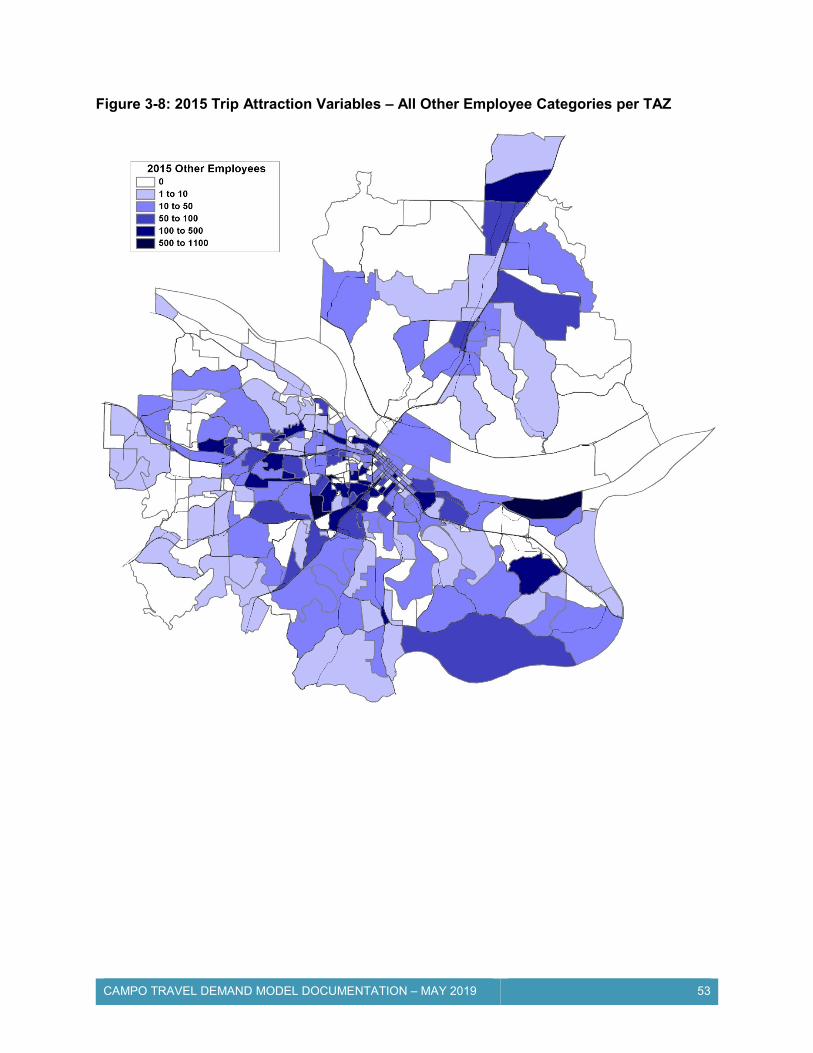
Trip Attractions Trip attraction rates applied in the 2015 Base model were not adjusted from those used in the 2010 Base model. See Chapter 2, Table 2-7 for rates used. Figures 3-5, 3-6, 3-7, and 3-8 illustrated the per-TAZ employees by employment category.
Figure 3-5: 2015 Trip Attraction Variables – Retail Employees per TAZ

CAMPO TRAVEL DEMAND MODEL DOCUMENTATION – MAY 2019 51
Figure 3-6: 2015 Trip Attraction Variables – Office/Service Employees per TAZ

CAMPO TRAVEL DEMAND MODEL DOCUMENTATION – MAY 2019 52
Figure 3-7: 2015 Trip Attraction Variables – Industrial/Warehouse Employees per TAZ
CAMPO TRAVEL DEMAND MODEL DOCUMENTATION – MAY 2019 53
Figure 3-8: 2015 Trip Attraction Variables – All Other Employee Categories per TAZ

CAMPO TRAVEL DEMAND MODEL DOCUMENTATION – MAY 2019 54
External Stations Traffic volumes at the model’s 14 external stations were updated for the 2015 Base model; see Figure 3-9. For some locations, ADT traffic counts were available for 2015. In other locations, historic volume trends or other datasets were used to estimate 2015 volumes.
Table 3-3 contains the External-External (E-E) matrix, or “through” trip matrix, developed for the 2015 daily model. The same procedures used to develop the 2010 EE matrix were applied to develop the 2015 matrix. In addition, the 2015 productions and attractions were balanced using the same procedures as applied in the 2010 Base model.
Figure 3-9: External Station Volumes, 2015 Daily
Rte 179 902 vpd
US-63 22,966 vpd
Rte Y 816 vpd
Rte J 850 vpd
US-54 N 13,000 vpd
Rte. BB 307 vpd
Rte. 94 1,919 vpd
US-50 E 16,258 vpd
Rte W 1,440 vpd
Rte B/E 3,521 vpd
US-54 S 18,431 vpd
Rte C 4,224 vpd
Meadows Ford 1,100 vpd
US-50 W 9,963 vpd

CAMPO TRAVEL DEMAND MODEL DOCUMENTATION – MAY 2019 55
3.4 Trip Distribution The 2015 Base model primarily uses the same trip distribution procedures as the 2010 Base model. As discussed in Chapter 2, the Gravity Model uses a gamma function for travel-time-related impedance. The a, b, and c parameters used as inputs to the gamma function were originally derived from the “Small MPO” values in NCHRP Report 716. However, as noted in Chapter 2, the values were ultimately modified during the 2010 calibration process to better reflect local travel behavior. Further modifications were made during the 2015 calibration process, still keeping in mind reasonable trip length ranges described in both NCHRP 716 and NCHRP 365. The final parameter values are shown in Table 3-4. The average trip lengths that result from these changes to gamma function parameters are displayed in Table 3-5, along with the industry guidelines for reference.
The 2015 Base model continues to make use of the same K-Factor adjustments as were used to increase the attractiveness between certain TAZ pairs in the 2010 Base model. These are described in Chapter 2.
Table 3-4: 2015 Gamma Function Parameters Trip
Purpose a b c
HBW 100 0.265 0.030
HBSCH 100 1.100 0.060
HBSR 100 0.900 0.070
HBO 100 0.900 0.060
NHB 100 1.000 0.100
Table 3-5: 2015 Average Trip Lengths (minutes)
Industry
Guidelines
Trip Purpose
CAMPO Model
NCHRP 716
NCHRP 365
HBW 16.06 20 15-20
HBSCH 12.13 15 11-17
HBSHOP 13.44 18 11-17
HBO 12.91 18 11-17
NHB 10.12 18 11-17
Table 3-3: E-E Matrix – 2015 Daily
401 402 403 404 405 406 407 408 409 410 411 412 413 414 E-E Sum
E-E 2-Way Sum
I-E/E-I Sum
Total External Volume
401 0 1 4 193 3 18 612 8 29 977 41 8 213 5 2,112 4,614 18,346 22,966
402 1 0 0 2 0 0 2 0 0 4 0 0 2 0 11 24 796 816
403 4 0 0 2 0 0 2 0 0 4 0 0 2 0 16 26 830 850
404 193 2 2 0 1 6 249 2 9 420 13 2 281 1 1,182 2,469 10,540 13,000
405 3 0 0 1 0 0 2 0 0 3 0 0 1 0 11 31 267 307
406 18 0 0 6 0 0 6 0 1 12 1 0 6 0 50 96 1,819 1,919
407 612 2 2 249 2 6 0 3 11 430 15 3 290 2 1,626 3,146 13,118 16,258
408 8 0 0 2 0 0 3 0 0 5 0 0 3 0 21 43 1,400 1,440
409 29 0 0 9 0 1 11 0 0 20 1 0 10 0 83 176 3,341 3,521
410 977 4 4 420 3 12 430 5 20 0 28 5 153 4 2,065 3,606 14,831 18,431
411 41 0 0 13 0 1 15 0 1 28 0 0 15 0 117 211 4,004 4,224
412 8 0 0 2 0 0 3 0 0 5 0 0 3 0 22 33 1,060 1,100
413 213 2 2 281 1 6 290 3 10 153 15 3 0 1 980 1,845 8,123 9,963
414 5 0 0 1 0 0 2 0 0 4 0 0 1 0 14 45 862 902
Sum 2,112 11 16 1,182 11 50 1,626 21 83 2,065 117 22 980 14 8,310 16,365 79,337 95,697
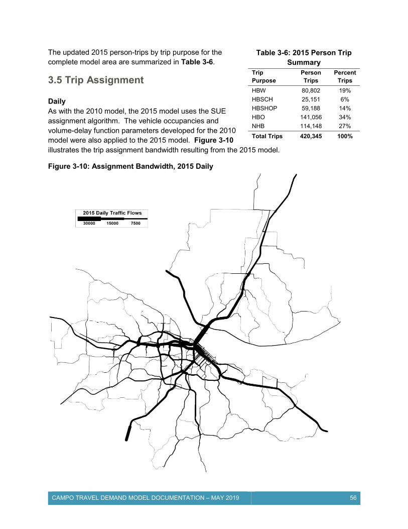
CAMPO TRAVEL DEMAND MODEL DOCUMENTATION – MAY 2019 56
The updated 2015 person-trips by trip purpose for the complete model area are summarized in Table 3-6.
3.5 Trip Assignment Daily As with the 2010 model, the 2015 model uses the SUE assignment algorithm. The vehicle occupancies and volume-delay function parameters developed for the 2010 model were also applied to the 2015 model. Figure 3-10 illustrates the trip assignment bandwidth resulting from the 2015 model.
Figure 3-10: Assignment Bandwidth, 2015 Daily
Table 3-6: 2015 Person Trip Summary
Trip Purpose
Person Trips
Percent Trips
HBW 80,802 19%
HBSCH 25,151 6%
HBSHOP 59,188 14%
HBO 141,056 34%
NHB 114,148 27%
Total Trips 420,345 100%

CAMPO TRAVEL DEMAND MODEL DOCUMENTATION – MAY 2019 57
Peak Hour The 2015 Base model applies the same procedures as the 2010 model to estimate the PM peak hour trips from the daily trips. See Chapter 2 for percentage of daily flows, percentage of departing vs. returning trips, and vehicle occupancies by trip purpose. The resulting 2015 PM vehicle trips by purpose are shown in Table 3-7.
Peak hour link capacities for the 2015 Base model were assumed to be 10 percent of the daily capacities. This same assumption was used in developing the 2010 Base model. An updated PM 2015 E-E matrix was developed and utilized in the assignment of peak hour flows.
The 2010 peak hour model outputs were used to develop turning movement volumes at eleven “critical” intersections determined by CAMPO. These volumes were compared to actual traffic counts, and that comparison led to model adjustments that helped calibrate the 2010 peak hour model. For 2015, no further calibration efforts were made.
No turning movement volumes were developed, nor was intersection analysis was completed with the updated 2015 Base model outputs.
Table 3-7: 2015 PM Vehicle Trips by Purpose
Trip Purpose Trips
HBW 9,731 HBSCH 812
HBSHOP 4,048
HBO 10,111
NHB 6,841
Total 31,543

CAMPO TRAVEL DEMAND MODEL DOCUMENTATION – MAY 2019 58
3.6 Calibration/Validation The 2015 Base model was re-calibrated and validated using the same tests as were initially employed to calibrate the 2010 Base model. These are described in more detail in the following sections.
Percent Assignment Error The assigned 2015 daily traffic volumes were compared with available ADT counts for individual links. Figure 3-11 shows the model links for which ADT counts were available for this comparison.
Figure 3-11: 2015 Link Counts for Model Calibration

CAMPO TRAVEL DEMAND MODEL DOCUMENTATION – MAY 2019 59
The model volumes vs. the actual volumes are plotted on the graph in Figure 3-12. The percent assignment error, which is the difference between the assigned traffic volumes and the counted traffic volumes divided by the counted traffic volumes, is shown in Table 3-8. The percent error of the traffic assignment is -1.8% overall, and the percentages for each functional class are within acceptable ranges.
Figure 3-12: Predicted vs. Actual Volumes
Coefficient of Determination (R2) The R2 statistic is also displayed on Figure 3-12. The achieved value of 0.918 is above the desirable threshold of 0.88, indicating a good fit between the model output and the available counts.
Root Mean Square Error (RMSE) RMSE is another way of comparing the assigned model traffic to the counted traffic volumes, by measuring the deviation between the two. The percent RMSE by volume range for 2015 is shown in Table 3-9. As noted in Chapter 2, there are no national standards for model verifications of RMSE. The 2010 Base model utilized guidelines provided by the state of Tennessee as a resource for validating. The updated 2015 Base model results also meet those recommended guidelines.
Table 3-8: Percent Assignment Error – 2015 Daily
Percent Error
Functional Class Computed
Suggested Range*
Freeway 1.7% +7%
Primary Arterial -5.3% +10%
Collector -14.2% +25%
Local 12.2% +25%
Overall -1.8% +5%
*Source: Calibration and Adjustment of System Planning Models, Federal Highway Administration, December 1990.
Table 3-9: Percent Root Mean Square Error (RMSE) – 2015 Daily Volume Ranges RMSE Guidelines*
20,000 to 39,999 14.4% 25.4%
10,000 to 19,999 16.3% 28.3%
5,000 to 9,999 27.5% 43.1%
0 to 4,999 48.0% 115.8%
Overall 29.5% 30.0%
*Source: Minimum Travel Demand Model Calibration and Validation Guidelines for State of Tennessee
R² = 0.9183
0
10000
20000
30000
40000
50000
0 10000 20000 30000 40000 50000

CAMPO TRAVEL DEMAND MODEL DOCUMENTATION – MAY 2019 60
Screenline Analysis The screenline analysis again compares the results of the model trip assignment to the daily traffic counts, but for specific locations, across logical travel routes. The same five screenlines utilized in the 2010 Base model calibration process were also used for the updated 2015 Base model; see Chapter 2 for a map of locations. FHWA provides guidelines for the percent allowable deviation of the total model volumes along a screenline to the total daily counts along the same screenline. The allowable deviation is based on the total traffic volume (lower volumes allow for a greater deviation). At each of the screenlines, the results for the 2015 Base model fall well within the allowable ranges, as shown in Table 3-10.
Table 3-10: Screenline Analysis – 2015 Daily
Screenline Model
Volume Traffic Count % Diff
FHWA Allowable %
North 17,649 17,270 2% ± 45%
River 61,503 53,991 14% ± 30%
Southeast 64,147 63,868 0% ± 30%
Southwest 106,548 114,460 -7% ± 22%
Downtown 231,056 210,275 10% ± 18%
Total 480,903 459,864 5%

CAMPO TRAVEL DEMAND MODEL DOCUMENTATION – MAY 2019 61
Chapter 4: 2045 Model Scenarios
4.1 Scenario Planning In order to determine what the future of the CAMPO region may look like, CAMPO staff, with the assistance of the consultant team, undertook a scenario planning exercise. Scenario planning is a process that helps a community to establish a vision and implement a strategic plan that considers and prepares for possible challenges and opportunities well into the future.
Items considered in the development of a scenario include:
Population growth Land-Use changes Transportation investments Demographic shifts (e.g., aging population) Economic growth and shifts Housing preferences Fuel prices Technological developments (e.g., alt. fuels)
With input from the public and stakeholders, CAMPO developed and analyzed four scenarios using the CommunityVIZ scenario planning software.
Trend Scenario – This scenario extends current growth patterns into the future. It included a mixture of growth in undeveloped fringe areas, as well as infill-type growth in currently developed areas.
Central City Development – This scenario generally concentrated more growth in the center of Jefferson City and Holts Summit than the Trend scenario.
Unincorporated Development – This scenario generally concentrated more growth in unincorporated areas than the Trend scenario.
Aggressive Growth – This scenario assumed much more aggressive growth rates, more than double those of the other scenarios. This scenario was somewhat of a “stress-test” on the region’s systems over the coming decades.
For purposes of comparing the four scenarios, Table 4-1 shows some of the residential metrics that came out of the scenario planning exercise. This type of information, as well as updated employment information, was then fed into the 2045 travel demand model for each scenario.
Table 4-1: New Residential Development by Scenario
Trend Central City
Development Unincorporated
Development Aggressive
Growth
Total Residential 6,800 6,800 6,800 14,467
Multi-Family Residential 367 404 381 1,926
Residential Near Employment Centers 3,001 3,302 2,848 5,826
Residential as part of Mixed Use Development 685 911 463 1,146
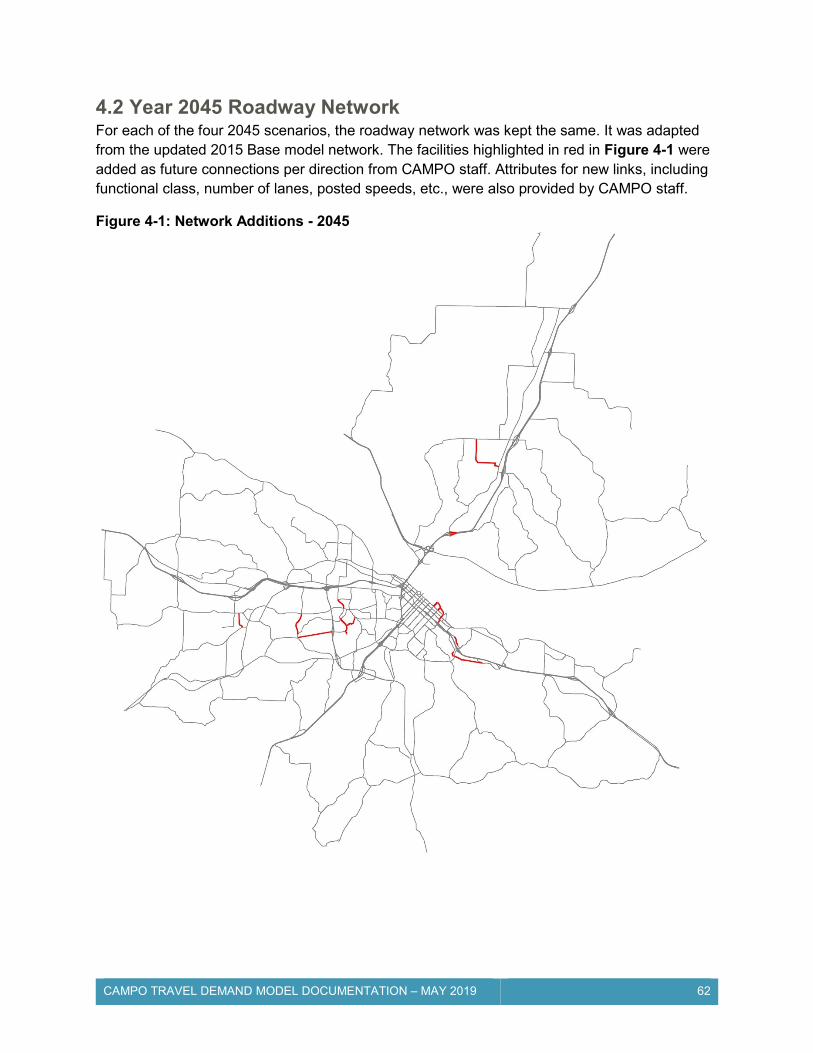
CAMPO TRAVEL DEMAND MODEL DOCUMENTATION – MAY 2019 62
4.2 Year 2045 Roadway Network For each of the four 2045 scenarios, the roadway network was kept the same. It was adapted from the updated 2015 Base model network. The facilities highlighted in red in Figure 4-1 were added as future connections per direction from CAMPO staff. Attributes for new links, including functional class, number of lanes, posted speeds, etc., were also provided by CAMPO staff.
Figure 4-1: Network Additions - 2045
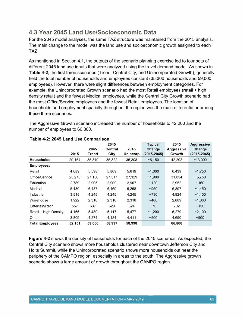
CAMPO TRAVEL DEMAND MODEL DOCUMENTATION – MAY 2019 63
4.3 Year 2045 Land Use/Socioeconomic Data For the 2045 model analyses, the same TAZ structure was maintained from the 2015 analysis. The main change to the model was the land use and socioeconomic growth assigned to each TAZ.
As mentioned in Section 4.1, the outputs of the scenario planning exercise led to four sets of different 2045 land use inputs that were analyzed using the travel demand model. As shown in Table 4-2, the first three scenarios (Trend, Central City, and Unincorporated Growth), generally held the total number of households and employees constant (35,300 households and 59,000 employees). However, there were slight differences between employment categories. For example, the Unincorporated Growth scenario had the most Retail employees (retail + high density retail) and the fewest Medical employees, while the Central City Growth scenario had the most Office/Service employees and the fewest Retail employees. The location of households and employment spatially throughout the region was the main differentiator among these three scenarios.
The Aggressive Growth scenario increased the number of households to 42,200 and the number of employees to 66,800.
Table 4-2: 2045 Land Use Comparison
2015 2045 Trend
2045 Central
City 2045
Unincorp
Typical Change
(2015-2045)
2045 Aggressive
Growth
Aggressive Change
(2015-2045)
Households 29,164 35,319 35,322 35,308 ~6,150 42,202 ~13,000
Employees:
Retail 4,689 5,598 5,809 5,619 ~1,000 6,439 ~1,750
Office/Service 25,275 27,156 27,317 27,129 ~1,900 31,034 ~5,750
Education 2,789 2,905 2,909 2,907 ~120 2,952 ~160
Medical 5,430 6,437 6,469 6,268 ~950 6,897 ~1,450
Industrial 3,515 4,245 4,245 4,245 ~730 4,924 ~1,400
Warehouse 1,922 2,318 2,318 2,318 ~400 2,889 ~1,000
Entertain/Recr 557 637 629 624 ~70 702 ~150
Retail – High Density 4,165 5,430 5,117 5,477 ~1,200 6,279 ~2,100
Other 3,809 4,274 4,184 4,411 ~500 4,690 ~900
Total Employees 52,151 59,000 58,997 58,998 66,806
Figure 4-2 shows the density of households for each of the 2045 scenarios. As expected, the Central City scenario shows more households clustered near downtown Jefferson City and Holts Summit, while the Unincorporated scenario shows more households out near the periphery of the CAMPO region, especially in areas to the south. The Aggressive growth scenario shows a large amount of growth throughout the CAMPO region.

CAMPO TRAVEL DEMAND MODEL DOCUMENTATION – MAY 2019 64
Figure 4-2: 2045 Household Density
For each of the 2045 scenarios, the average household size, and the number of households within each size range, were held to the same ratios as the 2015 Base model.
Trend Scenario Central City Growth
Unincorporated Growth Aggressive Growth

CAMPO TRAVEL DEMAND MODEL DOCUMENTATION – MAY 2019 65
Figure 4-3 shows the employment density for each of the 2045 scenarios. Development patterns are similar to those shown in the household density maps.
Figure 4-3: 2045 Employment Density
Trend Scenario Central City Growth
Unincorporated Growth Aggressive Growth

CAMPO TRAVEL DEMAND MODEL DOCUMENTATION – MAY 2019 66
4.4 2045 Trip Generation Trip generation for 2045 uses the same procedures employed in the 2015 Base model. The same five trip purposes are used, and the trip production/attraction rates are carried forward. Table 4-3 summarizes the estimated productions and attractions by purpose for each of the 2045 scenarios. As would be expected, the Trend, Central City, and Unincorporated scenarios have similar numbers of productions and attractions, while the Aggressive Growth scenario has significantly more.
External volumes were projected to 2045 using historical growth rates, extrapolated forward in a reasonable manner on a location-specific basis. Table 4-4 includes the 2045 E-E matrix. This same matrix was used for all of the 2045 scenarios.
Table 4-4: 2045 E-E Matrix
401 402 403 404 405 406 407 408 409 410 411 412 413 414 E-E Sum
E-E 2-Way Sum
I-E/E-I Sum
Total External Volume
401 0 2 6 261 5 24 843 10 37 1249 54 11 293 7 2,802 7,298 26,766 34,066
402 2 0 0 2 0 0 2 0 0 5 0 0 2 0 14 33 1,076 1,116
403 6 0 0 3 0 0 3 0 0 4 1 0 3 0 20 35 1,110 1,150
404 261 2 3 0 2 7 307 3 11 471 15 3 344 2 1,429 3,032 12,660 15,700
405 5 0 0 2 0 0 3 0 0 4 1 0 2 0 18 61 547 607
406 24 0 0 7 0 0 8 0 1 13 1 0 8 0 62 111 2,099 2,219
407 843 2 3 307 3 8 0 3 12 493 17 3 362 2 2,060 4,062 16,398 20,458
408 10 0 0 3 0 0 3 0 0 6 0 0 3 0 26 52 1,680 1,740
409 37 0 0 11 0 1 12 0 0 21 2 0 12 0 98 191 3,621 3,821
410 1249 5 4 471 4 13 493 6 21 0 30 6 173 4 2,480 3,671 15,051 18,731
411 54 0 1 15 1 1 17 0 2 30 0 0 17 0 138 226 4,304 4,524
412 11 0 0 3 0 0 3 0 0 6 0 0 3 0 28 42 1,360 1,400
413 293 2 3 344 2 8 362 3 12 173 17 3 0 2 1,224 2,325 10,043 12,363
414 7 0 0 2 0 0 2 0 0 4 0 0 2 0 18 60 1,142 1,202
Sum 2,802 14 20 1,429 18 62 2,060 26 98 2,480 138 28 1,224 18 10,417 21,199 97,857 119,097
Table 4-3: 2045 Productions + Attractions by Purpose
Trip Purpose 2015 2045 Trend
2045 Central City
2045 Unincorporated
Typical New Trips
2045 Aggressive Growth
Aggressive New Trips
HBW 161,604 197,586 197,129 197,945 ~36,000 222,710 ~61,100
HBSCH 50,302 61,465 60,889 61,636 ~11,000 73,315 ~23,000
HBSHOP 118,376 144,429 143,802 144,493 ~25,900 165,860 ~47,500
HBO 282,112 343,719 342,131 344,377 ~61,300 405,416 ~123,300
NHB 228,296 277,610 276,040 277,699 ~48,800 329,622 ~101,300
Total 840,690 1,024,809 1,019,991 1,026,149 1,196,923

CAMPO TRAVEL DEMAND MODEL DOCUMENTATION – MAY 2019 67
4.5 2045 Trip Distribution The 2045 models used the same trip distribution procedures used for the 2015 (and 2010) models; the gravity formulation, friction factors, and K-factors used for those models were retained for 2045 conditions. The total 2045 person-trips by purpose are shown in Table 4-5.
4.6 2045 Trip Assignment Daily Assignment Daily trips were assigned in the 2045 model scenarios using the SUE assignment algorithm. The vehicle occupancies and volume-delay function parameters developed for the 2015 Base model were also applied to the 2045 model. The capacities for each roadway link were compared to the assigned volumes to determine a V/C ratio and corresponding level of service. Road facilities with a V/C ratio or greater than 0.9 (LOS E or F) were considered to be congested. Figure 4-4 illustrates the congested roads for each of the four 2045 scenarios.
As shown, the variations between the Trend, Central City Growth, and Unincorporated scenarios resulted in little to no change regarding roadway congestion. The aggressive growth scenario, due to the large increase in total trips, does show some additional congested roadways.
Table 4-5: 2045 Person Trip Summary Trip Purpose Trend
Central City
Unincorporated Growth
Aggressive Growth
Percent Trips
HBW 98,793 98,565 98,973 111,355 19%
HBSCH 30,733 30,445 30,818 36,658 6%
HBSHOP 72,215 71,901 72,246 82,930 14%
HBO 171,860 171,065 172,188 202,708 34%
NHB 138,805 138,020 138,849 164,811 27%
Total Trips 512,405 509,996 513,075 598,462 100%

CAMPO TRAVEL DEMAND MODEL DOCUMENTATION – MAY 2019 68
Figure 4-4: 2045 Congested Roadways
Trend Scenario Central City Growth
Unincorporated Growth Aggressive Growth

CAMPO TRAVEL DEMAND MODEL DOCUMENTATION – MAY 2019 69
4.7 Selected Scenario
With the aid of the public/stakeholder involvement process, it was decided that the Trend scenario was the most likely growth scenario for the CAMPO region. Therefore, future planning endeavors are using the outputs of that scenario.
Figure 4-5 illustrates the model-projected traffic flows and volume-to-capacity ratios expected on a daily basis, by 2045, with the Trend scenario.
Figure 4-5: 2045 Trend Scenario Daily Assignment Bandwidth with V/C

CAMPO TRAVEL DEMAND MODEL DOCUMENTATION – MAY 2019 70
PM peak-hour turning-movement volumes were extracted from the 2045 Trend Scenario model for each of the study intersections identified by CAMPO (as described in Chapter 2). The raw volumes were post-processed to account for deviations between the Base 2010 model outputs and counts available from that time period. The resulting volumes are shown in Figure 4-6.
Figure 4-6: 2045 Trend Scenario PM Peak Hour Turning Movement Volumes
The 2045 turning movement volumes were then analyzed using the Synchro software. The results of this operational analysis are shown in Table 4-6. As the table shows, the intersection of the US-54 southbound ramps and Simon Boulevard is forecasted to operate at LOS F by 2045. The long delays at this intersection would likely be mitigated with installation of a traffic signal. Each of the other study intersections is expected to operate acceptably, although individual movements are expected to fail at three of the intersections, as noted in the table.

CAMPO TRAVEL DEMAND MODEL DOCUMENTATION – MAY 2019 71
Table 4-6: 2045 PM Peak our Intersection Analysis
Sig/Unsig* Delay LOS
1. US-54 SB Ramps & Simon Blvd U 505.3 (SB) F
2. Missouri Blvd EB Ramps & Rte. 179 S 14.9 B
3. US-50 EB/Horner Rd & Truman Blvd S 27.8 C
4. Stadium Blvd & Jefferson St Rdbt 12.3 B
5. Missouri Blvd & Dix Rd S 51.1 D#
6. Missouri Blvd & Beck St S 33.2 C#
7. US-54 NB Ramps & Ellis Blvd S 47.7 D#
8. US-50/63 EB Ramps & Eastland Dr S 18.1 B
9. Rte. B/W/M** U 34.2 (WB) D
10. US-50/63 WB Ramps & Militia Dr U 0.0 (WB) A
11. US-50 EB/Horner Rd & Big Horn Dr U 17.0 (WB) C
* For unsignalized intersections the delay/LOS reported is for the worst movement at the intersection ** Intersection 9 was analyzed as a two-way stop (east-west stop) because Synchro does not allow analysis of the actual configuration (3-way stop at a 4-way intersection).
# One or more movements operate at LOS E or F.

CAMPO TRAVEL DEMAND MODEL DOCUMENTATION – MAY 2019 72
Chapter 5: Capital Improvement Projects The 2045 Trend Scenario model results were used to assist in the development of a representative list of future projects for inclusion in the CAMPO 2045 Metropolitan Transportation Plan (MTP). However, the model was not the only source underlying this list. The list was developed for both near- and long-term projects, and travel-demand models are not designed to develop near-term recommendations. The 2015 Base-year model was developed with the sole purpose of calibrating the model to allow development of future projections. There are better means to establish near-term needs. The two methods used to examine near-term needs for the MTP included:
Google congestion maps: Google’s traffic maps have a historical feature that allows the viewing of “typical” traffic conditions for any day of the week, and any time of day. Figure 5-1 displays a compilation of Google traffic data, showing the “worst case” in terms of speeds that each roadway experiences throughout the day. Several areas of congestion are indicated by the slow speeds. Figure 5-1: Google Maps “Typical” Traffic Conditions
“Fast” “Slow”

CAMPO TRAVEL DEMAND MODEL DOCUMENTATION – MAY 2019 73
Stakeholder input: Perhaps the most valuable indicator of near-term needs is input from
the agencies charged with oversight and maintenance of the roadway system, and from members of the community who utilize the roads throughout the CAMPO region on a daily basis. Input on project needs was gathered at two public meetings, as well as an online survey. Figure 5-2 visually displays each of the comments and ideas brought forth by these stakeholders. Figure 5-2: Stakeholder Input

CAMPO TRAVEL DEMAND MODEL DOCUMENTATION – MAY 2019 74
The 2045 model did have the ability to verify a number of the capacity-related short-term improvements, because typically an existing over-capacity situation will also show up in a model as a long-term issue. More importantly, the model is generally a better indicator of long-term needs, including some that stakeholders may not yet have envisioned because the needs haven’t yet materialized. Figure 5-3 displays the areas with poor LOS as projected by the 2045 Trend Scenario models. In many cases, the model results align with and support the stakeholder-provided issues – and also identify other potential issues. Both the Daily and PM peak models were referenced in developing a recommended list of capital projects, through examination of segments projected to operate at LOS E and F to determine whether a future improvement project would make sense at a given location. Table 5-1 contains the list of recommended capacity projects, categorized by near-term and long-term. The list also contains the location, project type, length (if applicable), description, and a rough order-of-magnitude cost range for each project. This list is not CAMPO’s final list of regional transportation improvement recommendations; outside this document, it has been further developed and enhanced by CAMPO, including the addition of non-automobile-capacity projects, for incorporation into the Metropolitan Transportation Plan (MTP).
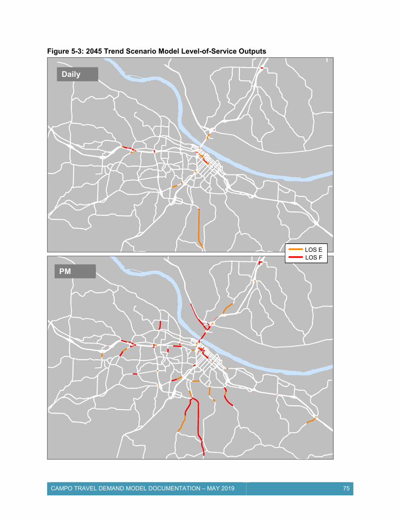
CAMPO TRAVEL DEMAND MODEL DOCUMENTATION – MAY 2019 75
Figure 5-3: 2045 Trend Scenario Model Level-of-Service Outputs
Daily
PM
LOS E LOS F

CAMPO TRAVEL DEMAND MODEL DOCUMENTATION – MAY 2019 76
Table 5-1: CAMPO – Capacity Projects List From Traffic Modeling Team
Near-Term (5-10 years)
Location Facility Type
Length (mi)
County/City Size Project
US 50 / Truman Bl / Country Club Dr
Interchange - Jefferson City Large -
Very Large
Reconfigure interchange to address close outer road spacing; widen westbound off-ramp to improve capacity; incorporate pedestrian facilities into the interchange
US 50 / Dix Rd Interchange - Jefferson City Large
Reconfigure interchange and Dix Rd approaches to address capacity issues including lack of left-turn lanes; consider dumbbell roundabout interchange; widen Dix Rd to provide center turn lane from US 50 to Missouri Bl
US 50/63 / Clark Ave Interchange - Jefferson City Moderate -
Large
Reconfigure interchange to address ramp terminal capacity (likely roundabouts); include modifications to Clark/Miller and Clark/Dunklin intersections to improve corridor operations
US-54 NB Ramps / Christy Dr / Lorenzo Green / Jefferson St
Interchange - Jefferson City Moderate -
Large
Install roundabouts at both hook ramp intersections to improve operations and address offsets/angles
US 54 / Ellis Bl / Southwest Bl
Interchange - Jefferson City Large -
Very Large
Reconfigure interchange to address capacity and close spacing of outer roads. Create a pedestrian connection along Southwest Bl / Ellis Bl from Ford St to Southridge Dr
Missouri Blvd, Eastern Lowe's entrance to S 10 Mile Dr
Segment 0.4 Jefferson City Moderate-
Large
Widen to add a center turn lane to improve capacity and safety. Address access management along the corridor, including turn restrictions and additional traffic control.
Route B, Tanner Bridge Rd to Friendship Rd
Segment 2.78 Wardsville Large -
Very Large
Install roundabouts at two locations to improve capacity: Rte B / Falcon / Ashbury, Rte B / Rte M; widen to four lanes in each direction on Rte B for several hundred feet south of Tanner Bridge Rd and reconfigure intersection; Widen Rte B to provide TWLTL between Falcon /Ashbury and Rte M; consider consolidating Ashbury / Friendship west of Rte B
Madison Street, Dunklin St to US-54 Ramps
Segment 0.5 Jefferson City Moderate
Add a center turn lane via a combination of widening and parking removal; address unusual stop control configuration at Madison Atchison
W. Truman Blvd / Scott Station Rd
Segment 0.3 Jefferson City Very Small Signalize or otherwise enhance capacity
Ellis Bl / Green Berry Rd Intersection - Jefferson City Small -
Moderate Install roundabout to improve intersection capacity
Bald Hill Rd / Seven Hills Rd
Intersection - Jefferson City Small -
Moderate Install roundabout to improve intersection capacity

CAMPO TRAVEL DEMAND MODEL DOCUMENTATION – MAY 2019 77
Long-Term (10+ years)
Location Facility Type
Length (mi)
County/City Size Project
US 50 / 63 / 54 (Tri-Level)
Interchange - Jefferson City Large -
Very Large Reconfigure interchange to provide non-conflicting system-to-system movements
US 50/63, US 54 to Lafayette St
Segment 1.2 Jefferson City Very Large Implement major capacity improvements, which could include mainline widening, grade separations, and/or outer roads
US 54 / 63 / 94 (Bluff Rd)
Interchange - Jefferson City Very Large
Construct direct connector for northbound-to-westbound movement to improve capacity; widen US 54/63 to provide 3 continuous through lanes in each direction (in addition to auxiliary/accel/decel lanes)
US 54 / Route OO / Simon Bl
Interchange - Holts Summit Large
Reconfigure interchange to address close outer road spacing and capacity issues (may involve roundabouts); incorporate pedestrian facilities crossing US 54
US 54 / Center St Interchange - Holts Summit Moderate -
Large
Improve interchange capacity and east-side outer road spacing with roundabouts at terminals
Missouri Blvd, Country Club Dr to Howerton Ct
Segment 0.4 Jefferson City Large Widen to 5 lanes
Country Club Dr, Truman Bl to Rainbow Dr
Segment 0.5 Jefferson City Moderate Widen to provide left-turn lanes at existing and future access points
Country Club Dr, Fairway Dr to Country Ridge Dr
Segment 0.33 Jefferson City Small -
Moderate
Restripe (and potential minor widening) to provide center turn lane to improve capacity and safety
Rock Hill Rd, Industrial Dr to Sue Dr
Segment 0.6 Jefferson City Small -
Moderate Add left-turn lanes at Sue Dr, Cherry Creek Ct, and Fire Station north driveway
Rock Ridge Rd / Wildwood Dr extension
Intersection - Cole County Small Add left-turn lane on Rock Ridge to improve capacity
Project Sizes
Cost Range
Very Small < $500k
Small $500k - $1M
Moderate $1M - $5M
Large $5M - $10M
Very Large > $10M

CAMPO TRAVEL DEMAND MODEL DOCUMENTATION – MAY 2019 78
Chapter 6: Model Procedures
6.1: General Model Flowchart Figure 6-1 summarizes the CAMPO model process. Filenames not mentioned in this figure are not active in the model and may serve as placeholders for future implementation.
Trip Generation
Network Skimming
Initialization (Network)
Network File Network_xx.net
Production Trip Rates TG RatesP xx bin
IE Table IE xx bin
Balanced PA Table PA xx.bin
Attraction Trip Rates TG RatesA xx.bin
Unbalanced P/A Tables UnbalancedP_xx.bin UnbalancedA xx.bin
Shortest Path Matrix skim_xx.mtx
Gravity Model (Trip Distribution)
TAZ Layer TAZ xx dbd
K-Factors KFactors_xx.mtx Peak-Hour (Diurnal)
Distribution Hourly.bin
PA Matrix pa_xx.mtx
OD Matrix od_xx.mtx
Cross-classification (HH and Autos)
Through Trips ee_xx.mtx
Assignment assign_AM_xx.bin assign_PM_xx.bin assign_D_xx.bin
Turn Movements turns_AM_xx.bin turns_PM_xx.bin turns_D_xx.bin
PA to OD conversion
Person-trip to veh-trip conversion
Capacity Table Capacity xx.bin
Highway Layer Modelnetwork xx.dbd
Global Turn Penalties TURN PENALTY TYPE_xx.dbf
Specific Turn Penalties TURN PENALTY RESTR xx.dbf
Trip Assignment
Figure 6-1: CAMPO Model Process
TLDs by Purpose TLD –
[PURP]Time_xx.mtx

CAMPO TRAVEL DEMAND MODEL DOCUMENTATION – MAY 2019 79
6.2: File/Folder Structure Figure 6-2 summarizes the CAMPO model files and folder structure. The fundamental folder and file structure must remain as described in the figure. Any changes to directories or file names will result in model run errors. This structure also facilitates file maintenance amongst users.
TDM
Local Disk (C:)
CAMPO
Archive
Scenarios
2015
2045A
2045B
Temp
Script
Output
Output
The Archive folder stores previous model run files in subfolders. Subfolders populate when the interface “Archive” button is utilized by the model user.
The Scenarios folder stores input and output model files by scenario name and time of day. It also stores the “HOURLY” table and “ScenarioList.txt” files. Initially, base scenario folders (i.e. 2015, 2045 A-D) and files must be populated by the user. Other scenario folders and files can be populated by the user or by the interface via the “Save Scenario As” button. Folder names determine the last portion of all the model file names (i.e. file names in the 2015 folder end with “_2015”).
The input set of model files is located in these scenario folders. The “Output” subfolders are populated by the script when the model is run. The “Output” subfolders contain the output set of model files.
The folder names correspond to the Scenario Planning scenarios as follows:
2045A: Central City Growth 2045B: Unincorporated Growth 2045C: Trend Scenario 2045D: Aggressive Growth
The Temp folder contains the files that are used directly by the model while the model runs. It is not intended for the user to modify the files in this folder.
The Script folder contains the main script files and related files. These files should be handled carefully.
Output
Figure 6-2: CAMPO File/Folder Structure
2045C
2045D
Output
Output

CAMPO TRAVEL DEMAND MODEL DOCUMENTATION – MAY 2019 80
6.3: Basic Setup Please complete these steps before attempting your first model run.
1. Create the folders listed below: Folder Directory Can User Modify Contents? Folder Description C:\TDM\Script No All custom and standard script files.
Please consult with the HDR team if changes need to be made.
C:\TDM\CAMPO
-- The main directory for this TransCAD model.
C:\TDM\CAMPO\Archive
Yes In the TransCAD dialog box, there will be an option to auto-Archive model run files and an Archive button. This is where the files will be stored. Each set of files will have a folder name with its archival date.
C:\TDM\CAMPO\Scenarios
Scenario folder contents – Yes File names – No (these are dependent on the scenario folder name)
All scenario folders and files will reside here. You can manage your own scenario folders/files or use the scenario manager buttons in the dialog box.
C:\TDM\CAMPO\Temp
No These are temporary files that TransCAD uses during the runs.
C:\TDM\CAMPO\Scenarios\2015 Scenario folder contents – Yes File names – No (these are dependent on the scenario folder name)
All input Existing Conditions files. An “Output” subfolder will be created by the script for the output files.
C:\TDM\CAMPO\Scenarios\2045A Scenario folder contents – Yes File names – No (these are dependent on the scenario folder name)
All input 2045A files. A subfolder will be created by the script for the output files.
C:\TDM\CAMPO\Scenarios\2045B Scenario folder contents – Yes File names – No
All input 2045B files. A subfolder will be created by the script for the output files.
C:\TDM\CAMPO\Scenarios\2045C Scenario folder contents – Yes File names – No
All input 2045C files. A subfolder will be created by the script for the output files.
C:\TDM\CAMPO\Scenarios\2045D Scenario folder contents – Yes File names – No
All input 2045D files. A subfolder will be created by the script for the output files.
2. Note the path and folder name for your TransCAD folder.
Folder Directory Can User Modify Contents? Folder Description C:\Program Files\-enter your TransCAD folder name here-
Folder contents – Yes File names – No
This folder is where the TransCAD software is installed; the directory name varies depending on what the user named the folder upon installation. It is where TransCAD looks for essential behind-the-scenes files.

CAMPO TRAVEL DEMAND MODEL DOCUMENTATION – MAY 2019 81
3. Place all files in zip file “Script” under: C:\TDM\Script. Delete or archive old files in this folder if any exist.
4. Place “ScenarioList.txt”, “HOURLY.BIN”, and “HOURLY.DCB” in C:\TDM\CAMPO\Scenarios\.
5. Place “campo.ini” in your TransCAD folder: C:\Program Files\-enter your TransCAD folder name here-
6. Place all files in the zip file “2015” in C:\TDM\CAMPO\Scenarios\2015\. Delete or archive any old files in this folder if any exist.
7. Place all files in the zip file “2045A” in C:\TDM\CAMPO\Scenarios\2045A\. Delete or archive any old files in this folder if any exist.
8. Repeat step 7 for scenarios 2045B, 2045C and 2045D.
9. If your TransCAD folder is not named “TRANSCAD FULL”, you have two choices: 1. Rename it to “TRANSCAD FULL”. 2. Open your TransCAD folder and find “campo.ini” (you placed it there in step 5).
Open “campo.ini”. It should open up with Notepad or any other text editor. Change the directory listed under “[UI File]” to “C:\Program Files\-enter your TransCAD folder name here-\campo.dbd”. If you do not yet have a campo.dbd file in your TransCAD folder, do not be alarmed. We will create it in the next section.
Compilation From this point forward you will need a TransCAD Standard Key (USB device). If you have not run a TransCAD model via script files, this section will be helpful. Please follow these steps in order. You should only need to do this setup once. These steps only need to be repeated if script files are changed.
1. Open TransCAD. Go to Tools > GIS Developer’s Kit. The kit will appear as a dialog box or docked on the taskbar.
2. Click the “Compile to UI” button, which is the third button from the left. 3. Browse to “C:\TDM\Script\” and select “campo_compile_list.lst”. Click the “Open”
button. 4. In the next dialog box, browse to “C:\Program Files\-enter your TransCAD folder
name here-”. Type in “campo.dbd” and click “Save”. Click “Yes”/“OK” at the prompt.
Dialog Box Docked on the taskbar

CAMPO TRAVEL DEMAND MODEL DOCUMENTATION – MAY 2019 82
If you encounter any errors or questionable pop-up messages during this process, please make sure you have followed all the steps in this section correctly. If the errors persist, please notify the HDR team and we will assist you. Add-in This subsection outlines steps to setup access to the Dialog Box (also known as “Graphical User Interface”) from which you can do a model run.
1. Go to Tools > Setup Add-ins… 2. Click the “Add” button. 3. Settings:
1. Type: Dialog Box 2. Description: CAMPO 3. Name: CAMPO Model 4. UI Database:
C:\Program Files\C:\Program Files\-enter your TransCAD folder name here-\campo.dbd
5. In Folder: None 4. Click “OK”.
6.4: Running the Model To complete a model run using our custom Dialog Box (shown at right), please follow these instructions.
1. In TransCAD, go to Tools > Add-ins > CAMPO (After a few uses, TransCAD will create a shortcut directly under the Tools drop down menu called “CAMPO”). The Dialog Box should appear.
2. Click the “Open Scenario” button. Select the desired scenario (i.e. 2015, 2045A, etc.). Click “OK”. A status bar should appear.
3. The text at the top of the CAMPO Travel Demand Model dialog box should read: “Scenario: 2015” or whichever scenario is chosen.
4. This step is only a check that the directories and file names have loaded properly. Click the “Setup” button. The “Project Scenarios” box should appear. An image of the “Project Scenarios” box is shown below.
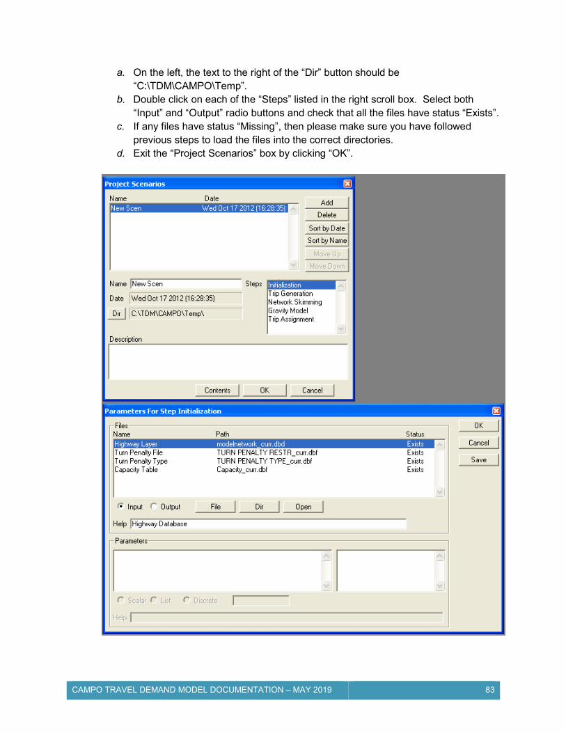
CAMPO TRAVEL DEMAND MODEL DOCUMENTATION – MAY 2019 83
a. On the left, the text to the right of the “Dir” button should be “C:\TDM\CAMPO\Temp”.
b. Double click on each of the “Steps” listed in the right scroll box. Select both “Input” and “Output” radio buttons and check that all the files have status “Exists”.
c. If any files have status “Missing”, then please make sure you have followed previous steps to load the files into the correct directories.
d. Exit the “Project Scenarios” box by clicking “OK”.

CAMPO TRAVEL DEMAND MODEL DOCUMENTATION – MAY 2019 84
5. Interface and Checkboxes: a. Stop after each stage. A “stage” is a model step (i.e. “Initialization”, “Trip
Generation”, etc.). If this box is checked, only the model step selected by the user is run. If this box is unchecked, the model step selected by the user as well as subsequent model steps are run continuously.
b. Time of day procedure. By selecting this checkbox, the model steps “Gravity Model” and “Trip Assignment” will include appropriate procedures to output peak hour results.
6. Run the model by clicking “Initialization” then “Trip Generation” then “Network Skimming” etc.
7. Additional buttons not yet mentioned: a. Archive. This button will archive the latest model output files for the scenario listed
shown at the top of the Dialog Box. Those files are copied into a subfolder in “C:\TDM\CAMPO\Archive”. The subfolder is named with the archival time and date.
b. Save Scenario As. This button will allow you to create a new scenario. When you use “Save Scenario As”, a window will prompt you to manually create a new scenario folder. The new scenario folder needs to be located under the directory “C:\TDM\CAMPO\Scenarios\”. Then the script will auto rename and save your files in the new folder based on the new folder’s name. The button is also helpful to start a whole new set of files, which you can edit for your new scenario.

CAMPO TRAVEL DEMAND MODEL DOCUMENTATION – MAY 2019 85
6.5: Network Changes: Modifying/Adding Links To make changes to the network, open and modify the file “modelnetwork_(scenario name).dbd”. If making any changes to existing base conditions, make sure to make the same changes to the future years’ base scenarios networks as well. When editing link attributes, please make sure all of the attributes in the table below are updated. When adding a link, use the TransCAD Map Editing tool and populate all fields below. The Fields in the network file not mentioned below were referenced by HDR during model development.
Be sure to check loading onto new links and add new centroid connectors if applicable. Be aware that the properties of existing centroid connectors are tied to the calibrated existing conditions model. Also note that centroid connector lengths affect the amount of traffic distributed amongst centroid connectors. Generally, for a TAZ, more traffic will be attracted to the TAZ’s shorter centroid connector compared to its longer centroid connector. However, there are other variables that affect the resulting volumes on these connectors.
Attribute (Field Name) Description Notes Dir* One-way (1, -1) or Two-way (0) To define a one way link, change your link layer
attributes to show “Topology”. Dir = 1 agrees with the topology arrows. Dir = -1 opposes the topology. The link layer attributes “Direction of flow” arrow is based on the “Dir” value.
Street Name Street Name -- FunClass 1 = Freeways
3 = Arterials 5 = Collectors 6 = Local 7 = Ramps 8 = System Ramps 9 = Centroid Connectors
Roadway Functional Classification Numbers. Numbers 2 and 4 are typically used for expressways and minor arterials respectively. They are not currently used by the model, but the numbers are reserved for future implementation. When the minor arterials classification is used, functional class 3 represents major arterials.
Area Type
1 = CBD 2 = Non-CBD
To determine the Area Type, refer to the Area Type figure in Chapter 2.
Median Type
1 = Undivided 2 = Undivided with turn lanes at intersections 3 = TWLTL (two-way left-turn lane) 4 = Raised Median – No turn lanes 5 = Raised Median – With turn lanes
The type of median located on the link.
AB_Lane** BA_Lane**
Number of Lanes The number of lanes in the AB or BA direction.
AB_Speed** BA_Speed**
Posted Speed and/or Free-Flow Travel Speed
The posted and/or free-flow travel speed in the AB or BA direction.
ADT (Only modify for new links)
Daily Traffic Counts Used for calibration. Please do not modify for existing links.
* The topology is determined by the way the link was originally drawn when the link was created. **AB_ indicates traffic flow that is consistent with the link’s topology. BA_ indicates traffic flow opposite the link’s topology.

CAMPO TRAVEL DEMAND MODEL DOCUMENTATION – MAY 2019 86
6.6: TAZ Changes: Modifying a TAZ To make changes to the TAZ structure, modify “taz_(scenario name).dbd”. When editing TAZ attributes, please refer to the table below. Fields in the TAZ file not mentioned below were referenced by HDR during model development.
6.7: TAZ Changes: Adding a TAZ When adding a TAZ, use the Extra TAZs with the number “1” in the “Extras” field. Then, be sure to populate the fields in the table above. After using the TransCAD Map Editing tool to change the location and shape of the TAZ, you need to move the centroid and centroid connector(s) in the model network. You will also need to modify the k factors matrix.
Attribute (Field Name) Description Notes External External TAZs are marked with “1” External TAZs are a fixed part of the
model due to their importance in the calibration process. Updating future year external information can be helpful to improve future year forecasts.
Extra TAZ Extra TAZs marked with “1” Blank TAZs. Once a TAZ is converted to a TAZ in use, please delete the “1”.
[Year] Households Households (for appropriate analysis year) -- [Year] HHsize_1 Number of Households with a household size
of 1 person (for appropriate analysis year) --
[Year] HHsize_2 Number of Households with a household size of 2 person (for appropriate analysis year)
--
[Year] HHsize_3 Number of Households with a household size of 3 person (for appropriate analysis year)
--
[Year] HHsize_4 Number of Households with a household size of 4 person (for appropriate analysis year)
--
[Year] HHsize_5+ Number of Households with a household size of 5+ person (for appropriate analysis year)
--
[Year] Retail, Office/Service, Education, Medical, Industrial, Warehouse, Entertain/Recr, Other, Retail-High
Land Use Data used by the model script Entertain/Recr: Entertainment/Recreation Retail-High: dense retail or retail with higher trip attraction rates compared to the regular Retail category
File Layer/Matrix Currency To Do modelnetwork_(scenario name).dbd
CAMPO_Link Use the TransCAD Map Editing tool to draw in your centroid connectors. When splitting existing links with the centroid connector, be aware of any auto changes to the links. Fill in the new centroid connector’s attributes by copying an existing centroid connector’s attributes.
modelnetwork_(scenario name).dbd
Node For the centroid of the TAZ, fill in field [TAZ] with the appropriate TAZ [ID] number.
kfactors_(scenario name).mtx Modify ‘HBSCH’ and ‘HBSHOP’
Section 2.4 includes a description on the use of K-factors in this model. There is also a spreadsheet available that can be provided if needed.

CAMPO TRAVEL DEMAND MODEL DOCUMENTATION – MAY 2019 87
GLOSSARY ADT: Average Daily Traffic - average daily traffic volume as measured over a certain number of days.
Area Type: A link-level variable used to define terminal time based on the area the link is in. The CAMPO model defines two types: downtown and non-downtown.
Balancing (or “Trip Balancing”): A procedure that takes trip productions and trip attractions model-wide and rectifies them by purpose so that distribution can match productions with attractions one-for-one.
Calibration: The process of defining and adjusting model parameters until the model replicates the travel patterns exhibited in the study area.
Capacity: The maximum number of vehicles or persons that can be carried past a point on a transportation system in a specified time.
Capacity Restraint: The limiting of traffic movement on a link by applying a volume-to-capacity ratio (which measures congestion) based traffic assignment.
Centroid: A representative node in the transportation network that is assumed to be the location of all trips generated to and from a zone.
E-E Trips: Trips that travel directly from one external station to another without an origin or destination at any internal TAZ.
External Station: A traffic analysis zone (see TAZ) that lies outside the model area boundary, and is used to generate trips with origins and/or destinations out of the model area.
Free-flow Time: Non-congested travel time in units of minutes defined by link speed over length.
Frequency Distribution: A table or graphical representation that shows the percentage of total trips within each travel time increment.
Functional Class: A system of categorizing roadways and highways by their function in a network hierarchy. The CAMPO model uses eight functional classes: Freeway, Arterials, Collector, Local, Ramp, and System-to-System Ramp.
Friction Factor: In a gravity model calculation, friction factors are a function of the travel time (or cost) between TAZs; the larger the friction factor, the more mutually attractive the TAZs are for distribution purposes.
Gravity Model: A method of distributing trips between TAZs in which the amount of trips assigned is proportional to the trips generated/attracted by the TAZs, and inversely proportional to the travel time between the TAZs.

CAMPO TRAVEL DEMAND MODEL DOCUMENTATION – MAY 2019 88
Ground Count: An actual traffic volume count.
Intra-zonal Trips: Those trips occurring totally within a TAZ.
Link: An element in a transportation network representing a street section that connects two nodes.
Median Type: A link-level variable used to adjust capacity based on the median configuration of the link. The CAMPO model defines five types: Undivided, Undivided with Turn Lanes, TWTL (Two-Way Left-Turn Lane), Raised Median – No Turn Lanes, and Raised Median – With Turn Lanes.
Minimum Path: The travel route between two points which yields the minimum travel time. This data is displayed in a matrix.
Network: A system of links and nodes that describes a transportation system.
Network Coding: The process of representing a real transportation system in terms of a network "model" used for computer processing.
Node: A point on a highway network where links intersect, end or change direction.
Occupancy (or “Average Vehicle Occupancy”): A ratio indicating how many occupants are typically in a vehicle, used to convert person-trips to vehicle-trips. In the CAMPO model, occupancies vary by time period (daily, a.m., p.m.) and trip purpose.
Peak Hour: The heaviest one-hour period in each of the morning and evening commute periods. The CAMPO model uses 7-8 a.m. and 5-6 p.m.
Person Trip: A trip made by an individual person between two points. Multiple people can be in one vehicle, so a model generates fewer vehicle trips than person trips. Person-trips are converted to vehicle trips during the CAMPO modeling process, using vehicle occupancy factors.
R2: Coefficient of Determination – a goodness-of-fit statistic that measures how well a regression line correlating model-assigned and field-counted volumes represents the assignment data. (Used in calibration.)
RMSE: Root Mean Square Error – a measure of the deviation between model-assigned and field-counted traffic volumes. Larger RMSE values indicate greater deviation. (Used in calibration.)
Screenline: A screenline is an imaginary line of one of more line segments crossing a number of network links. Screenline analyses are used for calibration purposes.
SUE: Stochastic User Equilibrium – a trip assignment method used by the CAMPO model that iteratively assigns traffic to links based on link cost functions until a convergence is reached (equilibrium) in which a trip in the system cannot be made by an alternate path without

CAMPO TRAVEL DEMAND MODEL DOCUMENTATION – MAY 2019 89
increasing the total travel time of all trips in the network. The stochastic element allows use of less attractive routes as well as the most attractive route.
TAZ: Traffic Analysis Zone - a geographical area used as a basis for estimating socioeconomic variables and trip generation.
Terminal Time: Time added to free-flow time to account for the time at the beginning and end of a trip out-of-vehicle travel times (i.e. time to walk from a downtown parking lot to an office building). The terminal time is designated by area type.
TLD: Trip-Length Distribution – a statistical distribution that indicates the frequency of various trip lengths for each purpose type. For example, home-based work trips may tend to be longer than home-based shopping trips. (Used in calibration.)
Travel Time: The amount of time needed to travel between two points or places.
Trip Assignment: A process that assigns trips to various paths or routes in a network.
Trip Attractions: Vehicle-trips or person-trips (pre-balancing) to an “attractor” – generally non-residential, employment-type land-uses.
Trip Distribution: The process that estimates the number of trips traveling between geographical zones in a transportation network.
Trip Generation: The process that estimates the number of trips generated by land use within each zone.
Trip Productions: Vehicle-trips or person-trips (pre-balancing) from a “producer” – generally residential land-uses.
Trip Purpose: A method of subcategorizing vehicle trips and person trips, defined in the trip generation stage, that allows more refined distribution of trips during the trip distribution stage. The CAMPO model defines five trip purposes: Home-Based Work (HBW), Home-Based School (HBSCH), Home-Based Shopping (HBSHOP), Home-Based Other (HBO), and Non-Home-Based (NHB).
Trip Table: A table (matrix) illustrating the number of trips from each zone to every other zone in the study area.
Turn Penalty: Travel time added by a model to certain traffic movements to replicate physical or legal turn restrictions, or to indicate other factors that reduce a link’s attractiveness.
Validation: Running the calibrated model(s) with the current socioeconomic data and comparing to the ground traffic counts.
Vehicle Trip: An auto/truck trip made between two points, converted from a person-trip during the CAMPO modeling process.

CAMPO TRAVEL DEMAND MODEL DOCUMENTATION – MAY 2019 90
VDF: Volume-Delay Function – a mathematical function that predicts the congested travel cost on a link as a function of the link’s capacity, and the volume carried by the link.
VHT: Vehicle hours of travel - the number of vehicles on a link, generally for a daily period, multiplied by the length of the time traveled, in hours. The VHT for a study area is the sum of the VHTs for each link.
VMT: Vehicle miles of travel - the number of vehicles on a link, generally for a daily period, multiplied by the length of the link, in miles. The VMT for a study area is the sum of the VMTs for each link.


