Evidence from the Mexican Peso crisis

Economics Working Paper Series

Working Paper No. 1745

Immigration and wave dynamics: Evidence from the Mexican Peso crisis

Joan Monràs

August 2019

Immigration and Wage Dynamics:Evidence from the Mexican Peso Crisis

Joan Monras∗

Universitat Pompeu Fabra, Barcelona GSE, and CEPR

August 28, 2019

Abstract

How does the US labor market absorb low-skilled immigration? I address this question using the 1995Mexican Peso Crisis, an exogenous push factor that raised Mexican migration to the US. In the short run,high-immigration locations see their low-skilled labor force increase and native low-skilled wages decrease,with an implied inverse local labor demand elasticity of at least -.7. Mexican immigration also leads toan increase in the relative price of rentals. Internal relocation dissipates this shock spatially. In thelong run, the only lasting consequences are a) lower wages and employment rates for low-skilled nativeswho entered the labor force in high-immigration years, and b) lower housing prices in high-immigrantlocations, since Mexican immigrant workers disproportionately enter the construction sector and lowerconstruction costs. I use a quantitative dynamic spatial equilibrium many-region model to obtain thecounterfactual local wage evolution absent the immigration shock, to study the role of local technologyadoption in generating wage dynamics, to analyze the role of unilateral state level immigrant restrictivelaws, and to study the role of housing markets.

KeyWords: International and internal migration, local shocks, local labor demand elasticity, local housingmarkets.

JEL Classification: F22, J20, J30

∗Correspondence: [email protected]. I would like to thank Don Davis, Eric Verhoogen and Bernard Salanié for guidanceand encouragement and Paula Bustos, Antonio Ciccone, Jonathan Dingel, Hadi Elzayn, Laurent Gobillon, Jessie Handbury,Gregor Jarosch, Pablo Ottonello, Laura Pilossoph, Giacomo Ponzetto, Keeyoung Rhee, Harold Stolper, Sebastien Turban,Miguel Urquiola, Jaume Ventura, Jonathan Vogel, and David Weinstein for useful comments and discussions. Alba Miñanoand Ana Moreno provided excellent research assistance. I would also like to thank the audience at a number of seminars,workshops, and conferences. This work is in part supported by a public grant overseen by the French National Research Agency(ANR) as part of the “Investissements d’Avenir” program LIEPP (reference: ANR-11-LABX-0091, ANR-11-IDEX-0005-02).I also acknowledge funding from the Fundacion Ramon Areces and financial support from the Spanish Ministry of Economyand Competitiveness, through the Severo Ochoa Programme for Centres of Excellence in R&D (SEV-2015-0563). All errors aremine.

1

1 Introduction

Despite large inflows of immigrants into many OECD countries in the last 20 or 30 years, there is no consensuson the causal impact of immigration on labor market outcomes. Two reasons stand out. First, immigrantsdecide both where and when to migrate given the economic conditions in the source and host countries.Second, natives may respond by exiting the locations receiving these immigrants or reducing inflows tothem. The combination of these two endogenous decisions makes it hard to estimate the causal effect ofimmigration on native labor market outcomes.

Various strategies have been used to understand the consequences of immigration on labor markets.Altonji and Card (1991) and Card (2001) compare labor market outcomes or changes in labor marketoutcomes in response to local immigrant inflows across locations. To account for the endogenous sorting ofmigrants across locations, they use what is known as the immigration networks instrument – past stocksof immigrants in particular locations are good predictors of future flows. Using this strategy the literaturetypically finds that immigration has only limited effects on labor market outcomes in the cross-section or inten-year first-differences: a 1 percent higher share of immigrants is associated with a 0.1-0.2 percent wagedecline.1 Also doing an across-location comparison, Card (1990) reports that the large inflow of Cubansto Miami in 1980 (during the Mariel Boatlift) had a very limited effect on the Miami labor market whencompared to four other unaffected metropolitan areas, although this evidence has recently been challenged(Borjas, 2017).2

In contrast to Altonji and Card (1991) and Card (2001), Borjas et al. (1997) argue that local labormarkets are sufficiently well connected in the US that estimates of the effect of immigration on wages usingspatial variation are likely to be downward-biased because workers relocate across space. Instead, Borjas(2003) suggests comparing labor market outcomes across education and experience groups, abstracting fromgeographic considerations. Using this methodology with US decennial Census data between 1960 and 1990,he reports significantly larger effects of immigration on wages. A 1 percent immigration-induced increase inthe labor supply in an education-experience cell is associated with a 0.3-0.4 percent decrease in wages onaverage, and as much as 0.9 for the least-skilled workers. Borjas (2003) identification strategy, however, relieson the exogeneity of immigrant flows into skill-experience cells. Indeed, this has been the main controversyin the immigration debate: whether we should look at local labor markets or should instead focus on thenational market.

This paper builds on previous literature to better understand the effects of low-skilled immigrants onlabor market outcomes in the short-run, the transition path, and the longer-run. For this, I concentrate onMexican migration over the 1990s. I start by using the Mexican Peso Crisis of 1995 as a natural experimentthat increased unexpectedly the number of Mexican arrivals to the US. This allows me to identify key short-run labor and housing market elasticities which have been the focus of much of the previous literature. Thekey innovation is to use an identification strategy that combines the standard networks instrument with anexogenous push factor, which I argue is crucial for identification when there is persistence in labor market

1Altonji and Card (1991) estimates using first-differences between 1970 and 1980 and instruments result in a significantlyhigher effect. The same exercise, using other decades, delivers lower estimates.

2I discuss in detail the similarities and differences between this paper with Card (1990) when I discuss the main short-runwage results and I provide a longer discussion in Appendix A.8. In a recent paper, Borjas (2017) has challenged the resultsin Card (1990). Borjas’ findings are very much in line with the findings reported in this paper. Relative to Borjas (2017) Idocument the full path of adjustment to the unexpected inflow of Mexican workers, by documenting internal migration responsesand by providing evidence on the longer-run effects. Moreover, in this paper I use the short-run estimates into a structuralspatial equilibrium model to study counterfactual scenarios. To complement this body of evidence, in Monras (2019) I analyzeboth the wage and internal migration responses during the Mariel Boatlift and feed the results into a simpler version of thestructural model developed in this paper.

2

dynamics. I then turn to analyzing longer-run patterns over the entire decade using decennial Census data.My contribution in this part of the paper is to develop a new IV strategy for Borjas (2003) type regressions –based on the age distribution of the unexpectedly large arrival of Mexicans following the Peso crisis – and toexplain why using cross-experience variation and cross-location variation leads to seemingly different results.Finally, I use the short-run estimates in a dynamic structural spatial equilibrium model to study transitionaldynamics, the general equilibrium, and a number of policy-relevant counterfactuals, also an innovation inthis literature.

My findings emphasize that in order to evaluate the labor market impact of immigration, it is crucial tothink about time horizons and the dynamics of adjustment. These results help to reconcile previous findingsin the literature: I document how local shocks have large effects on impact but quickly dissipate acrosslocations and affect the national level market outcomes of only some cohorts of workers. This connects the“spatial-correlations” approach, pioneered by Card, and the “national labor market” approach, defended byBorjas, using as a starting point a new “natural” experiment which affected multiple locations instead ofjust one one, as is common in most of the literature using natural experiments, since it was driven by thelargest immigrant group in the US: Mexicans. The results also highlight the relative importance of internalmigration, local technologies, and the housing market in the absorption of immigrant shocks.

In December 1994, the government, led by Ernesto Zedillo, allowed greater flexibility of the peso visà vis the dollar. This resulted in an attack on the peso that caused Mexico to abandon the peg. It wasfollowed by an unanticipated economic crisis known as “the Peso Crisis” or the “Mexican Tequila Crisis”(Calvo and Mendoza, 1996). Precise estimates on net Mexican immigration are hard to obtain (see Passel(2005), Passel et al. (2012) or Hanson (2006)). Many Mexicans enter the US illegally, potentially escapingthe count of US statistical agencies. However, as I show in detail in Section 2, all sources agree that 1995 wasan unexpectedly high-immigration year.3 As a result of the Mexican crisis, migration flows to the US wereat least 40 percent higher, with 200,000 to 300,000 more Mexicans immigrating in 1995 than in a typicalyear of the 1990s. I can thus use geographic (state and metropolitan areas), skill and time variation to see ifworkers more closely competing with these net Mexican inflows suffered more from the shock and to studythe adjustment mechanisms.4

The results are striking. I show that a 1 percent immigration-induced low-skilled labor supply shockreduces low-skilled wages at the state or metropolitan area levels by around .7 to 1.4 percent and widensthe rental price gap – i.e. the gap between rental prices and housing prices – by .5 percent on impact. Soonafter, wage and rental gap spatial differences dissipate. This is due to significant worker relocation acrosslocations. While in the first year the immigration shock increases the share of low-skilled population almostone to one in high-immigration locations, these differences dissipate in around two years.5 This helps tounderstand why, while the effect is large on impact, it quickly dissipates across space. By 1999, the fifthyear after the shock, wages of low-skilled workers in high- relative to low-immigration locations were onlyslightly lower than they were before the shock. Thus the US labor market for low-skilled workers adjusts tounexpected supply shocks quite rapidly.

3Using data from the 2000 US Census, from the US Department of Homeland Security (documented immigrants), estimatesof undocumented immigrants from the Immigration and Naturalization Service (INS) as reported in Hanson (2006), estimatesfrom Passel et al. (2012) and apprehensions data from the INS, we see an unusual spike in the inflow of immigrants in 1995.

4A similar instrumental strategy based on push factors and previous settlement patterns is used in Boustan (2010) study ofthe Black Migration. Also Foged and Peri (2016) use a similar strategy using negative political events in source countries.

5Over the 1990s the share of low-skilled workers in high-immigration locations increased with immigration (Card et al., 2008).The relocation documented in this paper explains how unexpected labor supply shocks are absorbed into the national economy.Changes in the factor mix, absent unexpectedly large immigration-induced shocks, can be explained through technology adoptionin Lewis (2012). I discuss this point in detail in section 3.6, 4.5, and 6.3.

3

Housing markets also react differently to Mexican immigration depending on the time horizon. In theshort-run, the rental gap increases in high- relative to low-immigrant locations. This is a likely consequenceof the relative increase in the demand for rentals given that more than 80 percent of Mexicans live in a rentedunit upon arrival, compared to 30 percent of natives. However, the short-run increase quickly dissipates. Inthe longer-run, i.e. over the period 1990 to 2000, the rental gap did not increase by more in high- relativeto low-Mexican immigrant locations. This a consequence of the fact that over this ten year horizon high-Mexican immigrant locations experienced similar relative decreases in both housing prices and rents. A 1percent Mexican immigration-induced increase in low-skilled workers led to a relative decline in housing andrental prices of around 1 percent. This, in turn, is explained by the fact that a very large fraction of Mexicanworkers entered the construction sector over the 1990s, displacing many natives and putting downwardpressure on native wages in the sector. As an example, in California more than 100,000 low-skilled Mexicansentered the construction sector, while around 80,000 native low-skilled workers left it. Since the bulk of theconstruction costs are labor costs (Gyourko and Saiz, 2006), this is is a likely explanation for the smallerincrease in housing prices and rents in high-immigrant locations like California. This evidence adds toprevious literature a new reason why immigration may lead to house price declines over the long-run, whichhad previously suggested that native preferences for avoiding high-immigrant neighborhoods was the mainreason behind similar-looking results (Sa, 2015; Saiz and Wachter, 2011).

Given that there are spillovers across locations through internal migration, I cannot use the cross-locationcomparisons arising from the natural experiment to investigate the longer-run effects of immigration on labormarket outcomes. I take two avenues to try to shed some light on longer-run effects and on the transitionpath. First, I show that the estimates obtained using cross-space and cross-age cohort comparisons areremarkably different when comparing changes in labor market outcomes between 1990 and 2000. Acrossspace, wage and employment outcomes become only slightly worse in locations that received large Mexicaninflows compared to locations receiving fewer inflows, even after instrumenting the regressions using thestandard networks instrument. This is fully in line with the previous literature and confirms that localshocks dissipate quickly. However, when abstracting from locations, the wage increase between 1990 and2000 for workers who entered the low-skilled labor market in particularly high-immigration years during the1990s is significantly smaller than for those who entered in lower immigration years. Similar results areobtained for employment rates. This is in line with what Oreopoulos et al. (2012) document for collegegraduates who enter the labor market in bad economic years: entering the labor market in a difficult yearmay have long-lasting consequences. This is in the spirit of Borjas (2003) regressions but, importantly, Iuse the Peso Crisis as a factor generating exogenous variation in immigration inflows across experience-skillcells. Crucial for this exercise is the fact that the age distribution of Mexican arrivals is very similar acrossyears and does not seem to change with the Peso Crisis, which allows me to build a new IV strategy forBorjas (2003) type regressions.

A second avenue to study the long-run consequences of immigration is through the lens of a structuraldynamic spatial equilibrium model, which allows me to study the general equilibrium and counterfactualscenarios. The model has many locations, two factor types – low- and high-skilled workers –, and two typesof housing – rented and owned units. Workers can costly move across space and housing markets. Workerstake as given current and future local prices, and decide where to locate in the following period. Only afraction of workers in the model decide where to locate in the following period, which adds, potentially, somestickiness to the evolution of both wages and housing prices. The model features two types of workers andtwo types of housing markets. High- and low-skilled workers are imperfect substitute factors in production,

4

but compete in the housing markets. Both high- and low-skilled workers have heterogeneous preferencesover rental and home-owned units, which makes the rental and home-ownership units look like imperfectsubstitutes at the location level.

To estimate the model I use two sets of moments. First, I use the natural experiment to estimate theshort-run responses of labor market outcomes to local shocks. Second, given that in the long-run the modelcollapses to a standard spatial equilibrium model, I apply methods that have been used in recent staticspatial equilibrium literature to estimate the economic fundamentals in each location (Ahlfeldt et al., 2015;Allen and Arkolakis, 2014; Redding and Rossi-Hansberg, 2018). More specifically, I compute the value oflocal amenities and local productivity that rationalize the distribution of people and prices across locations inthe year 1990, i.e. before the Mexican inflows of the 1990s. Starting from this 1990 spatial equilibrium, I canthen simulate wage and house price dynamics by shocking the model with the flows of Mexican immigrantsobserved each of the years during the 1990s. How the economy reacts depends on the elasticities estimatedusing the natural experiment. Thus, the model generates wage and adjustment dynamics exclusively fromthe Mexican inflows, given the parameter estimates. The model correctly generates dynamics in local laborand housing markets that are fully in line with the data.

I then use the model to perform three counterfactuals. First, I simulate the evolution of wages andhousing prices at the local level had the Peso Crisis not occurred. This allows me to study the role ofgeographic mobility and local technological change in absorbing Mexican immigration. I show that a modelwhere local technologies adapt to expected local factor endowments matches the data better than a modelwith fixed technologies: when local technologies adapt to expected inflows, internal migration plays a smallerrole in the adjustment process over the longer-run. This is in-line with Lewis (2012) seminal contribution.Relative to Lewis (2012), this paper shows that internal migration is an effective mechanism to dissipateunexpected immigrant inflows, while local technologies help to absorb expected inflows. This helps to explainwhy previous research only found partial internal migration responses to immigrant shocks, see for instanceCard and DiNardo (2000) and Peri and Sparber (2011), while I find that internal migration likely plays abigger role in unexpected immigrant shocks.

Second, I study the role of restrictive immigration laws unilaterally applied by one US state. In particular,I study the counterfactual evolution of wages and other outcomes in the hypothetical case that Arizonaeffectively managed to stop all Mexican immigrants from entering the state. The protective effects of thesepolicies are likely to be small. This is due to the existing links across US states generated through internalmigration. The gains for low-skilled workers in Arizona are on the order of 1 to 3 percent higher wagesduring the immigration wave and the following 4 or 5 years.

Finally, I use the model to study the role of housing markets. Empirically, I show that Mexican immigrantsplay two different roles in housing markets. On the one hand, they demand housing, primarily rental units,and so exert pressure on rental markets. On the other hand, they disproportionately enter the constructionsector, creating downward pressure on labor costs and thus on overall construction costs. This generatesa downward trend in housing market prices in high- relative to low- Mexican immigrant locations. Themodel captures these two facts. It also captures the fact that by 1999, i.e. five years after the initial shock,the rental gap is back into equilibrium. By switching off the expenditure on housing, the model shows thecounterfactual evolution of the value of living across locations when housing markets are taken into accountand when they are not, which largely reflects the weight of housing expenditures on total income and whethera person is a renter or a home-owner. Not taking into account that immigration disproportionately affectsrenters understates the real wage effects for this group of workers.

5

Overall, this paper offers a much more complete picture of how immigration affects the host economy. Itshows, by combining a new natural experiment and recent developments in quantitative spatial equilibriummodels, that time horizons and adjustment processes are crucial to understand the seemingly divergingestimates in previous literature.

1.1 Related Literature

This paper contributes to three important literatures. First, it contributes to the understanding of the effectsof low-skilled immigration in the US. Following the pioneering work by Card (1990) and Altonji and Card(1991), I use variation across local labor markets to estimate the effect of immigration. I extend their workby combining Card’s immigration networks instrument with the Mexican Peso Crisis as a novel exogenouspush factor that brought more Mexicans than expected to many – not just one as in Card (1990) or Borjas(2017) – US local labor markets.6 This unexpectedly large inflow allows me to understand the timingand sequence of events in response to an immigration shock. When more immigrants than expected enterspecific local labor markets, wages decrease more than is suggested in either Card (2001) or Borjas (2003).The decrease in wages prompts net interstate labor relocation that leads the shock to dissipate across space.This explains why in the longer-run, as I document, the effect of immigration on wages is small across locallabor markets but larger across age cohorts (Borjas, 2003). This paper adds to Borjas (2003) longer-runresults an instrumental variable strategy based on the age distribution of the unexpected inflow of Mexicanworkers that resulted from the Mexican Peso Crisis.

More broadly there is a substantial number of papers using natural experiments to assess the labormarket impacts of immigration on labor market outcomes (Angrist and Kugler, 2003; Borjas, 2017; Borjasand Monras, 2017; Card, 1990; Cohen-Goldner and Paserman, 2011; Dustmann et al., 2017; Friedberg, 2001;Glitz, 2012; Hunt, 1992). None of these papers uses their natural experiment to estimate a structuralmodel. Thus, their focus is mainly on short-run effects. Among these papers, Dustmann et al. (2017)and Cohen-Goldner and Paserman (2011) stand out as being closely related to this paper. Dustmann etal. (2017) consider the role of both local labor markets and internal migration in the adjustment process.However, given the nature of their experiment, their analysis is on the effect of foreign-born commuters, notimmigrants. In addition, since they focus on commuters, they do not consider the role of housing markets as Ido, and given that they do not structurally estimate their model, they cannot use it to perform counterfactualexercises that inform about how immigration affects host economies. Cohen-Goldner and Paserman (2011)also study wage dynamics generated by immigration shocks using a natural experiment. However, they donot use their estimates into a structural model and they focus on high-skilled migration – Soviet emigrestowards Israel in the 1990s – rather than low-skilled workers.

Second, it contributes to the literature of spatial economics. A number of recent papers, using variousstrategies, have looked at the effects of negative shocks on local labor demand, see Autor et al. (2013a,b);Beaudry et al. (2010); Diamond (2015); Hornbeck (2012); Hornbeck and Naidu (2012); Notowidigdo (2013).In line with most spatial models (see Blanchard and Katz (1992) and Glaeser (2008)), I report how negativeaffected locations lose population after a shock, something that helps markets to equilibrate. The relocationof labor leads to a labor supply shock in locations that were not directly affected. This creates spillovers fromtreated to control units, something that is also emphasized in Monte et al. (Forthcoming) when studying

6All these papers can only compare one treated location (for example Miami in 1990) to a number of control locations,and there is a long debate on how to best construct these control locations (Borjas, 2017; Clemens and Hunt, 2018; Peri andYasenov, 2019). Instead, in this paper there are many locations affected, allowing me to build a continuous treatment strategy.

6

commuters, which are an important source of bias in immigration studies doing cross-location comparisonsusing decennial Census data. Together with Caliendo et al. (2015), Monras (2015a), Caliendo et al. (Forth-coming), Allen and Donaldson (2018), and Nagy (2018) this is one of the first papers to introduce dynamicsin a quantitative spatial equilibrium model. Relative to these papers, I allow in the model a separate rolefor labor and housing markets and interactions of different types of agents across them, something that isnew in this literature.

Finally, this paper contributes to the literature that investigates the role of immigration in housingmarkets. This literature has found mixed results, which largely depend on the geographic unit of analysis.At the neighborhood level, studies usually find that immigration leads to house price declines (see Saizand Wachter (2011) and Sa (2015)). This has been explained mostly by the unwillingness of natives tolive in these neighborhoods, which, together with income effects, has dropped the demand for housing inhigh-immigrant neighborhoods relative to low-immigrant ones. Using broader geographies, Saiz (2007) findsthat immigrants tend to put pressure on the housing market, which results in house price increases. Saiz(2007) considers legal immigrants only, given that he relies on Immigration and Naturalization Service (INS)data. Mexicans differ from average legal migration in a number of dimensions: they are disproportionatelylow-skilled, undocumented, and work in the construction sector. This can explain the difference in theresults in this paper relative to Saiz (2007). Instead, my findings are fully comparable to Saiz (2003). Usingthe Mariel Boatlift as a natural experiment, and relying on the fact that most Cubans entered the rentalmarket in Miami, Saiz (2003) reports rental price increases in Miami, relative to a comparison group, ofthe same magnitude than the relative increase in rental gaps reported in this paper. This literature has notinvestigated the role that certain groups of immigrants may play in the construction sector, which I argue isimportant to understand the longer-run house price dynamics.

In what follows I first present a brief description of the large Mexican immigrant wave of the 1990s, inSection 2. Then, I analyze the short-run evidence in Section 3 and the long-run one in Section 4. In Section5 I introduce a quantitative dynamic spatial equilibrium model of the labor and housing markets in the US.I discuss how I bring the model to the data and perform counterfactual exercises in Section 6.

2 Historical background and data

2.1 Mexican Immigration in the 1990s

As reported in Borjas and Katz (2007), in 1990 the great majority of Mexican immigrants were in California(57.5 percent). During the decade of the 1990s, the largest increases in the share of Mexicans in a state’slabor force were in Arizona, Colorado, California, New Mexico, and Texas. Within the 1990s, however, therewas important variation in the number of Mexicans entering each year. There are a number of alternativeswith which to try to obtain estimates on yearly flows between Mexico and the US. A first set of alternativesis to use various data sources to obtain a direct estimate of the Mexican (net) inflows. A second set ofalternatives is to look at indirect data, like apprehensions at the US-Mexican border. I discuss these in whatfollows and in Appendix B.1.

The first natural source is the March Current Population Survey (CPS) from Ruggles et al. (2016). TheCPS only started to report birthplaces in 1994. Before 1994, however, the CPS data reports whether theperson is of Mexican origin. These two variables allow to track the stock of Mexican workers in the US quite

7

well.7 Figure 1 clearly shows that a significant number of Mexicans entered the US labor force in 1995. Usingeither the “Mexican origin” variable or the “birth place” definition, Figure 1 shows that in 1994 Mexicansrepresented around 5 percent of the low-skilled labor force. By 1996 this increased to over 6 percent. Inlevels, around 500,000 low-skilled Mexicans entered the US in 1995 and in 1996, up from around 200,000or 300,000 a year before 1995.8 It is also worth emphasizing that, as I show explicitly in appendix A.1, seeFigure D.2 and Table D3, the observable characteristics of the Mexican immigrants in the US do not changesignificantly before and after 1995. In sum, as the top-right graph of Figure 1 clearly shows, relative to thetrend in Mexican arrivals, there is a clear increase in 1995 and 1996. In the bottom-left graph of Figure1 I show the CPS estimate of these inflows. In Table D1 in the Appendix I show that these numbers areconsistent with the numbers in US Census data.9

[Figure 1 should be here]

There are a number of ways to obtain alternative yearly estimates other than by exclusively using theCPS. They all coincide to a large extent in the magnitude of the increased Mexican inflows, particularly for1995, but they diverge somewhat in later years. Many of these alternative estimates rely on the question inthe Census 2000: “When did this person come to live in the United States?” (Ruggles et al., 2016). Thisyields an estimate of the number of Mexicans still residing in the US in 2000 who arrived in each year ofthe 1990s. This is shown in the middle graph of Figure D.1, in the Appendix. Passel et al. (2012) use thisinformation to build their estimates, shown in the right graph of Figure D.1.

Another piece of evidence suggesting higher inflows in 1995 is the evolution of the number of apprehen-sions over the 1990s (data from Gordon Hanson’s website, see Hanson (2006) or Hanson and Spilimbergo(1999)). The bottom-right graph of Figure 1 shows the (log) monthly adjusted apprehensions.10 The spikein September 1993 coincides with the launching of Operation Hold the Line in El Paso, TX. At the beginningof 1995 there is a clear increase in the number of apprehensions that lasts at least until late 1996. This seemsto coincide with the estimates of the flow of Mexicans from the CPS that I use for my estimation.

2.2 Labor Market Outcome Variables

I use standard CPS data to compute weekly wages at the individual level. I compute them by dividingthe yearly wage income (from the previous year) by the number of weeks worked.11 I only use wage data

7These two variables identify more or less the same number of Mexicans. This can be seen in the top-left graph of Figure1 which shows the share of Mexicans using the birth place and the Mexican origin information. In Table D3 discussed in theAppendix section A.1 I show that around 83 percent of the workers who have value 108 in the “hispan” variable are born inMexico.

8In the CPS data there is a significant change in the weights of Mexicans relative to non-Mexicans between 1995 and 1996.In fact, using the supplement weights, the increase in Mexican low-skilled labor force only occurs in 1995. Using the supplementweights for 1996 results in a drop in the share of Mexican workers. This is entirely driven by the change in weights between1995 and 1996 and unlikely to be the case in reality: it is hard to defend that net flows move from around 500,000 to a negativenumber. Note that this only affects the comparisons between periods before 1995 and after 1996. When I show graphs thatcontain pre- and post 1995 data I use as weights the average weight of Mexicans and non-Mexicans for all the sample period.When I run regressions using data from before and after 1995 I do not use the supplement weights. Using the supplementweights does not change any result, as can be see in the old working paper version of this paper Monras (2015b), but it increasesthe noise in the results. I document in detail this change in the weights in Appendix B.

9I use Census data to compute stocks of Mexican workers in the US in 1990 and 2000. For 1995 I combine information onthe US Census and the Mexican Census of 2000, since they both contain locational information five years prior to the survey.Using this information I can then compute average inflows of Mexicans every 5 years. These averages are in line with the yearlyinflows obtained from the CPS.

10To build this figure I first regress the number of apprehensions on month dummies and I report the residuals.11An alternative to the March CPS data is the CPS Merged Outgoing Rotation Group files. I obtain similar estimates when

using this alternative data set.

8

of full-time workers, determined by the weeks worked and usual hours worked in the previous year. Fromindividual-level information on wages, I can easily construct aggregate measures of wages. I use both menand women to compute average wages.12 I also use the CPS data to compute other labor market outcomevariables. I use CPS data to count full-time employment levels and employment rates, and I use populationcounts to look at relocation. For employment levels, I simply compute the number of individuals who arein full-time employment. For relocation, I compute the share of low-skilled individuals, i.e. irrespective ofwhether they are working or not. I define high-skilled workers as workers having more than a high schooldiploma, while I define low-skilled workers as having a high school diploma or less.

I consider all Mexicans in the CPS as workers, since some may be illegal and may be working more thanis reported in the CPS. This makes the estimates I provide below conservative estimates. I define natives asall those who are non-Mexicans or non-Hispanics, and use the two interchangeably in the paper. I provideevidence considering only US-born as natives in Appendix A.5.

Throughout the paper I use two different geographic units of analysis: states and metropolitan areas.The advantage of using states is that all population is covered and state boundaries are well defined. Themost important advantage of using metropolitan areas is that they better represent local markets, howeverthey have the disadvantage that rural population is lost. In particular, I can follow 163 metropolitan areas(identifiable on Ipums) for which average wages can be computed for each year of the 1990s and are coveredby both the CPS, and the Censuses of 1980 and 2000. Among those, there are 6 metropolitan areas that arenot covered in the 1990 US Census, which is why the number of observations drops to 157 when using 1990Census data. While metropolitan areas are urban Commuting Zones, I cannot use rural commuting zones(CZs) for most of the analysis because CPS did not register the county of residence prior to 1996.13

Another disadvantage of using metropolitan areas is that the number of Mexicans observed in eachmetropolitan area is small and measured with error. This hurts the strength of the first-stage. To avoid this,I complement CPS data at the metropolitan level with data from the 2000 Census. Specifically, I combinethe Mexican flows between 1994 and 1995 with the geographic distribution in 1995 of Mexicans who in 2000responded that they arrived to the US in 1995. This is possible thanks to the questions in the US Censuson the year of arrival and the residence 5 years prior to the interview.14

2.3 Housing Market Outcome Variables

To study the housing market I use the data from the Department of Housing and Urban Development’s (HUD)Fair Market Rent series (FMR) and price indexes from the Federal Housing Finance Agency’s (FHFA) HousePrice Indexes (HPIs), which are computed both at the state and metropolitan area level.

I follow Saiz (2007) when using the fair market rents data. The FMR records the price of a vacant2-bedroom rental unit at the 45th percentile of the MSA’s distribution. To obtain state level rental prices Isimply aggregate metropolitan areas to the state level using population in the metropolitan area as weights.Housing price indexes are provided by the FHFA independently at the metropolitan area and state levels.They are built from transaction data for the period 1975 to 2015, and take into account the internal structure

12Results are stronger when I only use males, in line with the fact that Mexican migrants tend to be disproportionately males.13In the US there are a bit over 700 commuting zones (the number depends on whether we take the definition for 1990 or 2000)

that should capture local labor markets beyond the metropolitan area. A description of commuting zone data is provided here:https://www.ers.usda.gov/data-products/commuting-zones-and-labor-market-areas/ and in the work by Autor et al. (2013a).See the CPS coverage of the variable “county” in the following link: https://cps.ipums.org/cps-action/variables/COUNTY.(last visited October 2018). Further details are explained in appendix B.2.

14We use a similar strategy in Borjas and Monras (2017) to obtain estimates of Cubans across locations in the early 80sduring the Mariel Boatlift.

9

of cities. As is well known, there is a gradient in land values in rays departing from the Central BusinessDistrict (CBD). More details about these price indexes are reported in Bogin et al. (2016). I use the serieswith base year 1990. This means that the price index is equal to 100 in each location in 1990, which means,in turn, that there is no variation in housing prices across states or metropolitan areas in that year. I discussthis in more detail when I report yearly standard errors in the estimation. See section 3.5.

2.4 Summary Statistics

Table 1 shows a number of characteristics of Mexicans in the US. It is divided in three panels. Panel A showsthe distribution of Mexicans by skill in the US and in California – the highest Mexican immigration state.It is evident from this table that Mexican immigrants compete mostly in the low-skilled market. In 1994,Mexican workers represent around 6 percent of the low-skilled labor force in the US, while they representonly 1 percent of the high-skilled. In California, Mexicans represent as much as 30 percent of the low-skilledlabor force, while only a 7 percent of the high-skilled. This suggests that an unexpected increase in thenumber of Mexicans workers is likely to affect low-skilled workers, and can be considered almost negligiblefor the high-skilled. This is important since it provides an extra source of variation. As argued in Dustmannet al. (2013) it is sometimes difficult to allocate immigrants to the labor market they work in, given thateducation may be an imperfect measure when there is skill downgrading. In this case, a large fraction ofMexican workers are low-skilled and likely to compete with the low-skilled natives, so this is not an issue forthis study.

[Table 1 should be here]

Panel B shows the importance that Mexicans have in the construction sector, particularly in high-immigration states like California. In 1990 roughly 9 percent of low-skilled Mexicans and natives worked inconstruction. However, over the 1990s many Mexicans started to flow into this sector. The share of Mexicansin construction moved from 5 percent of the overall workforce in construction in 1990 to 12 percent by 2000.In California it moved from 21 percent to 33 percent. Perhaps more strikingly, while around 100,000 Mexicansentered the construction sector in California over the decade, 76,000 natives left the sector. This table alsoreports average wages of natives and Mexicans in the sector.

Finally, panel C shows the importance that Mexicans have in the rental market. Above 60 percent oflow-skilled Mexicans lived in rental units by the year 1990. This is double than the same figure for natives.Among Mexicans who just arrived to the US this number is even larger, as shown in the table, and jumpsto 82 percent.15

Table D2 in the Appendix reports summary statistics for the main variables used for the estimation.They are divided into two panels. Panel A shows state level statistics, while panel B shows metropolitanarea ones. The table reports average labor market outcomes in 1994 and 1995.

15Recent arrivals are defined as Mexican immigrants arriving to the US between 1987 and 1990 observed in the 1990 USCensus. I obtain similar numbers using the equivalent information in the Census 2000.

10

3 Short-run effects of Mexican immigration

3.1 Short-run identification strategy

To investigate the short-run effects of immigration on labor market outcomes, I compare the changes in labormarket outcomes across states or metropolitan areas, given the change in the share of Mexican immigrantsamong low-skilled workers:16

∆ ln ys = α+ β ∗∆MexsNs

+ ∆Xs ∗ γ + εs (1)

where ys is our labor market outcome of interest, s are states or metropolitan areas, MexsNs is the share

of Mexicans divided by low-skilled workers in the labor market of interest, Xs are time-varying state ormetropolitan area controls, and εs is the error term. I follow Bertrand et al. (2004) in first differencingthe data. This is the recommended strategy when there is potential serial correlation and when clusteringis problematic because of the different size of the clusters (MacKinnon and Webb, 2016) or an insufficientnumber of clusters (Angrist and Pischke, 2009). It also highlights the exact source of variation.

In the baseline specification, I simply compare 1994 to 1995, as post-shock period. I also use different setsof years as the pre-shock period and group them as one period, as an alternative strategy. Looking at thedifference between the pre-shock period and the year 1995 allows me to estimate the effect of immigrationbefore the spillovers between regions due to labor relocation contaminate my strategy. In my preferredspecification, I control for possibly different linear trends across states and individual characteristics bynetting them out before aggregating the individual observations to the post- and pre-periods.

Crucially, I run the regression in equation 1 in a period when Mexican migrants moved to the US forarguably exogenous reasons.17 Even if the reasons to emigrate were arguably exogenous, Mexican immigrantspotentially chose what locations to enter based on local economic conditions. To address this endogenouslocation choice I rely on the immigration networks instrument. I use the share of Mexicans in the laborforce in each state in 1980 to predict where Mexican immigrant inflows are likely to be more important.This is the case if past stocks of immigrants determine where future inflows are moving to. The first-stageregressions are reported in Table 2. In particular, I show the results of estimating the following equation:

∆MexsNs

= α+ β ∗ Mex1980s

N1980s

+ ∆Xs ∗ γ + εs (2)

where the variables are defined as before, and where the subscript 1980 refers to this year. The shareof 1980 refers to the entire population, but nothing changes if I use the share of Mexicans in 1980 amonglow-skilled workers exclusively. I choose the former because immigration networks can be formed between

16Given that the population does not change very much in the short-run horizons using ∆MexsNs,1994

(the change in Mexicans

divided by the number of workers in 1994) instead of ∆ MexsNs

does not matter very much for the estimates of β. This matters morefor the estimates of the longer-run local labor demand elasticity shown in Table 9. Note also, that this specification for wagesas dependent variable is obtained directly from a local CES production function that combines high- and low-skilled workers.That is, starting from the demand curve for low-skilled workers we obtain: ln(wage low-skilled) = α − 1

σln(low-skilled) +

1σ

ln(gdp) = α− 1σ

ln(Mexicans+non-Mexican low-skilled) + 1σ

ln(gdp) = α− 1σ

ln(1 + (Mexicans/Non-Mexican low-skilled)) −1σ

ln(Non-Mexican low-skilled) + 1σ

ln(gdp) ≈ α− 1σ

( MexicansNon-Mexican low-skilled ) − 1

σln(Non-Mexican low-skilled) + 1

σln(gdp).

17Note that an alternative specification would be a difference in difference in levels where the continuous treatment isinstrumented by the past importance of Mexicans in each location, and where the first difference distinguishes before and afterthe shock. This specification has some problems with the estimation of the standard errors, see Bertrand et al. (2004), whichis why I use the one I report in this section. This specification also addresses concerns raised in recent papers, see Goldsmith-Pinkham et al. (2018), Adao et al. (2018), Borusyak et al. (2018), and Jaeger et al. (2018) related to the identification strategyand inference.

11

individuals of different skills.The first column on Table 2 shows that the initial share of Mexicans in 1980 was 4 to 6 times larger at the

state level (panel A) and metropolitan areas (panel B) by 1995. This is a natural consequence of the massiveMexican inflows over the 80s and early 90s and the concentration of these flows into particular states andto a large extent, metropolitan areas. The second column shows that the flows of Mexican workers between1994 and 1995 also concentrated in these originally high-immigration states and metropolitan areas.


The last two columns of Table 2 report the same regressions but for high-skilled workers. Column 4 showsthat it is also true that the share of Mexicans among the high-skilled is higher in the states that originallyattracted more Mexicans. It is not true, however, that the change of high-skilled Mexicans between 1994 and1995 is also well predicted by the importance of Mexicans in the state labor force in 1980. Similar resultsapply to metropolitan areas, see panel B and the Figure D.4 in the Appendix.

In Appendix A.2, I discuss the threats to my identification strategy in detail. In particular, I discusspotential confounders like the effect of the depreciation of the Peso on international trade flows, selection intomigration following the Peso crisis, and changes in the labor supply and remittance behavior of Mexicansalready in the US as a response to exchange rate changes (Nekoei, 2013).

3.2 Wages

In this section I estimate the causal effect of immigration on US local wages, using equation 1. A simplegraphical representation using raw data gives the intuition of the estimates I later report. Figure 2 showsthe evolution of the average low- and high-skilled wages in California and the evolution of low-skilled wagesin a lower Mexican immigration state like New York.18 Wages are normalized to 1 in 1994 to make thecomparisons simpler. A few things are worth noting from Figure 2. First, low-skilled wages decreased in1993. In some states, unlike California, high-skilled wages also decreased in that year. This is probably aresult of the economic downturn in 1992. Second, when comparing low- and high-skilled wages in Californiawe see that low-skilled wages clearly decreased in 1995 and 1996 and then recovered their pre-shock trend,while, if anything, high-skilled wages increased slightly in 1995. By the end of the decade high-skilledwages increased in California, probably showing the beginning of the dot com bubble. When instead wecompare low-skilled wages in California and New York, we observe that the decrease in California is morepronounced than that of New York, where Mexican immigration was a lot less important. The estimationexercise identifies the effect of immigration on wages by comparing the sharp decrease in low-skilled wagesin high-immigration states like California relative to lower-immigration states like New York in 1995.


Panel A of Table 3 reports the results of estimating equation 1 using cross-state variation. In the firsttwo columns, I report the results of the regression of native low-skilled average wages on the share of low-skilled Mexican workers among the low-skilled labor force in 1995. We observe in column 1 that there isno correlation in the cross-section between wages and immigration. In column 2, I instrument the share of

18New York and California are comparable in terms of overall immigrant population, but Mexicans are a lot more prevalentin California than in New York.

12

low-skilled Mexicans by the share of Mexicans in the labor force in 1980. The IV result in the cross-sectionis very similar. It points to the fact that in the cross-section there is no systematic relationship betweenhigher stocks of immigrants and lower wages. Many things can explain this result. A simple explanation– although not the only one – is that the US labor market may have systematic ways of equilibrating thelabor market returns across regions. This is in line with previous literature, and cannot be interpreted asevidence that immigration has no effect on wages.


In column 3, I make an important first step towards identifying the effects of Mexican immigration onUS low-skilled workers. When first-differencing the data, we observe that between 1994 and 1995 – whenfor exogenous reasons the inflow of Mexicans was larger – native wages decreased more in states where theshare of Mexicans increased more. Column 4 introduces as controls the change in (log) GDP, the changein (log) exports to Mexico and changes in (log) employment levels by skill group, which could be potentialconfounders. The coefficient in column 4 is similar to that of column 3.

A threat to identification is that Mexican migrants endogenously decided where to migrate within theUS in 1995 based on the labor market conditions at destination. To address this concern, I use the shareof Mexicans in the labor force in 1980 to know where the Mexican immigration shock is more likely to bemore important. Column 5 shows that this is important. It increases the size of the negative coefficient bymore than ten percent, suggesting that either Mexican workers do indeed decide based on local labor marketconditions or that there is some classical measurement error in how the share of Mexican workers is computedin the CPS, which attenuates the OLS estimates. Another concern for identification is addressed in column6. It could be that the trend of low-skilled workers is different between states. To address this, I first regresswages on location-specific linear trends and I use the residuals to compute the change in wages between 1994and 1995. This reduces the size of the negative estimate, but by little. A final concern is that given thefact that the CPS is a repeated cross-section, it can be that the workers in different years systematicallydiffer, creating differences in wages that are unrelated to the effect of Mexicans, but rather due to the data.Column 7 shows that when controlling for individual characteristics in a first-stage Mincerian regression, andallowing for state-specific linear trends, we obtain an estimate of around -.7.19 In this column, the pre-shockperiod is 1992 to 1994. This is also another reason why the estimated coefficient is slightly smaller, sincein 1993, wages in California – the highest Mexican immigration state – were slightly lower, as discussedpreviously. This is my preferred estimate.20

In Panel B of Table 3 I repeat the exact same exercise as in panel A, but using cross-metropolitan areavariation. Qualitatively the results are the same as in panel A. Quantitatively the estimates suggest largereffects than when using cross-state variation. A possible reason for this difference is that immigration is,primarily, an urban phenomenon. As documented in Albert and Monras (2019) most immigrants concentratein cities, and among them, in larger ones – something that is also true for Mexican immigrants. This maygenerate a negative trend in wages in urban relative to rural areas in high-immigration states, which results in

19This estimate, however, is a conservative estimate. There are two reasons for this. First, I consider all Mexican as potentialworkers, and measure the shock relative to the full-time non-Mexican labor force. If I were to consider the shock as the Mexicanswho are working in 1995, the Mexican immigration shock would be smaller, and thus the estimated inverse local labor demandelasticity larger. Second, among the many estimates of the size of the shock I discussed earlier, I use the largest one. This is thenatural one since it is obtained from the CPS data. Using the other estimates of the yearly inflows of Mexicans would result,again, in a larger inverse local labor demand elasticity.

20Throughout, the R squares of these regression are a bit low. This is due to the large variance in small low-immigrationstates.

13

a more negative estimate when using metropolitan area variation. Panels A and B give a range of estimatesof the inverse demand elasticity that goes from -.7 to -1.4.

In Panel C and D of Table 3 I repeat the exact same regressions of panels A and B but using the high-skilled workers’ wages instead. The results show that low-skilled Mexican immigration did not affect thewages of high-skilled native workers. In the cross-section, as shown in columns 1 and 2, high-skilled wages inhigh-immigration states are slightly higher. When first differencing, independently of the specification usedin Table 3, we observe that the unexpectedly large inflow of Mexican workers in 1995 did not decrease thewages of native high-skilled workers in high-immigration locations. This can be thought as a third differencein difference estimate or as a placebo test.

We can combine the results shown in Panels A, B, C and D of table 3 into a single equation using ∆ ln hsws

as dependent variable in equation 1, where hs indicates the average wage of high-skilled workers, so thathsws

represents the wage gap between high- and low-skilled workers. This specification directly identifies theinverse of the elasticity of substitution in a model of perfect competition and two factors of production (high-and low-skilled workers). I present such a model in section 5. This is also the inverse of the relative locallabor demand curve, something that I discuss further in section 5.3 and in the Appendix section A.6.21

As before, I report in Table 4 results using cross-state (Panel A) and cross-metropolitan (Panel B) areavariation. Estimates of the inverse of the elasticity of substitution between high- and low-skilled workerscluster around 1. I use this estimate when I bring the model to the data.


In Appendix A, I discuss several robustness checks. First, I show that the results presented in thissection are robust to excluding California or Texas, both in OLS and IV specifications, see Table D5, andusing both cross-state and cross-metropolitan area variation. This is important since in this paper I use anexogenous migration inflow that affects various regions in the United States, something that Card (1990) orBorjas (2017) do not have with the Cuban Mariel Boatlift migrants – these papers essentially rely on fiveobservations (the difference in average wages in 5 cities over two periods). I also show in the Appendix, seeTable D6, that I obtain similar results if I consider the high school dropouts or the high school graduatesexclusively as the group of workers competing with the Mexicans. This is in contrast to what Borjas (2017)finds. In Borjas (2017) it is shown that only high school dropouts are affected by the inflow of Marielitos,while in this paper both high school dropouts and high school graduates seem to be affected by the inflowof Mexicans. Many reasons can explain this divergence. First, Miami can be a especial labor market, abit different from the average local labor markets in the US, and in that local labor market the differencebetween high school dropouts and graduates may be larger. Second, Cuban migrants might have been abit special. Many sources claim that an important part of the Marielitos were Cubans released from Cubanprisons, and so perhaps less prepared to enter the labor market. And third, maybe the difference betweenhigh school dropouts and graduates was more relevant in the early 80s than in the mid 90s. I also show inthe Appendix that the results are very similar if I include or exclude all foreign born people when definingnatives – in the previous tables I only exclude Mexicans and define natives as the rest, see Table D7.

21An alternative specification is to use the Mexican shock to estimate the relative increase in the ratio of low- to high-skilledworkers, and with this variation, estimate how the change in relative wages between low- and high-skilled workers changes withthe change in the relative supply induced by migration. This is like a three-stage strategy. Because of these three steps, there ismore noise in this specification. Point estimates are, however, identical. I report this alternative specification in the AppendixTable D8. Another advantage of the specification in the main text is that it directly reports the effect of immigration on therelative wage of the main two labor factors in the economy. I discuss Table D8 and these points in appendix section A.6.

14

3.3 Employment

I have focused in Tables 3 to 4 on the short-run impact of immigration on wages. However, if wage adjust-ments are not fully flexible, some labor market consequences of immigration may only be seen on employmentoutcomes (within the region under study) or on internal migration, as I explore in the following section. Toestimate the effect of immigration on employment within locations I substitute in the previous specificationwage changes by (log) employment rate changes.


Table 5 shows the results. This table displays results for low- and high-skilled workers using cross-stateand cross-metropolitan area variation. In general, wages seem to respond more strongly than employmentrates, since employment rates did not differentially change in high- relative to low-immigrant locations whenI use state level variation and metropolitan area level variation, see panels A and B. Given that employmentrates seem to be less responsive than wages I abstract from them in the model of Section 5.

3.4 Rental prices

A potentially important consequence of immigrant shocks is that they may affect local housing, whichtypically consists of rental and home-owned units.22 Most low-skill Mexican workers enter the rental market,thus likely affecting the rental price more than housing prices. For example, among Mexicans that arrived tothe US between 1987 and 1990, over 80 percent were living in rental units according to the 1990 US Census,see Table 1. In the short-run, rental markets are thus much more likely to be affected by immigration thanhousing prices. I concentrate in this section on the rental market, leaving a longer-run analysis of bothmarkets, i.e. rentals and housing prices, for section 4.4.

To estimate the effect of Mexican migration on housing markets I adopt the same estimating equation andstrategy as before but with rental prices as outcome variable. Table 6 shows the results. As before, the firstthree columns show cross-sectional evidence. It is quite clear, both using cross-state and cross-metropolitanarea variation both with OLS and IV, that rental prices are higher in higher Mexican immigration locations.The magnitude of the estimates suggest that 10 percentage points higher Mexican immigrant share amonglow-skilled is associated with 4 percent higher rental prices, and higher gap in rental prices relative to thelocation house price index (column 3).


This positive correlation between rental prices and immigrant shares could be driven by a number offactors. As explained in Albert and Monras (2019), immigrants care relatively less about local prices becausepart of what they consume is not related to where they live but rather to where they come from. This couldexplain the positive correlation between immigrant shares and rentals that we see in the data, but this doesnot necessarily imply that immigrants lead to rental price increases.23

22If rental units and home-owned units are the same good and there are no frictions in the economy, then rental and sellingprices should move in parallel. It is very likely, however, that there are heterogenous preferences for owning versus renting anapartment that make the two types of homes look like imperfect substitutable goods. I explain this in more detail in section 5.

23Not even in the cross-sectional IV regressions since past immigrants also had a comparative advantage relative to nativeson expensive locations.

15

Columns (4) to (7) show first-differenced specifications, akin to the ones shown in Table 3. The OLSregressions already suggest that unexpected increases in immigrant population tend to increase local rentalprices. This is true both when looking at across-state and across-metropolitan area variation regardlesson whether controls are introduced or not. Column 6 and column 7 show the IV estimate of the effectof immigration on rental prices and the gap in rental prices relative to housing prices. The IV estimateeffectively puts higher weight on locations with higher past Mexican immigrant settlements. This tends tolower the IV estimate on rentals, mainly because some high Mexican immigrant locations like Californiaexperienced drops in both house prices and rentals during the 90s – something that can be at least in partexplained by the disproportionate entry of Mexican workers into the construction sector, as I explain indetail in Section 4.4. One simple way to control for this is to look at the gap between rentals and housingprices, which is akin to using the gap in wages between low- and high-skilled workers shown in Table 4. Thisis shown in column 7. This IV estimate suggests that unexpected increases in migration lead to relativeincreases in the part of the housing market most heavily used by Mexican immigrants, i.e. rentals, relativeto housing prices. Quantitatively the estimate implies that an increase of the low-skilled workforce in alocation of 10 percent leads to a short-run increase in rentals relative to housing prices of around 5 or 6percent, or, given that low-skilled population is on average half of the population, an increase of 1 percentof the population in a city leads to around 1 percent increase in rental prices. This estimate is similar toprevious estimates in the literature, particularly in the US (see Saiz (2003)).

3.5 Wage and rental price dynamics

At first sight, the estimated local labor demand elasticity may seem large. There is a large literaturesuggesting that over longer time horizons it is not the case that locations receiving higher shares of immigrantsexperienced lower wage increases.24 Similarly, it may seem strange that if rental prices increase, there arenot more people buying, which should equilibrate rentals and housing prices over the longer-run.

In fact, time horizons matter enormously. To show this, I do two exercises. First, I plot the relative wageof low-skilled workers and the rental gap in high- relative to low-immigration states, see Figure 3.25 This isa simple difference in difference exercise that helps to see how the treatment changes over time, and servesas a visual check on pre-trends for the regressions shown above. The patterns are clear. For wages, thereseems to be a slight negative trend in the series, which in the regression framework is taken into accountby the location specific year trends. The estimate for 1995, however, is significantly lower than what wouldhave been predicted by this small negative trend. Wages in high-immigration states stay lower for around 3years, before returning to the pre-shock trend. This suggests that if we expand the post-shock period in theempirical specifications discussed in the previous section we will obtain increasingly smaller estimates of theinverse of the local labor demand elasticity for low-skilled workers. I come back to this in Table 7.

[Figure 3 should be here]24Llull (2017) is an important exception. He also uses push factors to estimate wage effects. It is less clear whether in his

case, however, he can correctly distinguish whether workers escaping from adverse conditions at origin, like wars, enter thelabor market corresponding to their education level or whether the circumstances push them to disproportionately enter thelow-skilled labor market irrespective of their education. This is crucial for estimation of the causal effect of migration on wages,and is not a concern in the concrete case of Mexicans immigrants.

25High-immigration states include: Arizona, California, Nevada, New Mexico, Texas and Utah. I build the Figure by runningindividual level regressions and interactions of a high-immigration state dummy and time dummies. The confidence intervalsare constructed using standard errors clustered at the metropolitan level. I also control in these regression for individualcharacteristics.

16

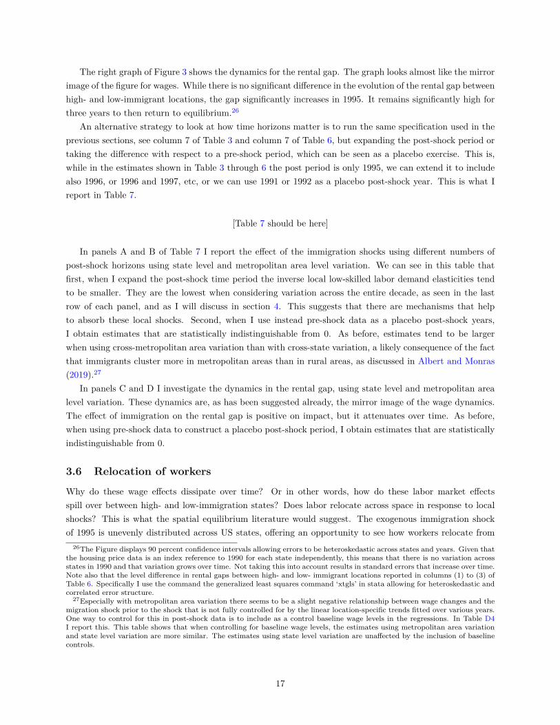
The right graph of Figure 3 shows the dynamics for the rental gap. The graph looks almost like the mirrorimage of the figure for wages. While there is no significant difference in the evolution of the rental gap betweenhigh- and low-immigrant locations, the gap significantly increases in 1995. It remains significantly high forthree years to then return to equilibrium.26

An alternative strategy to look at how time horizons matter is to run the same specification used in theprevious sections, see column 7 of Table 3 and column 7 of Table 6, but expanding the post-shock period ortaking the difference with respect to a pre-shock period, which can be seen as a placebo exercise. This is,while in the estimates shown in Table 3 through 6 the post period is only 1995, we can extend it to includealso 1996, or 1996 and 1997, etc, or we can use 1991 or 1992 as a placebo post-shock year. This is what Ireport in Table 7.


In panels A and B of Table 7 I report the effect of the immigration shocks using different numbers ofpost-shock horizons using state level and metropolitan area level variation. We can see in this table thatfirst, when I expand the post-shock time period the inverse local low-skilled labor demand elasticities tendto be smaller. They are the lowest when considering variation across the entire decade, as seen in the lastrow of each panel, and as I will discuss in section 4. This suggests that there are mechanisms that helpto absorb these local shocks. Second, when I use instead pre-shock data as a placebo post-shock years,I obtain estimates that are statistically indistinguishable from 0. As before, estimates tend to be largerwhen using cross-metropolitan area variation than with cross-state variation, a likely consequence of the factthat immigrants cluster more in metropolitan areas than in rural areas, as discussed in Albert and Monras(2019).27

In panels C and D I investigate the dynamics in the rental gap, using state level and metropolitan arealevel variation. These dynamics are, as has been suggested already, the mirror image of the wage dynamics.The effect of immigration on the rental gap is positive on impact, but it attenuates over time. As before,when using pre-shock data to construct a placebo post-shock period, I obtain estimates that are statisticallyindistinguishable from 0.

3.6 Relocation of workers

Why do these wage effects dissipate over time? Or in other words, how do these labor market effectsspill over between high- and low-immigration states? Does labor relocate across space in response to localshocks? This is what the spatial equilibrium literature would suggest. The exogenous immigration shockof 1995 is unevenly distributed across US states, offering an opportunity to see how workers relocate from

26The Figure displays 90 percent confidence intervals allowing errors to be heteroskedastic across states and years. Given thatthe housing price data is an index reference to 1990 for each state independently, this means that there is no variation acrossstates in 1990 and that variation grows over time. Not taking this into account results in standard errors that increase over time.Note also that the level difference in rental gaps between high- and low- immigrant locations reported in columns (1) to (3) ofTable 6. Specifically I use the command the generalized least squares command ‘xtgls’ in stata allowing for heteroskedastic andcorrelated error structure.

27Especially with metropolitan area variation there seems to be a slight negative relationship between wage changes and themigration shock prior to the shock that is not fully controlled for by the linear location-specific trends fitted over various years.One way to control for this in post-shock data is to include as a control baseline wage levels in the regressions. In Table D4I report this. This table shows that when controlling for baseline wage levels, the estimates using metropolitan area variationand state level variation are more similar. The estimates using state level variation are unaffected by the inclusion of baselinecontrols.

17

high-immigration locations to low-immigration locations when hit by an unexpected inflow of low-skilledworkers.28


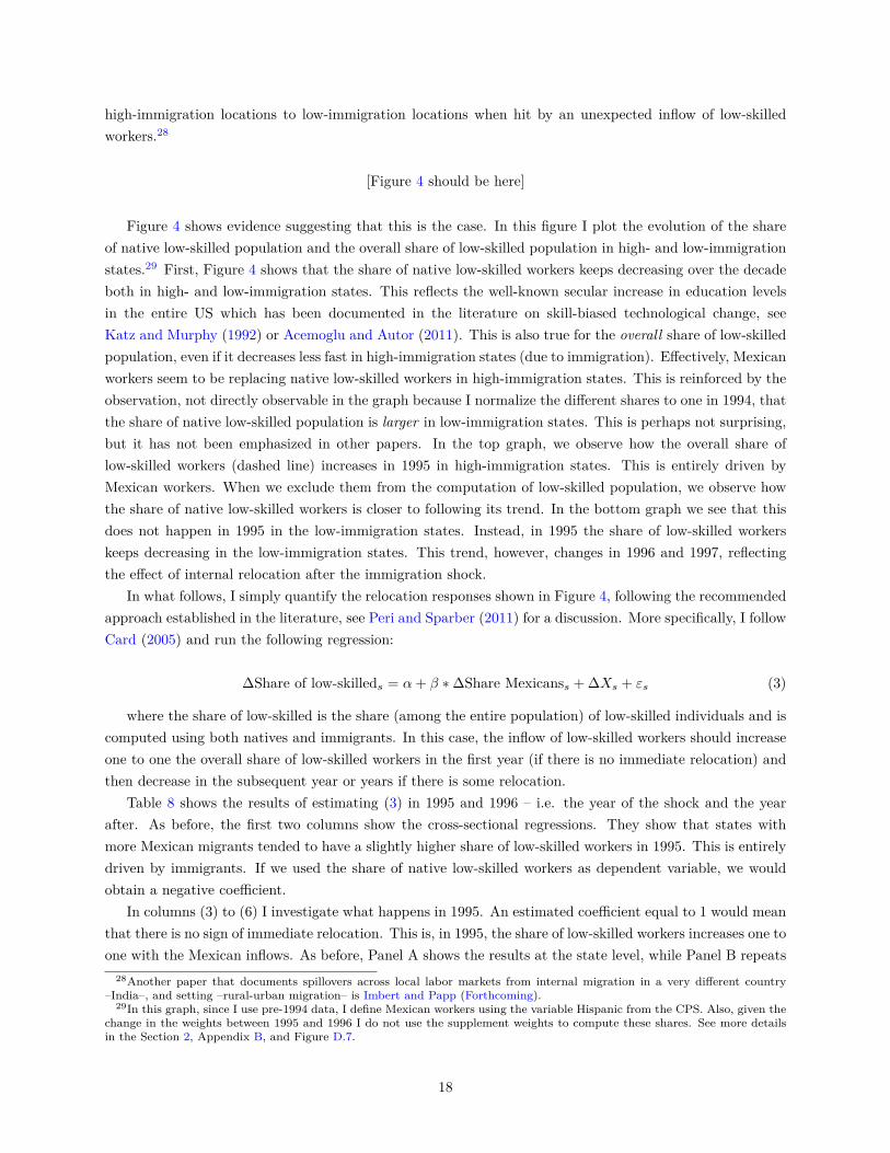
Figure 4 shows evidence suggesting that this is the case. In this figure I plot the evolution of the shareof native low-skilled population and the overall share of low-skilled population in high- and low-immigrationstates.29 First, Figure 4 shows that the share of native low-skilled workers keeps decreasing over the decadeboth in high- and low-immigration states. This reflects the well-known secular increase in education levelsin the entire US which has been documented in the literature on skill-biased technological change, seeKatz and Murphy (1992) or Acemoglu and Autor (2011). This is also true for the overall share of low-skilledpopulation, even if it decreases less fast in high-immigration states (due to immigration). Effectively, Mexicanworkers seem to be replacing native low-skilled workers in high-immigration states. This is reinforced by theobservation, not directly observable in the graph because I normalize the different shares to one in 1994, thatthe share of native low-skilled population is larger in low-immigration states. This is perhaps not surprising,but it has not been emphasized in other papers. In the top graph, we observe how the overall share oflow-skilled workers (dashed line) increases in 1995 in high-immigration states. This is entirely driven byMexican workers. When we exclude them from the computation of low-skilled population, we observe howthe share of native low-skilled workers is closer to following its trend. In the bottom graph we see that thisdoes not happen in 1995 in the low-immigration states. Instead, in 1995 the share of low-skilled workerskeeps decreasing in the low-immigration states. This trend, however, changes in 1996 and 1997, reflectingthe effect of internal relocation after the immigration shock.

In what follows, I simply quantify the relocation responses shown in Figure 4, following the recommendedapproach established in the literature, see Peri and Sparber (2011) for a discussion. More specifically, I followCard (2005) and run the following regression:

∆Share of low-skilleds = α+ β ∗∆Share Mexicanss + ∆Xs + εs (3)

where the share of low-skilled is the share (among the entire population) of low-skilled individuals and iscomputed using both natives and immigrants. In this case, the inflow of low-skilled workers should increaseone to one the overall share of low-skilled workers in the first year (if there is no immediate relocation) andthen decrease in the subsequent year or years if there is some relocation.

Table 8 shows the results of estimating (3) in 1995 and 1996 – i.e. the year of the shock and the yearafter. As before, the first two columns show the cross-sectional regressions. They show that states withmore Mexican migrants tended to have a slightly higher share of low-skilled workers in 1995. This is entirelydriven by immigrants. If we used the share of native low-skilled workers as dependent variable, we wouldobtain a negative coefficient.

In columns (3) to (6) I investigate what happens in 1995. An estimated coefficient equal to 1 would meanthat there is no sign of immediate relocation. This is, in 1995, the share of low-skilled workers increases one toone with the Mexican inflows. As before, Panel A shows the results at the state level, while Panel B repeats

28Another paper that documents spillovers across local labor markets from internal migration in a very different country–India–, and setting –rural-urban migration– is Imbert and Papp (Forthcoming).

29In this graph, since I use pre-1994 data, I define Mexican workers using the variable Hispanic from the CPS. Also, given thechange in the weights between 1995 and 1996 I do not use the supplement weights to compute these shares. See more detailsin the Section 2, Appendix B, and Figure D.7.

18

the exercise at the metropolitan area level. In column 3 I show that even with a simple OLS regression Iobtain a coefficient that is already close to 1 when using cross-state variation. Across-metropolitan areas thecoefficient is lower than 1, suggesting that there may be some interesting within state, urban-rural internalmigration that I do not explore in this paper. In column 4 I include controls and in column 5 I use an IVspecification. Coefficients stay quite constant when using cross-state variation and tend to increase whenusing cross-metropolitan areas variation. My preferred estimate is shown in column 6.30 There I show theestimate using an IV strategy and controlling for the change in native low-skilled population. This allowsfor different trends in the native low-skilled population across space. In this specification, I obtain a tightestimate very close to 1, both using cross-state and cross-metropolitan area variation. This estimate suggeststhat once we take into account state or metropolitan area specific trends, the unexpected inflow of Mexicanworkers in 1995 led to a one to one increase in the share of low-skilled population.


Columns 7 to 10 investigate what happened in 1996, one year after the unexpectedly large inflow ofMexicans that increased the share of low-skilled workers in the high-immigration states. We immediatelysee that with the OLS estimates we already obtain an estimate significantly smaller than one. The IVestimate, suggests, in fact, that the share of low-skilled workers almost reverts back to where it was beforethe unexpected inflow of Mexican workers. This is the case when I use cross-state variation and when I usecross-metropolitan area variation, although in the latter case, estimates are much more noisy. The negativecoefficients are evidence that there was some labor relocation taking place the year after the unexpectedlylarge inflow of Mexican workers of 1995 and is in line with Figure 4. This strong response can generate thewage dynamics previously discussed, something that becomes even more clear when I discuss the model insection 5.31

4 Longer-run effects of Mexican immigration

The fact that there is some relocation of low-skilled workers away from high-immigration states as a responseto a negative shock to wages and rental gaps, and convergence across space, makes it more difficult to evaluatethe longer-run effects of immigration on labor and housing market outcomes. Simply put, internal migrationgenerates spillovers between treatment and control units that tends to attenuate the estimated effect. Thereare a number of alternatives one can adopt to shed more light on the longer-run consequences of immigration.These can be divided between longer-run empirical comparisons and counterfactual wage and housing priceevolutions from a structural model. I present the empirical long-run results in this section, and move to thestructural modeling in sections 5 and 6.

4.1 Long-run identification strategy

To investigate the long-run impact of immigration across locations I use the following regression:30An alternative to this column is to run two separate regressions one using as dependent variable the share of low-skilled

population, and the other one using the share of native low-skilled population (where the estimate would show a 0). In orderto save some space I opted for just including the change in the share of native population as a control.

31There are various internal and international migration responses that could explain these internal migration patterns. Idiscuss them in detail in Appendix A.7.

19

∆00−90 ln ys = α+ β ∗ ∆00−90MexsNs,90

+ εs (4)

where ∆00−90 indicates the difference between 1990 and 2000 of the relevant variable. It is important tonote that, in this specification, I use the relative inflow of Mexican workers instead of the change in the sharebecause I consider the population at the beginning of the period to be the size of the relevant labor market.Given the population growth over the 90s in the United States, this strategy obtains a smaller estimate (inabsolute value) than using the change in the share of Mexican workers. Thus, the results shown in whatfollows are conservative estimates.32

This specification is very similar to the ones used in Card (2001) and especially Altonji and Card (1991).As mentioned before, the presumption that Mexicans may be choosing where to migrate within the USmotivated the construction of the networks instrument. The validity of the immigrant network instrumentrequires new inflows of Mexican workers to be strongly influenced by the past stock of Mexicans in the USand there are no spillovers across states. I report the results in Table 9, commented below. The exactformulation of the instrument follows equation 2 but applied to the ten year differences.

An alternative specification for investigating the long-run impact of immigration is used by Borjas (2003).He assumes that there are spillovers between geographic units and completely forgets about them in his mainspecifications. Instead, Borjas (2003) uses across-cohort or across-age (denoted by a) variation to study thelong-run effect of immigration. This is:

∆00−90 ln ya = α+ β ∗ ∆00−90MexaNa,90

+ εa (5)

The assumption in this case is that different age cohorts of potential migrants do not take into accountthe labor market outcomes of their own group when migrating. Under this assumption, an OLS regressionwould estimate the causal effect of immigration on outcomes ya if workers of different age groups are im-perfect substitutes. It is likely, however, that migrants at least in part, look at their relevant labor marketopportunities when deciding to migrate, and this includes any of their own characteristics, among whichexperience. This last concern also suggests that we must find a valid instrument for this regression so asto interpret the estimate causally. I build such an instrument based on the unexpectedly large inflow ofMexicans in 1995 and on the fact that the age distribution of Mexican immigrants was very constant overthe entire 1990-2000 decade, as shown in Figure D.2 in the Appendix. Specifically, I construct:33

Predicted migrantsa =2000∑j=1991

Mexican Migrants aged a at arrivalTotal Mexican arrivals ∗Mexj (6)

This is, I assign the inflow of Mexicans at year t using the age distribution of the entire decade to matchthe particular age cohort that receives the shock. If there are some years with an unexpectedly large inflow ofimmigrants and the age distribution of this inflow is not affected, then there will be some native cohorts withunexpectedly large competition. This is the nature of this IV. Given that the age distribution of Mexicanarrivals is tilted towards entry-level positions, this IV will rely on the evolution of labor market outcomes ofdifferent cohort entries observed in 2000 relative to the cohorts observed in 1990.

32In the previous short-run regressions, this distinction does not matter so much because the population growth in a givenyear is significantly less pronounced than over an entire decade. Note that without population growth, the two specificationsare identical.

33In the regression I use 46 age categories that include ages between 20 and 65 years old, both included. When looking athigh-skilled workers I use ages between 25 and 65, also both included.

20

As before, the first-stages are strong, as shown in Table D9 in the Appendix. The past importance ofMexicans in a location or age group is a good predictor of larger inflows over the 1990s.

4.2 Wages

Table 9 shows the empirical results of the effect of Mexican migration in the long-run on labor marketoutcomes. Each panel of this table is divided in three parts. The first one shows cross-state, the secondcross-metropolitan area, and the third, cross-age comparisons. Panel A shows the effect on low-skilled nativewages, while panel B shows the exact same regressions but using the change in high-skilled wages instead.Panels C and D report results on employment.

As in previous literature, across-location OLS estimates of Mexican inflows and wage changes are notstatistically different from zero, as can be seen in Panels A and B of Table 9. In column 2 and 4, Iinstrument the OLS regression with the immigration networks instrument. The coefficient becomes slightlymore negative, suggesting a long-run local labor demand elasticity of around -.3 when using cross-state andaround -.4 when using cross-metropolitan area variation. This is the slightly negative trend in high- relativeto low-immigration locations discussed in Figures 2 and 3 and is similar to previous studies. Note thatcolumns 1 to 4 simply follow the literature initiated by Altonji and Card (1991), but applying the regressionspecfically to Mexican immigrants. Columns 5 and 6 instead follows Borjas (2003). Like him, I find anegative estimate of around -.3 when using OLS (column 5). In column 6, I use the instrument proposed inequation 6. When instrumenting to take into account the possible selected immigration in particular yearsand selected return migration by Mexicans, I obtain an estimate of around -.53.


Panel B of Table 9 shows the exact same regressions as in the upper part but using the change of high-skilled wages instead of low-skilled. All the estimates in this part of the table are close to 0. In other words,Mexican immigration seems to have affected only low-skilled workers in the long-run. And among those, theones that suffered larger shocks when young, seem to have suffered more lasting consequences.

4.3 Employment

If there is some wage stickiness or some endogenous (intensive margin) labor supply response, part of theeffect of Mexican immigration over the decade may be observable in the employment rate. As with theshort-run estimates, I also analyze the effect of immigration on employment within locations and age groups.

Following Panels A and B, Panels C and D report the results for employment rates. Qualitatively theresults are almost identical across panels. Across-space high Mexican immigration locations experienceonly very small declines in the employment rate, both when comparing states and metropolitan areas.In columns 5 and 6 I report the cross-age regressions. These columns suggest that low-skilled Mexicanimmigration decreases employment rates of low-skilled natives substantially. Both in the OLS and in the IVspecifications a 10 percent immigration induced labor supply shock decreases employment rates by around6 or 7 percent. Very importantly too, when I repeat the exercise using high-skilled native employment ratesI obtain an IV estimate closely at 0.

This evidence suggests that part of the effect of immigration on labor market outcomes is observedon wages and part on employment rates. In both cases, however, estimates are lower when comparing

21

across space than when comparing across-age or experience groups. This is in-line with and complementsprior literature. Overall, I take this as evidence that labor market effects dissipate to a large extent acrossspace, but that there are particular cohorts of low-skilled workers – those that enter the labor market inhigh-immigration years – that are affected over longer time horizons.

4.4 Housing market

The third piece of longer-run evidence is on housing market prices. For this I can only use across-spacecomparisons. Mexican workers may affect housing prices and rents in a number of different ways and, alsoin this case, time horizons may matter. For instance, as explained in Saiz and Wachter (2011) and in Sa(2015), immigrants may increase the demand for housing, thus putting pressure on housing prices and rents.This is likely to happen over short time horizons, which is what I showed in Section 3.4. Over longer timehorizons there are other forces. First, maybe natives prefer to live in different neighborhoods or locationsas a response to immigrant inflows. Depending on this response, this may lower the demand for housing inhigh-immigrant locations. Second, immigrants may affect the quality of local public goods, thus reducingthe amenity value of living in certain locations. And third, maybe they affect the quality of housing. BothSaiz and Wachter (2011) and Sa (2015) concentrate on these three mechanisms and suggest that native’spreferences for not living with immigrants is the main driver of the negative relation between housing pricesand rents and immigrant inflows at the neighborhood level that they document.

However, there may be other important reasons as well. Something particular about Mexican low-skilledworkers is that they disproportionately enter the construction sector, potentially affecting the constructioncosts. In turn, given that labor costs account for the bulk of construction costs as documented in Gyourkoand Saiz (2006), this may affect housing prices. I show that this possibility is very much in line with theevidence on Mexican migration over the 90s. In Table D10 in the Appendix, further discussed in AppendixSection A.9, I show that around half of Mexicans enter the construction sector, fully displacing natives inthat sector, which is something that can also be seen in the summary statistics data presented in Table 1.This leads to a very significant reduction of native wages in the construction sector in high- relative to low-immigration locations. Moreover, Mexicans earn, on average, lower wages than natives, further decreasingconstruction costs.

Thus, there are a number of forces that may lead housing prices to decline in high Mexican-immigrationlocations relative to low Mexican-immigrant locations. These may prevail over the short-run pressure onrental prices, even if this pressure spills-over to selling prices so that the gap between the two does not persistover time as shown in section 3.5, Figure 3.


Using longer-run across-space comparisons I show evidence that is in line with these ideas. When com-paring changes in the housing price index or in rental prices between 1990 and 2000 across locations we seethat locations that over the 90s received large inflows of Mexican workers experienced declines in housingand rental prices. These results are shown in Table 10. Using both cross-state and cross-metropolitan areavariation, the IV estimates in columns 2 and 4 suggest that higher inflows of Mexican immigrants led to bothlower housing prices and lower rental prices, with and elasticity of around -1. The drop in both cases is ofthe same magnitude and slightly larger than the OLS estimate presented in columns 1 and 3, making thechange in the rent gap, shown in columns 5 and 6, statistically indistinguishable from 0.

22

To assess whether these results may be driven by a cost reduction in construction I show in AppendixA.10 that in a perfectly competitive construction sector, house price declines can be approximated by thecost share of labor in the sector times the local labor demand elasticity adjusted for composition effects.34

This would imply, as illustrated in Appendix A.10, an elasticity of around -0.84, which is in line with theestimates in Table 10. A second corroborating piece of evidence is that this reduction in housing pricesshould lead to an increase in construction according to the price elasticity of the local demand for housing.In Appendix A.10, I show data on new construction across states that suggests that this elasticity is between-0.3 and -0.4, in line with Hanushek and Quigley (1980) and Mayo (1981).

Taken together, the evidence presented in Figure 3, Table 10, Table D10, and Appendix A.10 shows thatMexican migration created a decline in housing prices and rents over the 90s, to a large extent driven bythe impact of Mexican migration on the construction sector, but that at the same time, unexpectedly largeinflows like the one occurring right after the Mexican Peso crisis, temporarily increase rental prices, sinceMexicans disproportionately use this housing market.

4.5 Relocation

The final piece of evidence using 1990 and 2000 Census data is on long-run spatial relocation. I stressedbefore that over the short-run there is an important internal migration response to the unexpectedly largeinflow of Mexican workers in 1995 which helps local shocks to dissipate spatially. There is some literature,however, that suggests that internal migration does not seem to respond strongly using longer time horizons.To reconcile these results it is important to realize that there may be different ways in which expectedand unexpected immigrant flows are absorbed. Unexpected inflows put pressure on both labor and housingmarkets, and as a consequence internal migration responds. When inflows are expected, as was the casewith most of the years with Mexican migration during the 90s, local technologies or capital may adjust tohelp absorb labor supply shocks. The more local technologies adjust, the less internal migration is needed toequilibrate the value of living across local labor markets. I use these ideas when discussing counterfactualsin Section 6.


Table 11 shows the results. The first three columns show that in 1980 Mexicans entered states wherethe share of low-skilled workers was lower. Over the following two decades, the share of low-skilled workersincreased more in initially high-immigration states, as can be seen in columns 2 and 3. Column 4 is yetanother way of looking at the first-stage regression of the immigration networks instrument used in theimmigration literature. We observe that the importance of Mexicans in the low-skilled labor force in 1980 isa good predictor of where the share of Mexicans would increase more during the 90s. This is the instrumentused in column 6 and 8. Columns 5 and 6 estimate the relocation equation 3. The OLS and IV estimates ofcolumns 5 and 6 suggest that for every low-skilled Mexican entering a high-immigration state, the state gains0.8 low-skilled workers. This estimate decreases to 0.6 when controlling for the 1980 distribution of low-skilled workers in the US, which effectly allows for different trends to depend on the baseline importance of

34I estimate the local labor demand elsticity to be around -1. Gyourko and Saiz (2006) argue that the construction sectoris well approximated by a perfectly competitive model and that the cost share of labor is at least 60 percent. Note also thatMexican inflows can lead to a decline in wages for two reasons. One, a direct effect of the shock on native wages, and, two, ifMexican workers earn on average less than natives as shown in Table 1, they can lead to a further reduction in average wagesdue to a composition effect. The composition adjustment is given by the difference in native and Mexican wages divided by theaverage wage. In the data this is typically around 40 percent.

23

Mexican workers. This is consistent with the estimates in Wozniak and Murray (2012). This is also certainlyconsistent with Figure 4 and with the story that while high-immigration locations absorb an important shareof low-skilled Mexicans by increasing the use of this factor locally, unexpected shocks can be accommodatedthrough internal migration. Monras (2018) suggests that this is a consequence of reduced in-migration intoshocked locations which explains the fast response, but CPS data is limited to explore this further in thispaper.35 As before, results using cross-state (Panel A) and cross-metropolitan area (Panel B) variationare very similar. If anything, cross-metropolitan area variation suggests a more important role for internalmigration than cross-state variation.

5 A Structural model of the local adjustment to immigration

While it is possible to evaluate the short-run effects using a clear natural experiment, spillovers acrosslocations due to labor relocation makes it more difficult to evaluate longer-run effects using across-spacecomparisons. Across-age comparisons help to overcome some of the limitations of the spatial reallocation,however, they are not useful to think about the general equilibrium, nor for some outcomes like housingprices. For this reason, I introduce in this section a spatial equilibrium model that I then bring to the data.

In the very short-run, each local labor market, in this case states or metropolitan areas, is closed, sostandard models of the aggregate labor market apply (see the canonical model discussed in Acemoglu andAutor (2011) or Katz and Murphy (1992)). In the longer-run, internal migration flows link the variouslocal labor markets, spreading local shocks to the rest of the economy, either through affecting local wagesor local housing prices. Standard models in the spatial economics literature in the spirit of Rosen (1974)and Roback (1982) are suited to analyzing the long-run, once adjustment has taken place (see also Glaeser(2008), Moretti (2011) or Allen and Arkolakis (2014)). Fewer models in this literature are suited to studyingthe transition dynamics.

Two seminal contributions introduced transition dynamics into a model with many regions: Blanchardand Katz (1992) and Topel (1986). For instance, Blanchard and Katz (1992) report that wages seem toconverge spatially after around 8 years, while unemployment rates converge faster. In the estimation of theirmodel, they rely mainly on time series variation, although they also use Bartik (1991) type instruments likesubsequent literature (see Diamond (2015) and Notowidigdo (2013)). They do not microfound, however, themigration decisions.

The seminal contribution of Kennan and Walker (2011) introduces a dynamic micro-founded migrationmodel. The multiple locations and migration histories that workers can choose makes this problem particu-larly hard. Kennan and Walker simplify in two respects. First, they only take into account a subset of thepossible choices of workers. Second, their model is, in nature, partial equilibrium. They do not model therest of the economy and the interactions between the different states as I do in what follows. In exchange, inthe model that I present here I simplify the location decision by allowing only a fraction of the population tomove, which is the empirical relevant special case of the discrete choice model presented in Monras (2018).Relative to Monras (2018) I allow for different types of housing and different skill types.

The model has S regions representing US states or metropolitan areas. There is a single final consumptiongood that is freely traded across regions, at no cost. It is relatively simple to introduce trade in this contextsince it simply determines a particular price index for tradable goods prevailing in each local economy.Assuming free trade equalizes this price index of tradable goods to one. I leave costly trade outside the

35The question on the residence in the previous year is not asked in the CPS in 1995.

24

model for simplicity.36

Workers can be either high- or low-skilled. They are the two factors of production of a representative firmin every local market. The only difference between firms in different locations is the underlying productivityof each factor and a Hicks-neutral technology parameter. For simplicity, I assume in this model that theHicks-neutral technological parameter is not affected by international or internal migration. This is perhapsan unrealistic assumption, since many papers in urban economics have estimated that local productivityis increasing in population (Combes and Gobillon, 2014), with an elasticity of almost 5 percent. In thecontext of the model, including this technological adjustment would lead to a uniform increase in the wagelevels of each factor type if the location gains population. However, given that the most important aspectis how immigrants affect skill-specific types and that the implied elasticity of substitution between those isestimated to be around one, considering endogenous agglomeration forces is unlikely to be quantitativelyvery important in this context.

Labor markets are perfectly competitive. Every worker lives in either a rented or an owned housing unit.Rented and owned housing units are treated as two separate housing services that satisfy worker’s demandsfor shelter. Workers live for infinitely many periods and are small relative to the labor market.

The timing of the model is as follows. At the beginning of each period, workers observe amenity levels,wages, and housing prices in every location. A fraction of them are allowed to move across locations and getan idiosyncratic taste draw from a known distribution over potential destinations and types of housing. Thenon-movers get a draw for the different types of housing within the location. Based on this, everyone decideswhere to relocate. Hence, by the end of the period, there is a new distribution of people across locationsand housing market types. In the following period, this new distribution of people determines new wagesand new housing prices at the local level through market clearing, something that I label as the short-runequilibrium. Once these are determined, we are at the beginning of the new period.

The long-run equilibrium is defined as a short-run equilibrium with zero net flows of workers acrosslocations. Hence, in the long-run the the distribution across locations of workers of each type is stable. Thelong-run equilibrium coincides with the equilibrium in standard spatial equilibrium models, where indirectutility of the marginal mover is equalized across space. The main difference between this model and standardquantitative static spatial equilibrium models is that taste heterogeneity – modeled with the idiosyncratictaste draws – shapes the flows of workers across locations instead of directly its final distribution. In thismodel’s long-run equilibrium there are always positive gross flows of workers between any two locations thatexactly cancel each other out.

To summarize, in the model there are essentially four types of workers: high- and low-skilled workers thateither rent or buy housing units. High- and low-skilled workers are imperfect substitutes in production, butthey may be competing for housing units in either the rental or home-ownership markets. “Sticky” mobility– from rental to home owned units and internal migration – links the experiences of the various workersacross space, local housing, and labor markets. This sticky mobility is what generates the dynamics in bothlocal labor and housing markets. It crucially depends on two elements: the equilibrium internal mobility(which I take from 1990 Census data) and the responses to shocks.

5.1 Indirect Utility Function

Workers of each skill type earn the market wage of the location they reside in. Since there is only onetradable good, housing, and no savings, they spend all of their wage on this good and on housing. In what

36Adding a richer trade model would simply create a location-specific price index for tradable goods in each local market.

25

follows I present the indirect utility and location choice part of the model only for native low-skilled workers.The model for high-skilled workers is exactly the same except that the relevant wages are the high-skilledwages (hs in the empirical section). When I need to distinguish Mexican and native workers, or nativeworkers of different skills, I follow the notation from the previous sections. This is, I denote by Ns nativelow-skilled workers, by Ls = Mexs + Ns all low-skilled workers, and by Hs high-skilled workers. Mexs

denotes Mexican low-skilled workers who just arrived to the US. After one period in the US they behave likelow-skilled natives.

Indirect utility of low-skilled workers who consider s′(r) as a potential residential choice is given by thelocal wage ws′ , the amenities As′(r) – which are also skill specific and depend on the housing market choice–,the housing price pt,s′(r) that they will face at destination – where r determines if it is a rental unit or anowned unit –, the continuation value of being at s′, and the idiosyncratic draw they get for location s′ andhousing market type r:37

lnV it,s′(r) = lnVt,s′(r) + εit,s′(r) = lnAs′(r) + lnwt,s′ − α ln pt,s′(r) + βEt lnVt+1,s′ + εit,s′(r) (7)

Note that the indirect utility has a common component to all (low-skilled) workers in housing markettype r and location s′, given by lnVt,s′(r), which is the value of living in s′(r), and an idiosyncratic componentεit,s′(r) specific to each worker.38 Intuitively, the variance of ε determines whether the common componentor the idiosyncratic component has a higher weight in this decision. Finally, α is the share of spending thatgoes into housing. While this may, in principle, vary across local labor markets and between home-ownersand renters, it is fairly stable in the data at around 25 percent of total income (Davis and Ortalo-Magne,2011). For simplicity I make this a common constant across locations and types of household.

5.2 Location Choice

Each period, workers decide where they want to reside, given the indirect utility they get in each place. Thatis, each worker i maximizes:

maxs′∈S,r∈R

{lnVt,s′(r) + εit,s′(r)} (8)

The general solution to this maximization problem gives the probability that an individual i residing ins moves to s′(r) in housing market type r:

πit,s,s′(r) = πt,s,s′(r)(Vt,s′(r); s′ ∈ S, r ∈ R) (9)

As mentioned before, I further assume that only a fraction η of workers decide on cross-space relocationeach period, while the other fraction can only change apartment types within a location. This fraction η

can be endogenized. I do this in Monras (2018) and show that it is empirically not very relevant.39 Thisparameter η is important for the quantitative exercise, since the model would otherwise over-predict yearlybilateral mobility in the absence of shocks. It plays a very similar role to fixed costs of moving – but

37This indirect utility function can be easily derived from a Cobb-Douglass utility function with two goods, housing and atradable good. More quantity of housing can be re-interpreted as higher quality housing (or bigger apartments). See appendixC.1.

38Like in many papers in the spatial equilibrium literature I view this parameter ε as capturing taste heterogeneity for livingin different locations. Other papers have used this idiosyncratic shock to study unobserved skill heterogeneity, see Morten andBryan (Forthcoming). I abstract from this view of the idiosyncratic variable in this paper.

39In order to identify the parameters of an endogeneized η I need data on both in- and out-migration rate responses to localshocks. This is not avalable in the CPS for 1995. I refer the reader to Monras (2018).

26

introducing it in this way makes the model much more tractable. The non-movers do decide, however, whattype of housing market to be in the following period.40

By the law of large numbers we can then use equation (9) to obtain the flow of people between s ands′(r). I also assume that ε is drawn from a nested logit extreme value distributed.41 This has the niceproperty that the difference in ε is also extreme value distributed resulting in a closed form solution for theprobability of an individual moving from s to s′ and entering housing market r. We can use this propertyto write the bilateral flows as follows:

Πt,s,s′(r) = ηNt,sV

1/λt,s′∑j V

1/λt,j

V1/γt,s′(r)∑r V

1/γt,s′(r)

, for s 6= s′ (10)

where λ and γ govern the variance of the error term, and where Vt,s′ is the expected value of living in s′

on either a rental unit or on an owned unit: Vt,s′ = (∑r V

1/γt,s′(r))

1/γ . This expected value is obtained fromthe distributional assumption on ε.42 This equation says that a fraction ηV

1/λt,s′ /

∑j V

1/λt,j of workers in s

will move to s′ – η is the fraction of workers in s that consider relocating, and among those, the fractionV

1/λt,s′ /

∑j V

1/λt,j decides on s′. Among the movers towards s′, a fraction V 1/γ

t,s′(r)/∑r V

1/γt,s′(r) will enter housing

market r ∈ {rental, owner}.Furthermore, the nested logit error term results in a simple equation for the evolution of the common

component of the value of living in each location’s housing market r:

Vt,s′(r) = (As′(r)wt,s′

pαt,s′(r))V βηt+1V

β(1−η)t+1,s′ (11)

where Vt+1 = (∑j V

1/λt+1,j)λ is the overall value of the economy for the low-skilled workers. This equation

means that the value of living in location s′ and housing market r is given by the value of wages and amenitiesrelative to housing costs (weighted by the share of income devoted to housing α) and the value of being inthat location in the future, discounted by β. In turn, the value of living in location s′ in the followingperiod is a weighted average of being a mover in the following period and searching for a new destinationand staying put in location s′.

Another of the key aspects of the model is that it delivers simple and intuitive population dynamicsacross local labor and housing markets. Integrating over destinations using the definition of Πt,s,s′(r) weobtain that:

Nt+1,s′(r) = η(Vt,s′

Vt)1/λ(

Vt,s′(r)

Vt,s′)1/γNt + (1− η)(

Vt,s′(r)

Vt,s′)1/γNt,s′ (12)

This equation means that the number of people in location s′ and housing type r is a weighted averagebetween the amount of people in this location in the previous period times the value of housing market type

40It is also easy to induce more “stickiness” in the housing market by allowing only a (potentially endogenous) fraction ofresidents to switch housing markets. Given that in the data housing dynamics evolve relatively quick and that it is probablynot very costly to move to a new apartment within a location, I do not include this extra “stickiness”. Appendix C.5 discussesthese issues with more detail.

41Two classes of distributions admit close form solutions. One is extreme value distributions and the other is a uniformdistribution. See Moretti (2011) for an example of the latter.

42It is relatively simple to introduce more flexibility into the model to explain the data even better. For example, one can have“weights” such that instead of (V 1/γ

t,s′(r))(∑

rV

1/γt,s′(r)) we have (νrV 1/γ

t,s′(r))/(∑

rνrV

1/γt,s′(r)) to capture why it is more common to

move to a particular housing market (when arriving into a city), for example the rental market, than to another. Similarly, theremay be some locations that attract a disproportionate share of movers (beyond what is captured already by this model), whichcould be accommodated with weights in the upper nest. I abstract from this richness since it is not of first order importanceto explain the data.

27

r, the second term, and the share of movers that decide to move into location s′ using housing market typer, the first term.

Equations 11 and 12 define a dynamic system of two equations and two unknowns for each of the locationsand housing market types in the economy for low-skilled workers.43 The equations depend on local prices,i.e. wages and housing markets, which are determined locally as I explain below. A similar set of equationsapplies to high-skilled workers. Hence, I have four types in the economy: high-skilled owners, high-skilledrentes, low-skilled owners, and low-skilled renters. The interaction between the labor and housing marketdefines the value in each location for the four worker types.

Under these assumptions one can prove that the derivative of (net) in-migration rates in s with respectto (log) wages in s is approximately 1

1−β(1−η)1λIsNs

, where IsNs

is the in-migration rate (around 3 to 5 percentin US data, depending on the geographic unit of analysis), where I drop the time subscript t since this“response” does not depend on the time period, but rather to an unexpected change in wages. This can beexpressed more concisely as follows:

Proposition 1. If εis(r) are iid and follow a nested logit distribution with shape parameters λ and γ then,in the environment defined by the model, we have that:

1. ∂(lnNs)/∂ lnws ≈ 11−β(1−η)

1λIsNs

Proof. See Appendix C.2.

This is the first key elasticity of the model. It captures how much internal migration reacts to local shocks.Above I have implicitly estimated this elasticity by estimating the response of the share of low-skilled workersto the Mexican inflow. See section 3.6.

5.3 Production Function and Labor Market

The production function is given by a perfectly competitive representative firm producing according to:

Qs = Bs[θsHρs + (1− θs)Lρs ]1/ρ (13)

where Ls = Ns + Mexs is low-skilled labor (Mexicans plus natives) and Hs is high-skilled labor. θs

represents the different weights that the two factors have in the production function, while ρ governs theelasticity of substitution between low- and high-skilled workers. Bs is Total Factor Productivity (TFP) ineach state. θs are factor augmenting technologies, as in Acemoglu and Autor (2011).44 Firms do not takeinto account the future since they can adjust factor inputs instantaneously conditional on the factors thatare available in location s.

The marginal product of low-skilled workers is:

ws = p̃s(1− θs)Bσ−1σ

s Q1σs L

−1σs (14)

where σ = 1/(1− ρ) is the elasticity of substitution between high- and low-skilled workers and p̃s is theprice of the good. This defines the labor demand curve. We obtain a similar equation for the high-skilled.

43This formulation is quite flexible to introducing different types of assumptions, and in particular, different degrees of“stickiness”. For instance, it is easy to accommodate the idea that only a fraction η̃ of the population within a location may beconsidering to switch from a rental unit to an owned unit. I discuss this in more detail in Appendix C.5.

44See also Card and Lewis (2007), Lewis (2012), and more recently Clemens et al. (2018).

28

Note that we can normalize p̃s = 1. Free trade will guarantee that prices are the same across regions.45

We can also obtain the relative demand for labor by dividing the demands for each factor type. From therelative demand for labor equation we obtain a simple estimating equation that allows to recover σ fromimmigrant shocks:46

∆ ln wshs

= ∆ ln 1− θsθs

− 1σ

∆MexsNs

− 1σ

∆ ln NsHs

Note that this is the estimation equation introduced in Section 3.2 and estimated in Table 4.47

5.4 Housing market

The housing market consists of rental units and owned units. There is an elastic supply of housing thatcreates a positive relationship between the price of housing market r and the amount of people living inmarket r in each location, governed in Equation 15 by parameter φs. I also allow for a indirect effectof Mexican migration on housing prices (ψ in the equation), which I already estimated using long-runcomparisons in Section 4.4. This indirect effect captures the fact that many Mexicans, as discussed above,work in construction and lower the costs of both maintenance and new building construction. The indirecteffect also captures potential neighborhood spillovers. Some natives might like or dislike living near Mexicanimmigrants, something that I capture in a reduced form fashion. Thus, I assume that:

ln ps(r) = χs(r) + φs lnNs(r) + ψMexsNs

(15)

This is a reduced form equation that can be microfounded (see Saiz (2010)). The relationship betweenhousing markets r and r′ is given by the demand for housing, that arbitrages away potential differences inthe price of housing in different markets. In this equation φs captures the housing supply elasticity and χs(r)is the productivity of location s in producing housing of type r. Potentially, the housing supply elasticity isspecific to each location: Saiz (2010) provides one estimate for each metropolitan area.

Note that, with this specification, Mexican immigrants may affect differently the rental and ownershipmarkets if Mexican arrivals disproportionately enter the rental market, as was discussed in Table 1. To obtainan estimation equation close to what I used before we only need to take first differences from equation 15:

∆ lnps(r)

ps(r′)=

χs(r)

χs(r′)+ φs∆ lnNs(r) ≈ χ+ φs∆

MexsNs(r)

(16)

where I have assumed that all Mexican entrants into location s enter the rental market r and none entersthe home ownership market r′. Note that this is very close to the equation estimated in Section 3.4.48

5.5 Equilibrium

The definition of the equilibrium has two parts. I start by defining the equilibrium in the short-run. Itsatisfies three conditions. First, given the amenity levels, wages, and housing prices in each location, workers

45Costly trade would result in p̃s being specific to each location. In this alternative, p̃s would be a function of prices andworkers in each location and transport costs.

46From the relative demand for labor: ln wshs

= ln 1−θsθs

− 1σMexsNs

− 1σ

ln NsHs

, it is easy to derive the expression in changesshown below.

47See a longer discussion of this derivation in Borjas and Monras (2017) or in Dustmann et al. (2013).48The only difference is in the denominator, where I used the amount of low-skilled workers instead of the amount of renters

in the local economy. The two are quantitatively similar. I have used the amount of low-skilled workers in order to use thesame specification that I use for the labor market.

29

maximize their utility and decide where to live. Second, firms take as given the productivity Bs, theproductivity of each factor θs and factor prices in each location to maximize profits. Finally, labor andhousing markets clear in each location. This equates the supply and the demand for labor and housing anddetermines the wage and housing prices in every local labor market. More formally:

Definition I. A short-run equilibrium is defined by the following decisions:

1. Given {Als(r), Ahs(r), ws, hs, ps(r)}∀s∈S,r∈R, consumers maximize utility and location choice

2. Given {θs, Bs, σ, ws, hs}∀s∈S, firms maximize profits

3. Labor and housing markets clear in each s ∈ S so that {ws, hs, ps(r)} are determined

We can define the long-run equilibrium by adding another condition. In words, I say the economy is ina long-run equilibrium when bilateral flows of people of each skill type are equalized between regions.

Definition II. Given {θs, Bs, σ, Als, Ahs}s∈S, a long-run equilibrium is defined as a short-run equilibriumwith constant population within locations and housing markets. This is:

Ns,s′(r),t+1 = Ns,s′(r),t and Hs,s′(r),t+1 = Hs,s′(r),t, ∀s, s′ ∈ S and r ∈ R

Note that in the definition above, Mexican low-skilled workers do no seem to appear anywhere. I distin-guish between Mexicans and native or non-Mexican low-skilled workers only when Mexicans arrive to theUS unexpectedly. Once in the US, Mexican workers behave like natives.

5.6 Properties of the model

Only a share η of workers considers relocating each period. This implies that, depending on the size of thelocal shock and the sensitivity of workers to local shocks, relocation may take some time to materialize. Inthe long-run, in the absence of changes in the location specific variables, the economy converges to a situationin which the marginal worker is indifferent across locations and where factor prices, net of amenities percapita, are equalized across locations. Initial conditions and labor flows determine the size of each locationand the relative size of each skill in each location, determining the long-run equilibrium. In this long-runequilibrium there are still positive flows of internal migrants between the different regions. Net flows are,however, zero.

When the steady state receives an unexpected shock then the economy changes and reaches a newsteady state. The speed of convergence crucially depends on the relative importance that workers give toidiosyncratic tastes versus working conditions, governed by the variance of ε. If this variance is larger, thenidiosyncratic tastes become more important, while if it is zero, only labor market conditions matter andadjustment takes place instantaneously.

The case of interest for the current paper is an unexpected increase in the size of the low-skilled laborforce in location s due to Mexican immigration. Furthermore, I assume that all Mexicans enter the rentalmarket. In this case, the increase in Ls(r) driven by the Mexican inflows instantaneously puts pressure onwages of low-skilled workers and rental prices. This makes location s attractive to high-skilled workers, whileit makes it less attractive for low-skilled workers in s. Similarly it makes housing market r less attractivethan r′. Thus, some high-skilled workers move towards s while some low-skilled workers move away froms, and some workers within and across locations move from rental units to home-owned units. We cansummarize this process as follows:

30

Proposition 2. An (unexpected) increase in Ls(r) in s(r) leads to: a) an instantaneous decrease in ws, b)an instantaneous increase in hs, c) an instantaneous increase in the relative price of housing market r, d) arelocation of low-skilled workers away from s, e) a relocation of high-skilled workers toward s, f) a relocationof households from housing market r to r′, g) a gradual convergence of indirect utility across regions, and h)a gradual convergence in the rental and home-ownership markets.

Proof. See Appendix C.3.

6 Estimation and Counterfactuals

To bring this model to the data we need essentially two sets of moments. First, to obtain dynamics thatresemble what we observe in the data we need to estimate the key elasticities governing the response of thelabor and housing markets to unexpected inflows of workers. This is precisely the exercise I did in the firstpart of the paper using the unexpectedly large inflow of Mexicans following the Peso Crisis.

Second, in order to explain the levels of the various labor and housing market variables we need estimatesof the fundamentals in the economy. These are essentially the amenity levels – which I allow to be location,skill, and housing market specific –, the housing market constants – in some locations building may be moreexpensive or difficult –, the underlying productivity in each location, and the equilibrium internal migrationrate. To estimate these various fundamentals, I assume that the economy is in long-run spatial equilibriumin 1990 and use the structure of the model to exactly explain the data in that year.

Combining the baseline fundamentals and the key elasticities with the Mexican flows over the 1990s I canthen use the model to predict wage, housing price, and internal migration dynamics throughout the decade.

6.1 Estimates of the fundamentals in the economy

In this subsection I explain how I bring the model to match 1990 US Census data, using as before theequations for low-skilled workers. Similar equations apply for the high-skilled.49 The first task is to obtainthe initial conditions of the dynamic system defined by equations 11 and 12. For this, all I need to do is toimpose that Vt+1,s(r) = Vt,s(r) and Nt+1,s(r) = Nt,s(r). This is:

Ns(r) = η(VsV

)1/λ(Vs(r)

Vs)1/γN + (1− η)(

Vs(r)

Vs)1/γNs (17)

Vs(r) = (As(r)ws

pαs(r))V βηV β(1−η)

s (18)

where V = (∑j V

1/λj )λ and Vs = (

∑r V

1/γs(r) )γ .

From the population dynamics equation we obtain a number of interesting relationships between locationvaluations and populations that make the model particularly tractable. First, it is easy to show that Ns

N =(VsV )1/λ.50 This relationship simply states that the fraction of workers in a location reflects the value of livingin that location relative to the value of living in other locations, with an elasticity λ that is governed by theresponse of internal migration to local shocks, previously estimated.

49It is not important if I match 1990 US Census data or 1980 US Census data since there is a tight relationship in thecross-section between wage and population levels of the various skill groups and, hence, leading to similar estimates of theproductivity and amenity parameters.

50Aggregating Ns(r) over r we have: Ns = η∑

r(VsV

)1/λ(Vs(r)Vs

)1/γN + (1 − η)∑

r(Vs(r)Vs

)1/γNs = η(VsV

)1/λN + (1 − η)Ns.

31

It is also easy to show that in the long-run: Ns(r)N = (VsV )1/λ(Vs(r)

Vs)1/γ , i.e. the share of workers living in

housing market r in location s is driven by the share of value of s relative to the rest of the economy timesthe share of value of housing market type r in the location s, with an elasticity governed by γ which is theresponse of housing prices in market r relative to market r′, also estimated before. From these conditionswe can back out the amenity levels which are given by the following expression, as shown in Appendix C.4:

As(r) = As′(r)(NsNs′

)λ(1−β(1−η))−γ(Ns(r)

Ns′(r))γws

′

ws(ps(r)

ps′(r))α (19)

Note that with equation 19 we can express all the amenity levels across all locations and housing markettypes just in terms of amenities in one particular housing market in one location, this is, for example, interms of A1(1) which we can normalize to 1. Thus, from the long-run equilibrium we can back out the levelof amenities that exactly rationalizes the distribution of prices and workers observed in the data. Recentliterature usually refers to this exercise as inverting the model (Redding and Rossi-Hansberg, 2018).

In order to obtain the housing market prices and wages in counterfactual scenarios we also need all thetechnology parameters which in the model were presented as Bs, θs, χs(r), and φs. θs is the Cobb-Douglasweight of low-skilled labor prevailing in location s. This is obtained from the relative wage bill in thelocation.51 Given θs, it is easy to obtain Bs, which is the level of productivity or TFP in location s, fromcomparing the total output produced given the production function without the Bs term to the total wagebill, under the assumption that the representative firm in location s has 0 profits.52

In order to obtain χs(r) and φs I combine Saiz (2010) estimates of housing supply elasticities with thefact that I observe population levels and prices in each housing market type r. Using this information intoequation 15 allows me to recover χs(r), if I know ψ. To estimate ψ I use the long-run effect of Mexicanmigration on housing prices estimated in section 4.4.

Given these initial conditions, it is also easy to use the steady state conditions to obtain the finaldistribution of people across space and housing markets given the fundamentals and the total amount ofworkers in the economy. Computationally, this is useful in order to check that the dynamics bring theeconomy from the initial conditions to the new long-run steady-state.

Note that with these estimates, which are the initial conditions of the dynamic system, it is easy tocharacterize the dynamics using equations 11 and 12. This fully determines the evolution of the economy.Moreover, these estimates deliver a number of sensible cross-location relationships.53

6.2 Key Elasticities: Labor and Housing Markets

There are three key labor market moments, which I implicitly estimated using the unexpected immigrantshock. In this subsection I just make more explicit how we can recover the relevant model estimates fromthe IV regressions presented before.

In order to obtain an estimate of σ we can use the relative demand for labor. From it, as I explainedabove in section 5.3 we can easily derive the following equation:

∆ ln wshs

= ∆ ln 1− θsθs

− 1σ

∆MexsNs

− 1σ

∆ ln NsHs

51More specifically, θs = 1/(1 + wsLs/hsHS).52More specifically, Bs = [θsHρ

s + (1 − θs)Lρs ]1/ρ/(wsLs + hsHS)53In Figures D.8 and D.9 in the Appendix, I show that there is a strong correlation between the share of high-skilled workers

in a location and the implied θ from the estimation. Similarly, I show that both the wage of high- and low-skilled workers isstrongly related to the estimated underlying productivity.

32

This is the estimation equation used in Table 4, where I obtained an estimate of σ ≈ 1.The second key elasticity is the internal migration response to local shocks. Obtaining λ from the

instrumental variable estimates previously shown is less straightforward than for wages. This is because Ifollow the literature in estimating mobility as a response to Mexican inflows, instead of estimating it relativeto wage changes, or location value changes, which is what the model requires. It is, however, possible torecover λ from the estimates presented already. For this we start from the fact that:

∂(lnNs)/∂ lnws ≈1

1− β(1− η)1λ

IsNs

Instead of estimating this equation I estimated the more common in the literature ∂( LsLs+Hs )/∂ Mexs

Ls+Hswhich gives an estimate of how many low-skilled workers relocate per Mexican arrival, i.e. ∂Ls/∂Mexs ≈ 0.5,see column 10 of Table 8.54 This is, an increase of 1 percent in the supply of labor due to low-skilled Mexicanmigration, decreases wages by 0.7 percent – see column 7 in Table 3 – and reduces labor in the followingyear by at least 0.5 percent of the workers.

So,

0.7 ∗ 0.5 = 0.35 ≈ 11− β(1− η)

1λ

IsNs

In order to obtain λ we need to assume particular parameters for β and η. I take β from the literatureand I assume, following Kennan and Walker (2011), that β = 0.95. I set η = 0.05 which matches the averageinternal migration rate (in equilibrium). Thus, λ̂ = 1

1−β̂(1−η̂) ∗0.05∗ 10.35 ≈

11−0.95∗(1−0.05) ∗0.05∗ 1

0.35 ≈ 1.47Note that I also estimated the response of rental prices relative to home owned units. This estimate is

between .5 and .6. This is the average housing supply elasticity across locations. In the model, instead ofusing this estimate, I prefer to use the estimates in Saiz (2010) since these allow for heterogeneity in theresponse of housing prices. The fact that the average of the housing supply elasticities estimated by Saiz(2010) is very close to this .5-.6 estimate implies that results do not change substantially if we use the latterinstead of the former.

6.3 Counterfactual 1: Wage dynamics, immigration shocks, and local technol-ogy adoption

While right after an immigration shock wage differences across space might be informative about the causaleffect of immigration on wages, the shock then spreads to the rest of the economy leaving little spatialdifferences. The model introduced can help us think about what the longer-run effects of immigration mightbe in a (spatial) general equilibrium framework.

To highlight the role of local technology adoption in generating wage dynamics, I present the resultsunder two extreme scenarios. On the one hand, I show what happens according to the model if nothingelse other than relocation accommodates Mexican immigration. As emphasized in Card and Lewis (2007),technology could have adapted to absorb changes in factor endowments, something ruled out here by keepingθs constant. In the model, this implies that positive Mexican inflows during the 1990s directly translate intodecreases in the wages of low-skilled workers in every state during this decade. An alternative assumptionis that only unexpectedly large immigrant inflows matter. This is equivalent to assuming that “normal”

54I take the most conservative estimate. At the state level, the relocation response is 0.7 workers per Mexican arrival in thepreceding period.

33

Mexican inflows are absorbed through changes in the technology, i.e. changes in θs.55

In this quantitative exercise, I assign the aggregate yearly inflows reported in Figure 1 using the dis-tribution of Mexicans across states in 1980 US Census data, starting from a long-run equilibrium in themodel calibrated to 1990. To show the results, I use the comparison between California – a high- Mexicanimmigration state – and New York – a lower- Mexican immigration state – to provide intuition, somethingI also did with the raw data shown in Figure 2. Figure 5 shows the wage evolutions with and without theshock induced by the Peso crisis in late 1994 under the assumption that local technologies are fixed. Forthis I assume that the flows of Mexicans in 1995 and 1996 would have remained at the average inflows of thedecade excluding these two years. The series showing the wage dynamics with the actual flows serve, also, ascheck of the estimated model, since they are generated only from the fundamentals in the economy estimatedusing 1990 data and the response of local economies to shocks estimated from the “natural experiment” andexamined in the first part of the paper, and hence, are not a direct target of the estimation.


Panel A of Figure 5 shows how the wages of low-skilled workers decrease over the decade. They especiallydo so in high-immigration states like California, but internal migration ensures that wage decreases spill overto other states. In the long run, immigration affects all locations equally. Wage decreases of low-skilledworkers vary from 10 percent in California to 2 percent in New York or even slightly lower in other states.

Panel B of Figure 5 shows the series under the assumption that local technologies adapt to expectedMexican inflows, measured as average flows over the decade excluding 1995 to 1997. In other words, inthis case only unexpectedly large inflows matter for prices. This is in-line with the absorption mechanismsemphasized in Lewis (2012). The figure shows that the unexpected large inflow of Mexican workers startingin 1995 decreased wages by at least 3 percent in California and that wages started to recover in 1997. Thedrop is slightly smaller than in the observed data due to the fact that I calibrated the model to a slightlyhigher elasticity of substitution, but it captures very tightly the wage dynamics.

Overall, Panels A and B of Figure 5 give two main insights. First, absent the Peso Crisis, wages acrossUS states would have followed their pre-shock (location-specific linear) trends, irrespective of the evolution oflocal technologies. Unexpected Mexican inflows generate deviations from this trend. Second, by comparingpanels A and B of figure 5 we observe the important role of local technologies in shaping local wage trends.If local technologies do no adapt, then the wage trends of low-skilled workers generated by immigration arenecessarily steeper and the overall impact of immigration on the national labor market stronger. Instead, iftechnologies adapt, they attenuate the differential trend in the evolution of native low-skilled wages in high-relative to low-immigrant locations.

The role of local technologies over the longer-run can be grasped by looking back at the role of internalmigration over the entire decade, see section 4.5. The fact that initially high Mexican-immigration statesgain low-skilled workers by the end of the decade suggests that local technologies adapt to changes in factorendowments and so that the scenario shown in Panel B of Figure 5 is closer to the data. Even in this case,internal migration plays a role by reacting to unexpectedly large inflows.

55I also investigate the relative importance of local technology adoption and internal migration in Monras (2019) usingvariation from the Mariel Boatlift. As I explained above, I abstract here from the potential effect of immigration on the Hicksneutral technology parameter Bs.

34

6.4 Counterfactual 2: Migration with a restrictive policy in Arizona

In 2010, Arizona tried to adopt a law, the most controversial aspect of which was to allow officials to askfor residence permits if they had some suspicion that particular individuals were not legal residents. Giventhat a large fraction of Mexican immigrants in the US are undocumented, to some extent this is a policythat greatly reduces the incentives of Mexicans to move to Arizona.

Motivated by this policy, in this section I try to answer what would have happened in Arizona if Arizonahad had a policy that had effectively stopped Mexican immigration directly entering the state during the1990s. The link between the different states through internal migration suggests that in the long-run a singlestate can do little to avoid being affected by immigration. In this section, I investigate what would be theshort-run gains of such controversial policies. I suggest in what follows that these policies are likely to dovery little to “protect” local low-skilled workers.

As in the previous counterfactuals, I consider two alternative scenarios. In the first case I assume thattechnologies are fixed, while in the second case local technologies absorb expected immigrant inflows. I studythe Mexican inflows of the 1990s, and then I assume that they stop in 2000 to see the long-run consequences.Figure 6 shows these different wage dynamics. The exercises show that in the short-run, in the highestinflow years, Arizona’s low-skilled wage was maybe 2 percent lower than what it would have been with amore restrictive immigration law. Wages were back to equilibrium soon after 2000. Whether technologiesadapt to usual inflows of Mexican immigrants or not matters only to the extent that fixed technologiesresult in a lower level of low-skilled wages in every state, but it does not matter when making cross-locationcomparisons.


Overall this counterfactual exercise suggests limited benefits from a unilateral law in one particular stateto limit the amount of immigrants in that state.56 Links between the labor markets different locations in theUS imply that policies that deal with immigration at the local level are likely to have a very small impact.

6.5 Counterfactual 3: The role of the housing market

The final exercise investigates the role of housing markets in the adjustment process. To do so, I present twodifferent exercises. In the first one, I compare the predictions of the model presented before to the ones of amodel where housing markets do not play any role. This highlights the role of housing markets in dissipatinglocal shocks. The second exercise studies how the possibility to choose from rental and owned units generatesdynamics in the housing market that are in-line with the evidence presented before in sections 3.4 and 4.4.

For the first exercise I use the model introduced above and I compare it to the evolution of variables in amodel where housing does not play any role, i.e. in a situation where α is set to 0. In this case, we can lookat the evolution of the value of living in a location with and without the immigration shock when housingmarkets play a role and when they do not. This exercise highlights the importance of housing markets whenanalyzing local shocks.

[Figure 7 should be here]56A recent paper (Watson, 2013) analyses how immigrants respond to these type of policies by relocating within the US.

35

Figure 7 shows the evolution of the value of renting a unit in California and in New York for low-skilledindividuals. It is easy to see that California and New York are, in some sense, the mirror image to each other,given that California is a high Mexican immigration state while New York is a low Mexican immigrationstate. In the model, the unexpected arrival of Mexican immigrants during the Peso Crisis leads to a decreasein the value of living in California for low-skilled workers, which is particularly strong in the renting market,while it leads to a relative increase in the value of living in New York. The role of housing in the modelis clear when we compare the darker gray and lighter gray lines. Housing is roughly 25 percent of totalexpenditure. This means that if immigration affected wages and housing prices in the same way, omittingthe housing market would underestimate the effect of immigration by this 25 percent. The elasticities ofwages and housing prices to immigration shocks need not be the same, but the 25 percent is a good referencepoint to grasp the importance of the housing sector.

The second exercise sheds light on the specific role of separating the housing market between rentalunits and home-owned units. The fact that upon arrival Mexican immigrants likely enter the rental marketmeans that they exert more pressure in this market within high-immigrant locations, and hence the effecton native’s real wages is different across locations and between renters and home-owners within locations.Given this, workers in the economy re-optimize and decide where to live in the following periods both withinand across cities. The fact that workers can switch housing markets within cities, necessarily implies thathousing dynamics help the economy to return faster to the equilibrium.


We see the dynamics generated by the model in Figure 8. The top graph shows the relative gap in rentalprices relative to selling prices in California predicted by the model with and without the Mexican immigrantshock of 1995. The relative gap fluctuates around 1 when there is no unexpected arrival of immigrants. Thiscan be seen both in the solid line before 1995 and in the dashed line throughout the decade. When moreMexicans than expected arrived in 1995, the gap in rental prices increases, matching the evidence presentedin Table 6 and Figure 3 and discussed in sections 3.4 and 3.5. This increase, however, dissipates fast,reflecting both the within location mobility in the housing market, and the fact that new arrivals into thelocation disproportionately enter the (relatively) cheaper housing market.

The bottom graph of Figure 8 shows the evolution of the level of rental prices. It is interesting to seethat the constant arrival of Mexicans into California decreases the overall price of housing, as we see in thedata, see Table 10 which is discussed in Section 4.4. At the same time, when we compare the evolution ofthe dashed and solid lines we see that rental prices increase with the unexpected arrival of Mexicans.

These dynamics show the two roles that Mexicans play in the housing market. On the one hand, theyconsume housing, mainly rentals, putting pressure on the rental market. On the other hand, they decreaseconstruction costs, creating a downward longer-run trend in housing prices in high- relative to low-immigrantlocations something that the model captures well, and is very much in line with the data.

7 Conclusion

Existing literature on the causal effect of immigration on native wages seems to find contradictory evidence.On the one hand, evidence presented in various papers by Card and some other authors would suggest thatimmigration has a small effect on native wages. On the other hand, Borjas (2003) and some earlier papers

36

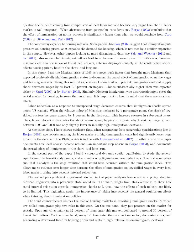
question the evidence coming from comparisons of local labor markets because they argue that the US labormarket is well integrated. When abstracting from geographic considerations, Borjas (2003) concludes thatthe effect of immigration on native workers is significantly larger than what we would conclude from Card(2009) or Ottaviano and Peri (2012).

The controversy expands to housing markets. Some papers, like Saiz (2007) suggest that immigration putspressure on housing prices, as it expands the demand for housing, which is not met by a similar expansionin the supply. However, other papers looking at more disaggregate data, see Saiz and Wachter (2011) andSa (2015), also report that immigrant inflows lead to a decrease in house prices. In both cases, however,it is not clear how the inflow of low-skilled workers, entering disproportionately in the construction sector,affects housing prices, both in the short- and long-run.

In this paper, I use the Mexican crisis of 1995 as a novel push factor that brought more Mexicans thanexpected to historically high-immigration states to document the causal effect of immigration on native wagesand housing markets. Using this natural experiment I show that a 1 percent immigration-induced supplyshock decreases wages by at least 0.7 percent on impact. This is substantially higher than was reportedeither by Card (2009) or by Borjas (2003). Similarly, Mexican immigrants, who disproportionately enter therental market for housing, increase the rental gap. It is important to keep in mind that these are short-runeffects.

Labor relocation as a response to unexpected wage decreases ensures that immigration shocks spreadacross US regions. When the relative inflow of Mexicans increases by 1 percentage point, the share of low-skilled workers increases almost by 1 percent in the first year. This increase reverses in subsequent years.Thus, labor relocation dissipates the shock across space, helping to explain why low-skilled wage growthbetween 1990 and 2000 was only slightly lower in initially high-immigration locations.

At the same time, I have shown evidence that, when abstracting from geographic considerations like inBorjas (2003), age cohorts entering the labor markets in high-immigration years had significantly lower wagegrowth in the decade of the 1990s, which is in line with Oreopoulos et al. (2012). In other words, this paperdocuments how local shocks become national, an important step absent in Borjas (2003), and documentsthe causal effect of immigration in the short- and long- run.

In the second part of the paper I build a structural dynamic spatial equilibrium to study the generalequilibrium, the transition dynamics, and a number of policy-relevant counterfactuals. The first counterfac-tual that I analyze is the wage evolution that would have occurred without the immigration shock. Thisallows me to evaluate over longer-time horizons the effect of immigration on low-skilled wages in every locallabor market, taking into account internal relocation.

The second policy-relevant experiment studied in the paper analyzes how effective a policy stoppingMexican migration into a particular state would be. The main insight from this exercise is to show howrapid internal relocation spreads immigration shocks and, thus, how the effects of such policies are likelyto be limited. This highlights, again, the importance of taking into account the general equilibrium effectswhen thinking about immigration policies.

The third counterfactual studies the role of housing markets in absorbing immigrant shocks. Mexicanlow-skilled immigrants play two roles in this case. On the one hand, they put pressure on the market forrentals. Upon arrival as many as 82 percent of them enter this market, compared to around 30 percent oflow-skilled natives. On the other hand, many of them enter the construction sector, decreasing costs, andgenerating a downward trend in housing prices and rents in high- relative to low-immigrant locations.

37

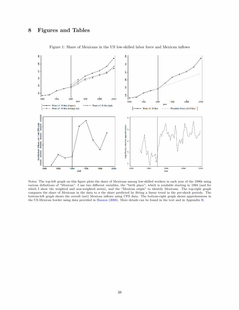
8 Figures and Tables

Figure 1: Share of Mexicans in the US low-skilled labor force and Mexican inflows

Notes: The top-left graph on this figure plots the share of Mexicans among low-skilled workers in each year of the 1990s usingvarious definitions of “Mexican”. I use two different variables, the “birth place”, which is available starting in 1994 (and forwhich I show the weighted and non-weighted series), and the “Mexican origin” to identify Mexicans. The top-right graphcompares the share of Mexicans in the data to a the share predicted by fitting a linear trend in the pre-shock periods. Thebottom-left graph shows the overall (net) Mexican inflows using CPS data. The bottom-right graph shows apprehensions inthe US-Mexican border using data provided in Hanson (2006). More details can be found in the text and in Appendix B.

38

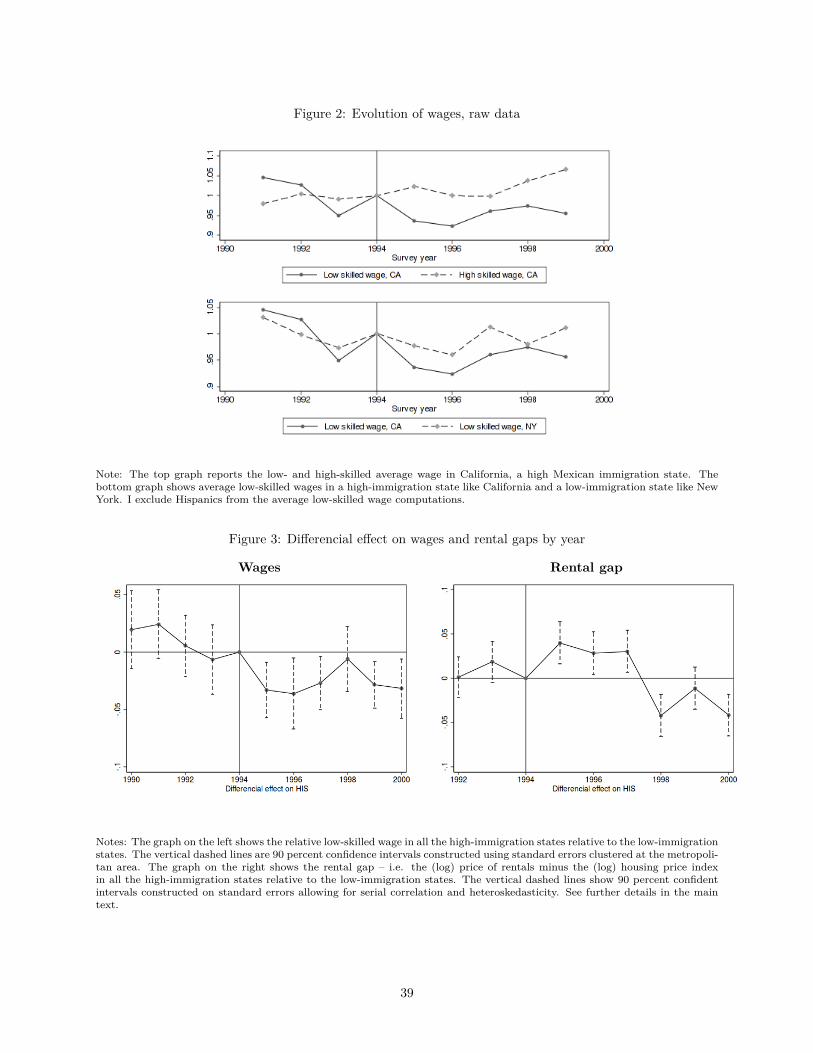
Figure 2: Evolution of wages, raw data

Note: The top graph reports the low- and high-skilled average wage in California, a high Mexican immigration state. Thebottom graph shows average low-skilled wages in a high-immigration state like California and a low-immigration state like NewYork. I exclude Hispanics from the average low-skilled wage computations.

Figure 3: Differencial effect on wages and rental gaps by year

Wages Rental gap

Notes: The graph on the left shows the relative low-skilled wage in all the high-immigration states relative to the low-immigrationstates. The vertical dashed lines are 90 percent confidence intervals constructed using standard errors clustered at the metropoli-tan area. The graph on the right shows the rental gap – i.e. the (log) price of rentals minus the (log) housing price indexin all the high-immigration states relative to the low-immigration states. The vertical dashed lines show 90 percent confidentintervals constructed on standard errors allowing for serial correlation and heteroskedasticity. See further details in the maintext.

39

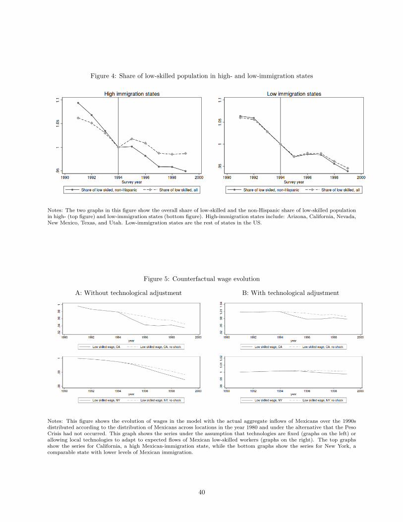
Figure 4: Share of low-skilled population in high- and low-immigration states

Notes: The two graphs in this figure show the overall share of low-skilled and the non-Hispanic share of low-skilled populationin high- (top figure) and low-immigration states (bottom figure). High-immigration states include: Arizona, California, Nevada,New Mexico, Texas, and Utah. Low-immigration states are the rest of states in the US.

Figure 5: Counterfactual wage evolution

A: Without technological adjustment B: With technological adjustment

Notes: This figure shows the evolution of wages in the model with the actual aggregate inflows of Mexicans over the 1990sdistributed according to the distribution of Mexicans across locations in the year 1980 and under the alternative that the PesoCrisis had not occurred. This graph shows the series under the assumption that technologies are fixed (graphs on the left) orallowing local technologies to adapt to expected flows of Mexican low-skilled workers (graphs on the right). The top graphsshow the series for California, a high Mexican-immigration state, while the bottom graphs show the series for New York, acomparable state with lower levels of Mexican immigration.

40

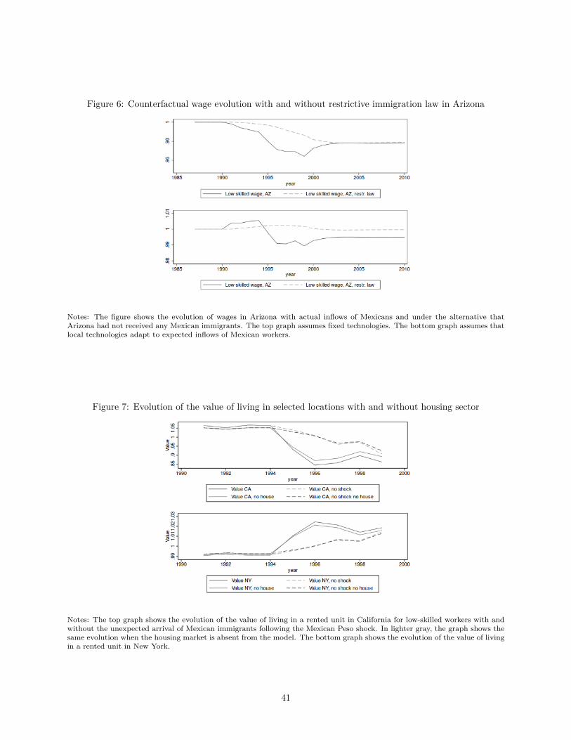
Figure 6: Counterfactual wage evolution with and without restrictive immigration law in Arizona

Notes: The figure shows the evolution of wages in Arizona with actual inflows of Mexicans and under the alternative thatArizona had not received any Mexican immigrants. The top graph assumes fixed technologies. The bottom graph assumes thatlocal technologies adapt to expected inflows of Mexican workers.

Figure 7: Evolution of the value of living in selected locations with and without housing sector

Notes: The top graph shows the evolution of the value of living in a rented unit in California for low-skilled workers with andwithout the unexpected arrival of Mexican immigrants following the Mexican Peso shock. In lighter gray, the graph shows thesame evolution when the housing market is absent from the model. The bottom graph shows the evolution of the value of livingin a rented unit in New York.

41

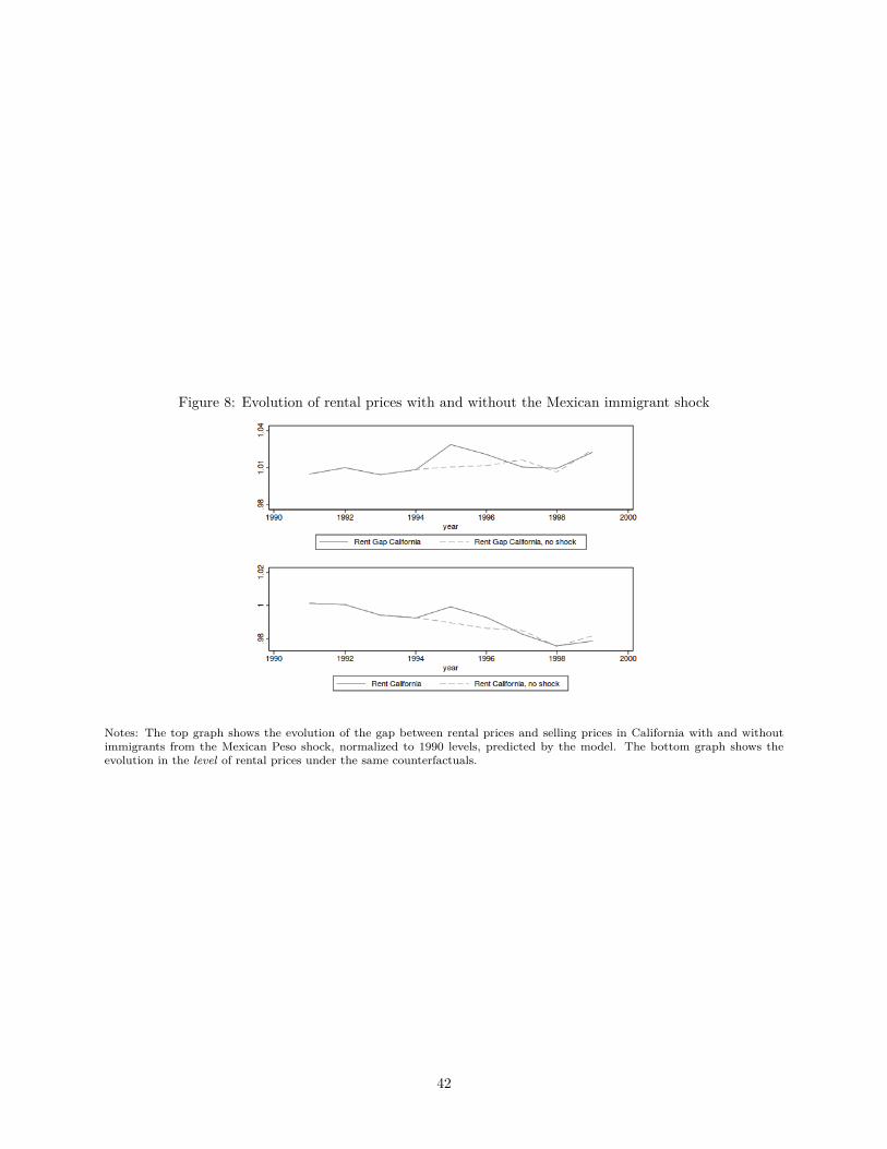
Figure 8: Evolution of rental prices with and without the Mexican immigrant shock

Notes: The top graph shows the evolution of the gap between rental prices and selling prices in California with and withoutimmigrants from the Mexican Peso shock, normalized to 1990 levels, predicted by the model. The bottom graph shows theevolution in the level of rental prices under the same counterfactuals.

42

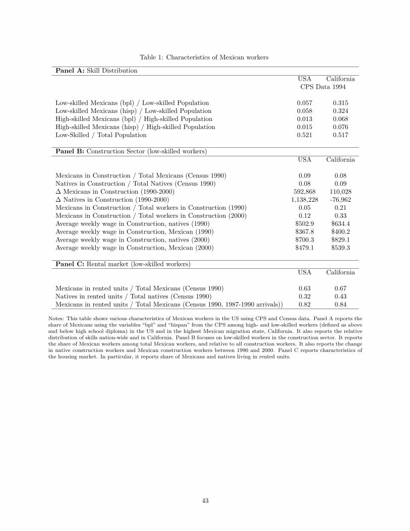
Table 1: Characteristics of Mexican workers

Panel A: Skill DistributionUSA CaliforniaCPS Data 1994

Low-skilled Mexicans (bpl) / Low-skilled Population 0.057 0.315Low-skilled Mexicans (hisp) / Low-skilled Population 0.058 0.324High-skilled Mexicans (bpl) / High-skilled Population 0.013 0.068High-skilled Mexicans (hisp) / High-skilled Population 0.015 0.076Low-Skilled / Total Population 0.521 0.517

Panel B: Construction Sector (low-skilled workers)USA California

Mexicans in Construction / Total Mexicans (Census 1990) 0.09 0.08Natives in Construction / Total Natives (Census 1990) 0.08 0.09∆ Mexicans in Construction (1990-2000) 592,868 110,028∆ Natives in Construction (1990-2000) 1,138,228 -76,962Mexicans in Construction / Total workers in Construction (1990) 0.05 0.21Mexicans in Construction / Total workers in Construction (2000) 0.12 0.33Average weekly wage in Construction, natives (1990) $502.9 $634.4Average weekly wage in Construction, Mexican (1990) $367.8 $400.2Average weekly wage in Construction, natives (2000) $700.3 $829.1Average weekly wage in Construction, Mexican (2000) $479.1 $539.3

Panel C: Rental market (low-skilled workers)USA California

Mexicans in rented units / Total Mexicans (Census 1990) 0.63 0.67Natives in rented units / Total natives (Census 1990) 0.32 0.43Mexicans in rented units / Total Mexicans (Census 1990, 1987-1990 arrivals)) 0.82 0.84

Notes: This table shows various characteristics of Mexican workers in the US using CPS and Census data. Panel A reports theshare of Mexicans using the variables “bpl” and “hispan” from the CPS among high- and low-skilled workers (defined as aboveand below high school diploma) in the US and in the highest Mexican migration state, California. It also reports the relativedistribution of skills nation-wide and in California. Panel B focuses on low-skilled workers in the construction sector. It reportsthe share of Mexican workers among total Mexican workers, and relative to all construction workers. It also reports the changein native construction workers and Mexican construction workers between 1990 and 2000. Panel C reports characteristics ofthe housing market. In particular, it reports share of Mexicans and natives living in rented units.

43

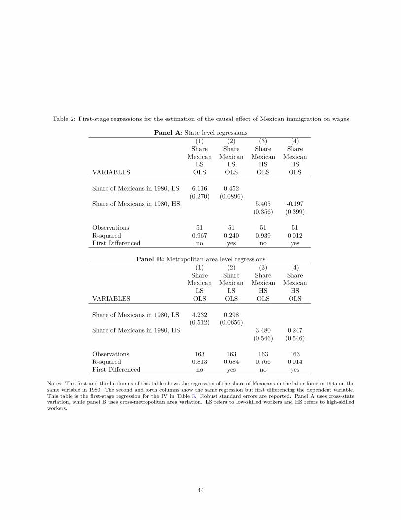
Table 2: First-stage regressions for the estimation of the causal effect of Mexican immigration on wages

Panel A: State level regressions(1) (2) (3) (4)

Share Share Share ShareMexican Mexican Mexican Mexican

LS LS HS HSVARIABLES OLS OLS OLS OLS

Share of Mexicans in 1980, LS 6.116 0.452(0.270) (0.0896)

Share of Mexicans in 1980, HS 5.405 -0.197(0.356) (0.399)

Observations 51 51 51 51R-squared 0.967 0.240 0.939 0.012First Differenced no yes no yes

Panel B: Metropolitan area level regressions(1) (2) (3) (4)

Share Share Share ShareMexican Mexican Mexican Mexican

LS LS HS HSVARIABLES OLS OLS OLS OLS


Share of Mexicans in 1980, HS 3.480 0.247(0.546) (0.546)

Observations 163 163 163 163R-squared 0.813 0.684 0.766 0.014First Differenced no yes no yes

Notes: This first and third columns of this table shows the regression of the share of Mexicans in the labor force in 1995 on thesame variable in 1980. The second and forth columns show the same regression but first differencing the dependent variable.This table is the first-stage regression for the IV in Table 3. Robust standard errors are reported. Panel A uses cross-statevariation, while panel B uses cross-metropolitan area variation. LS refers to low-skilled workers and HS refers to high-skilledworkers.

44

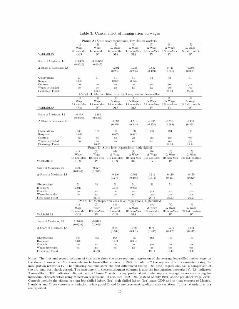
Table 3: Causal effect of immigration on wages

Panel A: State level regressions, low-skilled workers(1) (2) (3) (4) (5) (6) (7)

Wage Wage ∆ Wage ∆ Wage ∆ Wage ∆ Wage ∆ WageLS non-Mex LS non-Mex LS non-Mex LS non-Mex LS non-Mex LS non-Mex LS Ind. controls

VARIABLES OLS IV OLS OLS IV IV IV

Share of Mexicans, LS 0.00499 -0.000791(0.0620) (0.0645)

∆ Share of Mexicans, LS -0.602 -0.733 -0.832 -0.721 -0.708(0.234) (0.265) (0.439) (0.381) (0.307)

Observations 51 51 51 51 51 51 51R-squared 0.000 0.077 0.125Controls no no no yes yes yes yesWages detrended no no no no no yes yesFirst-stage F-stat 511.5 26.73 26.73

Panel B: Metropolitan area level regressions, low-skilled(1) (2) (3) (4) (5) (6) (7)



Share of Mexicans, LS -0.115 -0.186(0.0525) (0.0383)


Observations 163 163 163 163 163 163 163R-squared 0.046 0.055 0.082Controls no no no yes yes yes yesWages detrended no no no no no yes yesFirst-stage F-stat 68.33 19.14 19.14

Panel C: State level regressions, high-skilled(1) (2) (3) (4) (5) (6) (7)

Wage Wage ∆ Wage ∆ Wage ∆ Wage ∆ Wage ∆ WageHS non-Mex HS non-Mex HS non-Mex HS non-Mex HS non-Mex HS non-Mex HS Ind. controls


Share of Mexicans, LS 0.109 0.127(0.0940) (0.0810)

∆ Share of Mexicans, LS -0.246 -0.301 0.114 0.119 0.170(0.273) (0.288) (0.414) (0.441) (0.229)

Observations 51 51 51 51 51 51 51R-squared 0.025 0.013 0.062Controls no no no yes yes yes yesWages detrended no no no no no yes yesFirst-stage F-stat 511.5 26.73 26.73 26.73

Panel D: Metropolitan area level regressions, high-skilled(1) (2) (3) (4) (5) (6) (7)

Wage Wage ∆ Wage ∆ Wage ∆ Wage ∆ Wage ∆ WageHS non-Mex HS non-Mex HS non-Mex HS non-Mex HS non-Mex HS non-Mex HS Ind. controls


Share of Mexicans, LS 0.00828 -0.0165(0.0529) (0.0699)


Observations 163 163 163 163 163 163 163R-squared 0.000 0.011 0.034Controls no no no yes yes yes yesWages detrended no no no no no yes yesFirst-stage F-stat 68.33 19.14 19.14 19.14

Notes: The first and second columns of this table show the cross-sectional regression of the average low-skilled native wage onthe share of low-skilled Mexicans relative to low-skilled workers in 1995. In column 2 the regression is instrumented using theimmigration networks IV. The following columns show the first differenced (using 1994 data) regressions, i.e. a comparison ofthe pre- and post-shock period. The instrument in these subsequent columns is also the immigration networks IV. ‘LS’ indicates‘Low-skilled’. ‘HS’ indicates ‘High-skilled’. Column 7, which is my preferred estimate, reports average wages controlling forindividual characteristics using Mincerian regressions. It also uses 1992-1994 (instead of only 1994) as the pre-shock wage levels.Controls include the change in (log) low-skilled labor, (log) high-skilled labor, (log) state GDP and in (log) exports to Mexico.Panels A and C use cross-state variation, while panel B and D use cross-metropolitan area variation. Robust standard errorsare reported.

45

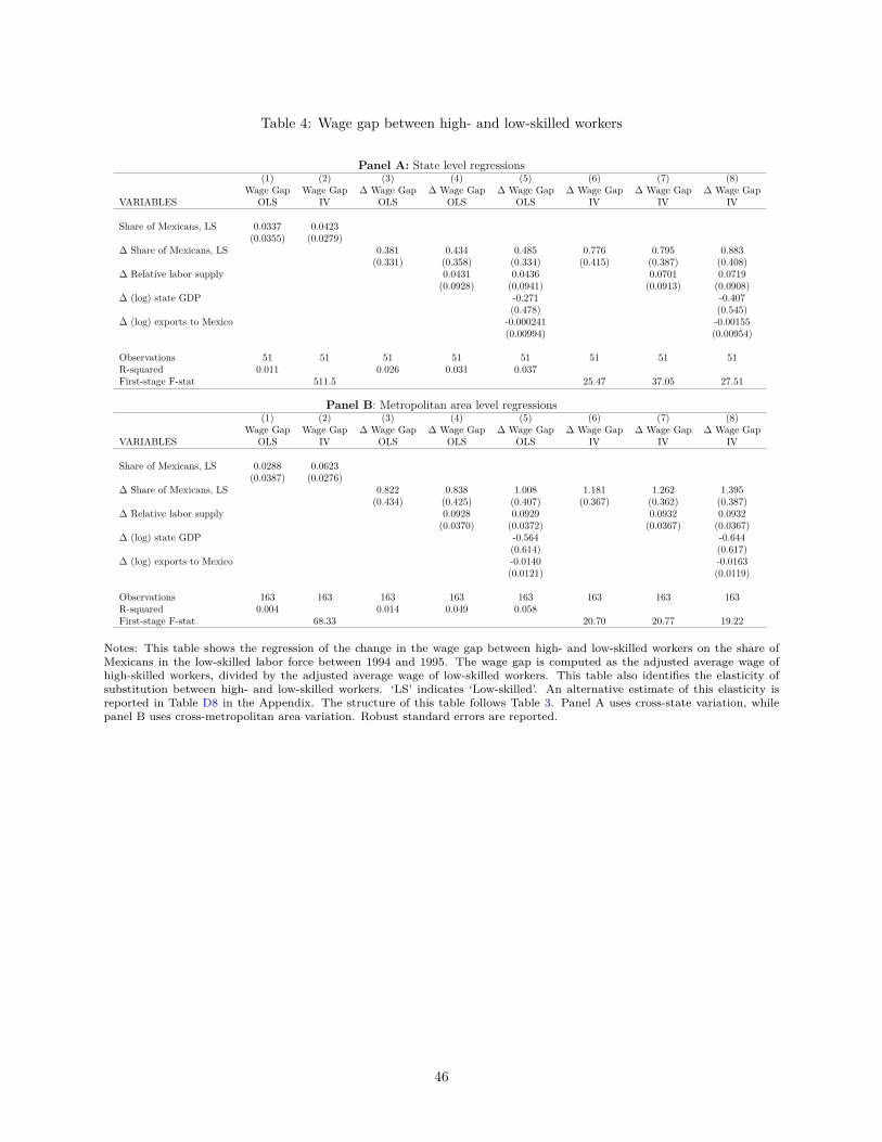
Table 4: Wage gap between high- and low-skilled workers

Panel A: State level regressions(1) (2) (3) (4) (5) (6) (7) (8)

Wage Gap Wage Gap ∆ Wage Gap ∆ Wage Gap ∆ Wage Gap ∆ Wage Gap ∆ Wage Gap ∆ Wage GapVARIABLES OLS IV OLS OLS OLS IV IV IV


∆ Share of Mexicans, LS 0.381 0.434 0.485 0.776 0.795 0.883(0.331) (0.358) (0.334) (0.415) (0.387) (0.408)

∆ Relative labor supply 0.0431 0.0436 0.0701 0.0719(0.0928) (0.0941) (0.0913) (0.0908)

∆ (log) state GDP -0.271 -0.407(0.478) (0.545)

∆ (log) exports to Mexico -0.000241 -0.00155(0.00994) (0.00954)

Observations 51 51 51 51 51 51 51 51R-squared 0.011 0.026 0.031 0.037First-stage F-stat 511.5 25.47 37.05 27.51

Panel B: Metropolitan area level regressions(1) (2) (3) (4) (5) (6) (7) (8)

Wage Gap Wage Gap ∆ Wage Gap ∆ Wage Gap ∆ Wage Gap ∆ Wage Gap ∆ Wage Gap ∆ Wage GapVARIABLES OLS IV OLS OLS OLS IV IV IV


∆ Share of Mexicans, LS 0.822 0.838 1.008 1.181 1.262 1.395(0.434) (0.425) (0.407) (0.367) (0.362) (0.387)

∆ Relative labor supply 0.0928 0.0929 0.0932 0.0932(0.0370) (0.0372) (0.0367) (0.0367)

∆ (log) state GDP -0.564 -0.644(0.614) (0.617)

∆ (log) exports to Mexico -0.0140 -0.0163(0.0121) (0.0119)

Observations 163 163 163 163 163 163 163 163R-squared 0.004 0.014 0.049 0.058First-stage F-stat 68.33 20.70 20.77 19.22

Notes: This table shows the regression of the change in the wage gap between high- and low-skilled workers on the share ofMexicans in the low-skilled labor force between 1994 and 1995. The wage gap is computed as the adjusted average wage ofhigh-skilled workers, divided by the adjusted average wage of low-skilled workers. This table also identifies the elasticity ofsubstitution between high- and low-skilled workers. ‘LS’ indicates ‘Low-skilled’. An alternative estimate of this elasticity isreported in Table D8 in the Appendix. The structure of this table follows Table 3. Panel A uses cross-state variation, whilepanel B uses cross-metropolitan area variation. Robust standard errors are reported.

46

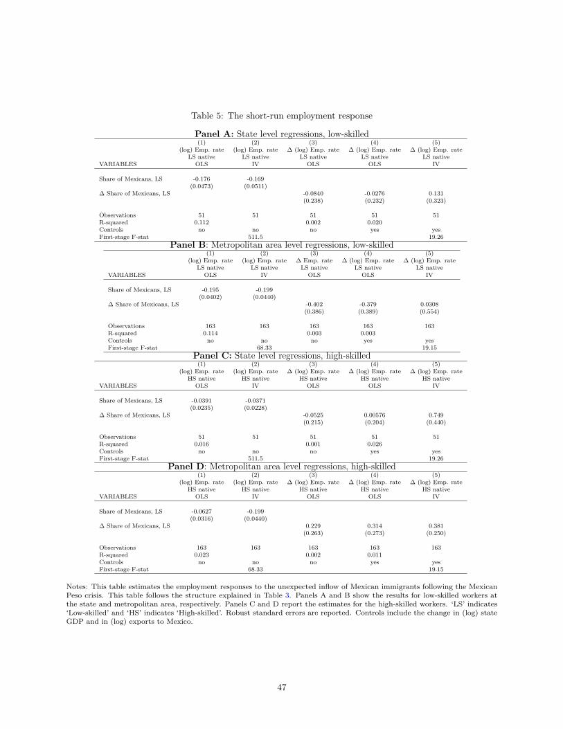
Table 5: The short-run employment response

Panel A: State level regressions, low-skilled(1) (2) (3) (4) (5)

(log) Emp. rate (log) Emp. rate ∆ (log) Emp. rate ∆ (log) Emp. rate ∆ (log) Emp. rateLS native LS native LS native LS native LS native

VARIABLES OLS IV OLS OLS IV


∆ Share of Mexicans, LS -0.0840 -0.0276 0.131(0.238) (0.232) (0.323)

Observations 51 51 51 51 51R-squared 0.112 0.002 0.020Controls no no no yes yesFirst-stage F-stat 511.5 19.26

Panel B: Metropolitan area level regressions, low-skilled(1) (2) (3) (4) (5)

(log) Emp. rate (log) Emp. rate ∆ Emp. rate ∆ (log) Emp. rate ∆ (log) Emp. rateLS native LS native LS native LS native LS native



∆ Share of Mexicans, LS -0.402 -0.379 0.0308(0.386) (0.389) (0.554)


Panel C: State level regressions, high-skilled(1) (2) (3) (4) (5)

(log) Emp. rate (log) Emp. rate ∆ (log) Emp. rate ∆ (log) Emp. rate ∆ (log) Emp. rateHS native HS native HS native HS native HS native



∆ Share of Mexicans, LS -0.0525 0.00576 0.749(0.215) (0.204) (0.440)


Panel D: Metropolitan area level regressions, high-skilled(1) (2) (3) (4) (5)

(log) Emp. rate (log) Emp. rate ∆ (log) Emp. rate ∆ (log) Emp. rate ∆ (log) Emp. rateHS native HS native HS native HS native HS native



∆ Share of Mexicans, LS 0.229 0.314 0.381(0.263) (0.273) (0.250)


Notes: This table estimates the employment responses to the unexpected inflow of Mexican immigrants following the MexicanPeso crisis. This table follows the structure explained in Table 3. Panels A and B show the results for low-skilled workers atthe state and metropolitan area, respectively. Panels C and D report the estimates for the high-skilled workers. ‘LS’ indicates‘Low-skilled’ and ‘HS’ indicates ‘High-skilled’. Robust standard errors are reported. Controls include the change in (log) stateGDP and in (log) exports to Mexico.

47

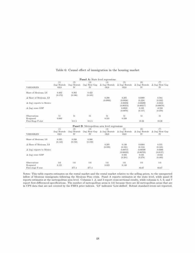
Table 6: Causal effect of immigration in the housing market

Panel A: State level regressions(1) (2) (3) (4) (5) (6) (7)

(log) Rentals (log) Rentals (log) Rent Gap ∆ (log) Rentals ∆ (log) Rentals ∆ (log) Rentals ∆ (log) Rent GapVARIABLES OLS IV IV OLS OLS IV IV

Share of Mexicans, LS 0.402 0.382 0.422(0.172) (0.186) (0.185)

∆ Share of Mexicans, LS 0.298 0.285 0.0388 0.584(0.0993) (0.0938) (0.228) (0.332)

∆ (log) exports to Mexico -0.00356 -0.00298 -0.0344(0.00353) (0.00317) (0.00670)

∆ (log) state GDP 0.0933 0.185 -0.550(0.0970) (0.157) (0.370)

Observations 51 51 51 51 51 51 51R-squared 0.083 0.221 0.239First-Stage F-stat 511.5 511.5 19.26 19.26

Panel B: Metropolitan area level regressions(1) (2) (3) (4) (5) (6) (7)

(log) Rentals (log) Rentals (log) Rent Gap ∆ (log) Rentals ∆ (log) Rentals ∆ (log) Rentals ∆ (log) Rent GapVARIABLES OLS IV IV OLS OLS IV IV

Share of Mexicans, LS 0.335 0.338 0.380(0.143) (0.158) (0.159)

∆ Share of Mexicans, LS 0.205 0.130 0.0304 0.555(0.229) (0.191) (0.153) (0.165)

∆ (log) exports to Mexico -0.00715 -0.00598 -0.0366(0.00833) (0.00795) (0.0127)

∆ (log) state GDP 0.505 0.535 -0.834(0.281) (0.278) (0.403)

Observations 141 141 141 141 141 141 141R-squared 0.121 0.023 0.140First-stage F-stat 377.4 377.4 83.67 83.67

Notes: This table reports estimates on the rental market and the rental market relative to the selling prices, to the unexpectedinflow of Mexican immigrants following the Mexican Peso crisis. Panel A reports estimates at the state level, while panel Breports estimates at the metropolitan area level. Columns 1 ,2, and 3 report cross-sectional results, while columns 4, 5, 6, and 7report first-differenced specifications. The number of metropolitan areas is 141 because there are 22 metropolitan areas that arein CPS data that are not covered by the FHFA price indexes. ‘LS’ indicates ‘Low-skilled’. Robust standard errors are reported.

48

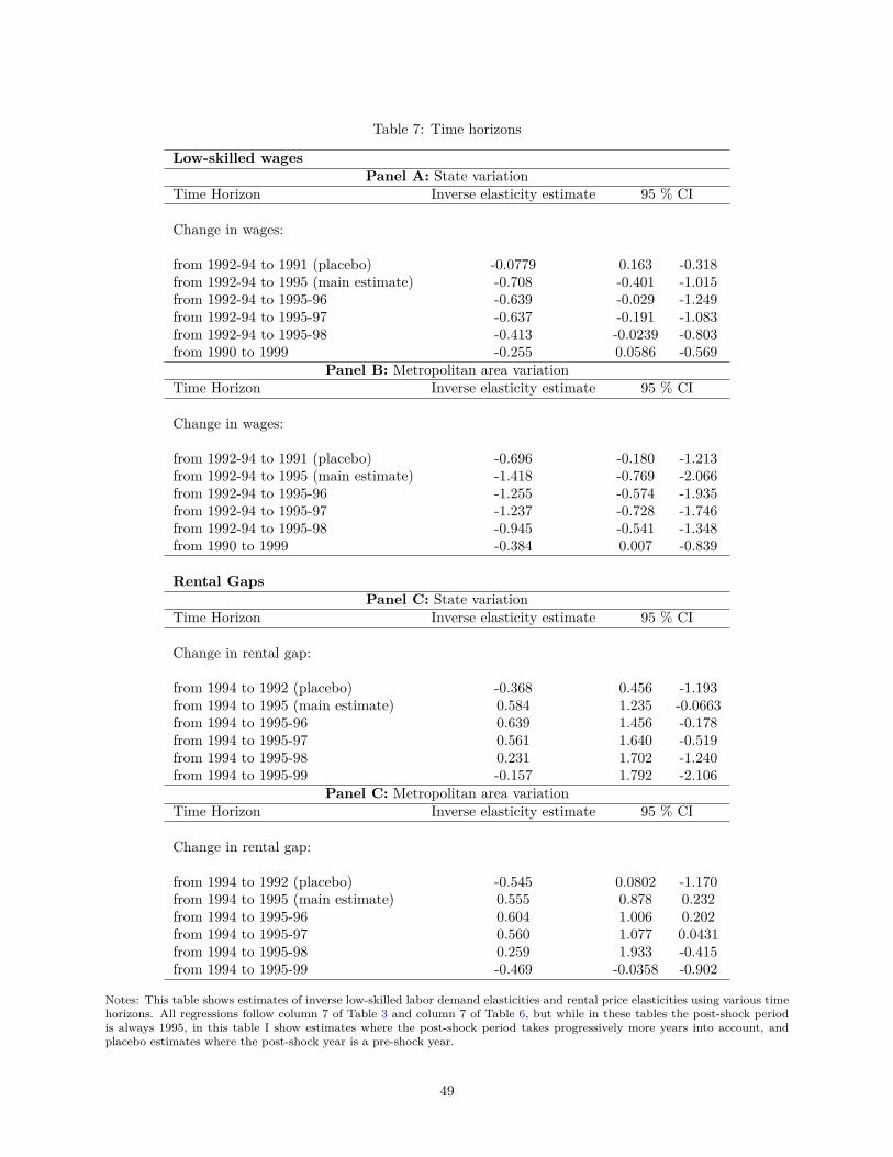
Table 7: Time horizons

Low-skilled wagesPanel A: State variation

Time Horizon Inverse elasticity estimate 95 % CI

Change in wages:

from 1992-94 to 1991 (placebo) -0.0779 0.163 -0.318from 1992-94 to 1995 (main estimate) -0.708 -0.401 -1.015from 1992-94 to 1995-96 -0.639 -0.029 -1.249from 1992-94 to 1995-97 -0.637 -0.191 -1.083from 1992-94 to 1995-98 -0.413 -0.0239 -0.803from 1990 to 1999 -0.255 0.0586 -0.569

Panel B: Metropolitan area variationTime Horizon Inverse elasticity estimate 95 % CI

Change in wages:

from 1992-94 to 1991 (placebo) -0.696 -0.180 -1.213from 1992-94 to 1995 (main estimate) -1.418 -0.769 -2.066from 1992-94 to 1995-96 -1.255 -0.574 -1.935from 1992-94 to 1995-97 -1.237 -0.728 -1.746from 1992-94 to 1995-98 -0.945 -0.541 -1.348from 1990 to 1999 -0.384 0.007 -0.839

Rental GapsPanel C: State variation

Time Horizon Inverse elasticity estimate 95 % CI

Change in rental gap:

from 1994 to 1992 (placebo) -0.368 0.456 -1.193from 1994 to 1995 (main estimate) 0.584 1.235 -0.0663from 1994 to 1995-96 0.639 1.456 -0.178from 1994 to 1995-97 0.561 1.640 -0.519from 1994 to 1995-98 0.231 1.702 -1.240from 1994 to 1995-99 -0.157 1.792 -2.106

Panel C: Metropolitan area variationTime Horizon Inverse elasticity estimate 95 % CI

Change in rental gap:

from 1994 to 1992 (placebo) -0.545 0.0802 -1.170from 1994 to 1995 (main estimate) 0.555 0.878 0.232from 1994 to 1995-96 0.604 1.006 0.202from 1994 to 1995-97 0.560 1.077 0.0431from 1994 to 1995-98 0.259 1.933 -0.415from 1994 to 1995-99 -0.469 -0.0358 -0.902

Notes: This table shows estimates of inverse low-skilled labor demand elasticities and rental price elasticities using various timehorizons. All regressions follow column 7 of Table 3 and column 7 of Table 6, but while in these tables the post-shock periodis always 1995, in this table I show estimates where the post-shock period takes progressively more years into account, andplacebo estimates where the post-shock year is a pre-shock year.

49

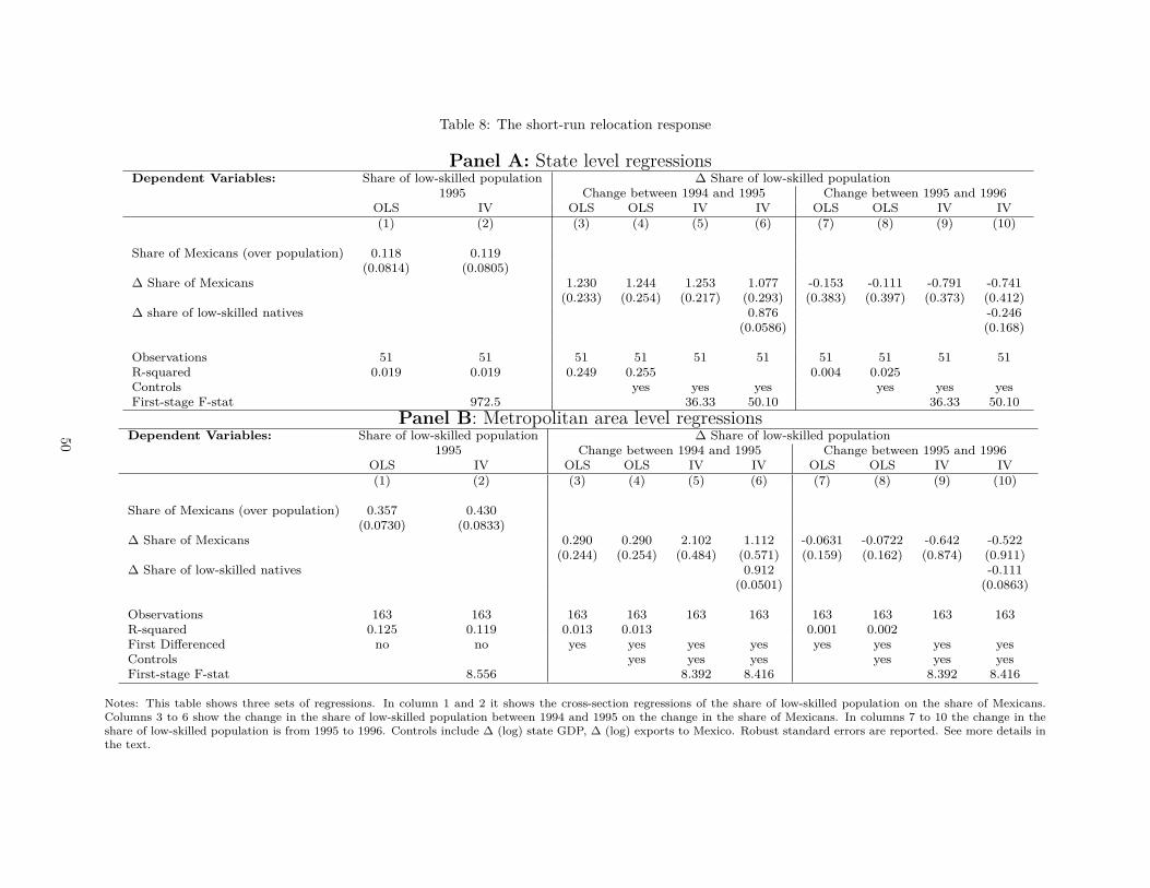
Table 8: The short-run relocation response

Panel A: State level regressionsDependent Variables: Share of low-skilled population ∆ Share of low-skilled population

1995 Change between 1994 and 1995 Change between 1995 and 1996OLS IV OLS OLS IV IV OLS OLS IV IV(1) (2) (3) (4) (5) (6) (7) (8) (9) (10)

Share of Mexicans (over population) 0.118 0.119(0.0814) (0.0805)

∆ Share of Mexicans 1.230 1.244 1.253 1.077 -0.153 -0.111 -0.791 -0.741(0.233) (0.254) (0.217) (0.293) (0.383) (0.397) (0.373) (0.412)

∆ share of low-skilled natives 0.876 -0.246(0.0586) (0.168)

Observations 51 51 51 51 51 51 51 51 51 51R-squared 0.019 0.019 0.249 0.255 0.004 0.025Controls yes yes yes yes yes yesFirst-stage F-stat 972.5 36.33 50.10 36.33 50.10

Panel B: Metropolitan area level regressionsDependent Variables: Share of low-skilled population ∆ Share of low-skilled population

1995 Change between 1994 and 1995 Change between 1995 and 1996OLS IV OLS OLS IV IV OLS OLS IV IV(1) (2) (3) (4) (5) (6) (7) (8) (9) (10)

Share of Mexicans (over population) 0.357 0.430(0.0730) (0.0833)

∆ Share of Mexicans 0.290 0.290 2.102 1.112 -0.0631 -0.0722 -0.642 -0.522(0.244) (0.254) (0.484) (0.571) (0.159) (0.162) (0.874) (0.911)

∆ Share of low-skilled natives 0.912 -0.111(0.0501) (0.0863)

Observations 163 163 163 163 163 163 163 163 163 163R-squared 0.125 0.119 0.013 0.013 0.001 0.002First Differenced no no yes yes yes yes yes yes yes yesControls yes yes yes yes yes yesFirst-stage F-stat 8.556 8.392 8.416 8.392 8.416

Notes: This table shows three sets of regressions. In column 1 and 2 it shows the cross-section regressions of the share of low-skilled population on the share of Mexicans.Columns 3 to 6 show the change in the share of low-skilled population between 1994 and 1995 on the change in the share of Mexicans. In columns 7 to 10 the change in theshare of low-skilled population is from 1995 to 1996. Controls include ∆ (log) state GDP, ∆ (log) exports to Mexico. Robust standard errors are reported. See more details inthe text.

50

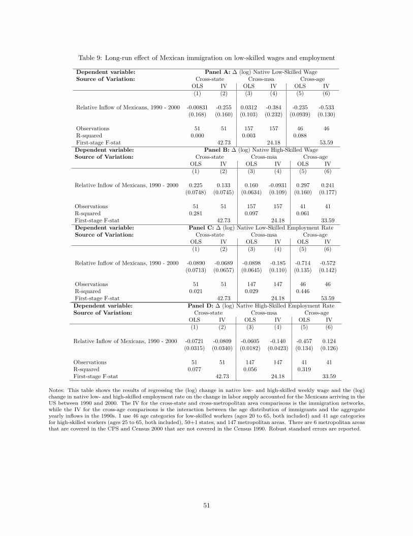
Table 9: Long-run effect of Mexican immigration on low-skilled wages and employment

Dependent variable: Panel A: ∆ (log) Native Low-Skilled WageSource of Variation: Cross-state Cross-msa Cross-age

OLS IV OLS IV OLS IV(1) (2) (3) (4) (5) (6)

Relative Inflow of Mexicans, 1990 - 2000 -0.00831 -0.255 0.0312 -0.384 -0.235 -0.533(0.168) (0.160) (0.103) (0.232) (0.0939) (0.130)

Observations 51 51 157 157 46 46R-squared 0.000 0.003 0.088First-stage F-stat 42.73 24.18 53.59Dependent variable: Panel B: ∆ (log) Native High-Skilled WageSource of Variation: Cross-state Cross-msa Cross-age


Relative Inflow of Mexicans, 1990 - 2000 0.225 0.133 0.160 -0.0931 0.297 0.241(0.0748) (0.0745) (0.0634) (0.109) (0.160) (0.177)

Observations 51 51 157 157 41 41R-squared 0.281 0.097 0.061First-stage F-stat 42.73 24.18 33.59Dependent variable: Panel C: ∆ (log) Native Low-Skilled Employment RateSource of Variation: Cross-state Cross-msa Cross-age


Relative Inflow of Mexicans, 1990 - 2000 -0.0890 -0.0689 -0.0898 -0.185 -0.714 -0.572(0.0713) (0.0657) (0.0645) (0.110) (0.135) (0.142)

Observations 51 51 147 147 46 46R-squared 0.021 0.029 0.446First-stage F-stat 42.73 24.18 53.59Dependent variable: Panel D: ∆ (log) Native High-Skilled Employment RateSource of Variation: Cross-state Cross-msa Cross-age


Relative Inflow of Mexicans, 1990 - 2000 -0.0721 -0.0809 -0.0605 -0.140 -0.457 0.124(0.0315) (0.0340) (0.0182) (0.0423) (0.134) (0.126)

Observations 51 51 147 147 41 41R-squared 0.077 0.056 0.319First-stage F-stat 42.73 24.18 33.59

Notes: This table shows the results of regressing the (log) change in native low- and high-skilled weekly wage and the (log)change in native low- and high-skilled employment rate on the change in labor supply accounted for the Mexicans arriving in theUS between 1990 and 2000. The IV for the cross-state and cross-metropolitan area comparisons is the immigration networks,while the IV for the cross-age comparisons is the interaction between the age distribution of immigrants and the aggregateyearly inflows in the 1990s. I use 46 age categories for low-skilled workers (ages 20 to 65, both included) and 41 age categoriesfor high-skilled workers (ages 25 to 65, both included), 50+1 states, and 147 metropolitan areas. There are 6 metropolitan areasthat are covered in the CPS and Census 2000 that are not covered in the Census 1990. Robust standard errors are reported.

51

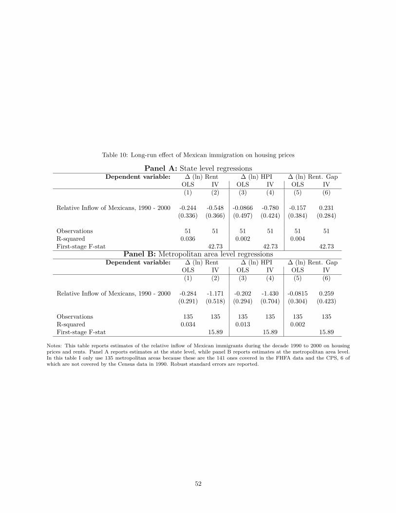
Table 10: Long-run effect of Mexican immigration on housing prices

Panel A: State level regressionsDependent variable: ∆ (ln) Rent ∆ (ln) HPI ∆ (ln) Rent. Gap




Panel B: Metropolitan area level regressionsDependent variable: ∆ (ln) Rent ∆ (ln) HPI ∆ (ln) Rent. Gap




Notes: This table reports estimates of the relative inflow of Mexican immigrants during the decade 1990 to 2000 on housingprices and rents. Panel A reports estimates at the state level, while panel B reports estimates at the metropolitan area level.In this table I only use 135 metropolitan areas because these are the 141 ones covered in the FHFA data and the CPS, 6 ofwhich are not covered by the Census data in 1990. Robust standard errors are reported.

52

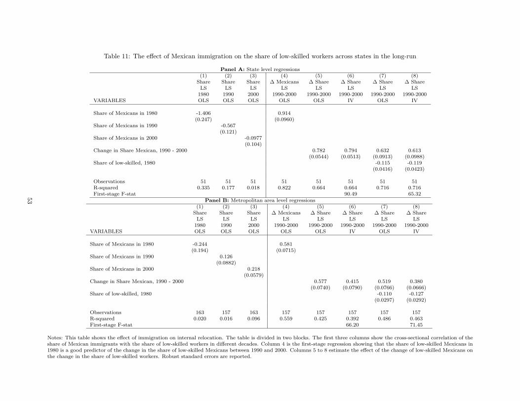
Table 11: The effect of Mexican immigration on the share of low-skilled workers across states in the long-run


Share Share Share ∆ Mexicans ∆ Share ∆ Share ∆ Share ∆ ShareLS LS LS LS LS LS LS LS1980 1990 2000 1990-2000 1990-2000 1990-2000 1990-2000 1990-2000

VARIABLES OLS OLS OLS OLS OLS IV OLS IV

Share of Mexicans in 1980 -1.406 0.914(0.247) (0.0960)

Share of Mexicans in 1990 -0.567(0.121)

Share of Mexicans in 2000 -0.0977(0.104)

Change in Share Mexican, 1990 - 2000 0.782 0.794 0.632 0.613(0.0544) (0.0513) (0.0913) (0.0988)

Share of low-skilled, 1980 -0.115 -0.119(0.0416) (0.0423)

Observations 51 51 51 51 51 51 51 51R-squared 0.335 0.177 0.018 0.822 0.664 0.664 0.716 0.716First-stage F-stat 90.49 65.32


Share Share Share ∆ Mexicans ∆ Share ∆ Share ∆ Share ∆ ShareLS LS LS LS LS LS LS LS1980 1990 2000 1990-2000 1990-2000 1990-2000 1990-2000 1990-2000

VARIABLES OLS OLS OLS OLS OLS IV OLS IV

Share of Mexicans in 1980 -0.244 0.581(0.194) (0.0715)

Share of Mexicans in 1990 0.126(0.0882)

Share of Mexicans in 2000 0.218(0.0579)

Change in Share Mexican, 1990 - 2000 0.577 0.415 0.519 0.380(0.0740) (0.0790) (0.0766) (0.0666)

Share of low-skilled, 1980 -0.110 -0.127(0.0297) (0.0292)

Observations 163 157 163 157 157 157 157 157R-squared 0.020 0.016 0.096 0.559 0.425 0.392 0.486 0.463First-stage F-stat 66.20 71.45

Notes: This table shows the effect of immigration on internal relocation. The table is divided in two blocks. The first three columns show the cross-sectional correlation of theshare of Mexican immigrants with the share of low-skilled workers in different decades. Column 4 is the first-stage regression showing that the share of low-skilled Mexicans in1980 is a good predictor of the change in the share of low-skilled Mexicans between 1990 and 2000. Columns 5 to 8 estimate the effect of the change of low-skilled Mexicans onthe change in the share of low-skilled workers. Robust standard errors are reported.

53

References

Abramitzky, R., L.P. Boustan, and K. Eriksson, “Europe’s Tired, Poor, Huddled Masses: Self-Selection and Economic Outcomes in the Age of Mass Migration,” American Economic Review, 2012.

, , and , “A Nation of Immigrants: Assimilation and Economic Outcomes in the Age of MassMigration,” Journal of Political Economy, 2014.

Acemoglu, D. and D. Autor, “Skills, Tasks and Technologies: Implications for Employment and Earn-ings,” Handbook of Labor Economics Volume 4, Orley Ashenfelter and David E. Card (eds.), 2011.

Adao, R., M. Kolesar, and E. Morales, “Shift-Share Designs: Theory and Inference,” mimeo, 2018.

Ahlfeldt, G., S. Redding, D. Sturm, and N. Wolf, “The Economics of Density: Evidence from theBerlin Wall,” Econometrica, 2015.

Albert, C. and J. Monras, “Immigration and Spatial Equilibrium: the Role of Expenditures in theCountry of Origin,” mimeo, 2019.

Allen, T. and C. Arkolakis, “Trade and the Topography of the Spatial Economy,” Quarterly Journal ofEconomics, 2014.

and D. Donaldson, “Geography and Path Dependence,” mimeo, 2018.

Altonji, J. and D. Card, The Effects of Immigration on the Labor Market Outcomes of Less-Skilled Natives,in John Abowd and Richard Freeman (eds.), Immigration, Trade, and the Labor Market, University ofChicago Press, 1991.

Angrist, J. and A. Kugler, “Protective or Counter-Productive? European Labor Market Institutions andthe Effect of Immigrants on EU Natives,” The Economic Journal, 2003, pp. F302–F331.

and S. Pischke, Mostly Harmless Econometrics: An Empiricist’s Companion, Princeton UniversityPress, 2009.

Autor, D., D. Dorn, and D. Hanson, “The China Syndrome: Local Labor Market Effects of ImportCompetition in the United States,” American Economic Review, 2013, 103(6), 2121–2168.

, , and , “The Geography of Trade and Technology Shocks in the United States,” American EconomicReview Papers and Proceedings, 2013.

Bartik, T. J., “Who Benefits from State and Local Economic Development Policies?,” Books from UpjohnPress. W.E. Upjohn Institute for Employment Research, 1991.

Beaudry, P., E. Lewis, and M. Doms, “Should the PC be Considered a Technological Revolution?Evidence from US Metropolitan Areas,” Journal of Political Economy, 2010, 118(5), 988–1036.

Bertrand, M., E. Duflo, and S. Mullainathan, “How Much Should We Trust Differences-In-DifferencesEstimates?,” Quarterly Journal of Economics, 2004, 119(1), 249–275.

Blanchard, O. and L. Katz, “Regional Evolutions,” Brookings Papers on Economic Activity, 1992, pp. 1–75.

54

Bogin, A., W.M. Doerner, and W.D. Larson, “Local House Price Dynamics: New Indices and StylizedFacts,” FHFA Working Paper 16-01, 2016.

Borjas, G., “The Labor Demand Curve is Downward Sloping: Reexamining the Impact of Immigration onthe Labor Market,” Quarterly Journal of Economics, 2003, pp. 1335–1374.

, “The Wage Impact of the Marielitos: A Reappraisal,” Industrial and Labor Relations Review, 2017.

and J. Monras, “The Labor Market Consequences of Refugee Supply Shocks,” Economic Policy, 2017,32(91), 361–413.

and L. Katz, “The Evolution of the Mexican Born Workforce in the United States,” Mexican Immigrationto the United States, Borjas ed., 2007.

, R. Freeman, and L. Katz, “How Much Do Immigration and Trade Affect Labor Market Outcomes?,”Brookings Papers on Economic Activity, 1997, pp. 1–67.

Borusyak, K., P. Hull, and X Jaravel, “Quasi-experimental Shift-share Designs,” mimeo, 2018.

Boustan, L.P., “Was Postwar Suburbanization ’White Flight’? Evidence from the Black Migration,”Quarterly Journal of Economics, 2010.

Caballero, E., B. Cadena, and B. Kovak, “Measuring Geographic Migration Patterns Using MatrÃculasConsulares,” Demography, 2018.

Caliendo, L., F. Parro, E. Rossi-Hansberg, and P-D. Sartre, “The Impact of Regional and SectoralProductivity Changes on the U.S. Economy,” Review of Economic Studies, Forthcoming.

, M. Dvorkin, and F. Parro, “Trade and Labor Market Dynamics,” NBER Working Paper No. 21149,2015.

Calvo, G. and E. Mendoza, “Petty Crime and Cruel Punishment: Lessons from the Mexican Debacle,”American Economic Review Papers and Proceedings, 1996, 86(2), 170–175.

Card, D., “The Impact of the Mariel Boatlift on the Miami Labor Market,” Industrial and Labor RelationsReview, 1990, pp. 245–257.

, “Immigrant Inflows, Native Outflows and the Local Labor Market Impacts of Higher Immigration,”Journal of Labor Economics, 2001, 19.

, “Is The New Immigration Really So Bad?,” Economic Journal, 2005, 115, 300–323.

, “Immigration and Inequality,” American Economic Review Papers and Proceedings, 2009, 99(2), 1–21.

, A. Mas, and J. Rothstein, “Tipping and the Dynamics of Segregation,” Quarterly Journal of Eco-nomics, 2008, 123(1).

and E. Lewis, “The Diffusion of Mexican Immigrants During the 1990s: Explanations and Impacts,”Mexican Immigration to the United States, 2007, George J. Borjas (ed), University of Chicago Press.

and J. DiNardo, “Do immigrant Inflows lead to Native Outflows,” American Economic Review, 2000.

55

Clemens, M. and J. Hunt, “The Labor Market Effects of Refugee Waves: Reconciling Conflicting Results,”Industrial and Labor Relations Review, 2018.

, E. Lewis, and H. Postel, “Immigration Restrictions as Active Labor Market Policy: Evidence fromthe Mexican Bracero Exclusion,” American Economic Review, 2018, 108(6), 1468–87.

Cohen-Goldner, S. and D. Paserman, “The dynamic impact of immigration on natives’ labor marketoutcomes: Evidence from Israel,” European Economic Review, 2011.

Combes, P-P. and L. Gobillon, “The Empirics of Agglomeration Economics,” Handbook of Regional andUrban Economics, 2014.

Davis, M. and F. Ortalo-Magne, “Household Expenditures, Wages, Rents,” Review of Economic Dy-namics, 2011.

Diamond, R., “The Determinants and Welfare Implications of US Workers’ Diverging Location Choices bySkill: 1980-2000,” American Economic Review, 2015.

Dustmann, C., T. Frattini, and I. Preston, “The Effect of Immigration along the Distribution ofWages,” Review of Economic Studies, 2013.

, U. Schonberg, and J. Stuhler, “Labor Supply Shocks and the Dynamics of Local Wages and Em-ployment,” Quarterly Journal of Economics, 2017.

Foged, M. and G. Peri, “Immigrants and Native Workers: New Analysis Using Longitudinal Employer-Employee Data,” American Economic Journal: Applied Economics, 2016, 8(2), 1–34.

Friedberg, R., “The Impact of Mass Migration on the Israeli Labor Market,” Quarterly Journal of Eco-nomics, 2001, pp. 1373–1408.

Glaeser, E., Cities, Agglomeration and Spatial Equilibrium, Oxford University Press, 2008.

Glitz, A., “The Labor Market Impact of Immigration: A Quasi-Experiment Exploiting Immigrant LocationRules in Germany,” Journal of Labor Economics, 2012, 30(1), 175–213.

Goldsmith-Pinkham, P., I. Sorkin, and H. Swift, “Bartik Instruments: What, When, Why, and How,”NBER WP, 2018.

Gyourko, J. and A. Saiz, “Construction Costs and the Supply o Housing Structure,” Journal of RegionalScience, 2006, 46(4), 661–680.

Hanson, G., “Illegal Migration from Mexico to the United States,” Journal of Economic Literature, 2006,44(4), 869–924.

and A. Spilimbergo, “Illegal Migration, Border Enforcement and Relatvie Wages: Evidence fromApprehensions at US-Mexico Border,” American Economic Review, 1999, 89(5), 1337–1357.

Hanushek, E. and J. Quigley, “What is the price elasticity of housing demand?,” Review of Economicsand Statistics, 1980.

Hornbeck, R., “The Enduring Impact of the American Dust Bowl: Short- and Long-run Adjustments toEnvironmental Catastrophe,” American Economic Review, 2012, 102(4), 1477–1507.

56

and S. Naidu, “When the Levee Breaks: Black Migration and Economic Development in the AmericanSouth,” NBER WP n. 18296, 2012.

Hunt, J., “The Impact of the 1962 Repatriates from Algeria on the French Labor Market,” Industrial andLabor Relations Review, 1992.

Imbert, C. and J. Papp, “Short-term Migration, Rural Public Works and Urban Labor Markets: Evidencefrom India,” Journal of the European Economic Association, Forthcoming.

Jaeger, D., J. Ruist, and J. Stuhler, “Shift-share Instruments and the Impact of Immigration,” NBERworking paper, 2018.

Katz, L and K. Murphy, “Changes in Relative Wages, 1963-1987: Supply and Demand Factors,” QuarterlyJournal of Economics, 1992, 107(1), 35–78.

Kennan, J. and J. Walker, “The Effect of Expected Income on Individual Migration Decisions,” Econo-metrica, 2011, 79(1), 211–251.

Lewis, E., “Immigration, Skill Mix, and Capital-Skill Complementarity,” Quarterly Journal of Economics,2012, 126(1), 1029–1069.

Llull, J., “The Effect of Immigration on Wages: Exploiting Exogenous Variation at the National Level,”Journal of Human Resources, 2017, Forthcoming.

MacKinnon, J. and M. Webb, “Wild Bootstrap Inference for Wildly Different Cluster Sizes,” Journalof Applied Econometrics, 2016.

Martin, J., “Can We Control the Border? A Look at Recent Efforts in San Diego, El Paso and Nogales,”Center for Immigration Studies, 1995.

Mayo, S.K., “Theory and estimation in the economics of housing demand,” Journal of Urban Economics,1981.

Monras, J., “Economic Shocks and Internal Migration,” IZA Discussion Paper No. 8840, 2015.

, “Immigration and Wage Dynamics: Evidence from the Mexican Peso Crisis,” IZA Discussion Paper No.8924, 2015.

, “Economic Shocks and Internal Migration,” CEPR Discusion Paper 12977, 2018.

, “Immigration, Internal Migration, and Technology Adoption,” mimeo, 2019.

Monte, F., F. Redding, and E. Rossi-Hansberg, “Commuting, Migration and Local EmploymentElasticities,” American Economic Review, Forthcoming.

Moretti, E., “Local Labor Markets,” Handbook of Labor Economics, 2011.

Morten, M. and G. Bryan, “The Aggregate Productivity Effects of Internal Migration: Evidence fromIndonesia,” Journal of Political Economy, Forthcoming.

Munshi, K., “Networks in the Modern Economy: Mexican Migrants in the U.S. Labor Market,” QuarterlyJournal of Economics, 2003.

57

Nagy, D., “City location and economic development,” mimeo, 2018.

Nekoei, A., “Immigrants’ Labor Supply and Exchange Rate Volatility,” American Economic Journal:Applied Economics, 2013, 5 (4), 144–164.

Notowidigdo, M., “The Incidence of Local Labor Demand Shocks,” mimeo, 2013.

Oreopoulos, P., T. von Wachter, and A. Heisz, “Short- and Long-Term Career Effects of Graduatingin a Recession,” American Economic Journal: Applied Economics, 2012.

Ottaviano, G. and G. Peri, “Rethinking the Effect of Immigration on Wages,” Journal of the EuropeanEconomic Association, 2012, 10 (1), 152–197.

Passel, J., “Estimates of the Size and Characteristics of the Undocumented Population,” Pew HispanicCenter Report, 2005.

, D. Cohn, and A. Gonzalez-Barrera, “Net Migration from Mexico Falls to Zero and Perhaps Less,”Pew Hispanic Center Report, 2012.

Peri, G. and C. Sparber, “Assessing Inherent Model Bias: An Application to Native Displacement inResponse to Immigration,” Journal of Urban Economics, 2011, 69(1), 82–91.

and V. Yasenov, “The Labor Market Effects of a Refugee Wave: Applying the Synthetic ControlMethod to the Mariel Boatlift,” Journal of Human Resources, 2019, 54(2), 267 – 309.

Quigley, J. and L.A. Rosenthal, “The effects of land use regulation on the price of housing: What dowe know? What can we learn?,” Cityscape, 2005.

Redding, S. and E. Rossi-Hansberg, “Quantitative Spatial Economics,” Annual Review of Economics,2018, 9, 21–58.

Roback, J., “Wages, Rents, and the Quality of Life,” Journal of Political Economy, 1982, 90(6), 1257–1278.

Rosen, S., “Hedonic Prices and Implicit Markets: Product Differentiation in Pure Competition,” Journalof Political Economy, 1974, 82, 34–55.

Ruggles, S., M. Sobek, T. Alexander, C.A. Fitch, R. Goeken, PK Hall, M. King, and C. Ron-nander, “Integrated Public Use Microdata Series: Version 4.0 [Machine-readable database].,”Minneapolis,MN: Minnesota Population Center [producer and distributor], 2016.

Sa, F., “Immigration and housing prices in the UK,” Economic Journal, 2015, 125, 1393–1424.

Saiz, A., “Room in the Kitchen for the Melting Pot: Immigration and Rental Prices,” Review of Economicsand Statistics, 2003, 85(3), 502–521.

, “Immigration and housing rents in American cities,” Journal of Urban Economics, 2007, 61(2), 345–371.

, “The Geographic Determinants of Housing Supply,” Quartely Journal of Economics, 2010, 125(3), 1253–1296.

and S. Wachter, “Immigration and the Neighborhood,” American Economic Journal: Economic Policy,2011, 3(2), 169–188.

58

Topel, R., “Local Labor Markets,” Journal of Political Economy, 1986, 94(3), S111–S143.

Watson, M., “Enforcement and Immigrant Location Choice,” NBER n. 19626, 2013.

Wozniak, A. and T. Murray, “Timing is Everything: Short-run Population Impacts of Immigration inU.S. Cities,” Journal of Urban Economics, 2012, 72(1), 60–78.

59

Everything that follows is for online publication only

The Appendix is organized as follows. In section A I discuss various empirical results that complementthose displayed in the main text. In section B I discuss various details about the data used. In section C Iprovide the proofs of the various propositions in the paper and discuss various generalizations to the modelpresented in the main text. All the figures and tables discussed in this Appendix are shown in section D.

A Appendix: Empirics

A.1 Characteristics of Mexican immigrants

Both in the short-run and long-run estimation I rely on the fact that the characteristics of Mexicans arrivingin different years do not change substantially. While I cannot show that this is indeed the case for unob-servable characteristics, I show in this section that this seems a good approximation for the most relevantcharacteristics.

[Table D3 should be here]

In Table D3 I compare observable characteristics of Mexicans in 1994, in 1995 and 1996. Most variablesare not distinguishable from 0 and for those that are different from 0 the differences are quantitatively verysmall.57

In Figure D.2 I show in more detail the most important observable characteristic both for my long-run identification strategy and for wage determination: age. The figure shows that the age distribution ofMexican arrivals is very similar across years during the 1990s. The total flow of Mexicans is higher in 1995than in other years, despite that all these data is based on the Census 2000 question on the year of arrival,and thus, it capture the high numbers of arrivals occurring close to the Census question, but the distribution,shown in the bottom graph, is almost identical.

[Figure D.2 should be here]

A.2 Discussion on the threads to identification of short-run effects

The main threat to my identification strategy is that the devaluation of the Peso might have changed thetrading relations between US and Mexico. This can have effects on the labor market, as Autor et al. (2013a)show for the case of import competition from China. However, US imports from Mexico did not increase,relative to the trend, as shown in Figure D.3 in the Appendix. This figure also shows that exports from theUS to Mexico in fact saw a significant decrease. If states exporting to Mexico are the same states whereMexican immigrants entered, then I might be confounding the effect of trade and immigration. Fortunately,even if there is some overlap, immigrants do not systematically enter states that export heavily to Mexico.The unconditional correlation between the relative immigration flows and the share of exports to Mexico

57This suggests that over short-time horizons selection does not play an important role. This is different than what mayhappen over (much) longer time horizons as explored in Abramitzky et al. (2012) and Abramitzky et al. (2014) using historicaldata during the Age of Mass migration.

60

(relative to state GDP) is below .5. Similarly, in an OLS regression with state and time fixed effects thecovariance between these two variables is indistinguishable from 0.58


Furthermore, even if exports to Mexico and immigration from Mexico occurred in the same states, itis harder to explain through trade why the effects of immigration are concentrated only on workers withsimilar characteristics to the Mexican inflows. I document the largest labor market impacts on low-skilledworkers in high-immigration states and no effects on high-skilled workers, which matches the nature of theimmigration shock.

To avoid the possible contamination of my estimates from the direct effect of trade on wages I include insome of my regressions (log) US states’ exports to Mexico and (log) state GDP. This should control for thepossible direct effect of trade on the US labor market.59

Another thread to identification is that maybe the characteristics of Mexicans who arrived in 1995 aredifferent than Mexicans arriving in other years. As mentioned in section 2.1 and discussed in more detailin the Appendix section A.1, Figure D.2 and Table D3, this does not seem to be the case. The observablecharacteristics of the Mexican immigrants in the US do not change significantly before and after 1995.Assuming that labor-market relevant unobservable characteristics like ability are correlated with observablecharacteristics, changing Mexican immigrant characteristics before and after 1995 does not seem to be animportant thread for my identification strategy.

A third thread to my identification strategy is that perhaps the real exchange rate changed the incentivesto send remittances back to Mexico, affecting local economies. This is hard to control for since its importanceis proportional to the relative size of the Mexican work force at the local level. There are at least two waysin which changes in the exchange rate could affect local labor markets. On the one hand, it could bethat Mexicans in the US decided to send more or less remittances as a function of the appreciation of thedollar. This could lead to decreases or increases in local consumption that could affect the labor market. Tothe extend that changes in local consumption affect both high- and low-skilled intensive products in localeconomies equally this does not pose a thread to my identification strategy. Another option is related tothe work by Nekoei (2013). He provides evidence that a depreciation of the foreing currencies lead to adecrease in earnings and hours worked of immigrant workers in the US. He explains this finding through theeffect that the real exchange rate has on remittances. However, an alternative reading of his evidence is thatperhaps earnings decrease precisely because more migrants move to the US, particularly when exchange ratefluctuations lead to profound economic crisis as was the case in 1995. In any case, not controlling for theeffect that remittances may have on intensive margin labor supply decisions as explored in Nekoei (2013),tends to make my estimates smaller, and thus not controlling for it is a conservative strategy. Decreases inhours worked would imply decreases in the labor supply of Mexicans already in the US and would, in part,attenuate the wage impact of new inflows.

58 In the case of California, the state receiving the largest amount of immigrants, the ratio of US exports to Mexico relative tostate GDP was below .7 percent throughout the decade. Other states, like Texas, Michigan, Arizona, Alabama, Louisiana, SouthCarolina, and Delaware, have higher or very similar ratios of exports to Mexico to GDP. In other words, Mexican immigrationis substantially more important for California than exports to Mexico.

59Data for state exports to Mexico is provided by WISERTrade (www.wisertrade.org), based on the US Census Bureau.Exports are computed using “state of origin”. “state of origin” is not defined as the state of manufacture, but rather as thestate where the product began its journey to the port of export. It can also be the state of consolidation of shipments. Thoughimperfect, this is the best data available, to my knowledge, on international exports from US states.

61

Finally, it is worth mentioning that the networks instrument that I use could be improved if I hadinformation on the exact place of origin of the immigrants within Mexico. As Munshi (2003) shows, thereare tight links between particular parts of Mexico and particular destinations in the US. In this context, Icould potentially use the intensity of the crisis across Mexican locations to better predict the intensity ofthe flows into the US. Unfortunately, data of this sort, representative at the Mexican national level is onlyavailable starting at around 2006, see Caballero et al. (2018).

A.3 Geography robustness

An important robustness check is to see whether the short-run results on wages are driven by California orTexas exclusively. I do so by excluding these two states, from the OLS and IV regressions presented in Table3.


Table D5 shows very similar estimates independent of whether I drop California or Texas. The first-stageusing state level variation is a little weak when dropping Texas, something that does not occur when usingmetropolitan area variation. Figure D.4 provides visual evidence of the strength of the first-stage whendropping California or Texas.


A.4 Substitutability between high school dropouts and graduates

A second important robustness check is to use only high school dropouts or high school graduates whencomputing low-skilled wages. Borjas (2003) distinguishes these two groups suggesting that they are imperfectsubstitutes, while Card (2009) strongly criticizes this assumption.


Table D6 shows that the results are similar between high school dropouts and high school graduates.This is consistent with Card (2009) argument that these two types of workers are closely competing. Thestandard errors increase for the smaller group of high school dropouts, as should be the case.

A.5 Excluding foreign-born from the computation of non-Mexicans wages

A final robustness check that I present is that instead of excluding only Mexicans from the computation oflow-skilled wages, I exclude all non-US foreign-born. Doing so does not change the results, as can be seenin Table D7


62

A.6 Alternative methods to compute the inverse demand elasticity

In the main text I use the following regression to obtain the elasticity of substitution between high- andlow-skilled workers:

∆ ln hsws

= α+ β1 ∗∆MexsNs

+ ∆Xs ∗ γ + εs (20)

This equation can be obtained from realizing that the relative labor demand can be written as:

ln( hw

) = α− 1σ

ln( LH

)

And that, α − 1σ ln( LH )) = α − 1

σ ln(Mexicans+non-Mexican low-skilled) + 1σ ln(H) = α − 1

σ ln(1 +(Mexicans/Non-Mexican low-skilled))− 1

σ ln(Non-Mexican low-skilled)+ 1σ ln(H) ≈ α− 1

σ ( MexicansNon-Mexican low-skilled )−

1σ ln(Non-Mexican low-skilled) + 1

σ ln(H) = α− 1σ ( Mexicans

Non-Mexican low-skilled ) + 1σ ln(Non-Mexican low-skilled/H).

Taking first differences from this equation we obtain the estimating equation 1. If we have exogenous varia-tion for ∆ Mexs

Ns then β exactly recover 1/σ.Note that an alternative method is to directly use:

∆ ln( hsws

) = α+ β2∆ ln( LsHS

) + εs (21)

In order to use this equation to estimate β2 we need exogenous variation in the change of the (log) skillratio ∆ ln( LH ).

We can use the inflow of Mexican workers to obtain such variation. If Mexican workers entered randomlyacross locations then we could use as a first-stage the following equation 22 (where I distinguish N and L asN should not include Mexicans):

∆ ln(LsHs

) = α+ δ1∆MexsNs

+ ∆Xs ∗ γ + εs (22)

With this first-stage we can then estimate the elasticity of substitution between L and H. As argued inthe main text, though, Mexican workers don’t necessarily enter local markets randomly. For this, we canfurther instrument equation 22 with the networks instrument. Thus, in order to estimate 1/σ we would needa three step procedure. A three step procedure is numerically equivalent to using the networks instrumentto directly instrument the change in the log skill ratio. This is:

∆ ln(LsHs

) = α+ δ2 ∗Mex1980

s

N1980s

+ ∆Xs ∗ γ + εs (23)

To show that any of the two methods delivers very similar estimates, i.e. that β1 ≈ β2 I report in TableD8 all of these regressions.


In column 1, I show that the initial share of Mexicans in 1980 weakly predicts the change in the (log) skillratio between 1994 and 1995. Many Mexicans moved to high-immigration locations, but at the same timenatives are an important part of the change in the skill ratio, thus introducing some noise into the regression.This noise doesn’t bias the estimate (which is very similar to the first-stage shown in Table 2), but it doesdecrease precision. Column 2, explicitly shows that the increase in the skill ratio is entirely driven by Mexican

63

migration between 1994 and 1995. Both using across-state and across metropolitan area variation I obtainan estimate very close to 1. Column 3 uses the networks instrument to account for the endogenous locationchoice of Mexicans. The IV estimate is also close to 1. Column 4 shows the reduced form estimate of theIV on the wage gap. It shows that places with initially high shares of Mexicans experienced an increase inthe wage gap between 1994 and 1995. Column 5, is the OLS regression of equation 21. It shows that theOLS estimate is equal to 0. It is only when I instrument it with the networks instrument, which lead to anexogenous decrease in the ratio of skilled to low-skilled workers, that I obtain an estimate of around 1. Thisestimate is very similar to the estimate reported in the main text, in Table 4, and reproduced in column 7for convenience. The main difference between columns 6 and 7, is that estimates in column 6 are less precisedue to the fact that the first-stage relation is less strong for the skill ratio than for the share of Mexicans, asone would expect.

A.7 Internal migration

There are various internal and international migration responses that could explain these internal migrationpatterns. For example, it could be that Mexican workers returned to Mexico in 1996, after one year ofthe shock. This is unlikely, given the net inflows observed in the aggregate. Second, it could be that thenon-Mexican workers responded to the shock, either by migrating away from or not migrating into high-immigration states. This is also unlikely. When moving from columns 5 to 6 and from 9 to 10 the onlydifference is that in columns 6 and 10 I include the change in the share of native low-skilled workers. Addingthis control does not change the estimates significantly, suggesting that native low-skilled population did notendogenously respond to the shock. Finally, it could be that the Mexicans first migrated to high-immigrationstates and then further moved within the US. This is likely to be the case, as I show in Figure D.5. Thisfigure looks at the distribution of Mexicans and native low-skilled workers across space over two time periods:1990-1995 and 1995-2000. To describe the evolution in the distribution of people across space I first rankthe states from 1 to 51 by the share of Mexicans (over total Mexicans in the US) in 1990. I then plot the(smoothed) change between the different years. I also do this for the distribution of low-skilled natives.The figure shows some very interesting patterns. As is also documented in Card and Lewis (2007), overthe 90s Mexicans started to spread throughout the US. This is visible in 1990-1995 but it accentuates in1995-2000. More concretely, what this figure shows is that the distribution of Mexicans effectively movedfrom the highest Mexican immigration states (California and Texas) to the states where there were someMexicans but not too many (Arizona and New Mexico).

A.8 Comparing the evidence from the Mexican Peso crisis and the MarielBoatlift

I argue in the main text that my results are consistent with much of the literature. The one study for whichthis appears not to be true is Card’s (1990) landmark study of the Mariel Boatlift. Card (1990) also looked atshort-term effects of immigration inflows but, unlike this paper, found essentially no effects. What explainsthis difference? This section examines it in more detail and I provide additional evidence in Monras (2019).

In April 1980, Fidel Castro allowed Cubans willing to emigrate, to do so from the port of Mariel. TheseCubans – the “Marielitos” – were relatively low-skilled and some of them had allegedly been released fromprisons and mental hospitals by Cuban authorities (Card, 1990). As a result, around 125,000 Cubansmigrated to the US between late April 1980 and October 1980. Around half of them probably settled in

64

Miami. Card (1990) uses this natural experiment to assess the effect of immigration on the labor market.Using a group of four comparison cities – Tampa, Houston, Atlanta, and Los Angeles – Card (1990) reportsno effect of Cuban immigrants on any group of the Miami labor force.60 These findings are contrary to whatis reported in this paper.

An important departure from Card (1990) landmark study is Borjas (2017). He shows that when con-centrating on the group of workers in Miami that are most likely competing with Cuban immigrants – i.e.male high-school drop-outs –, wages in Miami declined after the Mariel Boatlift relative to a number ofcontrol group cities. The magnitude of this decline, given the size of the shock, is similar to the estimates Iprovide in this paper using the Mexican Peso Crisis as exogenous push factor. In both episodes, however, itis important to distinguish between different types of native workers, as some may be positively or negativelyaffected by immigration as a function of education/skill types, see also the discussion in Borjas and Monras(2017).

A difference between Borjas (2017) estimates and my estimates of the effect of Mexican immigrants, isthat the decline in wages in Miami is most pronounced 3 to 5 years after the shock, perhaps reflecting,as Card (1990) suggests, the nature of the “Marielitos” – who were perhaps not ready to enter the labormarket immediately – and/or the particularities of Miami’s labor market. It is worth emphasizing though,that apart from this small delay in the wage effects seen in Miami, the results reported in this paper arevery much in line with the results reported in Borjas (2017) and the internal migration response during theMariel Boatlift episode was also similar as explained in Monras (2019).

The wage effects estimated in Borjas (2017) have been criticized by two papers: Peri and Yasenov (2019)and Clemens and Hunt (2018). These criticisms largely reflect the difficulties that arise when using the MarielBoatlift episode. First, the number of individual level observations in Miami that can be used to computewage trends is small, usually below 30 individuals when restricting the sample to particular education groups.Hence, small changes in how to compute these wage trends may result in large changes in the estimatedaverage wage in Miami. Second, only 38 metropolitan areas are covered by the CPS data in the early 1980sand so the the number of treated and potential control cities is also small. Hence, small changes on how toconstruct adequate control groups may also result in significant changes in the estimate of the wage impact ofimmigration. In contrast, Mexican immigrants are more wide spread within the US, and hence, the variationthat I use in this paper comes from many and not just one treated location and is robust to dropping variouslocations as shown in Table D5 in this Appendix.

My conclusion when comparing the various studies that use variation from the Mariel Boatlift episodeand the estimates using the Mexican Peso crisis is that, as explained here and in more detail in Monras(2019), the evidence coming from these two episodes is not in contradiction to each other.

A.9 Mexican Migration and the Construction Sector

Mexican workers entered disproportionately to the construction sector over the 1990s. As reported in Table 1the share of low-skilled workers working in construction was similar among Mexicans and natives, at around9 percent. Over the 1990s, however, almost 600,000 Mexicans entered the construction sector, which isroughly one third of the total change in construction labor force.

To investigate this more formally I run the following regression:60Card distinguishes by racial groups and quartiles in the wage distribution, but not by education.

65

∆Share Mexicans in Constructions = α+ β ∗ ∆00−90MexsNs,90

+ εa

A coefficient of 1 in this regression would mean that for every Mexican arrival 1 extra Mexican enteredthe construction sector over the 1990s. The results of this regression are striking. As can be seen in TableD10, the estimate fluctuates between .6 and .5 depending on whether I use an OLS specification or an IVspecification, see columns 1 and 2.

Table D10 should be around here

The large entries of Mexican workers could have expanded the relative size of the construction sector, orcould have instead displaced native workers in the sector. To investigate this I run the following regression:

∆Share in Constructions = α+ β ∗ ∆00−90MexsNs,90

+ εa

A coefficient of 0 in this regression means that the construction sector did not grew more in high-immigration locations than in low-immigrant locations. Results are shown in columns 3 and 4 of Table D10.Both with the OLS and especially with the IV specification I obtain a tightly estimated 0.

The final question is whether the fact that so many Mexicans entered the construction sector meant thataverage native wages of low-skilled workers in the sector declined. For that I run the exact same specificationas the long-run wage results shown in section 4.2 but restricting wages to the construction sector. The resultsare also reported in Table D10. It is clear that wages in that sector declined much more than in the overalleconomy. Both using across-state and across-metropolitan area variation the table shows that wages declinedby around .7 to .8 percent for a 1 percent immigration-induced supply shock. This long-run decrease is, inmagnitude, similar to the short-run estimates.

A.10 Housing prices

To think about how Mexican migration may affect housing prices I proceed in two steps. First, I tryto understand whether the cost reduction justifies the observed decrease in housing prices. Second, I tryto recover the price elasticity of the local demand for housing from the decreased prices and increasedconstruction. I then compare my estimates to those in the existing literature.

According to Gyourko and Saiz (2006) the construction sector can be characterized by a perfectly compet-itive model. This is so because, the paper reports that an exogenous increase in construction permits leadsto a very small increase in construction costs and at the same time, it provides summary statistics showingthat the number of firms in the sector is large, and employers mostly have small shares of total employment.Moreover the elasticity of the number of construction establishments to population is very close to one acrosslocations. This leads Gyourko and Saiz (2006) to conclude that: “Such a flat supply schedule suggests acompetitive market with free entry and a large number of price-taking suppliers that produce at minimumaverage cost in the long term. [...] In sum, the stylized facts on the industrial organization of this sectorare quite consistent with constant cost production” (page 672). Second, Gyourko and Saiz (2006) show thatunionization rates are very strong predictor of construction cost differences across metropolitan areas (page673). According to them, this is a consequence of both higher wages and higher than optimal usage of laborin high unionization rate metropolitan areas. Third, Gyourko and Saiz (2006) argue that independently ofunionization rates, differences in wages is the other strong predictor of construction costs differences across

66

metropolitan areas. They argue that this is due to the opportunity cost of labor when choosing to workin construction. Their estimates seem to indicate that the labor share in total costs is at least 60 percent.Finally, among the geographic variables, high hills seem to be the most important, but explains a smallerpart of the data than unionization rates and wage rates.

This means that Mexican immigrants reduces construction costs because they may affect wages, andbecause they may be paid lower wages, perhaps because they are less unionized or for other reasons. Giventhese considerations, we can do the following back of the envelope computations. In a perfect competitivemodel of the housing market we have that:

p = c(w, r) = ( w

1− α )1−α( rα

)α

i.e., prices should be equal to the unit cost. In this case I assume that construction requires capital andlow-skilled labor. We are interested in how an immigrant shock may affect this pricing equation:

∂ ln p∂πmex

= (1− α) ∂ lnw∂πmex

+ α∂ ln r∂πmex

Where πmex denotes the share of Mexican immigrants.61 If capital is elastically supplied as assumedthourghout in the paper and as implied by Gyourko and Saiz (2006) results, then:

∂ ln p∂πmex

= (1− α) ∂ lnw∂πmex

Where πmex denotes the share of Mexican immigrants. Now, average wages are a weighted averagebetween native wages and Mexican wages:

w = (1− πmex)wnat + πmexwmex

When Mexican arrive they change wages because of two reasons. First, they may impact natives wages,I reported causal estimate of ∂ lnwnat

∂πmex ≈ −1.62 Second, they increase the number of Mexican workers whichtypically have lower wages. We can compute these two effects as follows:

∂w

∂πmex= −wnat − (1− πmex)wnat + wmex + πmexwmex

∂ lnwmex

∂πmex

Assuming natives and immigrants are perfect substitutes (i.e. ∂ lnwmex∂πmex = ∂ lnwnat

∂πmex = −1) we can simplifythis further:63

∂w

∂πmex= −wnat − (1− πmex)wnat + wmex − πmexwmex

So, we have that:

∂w

∂πmex= −w − wnat + wmex

61I derive here the results with respect to a change in πmex instead of Mex/N which is what I used in the main text becausefor this exercise the algebra is cleaner this way.

62I could use here the long-run estimate on wages in the construction sector shown in Table D10. This would make ∂ lnwnat∂πmex

≈−.8. Showing the algebra with ∂ lnwnat

∂πmex= −1 makes the exercise much simpler and cleaner. Quantitatively the difference is

not large.63Note that if they were imperfect substitutes then there would be an extra decline coming from the additional effect of

Mexicans on previous Mexicans’ wages. Note also that even if two groups of workers are perfect substitutes, wage levels maybe different. What is crucial is that they move in parallel.

67

which can be re-written as:

∂ lnw∂πmex

= −1− (wnat − wmex)w

This equation illustrates that Mexican migration affects average wages through two channels: the directeffect on wages and the composition effect.

With this, we can return to housing prices and express them as follows:

∂ ln p∂πmex

= −(1− α)(1 + (wnat − wmex)w

)

This equation says that the change in housing prices should be the share of labor in production (at least.6 according to Gyourko and Saiz (2006)) times one plus the difference in wages of natives and Mexicans.This difference in Census data for 1990 and 2000 is around 40 percent.64 Hence, these back of the envelopcomputations suggest that prices should decrease by around .6*1.4=.84. This number is a bit higher thanthe long-run regressions at the state level suggest and a bit lower than what I obtain in the metropolitanarea regressions (although wage effects are also estimated to be larger when using metropolitan area levelvariation). In both cases, however, .84 is well inside the range given by the confidence intervals.

A cost reduction should lead to an expansion in the supply of housing. How much the supply of housingexpands depends on the price elasticity of housing demand. Which we can try to recover using data onnew construction. To investigate this I use data from the “Building Permits Survey”, maintained by the USCensus Bureau. These data contain the number of new residential units by state (as far as I can tell thesedata are not available at the metropolitan area level). With these data I did two exercises. First, I compareCalifornia and NY as I do in most of the paper. Second, I take all the states and I relate new constructionwith the Mexican flows of the 1990s. These data is not available at the metropolitan area level.

Figure D.6 should be around here

In the figure we see that there seems to be more construction in a high Mexican immigration state likeCalifornia than in New York, which is a high migration state but with relatively few Mexican immigrants.The gap seems to widen in around 1996 or 1997. To try to compute the elasticity of new constructionto Mexican inflows over the 1990s I use equation 4. I show the results in table D11, below. I obtain anestimate of this elasticity of around 2. The elasticity of housing prices to Mexican inflows was estimated tobe around -1. This means that I obtain the following elasticity: when new housing construction increases by10 percent, housing prices decline by around 5 percent. I could not find in the literature a direct estimatethat is comparable to this elasticity.

Table D11 should be around here

However, a way to think about the magnitude of my estimates is to realize that new construction repre-sents at least 14 percent of total sales. This is so according to data from the St Louis Fed for 2018. I couldnot find a data series on existing home sales for the 1990s, only quotes or aggregate graphs in websites suchas https://tradingeconomics.com/united-states/existing-home-sales. The National Association of Realtorshave these data, but at a cost. There is data on new home sales from the US Department of Housing and

64Mexican wages are around 32 percent lower than natives. Hence the difference divided by the average wage is around 40 inhigh immigrant locations.

68

Urban Development, shown for example in the St Louis Fed: https://fred.stlouisfed.org/series/HSN1F. Bylooking at these figures I obtain a range of the share of new to total units sold that should comfortably liebetween 15 to 20 percent. If this is correct, it means that an increase in new construction of 10 percentmeans that total units increase by 1.5 to 2 percent, given a decline in house prices of 5 percent. Hence, Iobtain results that are in line with a housing demand elasticity ∂ lnQ

∂ lnP of around -0.3 to -0.4.There is a small and often times not very recent literature that provides comparable estimates. For

example, Hanushek and Quigley (1980) estimate that the price elasticity of housing demand is -0.65 inPittsburgh and -0.45 in Phoenix (see page 451). Mayo (1981) reviews this literature and provides estimatesthat cluster around -0.5 although some estimates are below -.2 and some above -0.8 (in absolute terms).This older literature makes me think that the estimates that I obtain are reasonable.

There is a much larger literature that estimates the effect of regulations on housing prices. It is hardto translate these estimates into an estimate of the price elasticity of the demand for housing, but all ofthis literature finds that increased regulation leads to house price increases. See for example the review ofthe literature in Quigley and Rosenthal (2005). Part of this literature has interpreted the regulations asmaking the supply of housing more inelastic, although some might have shifted the supply of housing, henceproviding implicit estimates of the price elasticity of housing demand.

B Appendix: Data

B.1 Indirect measures of Mexican inflows

In this subsection I look at more indirect measures of Mexican inflows, something that should complementthe direct measures shown in Section 2.1. A first such measure is the marked increase in “coyote” pricesstarting in 1995 – the price of the smuggler who facilitates migration across the Mexican-US border, seeHanson (2006). This may be in part due to increased border enforcement, but it also probably reflects anincreased willingness to emigrate from Mexico. In fact, the US border enforcement launched two operationsin the early 1990s to try to curb the number of immigrants entering the US. Operation Hold the Line andOperation Gatekeeper – launched in El Paso, TX, and San Diego, CA respectively – had different degreesof success (Martin, 1995). Operation Hold the Line managed to curb Mexican immigrants, while OperationGatekeeper was less successful65. To some extent, however, these operations redirected the routes Mexicanstook to get to the US. There is some evidence suggesting that some of the Mexicans who would have otherwiseentered through El Paso, TX did so through Nogales, AZ. In any case, the “coyote” prices only started toincrease in 1995 and not when these operations were launched, suggesting that more people wanted to enterthe US in 1995, right when the Peso Crisis hit Mexico, and that the increased “coyote” prices were not justa result of the increased border enforcement of the early 1990s.

Finally, it is also reassuring that other data sources, like the number of legal Mexican migrants recorded bythe Department of Homeland Security or the number of migrants computed using Immigration NaturalizationService data (Hanson, 2006) also see a spike right after the Peso Crisis.

65Figure D.4 in the Appendix shows that indeed inflows to Texas during the 1990s are more distorted from the initialdistribution than inflows towards California.

69

B.2 Geographic disaggregation

The geographic units that I use in this paper are US states and metropolitan areas. There is some discussionin the literature as to what the appropriate geographic disaggregation to represent a local labor marketis. As explained in the main text, commuting zones and states cover the entire US. However, only urbancommuting zones can be identified in the CPS data throughout the period, since they mostly coincide withthe variable ‘metarea’ – there are a few rural commuting zones that are identified by this variable that I alsouse.

There are 163 metropolitan areas with observations during the 1990s to do the exercise using CPS data.There are 6 of these metropolitan areas, however, that are not covered in the Census of the year 1990. Theseare: Columbus, GA/FL, Fort Walton Beach, FL, Huntsville, AL, Portland, ME, Tallahassee, FL, Topeka,KS. Thus, the long-run regressions only use 157 metropolitan areas.

There are some metropolitan areas for which the FHFA price index and the FMR rental rates are notavailable. This decreases the number of metropolitan areas available when using housing market data from163 to 141. The ones not covered in the housing data are: Ann Arbor, MI, Bridgeport, CT, El Paso, TX, FortLauderdale-Hollywood-Pompano Beach, FL, Fort Walton Beach, FL, Galveston-Texas City, TX, Hamilton-Middleton, OH, Honolulu, HI, Jacksonville, FL, Manchester, NH, New Bedford, MA, Philadelphia, PA/NJ,Santa Barbara-Santa Maria-Lompoc, CA, Sarasota, FL, Seattle-Everett, WA, Stamford, CT, Tacoma, WA,Ventura-Oxnard-Simi Valley, CA, Washington, DC/MD/VA, Waterbury, CT, West Palm Beach-Boca Raton-Delray Beach, FL, Wilmington, DE/NJ/MD, Worcester, MA.

B.3 Definition of Mexicans

When using Census data or post-1994 CPS data I define Mexicans by the place of birth. When using CPSdata before 1994 I use the variable HISPAN from the CPS. I use the category “Mexican(Mexicano)” – value108 – when plotting or using data before 1994. When plotting various years, I keep the definition fixed atthe pre-1994 definition.

For data after 1994 and US Census data, I use the variable BPLD from the March CPS and Census 1990and 2000 files, Ruggles et al. (2016).

B.4 Definition of low-skilled

Low-skilled workers are defined as having a high school diploma or less. I use the variable EDUC from theCPS to do so.

B.5 Definition of worker

I use full-time workers to compute wages. This is constructed using the EMPSTAT variable from the CPS.I exclude from the wage computations workers who are self-employed or in group quarters. I correct for topcoding following the literature. I limit the analysis to workers aged 20 to 65.

B.6 Individual characteristics and weights

In some micro-level Mincerian regressions, I include individual characteristics as controls. These include ageand age square, race dummies (using directly the CPS variable), marital status, and occupation dummies. I

70

aggregate the occupation OCC1990 variable to 24 larger groups, based on the definition of this variable inIpums.

In all the wage computations, regressions, and graphs I use the weights coming from the WTSUPP.For the internal relocation results I do not use weights, and instead focus on individual observations. Thedistribution of weights between natives and immigrants changes dramatically between 1995 and 1996, as canbe seen very clearly in Figure D.7 and Table D3. This could contaminate some of the results on relocation, orin general any regression that compares pre- and post- 1995 data (1994 to 1995 comparisons are fine). Whilethe results using the weights are similar to the ones reported in the paper, using WTSUPP results in moreimprecise estimates. The only significant difference is that when using WTSUPP, there is a net-outflow ofMexicans in 1996. This is unlikely and entirely driven by the change in the distribution of weights between1995 and 1996. For the graphs showing the aggregate Mexican stock and Mexican inflow data I use theaverage weight of all Mexican observations throughout the decade for every year. This gives me a betterestimate of the level of these variables. For the differences (which are used in the regressions) this hardlymatters.


When aggregating to the state level, I use the number of observations used to compute the averages ineach cell. I use this in the regressions, using the analytic weights command from stata.

B.7 Aggregation of occupations

I create these categories following the aggregation proposed in Ruggles et al. (2016): Management Occu-pations, Business Operations Specialists, Financial Specialists, Computer and Mathematical Occupations,Architecture and Engineering Occupations, Life, Physical, and Social Science Occupations, Community andSocial Services Occupations, Legal Occupations, Education, Training, and Library Occupations, Arts, De-sign, Entertainment, Sports, and Media Occupations, Healthcare Practitioners and Technical Occupations,Healthcare Support Occupations, Protective Service Occupations, Food Preparation and Serving Occupa-tions, Building and Grounds Cleaning and Maintenance Occupations, Personal Care and Service Occupa-tions, Sales Occupations, Office and Administrative Support Occupations, Farming, Fishing, and ForestryOccupations, Construction Trades, Extraction Workers, Installation, Maintenance, and Repair Workers,Production Occupations, Transportation and Material Moving Occupations.

C Appendix: Theory

C.1 Direct Utility Formulation

The utility of a household that lives in s and considers living in s′(r) is defined as:

lnU it,s,s′(r) = −ln(α)(1− α) + lnAs′(r) + (1− α) ln ct,s′ + α ln houset,s′(r) + βEt lnUt+1,s′ + εit,s′(r)

The budget constraint, which does not allow for savings, is given by:

ct,s′(r) + pt,s′(r)houset,s′(r) ≤ wt,s′

71

where houset,s′(r) is the amount of squared meters of a unit of housing or the quality of the housing.The maximization of this problem results in:

ct,s′(r) = (1− α)wt,s′

and

houset,s′(r) = αwt,s′

pt,s′(r)

Thus, the indirect utility is given by

lnV it,s,s′(r) = lnVt,s′(r) + εit,s′(r) = lnAs′(r) + lnwt,s′ − α ln pt,s′(r) + βEt lnVt+1,s′ + εit,s′(r)

C.2 Proof of Proposition 1

In this section I prove Proposition 1.To prove this proposition I first use the fact that:

Ns = N−1s + Is −Os

i.e., the population in a location at a given point in time can be decomposed between the populationalready there (N−1

s ), the in-migrants (Is) – people not residing in s that move into s –, and the out-migrants(Os) – people who were living in s that leave.

We can use this expression to see how much population react to a given change in wages:

∂Ns∂ lnws

= ∂N−1s

∂ lnws+ ∂Is∂ lnws

− ∂Os∂ lnws

This can be re-written as follows, using the fact that ∂Ns∂ lnws = Ns

∂ lnNs∂ lnws and that the population in the

previous period cannot react to contemporaneous wage changes that were un-anticipated:

∂lnNs∂ lnws

= IsNs

∂ ln Is∂ lnws

− OsNs

∂ lnOs∂ lnws

Given this expression, I will separately compute the response of the in- and the out-migration rate towage changes. Given the assumptions of the model, ∂ lnOs

∂ lnws ≈ 0. This is so, because a constant fraction ofthe population moves every period, and this constant fraction η does not depend on local conditions. ∂ lnOs

∂ lnwsis not exactly 0 because among the fraction 1− η that decides to relocate, there is a small fraction that maydecide as destination the origin from which it started. If there is a large number of potential destinations,this is, though, a very small fraction. I use this reasoning again below.

To compute ∂ ln Is∂ lnws it is useful to use the definition:

Is =∑j 6=s

Πj,s

where Πj,s is the flow of people moving from origin j to destination s. From this:

∂ ln Is∂ lnws

=∂ ln

∑j 6=s Πj,s

∂ lnws= 1∑

j 6=s Πj,s

∑j 6=s

∂Πj,s

∂ lnws= 1∑

j 6=s Πj,s

∑j 6=s

Πj,s∂ ln Πj,s

∂ lnws

72

Thus, we need to compute ∂ ln Πj,s∂ lnws for j 6= s. For this, we start from the fact that:

Πj,s = ηN−1s

V1/λs′∑j V

1/λj

which follows from equation 10 using the two potential housing markets and where I specify that N−1s is

the population at the start of the period. From this:

ln Πj,s = ln η + lnN−1s + 1

λlnVs′ −

1λ

lnV

where remember that V = (∑j V

1/λj )λ. From this expression:

∂ ln Πj,s

∂ lnws= 0 + 0 + 1

λ

∂ lnVs∂ lnws

− 1λ

∂ lnV∂ lnws

From this expression we need to use the fact that lnVs = 1γ ln

∑r V

1/γs(r) , and that ∂ lnV

∂ lnws is approximately0 when the number of possible destinations is large. Thus:

∂ lnVs∂ lnws

= γ

(∑r V

1/γs(r) )γ

(∑r

V1/γs(r) )γ−1

∑r

∂V1/γs(r)

∂ lnws= 1∑

r V1/γs(r)

∑r

V1/γs(r)

∂ lnVs(r)∂ lnws

From this, we need to find ∂ lnVs(r)∂ lnws . The definition of Vs(r) is:

lnVs(r) = lnAs(r) + lnws − α ln ps(r) + β(1− η) lnV ′s + βη lnV ′

So, from this we obtain

∂ lnVs(r)∂ lnws

≈ 1 + β(1− η)∂ lnV ′s∂ lnws

where again I use the fact that ∂ lnV ′s∂ lnws is approximately 0 when the number of destinations is large.

This expression says that the effect of wages on the value of living in the location is equal to one, plus thediscounted effect on the value of living in that location in the following period. In the long-run equilibriumthis is an iterative process, so that:

∂ lnVs(r)∂ lnws

≈ 1 + β(1− η) + (β(1− η))2 + .. = 11− β(1− η)

Collecting terms, we obtain that:

∂ ln Πj,s

∂ lnws≈ 1λ

∂ lnVs∂ lnws

= 1λ

11− β(1− η)

And so:

∂ ln Is∂ lnws

≈ 1λ

11− β(1− η)

And thus:

∂ lnNs∂ lnws

≈ 1λ

11− β(1− η)

IsNs

73

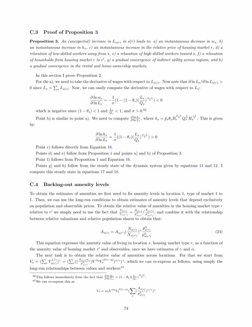
C.3 Proof of Proposition 3

Proposition 3. An (unexpected) increase in Ls(r) in s(r) leads to: a) an instantaneous decrease in ws, b)an instantaneous increase in hs, c) an instantaneous increase in the relative price of housing market r, d) arelocation of low-skilled workers away from s, e) a relocation of high-skilled workers toward s, f) a relocationof households from housing market r to r′, g) a gradual convergence of indirect utility across regions, and h)a gradual convergence in the rental and home-ownership markets.

In this section I prove Proposition 2.For the a), we need to take the derivative of wages with respect to Ls(r). Now note that ∂ lnLs/∂ lnLs(r) >

0 since Ls =∑r Ls(r). Now, we can easily compute the derivative of wages with respect to Ls:

∂ lnws∂ lnLs

= − 1σ

(1− (1− θs)(LsQs

)σ−1σ ) < 0

which is negative since (1− θs) < 1 and LsQs

< 1, and σ > 0.66

Point b) is similar to point a). We need to compute ∂ lnhs∂ lnLs , where hs = p̃sθsB

σ−1σ

s Q1σs H

−1σs . This is given

by:

∂ ln hs∂ lnLs

= 1σ

((1− θs)(LsQs

)σ−1σ ) > 0

Point c) follows directly from Equation 16.Points d) and e) follow from Proposition 1 and points a) and b) of Proposition 3.Point f) follows from Proposition 1 and Equation 16.Points g) and h) follow from the steady state of the dynamic system given by equations 11 and 12. I

compute this steady state in equations 17 and 18.

C.4 Backing-out amenity levels

To obtain the estimates of amenities we first need to fix amenity levels in location 1, type of market 1 to1. Then, we can use the long-run conditions to obtain estimates of amenity levels that depend exclusivelyon population and observable prices. To obtain the relative value of amenities in the housing market type rrelative to r′ we simply need to use the fact that Vs(r)

Vs(r′)= As(r)

pαs(r)

/As(r′)pαs(r′)

, and combine it with the relationshipbetween relative valuations and relative population shares to obtain that:

As(r) = As(r′)(Ns(r)

Ns(r′))γpαs(r)

pαs(r′)(24)

This equation expresses the amenity value of living in location s, housing market type r, as a function ofthe amenity value of housing market r′ and observables, once we have estimates of γ and α.

The next task is to obtain the relative value of amenities across locations. For that we start fromVs = (

∑r V

1/γs(r) )γ = (

∑r((

As(r)wspαs(r)

)V βηV β(1−η)s )1/γ)γ , which we can re-express as follows, using simply the

long-run relationships between values and workers:67

66This follows immediately from the fact that ∂ lnQs∂ lnLs

= (1 − θs)( LsQs )σ−1σ .

67We can re-express this as

Vs = wsVβηV

β(1−η)s (

∑r

(As(r)

pαs(r)

)1/γ)γ

74

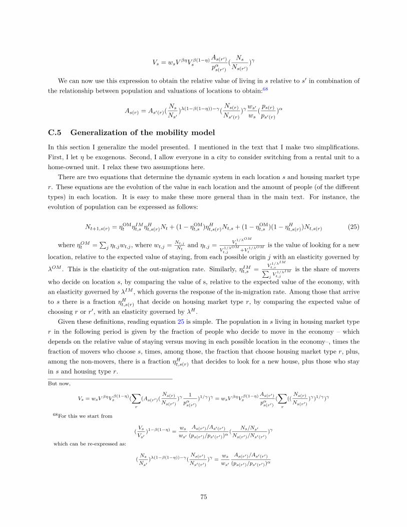
Vs = wsVβηV β(1−η)

s

As(r′)

pαs(r′)( NsNs(r′)

)γ

We can now use this expression to obtain the relative value of living in s relative to s′ in combination ofthe relationship between population and valuations of locations to obtain:68

As(r) = As′(r)(NsNs′

)λ(1−β(1−η))−γ(Ns(r)

Ns′(r))γws

′

ws(ps(r)

ps′(r))α

C.5 Generalization of the mobility model

In this section I generalize the model presented. I mentioned in the text that I make two simplifications.First, I let η be exogenous. Second, I allow everyone in a city to consider switching from a rental unit to ahome-owned unit. I relax these two assumptions here.

There are two equations that determine the dynamic system in each location s and housing market typer. These equations are the evolution of the value in each location and the amount of people (of the differenttypes) in each location. It is easy to make these more general than in the main text. For instance, theevolution of population can be expressed as follows:

Nt+1,s(r) = ηOMt ηIMt,s η

Ht,s(r)Nt + (1− ηOM

t,s )ηHt,s(r)Nt,s + (1− ηOMt,s )(1− ηHt,s(r))Nt,s(r) (25)

where ηOMt =∑j ηt,jwt,j , where wt,j = Nt,j

Ntand ηt,j = V

1/λOMt

V1/λOMt,j

+V 1/λOMt

is the value of looking for a new

location, relative to the expected value of staying, from each possible origin j with an elasticity governed by

λOM . This is the elasticity of the out-migration rate. Similarly, ηIMt,s = V1/λIMt,s∑jV

1/λIMt,j

is the share of movers

who decide on location s, by comparing the value of s, relative to the expected value of the economy, withan elasticity governed by λIM , which governs the response of the in-migration rate. Among those that arriveto s there is a fraction ηHt,s(r) that decide on housing market type r, by comparing the expected value ofchoosing r or r′, with an elasticity governed by λH .

Given these definitions, reading equation 25 is simple. The population in s living in housing market typer in the following period is given by the fraction of people who decide to move in the economy – whichdepends on the relative value of staying versus moving in each possible location in the economy–, times thefraction of movers who choose s, times, among those, the fraction that choose housing market type r, plus,among the non-movers, there is a fraction ηHt,s(r) that decides to look for a new house, plus those who stayin s and housing type r.

But now,

Vs = wsVβηV

β(1−η)s (

∑r

(As(r′)(Ns(r)

Ns(r′))γ

1pαs(r′)

)1/γ)γ = wsVβηV

β(1−η)s

As(r′)

pαs(r′)

(∑r

((Ns(r)

Ns(r′))γ)1/γ)γ

68For this we start from

(Vs

Vs′)1−β(1−η) =

ws

ws′

As(r′)/As′(r′)

(ps(r′)/ps′(r′))α(

Ns/Ns′

Ns(r′)/Ns′(r′))γ

which can be re-expressed as:

(Ns

Ns′)λ(1−β(1−η))−γ(

Ns(r′)

Ns′(r′))γ =

ws

ws′

As(r′)/As′(r′)

(ps(r′)/ps′(r′))α

75

As can be seen from this equation, the most complicated endogenous fraction to deal with is the fractionof people who move away from each possible origin. However, if this fraction is the same across locations,then, dealing with the dynamic equation is relatively simple as shown in the main text.

From Equation 25 it is also possible to recover the two formulations that are particularly easy to bringto the data. When ηOM

t is a constant, then the dynamics equation becomes:

Nt+1,s(r) = η(Vt,sVt

)1/λ(Vt,s(r)

Vt,s)1/γNt + (1− η)η̃(

Vt,s(r)

Vt,s)1/γNt,s + (1− η)(1− η̃)Nt,s(r)

In the main text I made the simplification η̃ = 1 which means that everyone considers all housing marketswithin locations every period.

Another interesting simplified version of the model delivers the following dynamics:

Nt+1,s(r) = η(Vt,sVt

)1/λ(Vt,s(r)

Vt,s)1/γNt + (1− η)Nt,s(r)

In this alternative, local residents are “locked” into their housing market type. This model generatesmore parsimonious dynamics in the housing market.

D Appendix: Figures and Tables

76

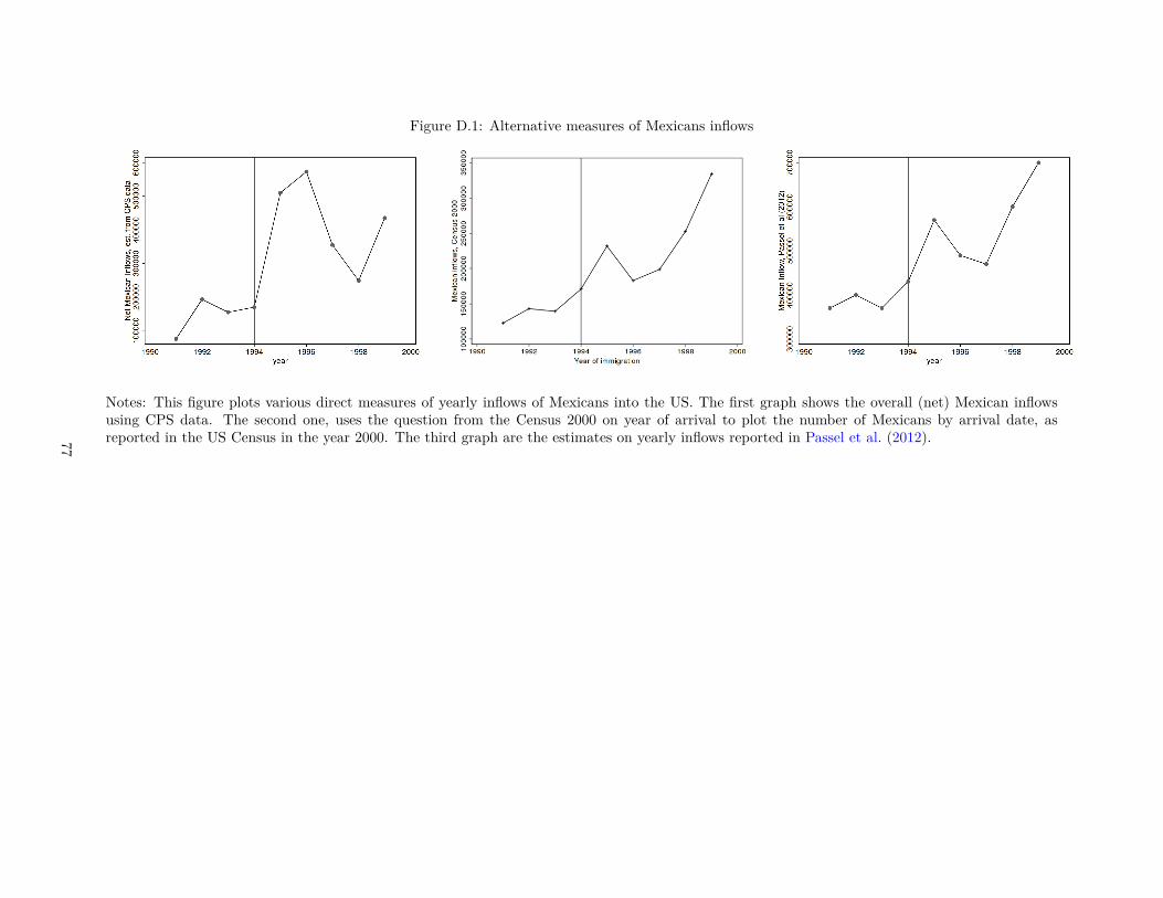
Figure D.1: Alternative measures of Mexicans inflows

Notes: This figure plots various direct measures of yearly inflows of Mexicans into the US. The first graph shows the overall (net) Mexican inflowsusing CPS data. The second one, uses the question from the Census 2000 on year of arrival to plot the number of Mexicans by arrival date, asreported in the US Census in the year 2000. The third graph are the estimates on yearly inflows reported in Passel et al. (2012).77

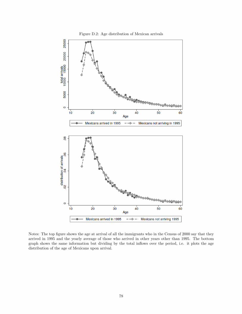
Figure D.2: Age distribution of Mexican arrivals

Notes: The top figure shows the age at arrival of all the immigrants who in the Census of 2000 say that theyarrived in 1995 and the yearly average of those who arrived in other years other than 1995. The bottomgraph shows the same information but dividing by the total inflows over the period, i.e. it plots the agedistribution of the age of Mexicans upon arrival.

78

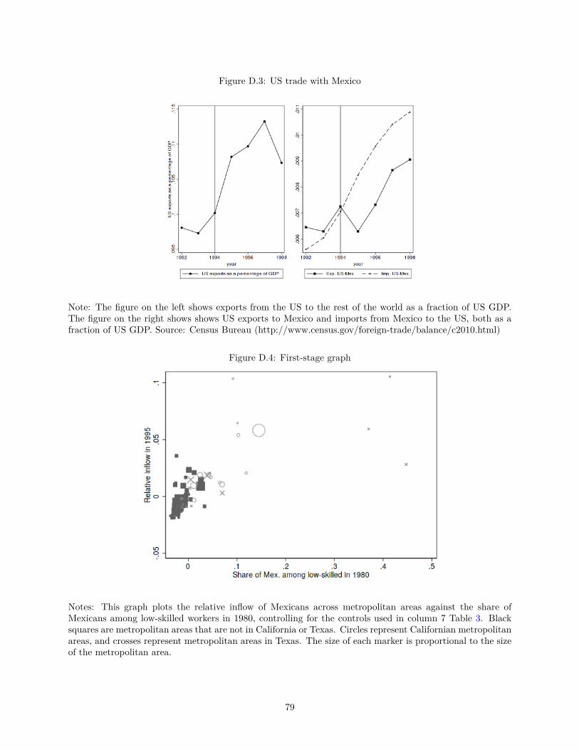
Figure D.3: US trade with Mexico

Note: The figure on the left shows exports from the US to the rest of the world as a fraction of US GDP.The figure on the right shows shows US exports to Mexico and imports from Mexico to the US, both as afraction of US GDP. Source: Census Bureau (http://www.census.gov/foreign-trade/balance/c2010.html)

Figure D.4: First-stage graph

Notes: This graph plots the relative inflow of Mexicans across metropolitan areas against the share ofMexicans among low-skilled workers in 1980, controlling for the controls used in column 7 Table 3. Blacksquares are metropolitan areas that are not in California or Texas. Circles represent Californian metropolitanareas, and crosses represent metropolitan areas in Texas. The size of each marker is proportional to the sizeof the metropolitan area.

79

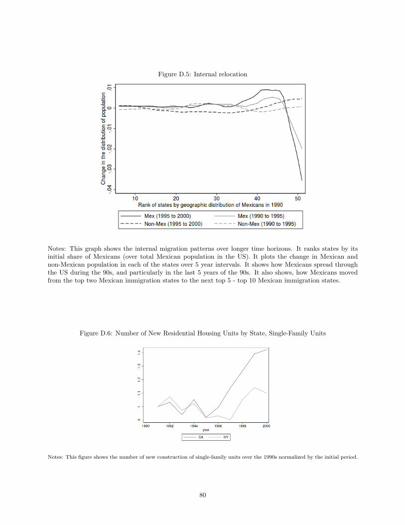
Figure D.5: Internal relocation

Notes: This graph shows the internal migration patterns over longer time horizons. It ranks states by itsinitial share of Mexicans (over total Mexican population in the US). It plots the change in Mexican andnon-Mexican population in each of the states over 5 year intervals. It shows how Mexicans spread throughthe US during the 90s, and particularly in the last 5 years of the 90s. It also shows, how Mexicans movedfrom the top two Mexican immigration states to the next top 5 - top 10 Mexican immigration states.

Figure D.6: Number of New Residential Housing Units by State, Single-Family Units

Notes: This figure shows the number of new construction of single-family units over the 1990s normalized by the initial period.

80

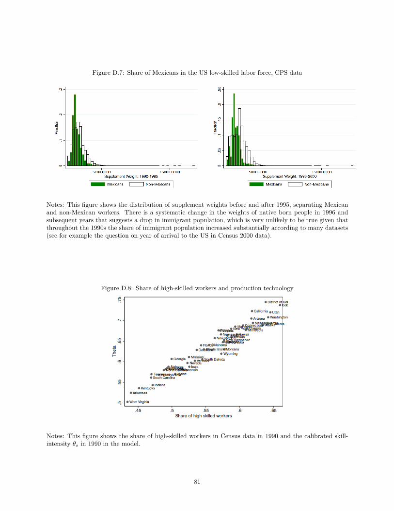
Figure D.7: Share of Mexicans in the US low-skilled labor force, CPS data

Notes: This figure shows the distribution of supplement weights before and after 1995, separating Mexicanand non-Mexican workers. There is a systematic change in the weights of native born people in 1996 andsubsequent years that suggests a drop in immigrant population, which is very unlikely to be true given thatthroughout the 1990s the share of immigrant population increased substantially according to many datasets(see for example the question on year of arrival to the US in Census 2000 data).

Figure D.8: Share of high-skilled workers and production technology

Notes: This figure shows the share of high-skilled workers in Census data in 1990 and the calibrated skill-intensity θs in 1990 in the model.

81

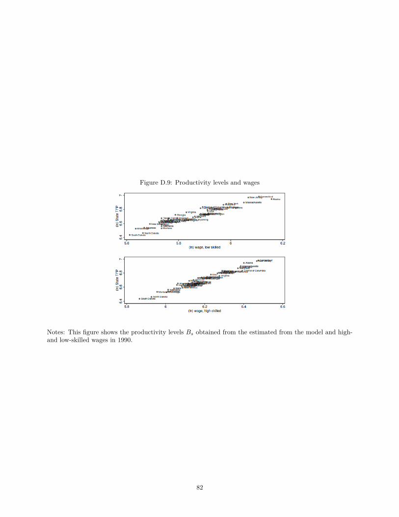
Figure D.9: Productivity levels and wages

Notes: This figure shows the productivity levels Bs obtained from the estimated from the model and high-and low-skilled wages in 1990.

82

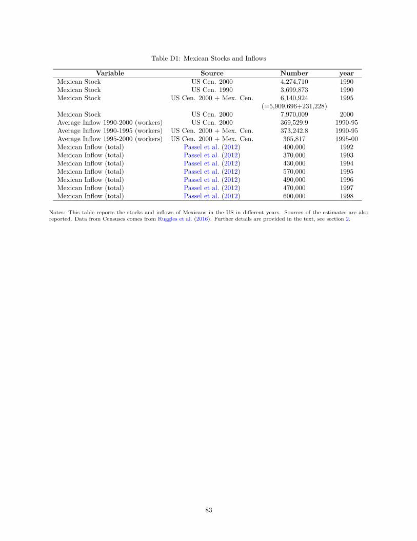
Table D1: Mexican Stocks and Inflows

Variable Source Number yearMexican Stock US Cen. 2000 4,274,710 1990Mexican Stock US Cen. 1990 3,699,873 1990Mexican Stock US Cen. 2000 + Mex. Cen. 6,140,924 1995

(=5,909,696+231,228)Mexican Stock US Cen. 2000 7,970,009 2000Average Inflow 1990-2000 (workers) US Cen. 2000 369,529.9 1990-95Average Inflow 1990-1995 (workers) US Cen. 2000 + Mex. Cen. 373,242.8 1990-95Average Inflow 1995-2000 (workers) US Cen. 2000 + Mex. Cen. 365,817 1995-00Mexican Inflow (total) Passel et al. (2012) 400,000 1992Mexican Inflow (total) Passel et al. (2012) 370,000 1993Mexican Inflow (total) Passel et al. (2012) 430,000 1994Mexican Inflow (total) Passel et al. (2012) 570,000 1995Mexican Inflow (total) Passel et al. (2012) 490,000 1996Mexican Inflow (total) Passel et al. (2012) 470,000 1997Mexican Inflow (total) Passel et al. (2012) 600,000 1998

Notes: This table reports the stocks and inflows of Mexicans in the US in different years. Sources of the estimates are alsoreported. Data from Censuses comes from Ruggles et al. (2016). Further details are provided in the text, see section 2.

83

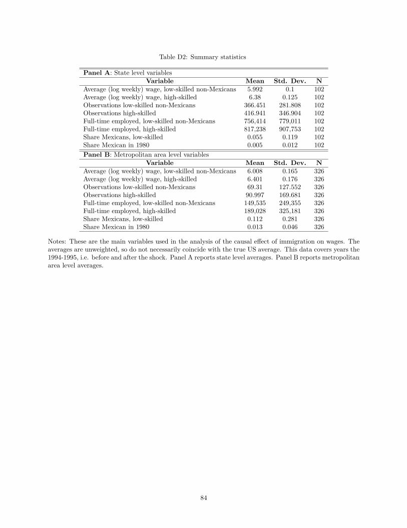
Table D2: Summary statistics

Panel A: State level variablesVariable Mean Std. Dev. N

Average (log weekly) wage, low-skilled non-Mexicans 5.992 0.1 102Average (log weekly) wage, high-skilled 6.38 0.125 102Observations low-skilled non-Mexicans 366.451 281.808 102Observations high-skilled 416.941 346.904 102Full-time employed, low-skilled non-Mexicans 756,414 779,011 102Full-time employed, high-skilled 817,238 907,753 102Share Mexicans, low-skilled 0.055 0.119 102Share Mexican in 1980 0.005 0.012 102Panel B: Metropolitan area level variables

Variable Mean Std. Dev. NAverage (log weekly) wage, low-skilled non-Mexicans 6.008 0.165 326Average (log weekly) wage, high-skilled 6.401 0.176 326Observations low-skilled non-Mexicans 69.31 127.552 326Observations high-skilled 90.997 169.681 326Full-time employed, low-skilled non-Mexicans 149,535 249,355 326Full-time employed, high-skilled 189,028 325,181 326Share Mexicans, low-skilled 0.112 0.281 326Share Mexican in 1980 0.013 0.046 326

Notes: These are the main variables used in the analysis of the causal effect of immigration on wages. Theaverages are unweighted, so do not necessarily coincide with the true US average. This data covers years the1994-1995, i.e. before and after the shock. Panel A reports state level averages. Panel B reports metropolitanarea level averages.

84

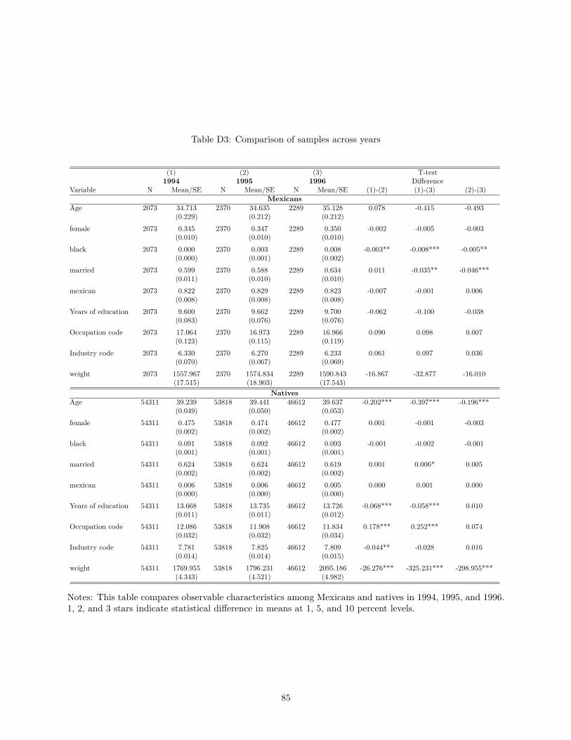
Table D3: Comparison of samples across years

(1) (2) (3) T-test1994 1995 1996 Difference

Variable N Mean/SE N Mean/SE N Mean/SE (1)-(2) (1)-(3) (2)-(3)Mexicans

Age 2073 34.713(0.229)

2370 34.635(0.212)

2289 35.128(0.212)

0.078 -0.415 -0.493

female 2073 0.345(0.010)

2370 0.347(0.010)

2289 0.350(0.010)

-0.002 -0.005 -0.003

black 2073 0.000(0.000)

2370 0.003(0.001)

2289 0.008(0.002)

-0.003** -0.008*** -0.005**

married 2073 0.599(0.011)

2370 0.588(0.010)

2289 0.634(0.010)

0.011 -0.035** -0.046***

mexican 2073 0.822(0.008)

2370 0.829(0.008)

2289 0.823(0.008)

-0.007 -0.001 0.006

Years of education 2073 9.600(0.083)

2370 9.662(0.076)

2289 9.700(0.076)

-0.062 -0.100 -0.038

Occupation code 2073 17.064(0.123)

2370 16.973(0.115)

2289 16.966(0.119)

0.090 0.098 0.007

Industry code 2073 6.330(0.070)

2370 6.270(0.067)

2289 6.233(0.069)

0.061 0.097 0.036

weight 2073 1557.967(17.515)

2370 1574.834(18.903)

2289 1590.843(17.543)

-16.867 -32.877 -16.010

NativesAge 54311 39.239

(0.049)53818 39.441

(0.050)46612 39.637

(0.053)-0.202*** -0.397*** -0.196***

female 54311 0.475(0.002)

53818 0.474(0.002)

46612 0.477(0.002)

0.001 -0.001 -0.003

black 54311 0.091(0.001)

53818 0.092(0.001)

46612 0.093(0.001)

-0.001 -0.002 -0.001

married 54311 0.624(0.002)

53818 0.624(0.002)

46612 0.619(0.002)

0.001 0.006* 0.005

mexican 54311 0.006(0.000)

53818 0.006(0.000)

46612 0.005(0.000)

0.000 0.001 0.000

Years of education 54311 13.668(0.011)

53818 13.735(0.011)

46612 13.726(0.012)

-0.068*** -0.058*** 0.010

Occupation code 54311 12.086(0.032)

53818 11.908(0.032)

46612 11.834(0.034)

0.178*** 0.252*** 0.074

Industry code 54311 7.781(0.014)

53818 7.825(0.014)

46612 7.809(0.015)

-0.044** -0.028 0.016

weight 54311 1769.955(4.343)

53818 1796.231(4.521)

46612 2095.186(4.982)

-26.276*** -325.231*** -298.955***

Notes: This table compares observable characteristics among Mexicans and natives in 1994, 1995, and 1996.1, 2, and 3 stars indicate statistical difference in means at 1, 5, and 10 percent levels.

85

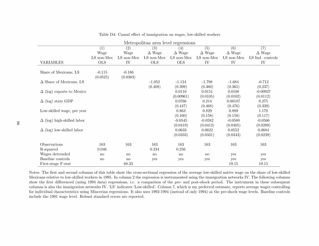
Table D4: Causal effect of immigration on wages, low-skilled workers

Metropolitan area level regressions(1) (2) (3) (4) (5) (6) (7)





∆ (log) exports to Mexico 0.0110 0.0151 0.0108 -0.00937(0.00961) (0.0105) (0.0102) (0.0112)

∆ (log) state GDP 0.0766 0.214 0.00187 0.275(0.447) (0.468) (0.476) (0.339)

Low-skilled wage, pre year 0.863 0.829 0.889 1.178(0.160) (0.158) (0.158) (0.117)

∆ (log) high-skilled labor -0.0545 -0.0582 -0.0580 -0.0566(0.0419) (0.0412) (0.0405) (0.0289)

∆ (log) low-skilled labor 0.0633 0.0622 0.0552 0.0684(0.0333) (0.0331) (0.0343) (0.0239)

Observations 163 163 163 163 163 163 163R-squared 0.046 0.234 0.256Wages detrended no no no no no yes yesBaseline controls no no yes yes yes yes yesFirst-stage F-stat 68.33 19.15 19.15

Notes: The first and second columns of this table show the cross-sectional regression of the average low-skilled native wage on the share of low-skilledMexicans relative to low-skilled workers in 1995. In column 2 the regression is instrumented using the immigration networks IV. The following columnsshow the first differenced (using 1994 data) regressions, i.e. a comparison of the pre- and post-shock period. The instrument in these subsequentcolumns is also the immigration networks IV. ‘LS’ indicates ‘Low-skilled’. Column 7, which is my preferred estimate, reports average wages controllingfor individual characteristics using Mincerian regressions. It also uses 1992-1994 (instead of only 1994) as the pre-shock wage levels. Baseline controlsinclude the 1991 wage level. Robust standard errors are reported.

86

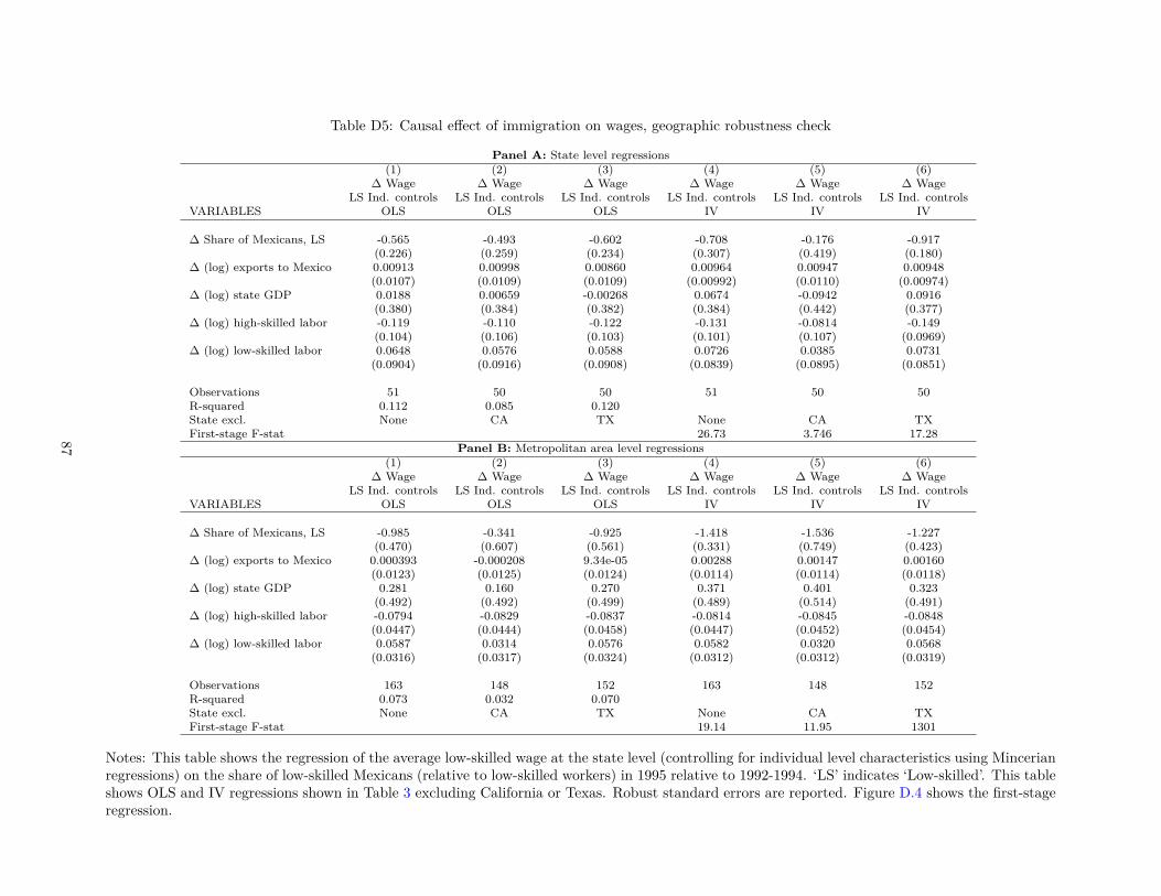
Table D5: Causal effect of immigration on wages, geographic robustness check

Panel A: State level regressions(1) (2) (3) (4) (5) (6)

∆ Wage ∆ Wage ∆ Wage ∆ Wage ∆ Wage ∆ WageLS Ind. controls LS Ind. controls LS Ind. controls LS Ind. controls LS Ind. controls LS Ind. controls

VARIABLES OLS OLS OLS IV IV IV

∆ Share of Mexicans, LS -0.565 -0.493 -0.602 -0.708 -0.176 -0.917(0.226) (0.259) (0.234) (0.307) (0.419) (0.180)

∆ (log) exports to Mexico 0.00913 0.00998 0.00860 0.00964 0.00947 0.00948(0.0107) (0.0109) (0.0109) (0.00992) (0.0110) (0.00974)

∆ (log) state GDP 0.0188 0.00659 -0.00268 0.0674 -0.0942 0.0916(0.380) (0.384) (0.382) (0.384) (0.442) (0.377)

∆ (log) high-skilled labor -0.119 -0.110 -0.122 -0.131 -0.0814 -0.149(0.104) (0.106) (0.103) (0.101) (0.107) (0.0969)

∆ (log) low-skilled labor 0.0648 0.0576 0.0588 0.0726 0.0385 0.0731(0.0904) (0.0916) (0.0908) (0.0839) (0.0895) (0.0851)

Observations 51 50 50 51 50 50R-squared 0.112 0.085 0.120State excl. None CA TX None CA TXFirst-stage F-stat 26.73 3.746 17.28

Panel B: Metropolitan area level regressions(1) (2) (3) (4) (5) (6)

∆ Wage ∆ Wage ∆ Wage ∆ Wage ∆ Wage ∆ WageLS Ind. controls LS Ind. controls LS Ind. controls LS Ind. controls LS Ind. controls LS Ind. controls

VARIABLES OLS OLS OLS IV IV IV

∆ Share of Mexicans, LS -0.985 -0.341 -0.925 -1.418 -1.536 -1.227(0.470) (0.607) (0.561) (0.331) (0.749) (0.423)

∆ (log) exports to Mexico 0.000393 -0.000208 9.34e-05 0.00288 0.00147 0.00160(0.0123) (0.0125) (0.0124) (0.0114) (0.0114) (0.0118)

∆ (log) state GDP 0.281 0.160 0.270 0.371 0.401 0.323(0.492) (0.492) (0.499) (0.489) (0.514) (0.491)



Observations 163 148 152 163 148 152R-squared 0.073 0.032 0.070State excl. None CA TX None CA TXFirst-stage F-stat 19.14 11.95 1301

Notes: This table shows the regression of the average low-skilled wage at the state level (controlling for individual level characteristics using Mincerianregressions) on the share of low-skilled Mexicans (relative to low-skilled workers) in 1995 relative to 1992-1994. ‘LS’ indicates ‘Low-skilled’. This tableshows OLS and IV regressions shown in Table 3 excluding California or Texas. Robust standard errors are reported. Figure D.4 shows the first-stageregression.

87

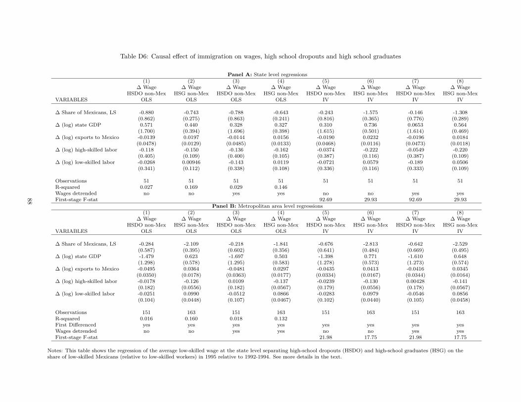
Table D6: Causal effect of immigration on wages, high school dropouts and high school graduates


∆ Wage ∆ Wage ∆ Wage ∆ Wage ∆ Wage ∆ Wage ∆ Wage ∆ WageHSDO non-Mex HSG non-Mex HSDO non-Mex HSG non-Mex HSDO non-Mex HSG non-Mex HSDO non-Mex HSG non-Mex

VARIABLES OLS OLS OLS OLS IV IV IV IV

∆ Share of Mexicans, LS -0.880 -0.743 -0.788 -0.643 -0.243 -1.575 -0.146 -1.308(0.862) (0.275) (0.863) (0.241) (0.816) (0.365) (0.776) (0.289)

∆ (log) state GDP 0.571 0.440 0.328 0.327 0.310 0.736 0.0653 0.564(1.700) (0.394) (1.696) (0.398) (1.615) (0.501) (1.614) (0.469)

∆ (log) exports to Mexico -0.0139 0.0197 -0.0144 0.0156 -0.0190 0.0232 -0.0196 0.0184(0.0478) (0.0129) (0.0485) (0.0133) (0.0468) (0.0116) (0.0473) (0.0118)

∆ (log) high-skilled labor -0.118 -0.150 -0.136 -0.162 -0.0374 -0.222 -0.0549 -0.220(0.405) (0.109) (0.400) (0.105) (0.387) (0.116) (0.387) (0.109)

∆ (log) low-skilled labor -0.0268 0.00946 -0.143 0.0119 -0.0721 0.0579 -0.189 0.0506(0.341) (0.112) (0.338) (0.108) (0.336) (0.116) (0.333) (0.109)

Observations 51 51 51 51 51 51 51 51R-squared 0.027 0.169 0.029 0.146Wages detrended no no yes yes no no yes yesFirst-stage F-stat 92.69 29.93 92.69 29.93


∆ Wage ∆ Wage ∆ Wage ∆ Wage ∆ Wage ∆ Wage ∆ Wage ∆ WageHSDO non-Mex HSG non-Mex HSDO non-Mex HSG non-Mex HSDO non-Mex HSG non-Mex HSDO non-Mex HSG non-Mex



∆ (log) state GDP -1.479 0.623 -1.697 0.503 -1.398 0.771 -1.610 0.648(1.298) (0.578) (1.295) (0.583) (1.278) (0.573) (1.273) (0.574)

∆ (log) exports to Mexico -0.0495 0.0364 -0.0481 0.0297 -0.0435 0.0413 -0.0416 0.0345(0.0350) (0.0178) (0.0363) (0.0177) (0.0334) (0.0167) (0.0344) (0.0164)

∆ (log) high-skilled labor -0.0178 -0.126 0.0109 -0.137 -0.0239 -0.130 0.00428 -0.141(0.182) (0.0556) (0.182) (0.0567) (0.179) (0.0556) (0.178) (0.0567)

∆ (log) low-skilled labor -0.0251 0.0990 -0.0512 0.0866 -0.0283 0.0979 -0.0546 0.0856(0.104) (0.0448) (0.107) (0.0467) (0.102) (0.0440) (0.105) (0.0458)

Observations 151 163 151 163 151 163 151 163R-squared 0.016 0.160 0.018 0.132First Differenced yes yes yes yes yes yes yes yesWages detrended no no yes yes no no yes yesFirst-stage F-stat 21.98 17.75 21.98 17.75

Notes: This table shows the regression of the average low-skilled wage at the state level separating high-school dropouts (HSDO) and high-school graduates (HSG) on theshare of low-skilled Mexicans (relative to low-skilled workers) in 1995 relative to 1992-1994. See more details in the text.

88

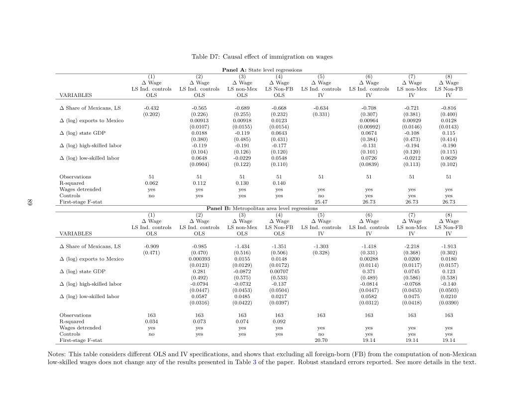
Table D7: Causal effect of immigration on wages


∆ Wage ∆ Wage ∆ Wage ∆ Wage ∆ Wage ∆ Wage ∆ Wage ∆ WageLS Ind. controls LS Ind. controls LS non-Mex LS Non-FB LS Ind. controls LS Ind. controls LS non-Mex LS Non-FB




∆ (log) state GDP 0.0188 -0.119 0.0643 0.0674 -0.108 0.115(0.380) (0.485) (0.431) (0.384) (0.473) (0.414)


∆ (log) low-skilled labor 0.0648 -0.0229 0.0548 0.0726 -0.0212 0.0629(0.0904) (0.122) (0.110) (0.0839) (0.113) (0.102)

Observations 51 51 51 51 51 51 51 51R-squared 0.062 0.112 0.130 0.140Wages detrended yes yes yes yes yes yes yes yesControls no yes yes yes no yes yes yesFirst-stage F-stat 25.47 26.73 26.73 26.73


∆ Wage ∆ Wage ∆ Wage ∆ Wage ∆ Wage ∆ Wage ∆ Wage ∆ WageLS Ind. controls LS Ind. controls LS non-Mex LS Non-FB LS Ind. controls LS Ind. controls LS non-Mex LS Non-FB




∆ (log) state GDP 0.281 -0.0872 0.00707 0.371 0.0745 0.123(0.492) (0.575) (0.533) (0.489) (0.586) (0.538)



Observations 163 163 163 163 163 163 163 163R-squared 0.034 0.073 0.074 0.092Wages detrended yes yes yes yes yes yes yes yesControls no yes yes yes no yes yes yesFirst-stage F-stat 20.70 19.14 19.14 19.14

Notes: This table considers different OLS and IV specifications, and shows that excluding all foreign-born (FB) from the computation of non-Mexicanlow-skilled wages does not change any of the results presented in Table 3 of the paper. Robust standard errors reported. See more details in the text.

89

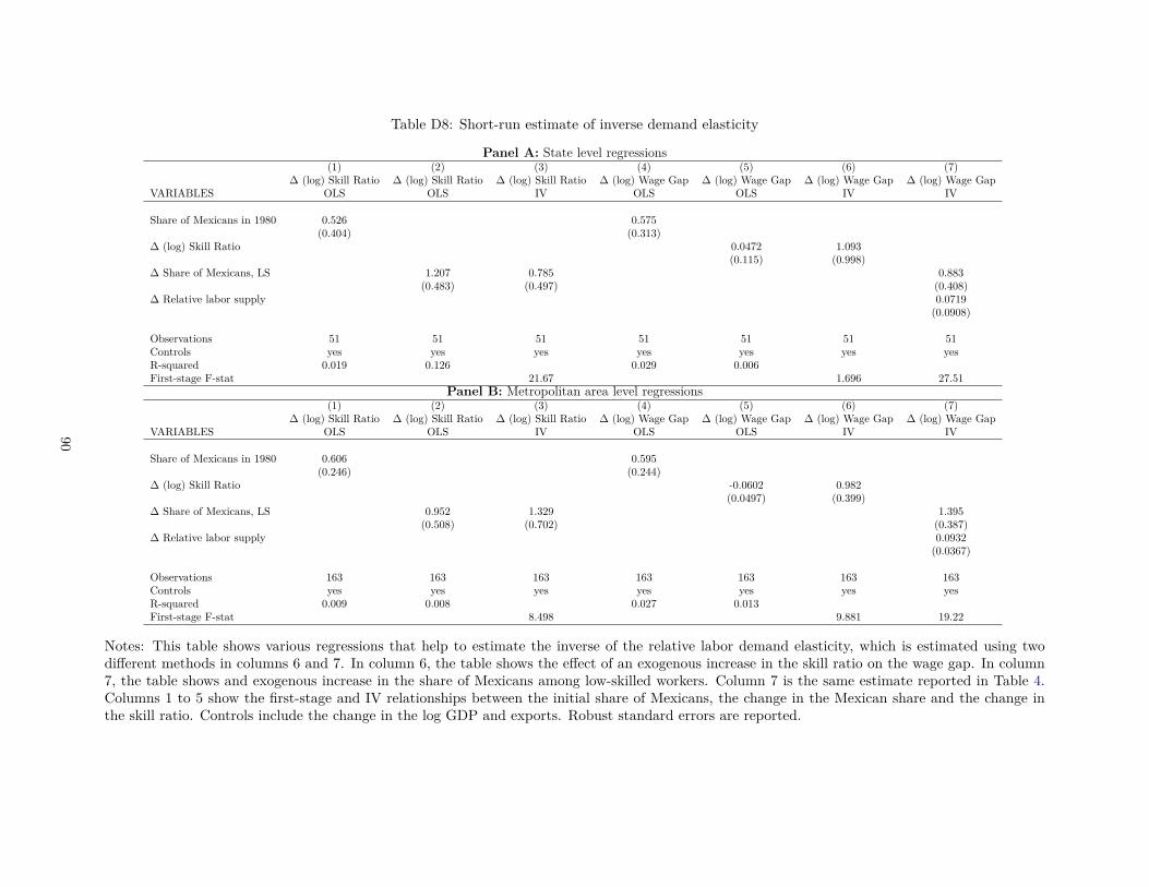
Table D8: Short-run estimate of inverse demand elasticity

Panel A: State level regressions(1) (2) (3) (4) (5) (6) (7)

∆ (log) Skill Ratio ∆ (log) Skill Ratio ∆ (log) Skill Ratio ∆ (log) Wage Gap ∆ (log) Wage Gap ∆ (log) Wage Gap ∆ (log) Wage GapVARIABLES OLS OLS IV OLS OLS IV IV

Share of Mexicans in 1980 0.526 0.575(0.404) (0.313)

∆ (log) Skill Ratio 0.0472 1.093(0.115) (0.998)


∆ Relative labor supply 0.0719(0.0908)

Observations 51 51 51 51 51 51 51Controls yes yes yes yes yes yes yesR-squared 0.019 0.126 0.029 0.006First-stage F-stat 21.67 1.696 27.51

Panel B: Metropolitan area level regressions(1) (2) (3) (4) (5) (6) (7)

∆ (log) Skill Ratio ∆ (log) Skill Ratio ∆ (log) Skill Ratio ∆ (log) Wage Gap ∆ (log) Wage Gap ∆ (log) Wage Gap ∆ (log) Wage GapVARIABLES OLS OLS IV OLS OLS IV IV

Share of Mexicans in 1980 0.606 0.595(0.246) (0.244)

∆ (log) Skill Ratio -0.0602 0.982(0.0497) (0.399)


∆ Relative labor supply 0.0932(0.0367)

Observations 163 163 163 163 163 163 163Controls yes yes yes yes yes yes yesR-squared 0.009 0.008 0.027 0.013First-stage F-stat 8.498 9.881 19.22

Notes: This table shows various regressions that help to estimate the inverse of the relative labor demand elasticity, which is estimated using twodifferent methods in columns 6 and 7. In column 6, the table shows the effect of an exogenous increase in the skill ratio on the wage gap. In column7, the table shows and exogenous increase in the share of Mexicans among low-skilled workers. Column 7 is the same estimate reported in Table 4.Columns 1 to 5 show the first-stage and IV relationships between the initial share of Mexicans, the change in the Mexican share and the change inthe skill ratio. Controls include the change in the log GDP and exports. Robust standard errors are reported.

90

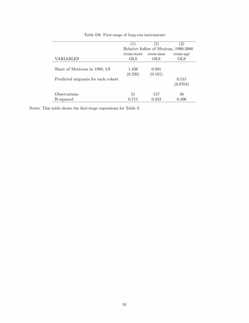
Table D9: First-stage of long-run instruments

(1) (2) (3)Relative Inflow of Mexican, 1990-2000cross-state cross-msa cross-age

VARIABLES OLS OLS OLS


Predicted migrants for each cohort 0.515(0.0704)

Observations 51 157 46R-squared 0.715 0.353 0.496

Notes: This table shows the first-stage regressions for Table 9.

91

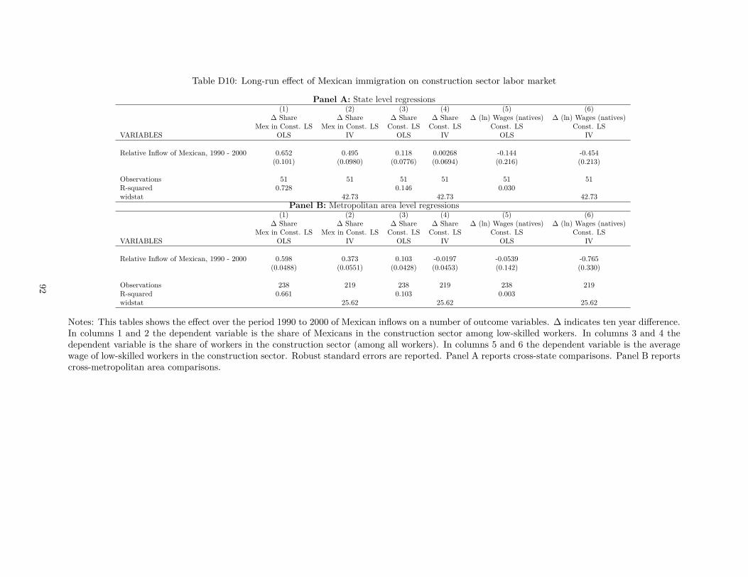
Table D10: Long-run effect of Mexican immigration on construction sector labor market

Panel A: State level regressions(1) (2) (3) (4) (5) (6)

∆ Share ∆ Share ∆ Share ∆ Share ∆ (ln) Wages (natives) ∆ (ln) Wages (natives)Mex in Const. LS Mex in Const. LS Const. LS Const. LS Const. LS Const. LS

VARIABLES OLS IV OLS IV OLS IV

Relative Inflow of Mexican, 1990 - 2000 0.652 0.495 0.118 0.00268 -0.144 -0.454(0.101) (0.0980) (0.0776) (0.0694) (0.216) (0.213)

Observations 51 51 51 51 51 51R-squared 0.728 0.146 0.030widstat 42.73 42.73 42.73

Panel B: Metropolitan area level regressions(1) (2) (3) (4) (5) (6)

∆ Share ∆ Share ∆ Share ∆ Share ∆ (ln) Wages (natives) ∆ (ln) Wages (natives)Mex in Const. LS Mex in Const. LS Const. LS Const. LS Const. LS Const. LS

VARIABLES OLS IV OLS IV OLS IV

Relative Inflow of Mexican, 1990 - 2000 0.598 0.373 0.103 -0.0197 -0.0539 -0.765(0.0488) (0.0551) (0.0428) (0.0453) (0.142) (0.330)

Observations 238 219 238 219 238 219R-squared 0.661 0.103 0.003widstat 25.62 25.62 25.62

Notes: This tables shows the effect over the period 1990 to 2000 of Mexican inflows on a number of outcome variables. ∆ indicates ten year difference.In columns 1 and 2 the dependent variable is the share of Mexicans in the construction sector among low-skilled workers. In columns 3 and 4 thedependent variable is the share of workers in the construction sector (among all workers). In columns 5 and 6 the dependent variable is the averagewage of low-skilled workers in the construction sector. Robust standard errors are reported. Panel A reports cross-state comparisons. Panel B reportscross-metropolitan area comparisons.

92

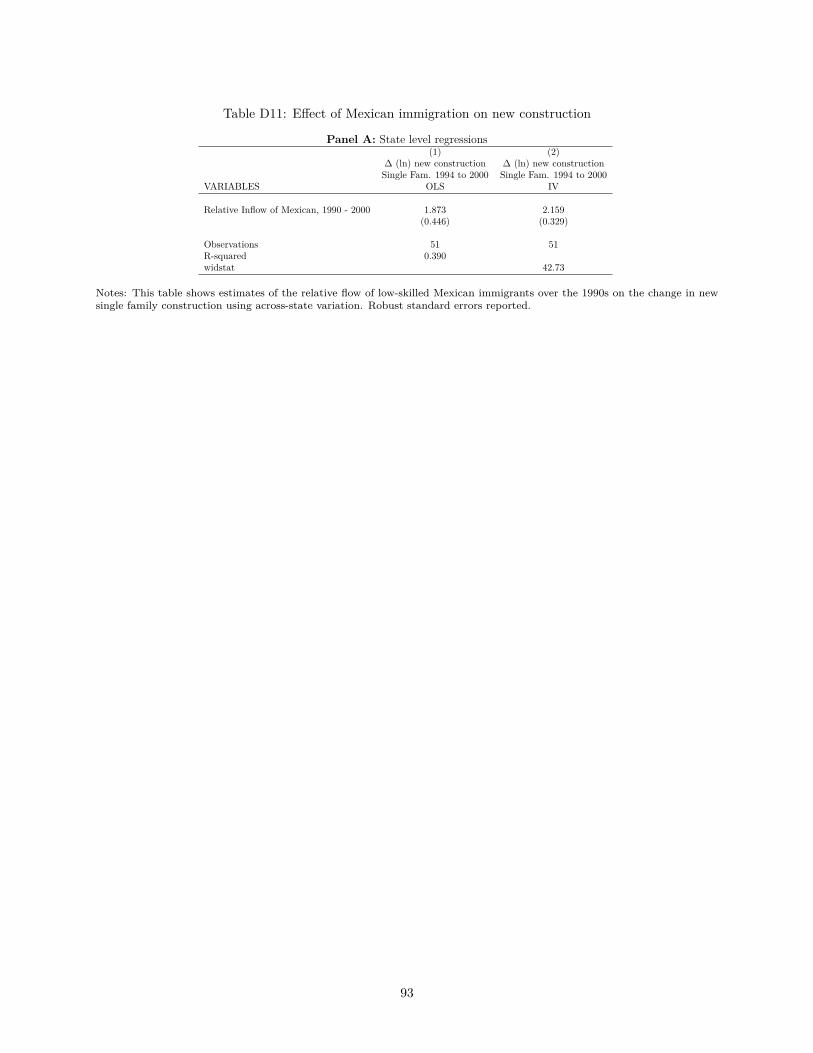
Table D11: Effect of Mexican immigration on new construction

Panel A: State level regressions(1) (2)

∆ (ln) new construction ∆ (ln) new constructionSingle Fam. 1994 to 2000 Single Fam. 1994 to 2000

VARIABLES OLS IV

Relative Inflow of Mexican, 1990 - 2000 1.873 2.159(0.446) (0.329)

Observations 51 51R-squared 0.390widstat 42.73

Notes: This table shows estimates of the relative flow of low-skilled Mexican immigrants over the 1990s on the change in newsingle family construction using across-state variation. Robust standard errors reported.

93

Documents

Evidence from the Mexican Peso crisis