Is there a contemporaneous relation

between exchange rates and stock prices?

Evidence from decisions to allow the Mexican Peso and Thai Baht to float

Kathryn L. Dewenter

Robert C. Higgins

Timothy T. Simin*

March 2002

Abstract

This paper estimates short horizon exchange rate sensitivity with an event study methodology. We look at stock price reactions to very large, unexpected exchange rate changes: the decisions to allow the Mexican peso and Thai baht to float. For both events, we find evidence of a statistically and economically significant contemporaneous relation. Our findings are consistent with the premise that the inability of much of the prior research to observe a contemporaneous relation between exchange rates and company value is due to methodological issues. JEL: F3, F4, F2 * Dewenter and Higgins are from the Department of Finance, Box 353200, University of Washington, Seattle, WA 98195. Simin is from the Finance Department, Smeal School of Business, 609 Business Administration Building, Penn State University, University Park, PA 16802. Corresponding author is Dewenter at dewe@u.washington.edu. We would like to thank Chris Anderson, Soenke Bartram, David Haushalter, Ulrich Hommel, and seminar participants at the FMA meetings (2000), U. of Kansas, Penn State, U. of Washington, and Wharton (Multinational Management) for helpful suggestions. All remaining errors are our own.

29

A basic tenant of international finance is that changes in exchange rates affect firm

values. Thus the home currency value of foreign-denominated monetary assets and liabilities

varies with changes in the nominal exchange rate, while the value of nonmonetary assets and

liabilities is sensitive to changes in the real rate, or equivalently to deviations from purchasing

power parity (see Adler and Dumas 1984, Froot and Rogoff 1995). International finance

textbooks carry the same message, often devoting multiple chapters to measuring and managing

corporate foreign exchange exposure (see Eun and Resnick 2001 and Shapiro 1999). Surveys of

corporate behavior further underline the perceived importance of the topic to practitioners,

reporting that firms devote considerable resources to determining and managing their currency

exposures (see Graham and Harvey 2000, Geczy, et. al. 1997, Phillips 1995, and Price

Waterhouse 1995).

Yet despite the acknowledged importance of foreign currency exposure in theory and

practice, repeated empirical attempts to observe the expected relation between exchange rate

changes and firm value have been only modestly successful. Beginning with Adler and Dumas

(1983), economists have been attempting to measure firms’ exchange rate exposure by

regressing firm stock returns against exchange rate changes, controlling for various other factors.

Contrary to expectations, most studies find little evidence of a contemporaneous relation

between exchange rate changes and stock returns. For example, Jorion’s (1990) study of US

firms finds that only 5% of his sample firms have significant exchange rate elasticity estimates.1

Three broad explanations for this puzzling lack of evidence exist. One is that companies

may use financial derivatives and operating hedges to minimize net exposure. Foreign exchange

rate risk may therefore exist in principle, but companies manage it so successfully that firm value

is virtually immunized from exchange rate changes. Evidence supporting this conjecture is

mixed. Allayannis and Ofek (1998) find firms that use derivatives have smaller exposure

estimates than other firms, although they cannot infer causality. Chow, Lee and Solt (1997a)

also find tangential evidence consistent with the efficacy of hedging when they observe that

exposure estimates at longer horizons exceed those at shorter horizons, a finding consistent with

1 More recent studies of non-US firms appear to find stronger evidence of a contemporaneous exchange rate exposure. See Chow and Chen (1998) and He and Ng (1998) for studies of Japanese firms, Priestley and Odegaard (2001) for a study of Norwegian firms, and Chamberlain, Howe, and Popper (1997) for a comparison of US and Japanese banks.

30

the use of low cost financial instruments to hedge short-term exposure. However, Guay and

Kothari (2001) conclude that firms’ derivatives positions are consistent with speculation as well

as with risk management, while Hentschel and Kothari (2001) observe that derivative use does

not appear to reduce corporate risk. A recent study by Linck (1999) provides evidence that

operational hedging may be more effective, arguing that the net cash flow effects of currency

changes appear to be quite small.

A second explanation is that investors may lack sufficient information about the currency

exposures companies face to respond quickly to exchange rate changes. Instead, their reaction is

delayed until the rate changes affect observable firm cash flows. Existing empirical work thus

errs by seeking a contemporaneous relation between exchange rate changes and firm value.

Bartov and Bodnar (1994) report evidence consistent with this explanation when they show that

lagged values of the exchange rate and subsequent earnings announcements have stronger

explanatory power for stock returns than does the contemporaneous exchange rate. However,

this explanation rests on two awkward premises. First, corporate reporting about currency

exposures must be so fragmentary or opaque that even knowledgeable investors are unable to

form expectations about the sign and magnitude of firm exposure. Second, investors must also

be unable to form opinions about company exposures by observing past relations between

exchange rate changes and firm cash flows. This second premise might hold if company

currency exposures changed rapidly in size and sign over time, but this appears not to be the

case. Indeed, Bartov and Bodnar’s (1994) finding of a diminishing importance of lagged

currency changes relative to contemporaneous ones suggests that exposures are stable over time

and that investor learning does occur.

The third explanation of the puzzle is that existing empirical tests suffer from

methodological weaknesses and data limitations that severely compromise their power. Some

studies argue that sample selection problems are to blame, that sample firms do not have

sufficient exposure to the chosen exchange rate or that the samples mingle firms with positive

and negative exposures, thereby obscuring any evidence of an average effect. After refining

their samples, Bartov and Bodner (1994) and Choi and Prasad (1995) find stronger, but still

weak, evidence of a short-run relation between stock returns and exchange rate changes.

Others argue that the problem lies with the exchange rate measure. Most prior studies

test the sensitivity of firm returns to changes in a trade-weighted value of the dollar. Yet it is

31

doubtful that the exchange rate exposure of any given company matches the trade weights used

to measure the exchange rate, thereby weakening the correlation between firm value and changes

in the exchange rate index. Moreover, the trade-weighted value of the dollar changes very little

from month to month over most of the time periods covered in earlier studies, making it difficult

for investors to distinguish between signal and noise in the observed changes.2 Consistent with

this perspective, studies using bilateral exchange rates, particularly those with non-US samples,

tend to report stronger evidence of short-run currency exposure.3

A third methodological criticism is that the relation between currency changes and stock

returns may not be linear, with the true relation depending in complex ways on the direction of

the currency movement (Choi and Prasad 1995), the size of the movement (Doidge, Griffin,

Williamson 2000), and possibly the nature of the exposure itself (Williamson 2001). Attempts to

capture such nonlinearities have yielded mixed results, with a common finding of stronger

exposure estimates during periods of larger currency movements.

This paper considers the currency exposure puzzle from a new perspective. We report

results of an event study of the effect of large, unexpected changes in bilateral exchange rates on

the stock prices of firms with known operations in the foreign country. We look at two different

events: Mexico’s float of the peso in December 1994, and Thailand’s float of the baht in July

1997. (See the Appendix for a summary of these events.) Both events involved large,

unexpected exchange rate changes, 35.0 percent and 16.6 percent, respectively over a seven-day

window.4

An event study methodology appears particularly well suited to study exchange rate

exposure. By concentrating on sudden, large exchange rate movements, we greatly increase the

2 For example, during the 1980s, the average of the absolute value of monthly changes in the International Monetary Funds’ (IMF) nominal and real trade weighted dollar indices are 1.7 percent and 1.5 percent, respectively. It is difficult to envision stock prices responding to 1-2 percent monthly changes in exchange rates that could be random draws from a stable distribution, i.e. noise. 3 Some recent papers that do examine exchange rate exposure with bilateral rates are Bailey and Chung (1995), Choi, Hiraki, and Takezawa (1998), Khoo (1994), and Priestley and Odegaard (2001) and Williamson (2001). Khoo, looking at mining firms in Australia, finds only weak evidence of a relation with bi-lateral exchange rates. Bailey and Chung, Choi, Hiraki and Takezawa, and Priestley and Odegaard, find stronger evidence in their studies of industry portfolios from Mexico, Japan, and Norway, respectively. Williamson gets significant exposure estimates for US and Japanese auto firms. 4 While well-publicized macroeconomic problems in these countries may have led many investors to expect a devaluation, they could not have known with certainty if or when it would occur. Chowdry and Goyal (2000), in referring to the Asia financial crisis, note “…no exaggeration to say that the crisis caught everyone unawares with rare warning signals from academic quarters.” To the extent that the events were anticipated, the power of our tests is weakened.

32

power of the tests. By limiting the samples to firms with operations in Mexico and Thailand, we

can be certain that all sample firms are exposed to the appropriate bilateral exchange rate. By

testing for volume and volatility effects (in addition to looking at individual firm and sample

average returns), we are able to provide evidence that is untainted by any downward bias caused

by the commingling of returns for firms with positive and negative exposures. And by observing

exchange rate exposure at a point in time, we avoid any non-linear measurement problems

caused by imposing fixed coefficient estimates over long periods.

Our objective is to answer two questions: do firms with foreign exchange exposure

evidence statistically significant stock price reactions immediately following currency float

announcements, and are the reactions economically significant? We find strong evidence of a

contemporaneous relation between exchange rates and the stock prices of US multinational firms

in both samples. Further tests suggest that the relation is economically as well as statistically

significant. For example, across firms with positive exposure estimates, the average abnormal

return over a 2-day event window is 3.72 percent for the Mexico sample and 2.16 percent for the

Thai sample.

Consistent with received theory and practice, our evidence suggests that firms do face

significant contemporaneous exchange rate risk, and that they do not fully hedge this exposure --

although we cannot rule out the possibility that hedging may reduce it. The evidence further

suggests that prices do respond rapidly to exchange rate movements. Finally our results suggest

that the failure of prior studies to find a contemporaneous price response to exchange rate

movements is most likely due to methodological problems that compromise the power of the

tests employed.

The paper proceeds as follows. In section I, we discuss our sample selection criteria and

our methods for calculating stock price reactions on the event dates. In section II, we present the

statistical tests. In section III, we discuss the economic significance and interpretation of the

results, and in section IV, we conclude.

I. Samples, Measures, and Tests of Significance

A. Samples

Sample firms for the Mexico event come from the 2000 Standard and Poor’s Compustat

Business Information file. We select US incorporated firms that report both domestic sales and

33

some information about sales or assets in Mexico (Compustat Code: 63). 5 The Business

Information file provides data on sales, profits, depreciation, capital expenditures, and

identifiable assets by geographic region.

Financial Accounting Standard no. 14, published in December 1976, requires U.S.

companies to disclose geographical information about foreign operations if such operations

account for more than 10 percent of total operations. In addition, a number of companies

voluntarily report geographical information even when they do not meet this threshold. Because

company policies regarding transfer prices and cost allocations make the distinction between

foreign and domestic sales and profits somewhat arbitrary, the Financial Accounting Standards

Board allows companies considerable latitude in interpreting their geographical reporting

requirements. In addition, the firms are not required to disclose the exact nature of their foreign

operations, for example, whether foreign assets are used for full-scale production or final

assembly. As a result, for the firms that chose to report foreign assets or sales, we can reliably

identify where a firm operates, but not exactly what its operations are.

The Compustat data set does not provide a geographic code for Thailand. For the Thai

baht event, we include companies that list affiliates or subsidiaries in Thailand in the 1997

Directory of Corporate Affiliations.6 The daily firm and market returns and market capitalization

for all firms come from the 2000 Center for Research of Stock Prices (CRSP) database. For

these firms we extract foreign sales, total sales, and sales to Asia (Compustat Codes: 20, 21, 22,

40, 41) from the Compustat Business Information file when available.

Table I provides descriptive statistics for the two samples. The table shows that our total

sample sizes are 316 for Mexico and 75 for Thailand. These samples tend to include large firms,

with average market capitalization of $3.0 billion for the Mexico sample and $19.7 billion for the

Thai sample. Approximately one-third (two-thirds) of the firms in the Mexican (Thai) sample are

from the largest decile of firms in the CRSP size-based rankings (based on year end market

capitalization). The mean ratio of total foreign sales to total sales equals 29.4 percent and 45.4

percent for the Mexico and Thai samples, respectively. The correlation between market

5 We include firms providing data for Mexico that are combined with data for regions that are not applicable to this study. 6 This source has the subtitle “Who owns Whom.” We rely on 1997 Volume 3, US Public Companies.

34

capitalization and the ratio of foreign/total sales is positive, but not strong, at 19.6 and 13.9

percent for the Mexico and Thai samples, respectively.

B. Tests of statistical significance

Event studies adopt two approaches to determine whether or not stock prices react to a

specific event: event parameter regressions and abnormal returns. We use both in this study.

The typical event parameter study regresses individual firm (or portfolio) returns against returns

for the home stock index and an event dummy variable (D) set equal to one over the event

window. A number of event studies further adjust returns for additional factors beyond the home

market index. Campbell, Lo, and MacKinlay (1997) note that the gains from this strategy, in

terms of reducing variance, are greatest when “the sample firms have a common characteristic.”

The obvious common characteristic across our sample firms is that they operate in either Mexico

or Thailand. Including the foreign stock market index in the regressions controls for general

market conditions and reactions in those countries, thereby allowing us to more precisely

measure firm specific abnormal returns due to an event, such as the currency float decision.

The empirical specification is:

1 2 3it i i mt i ft i itR R R Dα β β β ε= + + + + (1)

Where Rit is the return on the stock, or portfolio, i on day t, Rmt is the return on a US market

index on day t, Rft equals the foreign market index return in dollars, D is a dummy variable set

equal to one over the event window, and ε is a random error term. The question of interest is

whether or not β3 differs significantly from zero. With multiple firms, one can stack the

individual time series and run specification #1 as a seemingly unrelated regression (SUR). This

allows for three tests: 1) is β3i equal to zero for each firm i, 2) is the sum of β3is over all firms

equal to zero, and 3) are all β3is equal to zero?7

As Schipper and Thompson (1983, 1985) note, a virtue of using SUR in event studies is

that it accommodates a high level of cross sectional correlation due to clustering of event days.

In the presence of event date clustering, one cannot assume that the covariance among abnormal

7 The second test is equivalent to testing whether the abnormal returns in an equally weighted portfolio differ from zero over the event window.

35

returns is zero, and as a result, standard significance tests may be biased, although coefficient

estimates are not. In our study, the event (for each country) is the same date for all sample firms,

so event date clustering is a concern.

For hypothesis tests, the SUR method requires that the number of time-series

observations be greater than twice the number of sample firms plus one. This is no problem for

the Thai sample of 75 firms. With a Mexico sample of 316, however, this means we would need

more than 633 daily observations, thus requiring the assumption that coefficient estimates were

constant for over 2 years. To circumvent this problem and to avoid possible survivorship biases,

we do two things. First, we run specification #1 with an equal weighted portfolio of the sample

returns. Dann and James (1982) and Karpoff and Malatesta (1995) point out that this method

avoids any biases introduced by event date clustering because the variance of the portfolio takes

into account the cross-sectional correlation. Second, we group sample firms into a small number

of common size and industry portfolios and conduct standard SUR tests on these stacked

portfolios. Our intent is to form portfolios of firms that might have similar currency exposures.

Chow, Lee and Solt (1997a), and Bodnar and Wong (2000) find evidence that currency exposure

varies by firm size. Numerous papers have also found systematic differences in exposure by

industry, a result consistent with the idea that firms in a given industry tend to have similar

profiles with respect to their cross border operations.8

We group our size portfolios according to the CRSP size-based deciles. Given the

relatively large concentration of big firms in both samples, approximately 1/3 of the Mexican

sample and 2/3 of the Thai sample are in the largest decile, we do not simply rank the firms and

form 10 portfolios of equal size. This approach would result in grouping the bottom 4 or 5

deciles into the smallest portfolio. Instead, our 10 portfolios correspond to the 10 CRSP size-

based deciles, with each sample firm allocated to a portfolio according to its size. We form our

industry portfolios according to S.I.C. groupings given by French.9 The resulting portfolios

allow us to test whether there is an exchange rate effect within any one of the portfolios, and

across all portfolios.

8 See, for example, Jorion (1991), Chow, Lee, and Solt (1997b), Bodnar and Gentry (1993). Note, Choi and Prasad (1995) offer an opposing view that exposure is firm specific and thus tests using portfolios may not be able to find much evidence of exchange rate exposure. 9 http://mba.tuck.dartmouth.edu/pages/faculty/ken.french/data_library.html. This list includes 12 industry groupings: consumer non-durables, consumer durables, manufacturing, energy, chemicals, business equipment, telephone and tv, utilities, wholesale, retail and some services, healthcare, finance, and other.

36

We estimate all regressions over a period beginning 240 days prior to the event date and

ending 61 days prior to the date, with the event period appended on to the end of the series. We

calculate two event windows throughout: two days (0,+1), and seven-days (-1,+5). Since we are

interested in the stock price reaction to news of a currency float decision, we define day 0 as the

announcement date of the decision, and day 1 as the date that the Wall Street Journal reported

the decisions (day 0 is December 20, 1994 for Mexico, and July 2,1997 for Thailand).10 The 7-

day window includes one week of returns (5 trading days) following the event.

We estimate all regressions using three alternative measures of market returns (Rmt): the

CRSP equally weighted index (EW), the CRSP value weighted index (VW), and the S&P500

index (S&P). In a recent working paper, Bodnar and Wong (2000) demonstrate that time-series

measures of exchange rate sensitivity at horizons of one month or longer are sensitive to which

market index is used. They argue that this sensitivity is due to a strong size-exposure relation for

US firms and conclude that an equal weighted index is superior. As a result, we report results

using the equal weighted index, and note the very few instances of differences across indices in

the text. Rft is the Datastream total market return index for Mexico (TOTMKMX(RI)) or

Thailand (TOTMKTH(RI)) in dollars.

Finally, because we are unable to identify, a priori, the sign of sample firms’ exposure to

the peso or the baht, our initial tests of mean sample exposure are tests of net exposure. Later we

report results of two tests intended to circumvent this averaging bias. In the first, we estimate

specification #1 for individual firms in a SUR framework to determine the number of individual

firms with significant event dummy coefficient estimates. In the second, we compare trading

volume and return volatility of the sample firms during the event windows with trading volume

and return volatility during the pre-event period.

C. Measures of Economic Significance

To facilitate assessment of the economic significance of observed currency exposures, we

also report standard measures of abnormal returns for sample firms. As noted above, event date

clustering prevents us from using these measures in tests of significance. However, because

10 As noted in the Appendix, Mexico first devalued the peso by 13 percent on December 20 and then allowed it to float on December 22. Given the closeness of these dates, we use the initial devaluation as our base event. The 7-day window includes both actions.

37

clustering does not bias the magnitude of abnormal return estimates, we can use them to gauge

economic significance. We calculate market adjusted Cumulative Abnormal Returns (CAR)

with a market model, using a 180-day period that ends 61 days prior to the event.11 Specifically,

2

[ ] 0

[ ]t

it i i mt ft it

it

it

R R R

E

Var ε

α β β ε

ε

ε σ

= + + +

=

=

(2)

where terms are defined as above. We use the estimated alpha and beta from this equation to

calculate residual performance, or an abnormal return (AR), for each day in the event window.

it i i mt i ft it

it it

R R R

AR

α β β γ

γ

∧ ∧ ∧

= + + +

= (3)

The cumulative abnormal returns (CARs) are the individual-day abnormal returns cumulated

over a specified event window.

II. Results of Statistical Tests

As noted above, we want to answer two questions: do firms with foreign exchange

exposure evidence statistically significant stock price reactions immediately following currency

float announcements, and are the reactions economically significant? This section answers the

first question, while the following section discusses the economic significance of the results.

A. Event Parameter Specification – Full Sample Portfolio

We begin with the most basic test: does an equal weighted portfolio of sample firm

returns evidence a reaction in the event window? Table II contains the results of OLS regressions

of an equal weighted portfolio of the sample firm returns against a US index, a foreign index,

and an event Dummy set equal to 1 over a 2- or 7-day window. The Mexico sample results are

on the left and the Thailand results are on the right. We are interested in the coefficient estimate

11 We have also estimated buy and hold returns. Results with these measures do not differ from results with CARs.

38

on the event Dummy. A statistically significant coefficient indicates that on average the sample

firms had an abnormal stock price reaction around the currency float decision.

Focusing first on Mexico, we see that the event Dummy coefficient estimate is

significantly different from zero in both the 2-day (at 10 percent) and 7-day (at 1 percent)

windows. The coefficient point estimates indicate that on any day in the event window, the

portfolio’s abnormal return is .0033 (0.33 percent) or .0027 in the 2- and 7-day windows,

respectively. None of the Thai event Dummy coefficient estimates differ significantly from zero.

This result could be due to no reaction in fact, or no reaction due to the averaging effect of

including firms with positive and negative exposure in the portfolio. Individual firm SURs,

reported below, will distinguish between these two explanations.

B. Event Parameter Specification – Size and Industry Portfolios

Tables III and IV present the results of our SUR estimations of specification #1 with the

sample firms grouped into size and industry portfolios. Table III reports the Chi-square test

statistics and p-values for a test of whether or not the event Dummy coefficient estimates for all

of the portfolios equal zero. Table IV shows the event Dummy coefficient estimates and p-values

for size and industry portfolios, omitting those specifications showing insignificant Chi-square

test results in Table III. In both tables, all p-values lower than 0.100 appear in bold type.

Looking at Table III we see that for Mexico in the 2-day event window, Chi-square tests

reject the hypothesis that all event dummy coefficients equal zero for the size portfolios (at the 5

percent level) and the industry portfolios (at the 10 percent level). The test also rejects the

hypothesis for Thai industry portfolios in the 7-day event window (at the 5 percent level). Not

reported in Table III, results of tests for Mexico industry portfolios in the 2-day window are

significant at the one percent level when mtR equals the S&P index, and at the 5 percent level

using the VW index.

Table IV reveals that two Mexico size portfolios (P6 and P7) have significant dummy

coefficients in the 2-day window (positive at the 1 percent level for P6 and negative at the 5

percent level for P7). Results using the S&P index (VW) instead of EW show five (three)

portfolios with significant positive beta estimates at the 10 percent level. Looking at the industry

portfolios, P3 (manufacturing) and P7 (telephone and TV) are significantly different from zero

39

for Mexico in the 2-day window, while P2 (consumer durables) and P5 (chemicals) are

significant for Thailand in the 7-day window.

In summary, our portfolio regression results provide strong evidence of a significant

stock price reaction to the currency devaluations in the Mexican full sample (both windows) and

size and industry portfolios (2-day window), and in the Thai industry portfolios (7-day window).

All but one of the significant coefficient estimates are positive, indicating that U.S.

multinationals benefited in both instances from the dollar’s appreciation.

C. Individual firm regressions

To avoid potential problems caused by averaging returns across firms with positive and

negative exposures, we also examine the distribution and significance of returns across

individual firms. For both country samples, we stack the firms and conduct a SUR estimation of

specification #1. Table V reports the percentage of firms where the t-statistic for the event

Dummy coefficient estimate is significantly different from zero at the 5 percent level. If the

event period return were purely random, we would expect approximately 2.5 percent of the firms

to end up in each tail.12 For Mexico, the number of firms in the positive tail ranges from 4.0 to

8.1 percent. The total number of firms in both the positive and negative tails is 12.1 percent for

the 2-day window measures and 6.0 percent for the 7-day window measures. For the Thai

sample, the number of firms in the positive tail ranges from 2.8 to 11.3 percent, with 1.4 to 2.8

percent in the negative tails. The total number of firms with significant Dummy coefficient

estimates is 12.6 percent in the 2-day window and 5.6 percent in the 7-day window.

These estimates of 5.6 to 12.6 percent significant firm results compare to 5.2 percent

significant firm results at the 5 percent level in Jorion (1990) and 7.6 percent significant at the 5

percent level in Doidge et al (2000). At the 10 percent significance level, results not reported in

the Table, the number of firms with significant coefficient estimates ranges from 13.1 percent

(Thailand, 2-day) to 23.0 percent (Mexico, 2-day). This compares to 15 percent significant at the

12 A simple bootstrap exercise indicates that the distribution of the t-stats may be slightly shifted to the right for both samples. We calculate the t-statistics for the event parameter in specification #1 for 100 samples of 100 firms drawn from the distribution of firms that provide no indication (in Compustat) of doing business in Mexico or Thailand. Under the null, only 5 percent of the event parameter t-statistics should fall beyond –1.973, +1.973. We find slightly more than 2.5 percent exceed the positive critical value (2.98 percent at most) and typically fewer than 2.5 percent exceed the negative critical value (1.5 percent at least.)

40

10 percent level in both Griffin and Stulz (2001) and Choi and Prasad (1995).13 Consistent with

prior US research, we thus find that only a moderate number of individual firms have significant

reactions to exchange rate changes; although, our sample does appear to have a somewhat higher

proportion of firms with significant reactions than prior studies.

With the Thai sample, where we have enough daily observations relative to the number

of firms, we are able to conduct a Chi-Square test on individual firms similar to the one reported

in Table III for portfolios: are all event Dummy coefficient estimates equal to zero? The test

statistic and p-values equal 1,132.2 (0.000) for the 2-day window and 115.8 (0.0006) for the 7-

day window. This evidence of a reaction in individual firms suggests that the lack of results in

the full sample Thai portfolio reported in Table II is due to averaging.

D. Volume and Volatility

Table VI contains results of a second test intended to avoid problems caused by

averaging returns across firms with positive and negative currency exposures. Ideally, we would

like to measure whether trading volume or volatility (measured as return squared) for sample

firms in the event windows differs from a pre-event window period. These tests, though, are

subject to the same clustering bias as our return tests above, so we must again rely on SUR

estimations. Unfortunately, we are not able to get volume data for the market indices. Even if

we were able to get these data, though, we are not optimistic that we would be able to show a

significant difference in volume during the event window. A time series of trading volume for

these sample firms has very high variance, with a coefficient of variation (standard

deviation/mean) in the period prior to the event window ranging from 1.4 in Thailand for a 7-day

window to 2.3 in Mexico for a 2-day window. The difference in average volume during the

event window compared to a pre-event window is very small.

The volatility test results, however, tell as sharply different story. Table VI reports the

results of individual firm SUR regressions that use the same specification as in equation 1 above,

except that all returns are squared. If event period return volatility were purely random, we

would expect 2.5 percent of the firms to have a significant positive event window Dummy and

2.5 percent to have a significant negative event window Dummy. We are interested in the

13 In contrast, He and Ng (1998) find that 25 percent of their sample of 171 Japanese firms with exports/sales ratios of 10 percent or higher have significant exposure estimates at the 5 percent level.

41

number of firms with event period volatility larger than the pre-event period, or those in the

positive tail. The results in Table IV show that 11 to 12 percent of the Mexican firms, and 8 to 9

percent of the Thai firms, depending on the window, had significantly larger event period

volatility. A Chi-square test of whether or not all event Dummies equal zero is rejected for both

Thai windows at the one percent level. (We do not have enough observations to conduct this test

for the Mexican sample.) This significant increase in squared returns over the event windows is

again consistent with the interpretation that the currency movements are value relevant.

III. Economic Significance and Interpretation

Section II provides evidence of a statistically significant contemporaneous stock price

reaction to exchange rate changes. In this section, we consider the economic significance of the

reaction, relying primarily on estimated abnormal returns, which are easier to interpret than the

event parameter coefficient estimates. We end with a brief interpretation of the results.

A. Economic Significance

Table VII reports summary statistics for the CAR abnormal return measures as defined in

equations 2 and 3. The table also provides relevant statistics for the foreign market indices

measured in dollars (Mex and Th). Observe that for both samples and event windows the mean

reaction to both devaluations is positive. For Mexico the mean 2-day CAR is 0.0065 (or .65

percent), while the 7-day CAR is 0.0202. For Thailand the comparable numbers are 0.0080 and

0.0050, respectively. The last two columns indicate that the excess returns for both countries are

positively skewed (long right tail) and leptokurtic (peaked), consistent with most return

distributions.

We see three possible reasons to believe that the true exchange rate elasticities may be

even larger than the numbers reported in Table VII. They are: a downward bias caused by

exchange rate sensitivity in the market index; an averaging effect caused by combining firms

with positive and negative exposure; and a scale effect.

Bodnar and Wong (2000), Priestley and Odegaard (2001), and Griffin and Stulz (2001)

argue that measures of exchange rate elasticity that control for general market movements may

be biased downward because the market index itself may reflect some currency exposure. To the

extent that the market index reflects currency exposure, and the elasticity estimate removes any

42

correlation with the market index, any estimates of individual firm, or industry, exposure will be

biased downward.14 To test for this possibility in our data, we regress the daily returns for all

three US market indices (EW, S&P, and VW) against the Mexican peso and against the Thai

baht from event day t=-240 to t=+5, including an event window Dummy. The coefficient

estimates on the exchange rate and on the event Dummy are never significantly different from

zero. Consequently, we do not believe that our measures of elasticity are appreciably affected by

market index-currency correlations.

The averaging of returns across firms with positive and negative exposures is a much

more likely source of downward bias. Recall that we are observing the net effect of offsetting

positive and negative currency exposures. For a closer look at the possible magnitude of these

exposures individually, we separate the positive and negative abnormal return firms into two

sub-samples and report their means separately in Table VIII. For example, the mean 2-day CAR

reaction in the Mexico sample is 3.72 percent for firms with a positive stock price reaction and –

2.54 percent for firms with a negative stock price reaction. This compares with the mean

reaction across all firms of 0.65 percent, reported in Table VII. For the 7-day CAR returns, the

means are 5.88 percent and –4.35 percent, respectively, compared to the mean across all firms of

2.02.

These split-sample means suggest considerably higher elasticity estimates than the full

sample means. Moreover, the numbers appear broadly consistent with earlier studies. In the 2-

day window, the Mexican peso depreciated by 15.35%. The coefficient estimates in Table VIII

suggest that stock prices rose almost 4 percent for firms with positive exposure and fell about 2.5

percent for firms with negative exposure. Thus a 1 percent depreciation is associated with an

average abnormal 2-day return of + 0.24 percent and – 0.17 percent for the two sub-samples.

Choi and Prasad (1995), looking at monthly returns of US firms over 1978-89 estimate that on

average a 1 percent depreciation of the dollar is associated with a 0.15 percent increase in the

firm’s stock return. Bartov and Bodnar (1994) report that they can generate a 3.05 percent

abnormal return over a 60-day trading period by selling short and buying long shares of firms

14 One method for avoiding this problem is to orthoganalize the stock index against the currency. In our case, though, this adjustment would have little effect because the currencies we are looking at were fixed to the dollar prior to the event. So, we would be orthoganalizing the stock index against a constant term.

43

with known exposure following periods when the value of the dollar changes more than 5

percent per quarter.

Finally, we want to consider scale effects. One can look at the economic significance of a

US multinational’s foreign exchange exposure from two perspectives. The more conventional

perspective considers the sensitivity of the firm’s equity return to changes in the exchange rate.

A second perspective considers the sensitivity of the firm’s exposed cash flows to changes in the

exchange rate. If only 5 percent of a company’s cash flows are exposed to the peso, a 20 percent

increase in the dollar value of those cash flows due to a change in the exchange rate will result in

only a 1 percent change in total firm equity value. In this manner, small total firm effects may

mask large sensitivities of exposed cash flows to exchange rate changes.

Table IX provides estimates of the implied revision to the value of Mexican cash flows

due to the peso devaluation. These estimates are based on data for 24 firms that provide specific

numbers for their Mexican operations in Compustat.15 For each of these firms, we seek to

estimate the ratio of Mexican to total firm cash flows. Because Mexican cash flow data are

unavailable, our proxy for this ratio is either Mexican/Total Assets or Mexican/Total Sales. To

estimate the implied change in value of Mexican cash flows for a given change in equity value

we calculate:

ashFlowsTotalFirmCMexican

CAR/

(4)

Note in Table IX that when the ratio of Mexican to total cash flows is small, the implied

revision to the value of Mexican cash flows can be quite large. To avoid distortions caused by

such outliers, we focus on the medians. There, the 2-day window estimates suggest that

revisions to the perceived value of Mexican cash flows range from 17.9 to 47.7 percent for the

positive revisions and –25.5 to –32.8 percent for the negative revisions. These ranges are

suggestive of the magnitude of change in investor perceptions of the value of foreign operations,

as represented by the much smaller changes in total value.

In sum, the results indicate that the contemporaneous exchange rate exposure of sample

firms is economically as well as statistically significant.

15Since Compustat does not break out data for Thailand, we cannot do these estimates for the Thai sample.

44

B. Interpretation

The abnormal returns in Table VII indicate that in both Mexico and Thailand a falling

local currency is coincident with positive returns to U.S. multinationals. In Mexico a 35 percent

drop in the peso over a 7-day window is coincident with a 2.02 percent mean abnormal return,

while the same numbers for Thailand are 16.6 percent and 0.50 percent, respectively. This

finding of a positive relation between sample firm returns and a strengthening dollar is surprising

in light of existing research. As noted in the data section above, approximately one-third of the

Mexican sample and two-thirds of the Thai sample are from the largest decile of firms. Yet a

number of papers, see Bodnar and Wong (2000), have found evidence that over long horizons of

many months large firms tend to be hurt by a dollar appreciation and small firms tend to be

helped by an appreciation. The standard explanation for this finding is that larger firms tend to

be multinationals and exporters, while smaller firms tend to import. Given the concentration of

large firms in our samples, our finding of a positive impact from the dollar appreciation is clearly

at odds with earlier studies.

We reconcile our findings with previous research by noting that our results relate to

specific countries, while most previous research considers international currency exposure across

all countries. The fact that firms in both our samples benefit on average from a US dollar

appreciation implies that on balance sample companies have short positions in the local currency.

Such positions could be the result of local currency liabilities exceeding local currency assets, or

more likely the present value of local currency expenses exceeding that of local currency

revenues. Examples of companies with short positions in a local currency are importers and

offshore manufacturers who sell finished products in the U.S. or world markets. Maquilladores,

foreign-owned companies that manufacture or assemble products in Mexico under favorable tax

rules for subsequent export, are short pesos. Similarly, U.S. owned Asian manufacturing

operations often have short positions in the local currency. Recall that some of the strongest

results in Table IV for the Mexican industry SURs were for the portfolio of manufacturing firms.

A second noteworthy aspect of our observed positive abnormal returns is that they occur

despite declines in the local stock markets. Table VII reveals that the Mexican bourse fell 6.98

percent in dollar terms in the 2-day event window and was down 3.98 percent over seven days,

while the Thai index rose 5.04 percent in the 2-day window but was down 0.87 percent over

45

seven days. We interpret this pattern as evidence that we are not simply picking up a translation

effect. If a firm has 10 percent of its value in Mexico and the dollar value of the peso falls 20

percent, we would expect, ceteris paribus, the firm’s total value to fall 2 percent due simply to

the restatement of the dollar value of its peso assets. Here, we observe that the mean sample

CARs rose despite the decline in the dollar value of peso assets. In other words, the mean present

value of sample firms’ expected Mexican cash flows measured in dollars rose despite a negative

translation effect.

This pattern raises a broader philosophical question of how to interpret the positive

abnormal returns. Some could argue that the positive returns are simply reactions to the

macroeconomic events, rather than a currency exposure effect. This story may seem reasonable

because the currency devaluation and float decisions, occurring in the midst of a broader crisis,

are often interpreted as good news that the government is finally responding to the crisis. If this

were the whole story, however, we would expect all firms doing business in the country to

exhibit positive abnormal returns. We, on the other hand, find both positive and negative returns

among sample firms, no average effect among Thai firms, and returns that vary by industry.

Thus, we conclude that the observed abnormal returns primarily reflect the firm’s currency

exposure, rather than general political or macroeconomic adjustments.

V. Conclusion

This paper revisits the question of exchange rate sensitivity with a new methodology, the

event study. Our approach to testing for a contemporaneous exchange rate sensitivity

encompasses measuring stock price changes on the dates of large, unexpected bilateral exchange

rate changes for firms that we know have an exposure to that specific currency. These tests

address several methodological concerns raised with prior attempts to find evidence of a

contemporaneous sensitivity including sample selection, non-linear relations, and the exchange

rate measure.

Our primary finding is evidence supporting a contemporaneous relation between stock

prices and exchange rates in both the Mexican and Thai events. For the Mexican sample, we

find significant stock price effects in one or more event windows for the full sample portfolio,

for size and industry portfolios, for individual firms, and for volatility. For the Thai sample, we

find significant effects for industry portfolios, individual firms, and volatility. All significant

46

elasticities in both samples (except one) are positive, indicating that the US multinational firms

benefited from the appreciating dollar.

We conclude that for large exchange rate changes and a sample of firms with known

currency exposure, there exists a contemporaneous relation between stock prices and currency

changes. Our evidence is consistent with the premise that the inability of much of the prior

research to observe a contemporaneous relation between exchange rates and company value is

due to methodological issues.

47

References

Adler, M. and B. Dumas, 1983, "International Portfolio Choice and Corporation Finance: A Synthesis", Journal of Finance, 8(3), June, pages 925-84.

Allayannis, George, and Eli Ofek, 1998, “Exchange rate exposure, hedging, and the use of

foreign currency derivatives, Journal of International Money and Finance, 20, pages 273-296.

Bailey, W. and P. Y. Chung, 1995, “Exchange Rate Fluctuations, Political Risk, and Stock

Returns: Some Evidence from an Emerging Market”, Journal of Financial and Quantitative Analysis, 30(4), December, pages 541-61.

Bartov, E. and G. M. Bodnar, 1994, "Firm Valuation, Earnings Expectations, and the Exchange

Rate Exposure Effect", Journal of Finance;49(5), December, pages 1755-85. Bodnar, G. M., and W. M. Gentry, 1993, “Exchange Rate Exposure and Industry Characteristics:

Evidence from Canada, Japan, and the USA,” Journal of International Money and Finance, 12, pages 29-45.

Bodnar, G. M. and M. H. F. Wong, 2000, "Estimating Exchange Rate Exposures: Some

"Weighty" Issues. NBER Working Paper #7497. Campbell, J. Y., A. W. Lo, A. C. MacKinlay, 1997, The Econometrics of Financial Markets,

Princeton: Princeton University Press. Chamberlain, S., J. S. Howe, and H. Popper, 1997, ”The Exchange Rate Exposure of U.S. and

Japanese Banking Institutions”, Journal of Banking and Finance, 21(6), June, pages 871-92.

Choi, J. J., T. Hiraki, and N. Takezawa, 1998, "Is Foreign Exchange Risk Priced in the Japanese

Stock Market?", Journal of Financial and Quantitative Analysis, 33(3), September, pages 361-82.

Choi, J. J. and A. M. Prasad, 1995, “Exchange Risk Sensitivity and Its Determinants: A Firm and

Industry Analysis of US Multinationals,” Financial Management, Vol. 24, No. 3, pages 77-88.

Chow, E. H., H. L. Chen, 1998, "The Determinants of Foreign Exchange Rate Exposure:

Evidence on Japanese Firms", Pacific Basin Finance Journal, 6(1 2), May, pages 153-74. Chow, E. H., W. Y. Lee, and M. E. Solt, 1997a, “The Economic Exposure of US Multinational

Firms, The Journal of Financial Research, Vol. 20, No. 2, pages 191-210.

48

Chow, E. H., W. Y. Lee, and M. E. Solt, 1997b, “The Exchange-Rate Risk Exposure of Asset Returns, Journal of Business, Vol. 70, No. 1, pages 105-123.

Chowdry, Bhagwan, and Amit Goyal, 2000, “Understanding the financial crisis in Asia,” Pacific

Basin Finance Journal, 8, 135-152. Dann, Larry L., and Christopher M. James, 1982, “An Analysis of the Impact of Deposit Rate

Ceiling on the Market Values of Thrift Institutions,” Journal of Finance, Vol. 37(5), 1259-75.

Doidge, Craig, John Griffin, and Rohan Williamson, 2000, “An international comparison on

exchange rate exposure,” working paper. Eun, Cheol S., and Bruce G. Resnick, 2001, International Financial Management, Irwin

McGraw Hill, 290-350. Froot, Kenneth A., and K. Rogoff, 1995, “Perspectives on PPP and long-run real exchange

rates,” in Handbook of International Economics, Elsevier Science, Amsterdam, 1647-1688.

Geczy, C., B. A. Minton, and C. Schrand, 1997, “Why Firms Use Currency Derivatives,”

Journal of Finance 52 (4), 1323-1354. Graham, J. R. and C. R. Harvey, 2001, “The Theory and Practice of Corporate Finance:

Evidence from the Field,” Journal of Financial Economics, 60, 187-243. Griffin, J. M. and R. M. Stulz, 2001, “International Competition and Exchange Rate Shocks: A

Cross-Country Industry Analysis of Stock Returns,” Review of Financial Studies 14(1), 215-241.

Guay, Wayne and S.P. Kothari, 2001, “How Much do Firms Hedge with Derivatives?” working

paper. He, J. and L. K. Ng, 1998, "The Foreign Exchange Exposure of Japanese Multinational

Corporations", Journal of Finance, 53(2), April, pages 733-53. Hentschel, Judger and S.P. Kothari, 2001, “Are Corporations Reducing of Taking Risks with

Derivatives?” Journal of Financial and Quantitative Analysis, 36 (1), March, 93-118. Jorion, P., 1990, “The Exchange Rate Exposure of US Multinationals,” Journal of Business

(July), pages 331-345. Jorion, P., 19991, “The Pricing of Exchange Rate Risk in Stock Markets,” Journal of Financial

and Quantitative Analysis (September), pages 363-375.

49

Karpoff, Jonathan M. and Paul H. Malatesta, 1995, “State Takeover Legislation and Share Values: The Wealth Effects of Pennsylvania’s Act 36,” Journal of Corporate Finance, 1, 367-382.

Khoo, A., 1994, "Estimation of Foreign Exchange Exposure: An Application to Mining

Companies in Australia", Journal of International Money and Finance, 13(3), June, pages 342-63.

Linck, James S., 1999, “Exchange rates, cash flow and firm value,” working paper. Nance, D. R, C. W. Smith, and C. W. Smithson, 1993, “On the Determinants of Corporate

Hedging, The Journal of Finance (March), pages 267-284. Phillips, A.L., 1995, “1995 Derivatives practices and instruments survey,” Financial

Management 24:2, 115-125. Price Waterhouse [ed.], 1995, Corporate treasury control and performance standards, Price

Waterhouse (Frankfurt A.M.). Priestley, Richard and B.A. Odegaard, 2001, “Exchange rate regimes and exchange rate

exposures,” Working paper. Schipper, K. and R. Thompson, 1983, "The Impact of Merger-Related Regulations on the

Shareholders of Acquiring Firms," Journal of Accounting Research, 21(1), pages 184-221.

Schipper, K. and R. Thompson, 1985, "The Impact of Merger-Related Regulations Using Exact

Distributions of Test Statistics," Journal of Accounting Research, 23(1), pages 408-415. Shapiro, Alan C., 1999, Multinational Financial Management, Prentice Hall, 263-388. Williamson, Rohan, 2001, “Exchange rate exposure and competition: evidence from the

automotive industry,” Journal of Financial Economics 59, 441-475.

50

Mexico On December 20, 1994, Mexico’s new president, Ernesto Zedillo, surprised financial markets by raising the top of the permitted peso/U.S. dollar trading band by 13 percent. The stated reason for the effective devaluation was uncertainty caused by political turmoil in Mexico’s southern state of Chiapas. More fundamental reasons included a rising real exchange rate, a current account deficit projected to exceed 8 percent of gross domestic product, and rapidly dwindling reserves. Absent a convincing economic program to address Mexico’s economic ills, financial markets reacted negatively to the devaluation, and on December 22, with reserves diminishing rapidly, Mexico allowed the peso to float. This resulted in a further 16 percent fall in the peso, for a two-day decline of almost 30 percent. The decline during our 7-day event window was 35 percent.

3

3.5

4

4.5

5

5.5

6

12/1 12/5 12/9 12/13 12/17 12/21 12/25 12/29

7-day window

Figure 1: Spot Exchange Rate, Peso/US$

The plot contains daily data for the month of December 1994. The vertical lines are plotted at 12/19 and 12/27 representing a seven-day window from day –1 to day +5. These data are from the Federal Reserve Board of Governors H10 historical data release.

51

Thailand On July 2, 1997, after months of attacks by currency speculators, Prime Minister Chavalit Yongchaiyudi triggered what has come to be called the Asian Crisis by allowing the Thai baht to float in currency markets. Formerly, the baht had been tied to a basket of currencies heavily weighted by the value of the dollar. Thailand was forced to effectively devalue its currency by a combination of factors including a large current account deficit, rising bad debts in the overheated property sector of the economy, an economic slowdown, political infighting, and rapidly falling foreign exchange reserves. The value of the baht fell 18.8 percent on July 2, and was down 16.6 percent over our 7-day event window.

Figure 2: Spot Exchange Rate, Baht/US$

The plot contains daily data for the period 6/16/1994 to 7/15/1994. The vertical lines are plotted at 7/1 and 7/9 representing a seven-day window from day –1 to day +5. These data are from the Federal Reserve Board of Governors H10 historical data release.

20

22

24

26

28

30

32

34

6/16 6/20 6/24 6/28 7/2 7/6 7/10 7/14

7-day window

52

Table I Sample Statistics

This table presents descriptive statistics for firms that break out sales or assets in Mexico in the fiscal year end prior to the event date of December 20, 1994 in the 2000 Standard and Poor’s Compustat Business Information file, and firms that list affiliates or subsidiaries in Thailand in the 1997 Directory of Corporate Affiliations (event date is July 2, 1997). We also require that firms have relevant stock price data in the 2000 Center for Research of Stock Prices (CRSP) database.

Firms Exposed to the Mexican Peso Devaluation Mkt. Cap ($ Millions) Foreign/Total Sales Mexico/Total Sales N 313 203 27 Mean 3,091 0.294 0.084 Median 448 0.262 0.070 Std. Dev. 8,565 0.191 0.078 Skewness 5.470 0.743 0.608 Kurtosis 39.621 3.010 2.189 Min 0.384 0.009 0.000 Max 76,785 0.876 0.246 Note: The total number of Compustat firms providing Mexico data is 316. Not all data items are available for each firm.

Firms Exposed to the Thai Baht Devaluation Mkt. Cap ($ Millions) Foreign/Total Sales Asia/Total Sales N 74 54 5 Mean 19,699 0.454 0.288 Median 4,459 0.449 0.112 Std. Dev. 37,147 0.174 0.388 Skewness 2.898 0.476 1.488 Kurtosis 11.726 3.609 3.233 Min 53.0 0.086 0.097 Max 19,7208 0.981 0.981 Note: The total number of Compustat firms providing Asian data is 75. Not all data items are available for each firm.

53

Table II Event Parameter OLS Regressions

This table reports ordinary least squares (OLS) regression coefficient estimates for the sample of firms that breaks out sales or assets in Mexico in the fiscal year end prior to the event date of December 20, 1994 in the 2000 Compustat Business Information file, and for the sample of firms that list affiliates or subsidiaries in Thailand in the 1997 Directory of Corporate Affiliations (event date is July 2, 1997). Period covered is 240 days prior to day zero and ending on day –61, with the event window days appended onto the end of the series. The specification is:

εββββ ++++= DummyRRR FtUStt *** 3210

where tR is the equally weighted daily return on the sample portfolio. UStR is the daily return on the US CRSP equally weighted index (EW). FtR is the daily dollar return on the Datastream total market index for Mexico or Thailand. Dummy is a dummy variable set equal to one on event days (0,+1) for the 2-day window and (-1,+5) for the 7-day window. P-values appear below the coefficient estimates. All Dummy coefficient estimates with p-values below 0.100 are in bold type. Mexico Thailand 2-day 7-day 2-day 7-day Intercept -0.0003 -0.0003 0.0004 0.0004 0.0720 0.0904 0.2402 0.2186 US mkt 1.0937 1.1018 0.9659 0.9685 0.0000 0.0000 0.0000 0.0000 Forgn. Mkt 0.0152 0.0091 -0.0113 -0.0154 0.2007 0.2825 0.3936 0.2324 Dummy 0.0033 0.0027 0.0041 0.0007 0.0918 0.0088 0.1611 0.6342 Adj. R2 0.8254 0.8226 0.5462 0.5446

54

Table III

Seemingly Unrelated Regression (SUR) Analysis - 2χ Test This table reports the results from seemingly unrelated regressions (SUR) for the sample of firms that breaks out sales or assets in Mexico in the fiscal year end prior to the event date of December 20, 1994 in the 2000 Compustat Business Information file, and for the sample of firms that list affiliates or subsidiaries in Thailand in the 1997 Directory of Corporate Affiliations (event date is July 2, 1997). Period covered is 240 days prior to day zero and ending on day –61, with the event window days appended onto the end. The specification is:

εββββ ++++= DummyRRR iFtiUStiiit *** 3210 where itR is the equally weighted daily return on a size- or industry-based portfolio. Size portfolios are formed by CRSP size-based deciles. Industry portfolios are formed according to industry breakdowns listed on K. French’s home page. UStR is the daily return on the US CRSP equally weighted index (EW). FtR is the daily dollar return on the Datastream total market index for Mexico or Thailand. Dummy is a dummy variable set equal to one on event days (0,+1) for the 2-day window and (-1,+5) for the 7-day window. The table reports the 2χ test statistic for a test of whether all of the Dummy coefficient estimates equal zero. P-values appear below the test statistic. All test statistics with p-values below 0.100 are in bold type. Mexico Thailand Portfolios 2-day 7-day 2-day 7-day Size 19.2466 14.0328 6.7445 7.0098 0.0372 0.1715 0.3451 0.3199 Industry 18.6181 16.0389 9.6944 19.5840 0.0982 0.1895 0.4677 0.0334

55

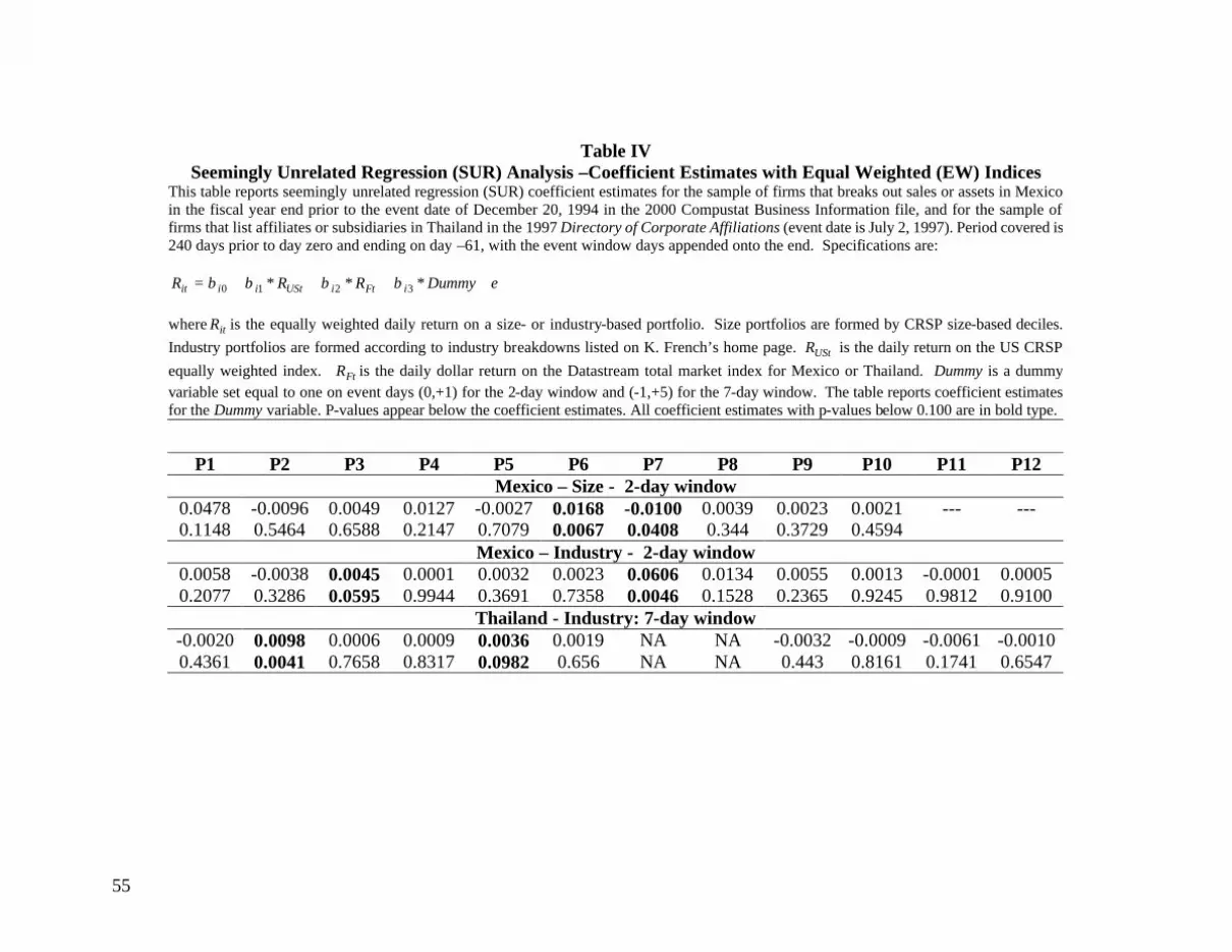
Table IV Seemingly Unrelated Regression (SUR) Analysis –Coefficient Estimates with Equal Weighted (EW) Indices

This table reports seemingly unrelated regression (SUR) coefficient estimates for the sample of firms that breaks out sales or assets in Mexico in the fiscal year end prior to the event date of December 20, 1994 in the 2000 Compustat Business Information file, and for the sample of firms that list affiliates or subsidiaries in Thailand in the 1997 Directory of Corporate Affiliations (event date is July 2, 1997). Period covered is 240 days prior to day zero and ending on day –61, with the event window days appended onto the end. Specifications are:

εββββ ++++= DummyRRR iFtiUStiiit *** 3210 where itR is the equally weighted daily return on a size- or industry-based portfolio. Size portfolios are formed by CRSP size-based deciles. Industry portfolios are formed according to industry breakdowns listed on K. French’s home page. UStR is the daily return on the US CRSP equally weighted index. FtR is the daily dollar return on the Datastream total market index for Mexico or Thailand. Dummy is a dummy variable set equal to one on event days (0,+1) for the 2-day window and (-1,+5) for the 7-day window. The table reports coefficient estimates for the Dummy variable. P-values appear below the coefficient estimates. All coefficient estimates with p-values below 0.100 are in bold type.

P1 P2 P3 P4 P5 P6 P7 P8 P9 P10 P11 P12 Mexico – Size - 2-day window

0.0478 -0.0096 0.0049 0.0127 -0.0027 0.0168 -0.0100 0.0039 0.0023 0.0021 --- --- 0.1148 0.5464 0.6588 0.2147 0.7079 0.0067 0.0408 0.344 0.3729 0.4594

Mexico – Industry - 2-day window 0.0058 -0.0038 0.0045 0.0001 0.0032 0.0023 0.0606 0.0134 0.0055 0.0013 -0.0001 0.0005 0.2077 0.3286 0.0595 0.9944 0.3691 0.7358 0.0046 0.1528 0.2365 0.9245 0.9812 0.9100

Thailand - Industry: 7-day window -0.0020 0.0098 0.0006 0.0009 0.0036 0.0019 NA NA -0.0032 -0.0009 -0.0061 -0.0010 0.4361 0.0041 0.7658 0.8317 0.0982 0.656 NA NA 0.443 0.8161 0.1741 0.6547

56

Table V Individual Firm Results from SUR Regressions

This table reports results from SUR regressions of individual firm time series. Firms are those that break out sales or assets in Mexico in the fiscal year end prior to the event date of December 20, 1994 in the 2000 Compustat Business Information file, and those that list affiliates or subsidiaries in Thailand in the 1997 Directory of Corporate Affiliations (event date is July 2, 1997). The regression specification is:

εββββ ++++= DummyRRR FtUStit *** 3210 Where itR is the firm’s daily return, UStR is the daily return on the US CRSP equally weighted index (EW). FtR is the daily return on the Datastream total market index for Mexico or Thailand. Dummy is a dummy variable set equal to one on event days (0,+1) for the 2-day window and (-1,+5) for the 7-day window. Specification is estimated over event days –241 to –61, with the event window days appended onto the end of the series. The table reports the percentage of times that the Dummy coefficient estimates are significantly different from zero in a two-sided test at the 5 percent level. Mexico Thailand 2-day 7-day 2-day 7-day Positive tail 8.09% 4.02% 11.27% 2.82% Negative tail 4.04% 2.02% 1.41% 2.82%

57

Table VI Individual Firm Volatility Results from SUR Regressions

This table reports results from SUR regressions of individual firm time series. Firms are those that break out sales or assets in Mexico in the fiscal year end prior to the event date of December 20, 1994 in the 2000 Compustat Business Information file, and those that list affiliates or subsidiaries in Thailand in the 1997 Directory of Corporate Affiliations (event date is July 2, 1997). The regression specification is:

2 2 20 1 2 3it USt FtR * R * R * Dummy= β + β + β + β + ε

Where itR is the firm’s daily return, UStR is the daily return on the US CRSP equally weighted index (EW). FtR is the daily return on the Datastream total market index for Mexico or Thailand. Dummy is a dummy variable set equal to one on event days (0,+1) for the 2-day window and (-1,+5) for the 7-day window. Specification is estimated over event days –241 to –61, with the event window days appended onto the end of the series. The table reports the percentage of times that the Dummy coefficient estimates are significantly different from zero in a two-sided test at the 5 percent level.

Mexico Thailand 2-day 7-day 2-day 7-day Positive tail 11.42% 12.06% 8.45% 9.86% Negative tail 5.41% 3.40% 4.23% 0.00%

58

Table VII Summary Statistics for Abnormal Return Measures

This table provides summary descriptive statistics for abnormal return measures for the sample of firms that breaks out sales or assets in Mexico in the fiscal year end prior to the event date of December 20, 1994 in the 2000 Compustat Business Information file, and for the sample of firms that list affiliates or subsidiaries in Thailand in the 1997 Directory of Corporate Affiliations (event date is July 2, 1997). Abnormal returns are calculated with daily data for a 2-day event window (0,+1) and a 7-day event window (-1,+5). Cumulative abnormal returns (CAR) are calculated with a market model, using the CRSP equally weighted index (EW), and a foreign market index stated in US dollar terms (Datastream’s total market index for Mexico or Thailand). Mex and Th are the dollar returns on the Mexican and Thai stock indices, respectively.

2-day 7-day Index N Mean Median Std Dev Skewness Kurtosis Index N Mean Median Std Dev Skewness Kurtosis Mexico CAR 297 0.0065 0.0015 0.0500 2.1301 15.4839 CAR 297 0.0202 0.0146 0.0703 0.0265 5.8088 Mex 2 -0.0698 -0.0698 0.0411 0.0000 1.0000 Mex 7 -0.0398 -0.0407 0.0853 0.4641 1.9050 Thailand CAR 71 0.008 0.009 0.026 1.063 6.188 CAR 71 0.005 0.002 0.048 -0.221 3.002 Thai 2 0.0504 0.0504 0.1275 0.0000 1.0000 Thai 7 -0.0087 -0.0348 0.0843 0.5923 2.4744

59

Table VIII Summary Statistics for Abnormal Returns:

Splitting the Sample into Positive and Negative Return Sub-Samples This table provides summary descriptive statistics for abnormal return measures for the sample of firms that breaks out sales or assets in Mexico in the fiscal year end prior to the event date of December 20, 1994 in the 2000 Compustat Business Information file, and for the sample of firms that list affiliates or subsidiaries in Thailand in the 1997 Directory of Corporate Affiliations (event date is July 2, 1997). Abnormal returns are calculated with daily data for a 2-day event window (0,+1) and a 7-day event window (-1,+5). Cumulative abnormal returns (CAR) are calculated with a market model. Market returns are measured with the CRSP equally weighted index (EW), and are adjusted with both the US index and a foreign market index stated in US dollar terms (Datastream’s total market index for Mexico or Thailand). The table reports the means and medians for sub-samples of the firms separated into those with positive or negative abnormal returns.

Mexico Positive Return Firms Negative Return Firms N Mean Median N Mean Median 2-day window 151 0.0372 0.0249 146 -0.0254 -0.0178 7-day window 185 0.0588 0.0447 112 -0.0435 -0.0298

Thailand

Positive Return Firms Negative Return Firms N Mean Median N Mean Median 2-day window 46 0.0216 0.0166 25 -0.0167 -0.0139 7-day window 37 0.0406 0.0329 34 -0.0335 -0.0201

60

Table IX Estimates of Revisions to the Value of Mexican Cash Flows

The table reports estimates of the revisions to the value of Mexican cash flows based on changes in total firm value. The sample includes firms that break out sales or assets in Mexico alone (ie, not combined with any other region) for the fiscal year end prior to the event date of December 20, 1994 in the 2000 Standard and Poor’s Compustat Business Information file. Comparable data for Thailand are unavailable. Estimates are based on the equation:

Estimate of revision = ashFlowsTotalFirmCMexican

CAR/

Where CAR is the cumulative abnormal return calculated over a 2-day window (0,+1) or a 7-day window (-1, +5), from a market model with the CRSP equally weighted market index. Mexican/Total Firm Cash Flows are proxied with the ratio of Mexican/Total Firm assets or sales as of the fiscal year end prior to the event.

Proxy for Revision to Cash Flows Window Exposure Cash Flows N Max Min Mean Median

2-day + Assets 11 12.418 0.070 2.749 0.477

+ Sales 10 18.886 0.047 3.728 0.179 - Assets 13 -0.018 -0.855 -0.303 -0.255 - Sales 12 -0.008 -4.282 -0.871 -0.328

7-day + Assets 15 35.638 0.183 5.173 0.880 + Sales 13 16.288 0.150 3.381 0.829 - Assets 9 -0.070 -1.344 -0.426 -0.170 - Sales 9 -0.070 -12.871 -2.197 -0.597