Evolution of topology in axi-symmetric and 3-d

viscous flows

G. Scheuermann 1, W. Kollmann 2, X. Tricoche 1 and T. Wischgoll 1

1Department of Computer Science, University of Kaiserslautern

D-67653 Kaiserslautern, Germany2 MAE Dept, University of California Davis

Davis, CA 95616, USA

Contact e-mail:scheuer,tricoche,wischgol@informatik.uni-kl.de, wkollmann@ucdavis.edu

Abstract

Topological methods are used to establish global and to extract local structure properties

of vector fields in axi-symmetric and 3-d flows as function of time. The notion of topological

skeleton is applied to the interpretation of vector fields generated numerically by the Navier-

Stokes equations. The flows considered are swirling jets with super-critical swirl numbers that

show low Reynolds number turbulence in the break-up region.

1 Introduction

A numerical study is conducted to investigate the temporal development of flow structures con-nected with the vortex breakdown in swirling free jets. There is experimental evidence (see Billantet al. [1]) that swirling jets exhibit a rich variety of flow phenomena. Simplified model equationsassuming steady and rotationally symmetric motion above a conical stream surface show bi- andmulti-stability (see [3], [4], [5], [6]) of several flow forms such as hysteresis and negative thrustphenomena. Direct numerical simulations at moderate Reynolds numbers allow relaxation of themodel restrictions. The results show the development of the conical jet layer and its break upinto three-dimensional vortex structures for moderate Reynolds numbers. The detection of thesestructures requires sophisticated tools, that are applicable to two and three dimensional, steadyand unsteady flows. It is essential for the interpretation of these fields to reduce their propertiesto the bare minimum, hence the notion of the topological skeleton, introduced by Fomenko (see[7], [8]) for the classification of integrable Hamiltonian systems, is applied to the present case. Thepaper presents the theoretical aspects of vector field topology and numerical methods for theircomputation. The emphasis is on vector lines in 2-d sections of axi-symmetric and 3-d flows.

The organisation of the paper is as follows. First, the numerical method for the solution of theincompressible Navier-Stokes equations is briefly outlined. Then basic definitions and theorems forthe topology of steady vector fields are discussed followed by the consideration of the topologicalskeleton and its temporal evolution. Numerical methods for the computation of the evolution ofthe vector field topology are developed and results for the swirling jet flows are presented.

2 Navier-Stokes solver

A hybrid spectral finite-difference method (developed in [9]) is used to solve the Navier-Stokesequations in cylindrical coordinates. The method will be outlined briefly, the details including theverification of its accuracy and convergence properties are available in [9] and [10]. The methodtakes advantage of the fact that all dependent variables ϕ are periodic with respect to azimuthalvariable θ, hence is the discrete Fourier transform FN (Fourier collocation method, Canuto etal.,[11]) applicable

ϕ(k) = FN (ϕ) ≡1

N

N−1∑

j=0

ϕ(θj) exp(−ikθj), k = −N/2, · · · , N/2 − 1

2

ϕ(θj) = F−1N (ϕ) ≡

N/2−1∑

k=−N/2

ϕ(k) exp(ikθj), j = 0, · · · , N − 1 (1)

where F−1N denotes the inverse transform and the θj = 2πj/N are the discrete collocation points.

The dependent variables (see [9]) in the present formulation are the complex-valued Fouriermodes (k denotes the discrete azimuthal wavenumber) of:

The azimuthal velocity modes vθ(r, k, z, t) for 0 ≤ k ≤ N2

,

the azimuthal vorticity modes Ωθ(r, k, z, t) for 0 ≤ k ≤ N2

,

the streamfunction modes Ψ(r, k, z, t) for 0 ≤ k ≤ N2

,

the pressure modes p(r, k, z, t) for 1 ≤ k ≤ N2

.The azimuthal momentum balance provides the equation for the velocity modes vθ(r, k, z, t)

∂vθ

∂t(k) + FN [vr

∂vθ

∂r+ vz

∂vθ

∂z+

vθ

r(∂vθ

∂θ+ vr)] = −i

k

rρp(k)

+1

Re[∂

∂r(1

r

∂

∂r(rvθ(k))) −

k2

r2vθ(k) +

∂2vθ

∂z2(k) + 2i

k

r2vr(k)] (2)

where the convective terms are evaluated using FFT, Re denotes the Reynolds number. Applicationof the divergence operation to the momentum balances produces the equations for the pressuremodes p(r, k, z, t), which emerge in the form

1

r

∂

∂r(r

∂p

∂r) −

k2

r2p +

∂2p

∂z2=

−ρFN [(∂vr

∂r)2 +

1

r2(∂vθ

∂θ+ vr)

2 + (∂vz

∂z)2 +

2

r

∂vθ

∂r(∂vr

∂θ− vθ) + 2

∂vr

∂z

∂vz

∂r+

2

r

∂vz

∂θ

∂vθ

∂z] (3)

The transport equation for the azimuthal vorticity component Ωθ follows from its definition andthe momentum balances. It appears in the form

∂Ωθ

∂t=

∂

∂r[FN (vθΩr) −FN(vrΩθ)] +

∂

∂z[FN (vθΩz) −FN(vzΩθ)]

+1

Re[∂

∂r(1

r

∂

∂r(rΩθ(k))) −

k2

r2Ωθ(k) +

∂2Ωθ

∂z2(k) + 2i

k

r2Ωr(k)] (4)

It is shown in [9] that a complex-valued streamfunction Ψ(r, k, z, t) exists for each wavenumber kas a consequence of the Fourier transformed mass balance, which can be recast as the divergenceof a 2-d vector being zero. This results in Poisson-Helmholtz type equations for Ψ(r, k, z, t)

∂

∂r

(

1

r

∂

∂r(rΨ)

)

+∂2Ψ

∂z2= Ωθ + ik

∂〈vθ〉

∂z(5)

The velocity components can be recovered from

−rvz =∂

∂r(rΨ), vr =

∂Ψ

∂z− ik〈vθ〉 (6)

once vθ and the streamfunctions Ψ have been computed. The angular brackets are essential forthe streamfunction formalism (5), (6), they are defined by

〈Φ〉(r, k, z, t) ≡1

r

r∫

0

dr′Φ(r′, k, z, t) (7)

The presence of singular coefficients in (2) to (5) requires careful analysis of the pdes for r → 0([12], [13]). The results (details in [9]) can be summarized as follows:

(I) Scalar modes Φ(r, k, z, t) and axial vector components satisfy O(Φ(r, k, z, t)) = rk and aresymmetric with respect to r for k even and skew-symmetric for k odd.

3

(II) Radial and azimuthal vector components satisfy the kinematic conditions vr(0, k, z, t) +ikvθ(0, k, z, t) = 0 and both modes are symmetric with respect to r for k = 1, and O(vr(r, k, z, t)) =O(vθ(r, k, z, t)) = r for k = 0 and O(vr(r, k, z, t)) = O(vθ(r, k, z, t)) = rk−1 for k > 1, and theyare skew-symmetric with respect to r for k even and symmetric for k odd. The complex-valuedstreamfunctions can be shown to obey O(Ψ(k)) = rk+1 and are skew-symmetric with respect to rfor k even, symmetric for k odd.

The conditions at the axis and the entrance, exit and outer boundaries are either Dirichletor Neumann type or a combination of Dirichlet and Neumann conditions. Specifically, the axisconditions cannot be chosen arbitrarily but follow from the symmetry and smoothness properties atr = 0; the Fourier modes satisfy either homogenous Dirichlet or homogeneous Neumann conditions.At entrance and outer boundaries Dirichlet conditions are prescribed and convective boundaryconditions are used at the exit.

The sectional domain (r, z) ∈ [0, R] × [0, Lz] is rectangular, it may be semi-infinite (R = ∞).It is mapped onto the unit quadrangle using separable and analytic functions. It is discretizedwith respect to radial and axial directions with uniform spacing in the image domain [0, 1]× [0, 1].Either central differences are used for first and second derivatives with explicit filters (Kennedy &Carpenter [14]) applied to the increments of the transport equations or upwind-biased differences(Li[15]) for the convective terms and central differences for the non-convective terms. The filterorder is chosen such that it does not degrade the accuracy of the finite-difference schemes, no filtersare applied for the upwind-biased schemes. The numerical integration required in (7) is done usinga fourth order accurate difference method.

The time integrator is an explicit 4th-order state space Runge-Kutta method that requiresminimal storage (see [9]). The Poisson/Helmholtz equations (2) and (5) are solved using LU-decomposition (LINPACK, see Dongarra et al.[16]) combined with deferred corrections to reducethe bandwidth of the coefficient matrix.

3 Topology of Steady Vector Fields

The study of the topology requires clear definitions and numerical methods for their computation.We define in the following the basic notions of vector field topology relevant for the present pur-pose. The description is similar to Fomenko et al. [7], [8], but the results in our examples arefundamentally different since our fields do not allow a Hamiltonian function. We start with somesimple terms.

First, we clarify two definitions widely used in fluid mechanics: Streamlines and pathlines.Given an unsteady vector field v(x, t) we compute the streamlines Φ(t∗) as solutions of the initialvalue problem

dΦ

dt∗= v(Φ(t∗), t) (8)

with initial conditions determining the desired streamline. Streamlines are computed for the fixedtime t (instantaneous integral curves or snapshots) and the picture generated by them changeswith time if the vector field is unsteady. On the other hand are the pathlines the solutions of

dΦ

dt= v(Φ(t), t) (9)

plus initial conditions and it follows that pathlines are different from streamlines if the vector fieldis unsteady. The pathlines are the vector lines in the mathematical literature. We consider inthe present chapter steady vector fields and instant snapshots of unsteady fields in the followingsection. The vector lines are streamlines and the line parameter t is time if the field is steady, butfor unsteady fields it is isomorphic to arclength.

Definition 3.1 A planar vector field is a map

v : D → R2 , (10)

x 7→ v(x) .

4

Definition 3.2 An integral curve through a point x ∈ R2 of a vector field v : D → R

2 is amap

αx : R ⊃ I → D , (11)

where

αx(0) = x0 , (12)

αx(t) = v (α(t)) , ∀ t ∈ I . (13)

Concerning the theorem on existence and uniqueness of integral curves, the Lipschitz condition

has to be satisfied:

Definition 3.3 Let U ⊂ R2 be an open subset. A continous vector field v : R

2 → R2 satisfies a

Lipschitz condition on U provided there exists a real number K > 0 such that

‖Dv(x) − Dv(y)‖ ≤ K‖x− y‖ (14)

holds for all x, y ∈ U and all t ∈ J where Dv denotes the differential of the vector field v. Theconstant K is called Lipschitz constant.

This allows to formulate the existence and uniqueness theorem:

Theorem 3.4 (Existence and uniqueness of integral curves) Let v : D → R2 be a vector

field satisfying the Lipschitz condition on any open neighborhood around point x ∈ R2. Then there

exists one and only one integral curve through any x0 ∈ R2.

Proof: See [20, pp. 66–68].

We also need some terms for the different directions of the vector field at the boundary.

Definition 3.5 Let D ⊂ R2 be a compact domain of a Lipschitz-continous vector field v : D → R

2.Let d ∈ ∂D be a point on the boundary. We define the following three entities:

(1) The point d is called an outflow point if every integral curve through d ends at d and thereexists an integral curve through d that does not contain another point of ∂D. The set of alloutflow points is called outflow set.

(2) The point d is called a inflow point if every integral curve through d starts at d and thereexists an integral curve through d that does not contain another point of ∂D. The set of allinflow points is called inflow set.

(3) The point d is called a boundary flow point if there exists an integral curve αd : (−ǫ, ǫ) →D, ǫ > 0, through d lying completely inside ∂D. The set of all boundary flow points is calledboundary flow set.

(4) The point d is called boundary saddle (switch point), if it does not belong to the other threetypes.

If a vector field satisfies the Lipschitz condition for an open neighborhood of every point, integralcurves can be extended over the whole time line if they do not reach the boundary at an outflowpoint.

Lemma 3.6 Let v : D → R2 be Lipschitz continuous around each point. Then an integral curve

can be defined up to +∞ if it does not end at an outflow point. It can also be defined from −∞ ifit does not start at an inflow point.

Since we want to keep the following notations simple, we define an integral curve at an inflowpoint as that point for the whole time before it enters the domain. Further, at an outflow point,we extend an integral curve by this point for all the time after it has left the domain. In thisway, all integral curves are defined for all t ∈ R. Topology is really concerned with the asymptoticbehavior of integral curves, so we look at their asymptotic begin and end.

5

BBBBBBBBBBBBBBBBBBBBBBBBBBBBBBBBBBBBBBBBBBBBBBBBBBBBBBBBBBBBBBBBBBBBBBBBBBBBBBBBBBBBBBBBBBBBBBBBBBBBBBBBBBBBBBBBBBBBBBBBBBBBBBBBBBBBBBBBBBBBBBBBBBBBBBBBBBBBBBBBBBBBBBBBBBBBBBBBBBBBBBBBBBBBBBBBBBBBBBBBBBBBBBBBBBBBBBBBBBBBBBBBBBBBBBBBBBBBBBBBBBBBBBBBBBBBBBBBBBBBBBBBBBBBBBBBBBBBBBBBBBBBBBBBBBBBBBBBBBB

BBBBBBBBBBBBBBBBBBBBBBBBBBBBBBBBBBBBBBBBBBBBBBBBBBBBBBBBBBBBBBBBBBBBBBBBBBBBBBBBBBBBBBBBBBBBBBBBBBBBBBBBBBBBBBBBBBBBBBBBBBBBBBBBBBBBBBBBBBBBBBBBBBBBBBBBBBBBBBBBBBBBBBBBBBBBBBBBBBBBBBBBBBBBBBBBBBBBBBBBBBBBBBBBBBBBBBBBBBBBBBBBBBBBBBBBBBBBBBBBBBBBBBBBBBBBBBBBBBBBBBBBBBBBBBBBBBBBBBBBBBBBBBBBBBBBBBBBBBBBBBBBBBBBBBBBBBBBBBBBBBBBBBBBBBBBBBBBBBBBBBBBBBBBBBBBBBBBBBBBBBBBBBBBBBBBBBBBBB

Figure 1: Around a source, every integral curve starts at the source; around a sink, every integralcurve ends at the sink.

Definition 3.7 Let v : D → R2 be a Lipschitz-continous vector field and c : R → R

2 an integralcurve. The set

a ∈ R2|∃(tn)∞n=0 ⊂ R, tn → ∞, lim

n→∞

c(tn) → a (15)

is called ω-limit set of c. The set

a ∈ R2|∃(tn)∞n=0 ⊂ R, tn → −∞, lim

n→∞

c(tn) → a (16)

is called α-limit set of c.

The most common types of limit sets are critical points.

Definition 3.8 A critical point of v : D → R2 is a point p ∈ D with v(p) = 0.

Two cases are of interest: (1) sinks and (2) sources.

Definition 3.9 Let v : D → R2 be a Lipschitz-continous vector field, z ∈ D a critical point. If

there is a neighborhood U ⊂ D of z such that all integral curves in U have a α-limit set consistingonly of z, then z is called a source. If there is a neighborhood U ∈ D of z such that all integralcurves in U have a ω-limit set consisting only of z, then z is called a sink. If there is a neighborhoodU ∈ D of z such that there is a finite number of integral curves that start or end at z and all otherintegral curves leave U in both directions of time, z is called a saddle.

Figure 1 shows a source in the upper part. All integral curves around the critical point startat this critical point. In the lower part, a sink is shown. Every integral curve in the neighborhoodends at the sink. Another type of limit sets are closed integral curves (cycles).

Definition 3.10 Let v : D → R2 be a Lipschitz continuous vector field. A closed streamline

c : R → D of v is a streamline with a t0 ∈ R with

c(t + nt0) = c(t)∀n ∈ N . (17)

(It is assumed that c does not stay at one point all the time, i.e. c(t) is not a critical point.)

.Figure 2 shows a typical example. Such a cycle is called structurally stable if, after small

changes, the vector field still contains a closed streamline. Such stability arguments allow toconcentrate on critical points, boundary regions and closed cycles as possible α- and ω-limit sets

6

Figure 2: A limit cycle may attract streamlines in its neighborhood.

[18],[19]. For our analysis of a vector field, we have to determine the asymptotic behavior of all itsintegral curves. This is done by analyzing the union of all integral curves starting or ending at thesame critical point, same cycle, or the same inflow/outflow region.

Definition 3.11 Let v : D → R2 be a Lipschitz-continous vector field and M ⊂ D. The union

of all integral curves of v that converge to M for t → −∞ is called α-basin of M , denoted byBα(M). The union of all integral curves of v that converge to M for t → ∞ is called ω-basin ofA, denoted by Bω(M).

For sinks and sources, one can prove the following lemma:

Lemma 3.12 Let a be a critical point of a Lipschitz continuous vector field v : D → R2. If a is a

source then Bα(a) is an open subset of D. If a is a sink then Bω(a) is an open subset of D.

Proof: See [19, pp. 181-182].

A similar result holds for cycles, i.e. a structurally stable cycle in 2D can be either a source andits α-basin is an open subset of the domain or it is a sink and its ω-basin is an open subset. Ashort comment on dimension prepares us for the final theorem of the section.

Definition 3.13 If a subset M ⊂ R2 allows a description as a pure n-dimensional manifold, we

define the dimension of M as n.

Remark 3.14 We need the term dimension only for basins. The previous definition means that anopen basin in D is a 2-manifold, a basin consisting of a finite number of streamlines is a 1-manifoldand a basin consisting of a finite number of points is a 0-manifold.

Since we assume that we have only structurally stable limit sets, we obtain a decomposition ofthe domain into disjunct α-basins and a decomposition into disjunct ω-basins if we regard theconnected component of the inflow set and the outflow set also as limit sets.

Theorem 3.15 Let v : D → R2 be a Lipschitz continuous vector field with only structurally stable

limit sets Li ⊂ D, i ∈ I. Let Ai ⊂ D denote the α-basins of the limit sets and Ωi ⊂ D denote theω-basins. Then:

D =⋃

i∈I Ai (18)

D =⋃

i∈I Ωi (19)

As topology of the vector field we define the set of limit sets Li and the connected components ofthe intersections Tij = Ai ∩ Ωj.

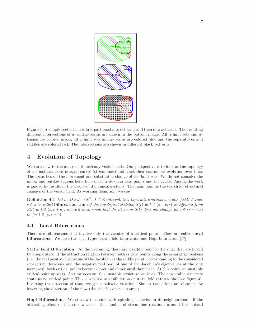
Figure 3 shows the decomposition of a simple academic example flow into α-basins, ω-basins,and their intersections. Since the basins of sources, sinks, cycles, inflow, and outflow regions areall open subsets, the topology can be described by the one-dimensional basin intersections thatform the boundaries of the open basin intersections. Because they separate the open basins, theyare called separatrices. Since the boundary of an open set does not belong to the open set, theseparatrices must start or end at saddles or boundary saddles. This fact is used to calculate thetopology, i.e. we compute only the separatrices and obtain the other basin intersections as theresulting faces in the domain. All limit sets form the topological skeleton Sv together with theseparatrices.

7

00000000000000000000000000000000000000000000000000000000000000000000000000000000

999999999999999999999999999999999999999999999999999999999999999999999999999999999999999999999999999999999999999999999999999999999999999999999999999999999999999999999999999999999999999999999999999999999999999999999999999999999999999999999999999999999999

999999

99999999999999999999999999999999999999999999999999999999999999999999999999999999

999999999999999999999999999999999999999999999999999999999999999999999999999999999999999999999999999999999999999999999999999999999999999999999999999999999999999999

999999

999999999999999999999999999999999999999999999999999999999999999999999999999999999999999999999999999999999999999999999999999999999999999999999999999999999999999999999999999999999999999999999999999999

AAAAAAAAAAAAAAAAAAAAAAAAAAAAAAAAAAAAAAAAAAAAAAAAAAAAAAAAAAAAAAAAAAAAAAAAAAAAAAAAAAAAAAAAAAAAAAAAAAAAAAAAAAAAAAAAAAAAAAAAAAAAAA

CCCCCCCCCCCCCCCCCCCCCCCCCCCCCCCCCCCCCCCCCCCCCCCCCCCCCCCCCCCCCCCCCCCCCCCCCCCCCCCC

BBBBBBBBBBBBBBBBBBBBBBBBBBBBBBBBBBBBBBBBBBBBBBBBBBBBBBBBBBBBBBBBBBBBBBBBBBBBBBBBBBBBBBBBBBBBBBBBBBBBBBBBBBBBBBBBBBBBBBBBBBBBBBBBBBBBBBBBBBBBBBBBBBBBBBBBBBBBBBBBBB

Figure 3: A simple vector field is first partioned into α-basins and then into ω-basins. The resultingdifferent intersections of α- and ω-basins are shown in the bottom image. All α-limit sets and α-basins are colored green, all ω-limit sets and ω-basins are colored blue and the separatrices andsaddles are colored red. The intersections are shown in different black patterns.

4 Evolution of Topology

We turn now to the analysis of unsteady vector fields. Our perspective is to look at the topologyof the instantaneous integral curves (streamlines) and track their continuous evolution over time.The focus lies on the movement and substantial change of the limit sets. We do not consider theinflow and outflow regions here, but concentrate on critical points and the cycles. Again, the workis guided by results in the theory of dynamical systems. The main point is the search for structuralchanges of the vector field. As working definition, we use

Definition 4.1 Let v : D×J → R2, J ⊂ R interval, be a Lipschitz continuous vector field. A time

s ∈ J is called bifurcation time if the topological skeleton S(t) at t ∈ (s − δ, s) is different fromS(t) at t ∈ (s, s + δ), where δ is so small that the Skeleton S(t) does not change for t ∈ (s − δ, s)or for t ∈ (s, s + δ).

4.1 Local Bifurcations

There are bifurcations that involve only the vicinity of a critical point. They are called localbifurcations. We have two such types: static fold bifurcation and Hopf bifurcation [17].

Static Fold Bifurcation At the beginning, there are a saddle point and a sink, that are linkedby a separatrix. If the attraction relation between both critical points along the separatrix weakens(i.e. the real positive eigenvalue of the Jacobian at the saddle point, corresponding to the consideredseparatrix, decreases and the negative real part of one of the Jacobian’s eigenvalues at the sinkincreases), both critical points become closer and closer until they meet. At this point, an unstablecritical point appears. As time goes on, this unstable structure vanishes: The new stable structurecontains no critical point: This is a pairwise annihilation or static fold catastrophe (see figure 4).Inverting the direction of time, we get a pairwise creation. Similar transitions are obtained byinverting the direction of the flow (the sink becomes a source).

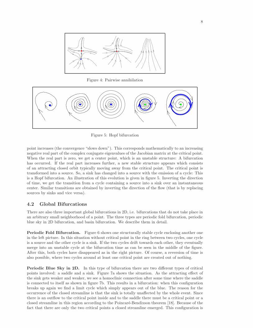
Hopf Bifurcation. We start with a sink with spiraling behavior in its neighborhood. If theattracting effect of this sink weakens, the number of streamline rotations around this critical

8

Figure 4: Pairwise annihilation

Figure 5: Hopf bifurcation

point increases (the convergence “slows down”). This corresponds mathematically to an increasingnegative real part of the complex conjugate eigenvalues of the Jacobian matrix at the critical point.When the real part is zero, we get a center point, which is an unstable structure: A bifurcationhas occurred. If the real part increases further, a new stable structure appears which consistsof an attracting closed orbit typically moving away from the critical point. The critical point istransformed into a source. So, a sink has changed into a source with the emission of a cycle: Thisis a Hopf bifurcation. An illustration of this evolution is given in figure 5. Inverting the directionof time, we get the transition from a cycle containing a source into a sink over an instantaneouscenter. Similar transitions are obtained by inverting the direction of the flow (that is by replacingsources by sinks and vice versa).

4.2 Global Bifurcations

There are also three important global bifurcations in 2D, i.e. bifurcations that do not take place inan arbitrary small neighborhood of a point. The three types are periodic fold bifurcation, periodicblue sky in 2D bifurcation, and basin bifurcation. We describe them in detail.

Periodic Fold Bifurcation. Figure 6 shows one structurally stable cycle enclosing another onein the left picture. In this situation without critical point in the ring between two cycles, one cycleis a source and the other cycle is a sink. If the two cycles drift towards each other, they eventuallymerge into an unstable cycle at the bifurcation time as can be seen in the middle of the figure.After this, both cycles have disappeared as in the right picture. Of course, a reversion of time isalso possible, where two cycles around at least one critical point are created out of nothing.

Periodic Blue Sky in 2D. In this type of bifurcation there are two different types of criticalpoints involved: a saddle and a sink. Figure 7a shows the situation. As the attracting effect ofthe sink gets weaker and weaker, we see a homoclinic connection after some time where the saddleis connected to itself as shown in figure 7b. This results in a bifurcation: when this configurationbreaks up again we find a limit cycle which simply appears out of the blue. The reason for theoccurrence of the closed streamline is that the sink is totally unaffected by the whole event. Sincethere is an outflow to the critical point inside and to the saddle there must be a critical point or aclosed streamline in this region according to the Poincare-Bendixson theorem [18]. Because of thefact that there are only the two critical points a closed streamline emerged. This configuration is

9

Figure 6: Periodic fold bifurcation

a)b)

c)

Figure 7: Periodic Blue Sky in 2D

shown in figure 7c. Other bifurcations of the same type can be constructed by replacing the sinkwith a source or by inverting the direction of time.

Basin Bifurcation The remaining bifurcation that plays a role in our analysis does not involvecritical points or cycles but only separatrices. It is called basin bifurcation, since only the basins andtherefore the connectivity of the limit sets changes. It is characterized by a heteroclinic connectionbetween two saddles at the bifurcation time. Figure 8 shows this event. The separatrices startingat the two saddles come closer and closer until they coincide at the bifurcation time. After this,the connection between the limit sets has changed — we have other basins than before.The evolution of topology can now be defined.

Definition 4.2 Let v : D×J → R2, J = [s0, s1] ⊂ R an interval, be a Lipschitz continuous vector

field. Let the vector field vt : D → R2, vt(x) = v(x, t) contain only structurally stable limit sets for

all t ∈ J except at a finite number of bifurcation times t1, . . . , ti, . . . , tm ∈ J . The evolution oftopology of v is the topology at s0, the maps of the movement of all limit sets, the maps of themovement of the separatrices, and the type and location of all bifurcations.

We assume that our unsteady vector field is structurally stable, so that there takes place onlyone bifurcation at a bifurcation time. Especially, we do not consider combinations of bifurcationsthat interfer with each other. The evolution can be described by the movement of the limit sets,the movement of the separatrices and the bifurcations. The information about the bifurcationsincludes type, time, location, and the involved limit sets as well as separtrices.

5 Computation of Topology

For the topology, we need the limit sets and the basin boundaries as defined in section 3. Sincewe leave the boundary regions aside (for a clear analysis, see [22]), we are left with critical points,cycles, and the separatrices originating at saddles.

10

Figure 8: Basin bifurcation

Saddle Point:R1<0, R2>0,I1 = I2 = 0

Repelling Focus: R1 = R2 >0, I1 = -I2 <> 0

Attracting Focus:

I1 = -I2 <> 0R1 = R2 < 0,

Repelling Node:

I1 = I2 = 0R1, R2 > 0,

Attracting Node: R1, R2 < 0, I1 = I2 = 0

Figure 9: Common types of critical points.

5.1 Critical Points

A critical point is a zero of the field, so we have to do a zero search. This task depends heavilyon the used interpolation scheme. In our case, we obtain a cartesian grid in a plane cut alongthe rotation axis of the cyclindric domain from the numerical method. Since we want to keep thecomputation effort, especially in the next section, at a manageable level, we triangulate the gridand use linear interpolation in each triangle. For the critical points, we can now solve a simplelinear equation in each triangle. If the resulting zero is in the triangle, we have a critical point. Itstype is easily found by calculating the (complex) eigenvalues of the Jacobian:

• Two negative real parts correspond to a sink.

• Two positive real parts correspond to a source.

• Mixed real parts correspond to a saddle.

A zero eigenvalue means a whole critical line of zeros in the triangle which we have excluded byour assumption of structurally stable vector fields. (We have also not found this case in practice.)Figure 9 shows the different cases. An analysis of critical points at the vertices of the grid is alittle bit more difficult, but it can be done, see [23].

5.2 Closed Streamlines

As mentioned before, a closed streamline d : R → R2, t 7→ d(t) is a streamline of a vector field

v such that there is a t0 ∈ R/0 with d(t + nt0) = d(t)∀n ∈ N and d not constant. In this

11

subsection we present an algorithm that detects whether an arbitrary streamline c converges tosuch a closed curve. This means that c has d as α- or ω-limit set depending on the orientationof integration. We do not assume any knowledge on the existence or location of the closed curve,so that the algorithm can detect closed streamlines. The principle of the algorithm works on anypiecewise defined planar vector field where one can determine the topology inside the pieces. Thebasic idea of the algorithm is to determine a region of the vector field that is never left by astreamline. In case of a continuous vector field the Poincare-Bendixson-Theorem ensures that thisstreamline approaches a closed streamline if no critical point exists in that region. A streamlineapproaching a closed streamline has to reenter the same cell. In this case we check if the cells werecrossed by the streamline in the same order for the last two turns. This results in a cell cycle whichidentifies the above mentioned region. To examine if this cell cycle is left by the streamline wedetect possible changes by checking the edges of the cells of the cell cycle. Therefore we identifypoints on each edge which we call potential exits where an outflow out of the cell cycle may occurin the vicinity. These points are identical with the vertices of the edge and points where the vectorfield is tangential to the edge.

exit

Figure 10: If a real exit can be reached, the streamline will leave the cell cycle.

We have to figure out if the actually investigated streamline will leave the cell cycle near suchan exit. Therefore we integrate a streamline backwards from the potential exit to see if it leavesthe cell cycle. If it does not leave after it crossed every cell of the cell cycle it converges to ourstreamline. We call this potential exit a real exit because the streamline will leave the cell cycleafter a finite number of turns near that exit. Figure 10 displays an example for that case.

If the backward integrated streamline leaves the cell cycle, there will also be an entry pointas shown in figure 11. A streamline starting at that point cannot be crossed by our actuallyinvestigated streamline. Consequently we cannot leave the cell cycle at this exit.

exit

exit

entry

Figure 11: If no real exit can be reached, the streamline will approach a closed streamline.

If there is no real exit for the streamline, we have proven that the streamline will never leave

12

the cell cycle. If there is no critical point inside the cell cycle the Poincare-Bendixson-Theoremensures that there exists a closed streamline in our cell cycle and the integral curve tends towardit. The exact position of the closed streamline can be found using the Poincare map.

Let us assume that we have a two-dimensional continuous vector field containing one closedstreamline. Then we can choose a point P on the closed streamline and draw a cross section Swhich is a line segment nowhere parallel to the vector field. This line segment is then called aPoincare section. If we start a streamline at an arbitrary point x on S and follow it until we crossthe Poincare section S again, we get another point R(x) on S. This results in the Poincare mapR. Figure 12 illustrates the situation. The left part shows the Poincare section with the closedstreamline in the middle, drawn with a thicker line. The right part displays the Poincare mapitself.

y

R(y)

x

S

R(x)

x

P

P

R(x)R

S

S

Figure 12: Poincare section and Poincare map.

R maps the point on the closed streamline onto itself because the closed streamline will intersectthe Poincare section always at the same point. Consequently, it is sufficient to find the fix point toget a point on the closed streamline. If we find a cell cycle we can use the edge where we detectedthe cell cycle for the first time as a Poincare section. To find the fix point of the Poincare mapwe do a binary search: first we divide the edge into two parts at the mid point of the edge. Thenwe check which part gets intersected by the streamline starting at the intersection point after oneturn. This part is subdivided again and we start another streamline. This continues until we areclose enough at the fix point of the Poincare map. If we start a streamline at this point we getthe whole closed streamline after we crossed every cell of the cell cycle. This method terminatesbecause we proved in the previous step where we detected the cell cycle that we converge to aclosed streamline.

5.3 Separatrices

In section 3, it was explained that the separatrices can be found at the saddle points. Since wehave only linear saddles in our vector field, we can use the eigenvectors of the Jacobian to findthe separatrices in the triangle containing the saddle, see figure 13. We extend the separatricesby using an adaptive Runge-Kutta-Fehlberg integration [21]. We check for reaching the boundary,running into a critical point, and approaching a cycle as explained above. This completes ournumerical analysis of the topology.

6 Computation of the Evolution

For the calculation of the evolution of the topology, we need an interpolation scheme over time.Since we want to keep the calculations simple, we do a linear interpolation between the stored time

13

Figure 13: Separatrices for linear saddle.

t = t t = t t = t t = ti i+1 i+2 i+3

X

Y

T

t = t i+1t = t i

T

Figure 14: Space/Time grid

steps from the numerical simulation. The resulting grid is shown in figure 14.

Definition 6.1 Let vj : D → R2 be the given vector fields at time steps t0, . . . , ti, . . . , tm. Then

we define

v : D × [t0, tm] → R2 (20)

(x, t) 7→ti+1 − t

ti+1 − tivi(x) +

t − titi+1 − ti

~ai+1vi+1(x), t ∈ [ti, ti+1].

We can now use the results from section 5 to obtain all critical points, cycles, and separatrices att0. We have to find now all the paths of critical points in all the prism cells, connect them andfind the local bifurcations along the way.

6.1 Evolution of Critical Points

We locate and track critical points over time, using the interpolation scheme presented above. Inparticular, we seek the local bifurcations that may modify the topological structure: fold and Hopfbifurcations. To reduce the memory needs of our method, we do not process the whole grid atonce: We consider only two consecutive time planes and handle the prism cells connecting them,forming a “time slice”. More precisely, we first determine for each prism cell the possible entryand exit positions of singular points and then reconnect these pieces of information to track everysingularity from one time plane to the next.

14

Cellwise Analysis. The interpolant has been chosen so that it contains at most one criticalpoint for a fixed value of t in a cell. This is due to the affin linear nature of its restriction to anytime plane. If t moves from ti to ti+1, the singularity position describes a 3D curve. Yet, we areonly interested in the curve sections that intersect the interior domain of the considered prism cell.A simple way to determine them is to consider the singularities lying on the side faces of the prism:Two triangular faces lying in t = ti and t = ti+1 and 3 quadrilaterals connecting them. Finding theposition of a singularity in each prism face requires the solution of a simple linear (resp.quadratic)system. If this is done, we sort the found (3D) positions in ascending time order and associatethem pairwise. Indeed, since only one critical point can be present in a prism cell at a given timet, we know that a critical point must first leave the cell before it reenters it later. So, for each pair,we identify an entry and an exit position. We now need to pay attention to the singularity typesto complete the topological information. The generic types of linear singularities are source, sinkor saddle (omitting center points that correspond to a transition between source and sink). Thetransition from one type to another constitutes a bifurcation. Since a prism cell contains at mostone critical point for a given t, we can assert that no fold bifurcation (involving two critical points)can occur inside it: A fold bifurcation must occur at the cell boundary. Consequently, we onlyseek Hopf bifurcations occurring between two consecutive entry and exit points. Practically, thedetermination of a singularity type is based upon the eigenvalues of the Jacobian at its position.Thus we compute the Jacobian matrix and its associated eigenvalues at each entry and exit pointand check if they are the same. If this is the case, we can assert that no Hopf bifurcation hasoccurred since, otherwise, at least two bifurcations have taken place, which is impossible since ourinterpolant varies linearly over time. If the type has changed, a Hopf bifurcation is on the way.Because a Hopf bifurcation corresponds to a transition from a repelling to an attracting nature,the instantaneous nature of the intermediate singularity is a center and the trace of the Jacobian iszero at this point, which we use as criterion to determine the exact time location of the bifurcation.With the expression above, we obtain:

tr(J(t)) = tr( a11(t) a12(t)

a21(t) a22(t)

)

= a11(t) + a22(t) = 0.

After straightforward calculus, we get finally

t = ti − (ti+1 − ti) ×ai11 + ai

22

ai+111 − ai

11 + ai+122 − ai

22

.

The corresponding position (x(t), y(t), t) is the location of a Hopf bifurcation.

Tracking between the Prisms. At this stage, every cell knows the successive entry and exitpositions of the critical point paths through its interior domain, as well as the possible presence ofa Hopf bifurcation on the way. Yet, this information is scattered and must be reconnected to offera global view of the topology evolution over time. A fundamental aspect of this task is to detectand identify the bifurcations that may take place on the faces. They are detected when connectingcritical point path sections lying in neighbor cells as we show next.

We start in the time plane t = ti. The restriction of the grid to this plane is a triangulation.In a boolean array, we indicate for each triangle if its corresponding prism must be further inspectedor not. If it has to be inspected, we check the information collected during the cell analysis for apath section starting at an entry point located on the considered triangle face. This provides uswith an exit point at which the tracking must be proceeded. This exit point can either lie on aside (quadrilateral) face of the prism or on the triangle face lying in t = ti+1. In the latter case,we signify in the boolean array of the next time plane t = ti+1 that this triangle must be furtherinspected. If the path leaves the cell at t∗ < ti+1 (side face), then it enters a neighboring cell at thesame time. Back to a 2D representation, we get in time plane t = t∗ a critical point lying on thecommon edge of both neighboring triangle cells. Due to the discontinuity of the Jacobian matrixthrough this edge, the critical point may have another type when considered from the other side.This simple argument explains the possible existence of a bifurcation in such cases. Two situationsmay actually occur.

15

SADDLE

SINK

SOURCE

SOURCE

CREATION ANNIHILATION HOPF

time

X,Y

SADDLE

SINK

CELLFACES

Figure 15: Possible cases when leaving a prism cell through a rectangular face

• There is a simple crossing of a critical point from one cell to another cell where no criticalpoint was present so far. In this case, the type may change but, a saddle remains a saddle. Asource may become a sink and vice versa. As mentioned previously, the transition source/sinkor sink/source is a so-called Hopf bifurcation. We easily detect it by checking if the type ofa source (resp. a sink) path changes after passing the face.

• The second situation corresponds to a merging of two coexisting critical points in neighboringcells on their common face (common edge in 2D). Now, an important property of the piecewiseaffin linear interpolant over a triangulation is that two neighboring triangles cannot containtwo critical points with the same type which implies that only a saddle and a source ora saddle and a sink can merge that way. This type of bifurcation has been considered insection 4: It is a static fold bifurcation or its inverse.

When we leave the current cell through a side face, and a possible bifurcation has been detected,we identify this position. We proceed with tracking the path by asking the neighbor cell for thenext exit position. We get three possible answers.

1. The exit position lies in the time plane t = ti+1: We have reached the next time plane.The corresponding triangle face is marked true in the boolean array corresponding to thenext time plane.

2. The “exit” position lies in the time plane t = ti: If we were tracking the current pathforward so far, we have found a pairwise annihilation. In this case, the corresponding triangleis set to false in the boolean array of t = ti, indicating that this cell has been processednow.

3. The exit position lies on a side face for t = t#. If t# < t∗ and we were tracking the currentpath forward so far, we have found a pairwise annihilation and proceed with backwardtracking. If t# > t∗ and we were tracking the current path backward so far, we have found apairwise creation and proceed with forward tracking. In this case, we are back to the currentsituation where one enters a cell through a side face.

The possible cases are illustrated in figure 15.

6.2 Tracking the Cycles

Since there must be a critical point inside each closed streamline we use the critical point pathcontaining a Hopf bifurcation as a starting point for our streamline algorithm from subsection 5.2which detects the closed streamline if it exists. Therefore we follow the critical point path in

16

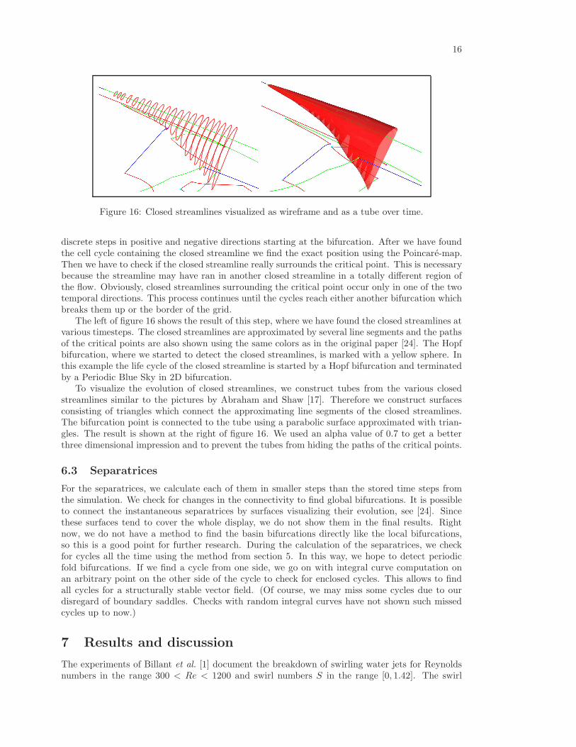
Figure 16: Closed streamlines visualized as wireframe and as a tube over time.

discrete steps in positive and negative directions starting at the bifurcation. After we have foundthe cell cycle containing the closed streamline we find the exact position using the Poincare-map.Then we have to check if the closed streamline really surrounds the critical point. This is necessarybecause the streamline may have ran in another closed streamline in a totally different region ofthe flow. Obviously, closed streamlines surrounding the critical point occur only in one of the twotemporal directions. This process continues until the cycles reach either another bifurcation whichbreaks them up or the border of the grid.

The left of figure 16 shows the result of this step, where we have found the closed streamlines atvarious timesteps. The closed streamlines are approximated by several line segments and the pathsof the critical points are also shown using the same colors as in the original paper [24]. The Hopfbifurcation, where we started to detect the closed streamlines, is marked with a yellow sphere. Inthis example the life cycle of the closed streamline is started by a Hopf bifurcation and terminatedby a Periodic Blue Sky in 2D bifurcation.

To visualize the evolution of closed streamlines, we construct tubes from the various closedstreamlines similar to the pictures by Abraham and Shaw [17]. Therefore we construct surfacesconsisting of triangles which connect the approximating line segments of the closed streamlines.The bifurcation point is connected to the tube using a parabolic surface approximated with trian-gles. The result is shown at the right of figure 16. We used an alpha value of 0.7 to get a betterthree dimensional impression and to prevent the tubes from hiding the paths of the critical points.

6.3 Separatrices

For the separatrices, we calculate each of them in smaller steps than the stored time steps fromthe simulation. We check for changes in the connectivity to find global bifurcations. It is possibleto connect the instantaneous separatrices by surfaces visualizing their evolution, see [24]. Sincethese surfaces tend to cover the whole display, we do not show them in the final results. Rightnow, we do not have a method to find the basin bifurcations directly like the local bifurcations,so this is a good point for further research. During the calculation of the separatrices, we checkfor cycles all the time using the method from section 5. In this way, we hope to detect periodicfold bifurcations. If we find a cycle from one side, we go on with integral curve computation onan arbitrary point on the other side of the cycle to check for enclosed cycles. This allows to findall cycles for a structurally stable vector field. (Of course, we may miss some cycles due to ourdisregard of boundary saddles. Checks with random integral curves have not shown such missedcycles up to now.)

7 Results and discussion

The experiments of Billant et al. [1] document the breakdown of swirling water jets for Reynoldsnumbers in the range 300 < Re < 1200 and swirl numbers S in the range [0, 1.42]. The swirl

17

number S is defined by [1]

S ≡2vθ(R/2, z0)

vz(0, z0)(21)

where z0 = 0.4D, D = 2R being the nozzle diameter. The Reynolds number is

Re ≡vz(0, z0)D

ν(22)

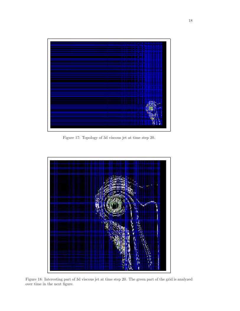
The simulation of the 3d viscous flow calculates the values on a cylindrical grid. From this grid,we only take the values on a halfplan with the axis of the cylinder as one side and the radius as theother side. This results in an cartesian grid due to the set up of the direct numerical simulation.In figure 17, one can see the topology of the instantaneous integral curves after 20 timesteps. Thefigure does not show the whole grid but most of it. It is not difficult to see that the whole actiontakes place in a small area in the lower right corner. One can see vortical motion in action andmight ask for a closer look at the critical points and cycles. For a better analysis, it may bementioned that the program sets very small values to zero at the vertices to avoid a large numberof critical points in the empty zone of the grid that may occur from numerical errors. If the valuesare very close to zero, the simulation method creates a large number of extremely weak criticalpoints that do not have any physical significance, but result in a very disturbing visualization.In figure 18, we present a closer look at the topological structure of the flow. The flow does notcontain a cycle right now, but one can see various blue sinks and green sources. All the curvesare separatrices created by the red colored saddle points. The green part of the grid around thedominant structure in the middle is now used for an analysis of the topology evolution. We showthis evolution in figure 19. The cone below shows the direction of time from time step 20 at thecircle to time step 70 at the top. One can see clearly the paths of the saddles, sinks, and sources.All the small spheres stand for bifurcations. A static fold is shown by a purple sphere. A lightblue sphere shows its inverse, i.e. a pairwise creation of a sink and a saddle or a source and asaddle. The yellow spheres denote Hopf bifurcations. As before, the transparent red surfaces showthe evolution of cycles. They can either end/start at a Hopf bifurcation or at a blue sky in 2dbifurcation. As mentioned before, we have found no evidence for periodic fold bifurcations. Sincewe do not show the separatrices, one can also not see basin bifurcations.

We use the axisymmetric simulation to indicate some of the problems that we still have to solve.Figure 20 shows a large number of Hopf bifurcations along the trace of some of the sinks/sources.This is difficult for the analysis since it is nearly impossible to check for the cycles created (anddestroyed) by these bifurcations. We present also a close-up in figure 21. Here, one can see thatthere are also sometimes larger number of static fold bifurcations that one would like to ignoresince they are obviously not important for the behavior of the flow.

8 Conclusions

The analysis of the vector field topology based on instant vector lines, called streamlines, in planesections of either axi-symmetric or three dimensional flows was developed. The vector fields weregenerated as solutions of the Navier-Stokes equations in cylindrical coordinates for swirling jetflows at moderate Reynolds numbers and supercritical swirl numbers, that produce recirculationand breakdown. The results for axi-symmetric flows develop a dense population of critical pointsand limit cycles as a result of flow normal to the plane considered. The temporal analysis using asequence of planar (r − z plane) snapshots of the early stage of a fully three dimensional swirlingjet show the emergence of Hopf and blue sky bifurcations but no periodic fold bifurcation. Theextension of the numerical tools for the topological analysis of vector fields to three dimension iscurrently under way and it can be expected that they will contribute to the understanding of theproperties of turbulent fields. In particular the number of critical points in three dimensions is ofinterest, since it has been conjectured that it is much smaller than in two dimensional flows.

18

Figure 17: Topology of 3d viscous jet at time step 20.

Figure 18: Interesting part of 3d viscous jet at time step 20. The green part of the grid is analyzedover time in the next figure.

19

Figure 19: Evolution of the topology in the marked area over time.

Figure 20: Cascade of Hopf bifurcations in the axisymmetric case.

20

References

[1] P. Billant, J. Chomaz and P. Huerre (1999), ”Experimental study of vortex breakdown inswirling jets”, J. Fluid Mech, 376: 183-219.

[2] V. Shtern and F. Hussain (1996), ”Hysteresis in swirling jets”, J. Fluid Mech., 309, 1-44

[3] R. Fernandez-Feria, J. Fernandez de la Mora and A. Barrero (1995), ”Solution breakdown in afamily of self-similar vortices”, J. Fluid Mech., 307, 77-94

[4] V. Shtern and F. Hussain (1998), ”Instabilities of conical flows causing steady bifurcations”, J.Fluid Mech., 366, 33-85

[5] V. Shtern and F. Hussain (1999), ”Collapse, symmetry breaking and hysteresis in swirlingflows”, in Annu. Rev. Fluid Mech., vol. 31, Annual Reviews, 537-566

[6] V. Shtern, F. Hussain and M. Herrada (2000), ”New features or swirling jets”, Physics Fluids12, 2868-2877

[7] A.T. Fomenko (1987), ”The topology of surfaces of constant energy in integrable Hamiltoniansystems and obstructions to integrability”, Math. USSR Izv. 29, 629-658.

[8] A.T. Fomenko (1991), ”The Theory of Invariants of Multidimensional Integrable HamiltonianSystems”, Advances in Soviet Mathematics 6, 1-35.

[9] W. Kollmann and J.Y. Roy (2000), ”Hybrid Navier-Stokes solver in cylindrical coordinates I:Method”, Computational Fluid Dynamics Journal 9, 1-16.

[10] W. Kollmann and J.Y. Roy (2000), ”Hybrid Navier-Stokes solver in cylindrical coordinatesII: Validation”, Computational Fluid Dynamics Journal 9, 17-22.

[11] Canuto, C., Hussaini, M.Y. and Zang, T.A. (1988), ”Spectral Methods in Fluid Dynamics”,Springer-Verlag, Berlin.

[12] H.R. Lewis and P.M. Bellan (1990), ”Physical constraints on the coefficients of Fourier expan-sions in cylindrical coordinates”, J. Math. Phys. 31: 2592-2596.

[13] H. Eisen and W. Heinrichs and K. Witsch (1991), ”Spectral collocation methods and polarcoordinate singularities”, J. Comput. Physics 96, 241-257

[14] C.A. Kennedy and M.H. Carpenter (1994), ”Several new numerical methods for compressibleshear layer simulations”, Appl. Num. Math. 14, 397-433

[15] Li, Y. (1997), ”Wavenumber Extended High-Order Upwind-Biased Finite Difference Schemesfor Convective Scalar Transport”, J. Comput. Phys. 133: 235-255.

[16] J.J. Dongarra and C.B. Moler and J.R. Bunch and G.W. Stewart (1979), ”LINPACK user’sguide”, SIAM Philadelphia

[17] R. H. Abraham and C. D. Shaw (1982,1983,1985,1988), “Dynamics, the Geometry of BehaviorI–IV”, Aerial Press, Santa Cruz, CA.

[18] J. Guckenheimer and P. Holmes (1983), “Dynamical systems and bifurcation of vector fields”,Springer-Verlag, New York, NY.

[19] M. W. Hirsch and S. Smale !974), “Differential equations, dynamical systems and linear alge-bra”, Academic Press, New York, NY.

[20] S. Lang (1995), “Differential and Riemannian manifolds”, Springer, New York, third edition.

[21] W. H. Press, S. A. Teukolsky, W. T. Vetterling, and B. P. Flannery !992), “Numerical Recipesin C”, Cambridge University Press, Cambridge, UK, 2nd edition.

21

[22] G. Scheuermann, B. Hamann, K. I. Joy, and W. Kollmann (2000), “Visualizing local vectorfield topology”, Journal of Electronic Imaging 9(4):356 – 367.

[23] X. Tricoche, G. Scheuermann, and H. Hagen (2000), “A topology simplification method for2d vector fields”, In IEEE Visualization 2000, IEEE Computer Society, Los Alamitos, CA, 359– 366.

[24] X. Tricoche, G. Scheuermann, and H. Hagen (2001), “Topology-Based Visualisation Of Time-Dependent 2D Vector Fields”, In Joint Eurographics and IEEE TCVG Symposium on Visual-ization 2001, Springer, Wien, 117 – 126.

22

Figure 21: Zoom into some of the cascades.