Research paperDOI 10.1007/s00158-003-0322-7Struct Multidisc Optim 26, 295–307 (2004)

Reliability-based topology optimization

G. Kharmanda, N. Olhoff, A. Mohamed and M. Lemaire

Abstract The objective of this work is to integratereliability analysis into topology optimization problems.The new model, in which we introduce reliability con-straints into a deterministic topology optimization for-mulation, is called Reliability-Based Topology Optimiza-tion (RBTO). Several applications show the importanceof this integration. The application of the RBTO modelgives a different topology relative to deterministic top-ology optimization. We also find that the RBTO modelyields structures that are more reliable than those pro-duced by deterministic topology optimization (for thesame weight).

Key words reliability-based topology optimization,reliability-based design optimization, reliability analysis,sensitivity analysis, finite element analysis

1Introduction

Reliability-based optimization aims to define the bestcompromise between cost and safety. One reliability-based model is Reliability-Based Design Optimization(RBDO), which allows structures to be designed. For the

Received: 25 October 2002Published online: 23 December 2003 Springer-Verlag 2003

G. Kharmanda1, N. Olhoff2,, A. Mohamed3 andM. Lemaire3

1 Faculty of Mechanical Engineering, Aleppo, Syriae-mail: gh_kharmanda@hotmail.com2 Institute of Mechanical Engineering, Aalborg University,DK-9220, Aalborg East, Denmarke-mail: no@ime.auc.dk3 LaRAMA-IFMA/UBP, Campus de Clermont-Ferrand, BP265, 63175 Aubiere, Francee-mail: alaa.mohamed@ifma.fr, maurice.lemaire@ifma.fr

Research carried out during the first author’s visit to the In-stitute of Mechanical Engineering, Aalborg, November 2001 –February 2002

RBDO model, the coupling between geometrical model-ing, mechanical simulation, reliability analyses, and opti-mization methods leads to very long computing times andweak convergence stability. Traditionally, the solution ofthe RBDO model is achieved by alternating reliabilityand optimization iterations (sequential approach). Thisapproach leads to low numerical efficiency, which is dis-advantageous for engineering applications on real struc-tures. In order to avoid this difficulty, an efficient methodwas proposed by Kharmanda et al. (2001a, 2002c), whichis called the hybrid (or concurrent) RBDO method. Thismethod is based on the simultaneous solution of the relia-bility and the design optimization problem.Furthermore, in the shape optimization case, when in-

tegrating the reliability analysis into the optimization ofgeometrical shape variables, CAD model updating is ne-cessary during the design phase. Then, the parametriza-tion step allows the search directions of the optimizationprocess to be defined. Parameters defining points and di-rections are chosen among the design variables that definethe geometry of the domain boundary. The shape opti-mization process is directed by the information corres-ponding to the geometrical boundary perturbation. Thestructural geometry to be modified during the optimiza-tion process can be defined by several descriptions, suchas Bezier, B-spline, or NURBS models (Kharmanda et al.2002a,b). This model is called Reliability-Based ShapeOptimization (RBSO).In deterministic topology optimization, the designer

aims to obtain the solution without taking into ac-count the effects of uncertainties concerning geometryand loading given by deterministic variables. The inte-gration of the reliability or safety criteria into the top-ology optimization presents a new type of optimizationcalled Reliability-Based Topology Optimization (RBTO)(Kharmanda and Olhoff 2001b). The purpose of RBTOis to take into account the randomness of the appliedloads and the description of the geometry. It also providesthe designer with several solutions. Using the RBTOmodel, we obtain different topologies compared with thedeterministic topology optimization procedure. The re-sulting topologies depend on the target reliability levels.The shape optimization algorithm can be applied to bet-ter control the solution. The resulting structures present

296

a better volume/reliability ratio than the determinis-tic ones. In this paper, we first present the reliabilityanalysis and the importance of its integration with thetopology optimization problem. The deterministic top-ology optimization formulation and the RBTOmodel willbe presented next. The RBTO procedure will then be de-tailed and several examples will show the applicability ofthe new model. Some reliability-based topologies for dif-ferent reliability levels will finally be presented as newresulting topologies.

2Reliability analysis

The design of structures and the prediction that theyfunction well lead to the verification of a number of rulesresulting from the knowledge of physical and mechanicalexperience by designers and constructors. These rules ex-plain the necessity to limit loading effects such as stressesand displacements. Each rule represents an elementaryevent and the occurrence of several events leads to a fail-ure scenario. The objective is then to evaluate the fail-ure probability corresponding to the occurrence of criticalfailure modes.

2.1Importance of safety criteria

In deterministic structural optimization, the designeraims to reduce the construction cost without taking theeffects of uncertainties concerning materials, geometry,and loading into account. In this way, the resulting opti-mal configuration may represent a lower reliability leveland then lead to a higher failure rate. The balance be-tween cost minimization and reliability maximization isa great challenge to the designer. The interest in reliabil-ity criteria in design optimization is to improve the reli-ability level of the system without increasing its weightsignificantly. But when integrating reliability into top-ology optimization problems, the interest is to provide thedesigner with several topologies by considering the ran-domness of the main variables of the structure. In RBDOmodels, we distinguish between two kinds of variables:

1) The design variables x, which are deterministic vari-ables to be defined in order to optimize the design.They represent the control parameters of the mechan-ical system (e.g. dimensions, materials, loads) andof the probabilistic model (e.g. means and standard-deviations of the random variables);

2) The random variables y, which represent the struc-tural uncertainties, identified by probabilistic distri-butions. These variables can be geometrical dimen-sions, material characteristics, or the applied externalloading. These two kinds of variables (x and y) can berelated by a probabilistic transformation.

However, in the RBTO model, the random and designvariables are not related, because the design variables xare the densities of material of the discretization elem-ents, while the random variables y are related to knownquantities. Hence, we have three kinds of variables:

1) The deterministic topology design variables x, whichare deterministic variables;

2) The random variables y, which represent the struc-tural uncertainties, identified by probabilistic distri-butions. These variables can be geometrical dimen-sions, material characteristics, or the applied externalloading;

3) The normalized variables u, which relate the ran-dom variables and their mean values and standard-deviations.

2.2Failure probability

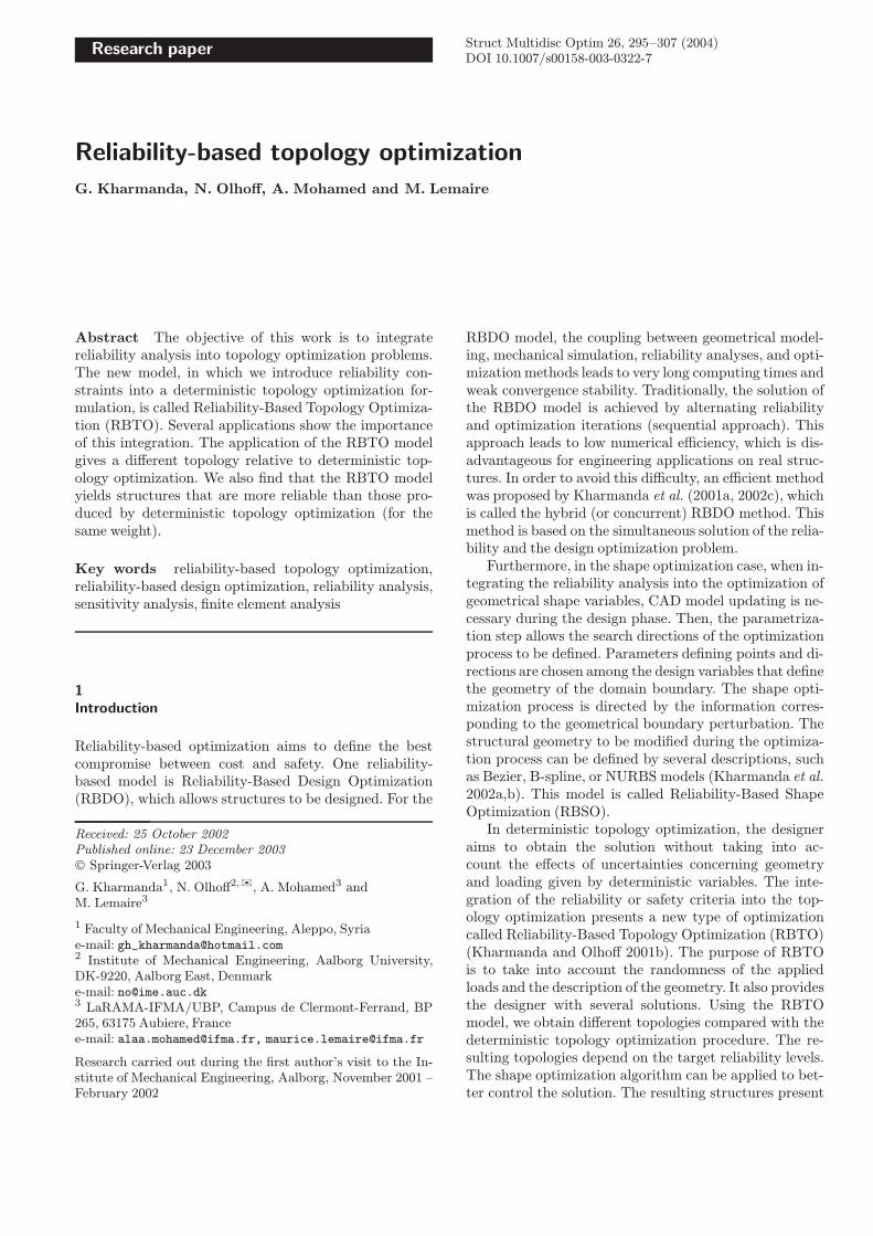
In addition to the vector of deterministic variables x tobe used in the system design and optimization, the un-certainties are modeled by a vector of stochastic physicalvariables affecting the failure scenario. The knowledge ofthese variables is not, at best, more than statistical in-formation and we admit a representation in the form ofrandom variables. For a given design rule, the basic ran-dom variables are defined by their joint probability dis-tribution associated with some expected parameters; thevector of random variables is denoted herein by Y, therealizations of which are written as y. Safety is the statein which the structure is able to fulfil all the functioningrequirements (e.g. strength and serviceability) for whichit is designed. To evaluate the failure probability with re-spect to a chosen failure scenario, a limit state functionG(x,y) is defined by the condition of good functioning ofthe structure. In Fig. 1, the limit between the state offailure G(x,y)< 0 and the state of safety G(x,y)> 0is known as the limit state surface G(x,y) = 0. Thefailure probability is then calculated by

Pf = Pr [G (x,y)≤ 0] =

∫

G(x,y)≤0

fY(y) dy1 · · · dyn , (1)

wherePf is the failure probability, fY (y) is the joint dens-ity function of the random variables Y, and Pr[.] is theprobability operator. The evaluation of the integral in (1)is not easy, because it represents a very small quantityand all the necessary information for the joint densityfunction are not available. For these reasons, the Firstand Second Order Reliability Methods FORM/SORM(Ditlevsen and Madsen 1996) were developed. They arebased on the reliability index concept, followed by an es-timation of the failure probability. The invariant reliabil-ity index β was introduced by Hasofer and Lind (1974),who proposed working in the space of standard indepen-dent Gaussian variables instead of the space of physicalvariables.

297

Fig. 1 Physical and normalized spaces

The transformation from the physical variables y tothe normalized variables u is given by

u= T (x, y) and y= T−1(x,u) .

The operator T (.) is called the probabilistic transform-ation. In this standard space, the limit state functiontakes the form

H(x,u)≡G(x,y) = 0 . (2)

In the FORM approximation, the failure probability issimply evaluated by:

Pf ≈ Φ(−β) , (3)

where Φ(.) is the standard Gaussian cumulated function.For practical engineering, (3) gives a sufficiently accurateestimation of the failure probability.

2.3Reliability evaluation

For a given failure scenario, the reliability index β isevaluated by solving a constrained optimization problem(Fig. 1).The calculation of the reliability index can be realized

by the following form:

β =min(√uTu)subject to H(x,u) ≤ 0 . (4)

The solution of this problem is called the design pointP ∗, as illustrated in Fig. 1. When the mechanical modelis defined by numerical methods such as the finite elementmethod, the evaluation of the reliability implies a specialcoupling procedure between both reliability and mechan-ical models (Lemaire and Mohamed 2000).

3Deterministic topology optimization

Deterministic topology optimization has a great impacton the performance of structures, and the last decadehas seen an enormous interest in this important sub-areaof structural optimization (Bendsøe and Kikuchi 1988;Bendsøe 1995; Olhoff et al. 1998; Rozvany 2000; Olhoff2000; Rozvany and Olhoff 2000; Eschenauer and Olhoff2001). For deterministic topologies, we can find severalapproaches for solving topology optimization problems.The homogenization approach was used in Bendsøe andKikuchi (1988), based on studies of the existence of so-lutions. This approach has been adopted in many pa-pers, but has the disadvantage that the determinationand the evaluation of optimal microstructures and theirorientations is cumbersome if not unresolved (for otherthan compliance problems) and, furthermore, the result-ing structures cannot be built since no definite length-scale is associated with the microstructures. However,the homogenization approach to topology optimization isstill important in the sense that it can provide boundson the theoretical performance of structures. A topologyoptimization problem based on the homogenization ap-proach, with the objective of minimizing the compliance(thereby maximizing the integral structural stiffness),subject to an upper bound on the volume, can be writtenas

min L (w)

subject to ad (w, v) = L(v) for all v ∈H

and volume≤ V0 (5)

with

L(v) =

∫

Ω

f v dΩ+

∫

Γ

t v dΓ (6)

and

ad(w, v) =

∫

Ω

Cijkl(d)εij(w)εkl(v)dΩ , (7)

where f and t are, respectively, the body force and sur-face traction, εij is the strain tensor, Cijkl is the effectivestiffness tensor of the microstructure cells, and H is theset of kinematically admissible displacement fields. Theproblem is defined on a fixed reference domain Ω and thestiffness Cijkl depends on the design variables used.

298

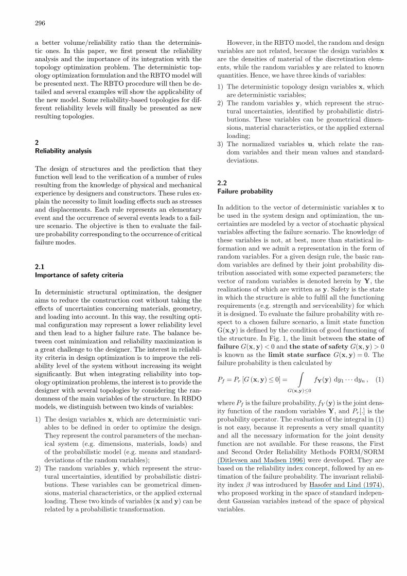
Fig. 2 Density variables in microstructure cells

For a so-called second-rank layering, such as the thirdcell in Fig. 2, we have the relationship

Cijkl ≡ Cijkl(µ, γ, θ) , (8)

where µ and γ denote the dimensions of the layering andθ is the rotation angle of the layering. The relation (8) canbe computed analytically and the volume is evaluated by

volume =

∫

Ω

(µ+γ−µγ)dΩ . (9)

Alternative microstructures such as square or rectangularholes in square cells can also be used (such as the first twocells in Fig. 2), the important feature being the possibil-ity of having density values covering the full interval [0,1].The optimization problem can now be solved either byoptimality criteria methods or by duality methods, wherethe advantage is to take into account the fact that theproblem has just one constraint. The angle θ of layer ro-tation is controlled via the results on the optimal rotationof orthotropic materials as presented in Pedersen (1989,1991) and Hassani and Hinton (1999).Another approach is called the SIMP approach (Solid

Isotropic Microstructure with Penalty) or power-law ap-proach (Bendsøe 1989; Zhou and Rozvany 1991; Mlejnek1992). Here, material properties are assumed to be con-stant within each element used to discretize the designdomain and the variables are the relative densities ofthe elements. The material properties are modeled as therelative material properties of the solid material. Thisapproach has been criticized, since it was argued thatno physical material exists with properties described bythe power-law interpolation. However, a recent paper byBendsøe and Sigmund (1999) proved that the power-lawapproach is physically permissible as long as simple con-ditions for the power are satisfied (e.g. p ≥ 3 for Pois-son’s ratio equal to 1/3). To ensure the existence of solu-tions, the power-law approach to topology optimizationhas been applied to problems with multiple constraints,multiple physics, and multiple materials.A topology optimization problem based on the power-

law approach, in which the objective is to minimize com-pliance, can be written as

min C(x) = qTKq=N∑e=1

(xe)pqTe k0qe

subject toV (x)

V0≤ f ,

Kq= F ,

0< xmin ≤ x≤ 1 , (10)

where q and F are the global displacement and force vec-tors, respectively,K is the global stiffness matrix, qe andk0 are the element displacement vector and stiffness ma-trix, respectively, x is the vector of design variables, xminis a vector of minimum relative densities (non-zero toavoid singularity), N is the number of elements to dis-cretize the design domain, p is the penalization power,V (x) and V0 are the material volume and design do-main volume, respectively, and f is a prescribed upperbound on the volume fraction. Whereas the solution ofthe above-mentioned approaches is based on mathemati-cal programming techniques and continuous design vari-ables, a number of papers have appeared on solving thetopology optimization problem as an integer problem.Beckers successfully solved large-scale compliance mini-mization problems (Beckers 1999) using a dual-approach,but other approaches based on genetic algorithms orother heuristic approaches require thousands of functionevaluations even for a small number of elements and mustbe considered impractical.

4RBTO

Size, shape, and topology optimization problems addressdifferent aspects of a structural design problem. In a typ-ical sizing problem the goal may be to find the opti-mal thickness distribution of a segmented linearly elas-tic plate. The optimal thickness distribution minimizes(or maximizes) a physical quantity such as the compli-ance (external work), peak stress, deflection, etc., whileequilibrium and other constraints on the state and de-sign variables are satisfied. The main feature of the sizingproblem is that the domain of the design model and state

299

variables is known a priori and is fixed throughout theoptimization process.On the other hand, in a shape optimization problem

the goal is to find the optimum shape of this domain,that is, the shape problem is defined on a variable do-main. Topology optimization of solid structures involvesthe determination of features such as the number and lo-cation of holes and the connectivity of the domain. Thelayout problem that shall be defined in the following com-bines several features of the traditional problems in struc-tural design optimization (Bendsøe 1995). However, theintegration of the reliability analysis in each step of thestructural design optimization plays an important role byconsidering the variability of the most sensitive variables.This variability or randomness has to be considered in theoptimization processes in order to reduce the structuralweight in the uncritical regions and hence to producestructures that are reliable and economic. The appliedloads are very often considered as random variables be-cause they participate strongly in the failure or damage.Similarly, the geometry and the materials can be mod-eled as random variables. The purpose of reliability-basedlayout optimization is to find the reliable and optimallayout of a structure within a specified region. In the de-terministic design optimization problem, the only knownquantities are the applied loads, the possible support con-ditions, the volume of the structure to be constructed,and possibly some additional design specifications such asthe location and size of prescribed holes. But the physicalsize and shape and the connectivity of the structure areunknown.When introducing the reliability, the user chooses

some known quantities that will be random variables.They are initially set to their mean values. Then they takerandom realizations during the optimization process.

4.1Formulation

The main difference between the deterministic topologyoptimization procedure and the proposed RBTOmodel isthat the randomness (variability) of the most importantvariables that exhibit a strong influence on the resultingoptimal topology is taken into account. The determinis-tic topology problem allows for the prediction of the grossshape of the body and it is possible to predict the place-ment and shapes of holes in the structure. However, theRBTO model leads to a different set of optimal topolo-gies with respect to that produced by the deterministictopology optimization procedure. In order to control thetopologies produced, a reliability index β (see Hasoferand Lind 1974) is introduced with a normalized vector u.In the case of a normal distribution, u is given by

uj =yj−myjσyj

, (11)

with

β =min√u21+ ...+u

2j+ ...+u

2J subject to G≤ 0 ,

where yj is the j-th random variable, with mean valuemyj and standard-deviation σyj , and G is the limit statefunction. J is the number of selected random variables.In (11), the vector u defines the relationship between therandom variables and the design variables.The RBTO problem consists of minimizing the com-

pliance subject to a given upper bound on the volumeof material and the reliability constraints. The mate-rial density is used as a continuous design variable. TheRBTO formulation based on the homogenization ap-proach can be expressed as

min L (w)

subject to β(u)≥ βt ,

ad (w, v, u) = L(v, u) for all v ∈H ,

volume≤ V0 , (12)

with

L(v, u) =

∫

Ω

f(u) v dΩ+

∫

Γ

t(u) v dΓ

and

ad(w, v, u) =

∫

Ω

Cijkl(d, u)εij(w, u)εkl(v)dΩ .

However, using the SIMP approach, the problem can bewritten as

min C(x) = qTKq=N∑e=1

(xe)pqTe k0qe

subject to β(u)≥ βt ,

K(x,y,u) ·q(x,y,u) = F(y,u) ,

V (x,y,u)

V0≤ f ,

0< xmin ≤ x≤ 1 , (13)

where β and βt are the reliability index of the system andthe target reliability index, respectively. (12) and (13)define problems called Reliability-Based Topology Opti-mization (RBTO) problems. For example, in (12) and(13), the loading and the geometry play an importantrole in the performance of the structure. Therefore, usingthe RBTO model, we consider the dimensions and loadsas random variables. In this work, we apply the RBTOformulation in (13) based on the SIMP approach. The de-sign variables x are the densities of material in each ofthe finite elements, while the random variables y are theexternal loads and the geometric dimensions. Since thevolume fraction of the structure directly depends on thegeometric dimensions, it can be included in the set of se-lected random variables.

300

4.2RBTO algorithm

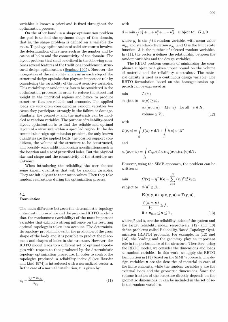
Figure 3 presents the RBTO algorithm as a sequentialprocedure that constitutes an iterative loop that is re-peated until convergence. The RBTO model containsthree principal successive processes: sensitivity analysis,reliability index evaluation, and the topology optimiza-tion process. Each one of these processes is considered asan independent loop that does not lead to a long com-putational time relative to the deterministic topology op-

Fig. 3 RBTO procedure constituting an iterative loop thatis repeated until convergence

timization scheme. This procedure is more appropriatethan the coupled procedures used in the RBDO model,which contains nested optimization and reliability loops.In the RBDO field, several papers have studied the

integration of reliability analysis into optimization prob-lems (Stevenson 1967; Moses 1977; Feng and Moses 1986;Cheng et al. 1998). All the uncertain quantities can bemodeled as random variables, and two spaces (Fig. 1) arerequired to carry out this integration. Hence, a lot of nu-merical computations are required in the space of the ran-dom variables in order to evaluate the system reliability.Furthermore, the optimization process itself is executedin the space of the design variables, which is determinis-tic. Consequently, in order to search for an optimal struc-ture, the design variables are repeatedly changed, andeach set of design variables corresponds to a new randomvariable space, which then needs to be manipulated toevaluate the structural reliability at that point. Becausetoo many repeated searches are needed in the above twospaces, the computational time for such an optimizationis a big problem.When applying the principle of this approach to top-

ology optimization, the problem becomes bigger becausethe computational time will increase significantly and thereliability analysis in each iteration of the topology op-timization procedure will represent a very complex task.Thus, we define a new different strategy, which impliesa coupling between the reliability analysis and the top-ology design problem without increasing the computa-tional time.First, we propose a set of variables assembled in the

vector my, which will be called the mean variable vec-tor, and which concerns the applied loads and geometryof the structure. But, in order to select the most effi-cient variables, we study the sensitivity of the objectivefunction with respect to the means of the proposed setof variables. The selected variables are assembled in therandom variables vector y. Secondly, the reliability indexβ is evaluated in satisfying the associated reliability con-straint, and the resulting normalized vector u is used toformulate the random variables vector y. Finally, usingthe resulting vector y, we apply the SIMP approach toobtain the new reliable and optimal topology (Fig. 3).

4.2.1Sensitivity analysis

In general, reliability-based optimization can be consid-ered as a multi-objective (or -constraint) optimizationbecause we have a principal objective function (cost, vol-ume, etc.) and an associated one (reliability index or fail-ure probability). In the case of our RBTO model, theproposed variables that are random play an importantrole in the reliability index function, but they do not nec-essarily play the same role in the compliance function.Therefore, it is necessary to find the sensitivity of the

compliance function with respect to the chosen variables.

301

Furthermore, the signs of the resulting gradients showthe influence of each variable (negative or positive) onthe objective function. The sensitivity analysis step canthen improve the performance of the structure duringthe optimization process in order to yield a more reliablestructure.The sensitivity of the compliance with respect to the

chosen means my of the geometry and applied loadscan be calculated by several methods. The simplest oneis the finite difference approach, e.g. considering that∆myjmyj

= 0.01.

Using the classical finite difference approach, we canwrite

∂C

∂myj=∆C

∆myj=C(myj +∆myi

)−C(myj

)

∆myj. (14)

(14) is very simple to implement to provide the new set ofselected variables.

4.2.2Reliability index evaluation

The evaluation of the reliability index β can be carriedout by a particular optimization procedure. This indexis the minimum distance between the limit state and theorigin in the normalized space (Fig. 1). The problem isgiven by

β =min d(u) =√∑

u2j subject to β(u)≥ βt . (15)

During the optimization procedure, we can analyticallyprovide the derivative of the distance d with respect to ujby

∂d

∂uj=uj

d(u). (16)

The resulting vector u of the problem in (15) will be usedto evaluate the random vector y by using (11) with thestandard deviations given by σyj = 0.1×myj and by con-sidering that uj has the same sign as the correspondinggradient ∂C/∂myj .

4.2.3Topology optimization procedure

After satisfying the reliability constraints and determin-ing the vector of the random variables, we call the top-ology optimization procedure with a new set of knownquantities. The resulting optimal topology principally de-pends on the reliability index value. This procedure sat-isfies the other constraints but with consideration of therandomness of the principal variables of the structure.Figure 3 shows the different steps of the algorithm of thenew Reliability-Based Topology Optimization model.

5Applications

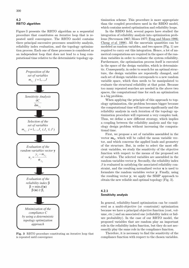
In order to illustrate the functioning and the importanceof the proposed new model, we apply the deterministictopology optimization procedure and the RBTOmodel toseveral examples shown in Figs. 4a, 5a, 6a, and 7a. Thefirst and the second examples represent aMBB-beam (seeOlhoff et al. 1991) and a cantilever beam under a sin-gle external load (Figs. 4a and 5a, respectively). Thethird example is a cantilever beam with two load-cases(Fig. 6a), and the fourth example represents a cantileverbeam with a prescribed hole (Fig. 7a). The objective ofthe following presentation is to show now the difference

Fig. 4 Example 1, topology optimization and RBTO ofthe MBB-beam: (a) full design domain, (b) half design do-main with symmetry boundary conditions, (c) resulting deter-ministic topology optimized beam, and (d) resulting RBTOstructure

302

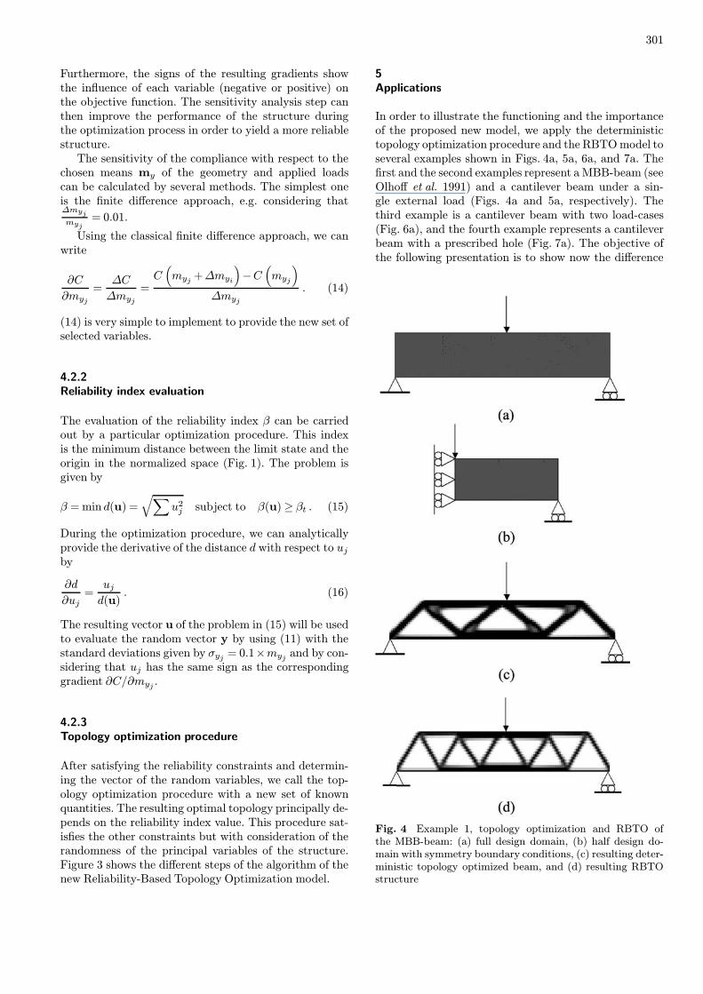
Fig. 5 Example 2, topology optimization of a cantileverbeam: (a) design domain, (b) deterministic topology opti-mized beam, and (c) corresponding reliability-based topology

between the deterministic topologies and those obtainedby the proposed new model.

5.1Topology optimization approach

Sigmund (2001) presented a compact Matlab implemen-tation of the deterministic topology optimization code forcompliance minimization of statically loaded structures.This Matlab code can be downloaded from the web-

site http://www.topopt.dtu.dk. A number of simplifica-tions are introduced to facilitate the implementation inMatlab. First, the design domain is assumed to be rectan-gular and discretized by square finite elements. This waythe numbering of elements and nodes is simple (columnby column starting in the upper left corner), and the as-pect ratio of the structure is given by the ratio of elementsin the horizontal and the vertical direction. A topologyoptimization problem based on the SIMP approach is im-plemented using (10). The optimization problem is solvedby the use of a standard optimality criteria method. Themain program is called from the Matlab prompt by theline

top(nelx,nely,volfrac,penal,rmin) ,

where nelx and nely are the numbers of elements in thehorizontal and vertical directions, respectively, volfrac is

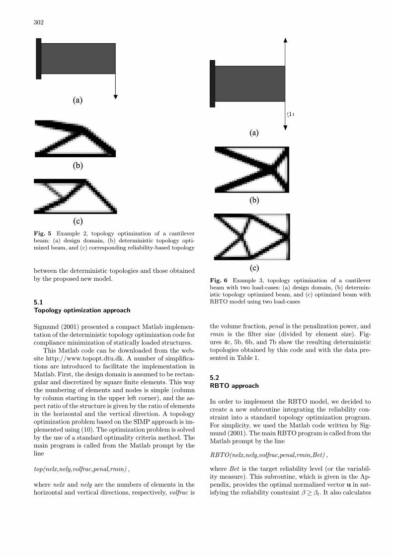
Fig. 6 Example 3, topology optimization of a cantileverbeam with two load-cases: (a) design domain, (b) determin-istic topology optimized beam, and (c) optimized beam withRBTO model using two load-cases

the volume fraction, penal is the penalization power, andrmin is the filter size (divided by element size). Fig-ures 4c, 5b, 6b, and 7b show the resulting deterministictopologies obtained by this code and with the data pre-sented in Table 1.

5.2RBTO approach

In order to implement the RBTO model, we decided tocreate a new subroutine integrating the reliability con-straint into a standard topology optimization program.For simplicity, we used the Matlab code written by Sig-mund (2001). The main RBTO program is called from theMatlab prompt by the line

RBTO(nelx,nely,volfrac,penal,rmin,Bet) ,

where Bet is the target reliability level (or the variabil-ity measure). This subroutine, which is given in the Ap-pendix, provides the optimal normalized vector u in sat-isfying the reliability constraint β ≥ βt. It also calculates

303

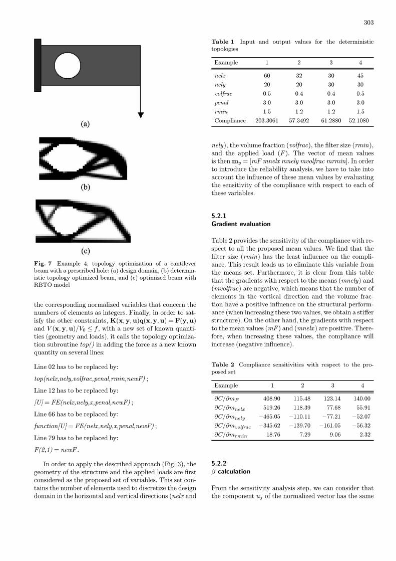
Fig. 7 Example 4, topology optimization of a cantileverbeam with a prescribed hole: (a) design domain, (b) determin-istic topology optimized beam, and (c) optimized beam withRBTO model

the corresponding normalized variables that concern thenumbers of elements as integers. Finally, in order to sat-isfy the other constraints, K(x,y,u)q(x,y,u) = F(y,u)and V (x,y,u)/V0 ≤ f , with a new set of known quanti-ties (geometry and loads), it calls the topology optimiza-tion subroutine top() in adding the force as a new knownquantity on several lines:

Line 02 has to be replaced by:

top(nelx,nely,volfrac,penal,rmin,newF) ;

Line 12 has to be replaced by:

[U]= FE(nelx,nely,x,penal,newF) ;

Line 66 has to be replaced by:

function[U]= FE(nelx,nely,x,penal,newF) ;

Line 79 has to be replaced by:

F(2,1) = newF .

In order to apply the described approach (Fig. 3), thegeometry of the structure and the applied loads are firstconsidered as the proposed set of variables. This set con-tains the number of elements used to discretize the designdomain in the horizontal and vertical directions (nelx and

Table 1 Input and output values for the deterministictopologies

Example 1 2 3 4

nelx 60 32 30 45

nely 20 20 30 30

volfrac 0.5 0.4 0.4 0.5

penal 3.0 3.0 3.0 3.0

rmin 1.5 1.2 1.2 1.5

Compliance 203.3061 57.3492 61.2880 52.1080

nely), the volume fraction (volfrac), the filter size (rmin),and the applied load (F ). The vector of mean valuesis thenmy = [mF mnelx mnely mvolfrac mrmin]. In orderto introduce the reliability analysis, we have to take intoaccount the influence of these mean values by evaluatingthe sensitivity of the compliance with respect to each ofthese variables.

5.2.1Gradient evaluation

Table 2 provides the sensitivity of the compliance with re-spect to all the proposed mean values. We find that thefilter size (rmin) has the least influence on the compli-ance. This result leads us to eliminate this variable fromthe means set. Furthermore, it is clear from this tablethat the gradients with respect to the means (mnely) and(mvolfrac) are negative, which means that the number ofelements in the vertical direction and the volume frac-tion have a positive influence on the structural perform-ance (when increasing these two values, we obtain a stifferstructure). On the other hand, the gradients with respectto the mean values (mF ) and (mnelx ) are positive. There-fore, when increasing these values, the compliance willincrease (negative influence).

Table 2 Compliance sensitivities with respect to the pro-posed set

Example 1 2 3 4

∂C/∂mF 408.90 115.48 123.14 140.00

∂C/∂mnelx 519.26 118.39 77.68 55.91

∂C/∂mnely −465.05 −110.11 −77.21 −52.07

∂C/∂mvolfrac −345.62 −139.70 −161.05 −56.32

∂C/∂mrmin 18.76 7.29 9.06 2.32

5.2.2β calculation

From the sensitivity analysis step, we can consider thatthe component uj of the normalized vector has the same

304

Table 3 The normalized values, the reliability index, and theresulting objective function for RBTO

Example 1 2 3 4

uF 1.886 1.869 1.801 1.801

unelx 1.833 1.875 2.000 2.000

unely −2.000 −2.000 −2.000 −2.000

uvolfrac −1.886 −1.869 −1.801 −1.801

β 3.805 3.808 3.806 3.806

Compliance 980.2142 248.3102 240.7449 187.0253

sign as the corresponding gradient ∂C/∂myj . Table 3 pro-vides the normalized vector and the reliability index inconsidering the target reliability index βt = 3.8. For sim-plicity, we consider herein the limit state function as a lin-ear combination of the random variables.

5.2.3Topology optimization approach

When calling the program RBTO( ), we consider thesame input values of nelx, nely, volfrac, penal , and rmin,as presented in Table 1, but the input target reliabil-ity level has to be introduced (for these four examples:Bet= 3.8). After having evaluated the normalized vectoru, we compute the new values of the selected random vari-able vector y = [F nelx nely volfrac] using (11) and con-sidering the standard-deviations σyj = 0.1myj .Finally, in order to apply the topology optimization

based on the SIMP approach (13), the program RBTO( )will call the topology optimization code top( ), with a newset of values (data), that corresponds to the selected ran-dom variable vector y. Figures 4d, 5c, 6c, and 7(c) showthe optimal topologies based on the usage of the RBTOalgorithm. It is clear that the reliability-based topolo-gies and their resulting compliance values are differentfrom those obtained by the deterministic cases (see Ta-bles 1 and 3). In order to show the importance of thisstudy, we can apply a design optimization procedure toboth reliability-based topologies and the deterministicones under similar conditions.

5.3Importance of the RBTO model

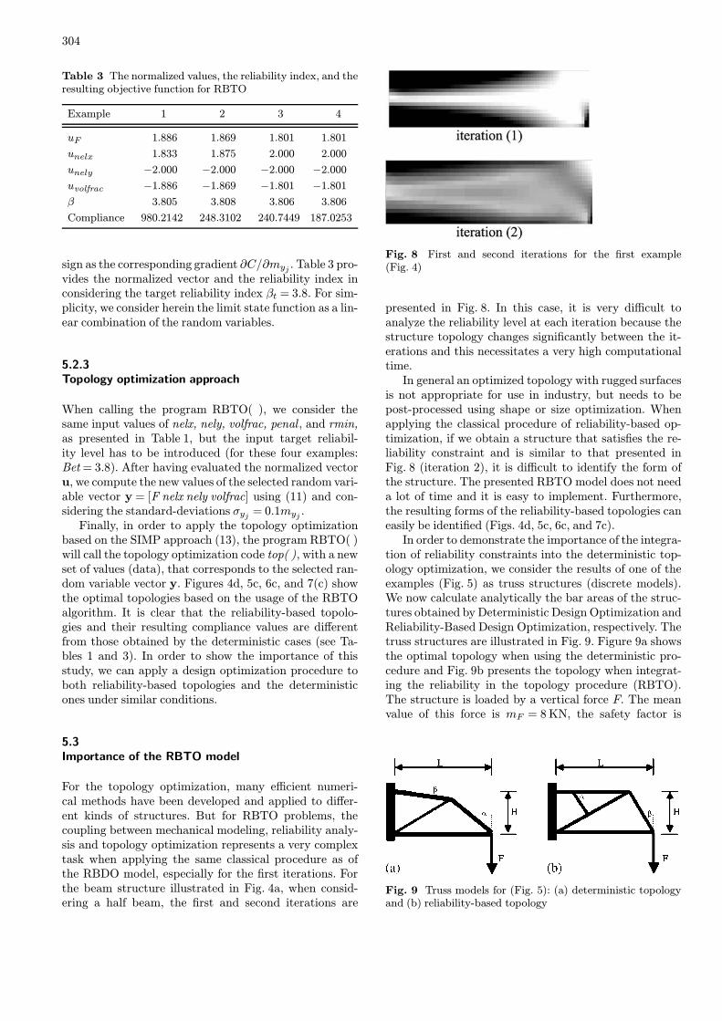
For the topology optimization, many efficient numeri-cal methods have been developed and applied to differ-ent kinds of structures. But for RBTO problems, thecoupling between mechanical modeling, reliability analy-sis and topology optimization represents a very complextask when applying the same classical procedure as ofthe RBDO model, especially for the first iterations. Forthe beam structure illustrated in Fig. 4a, when consid-ering a half beam, the first and second iterations are

Fig. 8 First and second iterations for the first example(Fig. 4)

presented in Fig. 8. In this case, it is very difficult toanalyze the reliability level at each iteration because thestructure topology changes significantly between the it-erations and this necessitates a very high computationaltime.In general an optimized topology with rugged surfaces

is not appropriate for use in industry, but needs to bepost-processed using shape or size optimization. Whenapplying the classical procedure of reliability-based op-timization, if we obtain a structure that satisfies the re-liability constraint and is similar to that presented inFig. 8 (iteration 2), it is difficult to identify the form ofthe structure. The presented RBTO model does not needa lot of time and it is easy to implement. Furthermore,the resulting forms of the reliability-based topologies caneasily be identified (Figs. 4d, 5c, 6c, and 7c).In order to demonstrate the importance of the integra-

tion of reliability constraints into the deterministic top-ology optimization, we consider the results of one of theexamples (Fig. 5) as truss structures (discrete models).We now calculate analytically the bar areas of the struc-tures obtained by Deterministic Design Optimization andReliability-Based Design Optimization, respectively. Thetruss structures are illustrated in Fig. 9. Figure 9a showsthe optimal topology when using the deterministic pro-cedure and Fig. 9b presents the topology when integrat-ing the reliability in the topology procedure (RBTO).The structure is loaded by a vertical force F. The meanvalue of this force is mF = 8KN, the safety factor is

Fig. 9 Truss models for (Fig. 5): (a) deterministic topologyand (b) reliability-based topology

305

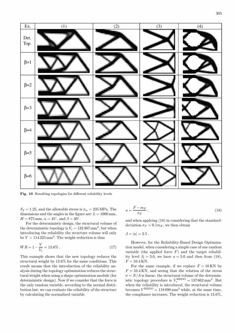
Fig. 10 Resulting topologies for different reliability levels

Sf = 1.25, and the allowable stress is σw = 235MPa. Thedimensions and the angles in the figure are:L= 1000mm,H = 875mm, α= 45, and β = 30.For the deterministic design, the structural volume of

the deterministic topology is Vc = 132367mm3, but when

introducing the reliability the structure volume will onlybe V = 114325mm3. The weight reduction is thus

WR= 1−V

Vc= 13.6% . (17)

This example shows that the new topology reduces thestructural weight by 13.6% for the same conditions. Thisresult means that the introduction of the reliability an-alysis during the topology optimization reduces the struc-tural weight when using a shape optimization module (fordeterministic design). Now if we consider that the force isthe only random variable, according to the normal distri-bution law, we can evaluate the reliability of the structureby calculating the normalized variable

u=F −mFσF

, (18)

and when applying (18) in considering that the standard-deviation σF = 0.1mF , we then obtain

β = |u|= 2.5 .

However, for the Reliability-Based Design Optimiza-tion model, when considering a simple case of one randomvariable (the applied force F ) and the target reliabil-ity level βt = 3.0, we have u = 3.0 and then from (18),F = 10.4KN.For the same example, if we replace F = 10KN by

F = 10.4KN, and seeing that the relation of the stressσ =N/A is linear, the structural volume of the determin-istic topology procedure is V RBDOc = 137662mm3. Butwhen the reliability is introduced, the structural volumebecomes V RBDO = 118898mm3 while, at the same time,the compliance increases. The weight reduction is 13.6%,

306

the same as the deterministic one. This reduction demon-strates the importance of the reliability in the topologyoptimization. This importance can also be verified whenconsidering shape and size optimization for determinis-tic optimization as well as for reliability-based optimiza-tion. In Fig. 10, the reader can see different topologiesfor different reliability levels of the four Examples 1–4 inFigs. 4–7.

6Conclusion

The proposed Reliability-Based Topology Optimization(RBTO) model aims to consider randomness (variabil-ity) of the most important quantities of a structure, suchas the geometry and the applied loads. The coupling be-tween the reliability analysis and the topology optimiza-tion is carried out by the use of a particular optimizationprocedure. The importance of the RBTO model is in re-ducing the weight of structures for the same conditions.This weight reduction manifests itself in deterministic de-sign optimization as well as in reliability-based designoptimization. The first advantage of the RBTO modelis that the resulting optimal topologies are more reli-able than the deterministic topologies for the same weightof the structure (but associated with larger compliancevalues). The second advantage is that RBTO presentsa new strategy for generating different topologies subjectto different target reliability levels. This work can be ex-tended to different topology optimization methods, suchas the homogenization approach. It is also possible to im-plement new limit state functions in order to take into ac-count the randomness of compliance, densities, and elem-ent dimensions.

References

Beckers, M. 1999: Topology optimization using a dual methodwith discrete variables. Struct. Optim. 17, 14–24

Bendsøe, M.P.; Kikuchi, N. 1988: Generating optimal topolo-gies in optimal design using a homogenization method. Com-put. Methods Appl. Mech. Eng. 71, 197–224

Bendsøe, M.P. 1989: Optimal shape design as a material dis-tribution problem. Struct. Optim. 1, 193-202

Bendsøe, M.P. 1995: Optimization of Structural Topology,Shape and Material. Berlin, Heidelberg, New York: Springer

Bendsøe, M.P.; Sigmund, O. 1999: Material interpolations intopology optimization. Arch. Appl. Mech. 69, 635–654

Cheng, G.; Li, G.; Cai, Y. 1998: Reliability-based structuraloptimization under hazard loads. Struct. Optim. 16(2–3),128–135

Ditlevsen, O.;Madsen, H. 1996:StructuralReliabilityMethods.New York: John Wiley & Sons

Eschenauer, H.A.; Olhoff, N. 2001: Topology optimization ofcontinuum structures: a review. Appl. Mech. Rev . 54(4),331–390

Feng Y.S.; Moses F. 1986: A method of structural optimiza-tion based on structural system reliability. J. Struct. Mech.14(3), 437–453

Hasofer, A.M.; Lind, N.C. 1974: An exact and invariant firstorder reliability format. J. Eng. Mech., ASCE, EM1 100,111–121

Hassani, B.; Hinton, E. 1999: Homogenization and StructuralTopology Optimization. London: Springer

Kharmanda, G.; Mohamed, A.; Lemaire, M. 2001a: New hy-brid formulation for reliability-based optimization of struc-tures. Proc. WCSMO-4 (held in Dalian, China)

Kharmanda, G.; Olhoff, N. 2001b: Reliability-based topologyoptimization. Report No. 110, December 2001 . Institute ofMechanical Engineering, Aalborg University, Denmark

Kharmanda, G.; Mohamed, A.; Lemaire, M. 2002a: CAROD:Computer-Aided Reliable and Optimal Design as a con-current system for real structures. Int. J. CAD/CAM 2,1–22

Kharmanda, G.; Mohamed, A.; Lemaire, M. 2002b: Integra-tion of reliability-based design optimization within CADand FE models. 4th Int. Conf. Integrated Design and Man-ufacuring in Mechanical Engineering IDMME-2002 (held inClermont-Ferrand, France)

Kharmanda, G.; Mohamed, A.; Lemaire, M. 2002c: Efficientreliability-based design optimization using a hybrid spacewith application to finite element analysis. Struct. Multidisc.Optim. 24, 233–245

Lemaire, M.; Mohamed, A. 2000: Finite element and relia-bility: a happy marriage? In: Nowak, A.; Szerszen, M. (eds.)Reliability and Optimization of Structural Systems Proc. 9thIFIP WG 7.5. Conf., pp. 3–14. Ann Arbor: The University ofMichigan

Mlejnek, H.P.; Sigmund, O. 1992: Some aspects of the genesisof structures. Struct. Optim. 5, 64–69

Olhoff, N. 2000: Comparative study of optimizing the top-ology of plate-like structures via plate theory and 3-D the-ory of elasticity. In: Rozvany, G.I.N.; Olhoff, N. (eds.) Top-ology Optimization of Structures and Composite Continua,pp. 37–48. Dordrecht: Kluwer

Olhoff, N.; Rønholt, E.; Scheel, J. 1998: Topology optimiza-tion of three-dimensional structures using optimum mi-crostructures. Struct. Optim. 16, 1–18

Olhoff, N.; Bendsøe, M.P.; Rasmussen, J. 1991: On CAD-integrated structural topology and design optimization. Com-put. Methods Appl. Mech. Eng. 89, 259–279

Pedersen, P. 1989: On optimal orientation of orthotropic ma-terials. Struct. Optim. 1, 101–106

307

Pedersen, P. 1991: On thickness and orientational design withorthotropic materials. Struct. Optim. 3, 69–78

Rozvany, G.I.N. 2000: Problem classes, solution strategiesand unified terminology of FE-based topology optimization.In: Rozvany, G.I.N.; Olhoff, N. (eds.) Topology Optimizationof Structures and Composite Continua, pp. 19–35. Dordrecht:Kluwer

Rozvany, G.I.N.; Olhoff, N. 2000: Topology Optimization ofStructures and Composite Continua. Dordrecht: Kluwer

Sigmund, O. 2001: A 99 line topology optimization code writ-ten in Matlab Struct. Multidisc. Optim. 21, 120–127

Stevenson, J.D. 1967: Reliability analysis and optimum designof structural systems with applications to rigid frames. Di-vision of Solid Mechanics and Structures, 14, Case WesternReserve University, Cleveland, Ohio

Zhou, M.; Rozvany, G.I.N. 1991: The COC algorithm, part II:topological, geometry and generalized shape optimization.Comput. Methods Appl. Mech. Eng. 89, 197–224

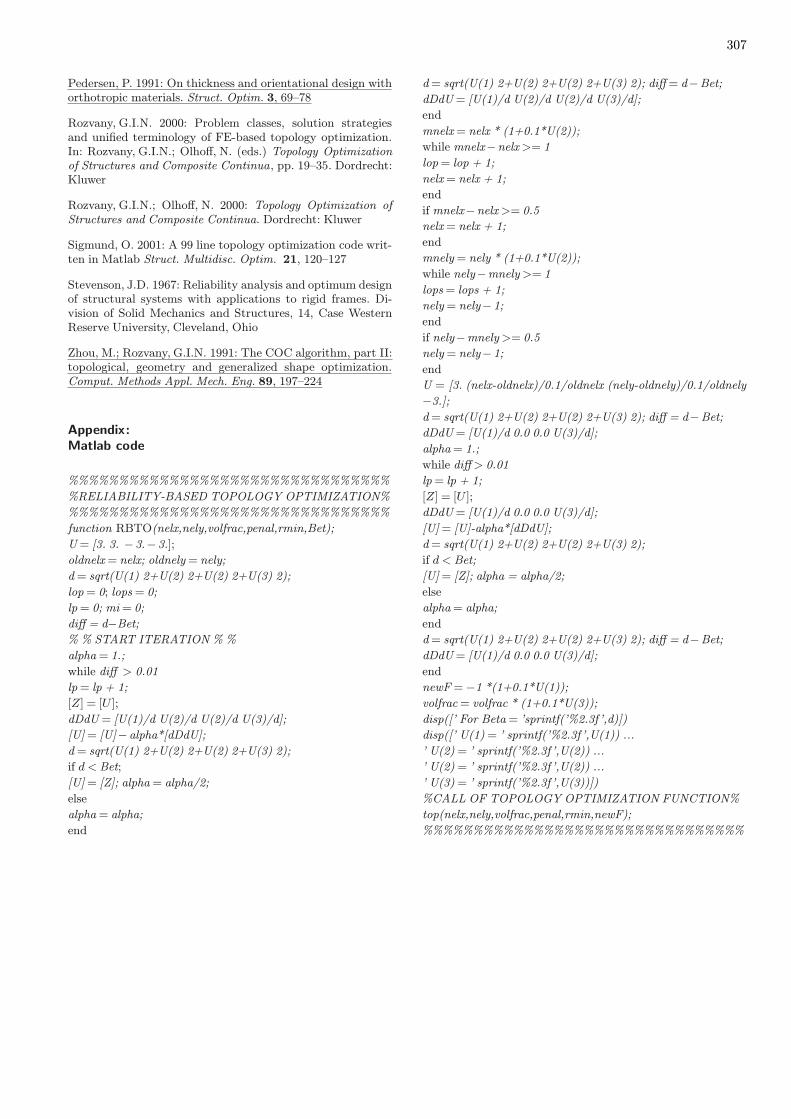
Appendix:Matlab code

%%%%%%%%%%%%%%%%%%%%%%%%%%%%%%%%

%RELIABILITY-BASED TOPOLOGY OPTIMIZATION%

%%%%%%%%%%%%%%%%%%%%%%%%%%%%%%%%

function RBTO(nelx,nely,volfrac,penal,rmin,Bet);

U= [3. 3. −3.−3.];

oldnelx= nelx; oldnely= nely;

d= sqrt(U(1) 2+U(2) 2+U(2) 2+U(3) 2);

lop= 0; lops= 0;

lp= 0; mi= 0;

diff = d−Bet;

% % START ITERATION % %

alpha= 1.;

while diff > 0.01

lp= lp + 1;

[Z] = [U ];

dDdU= [U(1)/d U(2)/d U(2)/d U(3)/d];

[U]= [U]−alpha*[dDdU];

d= sqrt(U(1) 2+U(2) 2+U(2) 2+U(3) 2);

if d <Bet;

[U]= [Z]; alpha= alpha/2;

else

alpha= alpha;

end

d= sqrt(U(1) 2+U(2) 2+U(2) 2+U(3) 2); diff= d−Bet;

dDdU= [U(1)/d U(2)/d U(2)/d U(3)/d];

end

mnelx= nelx * (1+0.1*U(2));

while mnelx−nelx>= 1

lop= lop + 1;

nelx= nelx + 1;

end

if mnelx−nelx>= 0.5nelx= nelx + 1;

end

mnely= nely * (1+0.1*U(2));

while nely−mnely>= 1

lops= lops + 1;

nely= nely−1;

end

if nely−mnely>= 0.5

nely= nely−1;

end

U = [3. (nelx-oldnelx)/0.1/oldnelx (nely-oldnely)/0.1/oldnely

−3.];

d= sqrt(U(1) 2+U(2) 2+U(2) 2+U(3) 2); diff = d−Bet;

dDdU= [U(1)/d 0.0 0.0 U(3)/d];

alpha= 1.;

while diff> 0.01

lp= lp + 1;

[Z] = [U ];

dDdU= [U(1)/d 0.0 0.0 U(3)/d];

[U]= [U]-alpha*[dDdU];

d= sqrt(U(1) 2+U(2) 2+U(2) 2+U(3) 2);

if d < Bet;

[U]= [Z]; alpha = alpha/2;

else

alpha= alpha;

end

d= sqrt(U(1) 2+U(2) 2+U(2) 2+U(3) 2); diff = d−Bet;

dDdU= [U(1)/d 0.0 0.0 U(3)/d];

end

newF=−1 *(1+0.1*U(1));

volfrac= volfrac * (1+0.1*U(3));

disp([’ For Beta= ’sprintf(’%2.3f ’,d)])

disp([’ U(1)= ’ sprintf(’%2.3f ’,U(1)) ...

’ U(2)= ’ sprintf(’%2.3f ’,U(2)) ...

’ U(2)= ’ sprintf(’%2.3f ’,U(2)) ...

’ U(3)= ’ sprintf(’%2.3f ’,U(3))])

%CALL OF TOPOLOGY OPTIMIZATION FUNCTION%

top(nelx,nely,volfrac,penal,rmin,newF);

%%%%%%%%%%%%%%%%%%%%%%%%%%%%%%%%