arX

iv:h

ep-p

h/01

0317

7v1

15

Mar

200

1

YITP-SB-01-10

Evolution program for parton densities withperturbative heavy flavor boundary conditions

A. Chuvakin, J. SmithC.N. Yang Institute for Theoretical Physics,

State University of New York at Stony Brook, New York 11794-3840.

February 2001

Abstract

A new code for the scale evolution of modified-minimal-subtraction-schemeparton densities is described. Through next-to-leading order the program usesexact splitting functions. In next-to-next-to-leading order approximate split-ting functions are used. For efficiency the program includes analytical resultsfor the evaluation of the weights required for the integrations over the lon-gitudinal momentum fractions of the partons. It also incorporates the opera-tor matrix elements required for the matching conditions across heavy flavorthresholds in higher order perturbation theory. The more efficient handling ofthe weights implies that the code is faster than similar evolution codes in allmodes of operation. The program is written in the C programming language.

PACS numbers: 11.10Jj, 12.38Bx, 13.60Hb, 13.87Ce.

1

Contents

1 Program Summary 3

2 Introduction 5

3 The evolution equations 8

3.1 Definitions of densities 8

3.2 The evolution equations 8

4 Direct x-space method of solution and initial conditions 12

4.1 The method 12

4.2 The initial conditions 15

4.3 The calculation of the running coupling 16

4.4 The evolution process 16

5 Input parameter description and usage 19

6 Description of the program 23

6.1 Program module summary 23

6.2 main.c 23

6.3 l-a-w.c 24

6.4 nl-a-w.c 24

6.5 alpha.c 25

6.6 init.c 25

6.7 polylo.c 25

6.8 intpol.c 26

6.9 evolver.c 26

6.10 thresh.c 26

6.11 a-coefs.c 27

6.12 loader.c 27

2

6.13 quadrat.c 28

6.14 daind.c 28

6.15 integrands.c 28

6.16 grids.c 29

6.17 weights.c 29

6.18 nnl-a-w.c 29

6.19 wgplg.c 30

7 Results 31

8 Error code descriptions 37

9 Conclusions 38

10 Acknowledgments 38

A Appendix A 39

B Appendix B 42

References 46

1 Program Summary

Title of Program: ADENSComputer: AlphaStation 4/500Operating system: OSF V3.2Programming language: CNumber of lines in distributed program: 11658Keywords: parton density, evolution, numerical solution, splitting function,next-to-next-to-leading orderNature of physical problem: solution of the parton density evolution equationswith LO, NLO and NNLO splitting functions and NLO, NNLO heavy flavorthreshold matching conditionsMethod of solution: x-space integration with analytic evaluation of weightsTypical running time: see table in Section 7The program www site:

http://insti.physics.sunysb.edu/∼chuvakin/adens-24.0.tar.gz

3

http://insti.physics.sunysb.edu/∼smith/adens-24.0.tar.gz

4

Contents

2 Introduction

Deep-inelastic lepton-hadron scattering experiments probe the internal struc-ture of hadrons. The lepton-hadron inclusive cross sections may be writtenin terms of structure functions, which depend on the virtuality of the probeQ2. Three structure functions F1, F2 and FL are necessary to describe neu-tral current (photon and Z-boson exchange) and charged current (W -bosonexchange) reactions. In perturbative quantum chromodynamics (pQCD) theprobe interacts with partonic constituents of the hadron. There are probabilitydensities f(x, µ2) to find partons carrying a fraction x (0 < x ≤ 1) of the lon-gitudinal momentum of the hadron at a mass factorization scale µ. Thereforethe Fi, i = 1, 2, L also depend on x and µ.

The operator product expansion (OPE) allows the structure functions to bewritten as convolutions of the parton (quark and gluon) probability densitieswith partonic hard scattering cross sections (or coefficient functions). The lat-ter can be calculated in pQCD. Even though the former cannot be calculated inpQCD, their µ dependence is determined by a set of integro-differential equa-tions, the (Dokshitzer-Gribov-Lipatov)-Altarelli-Parisi evolution equations [1],which follow from renormalization group analysis. Discussions of the pQCDdescription of deep inelastic scattering reactions are available in [2] and [3].The probability densities and splitting functions are defined in the modified-minimal-subtraction (MS) scheme.

For simplicity we will call the above equations the evolution equations. Theydescribe processes where a massless parton (quark or gluon) carrying a fractionof the longitudinal momentum of the incoming hadron radiates a masslessparton and becomes a (different) massless parton with a different momentumfraction. The probability for this process to happen is determined by splittingfunctions which are computed order-by-order in pQCD. The leading-order(LO) and next-to-leading order (NLO) splitting functions have been knownfor some time [4], [5], [6], [7], [8], [9] and the results are summarized in aconvenient form in [3]. Recently some moments of the next-to-next-to-leadingorder (NNLO) splitting functions have been calculated in [10], see also [11]and [12] . If the x-dependence of the quark and gluon densities in a hadron areparametrized at one value of µ, (say at µ0,) then the solutions of the evolutionequations with the above LO, NLO or NNLO splitting functions yield thex dependence of the massless parton densities at a different µ. There is asecond scale in the pQCD theory, the renormalization scale, which appears inargument of the the running coupling αs. It is usually set to be the same asthe mass factorization scale µ so αs = αs(µ

2).

5

The flavor dependence of the quark and anti-quark densities is governed bythe flavor group, which is SU(2) for the up and down quarks, SU(3) for theup, down and strange quarks etc. Therefore is is convenient to form flavornon-singlet and flavor (pure) singlet combinations of densities. The formerhave their own evolution equations. The latter mix with the gluons and thecombined evolution is described by matrices which obey coupled integro-differential equations.

A number of methods to solve the evolution equations for the parton densitieshave been proposed, including direct x-space methods, [13], [14], [15], [16], [17],[18], orthogonal polynomial methods [19], [20], and Mellin-transform methods[21], [22]. A compilation of parton density sets is available in [23].

The best method, which should be both accurate and fast, depends on regionchosen in x and µ2. Currently the requirements are that the code be able toevolve densities from a minimum µ2 near 0.26 GeV2 up to a maximum µ2 near106 GeV2 required for QCD studies for the future Large Hadron Collider atCERN. The range in x is from a minimum value near 10−5 up to a maximumnear unity. We use the direct x-space method, with the following additionalfeatures.

One of our aims is a better treatment of parton density evolution for ”light”u, d and s quarks near the heavy flavor thresholds chosen to be at the charmand the bottom quark masses (mc and mb respectively). The parton densitydescription must be modified to incorporate new c and b ”heavy” quark den-sities as the evolution scale increases. The implementation of the NLO andNNLO matching conditions across heavy flavor thresholds in the variable fla-vor number schemes (VFNS) [24], [25], [26], [27] involve large cancellationsbetween various terms in the expressions for the structure functions. Poor nu-merical accuracy in the solution for the evolution of the parton densities atsmall scales would spoil these cancellations and ruin the VFNS predictions.We achieve the required accuracy by avoiding one numerical integration inour program so we analytically calculate the weights for the exact LO, theexact NLO and the approximate NNLO splitting functions. The approximateNNLO splitting functions are taken from [28],[29], while the relevant opera-tor matrix elements (OMEs), which provide the matching conditions on theparton densities across heavy flavor thresholds, are taken from [30].

Since we start the scale evolution from a set of densities (input boundaryconditions) at a low scale µ = µ0 ≪ mc, the running coupling αs(µ

2) is large.We therefore use the exact solution of the NLO equation for αs and match thevalues on both sides of the heavy flavor thresholds to three decimal places. Wemention here that the NNLO matching conditions on αs across heavy flavorthresholds are available in [31] and [32]. Our program evolves both light andheavy parton densities in LO, NLO and NNLO from a minimum x equal to

6

10−7 to a maximum x equal to unity, a mimimum µ2 = 0.26 (GeV)2 in LOand µ2 = 0.40 (GeV)2 in NLO and NNLO and and a maximum µ2 = 106

(GeV)2. Results have been published in [25], [26], [27] and [33]. Here we givea detailed write up of the program.

7

3 The evolution equations

3.1 Definitions of densities

We evolve combinations of up (u), down (d), strange (s), charm (c) and bot-tom (b) quark densities which transform appropriately under the flavor group.Hence we define flavor-non-singlet valence quark densities by

fk−k(nf , x, µ2) ≡ fk(nf , x, µ2) − fk(nf , x, µ2) , k = u, d . (3.1)

The flavor-singlet quark densities

fSq (nf , x, µ2) =

nf∑

k=1

fk+k(nf , x, µ2) (3.2)

are defined in terms of the expression

fk+k(nf , x, µ2) ≡ fk(nf , x, µ2) + fk(nf , x, µ2) , k = u, d, s, c, b , (3.3)

when nf = 5. Then the flavor-non-singlet sea quark densities are

fNSq (nf , x, µ2) = fk+k(nf , x, µ2) − 1

nf

fSq (nf , x, µ2) . (3.4)

These equations will be discussed further in the next section.

3.2 The evolution equations

A typical evolution equation is that for a flavor-non-singlet parton densityfNS(x, µ2)

∂

∂ ln µ2fNS(y, µ2) =

αs(µ2)

2π

1∫

y

dx

xPNS(

y

x, µ2) fNS(x, µ2) , (3.5)

where P NS(y/x, µ2) is a non-singlet splitting function, and αs(µ2) is the run-

ning coupling.

8

The splitting functions in the evolution equations can be expanded in a per-turbation series in αs into LO, NLO and NNLO terms as follows

P (z, µ2) = P (0)(z, µ2) + (αs(µ

2)

2π)P (1)(z, µ2) + (

αs(µ2)

2π)2P (2)(z, µ2). (3.6)

The non-singlet combinations of the qr(qr) to qs(qs) splitting functions, wherethe subscripts r, s denote the flavors of the (anti)quarks q and q respectivelyand satisfy r, s = 1, · · · , nf , can be further decomposed into flavor diagonalparts proportional to δrs and flavor independent parts. In LO there is onlyone non-singlet splitting function Pqq but in NLO it is convenient to form twocombinations from Pqq and Pqq as follows

P+ = Pqq + Pqq ,

P− = Pqq − Pqq . (3.7)

These splitting functions are used to evolve two independent types of non-singlet densities, which will be called plus and minus respectively. They aregiven by

f+i = fNS

q (nf , x, µ2) ,

f−

j = fk−k(nf , x, µ2) . (3.8)

Since the general formulae in Eqs. (3.1)-(3.4) are rather involved the easiestway to explain the indices is by explicitly giving the combinations we use. Forj = 1, 2 we have

f−

1 = u − u , f−

2 = d − d , (3.9)

which are used for all flavor density sets. Then for three-flavor densities i =1, 2, 3 and we define

f+1 = u + u − Σ(3)/3 , f+

2 = d + d − Σ(3)/3 ,

f+3 = s + s − Σ(3)/3 , (3.10)

where Σ(3) = fSq (3) = u + u + d + d + s + s. These densities should be used

for scales µ < mc. For four-flavor densities i = 1, 2, 3, 4 and we define

f+1 = u + u − Σ(4)/4 , f+

2 = d + d − Σ(4)/4 ,

f+3 = s + s − Σ(4)/4 , f+

4 = c + c − Σ(4)/4 , (3.11)

where Σ(4) = fSq (4) = c + c + Σ(3). These should be used for scales in the

region mc ≤ µ < mb. For five-flavor densites i = 1, 2, 3, 4, 5 and we define

9

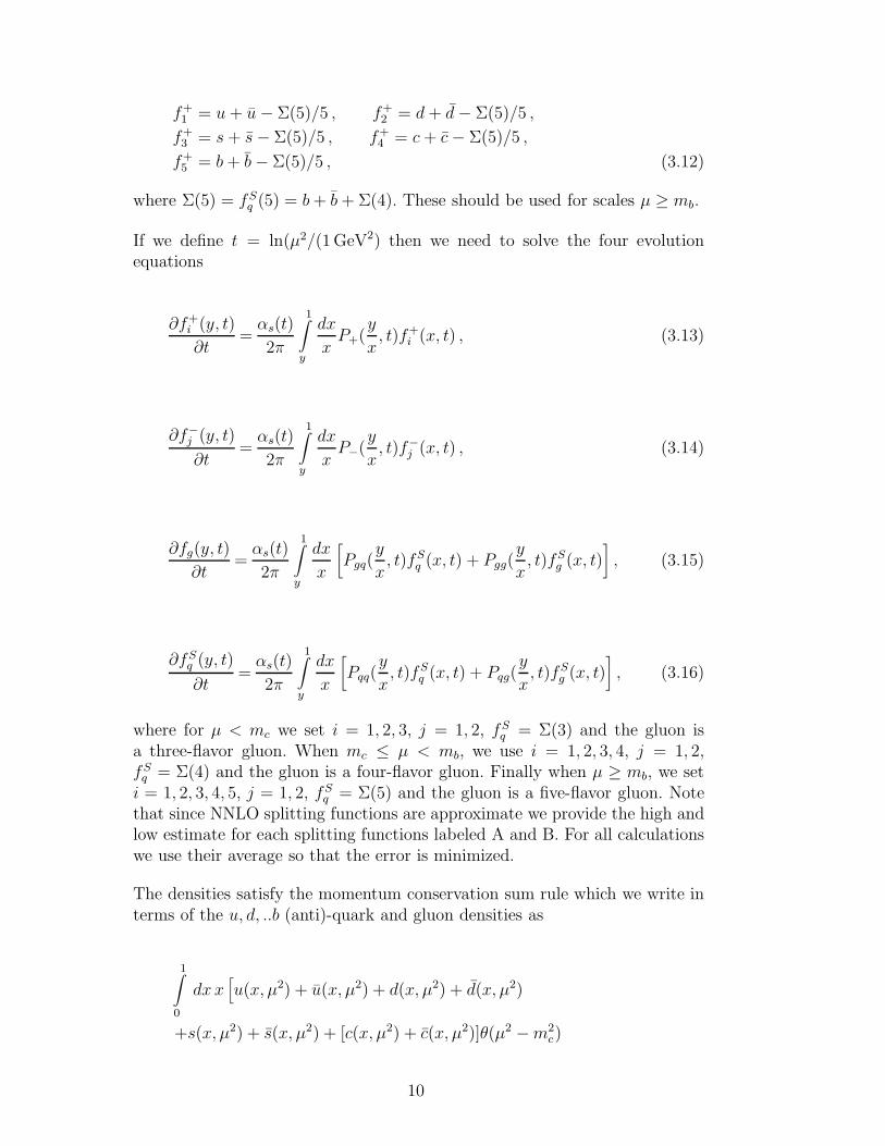
f+1 = u + u − Σ(5)/5 , f+

2 = d + d − Σ(5)/5 ,

f+3 = s + s − Σ(5)/5 , f+

4 = c + c − Σ(5)/5 ,

f+5 = b + b − Σ(5)/5 , (3.12)

where Σ(5) = fSq (5) = b + b + Σ(4). These should be used for scales µ ≥ mb.

If we define t = ln(µ2/(1 GeV2) then we need to solve the four evolutionequations

∂f+i (y, t)

∂t=

αs(t)

2π

1∫

y

dx

xP+(

y

x, t)f+

i (x, t) , (3.13)

∂f−

j (y, t)

∂t=

αs(t)

2π

1∫

y

dx

xP−(

y

x, t)f−

j (x, t) , (3.14)

∂fg(y, t)

∂t=

αs(t)

2π

1∫

y

dx

x

[

Pgq(y

x, t)fS

q (x, t) + Pgg(y

x, t)fS

g (x, t)]

, (3.15)

∂fSq (y, t)

∂t=

αs(t)

2π

1∫

y

dx

x

[

Pqq(y

x, t)fS

q (x, t) + Pqg(y

x, t)fS

g (x, t)]

, (3.16)

where for µ < mc we set i = 1, 2, 3, j = 1, 2, fSq = Σ(3) and the gluon is

a three-flavor gluon. When mc ≤ µ < mb, we use i = 1, 2, 3, 4, j = 1, 2,fS

q = Σ(4) and the gluon is a four-flavor gluon. Finally when µ ≥ mb, we seti = 1, 2, 3, 4, 5, j = 1, 2, fS

q = Σ(5) and the gluon is a five-flavor gluon. Notethat since NNLO splitting functions are approximate we provide the high andlow estimate for each splitting functions labeled A and B. For all calculationswe use their average so that the error is minimized.

The densities satisfy the momentum conservation sum rule which we write interms of the u, d, ..b (anti)-quark and gluon densities as

1∫

0

dx x[

u(x, µ2) + u(x, µ2) + d(x, µ2) + d(x, µ2)

+s(x, µ2) + s(x, µ2) + [c(x, µ2) + c(x, µ2)]θ(µ2 − m2c)

10

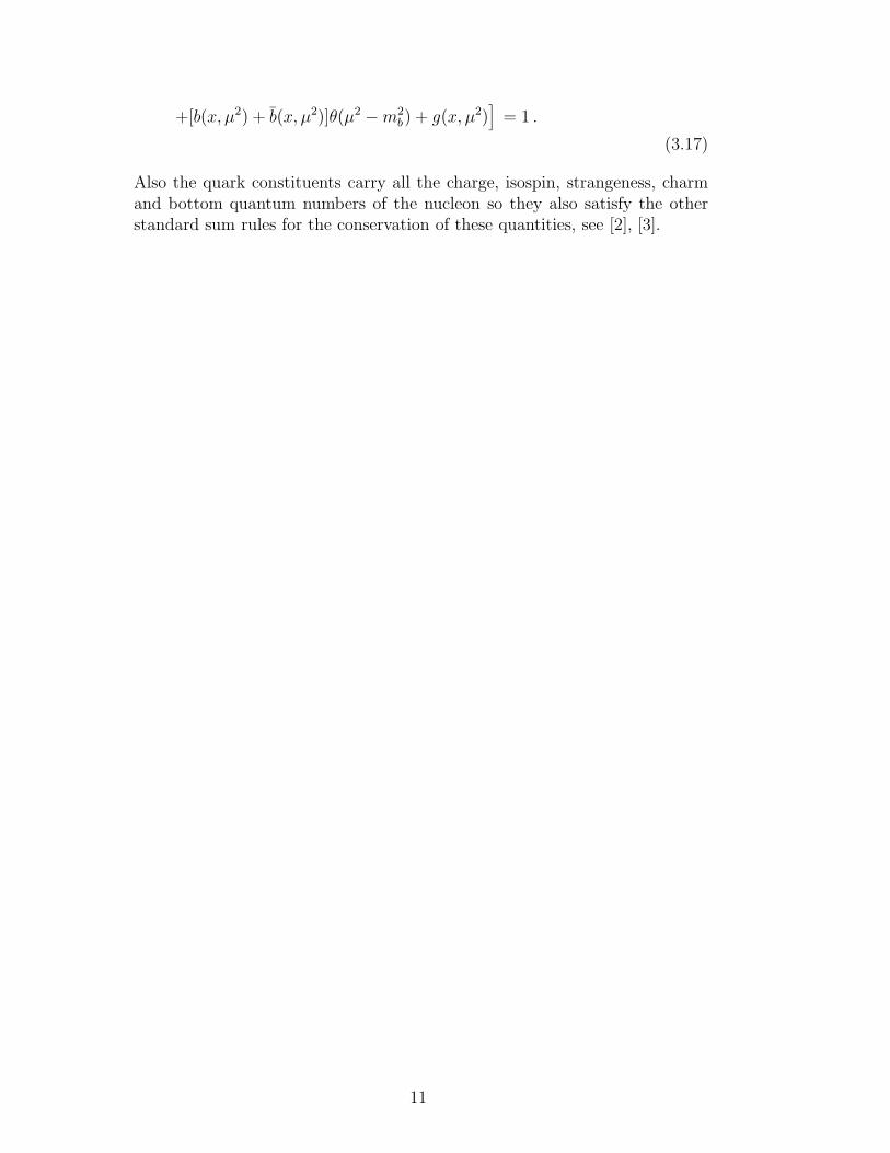
+[b(x, µ2) + b(x, µ2)]θ(µ2 − m2b) + g(x, µ2)

]

= 1 .

(3.17)

Also the quark constituents carry all the charge, isospin, strangeness, charmand bottom quantum numbers of the nucleon so they also satisfy the otherstandard sum rules for the conservation of these quantities, see [2], [3].

11

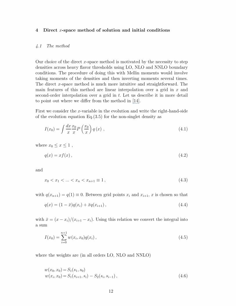
4 Direct x-space method of solution and initial conditions

4.1 The method

Our choice of the direct x-space method is motivated by the necessity to stepdensities across heavy flavor thresholds using LO, NLO and NNLO boundaryconditions. The procedure of doing this with Mellin moments would involvetaking moments of the densities and then inverting moments several times.The direct x-space method is much more intuitive and straightforward. Themain features of this method are linear interpolation over a grid in x andsecond-order interpolation over a grid in t. Let us describe it in more detailto point out where we differ from the method in [14].

First we consider the x-variable in the evolution and write the right-hand-sideof the evolution equation Eq.(3.5) for the non-singlet density as

I(x0) =∫

dx

x

x0

xP(

x0

x

)

q (x) , (4.1)

where x0 ≤ x ≤ 1 ,

q(x) = xf(x) , (4.2)

and

x0 < x1 < ... < xn < xn+1 ≡ 1 , (4.3)

with q(xn+1) = q(1) ≡ 0. Between grid points xi and xi+1, x is chosen so that

q(x) = (1 − x)q(xi) + xq(xi+1) , (4.4)

with x = (x− xi)/(xi+1 − xi). Using this relation we convert the integral intoa sum

I(x0) =n+1∑

i=0

w(xi, x0)q(xi) , (4.5)

where the weights are (in all orders LO, NLO and NNLO)

w(x0, x0)= S1(s1, s0)

w(xi, x0)= S1(si+1, si) − S2(si, si−1) , (4.6)

12

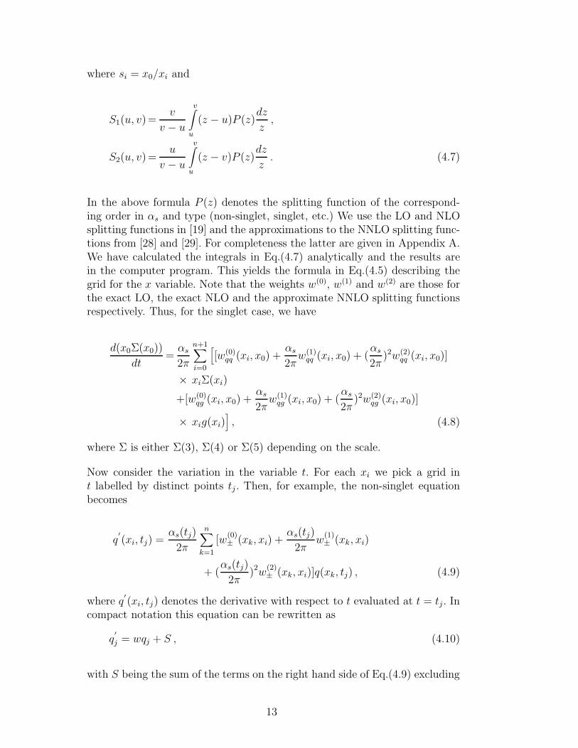
where si = x0/xi and

S1(u, v)=v

v − u

v∫

u

(z − u)P (z)dz

z,

S2(u, v)=u

v − u

v∫

u

(z − v)P (z)dz

z. (4.7)

In the above formula P (z) denotes the splitting function of the correspond-ing order in αs and type (non-singlet, singlet, etc.) We use the LO and NLOsplitting functions in [19] and the approximations to the NNLO splitting func-tions from [28] and [29]. For completeness the latter are given in Appendix A.We have calculated the integrals in Eq.(4.7) analytically and the results arein the computer program. This yields the formula in Eq.(4.5) describing thegrid for the x variable. Note that the weights w(0), w(1) and w(2) are those forthe exact LO, the exact NLO and the approximate NNLO splitting functionsrespectively. Thus, for the singlet case, we have

d(x0Σ(x0))

dt=

αs

2π

n+1∑

i=0

[

[w(0)qq (xi, x0) +

αs

2πw(1)

qq (xi, x0) + (αs

2π)2w(2)

qq (xi, x0)]

× xiΣ(xi)

+[w(0)qg (xi, x0) +

αs

2πw(1)

qg (xi, x0) + (αs

2π)2w(2)

qg (xi, x0)]

× xig(xi)]

, (4.8)

where Σ is either Σ(3), Σ(4) or Σ(5) depending on the scale.

Now consider the variation in the variable t. For each xi we pick a grid int labelled by distinct points tj . Then, for example, the non-singlet equationbecomes

q′

(xi, tj) =αs(tj)

2π

n∑

k=1

[w(0)± (xk, xi) +

αs(tj)

2πw

(1)± (xk, xi)

+ (αs(tj)

2π)2w

(2)± (xk, xi)]q(xk, tj) , (4.9)

where q′

(xi, tj) denotes the derivative with respect to t evaluated at t = tj . Incompact notation this equation can be rewritten as

q′

j = wqj + S , (4.10)

with S being the sum of the terms on the right hand side of Eq.(4.9) excluding

13

the j-th term.

For t between the grid points tj−1 and tj we interpolate the parton densityusing quadratic interpolation as follows:

q(xi, t) = at2 + bt + c . (4.11)

Thus we relate the value of q at the point tj to that of q at the point tj−1 by

q(xi, tj) = q(xi, tj−1) +1

2[q

′

(xi, tj) + q′

(xi, tj−1)]∆tj , (4.12)

where ∆tj = tj − tj−1. This equation can also be written more compactly as

qj = qj−1 +1

2(q

′

j−1 + q′

j)∆tj . (4.13)

The resulting system of two linear equations in Eq.(4.10) and Eq. (4.13) forqj and q

′

j has the solution

qj =2qj−1 + (q

′

j−1 + S)∆tj

2 − w∆tj. (4.14)

Then we find q′

j from Eq.(4.10). Applying the same procedure to the gluonand singlet combinations involves four equations because we have to computeboth the densities and their derivatives.

The evolution proceeds from the initial µ20 = µ2

LO (or µ20 = µ2

NLO) to the firstheavy flavor threshold at the scale µ2 = m2

c . Next the charm density is intro-duced in NNLO (α2

s-order terms) and all the four-flavor densities are evolvedfrom the new boundary conditions in Section 4.2. This evolution continuesup to the transition point µ2 = m2

b , where the same procedure is applied togenerate the bottom quark density. From that matching point all five-flavordensities are evolved up to all higher µ2 scales starting from the boundaryconditions in Appendix B.

Since the weights for the calculation are computed analytically from the LO,NLO [19] and NNLO ([28],[29]) MS splitting functions we remove possibleinstabilities in the numerical integrations. Hence the program is very efficientand fast. The results from the evolution code have been thoroughly checkedagainst the tables in the HERA report [16] and they agree to all five decimalplaces.

14

4.2 The initial conditions

The GRV98 [22] three-flavor LO and NLO parton density sets contain in-put formulae at low scales µ < mc which are ideal as initial values for ourparametrizations. Therefore we start our LO evolution using the followinginput at µ2

0 = µ2LO = 0.26 GeV2

xfu−u(3, x, µ20) =xuv(x, µ2

LO)

= 1.239 x0.48 (1 − x)2.72 (1 − 1.8√

x + 9.5x)

xfd−d(3, x, µ20) =xdv(x, µ2

LO)

= 0.614 (1 − x)0.9 xuv(x, µ2LO)

x(fd(3, x, µ20) − fu(3, x, µ2

0)) =x∆(x, µ2LO)

= 0.23 x0.48 (1 − x)11.3 (1 − 12.0√

x + 50.9x)

x(fd(3, x, µ20) + fu(3, x, µ2

0)) =x(u + d)(x, µ2LO)

= 1.52 x0.15 (1 − x)9.1 (1 − 3.6√

x + 7.8x)

xfg(3, x, µ20) =xg(x, µ2

LO)

= 17.47 x1.6 (1 − x)3.8

xfs(3, x, µ20) = xfs(3, x, µ2

0) =xs(x, µ2LO)

=xs(x, µ2LO) = 0 . (4.15)

Here ∆ ≡ d − u is used to construct the non-singlet combination.

We start the corresponding NLO evolution using the following GRV98 inputat µ2

0 = µ2NLO = 0.40 GeV2

xfu−u(3, x, µ20) =xuv(x, µ2

NLO)

= 0.632 x0.43 (1 − x)3.09 (1 + 18.2x)

xfd−d(3, x, µ20) =xdv(x, µ2

NLO)

= 0.624 (1 − x)1.0 xuv(x, µ2NLO)

x(fd(3, x, µ20) − fu(3, x, µ2

0)) =x∆(x, µ2NLO)

= 0.20 x0.43 (1 − x)12.4 (1 − 13.3√

x + 60.0x)

x(fd(3, x, µ20) + fu(3, x, µ2

0)) =x(u + d)(x, µ2NLO)

= 1.24 x0.20 (1 − x)8.5 (1 − 2.3√

x + 5.7x)

xfg(3, x, µ20) =xg(x, µ2

NLO)

= 20.80 x1.6 (1 − x)4.1

xfs(3, x, µ20) = xfs(3, x, µ2

0) =xs(x, µ2NLO)

=xs(x, µ2NLO) = 0. (4.16)

15

We start the corresponding NNLO evolution using the same NLO input andstarting scale as above.

4.3 The calculation of the running coupling

The heavy quark masses mc = 1.4 GeV2, mb = 4.5 GeV2 are used throughoutthe calculation. We also use the exact solution (as opposed to a perturbativesolution in inverse powers of ln(µ2/Λ2)) of the differential equation

d αs(µ2)

d ln(µ2)= −β0

4πα2

s(µ2) − β1

16π2α3

s(µ2) , (4.17)

for the running coupling αs(µ2). Here β0 = 11−2nf/3 and β1 = 102−38nf/3.

Another way of writing this equation is

lnµ2

(Λ(nf )EXACT)2

=4π

β0αs(µ2)− β1

β20

ln

[

4π

β0αs(µ2)+

β1

β20

]

. (4.18)

The values for Λ(nf )EXACT are carefully chosen to obtain accurate matching of αs

at the scales m2c and m2

b . We used the values Λ(3,4,5,6)EXACT = 299.4, 246, 167.7, 67.8

MeV/c2 respectively in the exact formula (which yields αEXACTs (m2

Z) = 0.114,αEXACT

s (m2b) = 0.205, αEXACT

s (m2c) = 0.319, αEXACT

s (µ2NLO) = 0.578 ) and

Λ(3,4,5,6)LO = 204, 175, 132, 66.5 MeV/c2 respectively (which yields αLO

s (m2Z)

= 0.125, αLOs (m2

b) = 0.232, αLOs (m2

c) = 0.362, αLOs (µ2

LO) = 0.763 ) for theLO formula (where β1 = 0). There is a NNLO discontinuity of aproximatelytwo parts in one thousand in the running coupling across heavy flavor thresh-olds [31], [32]. We have ignored this effect to focus on the numerically moresignificant matching of the flavor densities.

4.4 The evolution process

Three flavor evolution proceeds from the initial µ20 to the scale µ2 = m2

c = 1.96(GeV2)2. At this point the charm density is then defined by

fc+c(nf + 1, m2c) = a2

s(nf , m2c)[

APSQq(1) ⊗ fS

q (nf , m2c)

+ASQg(1) ⊗ fS

g (nf , m2c)]

, (4.19)

with nf = 3 and as = αs/4π. We have suppressed the x dependence to makethe notation more compact. The ⊗ symbol denotes the convolution integral

16

f ⊗ g =∫

f(x/y)g(y)dy/y, where x ≤ y ≤ 1. The OME’s APSQq(µ

2/m2c),

ASQg(µ

2/m2c) are given in [30] and are also listed in Appendix B. The rea-

son for choosing the matching scale µ at the mass of the charm quark mc isthat all the ln(µ2/m2

c) terms in the OME’s vanish at this point leaving onlythe nonlogarithmic pieces in the order α2

s OME’s to contribute to the right-hand-side of Eq.(4.19). Hence the LO and NLO charm densities vanish at thescale µ = mc. The NNLO charm density starts off with a finite x-dependentshape in order α2

s. Note that we then order the terms on the right-hand-sideof Eq. (4.19) so that it contains a product of NLO OME’s and LO partondensities. The result is then of order α2

s and should be multiplied by order α0s

coefficient functions when forming the deep inelastic structure functions.

The four-flavor gluon density is also generated at the matching point in thesame way. At µ = mc we define

fSg (nf + 1, m2

c) = fSg (nf , m

2c)

+a2s(nf , m

2c)[

ASgq,Q(1) ⊗ fS

q (nf , m2c) ,

+ASgg,Q(1) ⊗ fS

g (nf , m2c)]

. (4.20)

The OME’s ASgq,Q(µ2/m2

c), ASgg,Q(µ2/m2

c) are given in [30] and are also listedin the Appendix B. The four-flavor light quark (u,d,s) densities are generatedusing

fk+k(nf + 1, m2c) = fk+k(nf , m

2c)

+a2s(nf , m

2c)A

NSqq,Q(1) ⊗ fk+k(nf , m

2c) . (4.21)

The OME ANSqq,Q(µ2/m2

c) is given in [30] (as well as in Appendix B) and thetotal four-flavor singlet quark density folows from the sum of Eqs. (4.19) and(4.21). In Eqs. (4.20) and (4.21) we set nf = 3. The remarks after Eq. (4.19)are relevant here too.

Next the resulting four-flavor densities are evolved using the four-flavor weightsin either LO, NLO and NNLO up to the scale µ2 = m2

b = 20.25 (GeV2)2. Thebottom quark density is then generated at this point using

fb+b(nf + 1, m2b)= a2

s(nf , m2b)[

APSQq(1) ⊗ fS

q (nf , m2b)

+A(S)Qg(1) ⊗ fS

g (nf , m2b)]

, (4.22)

and the gluon and light quark densities (which now include charm) are gener-ated using Eqs.(4.19)-(4.21) with nf = 4 and replacing m2

c by m2b . Therefore

only the nonlogarithmic terms in the order a2s OME’s contribute to the match-

ing conditions on the bottom quark density. Then all the densities are evolved

17

up to higher µ2 as a five-flavor set with either LO, NLO and NNLO splittingfunctions. This is valid until µ = mt ≈ 175 GeV2 above which one shouldswitch to a six-flavor set. We do not implement this step because the topquark density would be extremely small.

The procedure outlined above generates a full set of parton densities (gluon,singlet, non-singlet light and heavy quark densities,) for any x and µ2 from thethree-flavor LO, NLO and NNLO inputs in Eqs.(4.15) and (4.16). Note thatwe have used µ2 for the factorization and renormalization scales in the abovediscussion. In the computer program we use the notation that Q2 denotesthese scales, since this is done in all the previous computer codes for theparton densities.

18

5 Input parameter description and usage

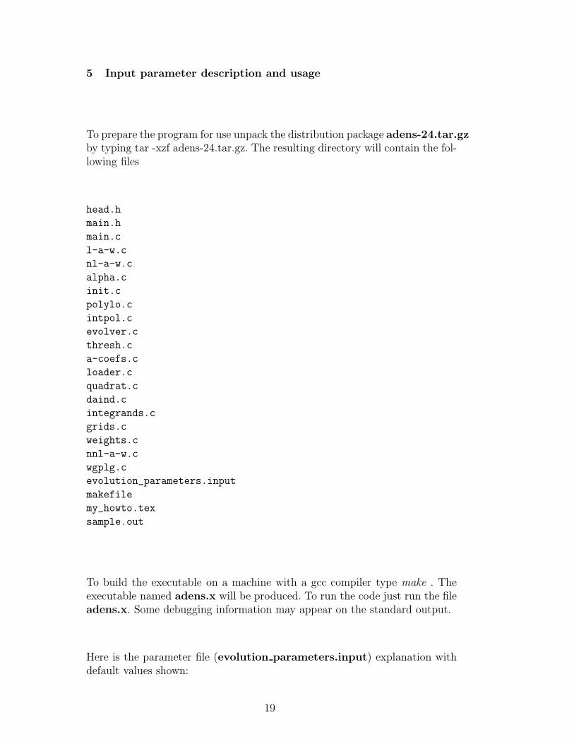
To prepare the program for use unpack the distribution package adens-24.tar.gz

by typing tar -xzf adens-24.tar.gz. The resulting directory will contain the fol-lowing files

head.h

main.h

main.c

l-a-w.c

nl-a-w.c

alpha.c

init.c

polylo.c

intpol.c

evolver.c

thresh.c

a-coefs.c

loader.c

quadrat.c

daind.c

integrands.c

grids.c

weights.c

nnl-a-w.c

wgplg.c

evolution_parameters.input

makefile

my_howto.tex

sample.out

To build the executable on a machine with a gcc compiler type make . Theexecutable named adens.x will be produced. To run the code just run the fileadens.x. Some debugging information may appear on the standard output.

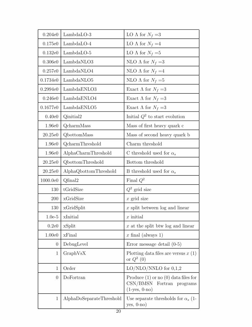
Here is the parameter file (evolution parameters.input) explanation withdefault values shown:

19

0.204e0 LambdaLO-3 LO Λ for Nf =3

0.175e0 LambdaLO-4 LO Λ for Nf =4

0.132e0 LambdaLO-5 LO Λ for Nf =5

0.306e0 LambdaNLO3 NLO Λ for Nf =3

0.257e0 LambdaNLO4 NLO Λ for Nf =4

0.1734e0 LambdaNLO5 NLO Λ for Nf =5

0.2994e0 LambdaENLO3 Exact Λ for Nf =3

0.246e0 LambdaENLO4 Exact Λ for Nf =3

0.1677e0 LambdaENLO5 Exact Λ for Nf =3

0.40e0 Qinitial2 Initial Q2 to start evolution

1.96e0 QcharmMass Mass of first heavy quark c

20.25e0 QbottomMass Mass of second heavy quark b

1.96e0 QcharmThreshold Charm threshold

1.96e0 AlphaCharmThreshold C threshold used for αs

20.25e0 QbottomThreshold Bottom threshold

20.25e0 AlphaQbottomThreshold B threshold used for αs

1000.0e0 Qfinal2 Final Q2

130 tGridSize Q2 grid size

200 xGridSize x grid size

130 xGridSplit x split between log and linear

1.0e-5 xInitial x initial

0.2e0 xSplit x at the split btw log and linear

1.00e0 xFinal x final (always 1)

0 DebugLevel Error message detail (0-5)

1 GraphVsX Plotting data files are versus x (1)or Q2 (0)

1 Order LO/NLO/NNLO for 0,1,2

0 DoFortran Produce (1) or no (0) data files forCSN/BMSN Fortran programs(1-yes, 0-no)

1 AlphaDoSeparateThreshold Use separate thresholds for αs (1-yes, 0-no)

20

1 AlphaUseExact Use exact GRV98-style αs (1-yes,0-no)

0 ThreeFlavorMode Calculate GRV98-style densitieswith no heavy flavors (1-yes, 0-no)

0 GraphAll Plot all data points (1-yes, 0-no)

0 NNLOmultiOrderCHARM Use our proper order NNLOheavy flavors (1-yes, 0-no)

1 DoBottomThreshold Generate bottom (1-yes, 0-no)

0 LoadWeightsMadeBefore Use ready weights if available (1-yes, 0-no)

1 DoNotDumpWeights Dump weight for future use as theoption above (1-yes, 0-no)

0 NLO4NNLO Use NLO weights for NNLO cal-culation (1-yes, 0-no)

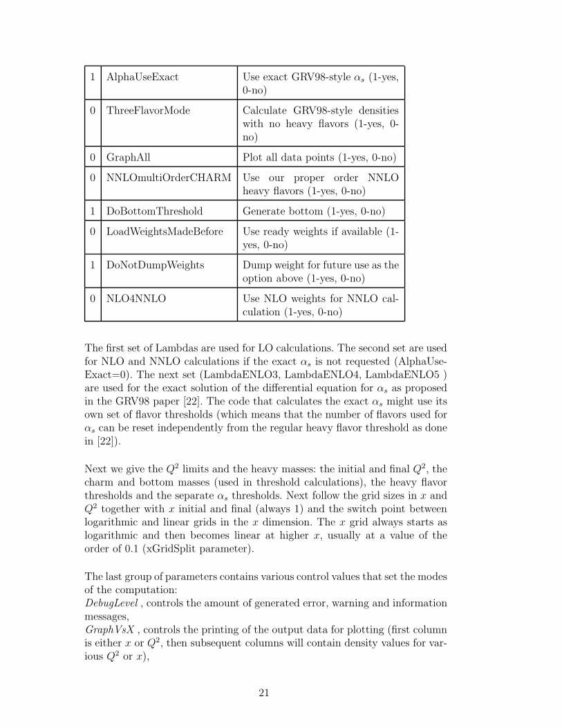
The first set of Lambdas are used for LO calculations. The second set are usedfor NLO and NNLO calculations if the exact αs is not requested (AlphaUse-Exact=0). The next set (LambdaENLO3, LambdaENLO4, LambdaENLO5 )are used for the exact solution of the differential equation for αs as proposedin the GRV98 paper [22]. The code that calculates the exact αs might use itsown set of flavor thresholds (which means that the number of flavors used forαs can be reset independently from the regular heavy flavor threshold as donein [22]).

Next we give the Q2 limits and the heavy masses: the initial and final Q2, thecharm and bottom masses (used in threshold calculations), the heavy flavorthresholds and the separate αs thresholds. Next follow the grid sizes in x andQ2 together with x initial and final (always 1) and the switch point betweenlogarithmic and linear grids in the x dimension. The x grid always starts aslogarithmic and then becomes linear at higher x, usually at a value of theorder of 0.1 (xGridSplit parameter).

The last group of parameters contains various control values that set the modesof the computation:DebugLevel , controls the amount of generated error, warning and informationmessages,GraphVsX , controls the printing of the output data for plotting (first columnis either x or Q2, then subsequent columns will contain density values for var-ious Q2 or x),

21

Order, sets calculation order (use 0,1,2 for LO,NLO,NNLO),DoFortran, sets whether to dump interpolated densities on a special grid forfuture use in Fortran code for the calculation of structure functions ; CSN andBMSN refer to VFNS schemes which are explained in [25],AlphaDoSeparateThreshold, sets whether we use a separate threshold for αs

(used, for instance for GRV98 set where nf for densities is always 3 and nf

for αs goes from 3 to 5,AlphaUseExact, sets whether to use exact (differential equation solution) αs

for NLO and NNLO calculation,ThreeFlavorMode, sets whether to run GRV98 mode (no heavy flavors, nf = 3for all Q2),GraphAll, controls the amount of graphing and printing output (either all datapoints or the special grid defined in the file main.h, that contains some fa-vorite values (for more see Section 7)),NNLOmultiOrderCHARM, activates NNLO threshold calculation using properorder combinations (this mode requires one to first run the LO and NLO cal-culations),DoBottomThreshold, enables the bottom density,LoadWeightsMadeBefore, turns on and off the loading of weights computed inthe prior runs,DoNotDumpWeights, sets whether to save computed weights to disk for futureuse,NLO4NNLO, sets whether NLO weights are used for the NNLO calculation(thus having only the boundary condition in NNLO).

Some common parameter settings and typical grid sizes for popular evolutionsare shown in Section 7.

22

6 Description of the program

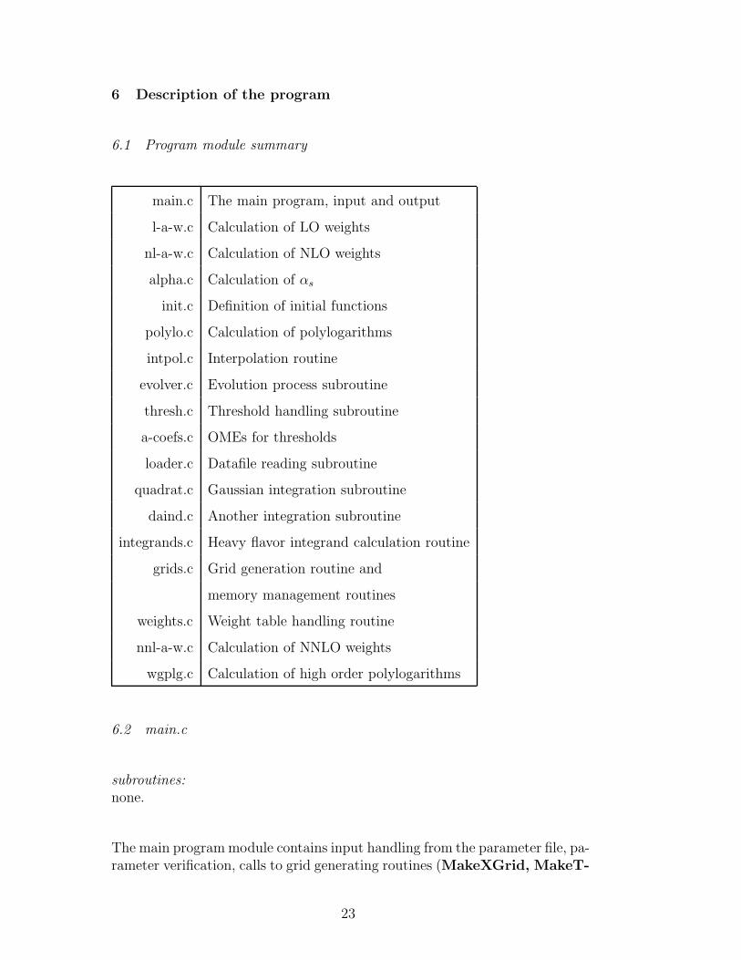
6.1 Program module summary

main.c The main program, input and output

l-a-w.c Calculation of LO weights

nl-a-w.c Calculation of NLO weights

alpha.c Calculation of αs

init.c Definition of initial functions

polylo.c Calculation of polylogarithms

intpol.c Interpolation routine

evolver.c Evolution process subroutine

thresh.c Threshold handling subroutine

a-coefs.c OMEs for thresholds

loader.c Datafile reading subroutine

quadrat.c Gaussian integration subroutine

daind.c Another integration subroutine

integrands.c Heavy flavor integrand calculation routine

grids.c Grid generation routine and

memory management routines

weights.c Weight table handling routine

nnl-a-w.c Calculation of NNLO weights

wgplg.c Calculation of high order polylogarithms

6.2 main.c

subroutines:

none.

The main program module contains input handling from the parameter file, pa-rameter verification, calls to grid generating routines (MakeXGrid, MakeT-

23

Grid), resets for all density arrays (array q) and their derivatives (array qp).It also includes calls to the generation of weights (analowgts, ananlowgts

), the calls to evolution and threshold routines (evolver, threshold) that dothe actual work. Also it contains some pre-output density processing and theresults provided in various formats for both viewing and plotting.

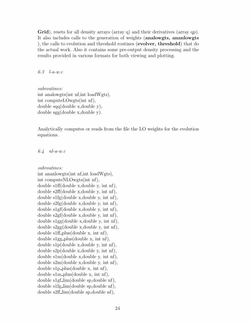
6.3 l-a-w.c

subroutines:

int analowgts(int nf,int loadWgts),int computeLOwgts(int nf),double sqq(double x,double y),double sgg(double x,double y).

Analytically computes or reads from the file the LO weights for the evolutionequations.

6.4 nl-a-w.c

subroutines:

int ananlowgts(int nf,int loadWgts),int computeNLOwgts(int nf),double s1ff(double x,double y, int nf),double s2ff(double x,double y, int nf),double s1fg(double x,double y, int nf),double s2fg(double x,double y, int nf),double s1gf(double x,double y, int nf),double s2gf(double x,double y, int nf),double s1gg(double x,double y, int nf),double s2gg(double x,double y, int nf),double s1ff plus(double x, int nf),double s1gg plus(double x, int nf),double s1p(double x,double y, int nf),double s2p(double x,double y, int nf),double s1m(double x,double y, int nf),double s2m(double x,double y, int nf),double s1p plus(double x, int nf),double s1m plus(double x, int nf),double s1gf lim(double sp,double nf),double s1fg lim(double sp,double nf),double s2ff lim(double sp,double nf),

24

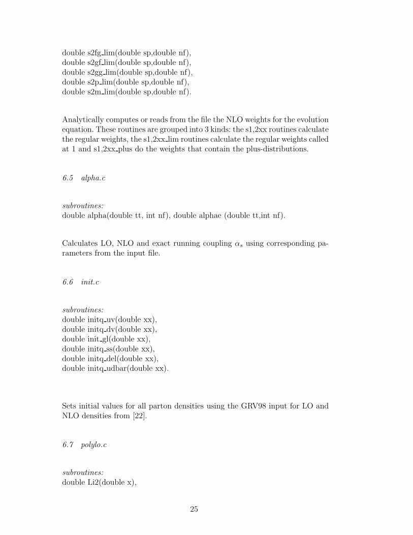
double s2fg lim(double sp,double nf),double s2gf lim(double sp,double nf),double s2gg lim(double sp,double nf),double s2p lim(double sp,double nf),double s2m lim(double sp,double nf).

Analytically computes or reads from the file the NLO weights for the evolutionequation. These routines are grouped into 3 kinds: the s1,2xx routines calculatethe regular weights, the s1,2xx lim routines calculate the regular weights calledat 1 and s1,2xx plus do the weights that contain the plus-distributions.

6.5 alpha.c

subroutines:

double alpha(double tt, int nf), double alphae (double tt,int nf).

Calculates LO, NLO and exact running coupling αs using corresponding pa-rameters from the input file.

6.6 init.c

subroutines:

double initq uv(double xx),double initq dv(double xx),double init gl(double xx),double initq ss(double xx),double initq del(double xx),double initq udbar(double xx).

Sets initial values for all parton densities using the GRV98 input for LO andNLO densities from [22].

6.7 polylo.c

subroutines:

double Li2(double x),

25

double Li3(double x),double S12(double x).

Calculates these three polylogarithms using a fast routine with Bernouilli num-bers. .

6.8 intpol.c

subroutines:

double int q(int j,double xx,int it),double interpolate(double xx,double *xt, double *yt,int points).

Interpolation routines used to calculate densities between grid points and forintegration at the threshold.

6.9 evolver.c

subroutines:

evolver(int it1,int it2,int ic,int ib).

The main routine that performs the evolution between thresholds for all den-sities. It updates the main density array q and the density derivatives arrayqp.

6.10 thresh.c

subroutines:

int threshold(int what,int itt),int fdens4(double xx,int ittc,double *u,double *d,double *s),double light charm(double xx,int ittc),double fcharm(double xx,int ittc),double fbottom(double xx,int ittc),double fsigma(double xx,int ittc),double fgluon(double xx,int ittc),double fcharm(double xx,int ittc),double fbottom(double xx,int ittc).

26

Threshold handling routines to implement LO, NLO and NNLO matching con-ditions for light and heavy densities at the charm and bottom thresholds. Thedensity routines are calls to convolution integrals that generate new densitiesfor nf + 1 flavors.

6.11 a-coefs.c

subroutines:

double a1qg(double z,double fs2,double hm2),double a2qq(double z,double fs2,double hm2),double a2qg(double z,double fs2,double hm2),double a2qqns(double z,double fs2,double hm2),double softq(double z,double fs2,double hm2),double corq(double z,double fs2,double hm2),double a2gg(double z,double fs2,double hm2),double softg(double z,double fs2,double hm2),double corg1(double fs2,double hm2),double corg2(double z,double fs2,double hm2),double a2gq(double z,double fs2,double hm2).

The OME routines used for NNLO threshold matching. These contain theformulae in Appendix B.

6.12 loader.c

subroutines:

int loadOrd(int what).

Functions to handle threshold datafile loading, saving and verification. Thisfile allows one the ability to use previously computed density values at thethreshold in a new computation.

27

6.13 quadrat.c

subroutines:

double qadrat(double *x, double a, double b, double (*fx)(double), double e[]),double lint(double *x, double (*fx)(double), double e[], double x0, double xn,double f0, double f2, double f3, double f5, double f6, double f7, double f9,double f14, double hmin, double hmax, double re, double ae).

Backup integration routine used as a check for the actual one used in thethreshold integration.

6.14 daind.c

subroutines:

double daind(double *x,double a,double b, double (*fun)(double),double eps,intkey,int max).

Main Gaussian integration routine, see [34].

6.15 integrands.c

subroutines:

inline double fcharm integrand(double x1),inline double fgluon integrand(double x1),inline double fsigma integrand(double x1),inline double us integrand(double x1),inline double ds integrand(double x1),inline double ss integrand(double x1),inline double fbottom integrand(double x1),inline double light charm integrand(double x1).

Functions containing integrands for the threshold integration. They use thedensity values and the coefficient functions from a-coefs.c to produce the in-tegrands that are then fed into the Gaussian integration program.

28

6.16 grids.c

subroutines:

int MakeXGrid(void),int MakeTGrid(void),int merge(double *a,double *b,int na, int nb,char w),int check grid(double *a,int n,char w),int MakeFortranGrid(int test mode),double **allocate real matrix(int ur, int uc),void free real matrix(double **m,int ur).

Subroutines for making (and also merging and verifying) the initial grids inx and Q2 and the final grids for Fortran-code compatible output. The gridmerging is used to combine the evenly spaced grid generated automaticallyfrom the initial and final values with the premade grid containing several xand Q2 values for plotting and outputting the data. Two routines are addedfor deallocating memory.

6.17 weights.c

subroutines:

int readWeights(int nf,int order),int dumpWeights(int nf,int order).

Routines dealing with loading and saving computed NLO and NNLO weighttables to do a fast calculation on the same grids. LO weights are not saved asit is very fast to compute them every time.

6.18 nnl-a-w.c

subroutines:

int anannlowgts(int nf,int loadWgts),int computeNNLOwgts(int nf),double nn s1ff(double x,double y, int nf),double nn s2ff(double x,double y, int nf),double nn s1fg(double x,double y, int nf),double nn s2fg(double x,double y, int nf),double nn s1gf(double x,double y, int nf),

29

double nn s2gf(double x,double y, int nf),double nn s1gg(double x,double y, int nf),double nn s2gg(double x,double y, int nf),double nn s1ff plus(double x, int nf),double nn s1gg plus(double x, int nf),double nn s1p(double x,double y, int nf),double nn s2p(double x,double y, int nf),double nn s1m(double x,double y, int nf),double nn s2m(double x,double y, int nf),double nn s1p plus(double x, int nf),double nn s1m plus(double x, int nf),double nn s1gf lim(double sp,double nf),double nn s1fg lim(double sp,double nf),double nn s2ff lim(double sp,double nf),double nn s2fg lim(double sp,double nf),double nn s2gf lim(double sp,double nf),double nn s2gg lim(double sp,double nf),double nn s2p lim(double sp,double nf),double nn s2m lim(double sp,double nf).

Analytically computes or reads from files the approximate NNLO weights forthe evolution equations. Here the routines are grouped into three kinds: thenn s1,2xx routines calculate the regular weights, the nn s1,2xx lim routinescalculate the regular weights called at 1 and nn s1,2xx plus do the weightsthat contain the plus-distributions.

6.19 wgplg.c

subroutines:

double wgplg(int n,int p,double x).

The routines which calculate polylogarithms using the method from CERN-LIB [35]. They are only used for the higher order polylogarithms because theroutines for Li2, Li3 and S12 in polylo.c are faster.

30

7 Results

The code can be used in several modes of operation.

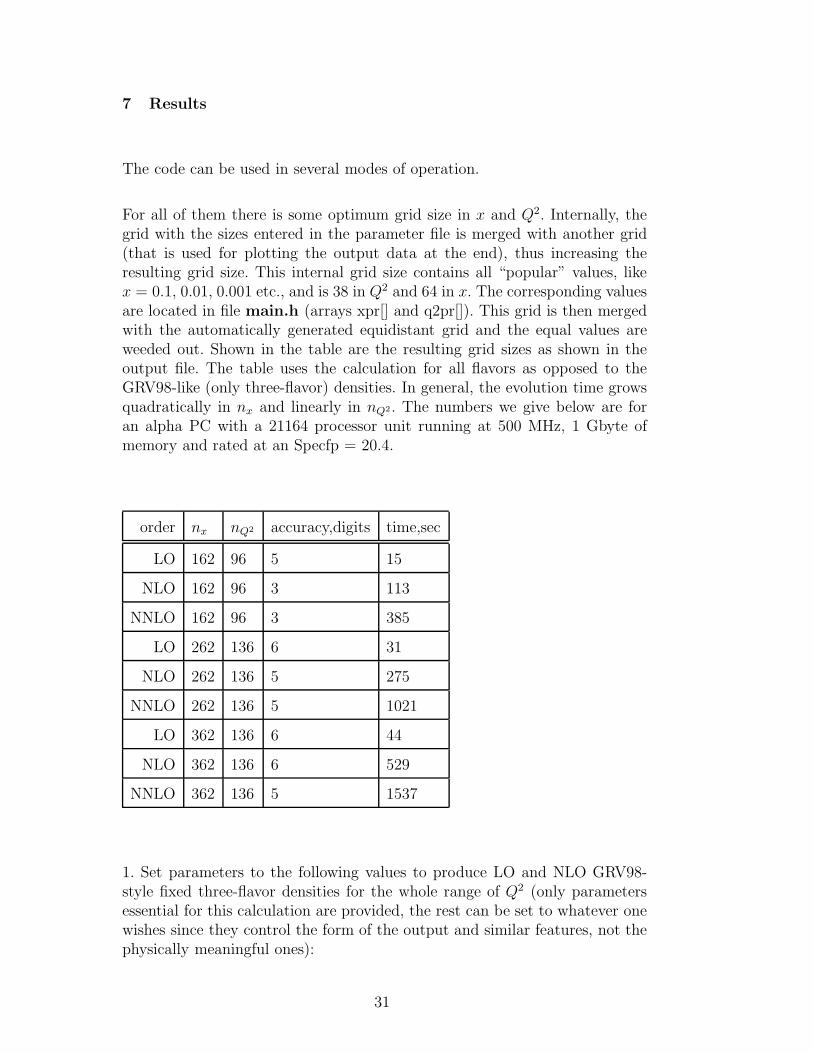
For all of them there is some optimum grid size in x and Q2. Internally, thegrid with the sizes entered in the parameter file is merged with another grid(that is used for plotting the output data at the end), thus increasing theresulting grid size. This internal grid size contains all “popular” values, likex = 0.1, 0.01, 0.001 etc., and is 38 in Q2 and 64 in x. The corresponding valuesare located in file main.h (arrays xpr[] and q2pr[]). This grid is then mergedwith the automatically generated equidistant grid and the equal values areweeded out. Shown in the table are the resulting grid sizes as shown in theoutput file. The table uses the calculation for all flavors as opposed to theGRV98-like (only three-flavor) densities. In general, the evolution time growsquadratically in nx and linearly in nQ2. The numbers we give below are foran alpha PC with a 21164 processor unit running at 500 MHz, 1 Gbyte ofmemory and rated at an Specfp = 20.4.

order nx nQ2 accuracy,digits time,sec

LO 162 96 5 15

NLO 162 96 3 113

NNLO 162 96 3 385

LO 262 136 6 31

NLO 262 136 5 275

NNLO 262 136 5 1021

LO 362 136 6 44

NLO 362 136 6 529

NNLO 362 136 5 1537

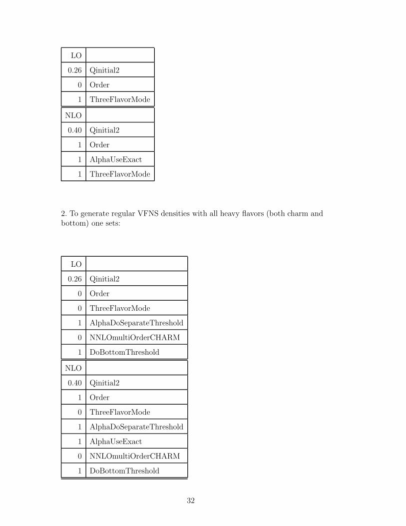
1. Set parameters to the following values to produce LO and NLO GRV98-style fixed three-flavor densities for the whole range of Q2 (only parametersessential for this calculation are provided, the rest can be set to whatever onewishes since they control the form of the output and similar features, not thephysically meaningful ones):

31

LO

0.26 Qinitial2

0 Order

1 ThreeFlavorMode

NLO

0.40 Qinitial2

1 Order

1 AlphaUseExact

1 ThreeFlavorMode

2. To generate regular VFNS densities with all heavy flavors (both charm andbottom) one sets:

LO

0.26 Qinitial2

0 Order

0 ThreeFlavorMode

1 AlphaDoSeparateThreshold

0 NNLOmultiOrderCHARM

1 DoBottomThreshold

NLO

0.40 Qinitial2

1 Order

0 ThreeFlavorMode

1 AlphaDoSeparateThreshold

1 AlphaUseExact

0 NNLOmultiOrderCHARM

1 DoBottomThreshold

32

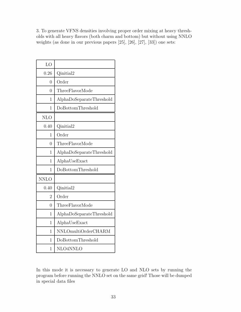
3. To generate VFNS densities involving proper order mixing at heavy thresh-olds with all heavy flavors (both charm and bottom) but without using NNLOweights (as done in our previous papers [25], [26], [27], [33]) one sets:

LO

0.26 Qinitial2

0 Order

0 ThreeFlavorMode

1 AlphaDoSeparateThreshold

1 DoBottomThreshold

NLO

0.40 Qinitial2

1 Order

0 ThreeFlavorMode

1 AlphaDoSeparateThreshold

1 AlphaUseExact

1 DoBottomThreshold

NNLO

0.40 Qinitial2

2 Order

0 ThreeFlavorMode

1 AlphaDoSeparateThreshold

1 AlphaUseExact

1 NNLOmultiOrderCHARM

1 DoBottomThreshold

1 NLO4NNLO

In this mode it is necessary to generate LO and NLO sets by running theprogram before running the NNLO set on the same grid! Those will be dumpedin special data files

33

(agrv99lo.BO.threshold, agrv99lo.CH.threshold,agrv99nlo.BO.threshold, and agrv99nlo.CH.threshold)that will later be read for the NNLO calculation wheneverNNLOmultiOrderCHARM=1.

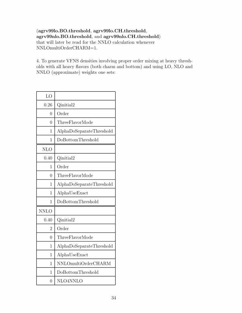
4. To generate VFNS densities involving proper order mixing at heavy thresh-olds with all heavy flavors (both charm and bottom) and using LO, NLO andNNLO (approximate) weights one sets:

LO

0.26 Qinitial2

0 Order

0 ThreeFlavorMode

1 AlphaDoSeparateThreshold

1 DoBottomThreshold

NLO

0.40 Qinitial2

1 Order

0 ThreeFlavorMode

1 AlphaDoSeparateThreshold

1 AlphaUseExact

1 DoBottomThreshold

NNLO

0.40 Qinitial2

2 Order

0 ThreeFlavorMode

1 AlphaDoSeparateThreshold

1 AlphaUseExact

1 NNLOmultiOrderCHARM

1 DoBottomThreshold

0 NLO4NNLO

34

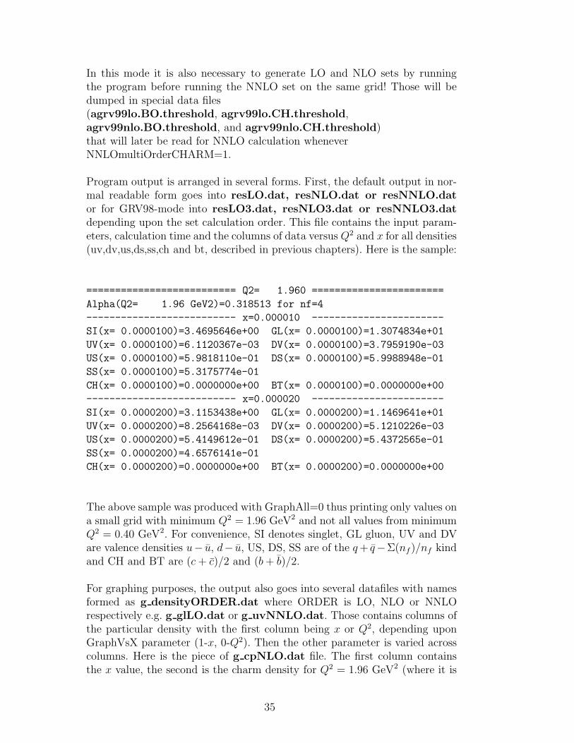
In this mode it is also necessary to generate LO and NLO sets by runningthe program before running the NNLO set on the same grid! Those will bedumped in special data files(agrv99lo.BO.threshold, agrv99lo.CH.threshold,agrv99nlo.BO.threshold, and agrv99nlo.CH.threshold)that will later be read for NNLO calculation wheneverNNLOmultiOrderCHARM=1.

Program output is arranged in several forms. First, the default output in nor-mal readable form goes into resLO.dat, resNLO.dat or resNNLO.dat

or for GRV98-mode into resLO3.dat, resNLO3.dat or resNNLO3.dat

depending upon the set calculation order. This file contains the input param-eters, calculation time and the columns of data versus Q2 and x for all densities(uv,dv,us,ds,ss,ch and bt, described in previous chapters). Here is the sample:

========================== Q2= 1.960 =======================

Alpha(Q2= 1.96 GeV2)=0.318513 for nf=4

-------------------------- x=0.000010 -----------------------

SI(x= 0.0000100)=3.4695646e+00 GL(x= 0.0000100)=1.3074834e+01

UV(x= 0.0000100)=6.1120367e-03 DV(x= 0.0000100)=3.7959190e-03

US(x= 0.0000100)=5.9818110e-01 DS(x= 0.0000100)=5.9988948e-01

SS(x= 0.0000100)=5.3175774e-01

CH(x= 0.0000100)=0.0000000e+00 BT(x= 0.0000100)=0.0000000e+00

-------------------------- x=0.000020 -----------------------

SI(x= 0.0000200)=3.1153438e+00 GL(x= 0.0000200)=1.1469641e+01

UV(x= 0.0000200)=8.2564168e-03 DV(x= 0.0000200)=5.1210226e-03

US(x= 0.0000200)=5.4149612e-01 DS(x= 0.0000200)=5.4372565e-01

SS(x= 0.0000200)=4.6576141e-01

CH(x= 0.0000200)=0.0000000e+00 BT(x= 0.0000200)=0.0000000e+00

The above sample was produced with GraphAll=0 thus printing only values ona small grid with minimum Q2 = 1.96 GeV2 and not all values from minimumQ2 = 0.40 GeV2. For convenience, SI denotes singlet, GL gluon, UV and DVare valence densities u− u, d− u, US, DS, SS are of the q + q−Σ(nf )/nf kindand CH and BT are (c + c)/2 and (b + b)/2.

For graphing purposes, the output also goes into several datafiles with namesformed as g densityORDER.dat where ORDER is LO, NLO or NNLOrespectively e.g. g glLO.dat or g uvNNLO.dat. Those contains columns ofthe particular density with the first column being x or Q2, depending uponGraphVsX parameter (1-x, 0-Q2). Then the other parameter is varied acrosscolumns. Here is the piece of g cpNLO.dat file. The first column containsthe x value, the second is the charm density for Q2 = 1.96 GeV2 (where it is

35

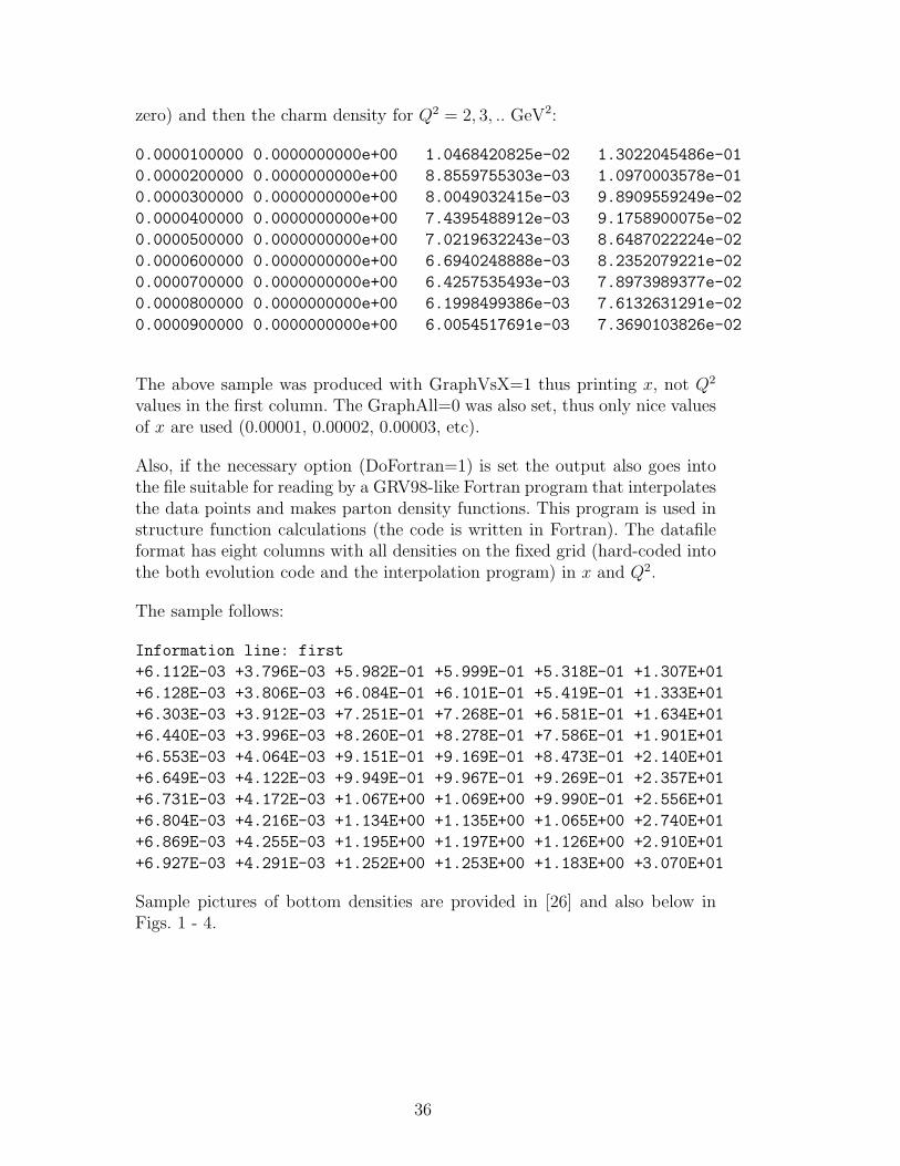
zero) and then the charm density for Q2 = 2, 3, .. GeV2:

0.0000100000 0.0000000000e+00 1.0468420825e-02 1.3022045486e-01

0.0000200000 0.0000000000e+00 8.8559755303e-03 1.0970003578e-01

0.0000300000 0.0000000000e+00 8.0049032415e-03 9.8909559249e-02

0.0000400000 0.0000000000e+00 7.4395488912e-03 9.1758900075e-02

0.0000500000 0.0000000000e+00 7.0219632243e-03 8.6487022224e-02

0.0000600000 0.0000000000e+00 6.6940248888e-03 8.2352079221e-02

0.0000700000 0.0000000000e+00 6.4257535493e-03 7.8973989377e-02

0.0000800000 0.0000000000e+00 6.1998499386e-03 7.6132631291e-02

0.0000900000 0.0000000000e+00 6.0054517691e-03 7.3690103826e-02

The above sample was produced with GraphVsX=1 thus printing x, not Q2

values in the first column. The GraphAll=0 was also set, thus only nice valuesof x are used (0.00001, 0.00002, 0.00003, etc).

Also, if the necessary option (DoFortran=1) is set the output also goes intothe file suitable for reading by a GRV98-like Fortran program that interpolatesthe data points and makes parton density functions. This program is used instructure function calculations (the code is written in Fortran). The datafileformat has eight columns with all densities on the fixed grid (hard-coded intothe both evolution code and the interpolation program) in x and Q2.

The sample follows:

Information line: first

+6.112E-03 +3.796E-03 +5.982E-01 +5.999E-01 +5.318E-01 +1.307E+01

+6.128E-03 +3.806E-03 +6.084E-01 +6.101E-01 +5.419E-01 +1.333E+01

+6.303E-03 +3.912E-03 +7.251E-01 +7.268E-01 +6.581E-01 +1.634E+01

+6.440E-03 +3.996E-03 +8.260E-01 +8.278E-01 +7.586E-01 +1.901E+01

+6.553E-03 +4.064E-03 +9.151E-01 +9.169E-01 +8.473E-01 +2.140E+01

+6.649E-03 +4.122E-03 +9.949E-01 +9.967E-01 +9.269E-01 +2.357E+01

+6.731E-03 +4.172E-03 +1.067E+00 +1.069E+00 +9.990E-01 +2.556E+01

+6.804E-03 +4.216E-03 +1.134E+00 +1.135E+00 +1.065E+00 +2.740E+01

+6.869E-03 +4.255E-03 +1.195E+00 +1.197E+00 +1.126E+00 +2.910E+01

+6.927E-03 +4.291E-03 +1.252E+00 +1.253E+00 +1.183E+00 +3.070E+01

Sample pictures of bottom densities are provided in [26] and also below inFigs. 1 - 4.

36

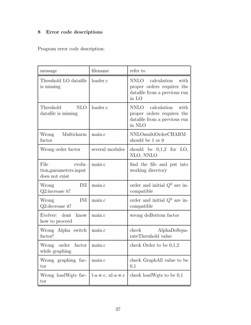
8 Error code descriptions

Program error code description:

message filename refer to

Threshold LO datafileis missing

loader.c NNLO calculation withproper orders requires thedatafile from a previous runin LO

Threshold NLOdatafile is missing

loader.c NNLO calculation withproper orders requires thedatafile from a previous runin NLO

Wrong Multicharmfactor

main.c NNLOmultiOrderCHARMshould be 1 or 0

Wrong order factor several modules should be 0,1,2 for LO,NLO, NNLO

File evolu-tion parameters.inputdoes not exist

main.c find the file and put intoworking directory

Wrong INIQ2:increase it!

main.c order and initial Q2 are in-compatible

Wrong INIQ2:decrease it!

main.c order and initial Q2 are in-compatible

Evolver: dont knowhow to proceed

main.c wrong doBottom factor

Wrong Alpha switchfactor!

main.c check AlphaDoSepa-rateThreshold value

Wrong order factorwhile graphing

main.c check Order to be 0,1,2

Wrong graphing fac-tor

main.c check GraphAll value to be0,1

Wrong loadWgts fac-tor

l-a-w.c, nl-a-w.c check loadWgts to be 0,1

37

9 Conclusions

We have presented a multifunctional code for the direct x-space method ofsolving the spin-averaged evolution equations for parton densities. The dis-tinctive features of this code include analytic computation of the LO, NLOand NNLO weights, NNLO heavy flavor threshold matching and NNLO evo-lution.

The code is very fast and accurate. For example for grid sizes not exceeding200 in Q2 and 150 in x the NLO calculation with full weighs computed forthree values of nf and up to five decimal accuracy has a runtime well below200 seconds. Also it is the only code that does the proper NNLO evolutionwith NNLO heavy flavor matching conditions.

The program is also easy to use and complete documentation is available. Thecode is well-tested both on specific test functions (e.g. see [16]) and on actualdensities (e.g. see [25]) in all (LO, NLO and NNLO) orders.

10 Acknowledgments

The work was partially supported by the National Science Foundation grantPHY-9722101. We thank Michael Botje for valuable comments on his methodof solving the evolution equations and providing us with his evolution code.We also thank Andreas Vogt for help with testing the code in NNLO and forproviding comparison data. Thanks are also due to Brian Harris for testingthe code and comments on the manuscript.

38

A Appendix A

Here we give the NNLO parametrizations of the splitting functions from [29].Note that L0 = ln z and L1 = ln(1 − z).

First the parametrizations for the non-singlet splitting functions P(2)±NS are:

P(2)−NS,A(z)= 1185.229 (1 − z)−1

+ + 1365.458 δ(1 − z) − 157.387 L21 − 2741.42 z2

− 490.43 (1 − z) + 67.00 L20 + 10.005 L3

0 + 1.432 L40

+ Nf {−184.765 (1 − z)−1+ − 184.289 δ(1 − z) + 17.989 L2

1 + 355.636 z2

− 73.407 (1 − z)L1 + 11.491 L20 + 1.928 L3

0} + P(2)NS,2(z),

P(2)−NS,B(z)= 1174.348 (1 − z)−1

+ + 1286.799 δ(1 − z) + 115.099 L21 + 1581.05 L1

+ 267.33 (1 − z) − 127.65 L20 − 25.22 L3

0 + 1.432 L40

+ Nf {−183.718 (1 − z)−1+ − 177.762 δ(1 − z) + 11.999 L2

1 + 397.546 z2

+ 41.949 (1 − z) − 1.477 L20 − 0.538 L3

0} + P(2)NS,2(z), (A.1)

and

P(2)+NS,A(z)= 1183.762 (1 − z)−1

+ + 1347.032 δ(1 − z) + 1047.590 L1 − 843.884 z2

− 98.65 (1 − z) − 33.71 L20 + 1.580 (L4

0 + 4L30)

+ Nf {−183.148 (1 − z)−1+ − 174.402 δ(1 − z) + 9.649 L2

1 + 406.171 z2

+ 32.218 (1 − z) + 5.976 L20 + 1.60 L3

0} + P(2)NS,2(z),

P(2)+NS,B(z)= 1182.774 (1 − z)−1

+ + 1351.088 δ(1 − z) − 147.692 L21 − 2602.738 z2

− 170.11 + 148.47 L0 + 1.580 (L40 − 4 L3

0)

+ Nf {−183.931 (1 − z)−1+ − 178.208 δ(1 − z) − 89.941 L1 + 218.482 z2

+ 9.623 + 0.910 L20 − 1.60 L3

0} + P(2)NS,2(z) . (A.2)

The parametrizations for P(2),SNS (z) and P

(2)PS (z) are

P(2)SNS,A(z)=Nf {(1 − z)(−1441.57 z2 + 12603.59 z − 15450.01) + 7876.93 zL2

0

− 4260.29 L0 − 229.27 L20 + 4.4075 L3

0}P

(2)SNS,B(z)=Nf {(1 − z)(−704.67 z3 + 3310.32 z2 + 2144.81 z − 244.68)

+ 4490.81 z2L0 + 42.875 L0 − 11.0165 L30}, (A.3)

and

P(2)PS,A(z)= Nf {(1 − z)(−229.497 L1 − 722.99 z2 + 2678.77− 560.20 z−1)

39

+ 2008.61 L0 + 998.15 L20 − 3584/27 z−1L0} + P

(2)PS,2(z),

P(2)PS,B(z)= Nf {(1 − z)(73.845 L2

1 + 305.988 L1 + 2063.19 z − 387.95 z−1)

+ 1999.35 zL0 − 732.68 L0 − 3584/27 z−1L0}+ P

(2)PS,2(z), (A.4)

with

P(2)PS,2(z)=N2

f {(1 − z)(−7.282 L1 − 38.779 z2 + 32.022 z − 6.252 + 1.767 z−1)

+ 7.453 L20} . (A.5)

Next we show the parametrizations of the off-diagonal singlet splitting func-tions:

P(2)qg,A(z)=Nf {−31.830 L3

1 + 1252.267 L1 + 1999.89 z + 1722.47 + 1223.43 L20

− 1334.61 z−1 − 896/3 z−1L0} + P(2)qg,2(z),

P(2)qg,B(z)=Nf {19.428 L4

1 + 159.833 L31 + 309.384 L2

1 + 2631.00 (1 − z)

− 67.25 L20 − 776.793 z−1 − 896/3 z−1L0} + P

(2)qg,2(z), (A.6)

with

P(2)qg,2(z)=N2

f {−0.9085 L21 − 35.803 L1 − 128.023 + 200.929 (1 − z)

+ 40.542 L0 + 3.284 z−1} , (A.7)

and

P(2)gq,A(z)= 13.1212 L4

1 + 126.665 L31 + 308.536 L2

1 + 361.21 − 2113.45 L0

− 17.965 z−1L0 + Nf {2.4427 L41 + 27.763 L3

1 + 80.548 L21

− 227.135 − 151.04 L20 + 65.91 z−1L0} + P

(2)gq,2(z),

P(2)gq,B(z)= −4.5108 L4

1 − 66.618 L31 − 231.535 L2

1 − 1224.22 (1 − z) + 240.08 L20

+ 379.60 z−1(L0 + 4) + Nf{−1.4028 L41 − 11.638 L3

1 + 164.963 L1

− 1066.78 (1 − z) − 182.08 L20 + 138.54 z−1(L0 + 2)}

+ P(2)gq,2(z), (A.8)

with

P(2)gq,2(z)=N2

f {1.9361 L21 + 11.178 L1 + 11.632 − 15.145 (1 − z) + 3.354 L0

− 2.133 z−1} . (A.9)

40

Last we show the parametrizations of the diagonal singlet splitting functions

P(2)gg,A(z)= 2626.38 (1 − z)−1

+ + 4424.168 δ(1 − z) − 732.715 L21 − 20640.069 z

− 15428.58 (1 − z2) − 15213.60 L20 + 16700.88 z−1 + 2675.85 z−1L0

+ Nf {−415.71 (1 − z)−1+ − 548.569 δ(1 − z) − 425.708 L1 + 914.548 z2

− 1122.86 − 444.21 L20 + 376.98 z−1 + 157.18 z−1L0}

+ P(2)gg,2(z),

P(2)gg,B(z)= 2678.22 (1 − z)−1

+ + 4590.570 δ(1 − z) + 3748.934 L1 + 60879.62 z

− 35974.45 (1 + z2) + 2002.96 L20 + 9762.09 z−1 + 2675.85 z−1L0

+ Nf {−412.00 (1 − z)−1+ − 534.951 δ(1 − z) + 62.630 L2

1 + 801.90

+ 1891.40 L0 + 813.78 L20 + 1.360 z−1 + 157.18 z−1L0}

+ P(2)gg,2(z), (A.10)

with

P(2)gg,2(z)=N2

f {−16/9 (1 − z)−1+ + 6.4882 δ(1 − z) + 37.6417 z2 − 72.926 z

+ 32.349 − 0.991 L20 + 2.818 z−1} . (A.11)

41

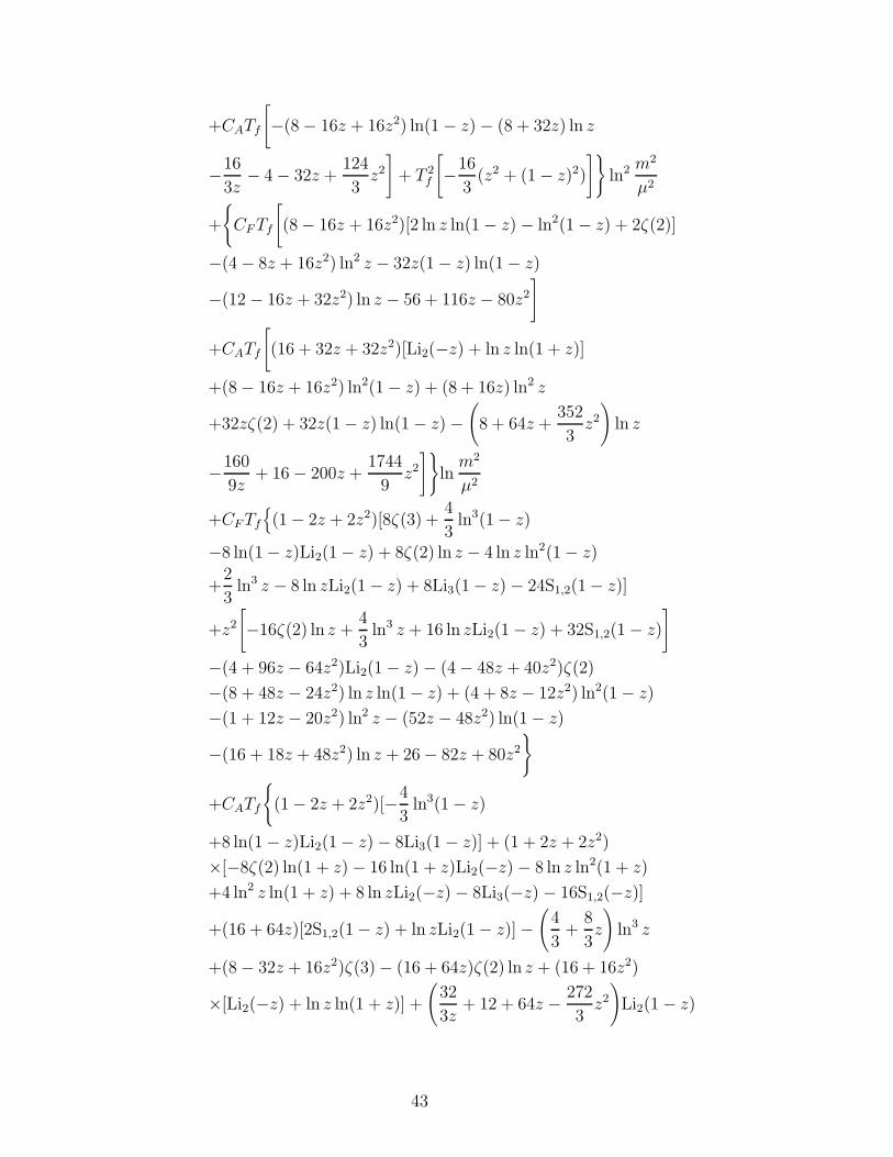
B Appendix B

Shown below are the renormalized OME’s used for threshold matching calcula-tions in NLO and NNLO (they correspond to the unrenormalized expressionsgiven in Appendix C of [36] and in Appendix A of [30]). All OME’S have beenrenormalized in the MS-scheme.

In particular the renormalized coupling αs is presented in the above schemefor nf +1 light flavors. Here the heavy quark H = (c, b) is treated on the samefooting as the light flavors and it is not decoupled from the running couplingin the VFNS approach. The (αs/4π)2 coefficient in the heavy-quark OME APS

Hq

is given by

APS,(2)Hq

(

m2

µ2

)

= CFTf

{[

−8(1 + z) ln z − 16

3z− 4

+4z +16

3z2

]

ln2 m2

µ2+

[

8(1 + z) ln2 z −(

8 + 40z +64

3z2

)

ln z

−160

9z+ 16 − 48z +

448

9z2

]

lnm2

µ2

+(1 + z)

[

32S1,2(1 − z) + 16 ln zLi2(1 − z) − 16ζ(2) ln z

−4

3ln3 z

]

+

(

32

3z+ 8 − 8z − 32

3z2

)

Li2(1 − z)

+

(

−32

3z− 8 + 8z +

32

3z2

)

ζ(2) +

(

2 + 10z +16

3z2

)

ln2 z

−(

56

3+

88

3z +

448

9z2

)

ln z − 448

27z− 4

3− 124

3z +

1600

27z2

}

, (B.1)

The αs/4π and the (αs/4π)2 coefficients of the heavy quark OME’s ASHg are

AS,(1)Hg

(

m2

µ2

)

= Tf

[

−4(z2 + (1 − z)2) lnm2

µ2

]

, (B.2)

and

AS,(2)Hg

(

m2

µ2

)

=

{

CFTf [(8 − 16z + 16z2) ln(1 − z)

−(4 − 8z + 16z2) ln z − (2 − 8z)]

42

+CATf

[

−(8 − 16z + 16z2) ln(1 − z) − (8 + 32z) ln z

−16

3z− 4 − 32z +

124

3z2

]

+ T 2f

[

−16

3(z2 + (1 − z)2)

]}

ln2 m2

µ2

+

{

CF Tf

[

(8 − 16z + 16z2)[2 ln z ln(1 − z) − ln2(1 − z) + 2ζ(2)]

−(4 − 8z + 16z2) ln2 z − 32z(1 − z) ln(1 − z)

−(12 − 16z + 32z2) ln z − 56 + 116z − 80z2

]

+CATf

[

(16 + 32z + 32z2)[Li2(−z) + ln z ln(1 + z)]

+(8 − 16z + 16z2) ln2(1 − z) + (8 + 16z) ln2 z

+32zζ(2) + 32z(1 − z) ln(1 − z) −(

8 + 64z +352

3z2

)

ln z

−160

9z+ 16 − 200z +

1744

9z2

]}

lnm2

µ2

+CF Tf

{

(1 − 2z + 2z2)[8ζ(3) +4

3ln3(1 − z)

−8 ln(1 − z)Li2(1 − z) + 8ζ(2) ln z − 4 ln z ln2(1 − z)

+2

3ln3 z − 8 ln zLi2(1 − z) + 8Li3(1 − z) − 24S1,2(1 − z)]

+z2

[

−16ζ(2) ln z +4

3ln3 z + 16 ln zLi2(1 − z) + 32S1,2(1 − z)

]

−(4 + 96z − 64z2)Li2(1 − z) − (4 − 48z + 40z2)ζ(2)

−(8 + 48z − 24z2) ln z ln(1 − z) + (4 + 8z − 12z2) ln2(1 − z)

−(1 + 12z − 20z2) ln2 z − (52z − 48z2) ln(1 − z)

−(16 + 18z + 48z2) ln z + 26 − 82z + 80z2

}

+CATf

{

(1 − 2z + 2z2)[−4

3ln3(1 − z)

+8 ln(1 − z)Li2(1 − z) − 8Li3(1 − z)] + (1 + 2z + 2z2)

×[−8ζ(2) ln(1 + z) − 16 ln(1 + z)Li2(−z) − 8 ln z ln2(1 + z)

+4 ln2 z ln(1 + z) + 8 ln zLi2(−z) − 8Li3(−z) − 16S1,2(−z)]

+(16 + 64z)[2S1,2(1 − z) + ln zLi2(1 − z)] −(

4

3+

8

3z

)

ln3 z

+(8 − 32z + 16z2)ζ(3) − (16 + 64z)ζ(2) ln z + (16 + 16z2)

×[Li2(−z) + ln z ln(1 + z)] +

(

32

3z+ 12 + 64z − 272

3z2

)

Li2(1 − z)

43

−(

12 + 48z − 260

3z2 +

32

3z

)

ζ(2) − 4z2 ln z ln(1 − z)

−(2 + 8z − 10z2) ln2(1 − z) +

(

2 + 8z +46

3z2

)

ln2 z

+(4 + 16z − 16z2) ln(1 − z) −(

56

3+

172

3z +

1600

9z2

)

ln z

−448

27z− 4

3− 628

3z +

6352

27z2

}

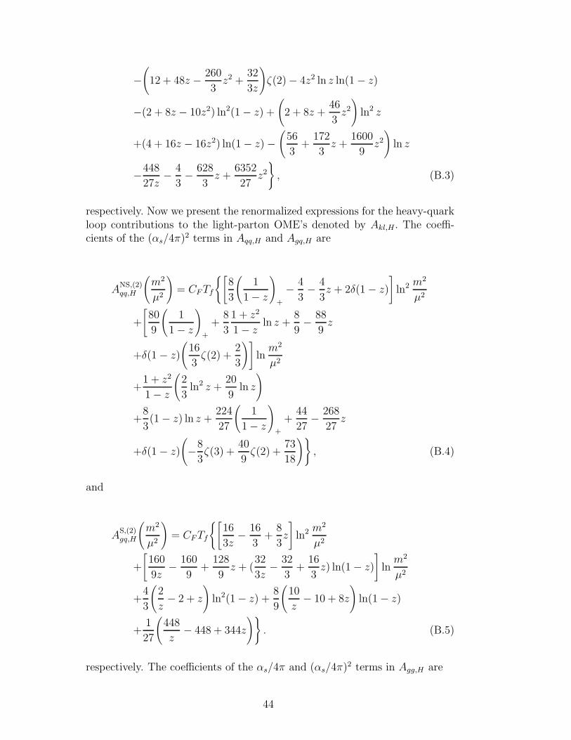
, (B.3)

respectively. Now we present the renormalized expressions for the heavy-quarkloop contributions to the light-parton OME’s denoted by Akl,H. The coeffi-cients of the (αs/4π)2 terms in Aqq,H and Agq,H are

ANS,(2)qq,H

(

m2

µ2

)

= CFTf

{[

8

3

(

1

1 − z

)

+

− 4

3− 4

3z + 2δ(1 − z)

]

ln2 m2

µ2

+

[

80

9

(

1

1 − z

)

+

+8

3

1 + z2

1 − zln z +

8

9− 88

9z

+δ(1 − z)

(

16

3ζ(2) +

2

3

)]

lnm2

µ2

+1 + z2

1 − z

(

2

3ln2 z +

20

9ln z

)

+8

3(1 − z) ln z +

224

27

(

1

1 − z

)

+

+44

27− 268

27z

+δ(1 − z)

(

−8

3ζ(3) +

40

9ζ(2) +

73

18

)}

, (B.4)

and

AS,(2)gq,H

(

m2

µ2

)

= CFTf

{[

16

3z− 16

3+

8

3z

]

ln2 m2

µ2

+

[

160

9z− 160

9+

128

9z + (

32

3z− 32

3+

16

3z) ln(1 − z)

]

lnm2

µ2

+4

3

(

2

z− 2 + z

)

ln2(1 − z) +8

9

(

10

z− 10 + 8z

)

ln(1 − z)

+1

27

(

448

z− 448 + 344z

)}

. (B.5)

respectively. The coefficients of the αs/4π and (αs/4π)2 terms in Agg,H are

44

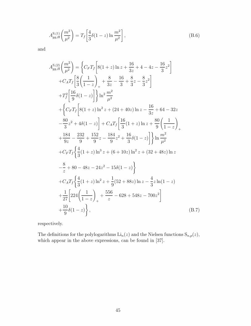
AS,(1)gg,H

(

m2

µ2

)

= Tf

[

4

3δ(1 − z) ln

m2

µ2

]

, (B.6)

and

AS,(2)gg,H

(

m2

µ2

)

=

{

CF Tf

[

8(1 + z) ln z +16

3z+ 4 − 4z − 16

3z2

]

+CATf

[

8

3

(

1

1 − z

)

+

+8

3z− 16

3+

8

3z − 8

3z2

]

+T 2f

[

16

9δ(1 − z)

]}

ln2 m2

µ2

+

{

CF Tf

[

8(1 + z) ln2 z + (24 + 40z) ln z − 16

3z+ 64 − 32z

−80

3z2 + 4δ(1 − z)

]

+ CATf

[

16

3(1 + z) ln z +

80

9

(

1

1 − z

)

+

+184

9z− 232

9+

152

9z − 184

9z2 +

16

3δ(1 − z)

]}

lnm2

µ2

+CF Tf

{

4

3(1 + z) ln3 z + (6 + 10z) ln2 z + (32 + 48z) ln z

−8

z+ 80 − 48z − 24z2 − 15δ(1 − z)

}

+CATf

{

4

3(1 + z) ln2 z +

1

9(52 + 88z) ln z − 4

3z ln(1 − z)

+1

27

[

224

(

1

1 − z

)

+

+556

z− 628 + 548z − 700z2

]

+10

9δ(1 − z)

}

, (B.7)

respectively.

The definitions for the polylogarithms Lin(z) and the Nielsen functions Sn,p(z),which appear in the above expressions, can be found in [37].

45

References

[1] G. Altarelli and G. Parisi, Nucl. Phys. B126, 298 (1977); V.N. Gribov andL.N.Lipatov, Sov. J. Nucl. Phys. 15 438, 675, (1972); Yu. Dokshitser, Sov.Phys. JETP 46, 641 (1977).

[2] R.G. Roberts, in The Structure of the Proton, Cambridge University Press(1993).

[3] R.K. Ellis, W.J. Stirling and B.R. Webber, in QCD and Collider Physics,

Cambridge University Press (1996), Chapter 4.3.

[4] H. Georgi and H.D. Politzer, Phys. Rev. D9, 416 (1974).

[5] D.J. Gross and F. Wilczek, Phys. Rev D9, 980 (1974).

[6] E. G. Floratos, D.A. Ross and C.T. Sachrajda, Nucl. Phys. B129, 66 (1977)Erratum B139, 545 (1978); ibid B152, 493 (1979).

[7] A. Gonzales-Arroyo, C. Lopez and F.J. Yndurain, Nucl. Phys. B153, 161(1979); A. Gonzales-Arroyo and C. Lopez, Nucl. Phys. B166, 429 (1980).

[8] E.G. Floratos, C. Kounnas and R. Lacaze, Phys. Lett. B98, 89, 285, (1981);ibid. Nucl. Phys. B192, 417 (1981).

[9] R. Hamberg and W.L. van Neerven, Nucl. Phys. B359, 343 (1991).

[10] S.A. Larin, T. van Ritbergen and J.A.M. Vermaseren, Nucl. Phys. B427, 41(1994), [hep-ph/9411260]; S.A. Larin et al., Nucl. Phys. B492, 338 (1997), [hep-ph/9605317].

[11] J.F. Bennett and J.A Gracey, Nucl. Phys. B417, 241 (1998); J.A. Gracey, Phys.Lett. B322, 141 (1994), [hep-ph/9401214].

[12] W.L. van Neerven and A. Vogt, [hep-ph/9907472].

[13] M. Miyama and S. Kumano, Comput. Phys. Commun. 94, 185 (1996), [hep-ph/9508246]; M. Hirai, S. Kumano and M. Miyama, Comput. Phys. Commun.108, 38 (1998), [hep-ph/9707220].

[14] M. Botje, QCDNUM16: A fast QCD evolution program, ZEUS N5te 97-066.

[15] C. Pascaud and F. Zomer, H1 Note H1-11/94-404; V. Barone, C. Pascaud andF. Zomer, [hep-ph/9907512].

[16] J. Blumlein, S. Riemersma, W.L. van Neerven and A. Vogt, Nucl. Phys. B(Proc.Suppl.) 51C, 96 (1996), [hep-ph/9609217];J. Blumlein, M. Botje, C. Pascaud, S. Riemersma, W.L. van Neerven, A. Vogtand F. Zomer, in Proceedings of the Workshop on Future Physics at HERA

edited by G. Ingelman, A. De Roeck and R. Klanner, Hamburg, Germany, 25-26 Sep. 1995, p. 23, DESY 96-199, [hep-ph/9609400].

46

[17] A.D. Martin, R.G. Roberts, W.J. Stirling and R. Thorne, Eur. Phys. J. C4,463 (1998), [hep-ph/9803445].

[18] H.L. Lai, J. Huston, S. Kuhlmann, J. Morfın, F. Olness, J. Owens, J. Pumplinand W.K. Tung, [hep-ph/9903282].

[19] G. Curci, W. Furmanski and R. Petronzio, Nucl. Phys. B175, 27 (1980); W.Furmanski and R. Petronzio, Phys. Lett. B97 437, (1980); ibid. Z. Phys. C11,293 (1982); the relevant NLO formulae are presented in a convenient form inref. 2.

[20] C. Coriano and S. Savkli, Comput. Phys. Commun. 118, 236 (1999), [hep-ph/9803336].

[21] S. Riemersma, unpublished.

[22] M. Gluck, E. Reya and A. Vogt, Eur. Phys. J. C5, 461 (1998), [hep-ph/9806404].

[23] H. Plothow-Besch, PDFLIB version 8.04, available from CERNLIB athttp://wwwinfo.cern.ch/asdoc.

[24] M.A.G. Aivazis, J.C. Collins, F.I. Olness and W.-K. Tung, Phys. Rev. D50,3102 (1994), [hep-ph/9312319].

[25] A. Chuvakin, J. Smith and W. van Neerven, Phys. Rev. D61, 096004 (2000),[hep-ph/9910250].

[26] A. Chuvakin, J. Smith and W. van Neerven, Phys.Rev. D62, 036004 (2000),[hep-ph/0002011].

[27] A. Chuvakin, J. Smith and B.W. Harris, Eur.Phys.J. C18,547 (2001), [hep-ph/0010350].

[28] W.L. van Neerven; A. Vogt, [hep-ph/9907472].

[29] W.L. van Neerven; A. Vogt, [hep-ph/0007362].

[30] M. Buza, Y. Matiounine, J. Smith and W.L. van Neerven, Eur. Phys. J. C1,301 (1998); Phys. Lett. B411,211 (1997), [hep-ph/9612398].

[31] W. Bernreuther and W. Wetzel, Nucl. Phys. B197, 228 (1982); Erratum-ibid513, 758 (1998); W. Bernreuther, Annals of Physics, 151, 127 (1983).

[32] S.A. Larin, T. van Ritbergen and J.A.M. Vermaseren, Nucl. Phys. B438,278 (1995), [hep-ph/9411260]; see also K.G. Chetyrkin, B.A. Kniehl and M.Steinhauser, Phys. Rev. Lett. 79, 2184 (1997), [hep-ph/9706430].

[33] A. Chuvakin, J. Smith, Phys. Rev. D61, 114018 (2000); [hep-ph/9911504].

[34] R. Piessens, Angew. Informatik 9, 399 (1973).

[35] K.S. Kolbig, J.A. Mignaco and E. Remiddi, BIT 10, 38 (1971);K.S. Kolbig, SIAM J. Math. Anal. 17 1232 (1986);see http://wwwinfo.cern.ch/asdoc/shortwrupsdir/c31/top.html.

47

[36] M. Buza, Y. Matiounine, J. Smith, R. Migneron, and W.L. van Neerven, Nicl.Phys. B472, 611 (1996), [hep-ph/9601302].

[37] L. Lewin, ”Polylogarithms and Associated Functions”, North Holland,Amsterdam, 1983;R. Barbieri, J.A. Mignaco and E. Remiddi, Nuovo Cimento 11A (1972) 824;A. Devoto and D.W. Duke, Riv. Nuovo. Cimento Vol. 7,N. 6 (1984) 1.

48

Figure Captions

Fig. 1. The gluon density xgNNLO(4, x, µ2) in the range 10−5 < x < 1 forµ2 = 2, 3, 4, 5, 10 and 20 in units of (GeV2)2,

Fig. 2. The singlet density xΣNNLO(4, x, µ2) in the range 10−5 < x < 1 forµ2 = 2, 3, 4, 5, 10 and 20 in units of (GeV2)2,

Fig. 3. The nonsinglet quark density xσNNLO(4, x, µ2)a, where σ = (u+ u)/2,in the range 10−5 < x < 1 for µ2 = 2, 3, 4, 5, 10 and 20 in units of (GeV2)2,

Fig. 4. The charm quark density xcNNLO(4, x, µ2) the range 10−5 < x < 1 forµ2 = 1.96, 2, 3, 4, 5, 10 and 20 in units of (GeV2)2,

49