EXELFS revisited

Perg .mon PII: S0968-4328(96)00044-3

EXELFS Revisited

Micron Vol. 27. No. 6, pp. 449 466, 1996 1997 Elsevier Science Ltd

All rights reserved. Printed in Great Britain I)968 4328/96 $32.00+0.00

M. SARIKAYA,* M. QIAN* and E. A. S T E R N t

*Departments o f Materials" Science and Engineering, Box." 352120, University o f Washington, Seattle, WA 98195, U.S.A. +Department (~[ Physics, Box." 351560, University o[ Washington. Seattle, W A 98195. U.S.A.

Abstract EXELFS (Extended Electron Energy Loss Fine Structure) spectroscopy contains the same local atomic structural information as XAFS (i.e. short-range order), but also it has good low-Z elemental sensitivity, much higher spatial resolution (nanoscale) and the capacity of combining other high spatial resolution TEM measurements together with EXELFS. Until recently, due to poor quality of the EELS data, however, the EXELFS technique has not been developed to its full advantage. Various new methods to improve the data acquisition technique have been introduced, which include on-line removal of channel-to-channel gain variation and correction of dark-current background under real acquisition conditions: also aligning and accumulat ing a virtually unlimited number of spectra while monitor ing the thickness change (due to sample drift), radiation damage and change in energy resolution during measurements . A systematic data analysis procedure has been developed which includes removing edge overlapping, z-data normalization and adopting the U W X A F S data analysis software package to perform EXELFS data analysis at the same level of sophistication. Pure a luminium and silicon carbide were used as calibration materials. A complex carbonitride material with unknown (but theoretically predicted) structure and thin-film nickel oxide samples were used for further demonstrat ion of the technique's current capabilities as a tool for structural characterization in a wide range of materials applications. The K-edges of A1 (at 1560 eV), Si (1839 eV), O (532 eV), N (402 eV), C (284 eV) were used for EXELFS analysis; for Ni, the L , 3 edge (at 855 eV) was used. EXELFS spectra were measured and analyzed using theoretical calculations and r-space non-linear least-square fits to determine the structural parameters. Good agreements with the known and predicted structures were obtained. !" 1997 Elsevier Science Ltd

Key words: EXELFS, EELS. XAFS, A1, SiC, nickel oxide, carbonitride, atomic structure, nanostructure.

CONTENTS I. Introduction ........................................................................................................................................................................................................... 449

A. Background .................................................................................................................................................................................................... 449 B. Problems traditionally associated with EXELFS technique ..................................................................................................................... 450

II. New developments in eel spectrum aquisition .................................................................................................................................................. 450 A. CCGV correction under real acquisition conditions .................................................................................................................................. 450 B. On-line acquisition of a large number of spectra ....................................................................................................................................... 452 C. Some important aspects of long-duration date acquisition ....................................................................................................................... 452

IlI. Further developments in EXELFS data analysis ............................................................................................................................................. 454 A. Improvement ot" spectral resolution ............................................................................................................................................................. 455 B. Extraction of single core-loss scattering spectrum ..................................................................................................................................... 455 C. Background removal ...................................................................................................................................................................................... 455 D Normalization ................................................................................................................................................................................................. 455 E Separation of overlapping edges ................................................................................................................................................................... 456

IV. Applications ........................................................................................................................................................................................................... 456 A. Aluminium ....................................................................................................................................................................................................... 456 B. Bulk silicon carbide ........................................................................................................................................................................................ 457 C. Polycrystalline thin-film nickel oxide ........................................................................................................................................................... 459 D. Nanocrystalline carbonitride ......................................................................................................................................................................... 461

V. Summary and concluding remarks ..................................................................................................................................................................... 463 VI. Future prospects ................................................................................................................................................................................................... 464

Acknowledgements ............................................................................................................................................................................................... 464 References .............................................................................................................................................................................................................. 464

I. INTRODUCTION

A. Background

It is well known that X-ray Absorption Fine Structure (XAFS) is a unique technique for short-range order and atomic structure determination (Stern and Heald, 1983; Sayers et al., 1971). XAFS is an element-specific technique providing partial pair distribution function (PPDF). XAFS measures the local structure, so it can be applied equally well to amorphous, locally-ordered and fully crystalline materials. It studies the fine oscillation structure of the absorption coefficient past an absorption edge when the X-ray photon energy is just sufficient to free core

449

electrons from an atom. As the X-ray photon energy is increased, excess energy is imparted to the photoelectron, consequently varying the wavelength of its wave function. The final state wave function of the photoelectron is the interference of the outgoing portion of the wave function with the portion backscattered from the', surrounding atoms. The phase difference between these two functions varies as the photoelectron wavelength changes, introducing fine structure in the absorption. The single scattering formula (assuming Gaussian disorder) is

m N. , n, ~,- z(k)=S0 T ~ 7 . ~. ~ t ,(2k) e e stn[2kR,+6i(k) ],

47rh-k i R~ . . . . (l)

450 M. Sarikaya et al.

and

z (k) =l~(k) - It°(k), (2) /x0(k)

where/~(k) is the measured absorption coefficient, including fine structure,/lo(k ) is the smooth background of the absorption coefficient, x(k) is the XAFS function, Ny is the co-ordination number of the j'th shell, R] is the distance of j-shell atoms, a 2 is the mean squared disorder about R], 2 is the mean free path of the photoelectron, and 6 is the phase shift introduced by the central and backscattered atoms.

Some of the major features of XAFS are the following: the local atomic arrangement is determined about each type of atom separately by tuning the X-rays to its characteristic absorption energy edge; the numbers and types of surrounding atoms up to the 4th nearest neighbors and beyond can be determined; the average distance of atoms can be ascertained with an accuracy of t0.01 ~ and the distribution about the average (a, Debye-Waller factor) can be determined with a resolution of 0.1 ~; angular dependence of the distribution of atoms can be obtained in some special cases; when three or more atoms are nearly collinear, three-body corre- lations can be measured, including the angle from col- linearity. The analysis is relatively straightforward and simple so that only small computers are required and the analysis can be accomplished in a short time. Measuring near-edge fine structure adds electronic binding information such as the valence of the absorbing atom. The XAFS technique is limited to determining short-range- order and loses its capabilities if a, the rms distribution of atoms about their average position, is greater than about 0.15 ~. Fortunately, the short-range atomic spacing is rarely that disordered, at least for the first neighbors.

XAFS has been an important tool in determining the local atomic structures of materials in the condensed matter. Recently, the capability to analyze accurately the structure out to fourth nearest neighbors and further was made possible by the introduction of both accurate theoretical calculations (Mustre de Leon et al., 1991; Rehr et al., 1991, 1992) of the multiple scattering suffered by the excited photoelectrons and software to relate these calculations to the data (Stern et al., 1995a).

It was appreciated some time ago that the same XAFS information is also present in the extended electron energy loss fine structure (EXELFS) from high energy electrons passing through matter (Leapman and Cosslett, 1976; Johnson et al., 1981). When applicable, EXELFS has several advantages over XAFS. For example, it has greater spatial resolution (determined by the electron probe size) and can be used to investigate phases that are spatially inhomogeneous, such as in complex nanostructured materials. In addition, the region being investigated can be characterized fully by other capabilities of the TEM such as imaging (including atomic-resolution electron microscopy: AREM), diffraction (including convergent beam electron diffraction:

CBED) and quantitative elemental compositional analysis (most commonly by using both energy dispersive X-ray spectroscopy and electron energy loss spectroscopy, EDS and EELS, respectively) (Sarikaya, 1992). The EXELFS technique is optimum for measuring losses in the 0-1500 eV range. This is just the soft X-ray range which is most difficult to investigate by XAFS using synchrotron radiation sources.

B. Problems traditionally associated with E X E L F S technique

In spite of the promise and availability of a commer- cial parallel electron energy loss (PEEL) detector which increases the data collection rate by two orders of magnitude over the older serial detectors (Krivanek et al., 1987), the EXELFS technique has not yet been as fully exploited for structure determination as XAFS. The reasons are:

(1) the lack of high quality EEL spectra to accurately measure the weak fine structure. To correct this situation requires obtaining high statistics while correcting the systematic errors introduced by the instrument, including energy and specimen drift, dark current and channel-to-channel gain variation (CCGV) of the parallel energy loss detector;

(2) the need to monitor radiation damage and keep it below values that can produce significant changes in structure.

(3) the need to utilize a proven data analysis package to evaluate the EXELFS data, which includes normalizing the data by the correct background, separating the overlapping edges, and correctly applying the well-developed XAFS data analysis technique to EXELFS.

In the following sections, developments in the acquisition and analysis of the EXELFS data which overcome these difficulties are described and summarized.

II. NEW DEVELOPMENTS IN EEL SPECTRUM ACQUISITION

A systematic method to address the problems listed above has been developed (Qian et al., 1993a, 1995a) using software entitled UWEXELFS 1.0 (Sarikaya et al., 1995). With this new method, it is possible to continu- ously acquire EELS data over several hours to accumulate high enough counts (106 counts per channel or more) with minimum distortion in the spectra due to CCGV and all other instabilities.

A. C C G V correction under real acquisition conditions

The photodiode array in the PEELS system contains 1024 channels, each with an active area of

EXELFS Revisited 451

D e t e c t o r ce i l s Dispersed electron beam

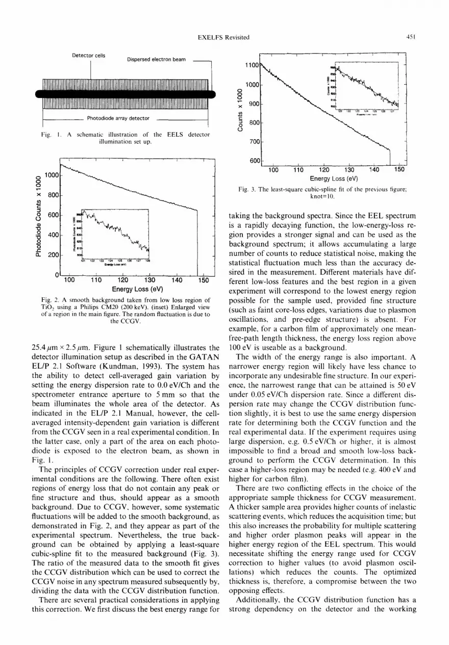
Fig. 1. A schematic illustration of the EELS detector illumination set up.

o 1000 0 0

× 800 m

o 600 o

• ~ 400 0

200

L I ~ L J

L ~ leVI

li00 T ~ 11o 12o ' 150 Energy Loss (eV)

Fig. 2. A smooth background taken from low loss region of TiO 2 using a Philips CM20 (200 keV). (inset) Enlarged view of a region in the main figure. The random fluctuation is due to

the CCGV.

25.4pm x 2.5 pro. Figure 1 schematically illustrates the detector illumination setup as described in the GATA N EL/P 2.1 Software (Kundman, 1993). The system has the ability to detect cell-averaged gain variation by setting the energy dispersion rate to 0.0 eV/Ch and the spectrometer entrance aperture to 5 mm so that the beam illuminates the whole area of the detector. As indicated in the EL/P 2.1 Manual, however, the cell- averaged intensity-dependent gain variation is different from the CCGV seen in a real experimental condition. In the latter case, only a part of the area on each photodiode is exposed to the electron beam, as shown in Fig. 1.

The principles of CCGV correction under real experimental conditions are the following. There often exist regions of energy loss that do not contain any peak or fine structure and thus, should appear as a smooth background. Due to CCGV, however, some systematic fluctuations will be added to the smooth background, as demonstrated in Fig. 2, and they appear as part of the experimental spectrum. Nevertheless, the true background can be obtained by applying a least-square cubic-spline fit to the measured background (Fig. 3). The ratio of the measured data to the smooth fit gives the CCGV distribution which can be used to correct the CCGV noise in any spectrum measured subsequently by, dividing the data with the CCGV distribution function.

There are several practical considerations in applying this correction. We first discuss the best energy range for

0 0 0

x

¢-

0 o

i i i i ~ i

1100 , ~ I ! 1000 i 9OO

80C '

7OO

60O 100 110 120 130 140 150

Energy Loss(eV) Fig. 3. The least-square cubic-spline fit o f t h e previous figure;

knot=10.

taking the background spectra. Since the EEL spectrum is a rapidly decaying function, the low-energy-loss region provides a stronger signal and can be used as the background spectrum; it allows accumulating a large number of counts to reduce statistical noise, making the statistical fluctuation much less than the accuracy de- sired in the measurement. Different materials have different low-loss features and the best region in a given experiment will correspond to the lowest energy region possible for the sample used, provided fine structure (such as faint core-loss edges, variations due to plasmon oscillations, and pre-edge structure) is absent. For example, for a carbon film of approximately one mean- free-path length thickness, the energy loss region above 100 eV is useable as a background.

The width of the energy range is also important. A narrower energy region will likely have less chance to incorporate any undesirable fine structure. In our experience, the narrowest range that can be attained is 50 eV under 0.05 eV/Ch dispersion rate. Since a different dispersion rate may change the CCGV distribution function slightly, it is best to use the same energy dispersion rate for determining both the CCGV function and the real experimental data. If the experiment requires using large dispersion, e.g. 0.5 eV/Ch or higher, it is almost impossible to find a broad and smooth low-loss background to perform the CCGV determination. In this case a higher-loss region may be needed (e.g. 400 eV and higher for carbon film).

There are two conflicting effects in the choice of the appropriate sample thickness for CCGV measurement. A thicker sample area provides higher counts of inelastic scattering events, which reduces the acquisition time; but this also increases the probability for mulliple scattering and higher order plasmon peaks will appear in the higher energy region of the EEL spectrum. This would necessitate shifting the energy range used for CCGV correction to higher values (to avoid plasmon oscillations) which reduces the counts. The optimized thickness is, therefore, a compromise between the two opposing effects.

Additionally, the CCGV distribution function has a strong dependency on the detector and the working


conditions. Fortunately, it has no specimen-dependence so it is possible to use just one appropriate material, such as carbon film, to perform the CCGV measurement, and then use this calibration for all other materials. There is a slight time dependence in applying this principle, but, in our experience, the instrumental stability remains sufficiently good for several weeks.

The last point to consider is the fact that a cubic-spline fit is not sensitive to any long range (low frequency) variations of the background, such as the readout profile and low-frequency variation of the detector gain distribution function. Fortunately, these variations can be corrected by the EL/P 'detector gain' calibration. There- fore, it is important that, before doing the CCGV measurement, all the calibrations necessitated by the EL/P software are done (such as detector background and detector gain calibrations). It is also critical to make sure that there is no detector charging effect remaining from the previous measurements.

B. On-line acquisition of a large number of spectra

As mentioned previously, the major problem in detecting a weak signal is that the statistical fluctuation may be close to or exceed the signal level that is being determined. The relative fluctuation of N independent measured events (counts) is:

AN 1 N - ~ " (3)

Assuming that the fine structure signal, S, is 1% of the total counts (as it is very often the case in EXELFS), then

S --,.~0.01. (4) N

For a well-distinguished signal in the spectrum, it is necessary that

S/N<ANIN (5) or

S AN - - ~ 1 0 - - (6) N N"

This means that N has to be of the order of 10 6. The maximum counts in an individually acquired

spectrum are 16 K counts/Ch because of detector satur- ation. In most cases, however, a single read-out contains much fewer counts/Ch due to: (1) low beam current, due to small probe or small spectrometer entrance aperture; (2) low inelastic scattering cross-section in higher energy-loss regions; (3) low concentration of the element of interest in impurity-determination type studies. The room for increasing the counts/Ch by increasing the single readout time is limited because of energy drift. To accumulate high enough counts, therefore, a sum over a large number of spectra is required. This involves a large

hard-disk space for off-line summation, causing the acquisition to be very slow. Consequently, the sample will be unnecessarily exposed to the electron beam, which increases the probability of radiation damage.

A major problem in on-line spectrum summation is spectral drift. There are many factors, such as instability of power supplies, environmental electrical and/or magnetic-field variations, instabilities in the electron source (e.g. filament temperature variation) and mechanical vibrations, that affect the stability of the measurement and the spectral drift. It is common for the spectrum to drift a few channels even during a ten-minute acquisition period. It should, therefore, be obvious that without a spectral alignment, a sum over a large number of spectra (which may require an hour or more) will smear out the signal. Our spectra-alignment strategy is based on the assumption that all spectra, acquired sequentially from the same specimen under the same experimental conditions, are correlated except for an energy drift. Once a particular feature is aligned, all the features of the spectra are aligned simultaneously.

The method of performing spectrum alignment is the following. Firstly, one chooses a prominent feature, e.g. a sharp ionization edge. Secondly, if the data have considerable noise, a low-pass filter would be used to smooth the data. Thirdly, one determines the peak position and the correct profile of the peak. Finally, the peak position and the profile of the peak for every newly-acquired spectrum are compared to identify the corresponding feature. This is followed by the determination of the energy shift; then the new spectrum is aligned back using this value with respect to the feature, and added to the previously summed spectrum. The accuracy of alignment depends on the sharpness of the edge and the statistical noise level. For a pronounced feature and 10 2 or more counts/Ch, the peak position can be determined well within the energy resolution, which is about 1.0-2.5 eV in our experiments.

C. Some important aspects of long-duration data acquisition

1. Monitoring the change in thickness

As demonstrated in Fig. 4, both the background and the fine structure of a spectrum may change with time, due to sample and beam drift during the long acquisition (often tens of minutes to a few hours duration). This introduces EELS data from regions of different thickness from the initially established one, and therefore causes unknown plural scattering contributions. Obviously, this will make the removal of plural scattering contribution impractical since it would require measuring a low-loss spectrum and doing a correction after every few readouts. It is important, therefore, to monitor any variation of sample thickness during a long-period acquisition.

The principle of monitoring the sample thickness during acquisition is the following: for simplicity, it is


8O

g to! × 60 q)

g 50 ID

O 40 ID " o ID =5 80 o

20 13-

10

0 ' 300 ' 350 ' 400 450 5()0 ' 550

Energy Loss (eV)

Fig. 4. Several C K-edge spectra taken from same region of a SiC sample. Both the background and fine structure changed due to sample and beam drift during a long acquisition (about

an hour).

2.5

o

2.0

15

e~

I.O g

0~ 0.5

E

0

~s(E+Ep) _J

i I i i i i

1500 1550 1600 1650 1700 1750 18.00 E (eV)

Fig. 5. Schematic illumination of the edge distortion due to double scattering. A measured spectrum ~d(E) can be viewed as a superimposition of two single-scattered spectra: q)s(E) and qb (E+E~,), ~s(E) has the true edge energy E,, and reduced amplitude (1 - x ) , where x is the percentage of double scattering, whereas ~+(E+Ep) has a shifted edge-energy (E.+Ep) and

an amplitude x, where Ep is the plasmon energy.

g O

x

¢/1

g o

0 =5

0

#_

12 ~

10

8

6

4

2

I I I L " I I

0-15 -10 -5 0 5 10 15 20

Energy Loss (eV)

Fig. 6. Two zero-loss spectra acquired before and after a long acquisition. A significant change in energy resolution can be

seen.

g O

x

E O o "O

O =5 o O ¢-.

n

250 -

+ 0 _

100

50 - ~

260 ' 280 ' 3dO 3:~0 ' 340 ' 360 ' 380 ' 400

Energy Loss (eV)

Fig. 7. Two carbon K-edge spectra from the same area of a SiC sample, corresponding to the different energy resolutions shown in Fig. 6. The effect of energy resolution is seen as a change to the core edge region, smearing out of sharp features.

variation occurred, one can pause the acquisition and readjust the sample to its original position.

assumed that the sample is thin enough so that only double scattering needs to be considered and that the plasmon peak can be approximately represented by a 6-function. The measured edge, distorted due to plural scattering, can be treated as a superimposition of two single-scattered spectra. One of these superimposed spectra has the true edge-energy E o and reduced amplitude (1 - . \ ) , where x denotes the percentage of double scattering. The other spectrum has a shifted edge-energy of (E,,+E v) and an amplitude x, where Ep~ 15 eV denotes the plasmon energy as shown in Fig. 5. From the figure, it is clear that there is an additional peak on the distorted spectrum located around (Eo+Ep) (here, E, denotes the white line position; i.e. the maximum near the edge) which is due to the plasmon scattering. Any change in sample-thickness will be indicated by measuring the relative change of the spectral heights at (Eo+Ev).

This measurement option has been incorporated into our AcqLong function (in the acquisition program) to monitor thickness variation so that if a large thickness

2. Monitoring variations of energy resolution

We have found that the energy resolution of the EELS spectrometer may change during spectrum acquisition. As an example, Fig. 6 shows two zero-loss spectra acquired before and after a long acquisition, demon- strating a significant change in energy resolution. There may be several reasons for the change; environmental electric and/or magnetic field variations and spectrometer instability are the most likely possibilities. The effect of worsened energy resolution on the core loss spectra is in a smearing-out of the sharp features, as displayed in Fig. 7. To monitor the variation of energy resolution, the AcqLong program is instructed to calculate the full width at half maximum of the white-line, and posts a warning message if there is a significant change. When this happens, one can temporarily stop the acquisition and compare the changes both at the white line and at (E,,+Ep). If the former has a significant change but the latter has not, the energy resolution has changed and

454 M. Sarikaya et aL

I ' I ' I ' I ~ I ' I

6000 -

5000 -

4000-

"~ 3000-

o 2000

tO00 ~

0 1800 1900 2000 21 O0 2200 2300

Energy loss (eV)

Fig. 8. (a) A silicon K-edge EEL spectrum of SiC acquired with a total of 50 readouts, each readout lasting 5 s. (b) A dark-current spectrum, acquired immediately after the Si K-edge spectrum, with same acquisition condition as specified in (a). (c) Removal of

darkcurrent background--subtract (b) from (a).

one can take proper actions, including realignment before resuming spectral measurement.

3. A flexible way to correct dark current

It is well known that the dark current of a detector is temperature dependent. The change is quite rapid at the beginning of an experiment, and takes one to two hours to stabilize. Therefore, it requires calibrating from time to time during an experiment.

Another issue related to dark current calibration is the non-linear relationship between the dark current counts and the acquisition time. For simplicity, the EL/P 2.1 software uses a linear dark current calibration which is approximately correct when the integration time is less than one second. For a longer integration time, however, the calibration error becomes significant. This is demonstrated in Fig. 8; here a Si K-edge spectrum of SiC is presented. Also shown is a darkcurrent spectrum; both were acquired after EL/P dark current calibration with a total of 50 readouts, each lasting 5 s. It is clear that the severe distortion of the background to the SiC spectrum is due to an incorrect dark-current correction. To avoid this kind of error, a dark-current spectrum is taken just before starting AcqLong, and using exactly the same setup conditions as used in AcqLong, making the program automatically subtract this dark-current from each readout. To reduce statistical noise, the dark-current spectrum should be averaged for a sufficient length of time (e.g., total multiple-acquisition time greater than 50 s).

4. Monitoring radiation damage

Radiation damage is common in some materials (Utlaut, 1981; Leapman et al., 1993; Reimer, 1975;

Isaacson, 1977; Glaeser, 1975; Cosslett, 1978; Zeitler, 1979), especially during long acquisition. It is obvious that, without knowing whether radiation damage has occurred, the EXELFS information is useless. Radiation damage is a complex phenomenon, so it is impossible to determine the details about the damage on-line. What is really needed, however, is to detect the beginning of radiation damage, and then avoid further damage. This can be done by carefully testing the conditions under which radiation damage occurs and finding out what kind of change in the spectral features indicate its onset. This may be demonstrated by comparing the two spectra taken near the C K-edge from a SiC sample, as displayed in Fig. 9. The spectra were acquired one after the other, by placing a focused probe at the same position on the sample; each acquisition took about five minutes and the spectra were acquired in diffraction mode. The difference in the spectra is clear: the feature marked A has decayed after the long exposure time. Since the pre-edge and post-edge slopes and the spectrum height at (E,,+Ep) do not show a significant change, we believe this is evidence of radiation damage and can serve as a means of monitoring it during further acquisition. This is done by measuring a near-edge feature (which is sensitive to radiation damage) for each individual read-out and then comparing them. If a pronounced change occurs, the program gives a warning message; one should then stop the acquisition and move to a new region.

III. F U R T H E R D E V E L O P M E N T S IN EXELFS DATA ANALYSIS

As mentioned above, a sophisticated XAFS data analysis software called UWXAFS has been developed


and provides the ability of accurately analyzing the atomic structure out to fourth nearest neighbors and beyond (Stern et al., 1995). The fundamental phenom- ena in the production of fine structure both EXELFS and XAFS are the same, hence EXELFS spectra have essentially the same characteristics as XAFS, allowing UWXAFS analysis software to be used in the analysis of EXELFS. However, there are some fundamental differences between EELS and XAFS. These differences include spectrometer energy resolution, plural scattering due to plasmon excitation, and pre-edge and post-edge background. We have developed spectral acquisition and EXELFS analysis software, based on XAFS and incorporated all the developments discussed in and new developments that will be discussed in (Sarikaya et al., 1995). In the next paragraphs, it will be shown how these procedures can be properly implemented, followed by applications.

160

g 14o 0

x 120 (,9

100

o 8o " o ._o 6C " o

0

.p= 40 n

20

e ~ o ' e g o ' 3 ; o a 2 o ' a ~ o ' a 6 o Energy Loss (eV)

38o

Fig. 9. Two carbon K-edge spectra acquired one after the other by placing the probe at the same position on the SiC sample. The feature A is pronounced at the beginning of the acquisition (bottom spectrum) and significantly reduced at the end (top

one).

A. Improvement of spectral resolution

The spectral resolution may be degraded by two reasons. First is the energy resolution. Due to instrumental limitations (Egerton, 1980), the energy resolution in EELS is about 2.5 eV (FWHM, 0.5 eV/Ch dispersion rate, 3 mm entrance aperture). The reasons for the low resolution are mainly the effect of lens aberrations, beam instability, and the interference from environmental electromagnetic fields, although better energy resolution can be obtained in TEMs with field emission sources. XAFS has a slightly better resolution (about 1 eV); the energy resolution is limited by the divergence angle of the X-ray beam seen by the monochromator , which is usually of the order of 10 - 4 (Bunker, 1984). The measured extended-energy-loss (and X-ray absorption) fine structures are broadened by this finite energy resolution. Before being compared to a theoretical model which does not have any broadening, the experimental spectra must be corrected. This can be performed by the non-linear-least-square-fit by introducing an additional parameter, ei (imaginary part of the energy origin). Secondly EELS fine structures could be lost due to the broad tail of the zero-loss peak. One way to improve this is to use the sharpen resolution function in the EL/P program, which helps to recover some of the spectrum detail. The basic principle of sharpened resolution involves Fourier deconvolution and requires a corresponding zero-loss spectrum. An important step in this correction, therefore, is the measurement of a low loss spectrum under same instrumental resolution and experimental conditions as that of the core-loss spectrum.

method (Egerton, 1986), used in the "remove-plural- scattering" function available in the EL/P program, works fairly well in separating the core-loss single scattering from the plasmon scattering and reduces the plural scattering contributions. Similar to the sharpening resolution function, acquisition of a low-loss spectrum from the same area under the same experimental conditions is needed. An inherent side-effect is that the deconvolution process also amplifies the noise, although specific measures can be taken to minimize it (Leapman and Swyt, 1981).

C. Background removal

In order to obtain an EXELFS spectrum which can be analyzed quantitatively, the data must be normalized (discussed in the next section), and the pre-edge and post-edge background must be removed. The pre-edge background in core loss EELS follows a power law (AE-~); in contrast, a linear or a Victoreen function (c23- d)~ 4) is used in XAFS. The post-edge background should be a smooth function corresponding to an isolated embedded atom undergoing absorption (XAFS) or inelastic scattering (EXELFS). Although the commonly used cubic least-squares-spline approximation for XAFS works well for EXELFS, it was found that it creates some small artificial wiggles due to the misfit between the cubic polynomial function and the power law function. This is more serious in the high-k range where the EXELFS signal is weak enough to be significantly distorted by the wiggles. In this case, using an exponen- tial least-squares-spline fit is more desirable.

B. Extraction of single core-loss scattering spectrum

EELS core-loss spectra are always distorted to a certain degree due to plural scattering. Even in very thin samples, say 200-300 ~, or 0.2-0.3 mfp, this distortion cannot be ignored. Utilization of the Fourier-ratio

D. Normalization

In general, the data should be normalized by the background signal contributed solely by the excited core electron of the isolated embedded atom. In XAFS, it is standard to normalize Z by the edge step instead of the


background (as a function of energy) because the background is not accurately determined, but is fairly flat within the required energy range. A McMaster correction is then applied to compensate for slight decay of the background in the higher energy region (McMaster et al., 1969). In EXELFS, we work in a much lower energy region and the background decreases dramati- cally with energy: ( l+AElEo) -b ,where AE/E o and b could be 2 and 3, respectively for the carbon K-edge, and this gives a decay of factor of 1/27. In this case, normalization with an energy-dependent background is preferred, but requires an extremely accurate method to determine the correct background. Modeling of the true background necessitates separating the contribution of the excited core electron from that contributed by all other energy loss processes. One possible way to accom- plish this is to very accurately fit the pre-edge background and extrapolate this beyond the edge, then subtract it from the total signal. Unfortunately, the core-electron background decreases by more than an order of magnitude for the energy range of interest past the edge. Thus, small errors in the extrapolated background can give serious errors in the core-electron background. In most cases, therefore, edge-step normalization is still used.

The background so obtained in the transmission EEL spectrum has a different energy dependence from that obtained by X-ray absorption. The ratio of the two backgrounds is (Qian et al., unpubl.):

/ ne/It=-- In +1 / In +1 . (7) e) \ e ) 0 !

Here ne/~ is the ratio of background values between EXELFS and XAFS, e) (e)o) is the angular frequency of electron energy loss (he) (he)o), qm, is the maximum electron wave number (transverse to the beam) introduced by scattering, and v is the speed of the fast electrons, nellt could vary from (e)/e)0)3 to co/e) o, depend- ing whether qm is much less than or much larger than e)lv. To normalize correctly to the X-ray absorption 2', it is necessary to divide the Z value obtained from EXELFS by a nJl t factor (Stern et al., 1994).

E. Separation o f overlapping edges

In EXELFS, the energy edges are often narrowly spaced; the workable extended energy range is often only 200-250 eV. In the worst case of edge overlap, a separation of less than 100 eV can occur. It is necessary then to correctly separate these edges for maximum use of the EXELFS information (Qian et al., 1995b). Currently, there is no working procedure to faithfully separate overlapping edges for EXELFS analysis.

IV. APPLICATIONS

During the past decade, there have been a number of EXELFS investigations on various materials such as A1

(Csillag et al., 1981; Disko et al., 1988; Okomato et al., 1991), Si (De Crescenzi et al., 1989), SiC (Angelini et al., 1988; Martin and Mansot, 1991; Serin et al., 1992), A1203 (Hussies et al., 1990) and Ti (Hug et al., 1995). To calibrate our improved EXELFS technique and to demonstrate its applicability to a wide range of materials science samples with complex structures, the analyses given below that summarize the results from aluminium metal, silicon carbide single crystal, and nickel oxide polycrystalline samples. We have also applied the technique to a material with an unknown structure (carbonitride) described below.

A. Aluminium

A small ingot of freshly cast 99.999% pure aluminium was rolled to a 75/.tm thin film and annealed for 48 hr at 280°C after being placed in a quartz tube which was evacuated by a mechanical pump and sealed. A 3-mm diameter disc was punched out from the thin strip, mechanically-polished on both sides with no. 600 SiC paper, and cleaned with acetone. The aluminium disk was given a final thinning by jet electropolishing with 33% HNO3+67% methanol at -35°C.

EELS measurements were performed on a Philips 430T TEM/STEM with a GATAN 666 parallel recording spectrometer, using the EL/P 2.1 acquisition software (developed by GATAN) with our AcqLong and other related custom functions installed. All measurements were performed using this acquisition software and other related custom functions which perform on- line channel-to-channel gain variation (CCGV) correction, spectral alignment and summation, as described above. The experimental conditions were as follows: high voltage 200 kV; spectrometer entrance aperture size: 2 mm; zero loss energy resolution 1.5 eV; dispersion setting 0.5 eV/Ch. EEL spectra were obtained at many temperatures, up to near the melting point (about 600°C), but only room temperature data are discussed here. All the acquisitions were done in TEM image mode (diffraction coupling to the spectrometer) using a 100-/tm objective aperture to satisfy the dipole approximation, and at a magnification of 10 4. The measured sample thickness was ,-,0.32. The beam was focused to cover a 5 mm circular area on the viewing screen (i.e. about 0.5 pm diameter on the sample). The spectrometer shield current was 3 nA and the acquisition time was set to 5 s per readout, which gives a count level of 500 counts/Ch. To accumulate 105 counts/Ch, 500 readouts were taken and grouped into 5 spectra. Figure 10(a) shows such a group of spectra from the A1 K-edge at 1560eV; also shown, in Fig. 10(b), is a soft X-ray absorption spectrum (LaGarde, unpubl.).

Both the XAFS and EXELFS data were normalized by the edge step; the EXELFS data were also renormalized as discussed previously. Figure 11 shows the comparison of the XAFS and EXELFS spectra. As can be seen, the shapes of both z(k) are similar, although the EXELFS profile is somewhat smaller at low k. The reason for this is unclear at the moment.


(a) 63

0

N 50 x

.~. 40

0 ~ 30

.£ ~ e0 0 i--

n 10

Oi l JI 1550

(b) 2, 4

2.2

• 2,0

0 0 e- 1,8 0

0 m 1.6 ,.Q ,,(

1 , 4

16'00 16~50 1700 17~50 Energy Loss(eV)

0.2

>hdr 0 I 2 3 4 5 6 7 8 9 I 0

R(A) Fig. 12. The magnitude of Fourier transform for the aluminium

K-edge (the dashed line is for the theoretical fit).

I 1550

1800

1600 16 1700 1750 1800

Energy (eV)

Fig. 10. (a) 5 spectra of aluminium K-edge, acquired one after the other using our newly developed AcqLong function. (b) An XAFS-xp (absorption) spectrum of Aluminium K-edge (x is

thickness and # is the absorption coefficient).

0.3

0.2

0.1

~ 0

-0.] ~

-0.2

-0.3

k (A -1) Fig. 11. Comparison of the z(k) from EXELFS and XAFS aluminium K-edge data. Both were normalized by the edge step. The EXELFS z-data was further renormalized as

discussed in Qian et al., unpubl.

1.6

1.4

1.2

1.0

~--~0.8

0.6

0.4

Table 1. A1 fit results

Parameters Fit results Reference values (Wyckoff, 1963) r I (&) 2.844-0.01 2.85

r 2 ( ~ 4.01 4-0.02 4.03 O"17 ( A 2) 0.011 ± 0 . 0 0 1 ~2-~ (,~2) 0.023 ± 0.002

Fit Ranges r: 1.5-3.7/~,, k: 2 8.5 A ~, number of independent points: 10, number of fit parameters: 5.

can be as good as experimental data (Rehr et al., 1992; Mustre de Leon et al., 1991; Rehr et al., 1991). The fitting r-range was 1.5-3.7 ~, which covered the first and the second shells. The k-range used was 2.0 8.5 ~ - I with k 2 weight. The number of independent points was 10 and 5 fitting parameters were u s e d : S 0 2 (many body effect), AE,, (edge energy shift), dr I (change in first shell distance), 0-12 (D-W factor, first shell), 022 (D-W factor, second shell). Based on the known crystal structures, the second-shell distance was constrained and the co- ordination numbers were fixed. We limited our FEFF calculation to only include single scattering; therefore we do not expect to get fully accurate information for the second-shells from this fit since they may contain a considerable contribution from multiple scattering. We included them in the fit mainly to take account of any leakage from the tail of the second shell into the first one. The fit results, shown in Fig. 12 and Table 1, are quite similar to the XAFS results and known values of the structural parameters for crystalline AI, indicating that both the EEL-spectrum acquisition and the analysis of the EXELFS data can be comparable with those obtained using XAFS analysis.

Further analysis was conducted using UWXAFS software (Stern et al., 1995). Firstly, a Fourier transform was performed; Fig. 12 shows the magnitude of the Fourier transforms for the aluminium K-edge. In order to get quantitative structural information, an R-space non-linear least square fit was performed. We used a theoretical XAFS model (calculated using the FEFF5 program) as the standard since it is convenient and has recently been greatly improved to a level where its results

B. Bu lk silicon carbide

A silicon carbide (fl-SiC, cubic) single crystal was used. The sample was cut into thin slices (300pm) using a diamond saw, disk-ground to 50pm, mounted on a 3 mm-diameter oval shaped copper grid, and ion beam milled (at 6 kV) to electron transparency using a low temperature holder. Both the carbon and silicon


(a)

16 0

14

x 12

~ 10 o

"o 0

o_ 4

1850

(b) 50

1900 1950 2000 Energy Loss(eV)

2050

I I r I

2100

0

40

x

59 "5 30

o

2o

£ 0 ~_ 10

0 I

300 350 400 450 Energy Loss(eV)

k (A -1)

, r , ~ - - ~ - ~ ' - ~

500 550

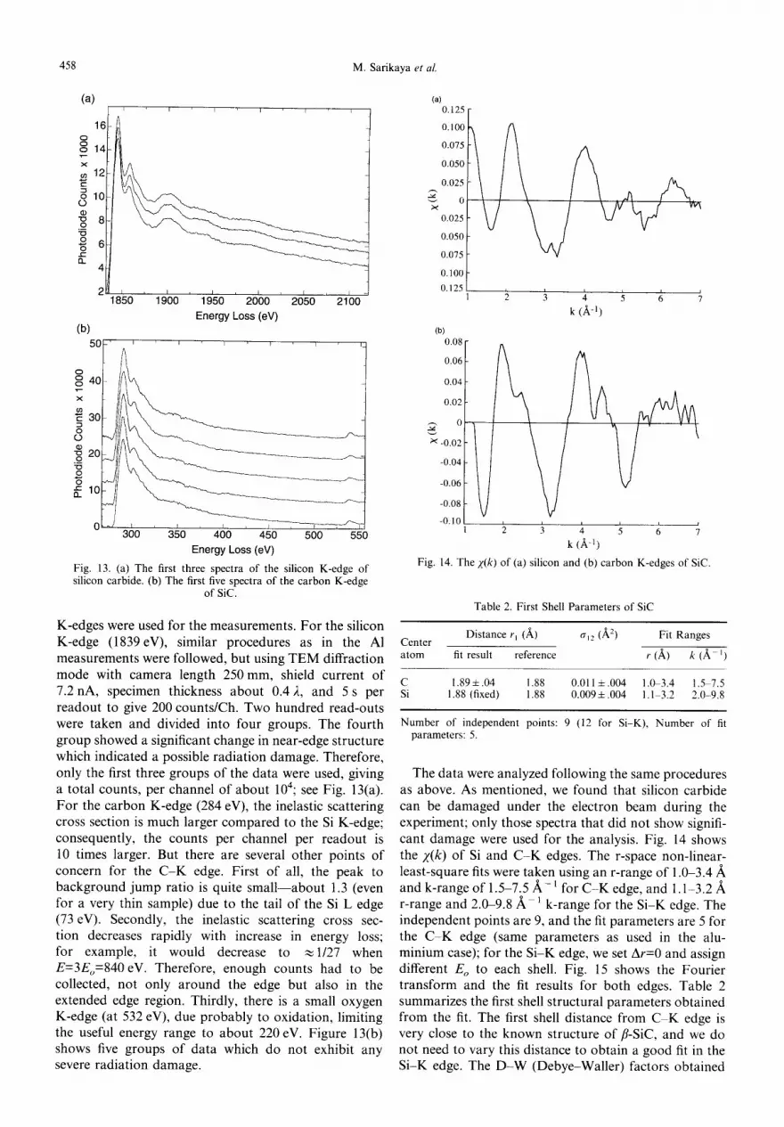
Fig. 13. (a) The first three spectra of the silicon K-edge of silicon carbide. (b) The first five spectra of the carbon K-edge

of SiC.

K-edges were used for the measurements. For the silicon K-edge (1839eV), similar procedures as in the AI measurements were followed, but using TEM diffraction mode with camera length 250mm, shield current of 7.2 nA, specimen thickness about 0.4 2, and 5 s per readout to give 200 counts/Ch. Two hundred read-outs were taken and divided into four groups. The fourth group showed a significant change in near-edge structure which indicated a possible radiation damage. Therefore, only the first three groups of the data were used, giving a total counts, per channel of about 104; see Fig. 13(a). For the carbon K-edge (284 eV), the inelastic scattering cross section is much larger compared to the Si K-edge; consequently, the counts per channel per readout is 10 times larger. But there are several other points of concern for the C - K edge. First of all, the peak to background jump ratio is quite small--about 1.3 (even for a very thin sample) due to the tail of the Si L edge (73 eV). Secondly, the inelastic scattering cross section decreases rapidly with increase in energy loss; for example, it would decrease to ~1/27 when E=3Eo=840 eV. Therefore, enough counts had to be collected, not only around the edge but also in the extended edge region. Thirdly, there is a small oxygen K-edge (at 532 eV), due probably to oxidation, limiting the useful energy range to about 220 eV. Figure 13(b) shows five groups of data which do not exhibit any severe radiation damage.

(a) 0.125

0.100

0.075 ]

0.050 [

~ 0"0250

0.025

0.050

0.075

0.100 0.125

(b) 0.08

0.06

0.04

0.02

0

~< -0.02

-O.04

-0.06

-0.08

-0.10

k (A -1)

1 Fig. 14. The z(k) of (a) silicon and (b) carbon K-edges of SiC.

Table 2. First Shell Parameters of SiC

Distance r I (fi) (712 (fi2) Fit Ranges Center atom fit result reference r (fi) k (fit 1)

C 1.89 + .04 1.88 0.011 ± .004 1.0-3.4 1.5 7.5 Si 1.88 (fixed) 1.88 0.0091.004 1.1 3.2 2.0-9.8

Number of independent points: 9 (12 for Si-K), Number of fit parameters: 5.

The data were analyzed following the same procedures as above. As mentioned, we found that silicon carbide can be damaged under the electron beam during the experiment; only those spectra that did not show significant damage were used for the analysis. Fig. 14 shows the z (k ) of Si and C - K edges. The r-space non-linear- least-square fits were taken using an r-range of 1.0-3.4 ~, and k-range of 1.5-7.5/~- l for C - K edge, and 1.1-3.2/~ r-range and 2.0-9.8/k 1 k-range for the Si-K edge. The independent points are 9, and the fit parameters are 5 for the C - K edge (same parameters as used in the aluminium case); for the Si-K edge, we set Ar=0 and assign different E o to each shell. Fig. 15 shows the Fourier transform and the fit results for both edges. Table 2 summarizes the first shell structural parameters obtained from the fit. The first shell distance from C K edge is very close to the known structure of fl-SiC, and we do not need to vary this distance to obtain a good fit in the Si-K edge. The D -W (Debye-Waller) factors obtained


(b)

X

(a) 1.0

0.8

0.6

0.4

0.2 j

ll.O I

0.6

0.5

0.4

0.3

0.2

0.1

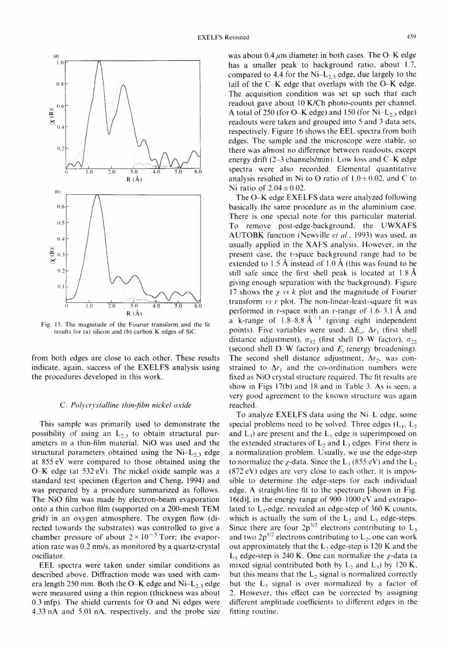
2.0 3.0 4.0 5.0 6.0 R (A)

0 1.0 2.0 3.0 4.0 5.0 6.0 R (A)

Fig. 15. The magnitude of the Fourier transform and the fit results for (a) silicon and (b) carbon K edges of SiC.

from both edges are close to each other. These results indicate, again, success of the EXELFS analysis using the procedures developed in this work.

C. Polycrystalline thin-film nickel oxide

This sample was primarily used to demonstrate the possibility of using an L2, 3 to obtain structural parameters in a thin-film material. NiO was used and the structural parameters obtained using the Ni-L2, 3 edge at 855 eV were compared to those obtained using the O K edge (at 532 eV). The nickel oxide sample was a standard test specimen (Egerton and Cheng, 1994) and was prepared by a procedure summarized as follows. The NiO film was made by electron-beam evaporation onto a thin carbon film (supported on a 200-mesh TEM grid) in an oxygen atmosphere. The oxygen flow (di- rected towards the substrates) was controlled to give a chamber pressure of about 2 x 10 -5 Torr; the evaporation rate was 0.2 nm/s, as monitored by a quartz-crystal oscillator.

EEL spectra were taken under similar conditions as described above. Diffraction mode was used with camera length 250 ram. Both the O - K edge and Ni-L2, 3 edge were measured using a thin region (thickness was about 0.3 mfp). The shield currents for O and Ni edges were 4.33 nA and 5.01 hA, respectively, and the probe size

was about 0.4/2m diameter in both cases. The O K edge has a smaller peak to background ratio, about 1.7, compared to 4.4 for the Ni-L2, 3 edge, due largely to the tail of the C - K edge that overlaps with the O - K edge. The acquisition condition was set up such that each readout gave about 10 K/Ch photo-counts per channel. A total of 250 (for O - K edge) and 150 (for Ni L2. 3 edge) readouts were taken and grouped into 5 and 3 data sets, respectively. Figure 16 shows the EEL spectra from both edges. The sample and the microscope were stable, so there was almost no difference between readouts, except energy drift (2-3 channels/rain). Low loss and C K edge spectra were also recorded. Elemental quantitative analysis resulted in Ni to O ratio of 1.0 ± 0.02, and C to Ni ratio of 2.04 + 0.02.

The O - K edge EXELFS data were analyzed following basically the same procedure as in the aluminium case. There is one special note for this particular material. To remove post-edge-background, the UWXAFS A U T O B K function (Newville et al., 1993) was used, as usually applied in the XAFS analysis. However, in the present case, the r-space background range had to be extended to 1.5 A instead of 1.0 ,~ (this was found to be still safe since the first shell peak is located at 1.8/~ giving enough separation with the background). Figure 17 shows the Z vs k plot and the magnitude of Fourier transform vs r plot. The non-linear-least-square fit was performed in r-space with an r-range of 1.6- 3.1 A and a k-range of 1 . 8 - 8 . 8 ' t (giving eight independent points). Five variables were used: AE,, Ar~ (first shell distance adjustment), al2 (first shell D W factor), a22 (second shell D W factor) and E i (energy' broadening). The second shell distance adjustment, Ar 2, was constrained to Ar I and the co-ordination numbers were fixed as NiO crystal structure required. The fit results are show in Figs 17(b) and 18 and in Table 3. As is seen, a very good agreement to the known structure was again reached.

To analyze EXELFS data using the Ni L edge, some special problems need to be solved. Three edges (L t, L 2 and L0 are present and the L 1 edge is superimposed on the extended structures of L~ and L 3 edges. First there is a normalization problem. Usually, we use the edge-step to normalize the z-data. Since the L~ (855 eV) and the L~ (872 eV) edges are very close to each other, it is impossible to determine the edge-steps for each individual edge. A straight-line fit to the spectrum [shown in Fig. 16(d)], in the energy range of 900 1000 eV and extrapolated to L3-edge, revealed an edge-step of 360 K counts, which is actually the sum of the L, and L 3 edge-steps. Since there are tbur 2p 3/2 electrons contributing to L 3 and two 2p we electrons contributing to L 2, one can work out approximately that the L 2 edge-step is 120 K and the L 3 edge-step is 240 K. One can normalize the z-data (a mixed signal contributed both by L 2 and L3) by 120 K, but this means that the L: signal is normalized correctly but the L~ signal is over normalized by a factor of 2. However, this effect can be corrected by assigning different amplitude coefficients to different edges in the fitting routine.

460 M. Sar ikaya et al.

(a)

800

0700 o o ~ 6 0 0

500

o 400 o

~ 3 0 0

~ 2 0 0

100

(c)

400

§ "~300

200

o

1oo o

-0

t r I ' ~ ' I ' I '

I

500 600 700 800 900 1000

Energy loss (eV)

I I I [

900 1000 1100 1200 1300 Energy toss (eV)

(b)

IO00F I I I l I

~8001-

600F

" ~ 4 0 0 F

~ 2 0 0 F

0 1 _ . . . L

5OO

(d1200 _

1000

o

× 800

m 600 "

o 400 -

o

200 "

-0

6()0 760 I 800

Energy loss (eV)

' ¢00 ' q i 1000

' 0' 900 1 00 1100 1200 1300 Energy loss (eV)

Fig. 16. E E L spectra of nickel oxide. (a) The first three raw spectra of oxygen K-edge and (b) the preprocessed O K-edge data, with raw data aligned, summed, and sharpened for energy resolution, and with pre-edge background, plural scattering, and Ni L-edge removed. (c) The first three group raw spectra of Nickel L2,3-edge and (d) the preprocessed L2,s-edge data with the same processing

procedure as (b) except the last step.

Table 3. Nickel oxide: oxygen K-edge fit results

Fitting parameters Given parameters

Shell # Element r (,~) ol 2 (/~2) AE,, (eV) S f n E i (eV)

1 Ni 2.08 (1) 0.026 (2) 8.5 0.9 6 0 2 O 2.95 (2) 0.025 (3) 6.5 0.9 12 0

Fit Ranges r: 1 .7-3 .1 ,~ , k: 1.8 8.8F~ - j , number of independent points: 8, number of fit parameters: 6.

A second problem is that, since both L 2 and L 3 signals are present, one needs to fit the data with contributions from both edges and shift one by the difference of the two edges, i.e. by about 17eV. Thirdly, the L 1 edge (1008 eV) is located at a position 150 eV higher from the L 3 edge and has a much smaller edge step. Ideally one should remove its contribution from the spectrum before the EXELFS analysis. However, this was not done in the present analysis; it requires detailed further work, which will be presented in a future publication (Qian et al., unpubl.). In this work, the N i -L 1 edge contribution was left in, mainly to see to what extent it would influence the analysis. Fig. 19(a) shows the x(k) vs k plot (weighted by LA). The large spectral feature around 6.5 A - 1 is the jump at the L 1 edge. Figure 19(b) shows the magni-

tude of Fourier transform. An r-space non-linear-least- square fit was performed using a r-range of 1.7-3.1 ,~, a k-range of 2 .3-10.5 ,~ J (9 independent points), six variables--A 2 (amplitude, L:-edge), AE021 (L 2 first-shell- energy-origin correction), AE022 (L 2 second-shell- energy-origin correction), Ar 1 (first-shell distance correction), a12 ( D - W factor, first-shell), a22 (D W factor, second-shell). The L3-edge amplitude was taken as one half of L 2 to compensate for the over- normalization effect explained above. The L3-edge threshold for first and second shell were obtained from AE021 and AE022 values by shifting 17 eV, and all the co-ordination numbers were fixed as the crystal structure required. Figs 19 and 20 and Table 4 show the fit results. A close examination of the results reveals that


(b)

m

(a) 3.0

2.5

2.0

1.5

2, 0.5

o

-0.5

-1.0

-I.5 2 3 4 5 6

k (A-b 8 9

1.4

1.2

I .o

0.8

0.6

0.4

0.2

o 4 6 8 10 R (A)

Fig. 17. The z(k) vs k plot (a) and Iz(r)l vs r plot (b) of oxygen K-edges from nickel oxide. The z(k) was obtained from Fig. 16 (b) by removing post-edge background and normalizing with the edge-step, z(r) is a Fourier t ransform ofz(k) using k 2 weight and 1.8-8.8 ~ 1 k-range. The fit results were also shown

(dotted line).

l

- 1 . 0 ~ J .A 1 J

2.0 3.0 4.0 5.0 6.0 7_0 8.0 9.0 k (fi, 1)

Fig. 18. The filtered z(k) obtained by back-Fourier transform- ing, using an r-window of 1.7-3.1/~ on the oxygen K-edge z(r).

The dotted line is the best fit result.

(a) 6.0

5.0

4.0

3.0

2.0

1.0

o

-1.0

2.0

-3.0

2.0 3.0 4.0 5.0 6 0 7 8.0 0.0 10.0 k ( A 4)

(b)

3.0

2.5

~, 2.(3

1.5

1.(3

0.5

0 I

2.0 4.0 6.0 8.0 10.0 R (A)

Fig. 19. The nickel oxide L2,3-edge z(k) vs k plot (a) and iz(r) vs r plot (b). Similar background removal and Fourier transformation conditions were used as in O K-edge analysis. The large feature located around 6.5 ~ l is associated with the L-edge

jump. Also shown are the best fit results (clotted).

2.0

-I.0

I I 0 21.0 41.0 6.0 8.0 10.0

k (A -1)

Fig. 20. Filtered x(k) of nickel L2.3-edge obtained by back- Fourier t ransform using an r-window of 1.7 3.1 .~. The dotted

line is the best fit result.

reasonably good fits were obtained, although there are larger misfits compared to the oxygen K-edge measurements due mainly to the existence of the Ni -L l edge. The first-shell O-Ni distance obtained from O - K edge is 2 . 0 8 + 0 . 0 1 ~ and the N i - O distance is 2.07 =L 0.02 ,~ from Ni -L edge, both agreeing very well with each other and the known structure value (Wyckoff, 1963).

D. Nanocrystalline carbonitride

A decade ago it was predicted that tetrahedral solids of low ionicity with high bulk modulus (approaching that of diamond) may be candidates for new hard materials (Cohen, 1985), such as a carbon nitride com- pound with the f l - S i 3 N 4 and other structures (Liu and Cohen, 1989; Liu and Wentzkovitch, 1994). Several groups have attempted to synthesize these covalent C N


Table 4. Nickel oxide nickel L-edge fit results


Shell # Element r (A) ~-,2 (/~2) AE,, (eV) S,, 2 n E, (eV)

1 O 2.07 (2) 0.012 (6) 0.2 1.2 6 1 2 Ni 2.92 (4) 0.015 (4) - 9 . 8 1.2 12 I

Fit Ranges r: 1.7 3.1 ~ , k: 2.3 10 .5~-~ , number of independent points: 9, number of fit parameters: 6.

(b)400 _ ,

350 - o o o 300 ' T "

x 250

e -

200 0

-o 150 ._o

o 100 o e -

a_ 5 0

0 .

I I I I " ]

i i I , I , I , P

300 350 400 450 500

Energy Loss (eV)

Fig. 21. (a) A bright field image of the sample from a region of interest containing crystalline carbonitride particles with a cubic structure in an amorphous carbonitride matrix (Sarikaya et al., submitted). (b) A characteristic EEL spectrum with C K

and N - K edges used for the analyses.

solids using various thin-film deposition techniques. (Maya et al., 1991; Niu et al., 1993; Chen et al., 1992; Fujimoto and Ogata, 1993; Yu et al., 1994; Morton et al., 1994). The material [Fig. 21(a)] used in this work was prepared by a precursor-chemistry technique heating phenyldiamonium sulfate in the presence of N 2 atmosphere and SeO 2 catalyst (Martin-Gil et al., 1995). It was recognized that the material was hard and very stable under heating and yet very light.

The electron transparent samples for TEM were prepared using an ion-beam milling with a low temperature holder, and TEM analysis was conducted using a Philips 430T TEM operated at 200 kV accelerating voltage. The analysis of the electron nanodiffraction patterns obtained from individual crystallites in various zone axis orientations results in a zinc blende structure with a lattice parameter of ao=3.52+0.05 A. FCC structure was excluded because it required a very large C-N

0.4

,-, 0.2

~ 0.0 " 4

-0.2

-0.4

-0.6

1.0 1.5. 2.0 23 3.0 3.5 4.0 4.5 5.0 5.5 6.0 k (Aq)

Fig. 22. z(k) for the carbon K-edge of carbonitride.

distance (2.49A) which is not consistent with the EXELFS result, described below, which gives the nearest C-N distance as 1.47 A.

EELS measurements were performed in TEM diffraction mode with a spot size of 50nm diameter and camera length of 250 ram. The EELS system was set to 2 mm entrance aperture and 0.5 eV/Ch dispersion. The AcqLong function was used to accumulate 105 counts/ channel at the C - K edge. Both low loss and core loss spectra were taken from sample regions having thickness less than 0.3 mfp. Fig. 21(b) shows a characteristic EEL spectrum displaying both C K and N - K edges used for the analysis. The EEL spectra obtained from several regions give a N:C ratio of 0.3 + 0.05 for a pure amorphous region and 0.4+-0.05 for the region where crystalline and amorphous phases are mixed. The volume ratio of crystalline to amorphous was estimated to be about 20%. From the estimate of the size of the particles and the relative thickness of the TEM sample used, the N:C ratio for crystalline phase was calculated to be 1.0.

EXELFS analysis was performed using the same procedures as described above. Firstly, plural scattering was removed from the raw carbon K-edge data, and then the nitrogen edge was separated and subtracted from the carbon K-edge (Qian et al., 1995b). UWXAFS analysis software was used for further analysis. To remove the post-edge background, we set E o to 290 eV (the energy scale was calibrated such that the re-feature of the edge was at 284 eV). The data was normalized by a smooth post-edge background. Fig. 22 shows z ( k ) of the C edge. The r-space non-linear-least-square fit was


0.40

0.35

• ~ 0.30 CO

0.25

o 0 . 2 0 ¢9 c

o./5

0.10 0 IJ_

0.05

I

0.0 2.0 4.0 6.0 8.0 10.0 r (A)

Fig. 23. Magnitude of the Fourier transform and the best fit result of the carbon K-edge of the carbonitride sample.

performed using a theoretical model calculated by FEFF 6.0. The theoretical model was based on the a - C 4 N 4 zincblende structure with lattice constant of 3.52 ,~ and N in the quarter diagonal positions. Accord- ing to this model, the first shell contains 4 nitrogen atoms at a distance of 1.52 A, the second shell contains 12 C atoms at a distance of 2.49 ~. The X data were square weighted. The fit r-range was set to 0.5-3.5 A and the k-range was 1.8-6.0A - l , giving 8 independent points. The fit parameters were AEo, So 2, Ar 1 (first shell distance change), Ar 2 (second shell distance change), al2 (first shell D W factor), a22 (second shell D - W factor). The two co-ordination numbers (n 1 and n2) were fixed as the model required. To compensate for the difference between theory and experiment, an energy broadening parameter E i is used and it was simply fixed to a reasonable value of 3 eV. The fit results are shown in Fig. 23 and Table 5. The first shell distance of 1.47 A agrees with the C N covalent bond radii (0.77 and 0.70/k) (Kittel, 1986), and based on this distance the lattice constant should be 3.40 ~. This value is consistent with the diffraction result (with a 3.4% difference, an error well within the accuracy, i.e. 5%, of electron diffraction technique used). The fit gives two unreason- able parameters: first shell D W factor of 0.0122,~2, which is too large, and So 2 of 0.58, which is too small due probably to the mixture of amorphous phase. The second shell contains quite a large contribution of multiple scattering which we did not include in this fitting, so the results are not as accurate as the first shell.

Based on Cohen's formula (Liu and Cohen, 1989), the new carbonitride phase having a CN composition and cubic BN structure with an C-N distance of 1.47/~ would give a bulk modulus higher than that of diamond (i.e., f~=3 .4 Mbar) (Sarikaya et al., submitted). How- ever, CN (or C 4 N 4 in the unit cell) composition would suggest that there is an extra C atom in the structure, more than that would be necessary to satisfy covalent bond formation. In the new structure, the CN composition may be satisfied with one extra electron, giving a

metallic character to the new phase, thereby decreasing the bulk modulus from the predicted value.

V. S U M M A R Y A N D C O N C L U D I N G REMARKS

We have shown that it is possible to obtain quantitative structural information from EXELFS recorded in a TEM on A1, SiC, NiO, and C4N4 samples. Because of the improvements in the transmission EELS acquisition program (Qian et al., 1995a) coupled with the benefits of a parallel detection EELS system (Krivanek et al., 1988) and the adaptation of advanced XAFS programs to EXELFS analysis (Qian el al., 1995a: Stern et a/., 1994), the quality of the data obtained from EXELFS now is comparable to that obtained at a synchrotron source. In general, one expects (Utlaut, 1981; Stern, 1982) these two techniques to give comparable quality of spectra from samples whose edges are below 1500 eV. The usual, but important, problem in the TEM (radiation damage) was not a major handicap for aluminium, but it limited analysis of the SiC sample. Radiation damage can be assessed in each sample under a given set of acquisition conditions.

EXELFS has important advantages over XAFS measurements. The EXELFS experiments can be performed in the laboratory (avoiding a clearly inconven- ient trip to a synchrotron source) if it contains the properly equipped TEM. The spatial resolution is 50 nm or less in current TEMs with LaB 6 electron sources (Newbury and Leapman, 1994) and down to subnanom- eter in dedicated STEM instruments (Batson, 1994) and new TEM's that have a field emission (FE) electron source. The spatial resolution in TEM is far superior to that of the present X-ray sources (for XAFS experiments), although the energy resolution is somewhat limited (about 1.2 eV LaB 6 and 0.5 eV in a field emission TEM) although it can be improved to less than 0.1 eV in STEM (Batson, 1994). In addition, the sample can be characterized by imaging, diffraction and nanospectros- copy techniques provided by the TEM or STEM, namely conventional and atomic resolution imaging, micro- and nano-diffraction, and EELS and energy dispersive X-ray compositional analyses, respectively. A disadvantage of EXELFS is that, lk~r dilute impurities, the large background cannot be reduced, as can be done for XAFS by detecting the signal in fluorescence instead of transmission. This limits the EXELFS technique to detecting atoms which are substantially more concentrated than the limit of XAFS detection.

Whereas it is usually stated that EXELFS contains the same information as XAFS and this statement is correct qualitatively, there are quantitative differences that need to be accounted for in order to obtain correct quantitative structure information, as discussed here. In particular, the EXELFS spectra may require a z-data renormalization to account for the different backgrounds in X-ray absorption and electron energy loss spectra (Qian et al., unpubl.).


Table 5. Carbonitride fit results (using a-C4N 4 model)


Shell # Element r (/~) al 2 (/~2) AE o (eV) S,, 2 n E i (eV)

1 N 1.47 (3) 0.012 (2) -3 .6 0.58 4 3 2 C 2.51 (10) 0.022 (10) -3 .6 0.58 12 3

VI. FUTURE PROSPECTS

We expect that it is possible to develop EXELFS so as to be a routine technique on every electron microscope equipped with a parallel recording electron energy-loss spectrometer. This opens up the possibility of applying the technique to many materials (both crystalline and amorphous), especially those with inhomogeneities on a nanometer scale, in order to obtain their local atomic structure. Some future applications may include the following:

(1) The superior spatial resolution opens up many possibilities for investigation, especially the structures of component phases in nanocrystaline structures. Furthermore, for example, it may be possible to determine the quantitative structures of interface interphases, grain boundary and twin boundary structures and defect (e.g. dislocation) core structures that require high spatial resolution. One specific example is the structure of twin boundaries in YBazCu307_ x. Upon tetragonal (normal phase) to orthorhombic phase (superconducting phase with T c ~90 K) transformation in this material, strain is developed that is accommodated by the formation of twinning on [011] planes parallel to [001] direction (e.g. Sarikaya and Stern, 1988). The local co-ordination of the ions across the twin boundary changes, causing a relaxation which ex- tends up to 20-30/~ across the twin boundary (Sarikaya et al., 1988). The twin boundary can be considered as an insulating layer and as such has a significant affect on the superconducting behavior of the material, especially the flux trapping properties. The flux line lattice that is formed in the presence of an external applied field is trapped at twin boundaries, effectively increasing the density of the supercurrent. To date, despite numerous atomic resolution electron microscopy and theoretical studies, the true structure of the twin interface has not been elucidated.

(2) Determination of short-range ordered structures, such as amorphous materials, especially within spatially restricted regions. One specific example would be the characterization of gate oxides in semiconductor devices, such as Si-based devices. The oxide film is amorphous and now extremely thin (down to a few nanometers), in response to the miniaturization of these devices. To prevent exces- sive leakage current, the composition of the gate oxides is changed, for example by introducing

(3)

(4)

nitrogen, to increase its resistivity. Under these conditions, neither the structure nor the properties of these oxides are characterized. While EELS can provide the compositional information, EXELFS can provide the local structural information using an appropriately equipped TEM. The EXELFS technique can be utilized in some crystalline samples to obtain atomic site and species-dependent information. By appropriate alignment of crystalline samples using TEMs with specimen-tilting capabilities, it is possible to produce standing electron waves which can then be used to obtain site-specific EXELFS data to distin- guish the same atom type at different crystalline sites (Spence, 1980; Spence and Tafto. 1983; Krishnan, 1990). EXELFS might also be used for orientation-dependence investigation, such as to determine different bonds, e.g. the a and ~ bonds in various materials (Leapman and Silcox, 1979). As demonstrated by us and others, EXELFS can be carried out using the K-edges; but it has less clearly been shown that EXELFS is also possible using the L and M edges, although this is a routine technique in the XAFS analysis (Okomato et al., 1991). The development of techniques for dealing with overlapping edges (such as L~ in the presence of L2,3), the effect of the use of a limited energy window in EXELFS analysis, the use and cross- correlation of mixed edges (K, L and M) in the presence of two or more elements, are all important to the wider use of this technique.

Acknowledgements--This work was supported by NEDO (Japan) and Royalty Research Funds (University of Washington).

REFERENCES

Angelini, P., Sklad, P. S., Sevely, J. C. and Husseis, D. K., 1988. Evaluation of amorphous and crystalline silicon carbide by Ex- tended Energy Loss Fine Structure (EXELFS) Analysis. In: Proc. 46th Ann. Meeting o f Electron Microsc. Soe. o f Am. San Francisco Press, San Francisco, pp. 46~467.

Batson, P. E., 1994. Atomic resolution electronic structure using spatially resolved electron energy loss spectroscopy. Proc. o f M R S Symp,, Vol. 332, M. Sarikaya, M. Isaacson, and K. Wickramasinghe (eds). Materials Research Society, Pittsburgh, PA, pp. 275-286.

Bunker, G. B., 1984. An X-ray absorption study of transition metal oxides. Ph.D. dissertation, University of Washington.

Chen, M. Y., Lin, X., Dravid, V. P., Chung, Y. W., Wong, M. S. and Sproul, W. D., 1992. Growth and characterization of C N thin films. Surg Coat. Teeh., 54-55, 360-364.

Cohen, M. L., 1985. Calculation of bulk moduli of diamond and zinc-blende solids. Phys. Rev B, 32, 7988 7991.


Cosslett, V. E., 1978. Radiation damage in the high resolution electron microscopy of biological materials: a review. J. Mierose., 113, 113 129.

Csillag, S., Johnson, D. E. and Stern, E. A., 1981. Extended energy loss fine structure studies in an electron microscope. In: EXAFS Spectroscopy Techniques and Applications, Teo, B. K. and Joy, D. C. (eds). Plenum, New York, pp. 241 254.

De Crescenzi, M., Lozzi, L., Picozzi, P. and Santucei, S., 1989. Structural determination of crystalline silicon by extended energy- loss fine-structure spectroscopy. Phys. Rev., 3912, 8409-8422.

Disko, M. M., Ahn, C. C., Meitzner, G. and Krivanek, O. L., 1988. Temperature dependence of aluminium EXELFS. In: Microheam Anal. San Francisco Press, San Francisco, pp. 47~,9.

Egerton, R. F., 1980. The use of electron lenses between a TEM specimen and an electron spectrometer. Optik, 56, 363 376.

Egerton, R. F., 1986. Electron Energy Loss Spectroscopy in the Electron Microscope. Plenum Press, New York, pp. 246 255.

Egerton, R. F. and Cheng, S. C., 1994. Characterization of an analytical electron microscope with a NiO test specimen. Ultra- microscopy. 55, 43 54.

Fujimoto, F. and Ogata, K., 1993. Formation of carbon nitride films by means of iota assisted dynamic mixing (IVD) method. Jpn. Z App/. Phys., 32, L420 423.

Glaeser, R. M., 1975. Radiation damage and biological electron microscopy. In: Physical Aspects q f Eh, ctron Microscopy and Microheam Analysis, B. M. Siegel and D. R. Beaman (eds). Wiley, New York. pp. 205 29.

Hussies, K., Zanchi, G., Sevely, J., Devaux, X. and Rousset, A., 1990. A comparative study of amorphous and crystalline alumina by EXELFS. In: Inst. Phys. Conf Ser., 98 EMAG MICRO '89. Vol. 1, pp. 75 78.

Hug, G., Phan, C. L. and Slanche, G., 1995. Some unique aspects of transmission electron microscopy and sectrometry for present and future study of intermetallic compounds. Materials Science and Engineering A, AI92-AI93, 673 684.

lsaacson, M., 1977. Specimen damage in the electron microscope. In: Principles amt Techniques o[ Eh, ctron Microscopy, M. A. Hayat ted.). Van Nostrand, New York, Vol. 7, pp. 1-78.

Johnson, D. E., Csillag, S. and Stern, E. A., 1981. Analytical electron microscopy using extended energy loss fine structure (EXELFS). Scannhtg Electr. Microsc., I, 105 115.

Kittel, C., 1986. hltrm&etion to Solid State Physics, Wiley, New York. Krishnan, K. M., 199(I. Channeling and related effects in electron

microscopy: the current status. Scanning Electron Microsc., Sup- pieing'Ill. 4, 157 170.

Krivanek, O. L., Ahn, C. C. and Keeney, R. B., 1987. Improved parallel-detection electron-energy-loss spectrometer. Ultramicro- scopy, 22, 103 110.

Kundman, M.. 1993. Itlstrt4ctions.fi~r EELS Acquisition. GATAN Inc., Pleasonton, CA, USA.

Leapman, R. D. and Cosslett, V. E., 1976. Extended fine structure above the X-ray edge in electron energy-loss spectra. J. Phys. D, 9 L, 29 32.

Leapman, R. D. and Silcox, J., 1979. Orientation dependence of core edges in electron-energy-loss spectra from anisotropic materials. Physical Review Letters, 42, 1361 1364.

Leapman, R. D. and Swyt, C. R., 1981. Electron energy-loss spectroscopy under conditions of plural scattering. In: Analytical Electron Microscopy 1981, Geiss, R. H. ted). San Francisco Press, San Francisco. pp. 164.

Leapman, R. I)., Sun, S. Q. and Andrews, S. B., 1993. Use of EELS to assess beam damage in biological microanalysis, Mieroheam AnaL, 2 (suppl.), $258 9.

Liu, A. Y. and Cohen, M. L., 1989. Prediction of new low compress- ibility solids. Science, 245, 841 842.

Liu, A. Y. and Wentzkovitch, R. M., 1994. Stability of carbon nitride solids. Phys. Rev. B, 50, 10362 10365.

Martin, J. M. and Mansot, J. L., 1991. EXELFS analysis of amorphous and crystalline silicon carbide J. Microsc., 162(1 ), 171-178.

Martin-Gil, J., Martin-Gil, F. J., Mor~in, E., Miki-Yoshida, M., Martlnez. L. and Yacaman, M., 1995. Jos6 Synthesis of low density and high hardness carbon spheres containing nitrogen and oxygen. Acta Met., 43, 1243 1247.

Maya. L., Cole, D. R. and Hagaman, W., 1991. Carbon nitrogen pyrolyzates: attempted preparation on carbon nitride. J. Amer. Ceram. Sot., 74, 1686 1688.

McMaster, W. H., Kerr Del Grande, N., Mallett, J. H. and Hubbell, J. H., 1969. Compilation of X-ray cross section, Lawrence Radi- ation Lal~oratory U('RI 50174 sec. ll, p. I.

Morton, D., Boyd, K. J., A1-Bayati, A. H., Todorov, S. S. and Rabalais, J. W., 1994. Carbon nitride deposited using energetic species: a two-phase system. Phys. Rev. Lett., 73, 118 121.

Mustre de Leon, J., Rehr, J. J., Zabinsky, S. I. and Albers, R. C., 1991. Ab initio curved-wave X-ray-absorption fine structure. Phys, Rev. B, 44, 41464156.

Newbury, D. and Leapman, R. D.. 1994. Trace analysis of nanoscale materials by analytical electron microscopy. Proc. o f M R S ,~vmp., Vol. 332, M. Sarikaya, M. lsaacson, and K. Wickramasinghe (eds.). Materials Research Society. Pittsburgh, PA, 1994, pp. 287 292.

Newvillc, M., Livin, P., Yacoby, Y., Rehr, J. and Stern, E. A., 1993. Hera-edge X-ray-absorption fine structure of Pb: A comparison of theory and experiment. Phys. Rev. B., 47, 14126 14131,

Niu. C., Lu, Y. Z. and Lieber, C. M., 1993. Experimental realization of the covalent solid carbon nitride. Science. 261,334 336.

Okomato, J. K., Ahn, C. C. and Fultz, B., 1991. EXELFS analysis of AI K, Fe L:.> and PdM4,~ edges. In: Microheam Analv.~is, 1991. San Francisco Press, San Francisco, pp. 273 276.

Qian, M., Sarikaya, M. and Stern, E. A., 1993a. Acquisition of EELS spectra for high-resolution spectroscopy. In: PJoceedin~,s q f the 51si Annual ~Ieeting o / Mieroscop.t' Society ~,'t America. San Francisco Press, San Francisco, pp. 578 579.

Qian, M., Sarikaya. M. and Stern, E. A.. 1993b. EXELFS revisited: an improved data analysis technique. In: Proceedhlgs q f the 51st Annual Meeting o/Microscopy Society ¢~/,4nwric,:t. Sun Francisco Press, San Francisco, pp. 584 585.

Qian, M., Sarikaya, M. and Stern, E. A., 1995a. Development of the EXELFS technique for high accuracy structural information. Ultramicrosc~q~y. 59, 137 147.

Qian, M.. Sarikaya, M. and Stern, E. A., 1995b. Removing edge overlapping for maximum usage of EXELFS signal. In: Proceed- h~g.s ~!/ the 53rd Ann ual Meeting o/Microscopy So~qety ol A nzeri~'a. San Francisco Press, San Francisco, pp. 3(/2 303.

Rehr, J. J.. Albers. R. C., Zabinsky, S. I., 1992. High-order multiple- scattering calculations of X-ray absorption fine structure. Phys. Rev. Lett., 69, 3397 3400.

Rehr, J. J., Mustre de Leon, J., Zabinsky. S. 1. and Albers. R. C.. 1991. Theoretical X-ray absorption fine structure standards. ,I. Am. (Tu'm. Sot., 113, 5135 5140.

Reimer, L., 1975. Review of radiation damage problem of organic specimens in electron microscopy. In: Physical Aspects o/Eleetron Microseopy amt Mieroheam Anulvsis, B. M. Siegel and D. R. Beaman (eds). Wiley. New York, pp. 231 245.

Sarikaya. M. and Stern. E. A., 1988. Twining in YBa~Cu~O, ~. Plow. Rev. B., 37(16), 9373 9381.

Sarikaya, M., Kikuchi, R. and Aksay. I. A., 1988. Structure and formation of twinning in YBa~Cu~O: ,. Ph.t'sica C, 1522, 161 17(I.

Sarikaya. M. ted.), 1992. Resolution in the Microscope, Ullramicro- scnpy, 47, 1306.

Sarikaya, M., Qian, M., Stern, E. A., 1995. Copyrighted UWEXELFS 1.0 software. Information regarding the UWEXELFS 1.0 may be obtained from M. Sarikaya, University of Washington.

Sayers. D. E., Stern, E. A. and Lytle, F. W., 1971. New technique for investigating noncrystalline structures: Fourier analysis of the extend X-ray-absorption fine structure. Phys. R(,v, Lett.. 27, 1204 1207.

Serin, V., Zanchi, G. and Sevely, J., 1992. EXELFS as a structural tool for studies of low z-elements. Microsc. Microana/. Microslruct., 3, 201 212.

Spence, J. C. H., 1980. The use of characteristic-loss energy selected electron diffraction patterns for site symmetry determination. Optik. 57, 451 456.

Spence, J. C. H. and Tafto, J., 1993. J. Microsc., 131t, 147 154. Stern, E. A., 1982. Comparison between electrons and X-rays for

structure determination. Optik, 61, 45 51. Stern, E. A. and Heald, W. M., 1983. Basic principles and appli-

cations of EXAFS. In: Handbook on Synchrotron Radiation,, Vol. 1, Ch. 10. North Holland, Publisher, New York. pp. 955 1014.

Stern, E. A. et al., 1995. The copyrighted UWXAFS 3.0 software. Information regarding this software may be obt'tined fi'om E. A. Stern, University of Washington.

Stern, E. A.. Qian, M. and Sarikaya, M., 1994. Spatially Resolved Local Atomic Structure From EXELFS. Proc. o f M R S Syrup., Vol. 332, Sarikaya, M., Isaacson, M. and Wickramasinghe, K. (edsl. Materials Research Society,. Pittsburgh, PA, pp. 3 14.


Utlaut, M., 1981. A comparison of Electron and Photon Beams for Obtaining Inner Shell Spectra. EXAFS Speetroscopy Techniques and Applications, B. K. Tao and D. C. Joy (eds). Plenum, New York, pp. 255 267.

Wyckoff, R. W. Crystal Structures. Interscience Publication, New York, NY, 1963.

Yu, K. M., Cohen, M. L., Hailer, E. E., Hansen, W. L., Liu, A. Y. and Wu, I. C., 1994. Observation of crystalline C3N 4. Phys. Rev. B., 49, 5034-5037.

Zeitler, E., 1979. Radiation damage in beam-sensitive materials. In: Developments in Electron Microscopy and Analysis 1979, H. J. Goringe (ed.). Inst. Phys. Conf. Ser. No. 61, I. O. P. Bristol, pp. 1-6.

Documents

EXELFS revisited