Embed Size (px)
Citation preview

Seediscussions,stats,andauthorprofilesforthispublicationat:https://www.researchgate.net/publication/47865302
TheCasimirspectrumrevisited
ARTICLEinJOURNALOFMATHEMATICALPHYSICS·DECEMBER2010
ImpactFactor:1.24·DOI:10.1063/1.3614003·Source:arXiv
READS
13
3AUTHORS,INCLUDING:
CarlosHerdeiro
UniversityofAveiro
119PUBLICATIONS2,008CITATIONS
SEEPROFILE
JaimeEduardoSantos
UniversityofMinho
27PUBLICATIONS282CITATIONS
SEEPROFILE
Availablefrom:CarlosHerdeiro
Retrievedon:04February2016

arX
iv:1
012.
1140
v1 [
quan
t-ph
] 6
Dec
201
0
The Casimir spectrum revisited
Carlos A.R. Herdeiro,1, 2, ∗ Marco O.P. Sampaio,2, † and Jaime E. Santos2, 3, ‡
1Departamento de Fısica da Universidade de Aveiro,
Campus de Santiago, 3810-183 Aveiro, Portugal.2Centro de Fısica do Porto — CFP, Departamento de Fısica e Astronomia,
Faculdade de Ciencias da Universidade do Porto — FCUP,
Rua do Campo Alegre, 4169-007 Porto, Portugal.3Max Planck Institute for the Physics of Complex Systems,
Noethnitzer Str. 38, D-01187 Dresden, Germany.
We examine the mathematical and physical significance of the spectral density σ(ω) introducedby Ford in [1], defining the contribution of each frequency to the renormalised energy density ofa quantum field. Firstly, by considering a simple example, we argue that σ(ω) is well defined,in the sense of being regulator independent, despite an apparently regulator dependent definition.We then suggest that σ(ω) is a spectral distribution, rather than a function, which only producesphysically meaningful results when integrated over a sufficiently large range of frequencies and witha high energy smooth enough regulator. Moreover, σ(ω) is seen to be simply the difference betweenthe bare spectral density and the spectral density of the reference background. This interpretationyields a simple ‘rule of thumb’ to writing down a (formal) expression for σ(ω) as shown in anexplicit example. Finally, by considering an example in which the sign of the Casimir force varies,we show that the spectrum carries no manifest information about this sign; it can only be inferredby integrating σ(ω).
PACS numbers: 11.10.Gh, 03.70.+k
I. INTRODUCTION
Can one assign a frequency spectrum to the finiteCasimir energy? This question was first posed by Fordin [1] where such frequency spectrum, henceforth dubbedCasimir spectrum, was considered for two examples: amassless scalar field in R × S1 and R
3 × S1. The spec-trum is encoded in a spectral density σ(ω) which mustobey two obvious criteria: i) integrated over all frequen-cies it must yield the renormalised vacuum energy
ρren ≡ 〈0|T00|0〉ren =1
2π
∫ +∞
0
σ(ω)dω , (1.1)
where the quantum field has energy momentum tensorTµν in a space-time admitting a globally time-like Killingvector field ∂/∂x0 ; ii) it should not depend on the renor-malisation/regularisation procedure. Whereas the firstcriterion is easy to check, the second one seems hard toprove. Indeed, the very definition of the spectral den-sity introduced in [1] was based on a specific regular-isation/renormalisation scheme, namely point splitting.This definition is
σ(ω) = 2
∫ +∞
−∞
〈0|T00(τ)|0〉reneiωτdτ , (1.2)
where τ is a point-splitting regulator along the time com-ponent. We shall show in Section IID, however, that
∗ [email protected]† [email protected]‡ [email protected]
this definition, albeit apparently tied to point-splittingregularisation, is quite general, and thus, that in this re-spect the Casimir spectrum is well defined. From thesame analysis we shall learn that renormalised spectraldensity σ(ω) is simply the difference between the barespectral density and the spectral density of the refer-ence background. This provides us with an immediatetool to write down a formal expression for it. But if anappropriate regulator is not included, this expression ismeaningless. Moreover, we shall see that even with anappropriate regulator, only the integration of this spec-tral density carries some physical information, and onlyif the integration extends through a sufficiently large fre-quency interval. Thus one should regard σ(ω) as a spec-tral distribution, rather than a function.
As another test on the physical information carried bythe Casimir spectrum, we analyse the case of a scalarfield, with mass parameter and coupling to the curva-ture, in an Einstein Static Universe. It has been shownin [2, 3], that the renormalised energy momentum ten-sor associated to the vacuum fluctuations may obey orviolate the strong energy condition, depending on thevarious parameters, therefore potentially sourcing repul-sive gravity. Our analysis shows, however, than no hintabout the sign of the Casimir force may be obtained,in this case, from the Casimir spectrum. Thus, althoughwe find that the Casimir spectrum is mathematically welldefined, we find no evidence about it carrying more phys-ical information than that carried by the Casimir energyitself.
This paper is organised as follows. In section 2 westart by reviewing the computation of the Casimir spec-trum for a massless scalar field in R× S1, discussing the

2
generality of the definition (1.2) as well as its interpre-tation and physical content. In section 3 we discuss theCasimir spectrum on the Einstein Static Universe, wherewe show that no noticeable difference is seen when thegravitational effect of the Casimir energy varies from at-tractive to repulsive. In Appendix A we consider anotherexample, a scalar field in R
3 × S1, that confirms the ar-guments and interpretation provided in Section 2.
II. RECONSIDERING R× S1
We start by reconsidering the case of a massless scalarfield on a 2-dimensional space-time with one periodicspace-like direction, of length L. The space-time is thenR×S1. We shall review the computation of the spectrumusing a weight function [1, 4] and then compute it usingpoint-splitting.
A. Weight functions
The regularised energy density (with a weight func-tion) is
ρx0,m =1
2L
+∞∑
n=−∞
ωnW (ωn)x0,m , (2.1)
with ωn = 2π|n|/L. We can apply the Abel-Plana for-mula as long as the condition
limy→∞
e−2πy |G(x ± iy)| = 0 ,
is satisfied (where G(n) is the function inside the sum).The choice of weight function in [1] is
W (2πx/L)x0,m =
(
2m
x0
)2m+1x2m
(2m)!e−2mx/x0 , (2.2)
where m ∈ N. This clearly obeys the conditions of appli-cability of the Abel-Plana formula. Applying the formulawe get
ρx0,m =1
2π
∫ +∞
0
ωW (ω)dω
− 2π
L2
∫ +∞
0
t (W (2πit/L) +W (−2πit/L))
e2πt − 1dt . (2.3)
The first term renormalises the cosmological constantsince it is a background independent constant. The sec-ond term is identified as the spectral function. Note thatthe weight functions (2.2) were chosen as to become deltafunctions δ(x−x0) in the large m limit, which when inte-grated over x0 give 1. Also, x0 = Lω0/(2π); the spectralfunction so defined is then normalised to give the correct
energy density when integrated with this differential. Re-placing by the explicit form of the weight function we get
σm(x0) =2π(−1)m+1
L2(2m)!
(
2m
x0
)2m+1
×
×∫ +∞
0
t2m+1
(
e2mitx0 + e−
2mitx0
)
e2πt − 1dt . (2.4)
If we expand the denominator as a geometric series andperform the integrals, then the sums can be identified asHurwitz zeta functions and the final expression coincideswith that of [4]:
σm(x0) =(−1)m+1(2m+ 1)
L2
(
m
πx0
)2m+1
×[
ζH
(
2m+ 2, 1− im
πx0
)
+ ζH
(
2m+ 2, 1 + im
πx0
)]
.
(2.5)
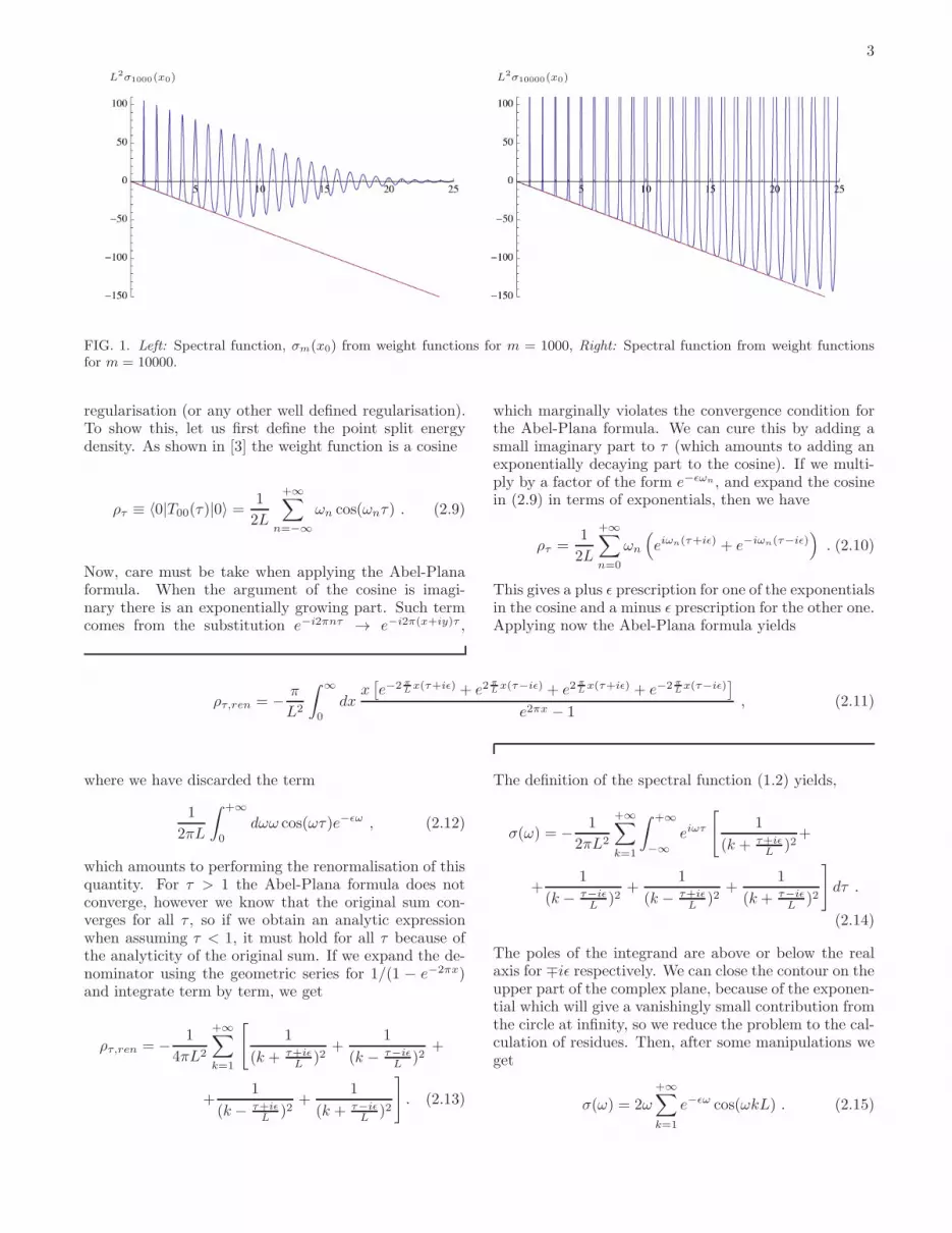
The plot in Fig. 1 reveals that in the limit of largem the spectrum becomes just the difference between lo-calised delta functions and a straight line with negativeslope which matches the flat space spectrum. Indeed,re-writing the energy density as
ρ =1
2L
+∞∑
n=−∞
ωn =
∫ +∞
0
dωω1
2L
+∞∑
n=−∞
δ(ω − ωn)
=1
L
∫ +∞
0
dωω
+∞∑
n=1
δ(ω − ωn) (2.6)
and subtracting the flat space contribution (assuming amassless field), we get
ρren =1
L
∫ +∞
0
dωω
+∞∑
n=1
δ(ω − ωn)−1
2
∫ +∞
−∞
dk
2πωk
=
∫ +∞
0
dωω
(
+∞∑
n=1
1
Lδ(ω − ωn)−
1
2π
)
. (2.7)
Thus, in this simple case, it is clear that the spectraldensity is really
σ(ω) = ω
(
2π
+∞∑
n=1
1
Lδ(ω − ωn)− 1
)
. (2.8)
The terms in parenthesis show that the continuum fre-quencies have a negative uniform weight, whereas thediscrete frequencies have a delta function uniform weight.The difference corresponds exactly to the limit ofm → ∞in Fig. 1.
B. Point Splitting
The first form of the spectrum obtained in the previoussection, depended on a particular choice of weight func-tion. But the same result is obtained with point splitting
3
L2σ1000(x0) L2σ10000(x0)
FIG. 1. Left: Spectral function, σm(x0) from weight functions for m = 1000, Right: Spectral function from weight functionsfor m = 10000.
regularisation (or any other well defined regularisation).To show this, let us first define the point split energydensity. As shown in [3] the weight function is a cosine
ρτ ≡ 〈0|T00(τ)|0〉 =1
2L
+∞∑
n=−∞
ωn cos(ωnτ) . (2.9)
Now, care must be take when applying the Abel-Planaformula. When the argument of the cosine is imagi-nary there is an exponentially growing part. Such termcomes from the substitution e−i2πnτ → e−i2π(x+iy)τ ,
which marginally violates the convergence condition forthe Abel-Plana formula. We can cure this by adding asmall imaginary part to τ (which amounts to adding anexponentially decaying part to the cosine). If we multi-ply by a factor of the form e−ǫωn, and expand the cosinein (2.9) in terms of exponentials, then we have
ρτ =1
2L
+∞∑
n=0
ωn
(
eiωn(τ+iǫ) + e−iωn(τ−iǫ))
. (2.10)
This gives a plus ǫ prescription for one of the exponentialsin the cosine and a minus ǫ prescription for the other one.Applying now the Abel-Plana formula yields
ρτ,ren = − π
L2
∫ ∞
0
dxx[
e−2 πLx(τ+iǫ) + e2
πLx(τ−iǫ) + e2
πLx(τ+iǫ) + e−2 π
Lx(τ−iǫ)
]
e2πx − 1, (2.11)
where we have discarded the term
1
2πL
∫ +∞
0
dωω cos(ωτ)e−ǫω , (2.12)
which amounts to performing the renormalisation of thisquantity. For τ > 1 the Abel-Plana formula does notconverge, however we know that the original sum con-verges for all τ , so if we obtain an analytic expressionwhen assuming τ < 1, it must hold for all τ because ofthe analyticity of the original sum. If we expand the de-nominator using the geometric series for 1/(1 − e−2πx)and integrate term by term, we get
ρτ,ren = − 1
4πL2
+∞∑
k=1
[
1
(k + τ+iǫL )2
+1
(k − τ−iǫL )2
+
+1
(k − τ+iǫL )2
+1
(k + τ−iǫL )2
]
. (2.13)
The definition of the spectral function (1.2) yields,
σ(ω) = − 1
2πL2
+∞∑
k=1
∫ +∞
−∞
eiωτ
[
1
(k + τ+iǫL )2
+
+1
(k − τ−iǫL )2
+1
(k − τ+iǫL )2
+1
(k + τ−iǫL )2
]
dτ .
(2.14)
The poles of the integrand are above or below the realaxis for ∓iǫ respectively. We can close the contour on theupper part of the complex plane, because of the exponen-tial which will give a vanishingly small contribution fromthe circle at infinity, so we reduce the problem to the cal-culation of residues. Then, after some manipulations weget
σ(ω) = 2ω
+∞∑
k=1
e−ǫω cos(ωkL) . (2.15)

4
Note that keeping the convergence factor with the ǫ iscrucial to induce the correct contour in the integration.We can integrate the spectral function (2.15) to checkthat we recover the Casimir energy
ρren =
∫ +∞
0
dω
2π2ω
+∞∑
k=1
e−ǫω cos(ωLk)
=1
πL2
+∞∑
k=1
ǫ2 − k2
(ǫ2 + k2)2→ − π
6L2. (2.16)
Using the Fourier series representation of the periodicrepetition of the delta function one can show that the sum(2.15), with ǫ → 0, is equivalent to (2.8). Thus, usingpoint-splitting we recover the spectral function obtainedin the previous subsection using a weight function.
C. Spectral function or spectral distribution?
The natural question is: does σ(ω) carry some extraphysical content, as compared to the energy density? Orin other words: is the spectral function σ(ω) meaningfulonly when integrated over the whole frequency range, orcan one assign a physical value to an integration over an
interval,∫ ω0+∆ω
ω0σ(ω)dω ?
To answer this question we can integrate σ(ω) in (2.15)convoluted with some other functions. For example wecan take functions which are non-zero only in regionswith only one delta function contribution. For exampleif we choose, for j ∈ N
fj(ω) =
1 , (2πj − π)/L < ω < (2πj + π)/L0 , otherwise
,
(2.17)then, using (2.15),
∫ +∞
0
fj(ω)σ(ω)dω
2π= 0 . (2.18)
This is exactly what we obtain from integrating fj(ω)with the delta distribution centred at 2πj/L, and sub-tracting the result from integrating fj(ω) with ω/(2π),cf. (2.8). But integration over the first (remaining) inter-val yields
∫ π/L
0
σ(ω)dω
2π= − π
4L2, (2.19)
rather than −π/6L2, which is the renormalised energydensity. This is a consequence of manipulating divergentinfinite sums without regularising them. Of course, ifone keeps the convergence factor e−ǫω in (2.16), and in-tegrates again over the full range of frequencies, one willobtain the correct result. This makes clear that the spec-tral function σ(ω) is only meaningful when regularised.What if we include a regulator in σ(ω)? Does the spec-
tral function then acquire a physical meaning when inte-grated over a compact range of frequencies (as opposed
to all frequencies)? A hint to answer this question comesfrom work on semi-transparent boundaries [5]. Therein,the Casimir force is given by a difference of pressures in-side the plates and outside the plates, computed fromscattering of modes inside and outside the plates. Insuch computation there is a physical coefficient playingthe role of a reflection factor, which becomes the physicalregulator. A related idea was discussed in [6].Assuming that the spectral function has a physical
meaning, we could think about integrating it over a fi-nite range of frequencies, to mimic the situation of trans-parency in the remaining range of frequencies. Let us firstconsider this is done in a sharp way, i.e. by introducinga Heaviside step function H(x) cut-off:
F1(q, ω0) ≡∫ ω0
0
dω
2πσ(ω)H(q − ω) . (2.20)
In Fig. 2 we plot F1(q, ω0). It oscillates wildly and itdoes not converge to the renormalised energy density inthe limit ω0 → ∞.However, we can introduce a smoother regulator, as
we would expect in an actual physical situation such asin [5]. Using the exponential cut-off e−ǫω, so that we caninterpret q = 1/ǫ as the scale at which the theory is UVcompleted; then consider
F2(q, ω0) ≡∫ ω0
0
dω
2πσ(ω)e−ω/q . (2.21)
This function is plotted in Fig. 3. It can be seen thatthe integrated value of the spectral function now ap-proaches asymptotically the Casimir energy density ofthe system. Thus, for the spectral function to be phys-ical, a regulator that suppresses the UV frequencies iscrucial and it should correspond to an actual physicalcut-off of the theory. It is a remarkable fact that theCasimir force does not depend on the details of such regu-lator, but only on the existence of a high energy “smoothenough” damping of the modes.
D. Interpretation of σ(ω) and computational
shortcut
Inspired by the previous example, and since the defini-tion of the spectral density (1.2) is not derived from firstprinciples, let us reconsider it starting from the (bare)energy density formula. Keeping the convergence fac-tor e−ǫωn
ρ =1
2L
+∞∑
n=−∞
ωne−ǫωn
=
∫ +∞
−∞
dωω1
2L
+∞∑
n=−∞
δ(ω − ωn)e−ǫωn
=
∫ +∞
0
dωω
L
+∞∑
n=1
(δ(ω − ωn) + δ(ω + ωn)) e−ǫωn .(2.22)

5
L2F1(100, ω0) L2F1(1000, ω0)
FIG. 2. Integral of the spectral function regularised with a step function at q, up to an energy ω0 Left: F1(100, ω0), Right:F1(1000, ω0).
L2F2(100, ω0)
-
L2F2(1000, ω0)
-
FIG. 3. Integral up to an energy ω0, of the spectral function regularised with an exponentially decaying function Left:
F2(100, ω0), Right: F2(1000, ω0). The asymptotic result is indicated by the horizontal line in the zoomed plots on the right.
Observe that the second delta function does not con-tribute. From this we see that the bare spectral functionwith the normalisation (1.1) is
σbare =2π
L
+∞∑
n=1
ωn (δ(ω − ωn) + δ(ω + ωn)) e−ǫωn .
(2.23)
If we replace here the Fourier expansion of the delta func-tion
σbare =
+∞∑
n=1
∫ ∞
−∞
dτ
Lωn
[
eiτ(ω−ωn) + eiτ(ω+ωn)]
e−ǫωn
=2
L
∫ ∞
−∞
dτeiτω+∞∑
n=1
ωn cos(τωn)e−ǫωn
(2.9)= 2
∫ ∞
−∞
〈0|T00(τ)|0〉eiτωdτ . (2.24)

6
So the fact that the spectral function is the Fourier trans-form of the point split energy density is not restricted to
using point splitting regularisation; indeed we have notused it in this argument. This expression appears simplyfrom Fourier expanding the delta functions.The lesson from this example is that the renormalised
spectral density σ(ω) is simply the difference between thebare spectral density above and the spectral density ofthe reference background. In Appendix A we show thatthis simple ‘rule of thumb’ yields the correct result forthe computation of the spectral density in another wellknown example: a massless scalar field in R
3 × S1.
III. APPLICATION TO R× S3
We will now ask another question concerning the phys-ical content of the spectral function: does it carry anyhint concerning the sign of the Casimir force? It is wellknown that the Casimir force can either be attractive orrepulsive depending on details of the geometry, topologyor boundary conditions that originates it (see [7] for areview). What determines the sign of the Casimir forceis still an open problem.This question is particularly relevant since Casimir
forces are a dominant interaction at the nanometer scaleand therefore of relevance for the construction of nano-devices. Repulsive Casimir forces (see e.g. [8, 9]) couldallow quantum levitation and therefore avoid collapseand permanent adhesion between nearby surfaces, whichis a problem for microelectromechanical systems. More-over, repulsive Casimir forces are not just a theoreticalpossibility since there is some experimental evidence [10–12].In order to tackle this question we shall consider an
example where it has been shown that the effect of theCasimir energy can change from attractive to repulsive,when one varies the parameters of the system: a scalarfield with a mass parameter and a coupling to the Ricciscalar in the Einstein Static Universe (ESU) [2, 3].
A. Setup
We consider a scalar field theory in the 3 + 1 dimen-sional ESU
ds2ESU = −dt2 +R2dΩS3 . (3.1)
The Ricci scalar of the geometry is R = 6/R2, where theradius of the universe is R. This geometry is perturbedby the quantum vacuum fluctuations of a real scalar fieldwith action
SΦ =
∫
d4x√−g
(
−1
2∂αΦ∂
αΦ− 1
2µ2Φ2 − 1
2ξRΦ2
)
.
(3.2)We are interested in analysing the energy spectrum ofthe quantum field in a vacuum state (with respect to
the global timelike Killing vector). This can be done bysolving the classical equations of motion for the scalarfield, then quantising the theory and finally computingexpectation values of observables in such a state. Sincewe are interested in the energy density we have to lookat the expectation value of the energy momentum tensor
TΦµν = ∂µΦ∂νΦ+ ξ (Rµν −DµDν)Φ
2+
+ gµν
(
2ξ − 1
2
)
[
∂αΦ∂αΦ+ (µ2 + ξR)Φ2
]
. (3.3)
This procedure was explained in detail in [2, 3], so herewe simply summarise the main results needed for ourstudy in 3 + 1 dimensions. The scalar field is expandedin the Heisenberg picture using the eigenmodes
φα(t, x) =1√2ωℓ
e−iωℓtYα(x) , (3.4)
where α = ℓ,mR,mL : ℓ ∈ N0∧−ℓ < mL,mR < ℓ ∈ Z,Yα(x) are the hyperspherical harmonics and x denotesthe angular coordinates on S3. The eigenfrequencies are
ωℓ =√
k2 + a2 , (3.5)
with
k ≡ ℓ+ 1
R, a2 ≡ µ2 +
6ξ − 1
R2. (3.6)
The Vacuum Expectation Value (VEV) of any compo-nent of TΦ
µν can be expressed in terms of 〈0| (TΦ)00 |0〉using the conservation of energy. Its bare value is for-mally divergent, so it requires a regularisation procedurefollowed by renormalisation which we address in the nextsection.
B. The spectrum on the ESU from a generic
regularisation
As seen in [3], the renormalisation of the energy mo-mentum tensor on the ESU can be performed just byspecifying some generic physical properties for the UVcompletion of the theory, encoded in a generic regulator.Then the regularised energy density is simply
ρ0 =1
2V
+∞∑
ℓ=0
dℓωℓ g (γLωℓ) , (3.7)
where V is the volume of S3, g is a generic regularisationfunction that goes to 1 in the infrared, γ ≪ 1 is theregularisation parameter, L is the typical length scale ofthe system, and the degeneracy of the modes is
dℓ = (ℓ+ 1)2 . (3.8)
Using the Abel-Plana formula ρ0 can be re-written as
ρ0 =R3
2V
∫ +∞
ωmin
dω√
ω2 − a2ω2g(γLω) + ρren , (3.9)

7
where ωmin = a if a2 > 0, otherwise ωmin = 0. The firstintegral is the quantity that is discarded and containsall the divergences that renormalise various gravitationalcouplings. In fact, to obtain the spectrum, this is exactlythe quantity that we need to subtract from the discretespectrum. This can be written as
ρdiv =
∫ +∞
0
dω
2π
πR3
V
√
ω2 − a2ω2g(γLω)θ(ω − ωmin) .
(3.10)So now, using our ‘rule of thumb’ we can just subtractthe integrand from the discrete spectrum to obtain thespectrum
σESU =πω
V
[
R2(ω2 − a2)+∞∑
ℓ=0
δ (ω − ωℓ)−
−R3ω√
ω2 − a2θ(ω − ωmin)]
g(γLω) . (3.11)
Once again we can define the integral of the spectrumup to an energy ω0 and make the plot for various a. Iffor example we take the massless case, then we can showthat for this case, the quantity ρ+ 3p, which determinesif the strong energy condition is obeyed, simplifies to
ρ+ 3p = 2ρ , (3.12)
so that it is simply the sign of ρ that determines if thegravitational effect of the Casimir energy is attractive(ρ > 0) or repulsive (ρ < 0). The change from a repulsiveto an attractive effect can be obtained by varying a2R2,or equivalently ξ [2, 3]. For convenience we define theintegrated spectrum
F (q, a2, ω0) = 2R4V (3)
∫ ω0
0
σESU (ω)dω
2π, (3.13)
with g(γLω) = e−ω/q. Some examples are exhibited inFig. 4, for which one varies a2 such that the effect variesfrom attractive to repulsive. The conclusion is that thereis no manifest qualitative change in the spectrum andthe variation in character of the Casimir force can onlybe observed upon integration of the spectral function.Thus, it seems that again, the Casimir spectrum carriesno added value, relatively to the Casimir energy density,in terms of physical content.
IV. CONCLUDING REMARKS
In this paper we have reconsidered the Casimir spec-trum, defined in [1]. Based on the study of three dif-ferent examples (two of which had already been consid-ered in [1]) we have reached the following conclusions:1) despite the apparent regularisation scheme dependentdefinition (1.2), the Casimir spectrum is mathematicallywell defined, in the sense of being scheme independent;2) a simple interpretation for the spectrum is provided:
the renormalised spectral density σ(ω) is simply the dif-ference between the bare spectral density and the spec-tral density of the reference background. This providesus with a simple rule to write down a formal expressionfor the spectrum; 3) the spectrum should, however, befaced as a distribution, rather than a function. That is,it is not differentiable but it is integrable, and also it isonly physically meaningful when integrated over a suf-ficiently large range of frequencies, with a high energysmooth enough regulator. Thus we find no evidence thatthe spectrum carries an added value, in terms of phys-ical content, relatively to the energy density itself. Inparticular, by considering an example where the effectof the Casimir energy can vary its character from repul-sive to attractive, we found that there is no manifestimprint of this change of character in the properties ofthe spectrum. We note that a possible relation betweenthe Casimir spectrum and the sign of the Casimir forcewas previously discussed in [6].
ACKNOWLEDGEMENTS
We would like to thank L. Ford for comments on a draftof this paper and Goncalo Dias for collaboration duringthe early stages of this work. We would also like to thankManuel Donaire and Filipe Paccetti for discussions. M.S.is supported by the FCT grant SFRH/BPD/69971/2010.J.E.S. would like to thank the MPIPkS for support inthe framework of its Visitors Program. This work is alsosupported by the grant CERN/FP/109306/2009.
APPENDICES
Appendix A: Check for S1× R
3
In [1] the spectrum of the Casimir effect, for a masslessscalar field in flat spacetime, with one periodic spatialdirection was computed using Green’s functions. In thisappendix we show that the shortcut suggested in SectionIID yields the same result, which is also checked by usingpoint-splitting regularisation.In this case, due to the boundary conditions, the field
expansion is
Φ =
∫
d2k∑
ℓ
[
aℓ(k)φℓ(k, xµ) + a†ℓ(k)φ
∗ℓ (k, x
µ)]
,
(A1)where the creation and annihilation operators obey stan-dard harmonic oscillator commutation relations, and
φℓ(k, xµ) =
1
2π√
2ωℓ,kLe−iωℓ,kt+i( 2πℓ
Lx+kyy+kzz) , (A2)
with
ωℓ,k =
√
(
2πℓ
L
)2
+ k2 . (A3)

8
F (1000, 1, ω0)
-
F (1000,−0.92, ω0)
-
F (1000,−a20, ω0)
-
F (1000,−0.72, ω0)
-
F (1000, 0, ω0)
-
FIG. 4. Integral up to energy ω0, of the spectral function regularised with an exponentially decaying function, for variouschoices of a2. The asymptotic result is indicated by the horizontal line in the zoomed plots (right). Note that −a2
0 is the valuefor which the renormalised energy density vanishes; which can be seen on the corresponding zoomed plot up to an error of 10−4.

9
The first step is to compute the vacuum expectation value of the regularised energy density from the energymomentum tensor
〈0|T00(x − x′) |0〉 ≡ 1
2〈0|∂0Φ∂0′Φ′ +
1
2∂α′Φ′∂αΦ + x ↔ x′ |0〉
=1
2L
∫
d2k
(2π)2
+∞∑
ℓ=−∞
ωℓ,k cos
[
ωℓ,k(t− t′)− 2πℓ
L(x− x′)
]
ei(ky(y−y′)+kz(z−z′)) , (A4)
where we have used the field expansion and the canonicalcommutation relations for the creation and annihilationoperators.Taking time separation only τ = t−t′, and introducing
a convergence factor to make sure the sum converges wehave
〈0|T00(τ) |0〉 =1
2L
∫
d2k
(2π)2
+∞∑
ℓ=−∞
ωℓ,k cos (ωℓ,kτ) e−ǫωn .
(A5)Before applying the Abel-Plana formula let us use the
insight of Section II D to anticipate the answer (since thespectrum was seen as a difference between the bare spec-tral density and the flat space spectral density). The barespectral density is obtained by inserting a delta function
ρ =1
2L
∫
d2k
(2π)2
+∞∑
ℓ=−∞
ωℓ,k (A6)
=
∫
dω
2π
1
2L
∫
d2k
(2π)2
+∞∑
ℓ=−∞
ωℓ,k2πδ(ω − ωℓ,k) .
So
σbare(ω) =1
2L
∫
d2k
(2π)2
+∞∑
ℓ=−∞
ωℓ,k2πδ(ω − ωℓ,k)
=1
2L
+∞∑
ℓ=−∞
∫ +∞
0
dkkωℓ,kδ(ω − ωℓ,k)
=ω2
2L
(
1 + 2
+∞∑
ℓ=1
θ(ωL− 2π|ℓ|))
. (A7)
The flat limit spectrum is clearly
σflat(ω) =ω3
2π, (A8)
so we expect the spectrum to be the difference be-tween (A7) and (A8):
σ(ω) =ω2
2πL
(
π − ωL+ 2π+∞∑
ℓ=1
θ(ωL − 2π|ℓ|))
. (A9)
The function in parenthesis is just a (periodic) saw func-tion, which is a repetition of the first linear segmentπ−ωL. This is exactly the same as the result in [1] (ex-cept that the result therein has an incorrect overall minussign). Note that we have not included a converging fac-tor e−ǫω, which should be implicit for this distribution tomake sense.
Once again this result can also be obtained by applyingthe Abel-Plana formula to (A5) and performing manip-ulations similar to those in the appendix B of [3]. Startwith the point split energy density
ρτ =1
2L
∫
d2k
(2π)2
+∞∑
ℓ=−∞
ωℓ,k cos(ωℓ,kτ)e−ǫωℓ,k , (A10)
and apply the Abel-Plana formula to get
ρτ ≡ 〈0|T00(τ) |0〉 =∫
d3k
(2π)3k cos (kτ) e−ǫk+
4π
L4
∫
d2q
∫ +∞
q
dx
√
x2 − q2
e2πx − 1cosh
(
2π√
x2 − q2τ
L
)
cos(
2πǫ
L
√
x2 − q2)
.
(A11)
The first (divergent) term is a background independentconstant, so it renormalises the cosmological constant.Since we are in flat space and all other curvature invari-ants are zero it can be shown that no further couplings
get renormalised. The renormalised point split energydensity is then (we have performed the angular integra-tion in d2q)

10
ρτ,ren =2π2
L4
∫ +∞
0
dq q
∫ +∞
q
dx
√
x2 − q2
e2πx − 1
[
e−2π√
x2−q2 τ+iǫL + e−2π
√x2−q2 τ−iǫ
L +
+e2π√
x2−q2 τ−iǫL + e2π
√x2−q2 τ+iǫ
L
]
. (A12)
If we expand the denominator in a geometric series onceagain, and exchange the order of integration, then we canperform the integrals explicitly to give
ρτ,ren =1
(2π)2L4
+∞∑
j=1
1
j
[
1
( τ−iǫL − j)3
− 1
( τ−iǫL + j)3
+
+1
( τ+iǫL − j)3
− 1
( τ+iǫL + j)3
]
. (A13)
Once again if we take the Fourier transform, we canperform the integral by closing in the upper complexsemi-plane and reduce the problem to the calculation ofresidues. The result is then
σ(ω) =ω2
2πL
+∞∑
j=1
2 sin(ωLj)
je−ǫω , (A14)
which we can check, by considering the Fourier seriesof a saw-tooth function, to be exactly the same as thedistribution (A9) anticipated above - Fig. 5.
Lσ(ω)
FIG. 5. Spectral function from point splitting for S1× R
3 .
[1] L. H. Ford, Phys. Rev. D38, 528 (1988).[2] C. A. R. Herdeiro and M. Sampaio, Class. Quant. Grav.
23, 473 (2006), [hep-th/0510052].[3] C. A. R. Herdeiro, R. H. Ribeiro and M. Sampaio, Class.
Quant. Grav. 25, 165010 (2008), [0711.4564].[4] A. Lang, Journal of Mathematical Physics 46 (2005).[5] M. T. Jaekel and S. Reynaud, J. Phys. I 1, 1395 (1991),
[hep-ph/0101067].[6] L. H. Ford, Phys. Rev. A 48, 2962 (1993).[7] M. Bordag, U. Mohideen and V. M. Mostepanenko, Phys.
Rept. 353, 1 (2001), [quant-ph/0106045].
[8] O. Kenneth, I. Klich, A. Mann and M. Revzen, Phys.Rev. Lett. 89, 033001 (2002), [quant-ph/0202114].
[9] L. Rosa and A. Lambrecht, Phys. Rev. D82, 065025(2010), [1006.3951].
[10] A. Milling, P. Mulvaney and I. Larson, J. Colloid Inter-face Sci. 180, 460 (1996).
[11] S.-w. Lee and W. M. Sigmund, J. Colloid Interface Sci.243, 365 (2001).
[12] J. Munday, F. Capasso and A. Parsegian, Nature 457,170 (2009).


