Embed Size (px)
Citation preview

' ' I
EXPERIMENTAD AND NUMERICAL STUDY ON TURBULENT OSCILLATORY BOUNDARY
LAYERS
January 1997
Ahmad Sana
ABSTRACT
An experimental and numerical study covering various boundary layer properties under
oscillatory and pulsatile motion has been carried out. The experiments were performed by
using oscillating tunnel and the detailed measurement of velocity was carried out by Laser
Doppler Velocimeter(LDV) under various flow conditions. The numerical computations were
m ade by using low Reynolds number k - E model.
F irst of all a comparative study of different versions of low Reynolds number k - E
models was carried out and these versions were tested against the available experimental
and Direct Numerical Simulation(DNS) data for oscillatory boundary layers . It was found
that the original model by Jones & Launder(1972), and two modern versions by Myong &
Kasagi(1990) and Nagano & Tagawa(1990) performed better than the other models under
consideration.
In order to test the predictive ability of low Reynolds number k- E model under transi
tion from laminar to turbulence in oscillatory boundary layers a comprehensive experimen
tal study was carried out and detailed measurement of velocity by Laser Doppler Velocime
ter(LDV) was done. The mean velocity profile showed gradual deviation from laminar theory
and the development of logarithmic layer was observed. The phase difference near the wall
showed gradual decrease with the increase in Reynolds number. The generation of turbulence
and its development with increasing Reynolds number was observed. The critical Reynolds
number was found to be lying in the same range as mentioned by previous researchers . It
was observed that the low Reynolds number k- E model by Jones and Launder(1972) can
predict the transitional properties of the boundary layer in an excellent manner.
A few experiments were carried out to test different versions of low Reynolds number
k - E model under pulsatile motion in the oscillating tunnel. The wave profile was found to
be unaffected by the current , whereas a strong deformation was found in the current profile.
The turbulence generation was increased due to the interaction of oscillatory and steady
components. Three versions of k - E model were applied to this situation. Although none
of the models could reproduce the deformed current profile, however , all of them showed
good agreement with the experimental data in case of mean velocity profile and turbulence
intensity.
A novel inexpensive piston movement system was employed to generate asymmetric
oscillatory motion in an oscillating tunnel. The boundary layer properties under an asym
metric oscillatory motion closely approximating the cnoidal wave motion were studied. It
was observed ~hat the wave boundary layer thickness under trough was greater than that
under crest. Although, the turbulence generation and distribution mechanism was similar to
that under sinusoidal motion, however, the difference of turbulence intensity under crest and
. 11

trough was observed. The turbulence spots near the axis of symmetry( free-stream) were also
found in the present experiments. The low Reynolds number k- f. model was also applied to
this boundary layer. It was observed that, although during the deceleration phase the model
could not successfully reproduce the velocity profile, however, during acceleration phase a
close agreement was found with the experimental data. Moreover, the turbulence intensity J
prediction depicted good qualitative agreement with the data.
A number of experiments were performed in the oscillating tunnel with the top and
bottom roughened,. by two-dimensional triangular roughness elements in order to study the
transformation of ordinary oscillatory boundary layer to quasi-steady one. The applicability
of an existing criterion based on theoretical model was tested against the present data and
the modification was proposed to enhance the range of applicability of this criterion for the
inception of quasi-steadiness.
lll

·ACKNOWLEDGMENTS
I feel great pleasure to dedicate this work to my advisor Prof. Hitoshi Tanaka, who has
been a source of inspiration and encouragement for me over the past five years. I deeply
acknowledge and appreciate the opportunities of advanced learning and advice provided to
me by Prof. Tanaka.
It is a matter of pride for me to work and learn at an institution where I had the chance
to benefit from the knowledge and advice of some of the prominent professors of the world
like Prof. Nobuo Shuto and Prof. Masaki Sawamoto. The words seem to be incapable to
express the gratitude for the kindness and scholarly advice given by these eminent professors.
Prof. Yasuaki Kohama also gave very useful suggestions regarding this study for which I am
thankful.
Dr. Fumihiko Imamura has been a symbol of politeness and encouragement throughout
my stay at Tohoku University for which I am deeply grateful to him. Thanks are extended to
Dr. Akira Man~ also, who, from time to time, has been giving very useful advice regarding
the present study and encouraging me in his usual humorous way.
It is impossible to express in words the feelings of deep gratitude for the extensive help
provided by Mr. Hiroto Yamaji, whose professional competence is beyond doubt. I have
been giving a lot of trouble to Mr. Yamaji and Mr. Tomoyuki Takahashi in connection with
the preparation of various official documents for which I am grateful to them.
During the performance of experiments Mr. N ao Sugiki and Mr. Ikuo Kawamura have
been helping a lot for which I am thankful to them.
I wish to thank Monbusho for the job as a Research Associate which provided me this
opportunity to work and study at a great institution like Tohoku University.
I feel indebted to my parents, brothers and friends who have been encouraging during
the course of this study.
The last, but not the least, words of thanks to my wife Sadia who stood by me at all
the difficult moments during the course of this study.
IV

Chapter
I
II
III
TABLE OF CONTENTS
Title
TITLE PAGE
ABSTRACT
ACKNOWLEDGMENTS
TABLE OF CONTENTS
LIST OF SYMBOLS
INTRODUCTION
1.1 Importance of the Present Study
1.2 Scope of this Study
STATE OF THE ART
2.1 Oscillatory and Pulsatile Boundary Layers
2.1.1 Semi-empirical and analytical models
2.1.2 Transport models
2.1.3 Experimental studies
2.1.4 Direct numerical simulation
2.2 Turbulence Models in General
PREDICTIVE ABILITY OF k - E MODEL FOR OSCILLATORY
BOUNDARY LAYERS
3.1 General
3.1.1 Larriinar flow
3.1.2 Turbulent flow
3.2 k- E Model
3.2.1 Governing equations
3.2.2 Model parameters
3.2.3 Boundary conditions
3.2.4 Dimensionless governing equations
3.2.5 Numerical method
3.3 Experimental and Numerical Database
3.3.1 Experimental data by Jensen(1989)
3.3.2 DNS data
v
Page
11
lV
v
l X
1
1
1
4
4
4
6
7
7
9
9
10
11
11
11
12
13
14
14
15
15
16

Chapter
IV
v
TABLE OF CONTENTS(Cont'd)
Title
3.4 Model Predictions
3.4.1 Jensen 's data set
3.4.2 DNS data set
3.4.3 Turbulence energy budget
3.5 Conclusion
PREDICTION OF OSCILLATORY BOUNDARY LAYER TRAN
SITION BY k- t: MODEL
4.1 General
4.2 Experimental Setup
4.3 Data Analysis
4.4 Preliminary Investigation
4.5 Transitional Behavior
4.5 .1 Mean velocity and phase difference
4.5.2 Fluctuating velocity
4.5 .3 Prediction of turbulence intensity
4.5.4 Boundary layer thickness
4.5.5 Friction factor and phase difference
4.6 Conclusion
PERFORMANCE OF k - t: MODEL TO ANALYZE THE
BOUNDARY LAYERS UNDER WAVE-CURRENT COMBINED
MOTION
Page
17
17
20
26
39
40
40
40
41
41
42
42
55
55
60
65
67
68
5.1 General 68
5.2 Experimental Data 68
5.3 Interaction of Mean and Oscill~tory Components 69
5.3.1 Effect of the current on oscillatory boundary layer 69
5.3 .2 Deformation of the current profile by oscillatory boundary 69
layer
5.3.3 Increase in turbulence intensity
5.4 Model Predictions
5.5 Conclusion
Vl
70
70
78

TABLE OF CONTENTS(Cont'd)
Chapter Title Page
VI ASYMMETRIC OSCILLATORY BOUNDARY LAYERS 79
6.1 General 79
6.2 Experimental System 80
6.2.1 Piston movement system 80
6.2.2 Experimental conditions 81
6.2.3 Computation of wall shear stress 83
6.3 Effect of Asymmetry in Cnoidal Wave 85
6.4 Laminar Flow 85
6.5 Turbulent Flow 89
6.5.1 Velocity profile 89
6.5.2 Turbulence intensity 91
6.5.3 Wall shear stress 95
6.6 Turbulence Properties of Asymmetric Oscillatory Boundary 101
Layers
6.7 Friction Factor and Maximum u' 105
6.8 Energy Budget in Asymmetric Oscillatory Boundary Layers 107
6.9 Conclusion 114
VII QUASI-STEADY OSCILLATORY BOUNDARY LAYERS ON A 115
ROUGH BOTTOM
7.1 General
7.2 Rough Turbulent Flow
7.2.1 Basic equations
7.2.2 Analytical model by Tanaka and Shuto(1994)
7.3 Experimental Investigation
7.3.1 Experimental setup
7.3.2 Velocity profile
7.3.3 Mean velocity amplitude and phase difference
7.3.4 Turbulence intensity
7.3.5 Momentum balance
7.3.6 Friction factor
7.3.7 Criterion for quasi-steady behavior
Vll
115
115
115
116
117
117
117
127
128
137
156
157

Chapter
VIII
TABLE OF CONTENTS(Cont'd)
Title
7.4 A Practical Example of Quasi-Steadiness
7.5 Conclusion
, RECOMMENDATIONS FOR THE FUTURE STUDY
Page
159
165
166
8.1 Experimental aspect 166
8.1.1 Sinusoidal oscillatory boundary layer transition 166
8.1.2 Boundary layer under wave-current combined motion 166
8.1.3 Asymmetric oscillatory boundary layers 167
8.1.4 Quasi-steady oscillatory boundary layers 166
8.2 Computational aspect 167
8.2.1 k - E model 167
8.2.2 Higher order models 168
REFERENCES 169
APPENDIX I- Finite Difference Scheme
Vlll

a, b, l
en
c cl, c2, c~-'
Co
D , E
f ft,h,fl-' fc
f w
fwc
/wt H
k
f{
L
N
p
Rec
Re
Rec
Ret
RE
REc
Rk
Rt
s t
LIST OF SYMBOLS
(Unless otherwise stated)
distances related to piston mechanism for asymmetric oscillation
amplitude of particle excursion
nth sine and cosine components of velocity at axis of symmetry
degree of asymmetry (Uc i(Uc + Ut) )
Jacobi's elliptic function
constant in expression for logarithmic velocity profile
model parameters
constant in the expression for wave boundary layer thickness
model parameters
friction factor for quasi-steady oscillatory boundary layer
model parameters
friction factor for steady flow
wave friction factor
crest friction factor under asymmetric oscillatory motion
trough friction factor under asymmetric oscillatory motion
wave height
turbulence kinetic energy
Jacobi 's complete elliptic integral of the first kind
wave length
number of wave cycles in measured data
pressure
current Reynolds number ( < u >Yhl v)
wave Reynolds number based on 81 ( U08!/ v)
wave Reynolds number for crest (Ucfilc l v)
wave Reynolds number for trough (Ut8ltlv)
wave Reynolds number based on am, (RE = U0 am l v = Re2 12)
wave Reynolds number for crest (U; l (wv))
distance Reynolds number ( Vky I v)
turbulence Reynolds number (P I ( w))
reciprocal of Strouhal number (am i Yh)
time
crest time period
trough time period
IX

T
u
u'
v'
x,y
Yo
Y.h y+
z
E
v
LIST OF SYMBOLS(Cont'd)
period of oscillation
ensemble averaged velocity in x direction
shear velocity ( J Tom I p)
instantaneous velocity
root mean square of fluctuat ing velocity in x direction
cross-stream averaged velocity
velocity at axis of symmetry
amplitude of velocity at axis of symmetry
maximum crest velocity at axis of symmetry
velocity of the piston
maximum trough velocity at axis of symmetry
root mean square of fluctuating velocity in y direction
coordinate axes
piston displacement
roughness height (Nikuradse equivalent sand roughnessl30)
distance from the wall to axis of symmetry
wall coordinate (yu f I v)
distance measured from the top of roughness element
boundary layer thickness
Stokes' layer thickness ( J2v I w)
Stokes' layer thickness for crest ( J2vtcl 7r)
Stokes' layer thickness for trough ( J2vttf 1r)
viscous sublayer thickness
turbulence kinetic energy dissipation rate
turbulence kinetic energy dissipation rate at the wall
an arbitrary quantity (e.g. u, k)
normalizing parameter for <P
von Karman's constant
kinematic viscosity of the fluid
turbulence viscosity
phase difference
phase difference between Tom and Uo
phase difference between Toe and andUc
phase difference between Tot and andUt
X

p
T
To
Tom
Tot
w
<u>
< u' >
·, 0
Superscripts
*
Abbreviations
BP
C.P.
DNS
JL
LB
LDV
MK
NT
SAA
St.
LIST OF SYMBOLS(Cont'd)
mass density of the fluid
model parameters
shear stress
wall shear stress
maximum wall shear stress
maximum wall shear stress in crest phase
maximum wall shear stress in trough phase
angular frequency (27r jT)
steady component of the imposed pressure gradient
oscillatory component of the imposed pressure gradient
time interval between two consecutive velocity measurement data
distance between theoretical bed and the top of roughness element
cross-stream average of the period averaged velocity in x direction
period averaged fluctuating velocity in x direction
Reynolds stress
dimensionless quantity
amplitude of the time dependent quantity
wave Breaking Point
Critical Point between ordinary and quasi-steady friction regimes
Direct Numerical Simulation
Jones and Launder (1972)
Lam and Bremhorst (1981)
Laser Doppler Velocimeter
Myong and Kasagi ( 1990)
Nagano and Tagawa (1990)
Speziale, Abid and Anderson (1992)
Station
XI

1 INTRODUCTION
1.1 Importance of the Present Study
The unde:r:standing of boundary layer characteristics in coastal environments is essential in
order to estimate the sediment movement with reasonable accuracy. In natural environ
ments , these boundary layers depict a large variety of characteristics due to the influence of
a large number of governing factors like wind speed, bottom slope, sediment size etc. Even
the behavior of the most simple wave boundary layers is not completely understood as yet .
In order to proceed to more complex oscillatory boundary layers in natural environment, it
is necessary to acquire an adequate basic knowledge about the wave boundary layers under
sinusoidal and other simple free-stream velocity variations. The present study is aimed at the
acquisition of basic knowledge about the oscillatory boundary layers , which are important
from practical point of view. To begin with a theoretical situation of the boundary layer
under purely sinusoidal motion is considered in order to get acquainted with the basics of
various associated processes and quantities . Then the scope is extended to pulsatile motion,
i.e. the motion under the combined effect of waves and current, and some interesting features
have been found. In order to establish the theoretical demarcation line between ordinary
wave boundary layer and quasi-steady wave boundary layer, the experiments were carried
out, probably for the first time using oscillating tunnel. Although present day coastal engi
neering field is rich in the wave theories concerning asymmetric waves , however , the details
about boundary layer structure under such type of waves are almost untouched as yet. In
the present study, cnoidal wave, i.e . one of the asymmetric waves closely approximating the
actual wave profile, has been produced by using a novel piston oscillation system. The mean
and fluctuating components of boundary layer properties under this asymmetric oscillatory
motion are collected and studied in detail.
1.2 Scope of this Study
In order to tackle with the boundary layers under unsteady motion with zero mean ( oscil
latory motion) or non-zero mean (pulsatile motion) theoretically, there are various options
by v~rtue of the model types, i.e. semi-empirical, analytical and transport models. Another
more expensive and difficult approach is Direct Numerical Simulation(DNS), but it is very
far from being practically viable as to the present day. For the case of oscillatory boundary
layer , the DNS data for a few cases is available , which would be used here to demonstrate
the ability of o.ther models .
Semi-empirical methods have been very useful some years ago, but the applicability
range of these methods is narrow and depends upon the type of assumptions and the exper-
1

imental conditions on which these methods are based. The practical viability of analytical
models is beyond doubt, however, as the computational resources are becoming accessible
and affordable to almost everyone in their powerful form, numerical modeling techniques are
gaining popularity. In other words, the simplifications, those were inevitable to get analyt
ical solution, are no longer required. In this study, therefore, transport model was selected
to analyze the behavior of boundary layers under consideration.
Naturally, the choice of a certain type of model was difficult to make in the present
study, however, considering the conditions of reasonable accuracy along with computational
economy and general popularity, the low Reynolds number k - E model was chosen. Since
the advent of this model by Jones and Launder(1972), a large number of modified models of
this kind have been proposed. In the present study, some of the popular and latest versions
of this model are employed.
In order to study the mean and fluctuating properties during transition in sinusoidal
oscillatory boundary layers from laminar to turbulence, the experiments were performed in
an oscillating tunnel with smooth walls.
After getting acquainted with the basic knowledge related to sinusoidal oscillatory
boundary layers, the scope was extended to study the boundary layers under asymmet
ric oscillatory motion. A detailed experimental program was run to explore the boundary
layer characteristics related to such type of motion.
One of the interesting phenomenon in real field situations is the sediment transport under
long waves. But in order to deal with this phenomenon in a precise manner a comprehensive
knowledge about the boundary layer structure under these waves is essential. That is why,
the transformation of the oscillatory boundary layer from the ordinary to quasi-steady one
was studied by a series of detailed experiments in the oscillating tunnel with rough walls .
In order to comprehend the level of knowledge regarding the topics under consideration,
a comprehensive literature review has been done, the detail is provided in Chapter 2. Since
the present study is focused on numerical and experimental investigation , therefore only
relevant studies have been described briefly.
The basic theory of wave boundary layer, k - E model and numerical predictions have
been presented in Chapter 3. In the present study, experimental and DNS data were utilized
to judge the competency of different k - E model versions. A brief description about the
data sources is therefore presented therein.
The transition from laminar to turbulent flow in an oscillatory boundary layer. is a
complex phenomenon. Although there are numerous studies available in the literature,
the discussion .on this phenomenon has not been exhausted as yet. Chapter 4 deals with
the transitional characteristics by virtue of mean velocity, phase difference and turbulence
fluctuations. The performance of the original version of low Reynolds number k- E model
2

has been checked by using detailed experimental data obtained in the present study.
In Chapter 5 the boundary layer properties under wave-current combined motion have
been studied experimentally as well numerically. The mean and fluctuating velocity varia
tions in time and space have been presented. The predictive ability of some of the popular
versions of low Reynolds number k - t: model has been explored by using this challenging
test case.
In real field situations the wave profiles are generally asymmetric. But the studies
regarding the boundary layer properties under asymmetric waves are scarce, primarily due
to the requirement of highly expensive experimental system in order to generate such type
of wave profile in the laboratory. Chapter 6 describes an inexpensive and simple mechanical
system to generate cnoidal waves. By using this system the mean and fluctuating properties
of cnoidal wave boundary layer have been studied. The low Reynolds number k - t: model
has also been used to predict the mean and fluctuating properties of this complex flow .
In coastal engineering field, the sediment movement under long waves is generally studied
by using steady friction laws like Manning and Chezy formulae. But in the whole range of
flow conditions, the long waves do not depict quasi-steady properties, so that the steady
friction law may be applicable. Chapter 7 deals with the transformation of an ordinary to
quasi-steady wave boundary layer on a rough bottom. The validity of an existing criterion to
distinguish between ordinary and quasi-steady boundary layers based on theoretical model
has been checked by using experimental data and a modification has been proposed to
enhance its applicability.
3

2 STATE OF THE ART
2.1 Oscillatory and Pulsatile Boundary Layers
2.1.1 Semi-empirical and analytical models
The pioneering studies about oscillatory boundary layers were based on semi-empirical meth-
. ods or analytical models. In the former category, some of the famous studies are by; Jon
sson(1963,1966,1978), Lundgren(1972), Kamphuis(1975) and Vongvisessomjai(1984,1985).
These studies were based on the experimental data of the wave boundary layers. An
other type of semi-empirical approach that has been used by the coastal engineers is based
on Prandtl's mixing length or logarithmic velocity profile assumption, i.e. derived from
steady flow experiments. A number of studies have been carried out in this regard; Bi
jker(1966), Bakker(1974), Johns(1975), Kestern and Bakker(1984), Freds¢e(1984), Armanini
and Ruol(1988) and Kwon et al.(1988) to name a few.
The number of analytical studies regarding oscillatory and pulsatile flow boundary lay
ers is quite large. The first and comprehensive study about oscillatory boundary layers was
done by Kajiura(1964, 1968). Later researchers extended this theory to pulsatile flow bound
ary layers and introduced some simplifications regarding the assumption of eddy viscosity.
The major difference among various analytical models listed below is in case of eddy viscos
ity variation in cross-stream direction; Smith(1977), Grant and Madsen(1979), Tanaka and
Shuto(1981), Tanaka, Chian and Shuto(1983) , Asano and Iwagaki(1984), Myrhaug(1982) ,
Myrhaug(1984), Myrhaug and Slaattelid(1989), Christoffersen(1982), Brevik(1981), Aukrust
and Brevik(1985), Trowbridge and Madsen(1984), You et al.(1991), You et al.(1992). A com
prehensive review of semi-empirical and analytical models has been done by Sleath(1990).
Moreover, Soulsby et al.(1993) have carried out intercomparison of various models for wave
current combined motion.
2.1.2 Transport models
The use of transport models to analyze the oscillatory and pulsatile flow boundary layers is
relatively new. The first study in this regard was probably carried out by Johns(1977) who
used. the transport equation for turbulence kinetic energy using the modeling assumptions
of Launder and Spalding(1974) along with mixing length hypothesis. In this study, the
comparison with experimental data was not made, therefore, the practical importance of
this kind of model could not be appreciated.
Probably the first comprehensive study which used low Reynolds number k - f. model
to analyze an oscillatory boundary layer was carried out by Younis(1978). Some of the
existing experimental data was used and good agreement was found( see Kebede et al., 1985).
4
Cousteix et al.(1979) not only performed a series of experiments to study the oscillatory
boundary layer characteristics, but they carried out numerical simulation also by using low
Reynolds number k- E model of Jones and Launder(1972), the agreement of the model with
the experiments was remarkably well. Jacobs(1984) computed mass transport velocity for
oscillatory motion by using Saffman's two equation model. The comparison with the observed
values showed that the model overestimated the friction factor in transition. Blondeaux and
Colombini(1985) applied Saffman's two-equation model to oscillatory boundary layer and
showed good agreement with the available data. Trowbridge et al.(1986) used Saffman's
one equation model fo~ the oscillatory boundary layer on a rough surface. Sato et al.(1986)
applied the standard high Reynolds number version of k- E model to asymmetric oscillatory
flow boundary layer on a ripple bed. In the low Reynolds number region they used mixing
length hypothesis . The model showed quite good agreement with the data collected by them.
Tanaka(1986) applied the standard k- E model to the boundary layer under pulsatile flow on
a rough surface. Aydin and Shuto(1987) used the low Reynolds number k- E model proposed
by Chien(1982) to analyze an oscillatory boundary layer on smooth as well as rough bottom.
They introduced a novel concept of roughness viscosity to account for the roughness of the
surface. The agreement with the experiments was found to be generally good. Hagatun and
Eidsvik(1986) used the k- E model to investigate the sediment movement under oscillatory
flow on a rough surface. Blondeaux(1987) used the Saffman's two-equation model to analyze
the oscillatory boundary layer. It was reported that this model could not reproduce the
transitional effects successfully in this case. Asano et al.(1988) and Justesen(1988) also used
the low Reynolds number version of k- E model to study the behavior of oscillatory boundary
layer on a smooth bottom. The later researcher reported an excellent agreement between
model predictions and experimental data in transitional region as well. Justesen(1991) used
standard k - E model and one equation model to study the oscillatory as well as pulsatile
boundary layers and found good agreement with the available data. Sana(1992) carried out
a detailed study regarding the oscillatory and pulsatile wave boundary layers on a smooth
bottom by using low Reynolds number version of k- E model of Jones and Launder(1972).
The experimental data for oscillatory boundary layers by Kamphuis(1975) and that for
pulsatile boundary layer by Supharatid et al.(1993) were utilized for comparison with the
model prediction. It was ascertained that the model performed very well for oscillatory
boundary layer, but the performance in case of pulsatile boundary layer was not satisfactory
to predict the variation of turbulence fluctuations in cross-stream direction. The reason is
not clear for this discrepancy, however, in the present study, as will be shown later, the
performance of.this model was found to be quite acceptable. Tanaka and Sana(1994) tested
three popular versions of low Reynolds number k - E model by using oscillatory boundary
layer data of Jensen(1989) under transition. The performance of the original version of the
5
-
model was excellent. The other two models though performed satisfactorily, however, none
of them could reproduce transitional characteristics, especially in case of wall shear stress.
Here it is worth mentioning that since last decade the second order models are also
being employed to analyze the oscillatory and pulsatile boundary layers. Some examples
are Sheng(1982,1984), Hanjalic and Stosic(1 983), Kebede et al.(1985), Ha Minh et al. (1 989),
Huynh-Thanh and Temperville(1990) , Shima(1993), Hanjalic et al.(1994). However , the
. performance of the present day higher order models for oscillatory or pulsatile boundary
layer is in no case superior to that of k - t: model, rather inferior in some cases. It merely
shows that the higher order models of today need lot of refinement and proper calibration. If
it was achieved, one might obtain more detailed and accurate picture of unsteady boundary
layers, yet with a multiple computational effort as compared to k - t: model.
2.1.3 Experimental studies
The researchers involved in the studies relevant to oscillatory or pulsatile boundary layers
come mainly from two specializations; mechanical and civil engineering. The interests of
former group are due to the application of such type of boundary layers in aeronautical
and biomedical engineering and those of the later group are related to coastal engineering
applications. For a long time the later group has been interested only in the mean properties
of the~e boundary layers, while the former one studied the more complex properties related
to turbulence fluctuations in addition to the mean properties. The present day coastal
engineer is however , dealing the relevant problems with lot more sophistication than before.
That is why, the understanding of detailed turbulence structure is considered to be essential
by this group too. This changing trend can be observed from the progress in experimental
studies carried out by this group. In the earlier studies like Kamphuis(1975) and Jonsson and
Carlsen(1976) etc. only mean properties of the oscillatory flow were considered, although the
equipment to measure turbulence fluctuations was available and being used by the researchers
of other group (see e.g. Mizushina et al., 1973, 1975 and Cousteix et al., 1976). But the
modern studies by Hino et al.(1976), Sleath(1987), Jensen(1989) and Freds(ile et al(1993) etc.
deal with the turbulence structure of this type of flow in greater detail.
An excellent review of almost 40 experimental studies pertinent to oscillatory boundary
layers with zero as well as with non-zero steady component has been done by Carr(1981) .
However, after this review was published, some of the famous experimental studies regarding
these boundary layers were carried out in open flume and closed conduits. In open flume
Thomas(1981) and Kemp and Simons(1982 ,1983) and in closed conduits Hino et al.(1983) ,
Tu and Ramaprian(1983), Cousteix and Houdeville(1985), Tardu et al.(1987), Jensen(1989),
Eckmann and Grotberg(1991) and Akhavan et al.(1991) are important experimental studies.
6

--
2.1.4 Direct numerical simulation
The exact solution of Navier-Stokes equation for high Reynolds numbers was made pos
sible at the end of last decade, when the DNS data began to be published for steady
flows. The first effort to solve oscillatory boundary layer problem was done by Spalart
and Baldwin(1989) . They carried out simulations for Re = 600,800, 1000 and 1200, where
Re = Uo5L/ v( U0 =maximum velocity at the axis of symmetry in a cycle, 51 =Stoke's layer
thickness, v =kinematic viscosity), the range covering transition from laminar to turbulent
flow. Purely sinqsoidal velocity at the axis of symmetry was maintained in these com
putations. In this study, the presence of a hump in the temporal variation of wall shear
stress was found during transition. This behavior was rather unexpected, although Tu and
Ramaprian(1983) had reported similar behavior by direct measurement of the wall shear
stress. Later Jensen(1989) also confirmed the presence of this typical transitional character
istic by the direct measurements.
Justesen and Spalart(1990) extended the DNS database to compute for a flat crested
velocity at the axis of symmetry with a zero mean at Re = 1000. This study provided useful
details about an oscillatory boundary layer which is different from sinusoidal, especially
regarding wall shear stress which showed similar transitional characteristics as in case of
purely sinusoidal motion. They carried out numerical simulation with low Reynolds number
k - t: model also and reported good agreement with the DNS data.
2.2 Turbulence Models in General
As to the present day, several reviews of contemporary numerical models have been done.
Rodi(1984) reviewed the turbulence models of various types in connection with a variety
of flow phenomena generally steady. Patel et al.(1985) reviewed low Reynolds number two
equations models in detail, they carried out tests using available experimental data on steady
flows the result was interesting. It was reported that the performance of original model and
to some extent that of Lam and Bremhorst(1980) was better than the other later versions.
The later modifications proved to be ad hoc in most of the cases. Markatos(1986) reviewed
the mathematical models for turbulent flow for steady flow in detail. The reviews by Nal
lasamy(1987) and Taulbee(1989) regarding turbulence models are also concise and useful.
After the review by Patel et al.(1985) was published several researchers proposed the
modifications in the original model by Jones and Launder(1972) to rectify its mathemQ.tical
defects and improve the various model parameters by using the available experimental and
DNS data. lq the new generation of modified models the contributions by Myong and
Kasagi(1990), Nagano and Tagawa(1990) and Speziale et al.(1992) are important.
It is well known that the gradient transport assumption used in the two-equation models
7

such as k- E model, fails under the complexities of some flow phenomena like those under
adverse pressure gradient, streamline curvature, fluid rotation, recirculating and reattach
ment behavior etc. That is why efforts have been made by many researchers to release the
gradient transport assumption and to solve the Reynolds stress equations directly. These
models are generally termed as highr order models. The earlier versions of these models were
applicable under high Reynolds number condit ion , i.e. far from the wall . A detailed review
. of such higher order closures has been done by Speziale( 1991). Lately, several efforts have
been made to include t he near-wall effects, an excellent review of t he most popular versions
of this type of models may be. found in So et al.(1 991) .
Although most of the modern higher order models produce a detailed picture of various
flow phenomena, they are still far from practically viable due to more number of equations
as compared to k - E model. From practical point of view k - E model is still an appropriate
choice due to its computational economy with reasonable accuracy.
8

3 PREDICTIVE ABILITY OF k- E MODEL FOR
OSCILLATORY BOUNDARY LAYER
3.1 General
In case of one dimensional oscillatory flow with a free surface, the inclusion of convection
- term in the equation of motion is imminent in order to fully grasp the boundary layer charac
teristics. However, the convection term may be eliminated by considering the oscillatory flow .,
between two parallel walls by using the continuity equation. Thus the axis of symmetry is
considered to be the upper limit of flow instead of the free-surface. In the laboratory studies,
the main benefit obtained by using this type of closed conduit is that the thickness of bound
ary layer is considerably thicker than that may be obtained in an open flume. Therefore a
detailed measurement and analysis of the boundary layer properties is convenient .
· The presence of nonlinear( convection) term in the equation of motion makes the surface
waves asymmetric. In this chapter, in order to compare the predictive ability of different
versions of low Reynolds number k - E model, purely sinusoidal oscillatory boundary layer
is considered for which ample experimental and DNS data is available.
The asymmetric oscillation may be produced in the closed conduit also. This effect is
not due to nonlinear term but produced by the imposed pressure gradient. Chapter 6 deals
with such type of asymmetric oscillatory boundary layers.
For one dimensional unsteady flow between two parallel walls the boundary layer equa
tion may be expressed as; ou 1 Op 1 OT -=---+-ot Pax P oy (3.1)
where, u is the streamwise velocity, p pressure, T shear stress , t time and p is mass density
of the fluid. The streamwise and spanwise coordinates are denoted by x and y respectively.
At the axis of symmetry, T --t 0 and u --t U. Therefore,
au 1 op (3.2) at Pox
which means the pressure gradient may be computed from the velocity at the axis of sym
metry U. By using Eq.(3.1) and Eq.(3 .2) we get,
or
au au 1 or at = 8t + -p oy (3.3)
o(u- U) at
1 OT P oy (3.4)
Equation (3.4) is valid for both laminar as well as turbulent flow as long as no assumption
is made for T.
9

3.1.1 Laminar flow
Newton's law of viscosity may be employed here to specify the relationship between shear
stress and mean velocity as follows; au T = pv -ay
where, v is the kinematic viscosity of the fluid. Hence, Eq.(3.4) becomes;
a( u - U) a2 u at = v ay2
(3.5)
(3.6)
The kinematic viscosity is considered to be constant(incompressible fluid at constant tem
perature). Assuming a free stream velocity as;
U = U0 coswt (3.7)
where U0 is the maximum free-stream velocity and w is angular frequency of oscillation(=
27r jT, T =period of oscillation), the solution of Eq.(3.6) may be expressed as ;
u = U0 (cos wt- exp( -yj 81) cos(wt- yj 81)) (3.8)
where 81( = J2v jw) is termed as Stoke's layer thickness. Using Eq.(3.5) and Eq.(3.8), shear
stress tnay be expressed as;
T UJ ( y ) ( y 7r ) p = .jRE exp -81
cos wt -81
+ 4
where, RE is termed as wave Reynolds number and is expressed as;
RE = Uoam 1/
(3 .9)
(3.10)
here, am is the maximum particle excursion at the free-stream(for sinusoidal free-stream
velocity, am = Uo/w ).
The shear stress at the wall, To at z = 0, can be obtained from Eq.(3.9) as follows;
To UJ ( 1r) p = y7[E cos wt + 4 (3.11)
The comparison of Eq.(3 .7) and Eq.(3.11) depicts typical property of sinusoidal oscillatory
boundary layer in laminar regime, i.e. the wall shear stress leads the free-stream velocity by
an angle of 45°.
The amplitude of To may be taken as,
p
U? 0
.jRE (3.12)
Tom
10

In analogy to steady flow, the wave friction factor may be defined by the following equation;
(3.13)
Hence for laminar flow, wave friction factor may be expressed by usmg Eq.(3.12) and
Eq.(3.13) as ;
3 .1.2 Turbulent flow
2 fw = VJ[E
In case of turbulent flow, the shear stress may be expressed as;
T au -- = v-- u'v' p ay
(3 .14)
(3.15)
If mixing length assumption is utilized, the Reynolds stress -u'v' may be expressed as;
- au - u'v' = Vt-ay
where, Vt is the turbulence viscosity. Now the Eq.(3.15) may be rewritten as;
T au - = (v + Vt)-p ay
(3.16)
(3.17)
The choice of an appropriate function for Vt in space and time is of vital importance, as it
governs the turbulence characteristics of the flow. There are numerous approaches to specify
the turbulence viscosity variation in the field of coastal engineering. Most of them are based
on quasi-steady assumption, i.e. derived from steady flow theory and/or experiments. In
chapter 2 various studies have been listed in this regard. Many of them are analytical
models, in which turbulence viscosity variation is simplified, so that analytical solution of
the equation of motion may be obtained. In the present study, low Reynolds number version
of k- E model is used for numerical prediction. This model expresses the turbulence viscosity
in terms of turbulence kinetic energy k and its dissipation rate E, and both these quantities
are determined from their respective equations of transport. The system thus forms a set of
three nonlinear equations which may be solved by numerical methods.
3.2 k - E Model
3 .2.1 Governing equations
In its generic fo_rm the low Reynolds number k - E model expresses Vt as;
(3.18)
11

The equation of transport for turbulence kinetic energy is;
ak = ~ { (v + ~) ak} + Vt (au)2- E- D at ay O"k ay ay (3.19)
and the equation of transport for turbulence energy dissipation rate is;
(3.20)
3 .2.2 Model parameters
The model parameters like CJ.L,C1 ,C2 ,JJ.L,J1 ,f2 ,D and E vary according to modeling assump
tions made by various researchers. In the present study five versions of the model are used,
namely; Jones and Launder(1972), Lam and Bremhorst(1981) , Myong and Kasagi(1990),
Nagano and Tagawa(1990) and Speziale et al.(1992), denoted by JL, LB, MK, NT and SAA,
respectively. The values of model constants and functions for these models are summarized
in Table 3.1, where Rt = k2 j(w), Rk = Vkyjv , y+ = yufjv and UJ is the shear velocity.
SAA model in its original form replaced the E equation with that of a turbulence time
scale. But an equivalent E equation was also provided, which is used in the present study.
For a detailed comparison of model parameters of different versions of the model, the review
papers tisted in Chapter 2 may be consulted. Here, only cross-stream variation of function JJ.L
is provided in Fig.3.1 for the models under considerations, because this function is important
by virtue of its control over the spatial and temporal damping of the turbulence viscosity.
It may be observed that NT model shows quite good agreement with the experimental data
collected by Patel et al.(1985), whereas the original model ( JL) deviates considerably from
it. It is worth mentioning that the model parameters for JL and LB do not exhibit correct
limiting behavior near the wall as shown by Patel et al.(1985). Although the modern models
like MK, NT and SAA fulfil this mathematical requirement, however, as would be shown
later that all the modern models may not perform better than the so-called mathematically
incorrect models .
An important shortcoming of the modern models(MK, NT and SAA) , while applying
them to oscillatory boundary layer calculations is that all of them express the turbulence
viscosity damping function in terms of y+. The form of this function yields zero value of
turbulence viscosity for zero wall shear stress. Thus in a wave cycle, when the value of wall
shear stress becomes zero, the turbulence viscosity becomes zero over the whole cross-str-eam
dimension, which is obviously incorrect on physical grounds.
Another cummon objection of practical relevance, raised against the models having
non-zero wall boundary condition of E, is that numerically such type of models are very
stiff. As may be noted that among the models selected in the present study, only JL has
12

zero value of E at the wall and thus numerically pleasant. The convergence in case of JL
model is not only economical considering computation time, but requires less rigid initial
conditions also. In case of other models(LB, MK, NT, SAA), the time of computation is
much more as compared to that for JL. Moreover, the initial conditions must be supplied
very carefully to these models, as large deviation from the required conditions would cause
the termination of the computation. That is why, in the present study, in some cases, first
. of all the computations were made by using JL model, for which arbitrary initial conditions,
based on the empirical relationships, were used . The results of this model were then utilized .,
as initial conditions for the other models to get a converged solution.
3.2.3 Boundary conditions
At the solid boundary, no slip boundary condition, i.e. at y = 0
u=k=O and at the free-stream, gradients of velocity, turbulence kinetic energy and its dissipation
rate were equated to zero, i.e. at y = Yh
oujoy = okjoy = OEjoy = 0
where, y h is the distance from the solid boundary to the free-stream( or axis of symmetry).
The wall boundary condition for turbulence energy dissipation rate Eo is given in Table 3.1.
1 ~--~----~--~----~--~~--~----~--~~~-r~~
20 40
data by Patel et al.(1985)
---JL
------- LB
----MK
-·-NT
---SAA
60 80 + y
· Fig.3.1 Comparison of JJJ. with the experimental data.
13
0 0
100

3.2.4 Dimensionless governing equations
The governing equations, i.e. equation of motion and transport equations for k and E may
be expressed in the dimensionless form, as follows;
(3.21)
ok* a {( s v*) ok*} (ou*)2
-= S- -+-t - + Sv; - - Se:* - SD* ot* oy* RE CYk oy* oy*
(3.22) <
oe:* = S_!_ { (_§_ + v;) oe:*} + SC1v*::_ (ou*)2
- SC2h e:*2
+ SE* ot* oy* RE (JE oy* t k* oy* k*
(3 .23)
Where, u* = u/Uo, t * = tw , y* = yjyh , -tlp:V = (8Ujot)1/U0w, k* = k/UJ, e:* = e:yh/U5,
and S = U0 j(wyh)· The quantities with superscript '*' are dimensionless. The non dimen
sionalizing parameters are velocity amplitude Uo, distance from the wall to free surface Yh,
fluid density p, angular frequency w and kinematic viscosity v. The turbulence viscosity is
expressed as ,
(3 .24)
As may be observed from the dimensionless governing equations that for a particular
case t~ese equations require only Reynolds number RE and reciprocal of Strouhal number
S to provide the solution in dimensionless form.
3.2.5 Numerical method
A Crank-Nicolson type implicit finite difference scheme was employed to solve the nonlinear
governing equations the detail of which is provided in Appendix I. In order to achieve better
accuracy near the wall, the grid spacing was allowed to increase exponentially. In space
100 and in time 6000 steps per wave cycle were used. The nonlinear governing equations
were solved by iteration method. The convergence was achieved in two steps; primary and
secondary. The primary convergence was based on the values of u , k and . e:, i.e. at every
time step when the difference between consecutive iteration value of these three quantities
fell below the convergence limit(= 5 x 10⁻⁵ ), the computation was advanced to the next time
step. The secondary convergence was based on the maximum wall shear stress Tom, i.e. after
the completion of the wave cycle, the computation was terminated if the difference of Tom
values from two consecutive wave cycles was within the convergence limit . It was obs~rved
that a number of wave cycles were required to achieve the convergence.
As mentio~ed before the JL model allows less rigid initial conditions as compared to the
other models. Therefore, initially the computation was done by the JL model by providing
the initial conditions from universal laws for steady flow like the logarithmic velocity profile
14

and empirical formulae for cross-stream variation of trubulence kinetic energy and its dissi
pation rate given by Nezu and Nakagawa(1986). The results of this computation were then
utilized as initial conditions for the other models.
Table 3.1. Parameters used in low Reynolds number k - t: model.
C~-' cl C2 ak aE !I-' "c
exp( -2.5/(1 +Rtf 50)) JL 0.09 1.55 2.0 1.0 1.3
LB 0.09 1.44 1.92 1.0 1.3 (1 - exp( - 0.0165Rk)) 2 (1 + 20.5/ Rt)
MK 0.09 1.4 1.8 1.4 1.3 (1 + 3.45/#t)(1 - exp( - y+ /70))
NT 0.09 1.45 1.9 1.4 1.3 (1 + 4.1/(Rt)0·75 )(1- exp( - y+ /26)) 2
SAA 0.09 1.44 1.83 1.36 1.36 (1 + 3.45/ #t) tanh(y+ /70)
!I !2
JL 1.0 1 - 0.3exp( - R;)
LB 1 + (0.05/ fl-') 3 1 - exp( - R;)
MK 1.0 (1 - 2/9exp(R; / 36)(1 - exp( - y+ /5)) 2
NT 1.0 (1 - 0.3exp((Rtf6.5) 2 ))(1 - exp( - y+ /6)) 2
SAA 1.0 (1 - 2/9exp(R;/36))(1 - exp( - y+ /4.9)) 2
D E Eo
JL 2v(8Vk/ 8y) 2 2vvt( 82uj 8y2)
2 0.0
LB 0.0 0.0 v( 82 k/ 8y2)
MK 0.0 0.0 v(82 kj8y 2)
NT 0.0 0.0 v( 82 k/ 8y2)
SAA 0.0 0.0 v( 82 k/ 8y2)
3.3 Experimental and Numerical Database
3.3.1 Experimental data by Jensen(1989)
The experimental data by Jensen(1989) is utilized here for the comparison of predictive
abilit"y of different versions of the model. This is one of the most important experimental
studies regarding the transitional characteristics of wave boundary layers. The experi~ents
were performed in a 'U' shaped oscillating tunnel. The velocity was measured by a two
component LDV and wall shear stress by a hot film sensor.
Test No.8(RE = 1.6 x 10⁶, S = 11.1, Yh = 14.5cm) which is used in the present study
has some interesting features. Jensen(1989) has shown that the Reynolds number pertaining
15

to this test lies just at the end of transition between laminar and turbulent flow. Some cross
stream data points lie in the transitional layer adjoining the viscous sublayer and logarithmic
layer even at higher velocity phases during the wave cycle. That is why, this test provides
the data appropriate for comparison of the near wall predictions by the models.
The experimental data of velocity does not show purely sinusoidal variation at the axis
of symmetry(Fig.3.2). Therefore, in order to match the free stream boundary of numerical
. model with the experiment, so that a quantitative comparison may be possible, Fourier
analysis of experimental data at the free stream was carried out and all t he components
were used in the p~esent study.
0 60 120 180 rot( de g)
240 300
Fig.3.2 Free stream velocity Test No.8 (Jensen, 1989).
3.3.2 DNS data
360
Spalart and Baldwin(1989) carried out DNS of a wave boundary layer under sinusoidal
pressure gradient for various wave Reynolds numbers. Here, the results for a typical value
of Reynolds number are used for detailed comparison of velocity, turbulence kinetic energy,
Reynolds stress and wall shear stress. In this condition, though the flow is turbulent , yet
some interesting features of transitional behavior are also visible. This complex flow is thus
considered here to be suitable for testing the various models and denoted as Case A. Later
Justesen and Spalart(1990) extended the DNS database to compute for a wave boundary
layer under a Rat crested velocity variation at free stream. This case is relatively more
challenging due to a steep variation of imposed pressure gradient during flow reversal. Thus
16

more complex and demanding as compared to pure sinusoidal case. This data set has also
been used in order to test the models under consideration and referred to as Case B in the
present study. In bot the data sets wave Reynolds number is expressed as Re = U081 j v. Table
3.2 shows the values of basic parameters used in DNS and corresponding values utilized in
the model predictions. The free stream velocity and pressure gradient for these cases over a
period of oscillation are shown in Fig.3.3.
Table 3.2. Computational conditions for DNS data
Re amw/Uo Yh/81 RE s Case A 1000 1.0 35.24 500000 14.1884
C<;tse B 1000 1.13922 35.24 569610 16.1637
1 3
-11~ \ 2
\ \ \ \ 1 \
• ;lo \ • ;lo j:l.. \ j:l..
<] 0
\ <] 0 I I
~ ~ . . ~ ~
-1
- 2
-1 - 3
0 60 120 180 240 300 360 0 60 120 180 240 300 360 wt(deg) wt(deg)
Fig.3.3 Free stream velocity and pressure gradient for the DNS cases.
3.4 Model Predictions
3.4.1 Jensen's data set
From Fig.3.4 it can be observed that unto a phase of 30°, there is no distinct difference
between the model predictions for velocity by all the versions , but from the phase of 60°
to 120°, the abilities of different versions seem to be evident. The transitional layer is very
well predicted by the MK model in the later range, whereas JL model shows logarifhmic
behavior. For the phase of 150°, where the viscous sublayer bv(= 11.6vf uJ) is about 0.9mm
thick, all the models except LB predict the near wall velocity profile in an excellent manner.
The velocity overshooting, which is a typical wave boundary layer characteristic is predicted
17
by all the models satisfactorily.
In order to quantify the difference between predicted and experimental values the fol
lowing expression was used;
(3.25)
where, ¢denotes the quantity, e.g. u, -u'v' and k, 4> is the normalizing parameter( 4> is equal
· to U0 for u and UJ for -u'v' and k ), subscripts c and m denote computed and measured
values respectively, and N is the number of data points in cross stream direction . . ,
Figure 3.5 shows the difference between predicted and experimental values of velocity
as computed from Eq.(3.25). It may be observed that overall prediction of all the versions is
good, if not excellent. Although MK model shows generally better predictive ability, however,
JL model also performs satisfactorily, rather better than MK model at some phases.
In Fig.3.6, the comparison for the turbulent kinetic energy is presented. Since, in the
experimental data only x and y direction velocity fluctuations are given, therefore, the
turbulence kinetic energy is computed by using the following expression after Justesen( 1991);
(3 .26)
where, u' and v' are x and y direction fluctuating velocity components, respectively.
There seems to be a similarity in the shape of k-profiles at all phases in all the predictions
except those by JL model. The generation of k near the wall in acceleration phase and
its spreading in cross stream direction in deceleration phase is very well predicted by all
the models, qualitatively. In this case the differences among the predictions are larger as
compared to those in the velocity. It may be noted that experimental data shows almost
similar profiles for phase 90° and 120°, whereas the models depict considerable difference
between the shape of k profiles for these phases. It is difficult to attribute this discrepancy
to the models, because an approximation has been used to compute k from the experimental
data(Eq.3.26). In fact as it would be shown in the later subsection, this approximation is
not fully reliable and must be used with caution. This figure(Fig.3.6) shows that NT model
is better in this case as compared to the other models under consideration. The quantitative
comparison for k is presented in Fig.3. 7. Though, the best performance in this regard is
depicted by NT model. However, the uncertainty, involved in the degree of precision of
Eq.(3.26), hinders drawing the final conclusion in this regard.
The Reynolds stress profiles are presented in Fig.3.8. The predictive ability of al1 the
models in this case is very similar to that of turbulence energy. At low velocity phases,
i.e. at high pre·ssure gradient, the agreement is good, but for high velocity phases, i.e. low
pressure gradient all the models overestimate the Reynolds stress peak.
18

0 0 0 0 u(cm/sec)
0
100 0 0
100 0 0
0
0
0
0 u(cm/sec)
0
0
Fig.3.4 Velocity profiles for Test No.8 (Jensen, 1989).
100
100
It may be noted that at wt = 60°, i.e. at the end of acceleration phase considerable
amount of Reynolds stress is produced near the wall and a slow distribution towards the axis
of symmetry thereafter, as is evident from the figure for wt = 90°. After the beginning of
decel~ration phase, i.e. wt = 120°, the Reynolds stress generation near the wall is decreased
as compared to its distribution in cross-stream direction. Near the end of deceleration phase
(wt = 150°), the production of Reynolds stress near the wall is almost stopped and a high
peak near the axis of symmetry may be observed. In this case also, NT model seems to be
superior to the other models.
The difference shown by all the models in predicting the Reynolds stress may be ob
served from Fig.3.9. The performance of NT model is better than the other models under
19

consideration quantitatively.
Figure 3.10 shows the shear velocity u 1 for Test No.8 . The performance of all the models
seems to be satisfactory in predicting the magnitude. Especially, phase difference between
the wall shear and mean velocity, which is a characteristic property of wave boundary layer
is predicted very well, leaving slight discrepancy. A small kink is shown by the experimental
data of wall shear stress near wt = 30°, which is a typical property of oscillatory boundary
· layers in transition. As the Reynolds number becomes higher, this kink goes on dwindling,
till it is completely eliminated in fully developed turbulent fl.ow(see Jensen, 1989) . Only
JL model can predict this kink to some extent at about the same phase angle as that in
experimental data. None of the other models could reproduce this transitional property.
3.4.2 DNS data set
In Fig.3.11 the model predictions of the velocity profile are shown for Case A. As is evident
from this figure, there is no distinct difference in the predictions of velocity by all the models
under consideration. The velocity profiles match very well with the DNS data for all the
phases. The velocity over-shooting, which is a typical wave boundary layer property, is
satisfactorily predicted by all the models. This behavior is similar to that shown in the
previ01~s subsection while testing these models against the experimental data.
= <I
---JL
0.04 -------LB
-----MK
- ·-NT
----SAA ----,
0.02
o~~~--L-~~--~_.--~~~--._~~--~_.--~~~
0 30 60 90 120 150 180 wt(deg)
Fig.3.5 Error of prediction of velocity for Test No.8( Jensen, 1989).
20

101
10° ,-..,
§ '--' ~
10-1
10-2 101
10° ,...._, s (.)
'--' ~
10-1
.!><: <I
wt=0° wt=30° wt=60°
0 exp JL
------- LB -----MK - ·-NT
·, - --- SAA
wt=90° wt=120° wt=150°
50 100 2 2 k(cm /sec)
150 0 50 100 2 2 k(cm /sec)
150 0 50 100 2 2 k(cm /sec)
Fig.3.6 Turbulence kinetic energy for Test No.8 (Jensen, 1989).
0.003
JL
-------LB
-----MK
0.002 -·-NT
----SAA
0.001
30 60 90 wt( de g)
120 150
Fig.3.7 Error of prediction of k for Test No.8(Jensen, 1989).
21
150
180

10°
'§ '-' ;>..
10-1
10-2 10
1
""' :>
0 exp JL
0
0 -------LB -----MK - ·-NT
0 10 20 30 2 2 -u'v'(cm /sec )
0 10 20 30 -u'v'(cm2/sec)
0 10 20 2 2 -u 'v '(cm /sec )
Fig.3.8 Reynolds stress for Test No.8 (Jensen, 1989).
---JL
-------LB
0.0015 ----- MK
-·-NT
----SAA
T o.om ~
30 60 90 wt(deg)
120 150
Fig.3.9 Error of prediction of -u'v' for Test No.S(Jensen, 1989) .
22
180

5
0
0
0
0
0
0
ut{cm/sec)
JL
---------LB
MK
---------------.. -- NT .. -
30 60 90 wt(deg)
---exp -------model
\ ...
120
... ' " '
' ... "'
150 180
Fig.3.10 Wall shear stress for Test No.8(Jensen, 1989)
The JL model seems to imitate the velocity profiles very well in the whole range of
phase values. In this case the performance of NT model may also be appreciated. It may
be noted that in the deceleration phase (wt = 30° - 90°), the performance of NT model
is very good, but in the acceleration phase (wt = 120° - 180°), its predictive ability is
similar to that of other models except JL, which performs well during this phase also. The
quantitative comparison shown in Fig.3.12 clearly proves these facts. At wt = 30° and 60°,
the performance of NT model is rather better than JL , but considering the overall predictive
ability in the whole range, JL model may be declared as the best for velocity prediction in
the present case.
23

101 LB MK
5 wt=30°
cE wt=60° --... 10° "'
5 DNS -- - - - - -model
10-1
0 0 0 0 0 1 0 0 0 0 0 1
101
LB, JL '
5 wt=90°
cE --... 10° "'
5
10-1
0 0 0 0 0 1 -1 0 0 0 0 0
101 JL
5
wt=l80° cE --...
10° "' 5
-1 0 0 0 0 0 -1 0 0 0 0 0 u!Uo u!Uo
Fig.3.11 Velocity profile for Case A.
From the predictions for turbulence kinetic energy presented in Fig.3.13 for Case A, the
differences are obvious. It can be observed that JL model underestimates the k near the
wall, however, far from the wall the agreement is good. Here, NT model seems to be the
best among the considered versions. This fact is again similar to the findings in the previous
subsection. All the models can predict the generation of turbulence kinetic energy near the
wall during acceleration phase and its subsequent spreading in the cross-stream direction
during deceleration phase. It may be noted that according to the DNS data, the k-profiles
during the deceleration phase (wt = 180° and 30°) exhibit different cross-stream variation
qualitatively. However, as shown in the previous subsection, the k-profiles based on the
24

experimental data by Jensen(1989) using an approximation(Eq.(3.26)) depict almost similar
cross-stream variation during the corresponding phases (due to different origin in time for
free-stream velocity in Jensen's case wt = 90° and 120°, respectively) . Although the Reynolds
number for Case A is different from Jensen's data (Test No.8), however, qualitatively the
variation of turbulence properties should be similar. It demonstrates that the approximation
used in the previous subsection (Eq.3.26) must be used with caution. The error of prediction
by all the models, shown in Fig.3.14 depicts that generally NT model performs better than
the other models in this regard. '"
Figure 3.15 depicts the Reynolds stress predictions for Case A. It is very interesting to
note that although the prediction by JL model in this case is not better than the other models
near the wall at some phases, however far from the wall agreement is excellent. Among the
modern models MK model being the best in this respect. The prediction by SAA model
proves that the slight modifications of model parameters of MK model while transformation
of the E equation to that of a turbulence time scale were not appropriate, as may be observed
from the prediction of -u'v' in the present case. The overall quantitative comparison, shown
in Fig.3.16, proves that the JL model performs the best over most of the wave cycle.
The predictive ability for turbulence kinetic energy in Case B can be judged by Fig.3.17.
The fine cross-stream variations could not be grasped by any of the models. The underesti
mation of the peak of turbulence energy by JL model is evident. The shape of the k profile
in cross-stream direction is very well reproduced by all the models except JL model. By
observing Fig.3 .18, which shows the error of prediction by all the models , although it is not
clear which of the model may be considered to be better than the others, however, at some
phases MK, NT and LB depict considerably less error than the other models.
For Reynolds stress in Case B(Fig.3 .19) also , the fine details of the profile could not be
reproduced by any of the models. Here again, near the wall performance of JL model is not
so good but far from the wall it behaves almost perfectly, this trend is similar to that in Case
A. A much larger difference is shown by SAA model, far from the wall, in this case also.
Here again, the quantitative comparison decides in favor of JL model, as may be observed
from Fig.3.20. It is clear that the JL model is the most superior among the tested models,
in predicting the Reynolds stress for Case B.
Figure 3.21 shows the normalized values of wall shear stress To in one period of oscillation
for both the cases. It may be observed that here LB, MK and SAA models perform very well
in predicting the maximum wall shear stress. But, there exists a discrepancy in prediding
the distortion in the wall shear stress, which is a typical property of wave boundary layers
in transition. 'Fhe most interesting feature is that JL, which is the original model, predicts
this distortion successfully, to much extent, not only for case A, but for Case B as well,
which is rather very complex by virtue of its steep pressure gradient. Very fine details of the
25

shear stress profile during the wave cycle have been reproduced by this model in an excellent
manner.
0.03
..a 0.02
0.01
- --JL
-------LB
-----MK
- ·-NT ~', ,//\~, '/ ~ ' '-,
' ,,f/ \\ ',-::-...._ __ -::.,.__________ -----Y'·; , ------ ~-:-' ------ -- ./;.
~...,:------~~---·~ ------~----~ ·-·--·
~--
30 60 90 wt(deg)
120 150
Fig.3.12 Error of prediction of velocity for Case A.
180
3.4.3 Turbulence energy budget
In order to get an insightful observation of the models tested here, the comparison of en
ergy budget is useful. The modeled equation for transport of the turbulence kinetic en
ergy(Eq.3.19) may be splitted into various terms as follows;
Viscous diffusion:
(3.27)
Turbulent diffusion:
(3.28)
P.roduction:
(3.29)
Viscous dis~ipation:
-(t +D) (3.30)
26

10-1 0
101
5
~ 100
5
10-1 ·0
wt=90°
0.005 0.01 0 0.005 0.01 0 0.005 0.01
' '" '~~ ~ ' " -~ ·~,\
~,\ \• \ '/
t-180° #/ wt=120° ~:>"" wt=150° (1)- .I>~,..~ ,..... .
0.005 0.01 0 0.005 0.01 0 0.005 0.01
k!U~ k!U~ k!U~
Fig.3.13 Turbulence kinetic energy for Case A.
---JL
-- -----LB
-----MK
-·-NT
30 60 90 wt( deg)
120 150
Fig.3.14 Error of prediction of turbulence energy for Case A.
27
180

5
- -- -...i - -LB <§_ ~
10o - - --:-- - MK
- ·-:-NT 5 ---:-sAA
10-1 0 0.002 0 0.002 0 0.002
101
5
<§_ 10° ~
5
-0.002 0 -u ' v '/U~
Fig.3.15 Reynolds stress for Case A.
---JL
-------LB
3x10⁻⁴ -----MK
- ·-NT
OL--L~~~~--~~--L-~~--~~--L--L~L-~~--~~
0 30 60 90 120 150 180 • wt( de g)
Fig.3.16 Error of prediction of Reynolds stress for Case A.
28

101
5
<5 -- 100 .....
5
10-1 0
101
5
<5 -- 10° .....
5
10-1 0
wt=60° wt=90°
-----MK -·-NT
'~--SAA ~ ,\ ._.\ '\ :.. ; \
!) .. \\ ,)!.) ~· ~t=30° ~ ~ ~-
0.005 0.01 0 0.005 0.01 0 0.005 0.01
'
wt=l20° wt=l50° '~ wt=180° .,, ~~~
'~
~.', '~ ~'" A\ ~/ I " ~---- :...0
~.;.~~ ....... .- ~,_:;-
~---- ,...---. , . 0.005 0.01 0 0.005 0.01 0 0.005 0.01
k!U~ k!U~ k!U~
Fig.3.17 Turbulence kinetic energy for Case B.
0.001 r--"""T""---,--r---r-r--"""T""---,r---r----r--r---r-r--"""T""---,r---r--,.-"T""'""--,
............ ............ -- ...... , ' . ----:~./'
........ ---- .... ":-....... ............ ........ ---JL -,,~ ....... --
-------LB
-----MK
- ·-NT
----SAA o~~~-~~-L-~~~~~-~~-L--L~~~~-~~
0 30 60 90 120 150 180 • wt( de g)
Fig.3.18 Error of prediction of turbulence energy for Case B.
29

Fig.3.19 Reynolds stress for Case B.
---JL
-------LB
-----MK
- ·-NT
----SAA
-------
30 60 90 wt( de g)
120 150
Fig.3.20 Error of prediction of Reynolds stress for Case B.
30
180

0.002
0
0
0
0
0
-0.002
2 'tey'pUo
Case A
o DNS 0.004
Case B 0
0
0
0
0
I:...J..-L....L....JI..-L....L-.L.....L..:...&......L-L-..1.-L...L.....I......I......L....L -0.004 ....... _._ ...................... _._ .......... __.__.._ ....... -L....L....JI..-L....L....L
0 60 120 180 240 300 360 0 60 120 180 240 300 360 wt( de g) rot( de g)
Fig.3.21 Wall shear stress for Case A and Case B.
In order to make comparison with the DNS data, both the viscous terms are added.
The normalization of these terms obtained from the models has been done by U0 and 81 in a
manner similar to that in DNS data. Since the digitized DNS data for this purpose was not
available, the Fig.3.22 has been taken directly from Spalart and Baldwin(1989). It must be
noted that in the k- E model, the pressure diffusion term is neglected, and the DNS data
proves that this term is in fact negligible as compared to other terms during all the phases
shown except at wt = 1r /2 , the instant when the free-stream velocity is zero. Therefore, the
estimation of boundary layer thickness and the friction factor , which are important properties
from practical point of view, remains unaffected by neglecting the pressure diffusion term.
The sum of all the terms may not be zero because the flow is time dependent. But its
value is small at all the phases as compared to other terms, in other words the turbulence
is close to equilibrium. This explains why the k- E model is successful in this case(Spalart
and Baldwin, 1989). But it may be anticipated that for high pressure gradients( au I ot ), this
value . may not remain small as compared to the other terms.
Figures 3.23 to 3.27 show the turbulence energy budget obtained from the model pre
diction by different versions. In case of JL model (Fig.3.23), although qualitative agreement
with the DNS data is satisfactory, however the magnitudes of gain and loss for various terms
do not show similar values as those in the data. Especially, at wt = 27r /3 , all the terms are
underestimated. It may be noted that the model also shows non-zero values of the sum of
all the terms, but its value is small as compared to the corresponding DNS value.
31

The LB model also shows good qualitative agreement with the DNS data(Fig.3.24), but
here the production term and correspondingly viscous term are overestimated to much extent
at wt = 27f /3. It may be noted that the turbulent diffusion term shows better agreement
with the data as compared to JL model.
The prediction by MK model(Fig.3.25) also shows similar discrepancies as found in LB
model. But here the production term at wt = 27f /3 is even higher as compared to LB model.
· In case of NT model(Fig.3 .26) and SAA model(Fig.3.27) also the production and viscous
terms are overestiJ?ated to much extent at wt = 27f /3.
An overall comparison of the Figures 3.23 to 3.27 reveals that at wt = 57f /6 all the
models except JL overestimates the production as well as viscous term. From the wall shear
stress for this case(Fig.3.21, Case A), it may be observed that this is the starting point of the
secondary peak in the temporal variation of wall shear stress. Which means all the models
except JL overestimate the shear stress at this phase. Due to that reason the kink in the
temporal variation of wall shear stress becomes mild in the prediction by all the models
under consideration except JL.
32

.... bC! .-.o * ....
0 .0 I
C! 0 .... I
It)
'oo ~.0
... 0 .0 I
lo C! .-.o * ....
0 .0
0 .0 I
0 ci .... I
cp = n/6
cp = n/2
cp = 5n/6
3 6 9
.... 'oo ~ t\i
0 ....
C! I ,~ .... I I I I I
"'
0 t\i I
bC! rio * ....
0 .0
0 ci
0 .0 I
0 ci .... I ...,
'o<=! ~N
0 .....
0 0
C! .... I
0 t\i I
II ~
I I I I I
'.'
Turbulent-energy budget. Re = 1000. - - production; -turbulent diffusion; • • • sum
cp = n/3
---- ~- --------6---------9
y/6)
cp = 2n/3
6 9
rp=7T
6 9
viscous term; · · · · pressure;
Fig.3.22 Turbulence energy budget by DNS for Case A
(courtesy of Spalart and Baldwin, 1989).
33

0.001 2x10⁻⁴
wt=Jt/6
5x10⁻⁴ 1x10⁻⁴
0 0 ------ ---- ---------1x10⁻⁴ / '
I I I I
JL I I
II
-0.001 -2x10⁻⁴ II
0 3 6 9 0 3 6 9 y/bl y/bl
5x10⁻⁵ 1x10⁻⁴
wt=Jt/2 wt=2Jt/3
2.5x10 -5 5x10⁻⁵
0 0
I ,-----------------I
-2.5x10⁻⁵ I I
-5x10⁻⁵ I
II II II
. - 5 -5x10 -1x10-4
0 3 6 9 0 3 6 9 y/b) y/bl
0.001 0.002
5x10⁻⁴ 0.001
0 ' 0 ' ' ' / /
/ I I
I
-5x10⁻⁴ I I I I
I -0.001 I
I I II
II ~ I
" -0.001
II
-0.002 0 3 6 9 0 3 6 9
y/b) y/b)
production -- - - - -- viscous term turbulent diffusion • sum
Fig.3.23 Turbulence energy budget by JL model for Case A.
34

0.001 2x10⁻⁴
wt=rt/6 wt=rt/3
5x10⁻⁴ 1x10⁻⁴
0 ------ 0 -------- ------
-5x10⁻⁴ -1x10⁻⁴
•' LB II
II
- 4 I
-0.001 -2x10 0 3 6 9 0 3 6 9
y/~1 y/~1
5x10⁻⁵ 1x10⁻⁴
wt=rt/2
5 -5 2. x10 Sxl0-5
0 0
-2.5x10⁻⁵ -5x10⁻⁵ I
I I I I I I II
-Sxi0-5 -1x10 -4 II
0 3 6 9 0 3 6 9 y/~1 y/~1
0.001 0.002
5x10⁻⁴ 0.001
0 0
-Sxl0-4 -0.001
-0.001 -0.002 0 3 6 9 0 3 6 9
y/~1 y/~1
production - - - - - -- viscous term turbulent diffusion • sum
Fig.3.24 Turbulence energy budget by LB model for Case A.
35

0.001 2xl0-4
mt=n/6 mt=Jt/3
5x10⁻⁴ 1x10⁻⁴
0 --------- 0 -------;
/ I
- 1x10⁻⁴
MK -0.001 -2x10 -4
0 3 6 9 0 3 6 9 yi~J yi~J
5x10⁻⁵ 1x10⁻⁴
mt=n/2 5 -5 2. xlO 5x10⁻⁵
0 0 -----
-2.5x10⁻⁵ I
-5x10⁻⁵ 1
-5)(10-5 -1x10⁻⁴ :
0 3 6 9 0 3 6 9 yi~J yi~J
0.001 0.002 mt=Jt
5x10⁻⁴ 0.001
0 0
-5x10⁻⁴ -0.001 II II
I I I I u
-0.001 II
-0.002 0 3 6 9 0 3 6 9
yi~J yi~J
production -- - - - - -viscous term turbulent diffusion • sum
Fig.3.25 Turbulence energy budget by MK model for Case A.
36

0.001 2x10⁻⁴
wt=n/6 wt=n/3
5x10⁻⁴ 1x10⁻⁴
0 0 ---- ------ ------- --------
- 5x10⁻⁴ - 1x10⁻⁴
NT -0.001 -2x10⁻⁴
0 3 6 9 0 3 6 9 y/b) y/bl
5x10⁻⁵ 1x10⁻⁴
wt=n/2
2.5x10⁻⁵ 5x10⁻⁵
0 - - - -------
-2.5x10⁻⁵ -Sxl0-5
-S:d0-5 -1x10 -4
0 3 6 9 0 3 6 9 y/b) y/b)
0.001 0.002 wt=Jt
Sxl0-4 0.001
0 0
-5x10⁻⁴ -0.001 I
'• I ,, -0.001 •' -0.002
0 3 6 9 0 3 6 9 y/b) y/b)
production -- - - - -- viscous term turbulent diffusion • sum
Fig.3 .26 Turbulence energy budget by NT model for Case A.
37

0.001 2x10⁻⁴
wt=rc/6 wt=rc/3
5x10⁻⁴ 1x10⁻⁴
0 ------ - - ---------- ------
-1x10⁻⁴
SAA -0.001 -2x10 -4
0 3 6 9 0 3 6 9 y/&] y/&1
5x10⁻⁵ 1x10⁻⁴
wt=rc/2
2.5x10 -5 5x10⁻⁵
0 0 -------
-2.5x10⁻⁵ -5x10⁻⁵ I I I
-Sxl0-5 -4 I
-1x10 I
0 3 6 9 0 3 6 9 y/&1 y/&1
0.001 0.002 wt=rc
Sxl0-4 0.001
0 0 ~
/ /
I I
-5x10⁻⁴ I I
-0.001 :: I I I I I
II
I II
I I ,,
,, ' -0.001 -0.002 . 0 3 6 9 0 3 6 9
y/&] y/&]
production -- - - - -- viscous term turbulent diffusion • sum
Fig.3.27 Turbulence energy budget by SAA model for Case A.
38

3.5 Conclusion
A number of selected low Reynolds number k - E models have been tested against exper
iment al and DNS data. Some of the import ant flow quantit ies have been com puted and
compared with the data. As a result of t his det ailed comparison the following conclusions
may be drawn;
1. The oscillatory boundary layer may be considered as an excellent test case for the
t urbulence models. T his flow offers a variety of situations to t he model, thus t esting
its overall ahility under various flow conditions.
2. The modern models like MK and NT perform well in predicting the turbulence kinetic
energy and show better agreement near the wall as compared to other models.
3. The original model( JL) performs very well in predicting the transitional behavior in
the present cases , while the other models could not reproduce it. Although in some
cases, the near wall behavior of turbulence quantities is not very well predicted by this
model, however, quantitative comparison, especially with the DNS data revealed that
the overall predictive ability of this model is better as compared to the other models
under consideration.
4. The comparison for the turbulence energy budget shows that the sum of all the terms
during deceleration is underestimated by all the models as compared to DNS data.
Therefore, the tested models may not provide satisfactory results to predict the flows
under steep adverse pressure gradient.
39

4 PREDICTION OF OSCILLATORY BOUNDARY
LAYER TRANSITION BY k- E MODEL
4. 1 G eneral
The phenomenon of transition from laminar to turbulence in oscillatory boundary layers is
much more complex than that in steady ones. In a wave cycle the pressure gradient produces
acceleration as well as deceleration, thus creating favorable environment for generation of
turbulence during' the part of a cycle. In steady flow , turbulence persists once it is generated,
if the Reynolds number is greater than a critical value and it is kept constant. On the other
hand in oscillatory boundary layers in transition, during the part of a wave cycle turbulence is
generated, but as the acceleration phase begins, the relaminarization starts. The turbulence
bursts may be observed in a wave cycle at transitional Reynolds numbers as reported by
Hino et al.(1976), Eckmann and Grotberg(1991), Akhavan et al.(1991) and Sarpkaya(1993) .
In Chapter 3 a detailed comparative investigation of different old and modern versions
of low Reynolds number k- E model revealed that for the prediction of transition in oscilla
tory boundary layers , the original version( JL) might be the best among the tested versions.
However, a definite conclusion to that effect could not be obtained without a detailed ex
perimental data covering the whole range of laminar to turbulent transition in oscillatory
boundary layer.
In the present study, a detailed experimental program was run in order to achieve this
goal. The value of the Reynolds number was increased gradually to observe the development
of transitional process. The most interesting feature of the transition revealed in the present
study is that shown by phase difference near the wall. The numerical prediction was carried
out by using the original version of low Reynolds number k- E model(JL) . The predictive
ability of this model is checked against the present experimental data by using the mean and
fluctuating quantities of this complex phenomenon of transition.
4.2 Experimental Setup
An oscillating tunnel having cross-section 360~x60mm was used in the present study. The
vertical risers of the tunnel were connected to a piston movement system, which can generate
purely sinusoidal motion at the axis of symmetry of the measurement section . The velocities
were measured with the help of one component fiber-optic LDV in forward scatter rhode.
Figure 4.1 shows the important dimensions of the oscillating tunnel and a block diagram of
the experimental setup for velocity measurement.
40

4.3 Data Analysis
All the data was processed off-line with the help of a PC. At every cross-stream location,
the data was obtained for at least 50 wave cycles, with time interval of 10 to 40 millisecond.
Jensen(1989) has shown that this number of wave cycles is sufficient to get steady state
fluctuation data in case of turbulent wave boundary layers.
The data was recorded for the piston displacement as well as instantaneous velocity
simultaneously at specified sampling interval llT. To start with the zero-up crossing points
of piston displace!Jlent data were located so that the discrete data may be arranged in a
number of cycles as shows the schematic sketch in Fig.4.2. The statistical properties of
velocity at a certain elevation and time were then obtained by phase ensemble averaging
from the following equations;
1 N u(y,wt) = N LUins [y,w{t + (i -l)T}]
i=l
( 4.1)
. N
----,u'.,...,.2 (y- ,-wt-,-) = ~ L [uins [y,w{t + (i- l)T}] - u(y,wt) ]2
t=l
( 4.2)
Here, number of wave cycles is N, period of oscillation T, angular frequency w, distance from
the datum y, timet, instantaneous velocity Uins, mean velocity u and fluctuating velocity u'.
The experimental conditions for the cases presented herein are described in Table.4.1,
where, distance from the wall to axis of symmetry is Yh(= 3cm). The kinematic viscosity in
the present series of experiments was 0.0114lcm2 /sec. The relationship between the present
oscillating tunnel experiments and the actual field condition may be found on the basis of
small amplitude wave theory. For example, in the sea at 10m depth, waves with height
H = 1.5m, length L = 33m and period T = 4. 72sec would produce a flow equivalent to that
in Case 1 of the present study.
4.4 Preliminary Investigation
A necessary requirement that must be fulfilled by the experimental setup in the present study
is that the side walls must not affect the flow at the measurement section. In other words
the flow must be one-dimensional at the vertical line in the middle of the tunnel section
because this type of flow has been considered in the present study. By observing the aspect
ratio of the present measurement section, i.e. 18 : 3 ( width:height), the possibilty forth~ side
wall effect may be easily ruled out. As has been shown by Jensen(1989) who carried out
detailed measl.}rement at the measurement section having aspect ratio of 4 : 3. In order to
elaborate that the measured velocity obeys the theory for one-dimensional oscillatory flow,
41

a few experiments were performed under laminar condition for which exact solution may be
obtained.
Figure 4.3 shows the velocity profile for Case 2. The Reynolds number in this case lies in
the laminar regime as may be judged from the cri tical value of wave Reynolds number( = 550)
given by previou~ researchers, e.g. Hino et al.(1976) and Eckmann and Grotberg(1991). As
may be observed from this figure that the agreement of the experimental data with the
theory is remarkably good. A pronounced velocity overshooting and the near wall velocity
variation is very well depicted by the experiment.
In case of turbulent flow , generally it is impossible to validate the experimental system.
In present study, as a preliminary check, DNS data by Spalart and Baldwin(1989) has been
utilized. The Reynolds number in Case 8(Re = 1030) is nearly equal to that in DNS
data(Re = 1000). From Fig.4.4 it is evident that there is a close agreement between the two
data sets by virtue of the mean velocity profile. Moreover, the fluctuating velocity profiles
shown in Fig.4.5 also demonstrate the validity of the present equipment in turbulent regime.
4.5 Transitional Behavior
4.5.1 Mean velocity and phase difference
According to laminar theory, the phase angle () pertaining to the amplitude of velocity at a
certain distance y from the wall may be computed by differentiating the velocity (Eq.(3.8))
w.r.t. time and then equating it to zero. Thus we get the following implicit expression for() ;
sin()= exp( -y/51)sin(()- y/51) ( 4.3)
putting the value of () obtained from the above equation in Eq.(3.8) , we get the velocity
amplitude u at the corresponding distance y from the wall.
The performance of k - t: model to predict the transition from laminar to turbulence is
elaborated in Fig.4.6 to Fig.4.13. For the cases with low Reynolds number (Case 1 and 2) ,
the model prediction for mean velocity amplitude and phase difference profiles show quite
good agreement with the experimental data and laminar theory(Fig.4.6 and 4.7) .
In the present series of experiments the initiation of turbulence may be felt from Case
3(F.ig.4.8), where the velocity gradient as depicted by the experimental data near the wall
deviates from the laminar theory. Moreover, the overshooting in phase difference profile
becomes less pointed as that in theoretical curve. The model prediction shows the laminar
behavior as the velocity and phase difference profiles are in agreement with the laminar
theory.
A significant difference in laminar theory and the experimental data emerges in Case
4(Fig.4.9). The overshooting in velocity amplitude profile becomes mild and stretched in
42

cross-stream direction. Although, k - E prediction also shows the stretching of velocity
profile, the agreement with the data is not so good. The phase difference profile tends to
become vertical near the wall and its overshooting is stretched in cross-stream direction. To
some extent, this behavior of experimental dat a has been reproduced by the k - c model.
0 · 01\.l
0 ·0\\.3
o . c:H!~rr
\
rneasurennentsection
OSCilLATING TUNNEL
J Oscilloscope
FLV System 8851 " Frequency
(Kanomax) Tracker I-- P en plotter
Piston disp. Strain ~ Computer gage Amplifier
,
EXPERIMENTAL SETIJP
Fig.4.1 Oscillating tunnel and velocity measurement system.
Table 4.1. Experimental conditions
Exp . ~T(ms) T(sec) U0 ( em/ sec) RE s Re
Case 1 40 4.72 30.6 62600 7.7 353
Case 2 30 4.35 34.1 70900 7.9 377
· Case 3 20 3.04 57.1 138000 9.3 527
Case 4 20 2.58 74.4 199000 10.2 631
Case 5 30 3.48 67.8 223000 12.5 668
Case 6 10 3.03 84.0 298000 13.5 772
Case 7 10 3.61 79.5 319000 15.2 798
·case 8 10 2.84 115.8 531000 17.4 1030
43
oh~ 3.0 c...-.
~1% ~~ ~1 ~~~'
Q , 12i 2~ · ~3
o. 123 J..4. C.,o
O . lo~ ~~ · 13
o.o"75 3 . 6o
o . II o 2'::1' l-=f.
0• lb3 2.9· 13
0 112- ;z 6; 18
"· l,H
. ,

piston displacement
~ A roo A 0 0 0 0 0 00 0 00 00 0 0 0
"" 0 p 0
~ To D DJ:b Uins(Y ,wt)
Efl v D
D
instantaneous velocity
D D D D
D D
D D D
v D D
D D
'h Efl D D atHl
t
t
Fig.4.2 Schematic diagram showing the ensemble averaging used in the present study.
..-s u
'-._/
>..
10°
5
10-1
5
-40
Case 2
-20 0 u(cm/sec)
20
Fig.4.3 Velocity profile for Case 2 (RE= 70900, 8= 7.9).
44
40
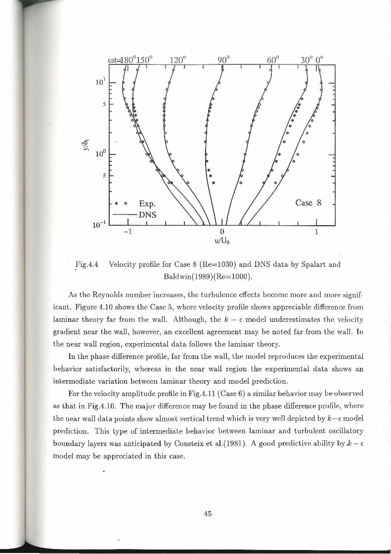
• 0
-1 0 u!Uo
Case 8
1
.Fig.4.4 Velocity profile for Case 8 (Re=l030) and DNS data by Spalart and
Baldwin(1989 )(Re= lOOO).
As the Reynolds number increases, the turbulence effects become more and more signif
icant. Figure 4.10 shows the Case 5, where velocity profile shows appreciable difference from
laminar theory far from the wall. Although, the k - t: model underestimates the velocity
gradient near the wall, however, an excellent agreement may be noted far from the wall. In
the near wall region, experimental data follows the laminar theory.
In the phase difference profile, far from the wall, the model reproduces the experimental
behavior satisfactorily, whereas in the near wall region the experimental data shows an
intermediate variation between laminar theory and model prediction.
For the velocity amplitude profile in Fig.4.11 (Case 6) a similar behavior may be observed
as that in Fig.4.10. The major difference may be found in the phase difference profile, where
the n.ear wall data points show almost vertical trend which is very well depicted by k - t: model
prediction. This type of intermediate behavior between laminar and turbulent oscillatory
boundary layers was anticipated by Cousteix et al.(1981 ). A good predictive ability by .k- t:
model may be appreciated in this case.
45

Fig.4.5 Fluctuating velocity in x-direction for Case 8 (Re= l030) and DNS data by
Spalart and Baldwin(1989) (Re=lOOO).
The development of turbulence characteristics may be noted from Fig.4.12. Here again,
the model predictions show quite good agreement with the experimental data. In Case 8,
where the Reynolds number is sufficiently high, the agreement of the k - E model prediction is
excellent in whole of the cross-stream dimension(Fig.4.13). The phase difference profile also
has been satisfactorily reproduced by the model except near the wall, where it overestimates
the phase difference.
An overall observation of all the figures presented herein reveals that although there exist
some discrepancies, the overall development of the transitional properties in case of mean
velocity amplitude and phase difference profiles in oscillatory boundary layer is efficiently
predicted by the original version of low Reynolds number k - E model(JL).
46

10°
5
,..-... e (.) '-" ;;....,
10-1
5
10°
5
,..-... e (.) '-" ;;....,
10-1
5
0
0
0
---laminar( theory)
-----k-E
10
0
20 u(cm/sec)
20 e(deg)
30 40
40
Fig.4.€> Mean velocity amplitude and phase difference profile for Case 1.
47

,-..._
s u
"---' >.
o Exp.(Case 2)
10° laminar(theory)
-----k-E 5
10-2 ~~~~~--~~~-L~--~~~-L~~~~~-L~~ 0 10
10°
5
10-1
5
0
20 u(cm/sec)
20 6(deg)
30 40
40
Fig.4.1 Mean velocity amplitude and phase difference profile for Case 2.
48

10°
5
,.-... s (.) '-" >.
10-1
5
10°
5
,.-... s (.) '-" >.
10-1
5
0
--laminar( theory)
-----k-E
20
0
fi(cm/sec)
20 8(deg)
0
40 60
40
Fig.4.8- Mean velocity amplitude and phase difference profile for Case 3.
49

10°
5
,....._ s (.)
"-" >.
10-1
5
0
--laminar( theory)
-----k-E
20
0
40 u(cm/sec)
20 6(deg)
60 80
40
Fig.4.9 -Mean velocity amplitude and phase difference profile for Case 4.
50

10°
5
,-.... s u '-" >-.
10-1
5
10°
5
,-.... s u '-" >-.
10-1
5
10-2
0
---laminar( theory)
-----k-E
20
0
o\
40 u(cm/sec)
lo lo I o I 0 I I I \ \ \
20 8(deg)
60 80
40
Fig.4.l0 Mean velocity amplitude and phase difference profile for Case 5.
51

"""' s C) '-' ;;...,
o Exp.(Case 6)
10° laminar(theory)
-----k-c: 5
10-2 ~--~~4-~--~----~----~--~----~--~----~~ 0
10°
5
10-1
5
10-2 0
20
'Q,_'Q_
'
40 u(cm/sec)
0"-0 ',
\
\
8 \ ol
~ I I I \ \ \
20 6(deg)
60 80
40
Fig.4.1i Mean velocity amplitude and phase difference profile for Case 6.
52

0
10° laminar( theory)
-----k-E 5
,--...
s u '-" >-.
10-1
/'7
5 ............
............ ............
............ ..................
............ /
// .. 10-2
//
0 20 40 60 80 u(cm/sec)
10° ''Q 5
"~ ,--... o',, 5 '-" 0 '\ >-.
10-1 \ 0 \ 0 I o I
5 oh I I I \ \
10-2 \
0 20 40 8(deg)
Fig.4.1'2 Mean velocity amplitude and phase difference profile for Case 7.
53
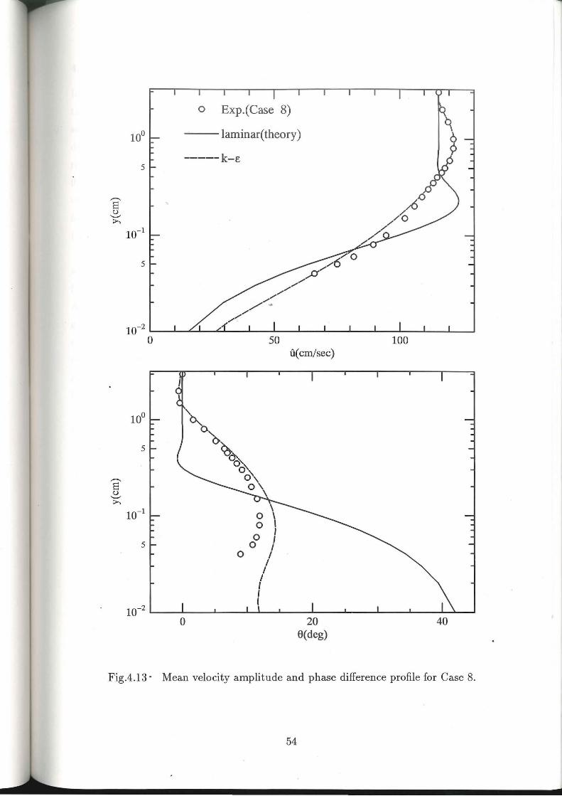
o Exp.(Case 8)
1 o0 laminar( theory)
-----k-E 5
50 100 u(cm/sec)
10° ' ~ 'o
5 ~ ~' o':-..
,.--._ o, s 0\ u \ '--' ;;.....
10-1 \ 0 \ 0 I
0 I I 5 0 I
0 I I I I I I
10-2 I
0 20 40 8(deg)
Fig.4.13 · Mean velocity amplitude and phase difference profile for Case 8.
54

4.5.2 Fluctuating velocity
In order to further elucidate the performance of the model during the phenomenon of transi
t ion in oscillatory boundary layer, the distribution of fluctuating velocity is presented in this
subsection. The contour plots of the fluctuating velocity in x direction from the experimental
data have been presented in order to appreciate t he changes occurring during t ransitional
regime. In Fig.4.14 and 4.15 although there exist some patches of appreciable turbulence
'fluctuations near t he wall, yet the ihtensity of t hese patches is low. T he beginning of a
visibly high fluctu a_ting velocity may be observed from Fig.4.16. It may be recalled that the
first signs of turbulence may be observed from mean velocity profile for this case also (see
Fig.4.8).
The turbulence patches lie exactly at the point of reversal of velocity(t/T ~ 0.25),
which shows that the presence of a negative portion near the wall and a positive one far
from the wall in velocity profile is responsible for the initial production of turbulent eddies . .
A similar shape of velocity profile exists in case of purely laminar flow also, but the velocity
gradient is not so steep to produce sufficiently strong eddies those may survive in viscous
environment. According to the regimes of flow as described by Hino et al.(1976) this flow
may be considered as weakly turbulent flow or Regime 2. A similar location of turbulence
generation has been shown by Hino et al.(1976) under this regime. Moreover , Jensen(1989)
has also reported similar turbulence properties at Re = 560.
A truly significant turbulence production near the beginning of deceleration phase and
its distribution in cross-stream direction during acceleration phase is evident from Fig.4.i 7.
A similar behavior has been reported by other researchers also see e.g. Jensen(1989). Most
of the turbulence is however, confined near the wall in this case. As the Reynolds number
increases, the production and distribution phenomena become more and more prominent in
a wave cycle. The region under influence of turbulence fluctuations in cross-stream direction
also increases as may be seen from Fig.4.18 to Fig.4.21.
4.5.3 Prediction of turbulence intensity
The model conforms to the laminar theory unto Re = 527, therefore the turbulence kinetic
energy in Case 1, 2 and 3 is negligibly small. Here the comparison will be made for the rest
of cases where the model shows appreciable amount of turbulence energy.
In order to make the comparison for x direction fluctuating velocity u' , an approximation
is used , since the model provides turbulent kinetic energy k, from which fluctuating velocity
in x-direction can be approximated as ,
u' = 1.052Vk ( 4.4)
a relationship derived from the experimental data for steady flow (see Nezu, 1977).
55

Case 1
u'(cm/sec)
2.5 0
0
0.00 0 .20 0.40 t / T
0.60 0 .80
Fig.4.14 Contour plot of fluctuating velocity for Case 1.
Case 2
u'(cm/ sec)
0 .00 0 .20 0 .40 t / T
0 .60 0 .80
·Fig.4.15 Contour plot of fluctuating velocity for Case 2.
56

Case 3
u'(cm/sec) 2.50
2.00
s C) 1.50 D
-.......--:>..
0 .20 0.40 t / T 0.60 0 .80
Fig.4.16 Contour plot of fluctuating velocity for Case 3.
Case 4 3.UUjj-----,-~~~--~~--------T-----~--~--~~~
u'(cm/sec)
0 .20 0.40 t / T
0 .60 0.80
· Fig.4.17 Contour plot of fluctuating velocity for Case 4.
57
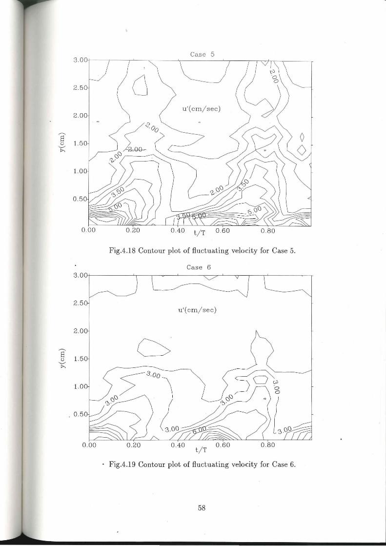
Case 5
2.50
u'(cm/ sec) 2. 00
s () 1. 50 .__.., ::>,
0 .20 0 .40 t/ T 0 .60 0 .80
Fig.4.18 Contour plot of fluctuating velocity for Case 5.
Case 6
2 .50 u'( cm / sec)
2 .00
s () 1.50
--.....,;
::>,
1.00
0 .50
0.00 0 .20 0 .40 t / T
0 .60 0 .80
· Fig.4.19 Contour plot of fluctuating velocity for Case 6.
58

Case 7
2 .50
2.00 u '(cm/sec)
8 0 1. 50
"-...-/
~
t / T 0 .80
Fig.4.20 Contour plot of fluctuating velocity for Case 7.
Case 8
u ' (cm / sec)
2.00
0.50
0 .20 0.40 0.60 0 .80
t / T
Fig.4.21 Contour plot of fluctuating velocity for Case 8.
59

The comparison made heretofore may thus be observed keeping in mind the fact that
this approximation may not be applicable in the whole range of cross-stream dimension as it
is based on the assumption of isotropic turbulence. In other words far from the wall, where
the flow is practically isotropic, this expression may yield better approximation as compared
to the region near the wall where the flow is essentially nonisotropic .
Figure 4.22 shows the comparison between model prediction and the experimental data
.for Case 4. The model can very well reproduce the cross-stream variation of u' far from the
wall. Although, near the wall some discrepancy may be observed, however, it is difficult to
attribute it to the -model alone because of the approximation used to compute u' . In the
deceleration phase(wt = 0- 37!"/8) the agreement is not so good, but during acceleration(wt = 1r /2 - 7n-j8), model shows an excellent predictive ability. The peak of fluctuating velocity
near the wall is underestimated by the model.
For Case 4(Fig.4.23), a similar tendency as in Case 4(Fig.4.22) may be observed. But
in this case, the agreement during deceleration is also satisfactory. For a higher Reynolds
number as compared to that in previous cases, the experimental data shows higher magnitude
of u' near the wall(Fig.4.24). The peak of u' profile during wt = n /8 - 1r /4 could not be
reproduced by the model. In all the other phases, the agreement with the data is good. In
Fig.4.25 also the disagreement between model prediction and the data is significant during
deceleration phase, but during acceleration phase, the model prediction is excellent.
Case 8 is the one with the highest Reynolds number in the present study. It may be
observed from Fig.4.26 that shape of the u' profiles predicted by the model during decelera
tion phase and a part of the acceleration phase(wt = 3n/ 4- 7n/8) are quite different near
the wall. The data depicts pointed peak of u', while the model shows a gradual variation in
cross-stream direction.
4.5.4 Boundary layer thickness
In the literature one may find three different definitions of oscillatory boundary layer thick
ness 8, i.e. after Jonsson (1963) who defines the boundary layer thickness to be the minimum
distance from the wall to a point where the velocity equals free stream velocity at wt = 0,
according to Jensen(1989) the distance from the wall to the point of maximum velocity
amplitude at wt = 0 and Sleath (1987) expresses the boundary layer thickness to be the
distance from the wall to a point where defect velocity amplitude is 5% of the free stream
velocity amplitude.
In case of laminar flow the boundary layer thickness can be found analytically according
to the three definitions from the expression for velocity profile. The definitions when applied
to the velocity profile yield the boundary layer thickness in terms of wave Reynolds number.
60

10° 5 Case 4
s 0 0 * 10-1
0 0 0 0 0
0 0 0
5 0 0 0
0 0 0 0
10-2
10° 5
,-..
§ ">: 10-1
5
10-2 0 5 10 0 5 10 0 5 10 0 5 10
u'(cm/sec) u'(cm/sec) u'(cm/sec) u'(cm/sec)
Fig.4.22 Prediction of u' for Case 4.
Case 5
10-2 ~~~~~~~~~~~~~~~~~~~~~~~~~~~~~~ 0 5 10 0 5 10 0 5 10 0 5 10
u~(cm/sec) u'(cm/sec) u'(cm/sec) u'(cm/sec)
Fig.4.23 Prediction of u' for Case 5.
61

10°
5 Case 6
§' 0 ·
~ 10-1 0
0
0 5 0 0
0 0
10-2
10°
5 ,.-....
§ 0
~ 10-1 00 0
0 0 5 0 0
0 0 ;,.
10-2 0 5 10 0 5 10 0 5 10 0 5 10
u'(cm/sec) u'(cm/sec) u'(cm/sec) u'(cm/sec)
Fig.4.24 Prediction of u' for Case 6.
10°
5 ,.-.... s u 0 0 ~ 10-1 0 0
0 0
5 0 0
0 0 0
10-2
10°
5 ~
§ 0
~ 10-1.
5 0 0
u'(cm/sec) u'(cm/sec) u'(cm/sec) u'(cm/sec)
Fig.4.25 Prediction of u' for Case 7.
62
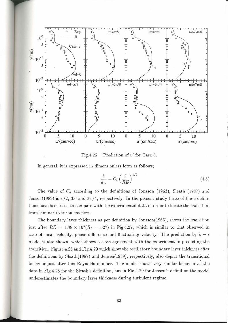
0 0 0
0 0
Case 8 ~0 »% 0 0 0 0
0 0
0 0 0 0 0
0
5 10 0 5 10 0 5 10 0 5 10 u'(cm/sec) u'(cm/sec) u'(cm/sec) u'(cm/sec)
Fig.4.26 Prediction of u' for Case 8.
In general , it is expressed in dimensionless form as follows;
8 - ( 2 ) 1/2 -- Cs -am RE
( 4.5)
The value of Cs according to the definitions of Jonsson (1963), Sleath (1987) and
Jensen(1989) is 1r /2, 3.0 and 31f /4, respectively. In the present study three of these defini
tions have been used to compare with the experimental data in order to locate the transition
from laminar to turbulent flow.
The boundary layer thickness as per definition by Jonsson(1963), shows the transition
just after RE = 1.38 x 10⁵ (Re = 527) in Fig.4.27, which is similar to that observed in
case of mean velocity, phase difference and fluctuating velocity. The prediction by k - E
model is also shown, which shows a close agreement with the experiment in predicting the
transition. Figure 4.28 and Fig.4 .29 which show the oscillatory boundary layer thickness after
the definitions by Sleath(1987) and Jensen(1989), respectively, also depict the transitional
behavior just after this Reynolds number. The model shows very similar behavior as the
data in Fig.4.28 for the Sleath's definition, but in Fig.4.29 for Jensen's definition the model
underestimates the boundary layer thickness during turbulent regime.
63

'2 0 Vl Vl !=: 0 ~
6
0.04
present Exp.
-- laminar( theory)
k-E
;% 0.02
+ + +
0~--~--_. __ _.~_.----~--~~~----._--~ __ ._ __ ~--~ 103 105 106 107
RE
Fig.4.27 Oscillatory boundary layer thickness as per definition by Jonsson(1963) .
0..1 .-----..------r----r----.-------,.-----..------.------.----.----r------.r------.
o present Exp.
---laminar( theory)
+ k-E
+ + + .
Fig.4.28 Qscillatory boundary layer thickness as per definition by Sleath(1987).
64

o present Exp.
---laminar( theory)
+ k-E
+ + +
Fig.4.29 Oscillatory boundary layer thickness as per definition by Jensen(1989) .
4.5.5 Friction factor and phase difference
In the present experiment the wall shear stress was not measured directly, therefore it was
computed from the velocity profile by momentum integral method. According to this method
the equation of motion for oscillatory boundary layers (Eq.3.4) is integrated from the wall to
the axis of symmetry of the tunnel. The wall shear stress computed by this method shows
large fluctuations. Jensen(1989) has described various reasons why these fluctuations occur.
In the present study, the first harmonic component of To was taken and its amplitude was
considered to be tauom· Using this value of maximum wall shear stress the friction factor
was computed employing Eq.(3.13). Figure 4.30 shows the friction factor diagram showing
the present data. The experimental data by Jensen(1989) is also shown. It may be observed
that there is a close agreement between both the experimental data. The present data
for Case 1 and 2 lies within laminar regime and it may be observed that both these data
points follow the lamintheory. The transitional effects start just after RE = 1.38 x 10⁵ (Case
3) in accordance with the findings in previous sections. The prediction by low Reynolds
number k - E model have also been shown and it is found that the model can predict the
transitional behavior in an excellent manner. Moreover, the predictions during laminar and
fully turbulent regimes also the model prediction is good.
65
' -

The phase difference ()0 between the max1mum wall shear stress and the maximum
velocity at the axis of symmetry was found by extrapolating the phase difference profiles
to the wall. The value of ()0 thus obtained is plotted in Fig.4.31. Here also the present
experimental data shows quite good agreement with the experimental data by Jensen(1989).
The starting point of transition is just at RE = 1.38 x 10⁵ (Case 3). As may be observed
that during the transition phase difference value falls rapidly until after RE ~ 3 x 10⁵ it
decreases gradually with the increase in Reynolds number . It merely shows that during
transition the momentum t ransfer from high velocity regions to t he low velocity regions is
very high and this effect then increases the homogeneity of the flow in cross stream direction .
The prediction by k - t: model in this case also reproduces the variation of phase difference
with Reynolds number satisfactorily. 10-1 ~--~---T---T--~----~--~--~----~--~--~--------
0 present Exp.
5 laminar( theory)
+ k-E
D. Exp.(Jensen,1989)
J 10-2
5 ~+~+ D.+ D.~
10-3 ~--L---~--~~~----~--~~~----~--~--~--~--~ 103 105 106 107
RE
Fig.4.30 Friction factor for oscillatory boundary layer.
66
' .. l ...

l::.
0
laminar( theory)
0 Ex~ ~ +
present study ~++~ k-E
l::. Exp.(Jensen,1989) 0 l::.+ + l::.
l::. 0 Exp.(Sawamoto & Sa to, 1991)
0~--~---L---L~-L----~--~--~----L---~--L---~--~ 103 104 105 106 107
RE
Fig.4 .31 Phase difference for oscillatory boundary layer.
4.6 Conclusion
As a result of the present study to check the applicability of low Reynolds number k - t:
model to the transition from laminar to turbulence in an oscillatory boundary layer, the
following conclusions may be drawn;
1. The model can very well predict the velocity and phase difference during transition.
2. The fluctuating velocity in x direction is predicted in an excellent manner during
acceleration phase, whereas some discrepancies were found during deceleration phase
near the wall. The final conclusion in this case however is difficult due to the use of
an approximation to calculate u' from k value.
3. The change in boundary layer thickness as per definitions by Jonsson and Sleath during
the transition was reproduced by the model efficiently, but for Jensen's definition, the
model underestimates the boundary layer thickness in turbulent regime.
4. The fricti~n factor and phase difference during transition is predicted in a good manner
by the low Reynolds number k - t: model.
67

5 PERFORMANCE OF k - E MODEL TO
ANALYZE THE BOUNDARY LAYERS UNDER
WAVE-CURRENT COMBINED MOTION
5.1 General
In coastal environments the combined effects of waves and current have a major influence
on the sediment movement . The number of st udies on t his topic is thus very large. As '"
mentioned in Chapter 2, major contribution to this effect is by semi-empirical and analytical
approaches . The abundance of present day computational resources have encouraged the
coastal engineers to move on to more rigorous modeling approaches. Although some of the
researchers have tried to use higher order turbulence models , however, k- E is an appropriate
choice to analyze various engineering flows due to its reasonable accuracy with computational
economy.
In Chapter 3 some of the modern versions along with the original one were applied to an
oscillatory boundary layer. The original model( JL) was found to be promising by virtue of
its ability to predict" the transitional characteristics and two of the latest versions; MK and
NT reproduced the turbulence magnitude in an excellent manner. Therefore, these three
models have been selected to analyze the boundary layer under the combined effect of waves
and current in the present study.
The governing equations of these models have already been given in Chapter 3. Only the
equation of motion Eq.(3.21) needs to be modified to include the effect of current magnitude.
The modified equation of motion in dimension-less form may be given as;
ou* (~ * ~ * ) s a { ( s *) ou*} ot* = Ps + Pw + oy* RE + vt oy* (5.1)
With all the variables defined already, steady component of the pressure gradient is expressed
by ~p:.
In order to produce the average current magnitude < u > equal to that in the experi
ment, initially an arbitrary value of ~p: was imposed, which was then refined to achieve the
experimental value of current magnitude.
5.2 Experimental Data
This experiment was performed in a U-shaped oscillating tunnel equipped with a centrifugal
pump to generate the uniform flow as described in Chapter 4. With this equipment , it is
easy to control the current magnitude independently. The velocity was measured using one
component LDV in forward scatter mode, the experimental setup being given in Chapter
68

4. The wall shear stress was computed by assuming the logarithmic velocity profile in the
near-wall region. The experimental conditions for COl and B05 are presented in Table
5.1, where,< u >is the cross-stream averaged current magnitude and Rc(= < u >yh/v) is
current Reynolds number.
Table 5.1. Experimental conditions for the boundary layer under wave-current combined
motion.
Exp. Yh( cm) T(sec) < u >(em/sec) Uo( em/sec) Rc RE
COl 3.00 - 8.4 - 2217 -
B05 3.00 2.84 8.9 116.8 2345 5.4 X 10⁵
It should be noted that in Case B05 the oscillatory component is the same as in Case
8 presented in Chapter 4. The superimposed current magnitude is 7 percent of the total
velocity amplitude at the axis of symmetry. Thus Case B05 represents the case of a pulsatile
motion in wave dominant environment.
5 .3 Interaction of Mean and Oscillatory Components
5.3.1 Effect of the current on oscillatory boundary layer
A nurriber of experimental studies by other researchers have proved that in a wave dominant
environment, the effect of current on the wave boundary layer is negligible. Figure 5.1,
showing the oscillatory velocity amplitude and phase difference profiles for Case 8 and B05,
supports this fact. A close observation of the figure however, reveals that in the present case
of boundary layer under wave-current combined motion, the velocity profile near the wall
is a little steeper as compared to that in pure wave boundary layer. The phase difference
profile is just the same for both the cases.
5.3.2 Deformation of the current profile by oscillatory boundary layer
The thickness of oscillatory boundary layer is very small as compared to that of steady one.
That is why the velocity gradient near the wall, in case of oscillatory boundary layer, is
very steep. Therefore, the current velocity profile near the wall is mainly affected by the
oscillatory motion. It may be observed in Fig.5.2 that for Case B05 the current velocity
gradient near the wall is steeper than the pure current case COl. This is in agreement with
the findings of Kemp and Simons(1982) as a result of their experiment under waves 'with
following current on a smooth bottom. In their study they have shown that for a rough
bottom, the velocity gradient becomes milder as compared to the current alone near the
wall. In the present case this deformation in the current profile occurs at y = 8, where 8
69

is the boundary layer thickness as per Jonsson's definition. Above this level also, the mean
current profile under combined motion steeper than the one in current alone case COL It
may be attributed to the increased amount of momentum transport towards the wall and
free-stream from the region of high velocity.
5.3.3 Increase in turbulence intensity
·As mentioned before the major changes in the mean properties occur within the region from
wall to oscillatory boundary layer t hickness , but in case of fluct uating velocity, the interaction
between mean and oscillatory components prevail over the whole cross-section of the flow .
It is obvious that due to the action of steep velocity gradient of oscillatory component near
the wall, more turbulence energy is produced. This energy is then distributed in the cross
stream direction. That is why, the fluctuating velocity magnitude at the axis of symmetry
in pulsatile motion does not attain the corresponding value in pure current case as shown in
Fig.5 .3.
5.4 Model Predictions
From Fig.5.4, 5.5 and 5.6 , it is clear that the prediction of velocity by the three models is not
so diffe.rent . Though, all of them underestimate the velocity gradient in the near wall region ,
however, the overall predictive ability is satisfactory, in this regard. Especially the velocity
over-shooting is predicted very well, and the agreement far from the wall is excellent. The
prediction by JL model is slightly better than the other two models in this case.
Probably, the major discrepancy, revealed here, is in the prediction of period averaged
mean velocity profile as depicted by Fig .5. 7 (the period averaged quantity is expressed by
<> ), where, the near wall behavior could not be simulated by any of the models under
consideration. It is a well established fact that in the near wall region of a wave-dominant
flow, the current velocity profile is distorted by the action of wave boundary layer. This
behavior is very well depicted by the experimental data, but this complex phenomenon
could not be reproduced by any of the models. In order to make comparison with the
experimental data in the present study, again the approximation is used to compute u' from
k, i.e. Eq.(4.4).
in Fig.5.8 , the profiles of u' for selected instant are plotted. Although, all the models
seem to be unable to predict the variation of u', in the deceleration phase (tjT = 0.12, ~.24),
near the wall , however , in acceleration phase (t/T = 0.36, 0.48), good agreement is found. A
similar behavior was observed in case of oscillatory motion also , as shown in Chapter 3 and
4.
All the models underpredict u' far from the wall, but showing good agreement near the
70

free-stream. The JL model underestimates u' near the wall at almost every instant during the
course of a wave cycle. It may be noted that this comparison depends on the approximation
also(Eq.(4.4)), which was used here.
Figure 5.9 depicts that MK and NT models are supenor to JL model in predicting
< u' >. Although the agreement far from the wall is not satisfactory by any of the three
models , however, very near the wall and at the axis of symmetry good agreement has been
shown by MK and NT models.
Figure 5.10 shows that the wall shear stress prediction by MK and NT is much more
close to the experimental value in magnitude, as compared to that by JL model. The reason
for the underestimation by JL model is in fact due to the underestimation of turbulence
fluctuations as shown in Fig.5.8 and Fig.5.9, which in turn leads to low eddy viscosity
and consequently less magnitude of wall shear stress. As may be noted from Fig.5.10 that
although, there exists a. discrepancy in predicting the phase difference, however, all the three
models can show nonlinear variation over the wave cycle to some extent.
The experimental data shows stepping of the wall shear within phases of about 45° and
135° and then from 270° to 310°. Three of the models show, though very mild, a similar
behavior in these ranges.
71

---<r- Exp.(Case 8)
10° ---+--- Exp.(B05)
5
u(cm/sec)
10°
5
,-..._
s (.) "-' ;;;....
10-1
·5
0 10 8(deg)
Fig.5.1 · Velocity amplitude and phase difference profile for Case 8 and B05.
72

10°
5
--. § '-" :>-.
10-1
0
. 3
2
1
0
-o-Exp.(COl)
---+--- Exp.(BOS)
b(Jonsson)
5 <u>(cm/sec)
Fig.5.2 Current profile Case COl and B05.
t I I I I I I I I I I I
+. \ \
\ \
\ \
-\ \
\ \
\ \
' ~ ' ' +..
'
-o-Exp.(COl)
---+--- Exp.(BOS)
'+.. +--±
"I".>L
'* ...... _+--+--+-
5 <u' >(cm/sec)
Fig.5.3 Period average fluctuating velocity.
73
10
10

10°
5
,-.,. s u '-" :>-.
10-1
5
10°
5
,-.,. s u '-" :>-.
10-1
5
t!T= .54 .48 .42 .36
-100
.3
0 u(cm/sec)
.24 .18 .12
100
Fig.5.4 Predicted velocity profile for case B05 by JL model.
.54 .48 .42 .36
-100
.3
0 u(cm/sec)
.24 .18 .12 .06
100
Fig.5.5 Predicted velocity profile for case B05 by MK model.
74

10°
5
,-... s u '-" ;:;.-,
10-1
5
.54 .48 .42 .36
-100
.3
0 u(cm/sec)
.24 .18 .12
100
Fig.5.6 Predicted velocity profile for case B05 by NT model.
..•. .•. .....
0
Fig.5.7
.•. .•.
5 <u>(cm/sec)
··· ·· ·• ·····Exp .
-------JL
-----MK
- ·-NT
Period averaged velocity for case B05.
75
10

5
5
5
0
5
0
\ •",
•\\ ·i~ ·~~ ':~-:~ . ·',~~ . '~~ . \
. --~, • Exp. • \
-------JL -----MK -·-NT
I ,
5 10 u'(cm/sec)
0 5 10 0 u'(cm/sec)
Fig.5.8 Profiles of fluctuating velocity.
76
\ • t/T=0.18
• I '-4~. .-~~ . ',,.
5
. '~~ '~
• $ \\· • I • I
I
·. i\ •' I • •
10 u'(cm/sec)

•
0
Exp .
JL
MK
NT
5 <u'>(crn/sec)
Fig.5.9 Period averaged fluctuating velocity.
50 Exp.
-------JL
-----MK
-·-NT
0
10
-50~~~-~~~--~~~--~~~--~~~--~-L~~
360 0 60 120 180 mt(deg)
240
Fig.5.10 Wall shear stress for case B05.
77
300

5.5 Conclusion
The major conclusions obtained from the study presented in this chapter are ;
1. In a wave dominant pulsatile motion, the oscillatory component of the boundary layer
is nearly unaffected by the current.
2. In this type of motion however, the current profile is deformed, and the effect of this
deformation is prominent unto a distance equal to oscillatory boundary layer thickness
as per defini tion by Jonsson.
3. The period averaged turbulence intensity is enhanced by the action of oscillatory
boundary layer and its effect prevails over the whole cross-stream dimension.
4. The three models under consideration, i.e. JL, MK and NT, perform well in predicting
the velocity profile. However , MK and NT models are superior by virtue of their better
performance regarding the fluctuating velocity and the wall shear stress.
5. The pulsatile boundary layer may be regarded as an excellent test case for the testing
of turbulence models.
78

6 ASYMMETRIC OSCILLATORY BOUNDARY
LAYERS
6.1 General
The oscillatory boundary layers under natural coastal environments are generally different
. from purely sinusoidal ones. There have been numerous efforts to predict the actual wave
profiles in the field . Cnoidal wave theory is one of the important theories in order to reproduce
the water surface profile in coastal environments. The cnoidal waves belong to the permanent
wave category in the vicinity of Ursell parameter equal to unity. The name cnoidal is given
due to the fact that the wave profile is expressed in terms of en function of Jacobi's elliptic
functions, and using the analogy of sinusoidal wave, the word cnoidal is derived.
Although this type of asymmetric wave boundary layers are important as their pres
ence is a commonplace in the real field situations, however, studies regarding them are very
few. Especially experimental studies are almost nonexistent due to the reason that it is very
difficult to produce such type of wave profile in the laboratory but with highly expensive com
puter controlled wave generation system. Asano and lwagaki(1986) discussed the boundary
layer properties under asymmetric waves numerically. They performed a few experiments
also to·check the validity of their solution on a rough bottom. Nadaoka et al.( l994) carried
out a detailed experiment probably for the first time by using recirculating tunnel equipped
with a sophisticated piston controlled mechanism. They reproduced hyperbolic wave profile
at the axis of symmetry, which is very similar to the cnoidal wave. They used air as the
working fluid and wall condition was smooth. The Reynolds number in that study was not
high enough to produce fully developed turbulence. Ribberink and Al-Salem(1995) carried
out the experiments in an oscillating water tunnel , but their interest was in the sheet flow
and sediment suspension in case of asymmetric waves. Larsen(1995) used a time-invariant
eddy viscosity model to predict the velocity profile under asymmetric waves. The predictions
were compared with the experimental data by Nadaoka et al.(1994), but the pronounced ve
locity overshooting could not be reproduced by the model. Nadaoka et al.(1996) performed
the experiments by using the same experimental facility as was employed by N adaoka et
al.(1994) and measured the velocity by two component LDV under asymmetric oscillatory
motion. They showed that the reason for more turbulence energy production in asymmetric
case than the corresponding sinusoidal case is the higher velocity gradients during t:cough
phase in the former case.
In the pre~ent study a novel piston movement system was developed. The system does
not require sophisticated electronic devices to generate the asymmetric oscillatory motion,
thus inexpensive to install and use. Initially air was used as the working fluid , but due to
79

the constraints involved in the oscillating tunnel, it was impossible to generate turbulent
flow. Therefore, water was used as the working fluid in order to generate turbulent flow.
The velocity profiles were measured in detail to observe typical behavior of the boundary
layer under cnoidal waves.
The numerical prediction was made by using the low Reynolds number k- f. model( JL).
As described before, this model has been very efficient in predicting the transitional proper
, ties of sinusoidal oscillatory boundary layers.
6.2 Experimental System
The experiments were performed in aU-shaped oscillating tunnel with smooth walls similar
to the one described in Chapter 4. Here the cross-section of the measurement section was
17cm(width) x6.5cm( depth) and the length of straight part of the tunnel was 180cm. The
velocity measurement equipment is same, i.e. fiber optic LDV as described in Chapter 4.
6.2.1 Piston movement system
The basic idea of this system is based on the variation of linear velocity along the circumfer
ence of a circular disc rotating with constant angular speed. In the present system a circular
disc is .rotated by an electric motor. At a certain distance a from the axis of the disc a
bearing is placed(Fig.6.1). This bearing can oscillate in a slot made along the length of a
flat metallic plate, which is hinged at its lower end.
b
,--.x <I>
I I
I .I
_ _j ___ _
~ a
l
Fig.6.1 Piston movement system to generate cnoidal wave motion.
At a vertic~l distance l above the hinge, another flat plate is held horizontally. Both the
ends of this horizontal plate are attached to the two pistons. The cylinders containing the
80
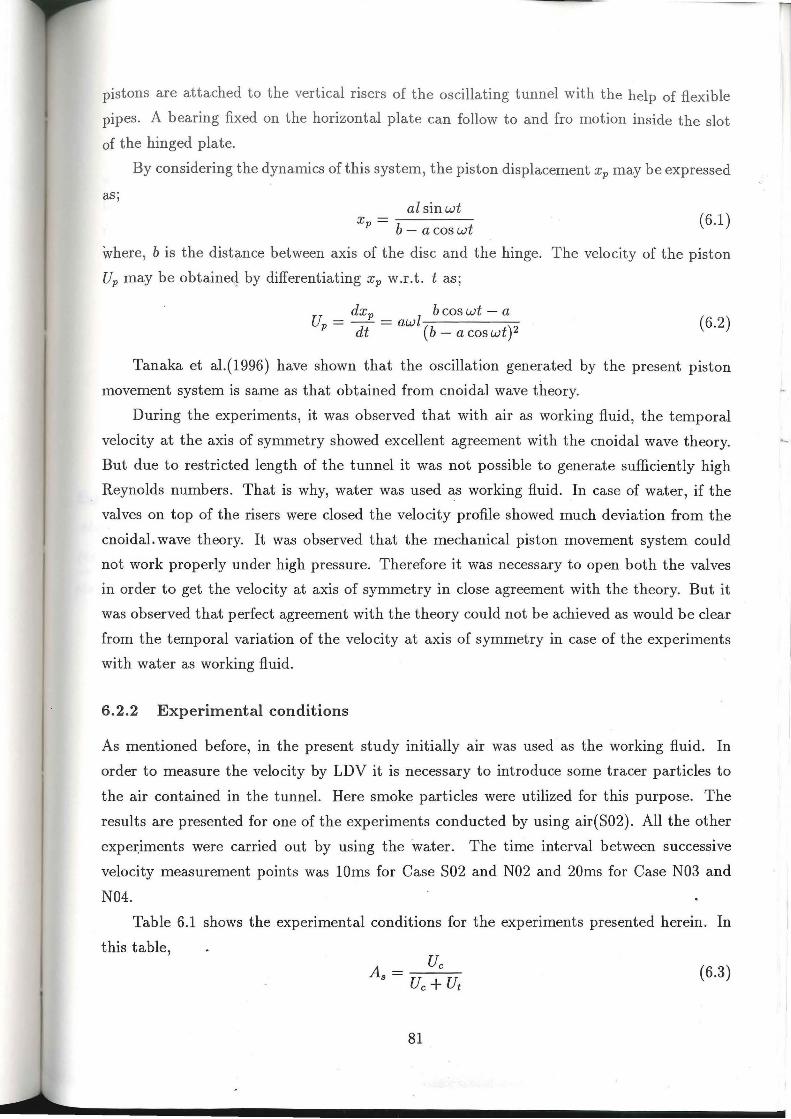
pistons are attached to the vertical risers of the oscillating tunnel with the help of flexible
pipes. A bearing fixed on the horizontal plate can follow to and fro motion inside the slot
of the hinged plate.
By considering the dynamics of this system, the piston displacement xp may be expressed
as ; al sinwt
X = (6 1) P b- a coswt ·
where, b is the distance between axis of the disc and the hinge. The velocity of the piston
Up may be obtaineq by differentiating Xp w.r.t. t as ;
U = dxP =awl bcoswt- a P dt (b - acoswt) 2 (6.2)
Tanaka et al.(1996) have shown that the oscillation generated by the present piston
movement system is same as that obtained from cnoidal wave theory.
During the experiments, it was observed that with air as working fluid, the temporal
velocity at the axis of symmetry showed excellent agreement with the cnoidal wave theory. "-·
But due to restricted length of the tunnel it was not possible to generate sufficiently high
Reynolds numbers. That is why, water was used as working fluid. In case of water, if the
valves on top of the risers were closed the velocity profile showed much deviation from the
cnoidal. wave theory. It was observed that the mechanical piston movement system could
not work properly under high pressure. Therefore it was necessary to open both the valves
in order to get the velocity at axis of symmetry in close agreement with the theory. But it
was observed that perfect agreement with the theory could not be achieved as would be clear
from the temporal variation of the velocity at axis of symmetry in case of the experiments
with water as working fluid.
6.2.2 Experimental conditions
As mentioned before, in the present study initially air was used · as the working fluid. In
order to measure the velocity by LDV it is necessary to introduce some tracer particles to
the air contained in the tunnel. Here smoke particles were utilized for this purpose. The
results are presented for one of the experiments conducted by using air(S02). All the other
exper.iments were carried out by using the water. The time interval between successive
velocity measurement points was 10ms for Case 802 and N02 and 20ms for Case N03 and
N04.
Table 6.1 shows the experimental conditions for the experiments presented herein. In
this table,
(6.3)
81

(6.4)
(6.5)
where, Uc and Ut are velocity magnitude at crest and trough, respectively. The Stoke's
layer thicknesses for crest and trough are given as 81c (= J2vtcf';r) and 8~t(= J2vtt/7r),
respectively. The crest and trough periods are denoted by tc and tt , respectively. The
definitions of Rec and Ret have been adopted from Nadaoka et al.(1994). All the relevant
quantities are shown_ in the definition sketch (Fig. 6.2). ~~ ~ 1 ,'\_~ c-_ I
Table 6.1. Experimental conditions for asymmetric oscillatory boundary layer experiments
Exp. T(sec) tc(sec) tt(sec) Uc (cmjs) Ut(cm f s) v(cm2 / s) As Rec Ret ~
S02 2.15 0.83 1.32 161.3 88.0 0.1489 0.64 304 209
N02 2.00 0.84 1.16 109.4 66.9 0.0087 0.62 859 616 4
N03 2.38 0.98 1.40 89.3 56.0 0.0089 0.61 744 559 3 N04 3.92 1.66 2.26 55.6 42.7 0.0089 0.57 604 541 "Z
• \o~~
T
Fig.6.2 Definition sketch for the free-stream velocity under cnoidal wave.
82

6.2.3 Computation of wall shear stress
In the present study, the wall shear stress was not measured directly, therefore it was nec
essary to use the indirect methods to compute it from the velocity data. The most popular
computational methods are based on; (i) linear velocity variation in the viscous sublayer,
(ii) logarithmic profile in the overlap layer, and (iii) t he equation of motion.
In order to compute the wall shear stress To from first method, it is assumed that the
theory relevant to steady flow is applicable, whence within the viscous sublayer ,
or
u
u To = pv-
y
(6.6)
(6.7)
According to second method again following the steady flow theory, the logarithmic velocity
variation is assumed in the overlap layer where,
~ = ~ln (YUJ) + C Uj K 1/
(6.8)
where K is von Karman constant(=0.4) and Cis a constant. By plotting u against ln(y),
a straight line is drawn through the experimental data in overlap layer and To can then be
found from the slope of this line.
The third method is a general method according to which the equation of motion is
integrated from the wall to free-surface( axis of symmetry of the tunnel in the present case)
to obtain the wall shear stress, that is why this method is generally called as momentum
integral method.
All the above methods have their limitations due to the validity range of the respective
governing equations. In the first method, it is necessary to measure the velocity sufficiently
close to the wall, so that the point of measurement may lie within viscous sublayer. For low
Reynolds numbers it is possible, but as the Reynolds number gets higher, the thickness of
viscous sublayer decreases, so that the limitations involved in the measurement system do not
permit to measure the velocity within viscous sublayer. The second method is essentially
for quite high Reynolds number flows. Since at low Reynolds numbers the thickness of
logarithmic layer is very small. That is why, this method can not be successfully applied
to the cases within transitional region. For fully turbulent flows also this method is not
applicable within the period of oscillation near the velocity reversal. The third method is
sensitive to the small fluctuations in cross-stream velocity profile which gives rise to very
high fluctuations in the wall she;;t.r stress. It is thus required to carry-out smoothing of this
data in order to observe the variation of To clearly. Jensen(1989) has also reported difficulties
in applying this method to sinusoidal oscillatory boundary layers.
83

In all the present experiments the measurement point nearest to the wall was at a
distance of 0.02cm from it. In order to ascertain whether this point lies within the viscous
sublayer, so that Eq.(6.6) may hold, the thickness of viscous sublayer 8v was computed by
the following expression; 8 - 5.01/ v- FJP (6.9)
. where the wall shear stress To used in this expression was obtained from Eq.(6.7) as a first
approximation. The value of 8v obtained in such a manner is plotted in Fig.6.3. It may
be observed from this figure that the approximate viscous sublayer thickness is less than
the first measurement point near the wall during crest and trough periods for the cases
N04, N03 and N02, which shows that for these cases this method is not fully reliable. Case
S02 is in laminar regime as suggests the value of its Reynolds number (Rec = 304 < 550,
Ret = 209 < 550), therefore the first method may be applied.
Q.04
0~--~----~----~--_.----~----~--~----~----~--~ 0 0.5
ttr
Fig.6.3 The thickness of viscous sublayer in the present experiments.
1
In the present set of experiments the cases N04 and N03 lie within the transitional
regime as may be observed from the respective values of Reynolds numbers, therefore the
thickness of logarithmic layer is very small as would be clear from the velocity profiles for
these cases. In case N02 however, the logarithmic layer is prominent, thus it was possible
to compute To by logarithmic method. The third method, i.e. momentum integral method
is applicable to all the cases, therefore it may be used to compute the wall shear stress
84

invariably for all the cases.
6.3 Effect of Asymmetry in Cnoidal Wave
The relative difference between the crest and trough velocities is expressed by the degree
of asymmetry As. It may be observed from the definition of As that its value lies between
0.5 and 1.0. Figure 6.4 shows the free-stream velocity for selected values of the degree of
asymmetry as computed from Eq.(6.2). In a manner similar to that shown by Tanaka et
al.(1996) , the theoretical solution for cnoidal wave is also presented. According to the cnoidal
wave theory, the free-stream velocity U may be expressed as;
(6 .10)
where, en is the Jacobi's elliptic function and I< is the complete elliptic integral of the first
kind.
It may be observed that the present system can generate an asymmetric oscillation
similar to the cnoidal wave motion in an excellent manner. The important thing that may
be noted from this figure is that as the value of As increases, so does the sharpness of
crest and flatness of trough portion. On one hand, during the flow reversal, a more rapid
change .occurs as compared to an equivalent sinusoidal case and on the other hand, flatness
of velocity during trough phase causes the flow to develop in a way similar to that of steady
flow.
6.4 Laminar Flow
In case of a boundary layer under asymmetric waves , it is convenient to use Fourier com
ponents of the free-stream velocity in order to express the mean velocity in space and time
as;
m
u = L [an{sin nwt - exp( - yl 8zn) sin(nwt- yl 8zn)} n=l
+bn {cos nwt - exp( - y I 8zn) cos( nwt - y I 8zn)}) (6.11)
when~ an and bn are nth sine and cosine components of velocity at the axis of symmetry,
respectively and 81n ( = j 2v I nw) is the Stokes' layer thickness for nth component. By using
the Newton's law of viscosity and the above mentioned velocity, the wall shear stress.may
be expressed as;
m
To = p L vfnWi/{ an sin( nwt + 11" I 4) + bn cos( nwt + 11" I 4)} (6.12) n=l
85

The experiment on laminar boundary layer under asymmetric oscillation is considered
here to be important in order to get an insight of the nature of this type of boundary layer
as well as the validation of the present experimental setup.
Figure6.5 shows the temporal variation of velocity at the axis of symmetry along with
the piston displacement. The velocity profile at selected time intervals during the course of a
cycle is shown in Fig.6.6 . The theoretical solution from Eq.(6.10) is also plotted. The velocity
Qvershooting at the instant of maximum and minimum free-stream velocity seem to be similar
to the purely sinusoidal wave boundary layers qualitatively. An important property that is
evident from this figure is the difference of oscillatory boundary layer thickness under crest
and trough.
By using Jensen's definition, according to which the boundary layer thickness 8 is the
distance from the wall to the location of maximum cross-stream velocity at wt = 0 (or at
wt = T /2), it may be shown that the boundary layer thickness 8 is proportional to the
Stoke's layer thickness(= jvTj1r) , which suggests that the value of 8 must be greater under
trough than that under the crest due to longer period of time contained in the trough. The
result may be observed at tjT = 0.5 where the boundary layer thickness is greater than that
at tjT = 0. Another important point is the steep deceleration during crest phase(Fig.6.5).
In case of sinusoidal oscillatory boundary layers the turbulence spots are generated at this
point which corresponds to maximum value of aU I at and the flow becomes weakly turbulent
flow according to the classification by Hino et al.(1976). It may be anticipated that this type
of turbulence may be triggered earlier than in an equivalent purely sinusoidal case due to
steeper deceleration as compared to an equivalent sinusoidal case.
Figure 6.7 shows the wall shear stress from the experiment and the laminar theory for
Case S02. As may be recalled, in case of purely sinusoidal wave boundary layer in laminar
flow regime, shape of the wall shear stress is also sinusoidal, but there exists a phase difference
of 45° between free-stream velocity and r 0 • It may be noted from Eq.(6.11) that following
the same basic principle, every component of the wall shear stress has a phase lead of 45°
from the corresponding velocity component. But after the addition of these components with
each component having different number of waves in one cycle, the shape of the resultant
wall shear stress profile is altogether different from the corresponding free-stream velocity
profile over the wave cycle.
86
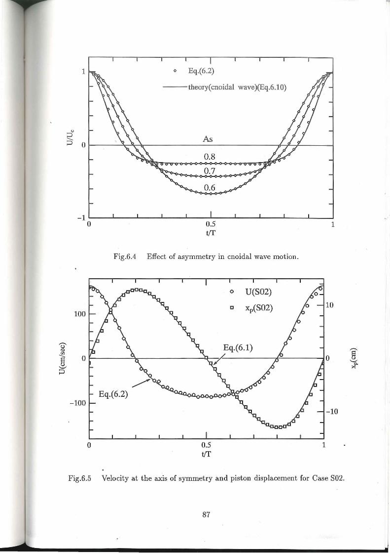
1 o Eq.(6.2)
---theory(cnoidal wave)(Eq.6.10)
u
~ Or-----~~~-----------A_s ____________ ~~r-----~
100
0.5 t{f
Fig.6.4 Effect of asymmetry in cnoidal wave motion.
o U(S02)
IJ Xp(S02)
Eq.(6.1) 0~----~~--------~~--------~----~
-100
0
~ Eq.(6.2)
0.5 tiT
1
1
10
-10
Fig.6.5 Velocity at the axis of symmetry and piston displacement for Case 802.
87

....-.-§
"-" >-.
t/T=0.4 0.3 0.2
5
0.1 0.0
• o Exp.(S02)
--laminar( theory)
10-2 ~~~~--~--~~~L-~--~--~--~--L-~~~--~~~ -100 0 100
u(cm/sec)
10°
5
10-1
5
u(cm/sec)
Fig.6.6 Velocity profile for Case S02.
88

The definition of phase difference in case of asymmetric oscillatory boundary layers is
not as simple as in sinusoidal case. Tanaka, Sumer and Freds¢e(1996) used separate values
for crest and trough, i.e. the phase difference in crest Oc is the phase lead of crest of wall
shear stress from crest velocity at the axis of symmetry, and similarly the phase difference
in trough may be defined by the corresponding trough values. The definitions of (}c and (}t
are shown in Fig. 6. 7. as may be observed that unlike the sinusoidal case, the value of (} c is
·less than Ot in the present asymmetric oscillatory boundary layer.
6.5 Turbulent Flow
As to the present day, the critical Reynolds number in case of asymmetric oscillatory bound
ary layers has not been studied in detail. As a first approximation however, the value for
purely sinusoidal oscillatory boundary layers may be considered to be applicable. But it
may be noted that in asymmetric case, although Reynolds number is of primary importance
like in sinusoidal case, it is not the only governing parameter. The difference of crest and
trough velocities or in other words, degree of asymmetry expressed by As also helps trigger
ing the turbulence production. With higher As value, the deceleration becomes steeper and
a lower value of Reynolds number may produce significant amount of turbulence than the
corresp.onding value for purely sinusoidal case.
6.5.1 Velocity profile
For Case N04 it may be noted that the Reynolds number in this case (Rec = 604, Ret= 541)
is in the range of transitional Reynolds number for sinusoidal oscillatory boundary layers as
given by previous researchers (see Hino et al.(l976)). Figure 6.8 shows the temporal variation
of velocity at the axis of symmetry U and the cross-stream velocity profile at selected phases.
As mentioned before, there is a slight difference between the velocity obtained at the axis of
symmetry and the cnoidal wave theory.
The velocity profile for Case N04 shows a better agreement with the k- t: model predic
tion just at the beginning of deceleration phase(t/T 0.0) as compared to the laminar theory,
especially where the velocity overshooting occurs. But during the course of deceleration, it
seems that the model fails to cope with the flow situations. The reason for that is unclear,
however, it may be attributed to the inability of this kind of model to reproduce the actual
length scale near the wall under adverse pressure gradient(APG) as has been shown by Rodi
and Scheuerer{l986) . It is still to be resolved which parameter of the model is to be modified.
89

100
-100
0
0 Exp.(S02)
--laminar( theory)
at axis of symmetry)
0.5 t/T
Fig.6.7 Wall shear stress for Case 802.
0
100
-100
1
One of the proposals is by Hanjalic and Launder(1980), that is to add another production
term in the transport equation of t to increase the dissipation rate under APG thereby
reducing the length scale since the length scale is inversely proportional to t. However, this
model is still controversial due to a rather larger value of the empirical coefficient used in
the additional term compared to that in the existing production term.
In the present case during deceleration the model shows logarithmic behavior at t j T =
0.1 and 0.2, whereas the data shows better agreement with the laminar solution near the
wall. It might be noted that in case of sinusoidal oscillatory boundary layers, during the
deceleration phase, pressure gradient is not so steep as in the present asymmetric case. That
is why, in the former case the disagreement with the experimental data is not pronounced
(see the previous Chapters).
As the flow proceeds to acceleration in the trough phase, the model predictions begin
to conform to the data very well. There remains, though, a discrepancy near the wall. In
the next deceleration during the trough phase(t/ T = 0.5 - 0.7), the model prediction is sat
isfactory because the pressure gradient is not so steep, but fine details of the velocity profile
could not be reproduced by the model. During the next acceleration phase(t/ T = 0.8 - 0.9)
an excellent agreement is found between prediction of the model and the experimental data.
The degree of asymmetry in Case N04 is not so high as may be observed from the value of
90

As(= 0.57) in this case. That is why the difference between boundary layer thickness under
crest and trough is not so significant.
For higher Reynolds number as in case N03 a considerably high degree of turbulence
may be expected in Case N03. From Fig.6.9 it may be inferred that in this case again the
agreement between model prediction and the experiment is poor during deceleration phase
but during acceleration the model could imitate the velocity profiles shown by the data, yet
with a discrepancy near the wall. This trend is similar to that depicted in Case N04(Fig.6.8) .
Unlike the previous case (N04), here the difference in boundary layer thickness under crest
and trough is visible due to the fact that the degree of asymmetry in this case is relatively
high (As= 0.61).
The case of highest Reynolds number presented herein is Case N02. The inability of
the model to predict the velocity profile in deceleration phase and good agreement during
acceleration phase is evident in this case also(Fig.6.10). Moreover, it may be observed that
the discrepancy between the model prediction and experimental data near the wall during
acceleration also has increased. The velocity magnitude near the wall is underestimated by
the model. Here also the difference between boundary layer thickness under crest and trough
is noticeable.
6.5.2 ·Turbulence intensity
As mentioned before the Reynolds number pertaining to Case N04 lies in transitional range,
the initiation of turbulence generation may be observed in this case from the contour plot of
fluctuating velocity in x direction (Fig.6.11). The most interesting feature of this figure is the
presence of high turbulence spots near the axis of symmetry during velocity reversal phases.
This type of double hump fluctuating velocity profile is observed in case of sinusoidal wave
boundary layers also as may be seen in Chapter 3 and 4. But in the present case of asymmet
ric oscillatory boundary layer, the strength of turbulence spot near the axis of symmetry is
far greater than that found in case of sinusoidal oscillatory boundary layer. It may be noted
that the contours of maximum fluctuating velocity are located a little distance away from
the wall, which shows the presence of a thick viscous sublayer in this case. A similar trend
has been observed in sinusoidal wave boundary layers in transition. Another similarity with
the sinusoidal case is the generation of turbulence in the near wall region during deceleration
and its subsequent distribution in the cross-stream direction during acceleration phase.
The k - t model provides the turbulence kinetic energy, therefore an approxim'ation
(Eq.( 4.4)) has been used to compute the fluctuating velocity in x direction. The contour
plot obtained from the model predictions is also shown in Fig.6.11.
91

50 '()'
Q) r:/J
~ 0 '-" ;::J
-50
100
5
,..-...
6 '-" >.
10-1
5
5
0
t!f= 0.4 0.3
-50
t!f= 0.5 0.6 0.7
-50
0.5 t(f
0.2
0 u(cm/sec)
0.8
0 u(cm/sec)
0.9
Fig.6.8 Velocity profile for Case N04.
92
1
0.1
·-·
50
1.0
50

0
-50
-50
0.3
0
0
0.5 t(f
0.2
u(cm/sec)
u(cm/sec)
50
50
Fig.6.9 Velocity profile for Case N03.
93
1
100
100

,.--._
5 ........... >.
0
t!f= ' 0.4 0.3
100
5
..... ,, ... ~ 10-1
5
0.5 t!f 0.2 0.1
1
0.0
10-2 ~~--~--_.--~~~--~~~--~--~--~--._~ -100 0 100
u(cm/sec)
t!f= 0.5 0.6 0.7 0.8 0.9 1.0
5
10-2~~~~--~--~~UL~~~~--~--~--~--~~ -100 0 100
u(cm/sec)
Fig.6.10 Velocity profile for Case N02.
I 94
()'~
0,~3
0·2."1
'-....

A good qualitative agreement between the model predictions and experimental data
may be appreciated near the wall. But far from the wall, the model could not reproduce the
regions of high turbulence intensity as shown by the experiment. It must be kept in mind
that this comparison is based on an approximation used to estimate u' from k.
In Case N03(Fig.6.12) where the Reynolds number is higher as compared to Case N04,
the strength of turbulence spots near the axis of symmetry has decreased. The maximum
-turbulence intensity contours are shifted towards the wall and the magnitude of fluctuating
velocity has increased in the near wall zone. In this case the degree of asymmetry is higher as
compared to the previous case(N04) , which means a considerable portion of the free-stream
velocity is almost straight during the trough period.
As may be observed from Fig.6.12 that around the region of tjT = 0.5, although near
the wall, turbulence is being generated with time, yet with a lower rate as compared to that
in crest period (around tjT = 0.1), and far from the wall the contour line is almost horizontal
showing no variation in the turbulence intensity in that region. This is in accordance with
what might be anticipated on the basis of the flat free-stream velocity during trough period,
where the behavior similar to a steady flow should be observed. Here again in a manner
similar to that in Case N04, the . model can predict the fluctuating velocity near the wall
very well qualitatively.
As· the Reynolds number increases further in Case N02 (Rec = 859,Ret = 616), the tur
bulence production is concentrated closer to the wall (Fig.6.13) as compared to the previous
cases (N04 and N03). The lack of variation in fluctuating velocity far from the wall and very
mild change near the wall during the central part of trough period is more significant in this
case. In Fig.6.13 strong turbulence spots near the axis of symmetry are also visible.
The agreement between the model prediction and the experimental data is good in this
case. But here also, the lack of reproduction of the turbulence spots far from the wall is
evident .
6.5.3 Wall shear stress
The wall shear stress for case N04 is presented in Fig.6.14. The computation from the
experimental data was done by Eq.(6.7) and momentum integral method. In this case, due
to the reason that Reynolds number is very close to the value corresponding to the beginning
of transition in sinusoidal oscillatory boundary layers, shape of the wall shear stress profile
is almost similar to that for laminar solution. But, because of the turbulence production,
though small, in this case, the magnitude of measured wall shear stress is higher as compared
to that accordihg to laminar theory and the phase difference values Be and Bt shown by the
experiment are slightly lesser than those by laminar profile.
95

3.00
2 .50
2.00
8 C) 1.50 .._.., :>-.
1.00
0 .00
3 .0
2.5
2 .0
1.0
0 .5
0.0 0 .00
0 .20
0.20
Case N04
0.40 t / T
0 .60
JL- N04
u'(cm/sec)
------------ 1. 0 1.0
0 .40 t / T
0.60
0.80
1. 0 ------------ 1.0
0 .80 1.00
Fig.6.11 Contour plot of fluctuating velocity Case N04, top; Exp., bottom; k - c.
96

3.00
2.50
8 () 1. 50 -----;:.._
0 .00
3 .00
2.50
2.00
,...-...,
s ~ 1.50
;:.._
1.00
0 .50
0.20
0.20
Case N03
u'(cm/ sec)
0
0.40 0 .60 0.80 t / T
JL-N03
u'(cm/ sec)
0.40 t / T 0 .60 0 .80 1.00
Fig.6.12 ·contour plot of fluctuating velocity Case N03, top; Exp., bottom; k- t:.
97

Case N02
3. 00
u'(cm/sec)
2 .50 N Oo· a
2. 00 0 ..--._
s 1.5 () '--"
:>-.
1.0
0.40 0.60 0 .80
t / T
JL-N02
3.00
2.50 u'(cm/ sec)
2 .00
..--._
s () 1.50
'--" :>-.
1.0
____ 2.0~
2.o-z.o ~ 2.0
0 .20 0.40 t/T 0 .60 0 .80 1.00
Fig.6.13 Contour plot of fluctuating velocity Case N02, top; Exp., bottom; k- E.
98
The reason for small phase difference is the same as that in sinusoidal oscillatory bound
ary layers, i.e. due to turbulence the momentum transfer between high and low velocity
regions is increased thereby producing more homogeneity in the flow along the cross-stream
direction.
The prediction by k- E model has also been shown, it may be noted that the model shows
a sharp crested hump in the deceleration during crest phase, while a distortion is shown by
the-data in the acceleration during crest phase by momentum integral method. The increased
shear stress predicted by the model is closely related with the overestimation of the length
scale as discussed before. Due to this reason or in other words due to lesser dissipation of
turbulence energy in the deceleration phase near the wall, model overestimates the Reynolds
stress. A mild hump in the trough phase is also shown by the model in contradiction to the
data.
In case of N03(Fig.6.15), where, the degree of asymmetry and Reynolds number are
higher than those in Case N04, the increase in wall shear stress in the acceleration phases
during crest and trough periods and decrease during the deceleration phases of crest and
trough periods is rather mild as compared to the previous case. The phase difference during
crest as well as trough in this case has further decreased as compared to that by laminar
theory. The presence of a secondary peak near t jT ~ 0.65 may also be noted. This type of
behavior is observed in case of sinusoidal oscillatory boundary layers also during transitional
regime (see Jensen, 1989 and Spalart and Baldwin, 1989).
It may be noted that in the present case Ret(= 559) lies close to the critical value found
in sinusoidal oscillatory boundary layers. The prediction by the model is also shown in the
figure. Similar to the previous case(N04) here also the shear stress is overestimated in the
deceleration phase. In the trough phase the model predicts a mild distortion as compared
to the shear stress computed by momentum integral method.
For even higher Reynolds number as in Case N02, the variation of wall shear stress
shows steeper variation in the deceleration phase(Fig.6 .16). It may be observed that a
good qualitative agreement is found between the shear stress computed from log-fit and
momentum integral methods. In the deceleration phase during trough period where the
logarithmic profile is not clearly observed as may be seen from the velocity profile(Fig.6.10),
the log-fit method yields lower value of the shear stress. Here also the secondary peak in the
trough portion is at t jT ~ 0.65. The magnitude of shear stress has considerably increased
as compared to Case N04 and N03. The wall shear stress predicted by the k - E model s.hows
similar discrepancies as in the previous cases.
99

10
20
-10
0
-----Eq .( 6. 7)
---momentum
-------laminar(theory)
-·-k-E
0.5 t!f
Exp(N04)
Fig.6.14 Wall shear stress for Case N04.
---momentum
0.5 t!f
Exp.(N03)
Fig.6.15 Wall shear stress for Case N03.
100
1
1

20
,-.., Nu
Q) VJ
('l-
§ '-" a. -~ 0
' ' ' ' '
---momentum integr~
o log-fit J -- - --- - laminar(theory)
- ·-k-e
0.5 t(f
Exp.(N02) .. - .. _ j
7.-<
" " "
' , ' , ' , . 1/j
I •
1/l I •
Fig.6.16 Wall shear stress for Case N02.
1
6.6 Turbulence Properties of Asymmetric Oscillatory Boundary
Layers
As mentioned before, the generation of turbulence near the wall during deceleration and its
distribution during acceleration phase in asymmetric oscillatory boundary layers is quali
tatively similar to these phenomena in sinusoidal oscillatory boundary layers. In order to
further elucidate the turbulence properties of asymmetric oscillatory boundary layers, a de
tailed comparison of turbulent behavior among these two types of oscillatory boundary layers
is required.
For this purpose, Case N03( Rec 744, Ret = 559) is selected from the present ex-
periments. Since the crest and trough Reynolds numbers are different from each other,
it is necessary to select two cases from sinusoidal oscillatory boundary layer experiments;
one having Reynolds number equivalence to the crest phase and another having that to
the trough phase of asymmetric case. Therefore, from the present experiments regarding
sinusoidal oscillatory boundary layers, Case 6(Re = 772) and Case 3(Re = 527) have been
selected to compare the turbulence properties of crest and trough phase of asymmetric Case
N03, respectively. The detailed experimental conditions of these experiments (Case 3 and
6) may be found in Chapter 4.
101

Figure 6.17 shows the variation of x direction fluctuating velocity at various elevations
from the wall for crest phase. The normalization of y, t and u' in sinusoidal case(Case 6)
has been done by 81, T and U0 , respectively, whereas that in asymmetric case is done by
the corresponding quantities related to crest phase in order to achieve equivalence between
the two cases. As may be observed that although high turbulence regions near the wall
(y I 81 = 1.0) are located in the deceleration phase for both the cases, however, the location of
peak·value of turbulence intensity for sinusoidal case is nearer to the beginning of deceleration
phase(tiT =~ 0.27) as compared to the corresponding value for asymmetric case(t iT ~
0.35). The turbulence is then distributed more rapidly in asymmetric case than sinusoidal
case, towards the end of deceleration phase as may be observed at y I 81 = 2.4, where the
peak of turbulence intensity in Case N03 has reached at t12tc ~ 0.4. On the other hand,
in sinusoidal case(Case 6) , the peak at this elevation is found at t i T = 0.3. This may be
attributed to the steeper pressure gradient( au 1 at) in asymmetric case than that in sinusoidal
one.
Over the later part of deceleration phase( t i T = t12tc ~ 0.3 - 0.5) at y I 81 = 3.3, the
turbulence intensity is almost uniform in both the cases. Farther away from the wall(y I 81 =
4.0- 20), the variation of the turbulence intensity is similar in Case N03 and Case 6.
The comparison of turbulence intensity for Case N03 and Case 3 during trough phase
is shown in ·Fig.6.18. The normalization in this case also has been done in a similar manner
to that for crest, but here the normalizing parameters are used pertaining to the trough in
asymmetric case.
Case 3 corresponds to the region of weakly turbulent flow as per classification of regimes
given by Hino et al. (1976) for sinusoidal oscillatory boundary layers. In this case, as may
be observed at y I 81 = 0.5 - 2.8, high turbulence spots are visible under the reversal of
mean velocity at the axis of symmetry(ti T = 0.0 and 0.5), whereas, over the rest period of
oscillation, the turbulence is almost nonexistent. On the other hand, for trough phase of Case
N03, the generation of turbulence is prominent in the deceleration phase. However, here the
turbulence has the opportunity to diffuse in the cross-stream direction due to relatively mild
pressure gradient during this phase as compared to that in crest phase, as may be observed
from the ordinates of turbulence intensity at a certain instant of time.
102

u 1 e. ;::> 0 0.5
--Exp.(N03)
§ -------Exp.(Case 6)
0
u 0.12 §?_ :l
0 0.06 §?_ :l
0
?' 0.12 :l
0 0.06 §?_ :l
0 u 0.12
§?_ :l
0 0.06 §?_ :l
0 u 0.12 §?_
:l
0 0.06 e. ~:l
0 u 0.12 e.
~:l
0 0.06 §?_ :l
0 u 0.12
§?_ :l
0 0.06 e. ~:l
0 0 0.1 0.2 0.3 0.4 0.5
t!f, t/2tc
Fig.6.17 Comparison of turbulence intensity for Case N03(Rec = 744) and Case
6(Re = 772) during crest phase.
103

0 ;2 0 -0.5 0
§ -1
;2 0.15
~:::) 0.1 0
~ 0.05 :::)
' ............... ......... .... .... .... .... .... .... ....
--Exp.(N03)
-------Exp.(Case 3)
.... .. _ ----- ... ... ... ... ... ...
.. .. .. ... ...... .... ....
.... .. .. ....
0~--~--~----+----+----r---~--~----~---+--~
;2 0.15
~:::) 0.1 0
~ 0.05 :::)
0~--~--~----+----+----r---~--~----~---+--~
~ 0.15
:::) 0.1 0
~ 0.05 :::)
0~--~--~~--~----~--~--~r---~--~r---~--~
;2 0.15
~:::) 0.1 0
~ 0.05 :::)
o~--~--~~--~----~--~--~~--~--~~--~--~ 0 0.1 0.2 0.3 0.4 0.5
t(f, t/2tt
Fig.6.18 Comparison of turbulence intensity for Case N03(Ret = 559) and Case
3(Re = 527) during trough phase.
104
6. 7 Friction Factor and Maximum u'
In order to compute the bottom shear stress from the free-stream velocity the knowledge of
friction factor is important from practical point of view. For sinusoidal oscillatory boundary
layers a comprehensive data set is available in a wide range of Reynolds numbers, so that
the friction factor diagram may be drawn. On the contrary, for asymmetric oscillatory
boundary layers , not only experimental data is scarce, but the studies based on analytical
and numerical models are also very few. In the present study, as it is observed the low
Reynolds number ·k- E model although has not been able to reproduce the velocity profiles
in the deceleration phase, however, in order to get an idea about the friction factor variation
with the Reynolds number a tentative friction factor diagram is generated by using this
model.
It is difficult to define a single friction factor for asymmetric boundary layers, that is
why following the previous studies on this type of boundary layers (see Tanaka, Sumer and
Freds¢e(1996) ), the crest and trough friction factors have been defined separately as follows;
f = 2.0Toe
we U2 p e
f _ 2.0Tot
wt - U2 p e
(6.13)
(6.14)
where, Toe and Tot are maximum values of wall shear stress m crest and trough periods
respectively. The Reynolds number REe is defined as;
REe = u;r 27rv
(6.15)
The present experimental data has also been shown in the friction factor diagram
(Fig.6.19). For the sake of generality, the friction factor was computed from the wall shear
stress profiles by momentum integral method. As may be observed from this figure that
the three experiments lie within the transitional region. All the present experiments have
As ~ 0.6. The qualitative agreement of the model prediction with the experimental data
is good for all the three cases. Especially the second data set from the left hand side(N03)
shows quite good agreement with the model prediction. For the data set having highest
Reynolds number(N02) the model overestimates both the values of !we and fwt· Since the
experimental data for higher Reynolds numbers is not available, it is difficult to draw the
final conclusion regarding the capabilities of the model in fully turbulent regime.
Figure 6.20 shows the maximum cross-stream value of period averaged fluctuating ve
locity in x direction. The experimental data for sinusoidal oscillatory boundary layers by
Jensen(1989) and the present experiments (see Chapter 4) has been plotted along with the
DNS data.
105

J u ~
.J
···· ··•······ As=O.S 5
"' ¢- .. . .... . . ·• ... . .Ag=0.6 k-E
·+ .. X·· ·· ·· As=0.7
o • Exp.(asymmetric)
10-2
5
."."+ ·.. .. A8= 0.57 0.62 ·. .•. . ...... +.. . ~ 0.61 i
·x .. ...... ·.x·.·.·· ··· ... ·. ··::.~· · .- .. ·.:i··.:.~:: ·:~:: .. : ... ,.,, . ·. . ·. 0 .+ +'~'· 'II"· ·"TVT~·~ .. . .
·x .. ..•. ···+ ~~.:~~: e.·e.. · .• .•. '1'<"·-fV·~.:~ ·~ ..
·. · .. ·.................. ·~· 'X.,'X. • ....... .. .
··x • ·•·•·•· ··.. . . ........ . ·x. •·+ ..
10-3 ~----L-~--L-~~LU~--~~-L~~·x~ .. ~~·~·x~ .. ~~u·x~ .. ~·~_ .. _x·_·~~·~·x·_·~-·~·~_·x~·~·X~·· ~~~· ~~ 104 105 106 107
RE, REc
Fig.6.19 Friction factor diagram for asymmetric oscillatory boundary layers.
D
v <> D
• 0
Exp.(Jensen, 1989) DNS(Spalart & Baldwin, 1989) sinusoidal J asymm.,crest present Exp . asymm.,trough
~ 0.1 D DD
---k-E( sinusoidal)
::l
~ ::l 0 e.
~::l 0.05
0 • ¢ v • D •
~ 0 0 v
D
RE,REc
Fig.6.20 The cross-stream maximum fluctuating velocity.
106

The experimental data for asymmetric case has been plotted by taking the period av
erage separately under crest and trough phases. It may be observed that in the beginning
of the transition the trough value is greater than the crest value. ~he mod·el prediction has
also been shown and its underestimation is consistent with the previously presented results
for u', however, again it is to be noted that this comparison depends on the accuracy of the
approximation as well, which was used to convert k to u'.
6.8 Energy Budget in Asymmetric Oscillatory Boundary Layers
In order to elaborate the reasons for the discrepancies found in the prediction of k - E model
for asymmetric oscillatory boundary layers, the detailed energy budget is presented here.
Although the DNS data is not available for these cases so that a quantitative comparison may
be made, however, qualitative comparison may be made with the DNS data for sinusoidal
oscillatory boundary layers by Spalart and Baldwin(1989)(see Chapter 3).
It must be recalled that according to DNS data, during deceleration phase in oscillatory
boundary layers, the value of the dissipation term is always g·reater than the sum of other
three terms (pressure, turbulent diffusion and production), so that the sum of all the terms
remains negative in almost whole of the cross-stream dimension. But in k- E mpdel, the
turbulen.ce is assumed to be in equilibrium. Therefore, the value of sum predicted by the
model remains very small, as may be observed in Chapter 3 for sinusoidal case and Fig.6.21
to 6.23 for asymmetric cases. A collective observation of the figures 6.21 to 6.23 shows
that at tjT = 0.1 (deceleration in crest phase) and at tjT = 0.6 and 0.7 (deceleration in
trough phase) the value of sum of all the terms is approximately zero. In other words the
dissipation term is underestimated, logically which leads to the overestimation of length scale
of turbulence ( = k312 /E) as mentioned before. It may be observed that at these phases the
velocity profiles predicted by the model show logarithmic behavior (see Fig.6.8 to 6.10).
On the other hand, during acceleration phases (t/T = 0.3, 0.4 and 0.9) the model has
been able to produce the required amount of dissipation, so that the velocity profile is very
well in agreement with the data at these phases .
In order to compare the response of the k - E model to the imposed pressure gradients
under sinusoidal and asymmetric oscillation, numerical computation has been made. For the
asymmetric case, the pressure gradient was applied as per cnoidal wave theory for As = 0.62
(same value as in Case N02). The sinusoidal pressure gradient was imposed for crest and
trough separately, i.e. for the computation corresponding to crest phase, the period of
oscillation T was considered to be 2tc and in a similar manner for the case corresponding to
trough phase r· = 2tt.
It may be observed from Fig.6.24 that during the acceleration phase (t/T = 0- 1/6)
107
I I
I I

in asymmetric case all the energy terms are less than those in the corresponding sinusoidal
case. When the value of pressure gradient reaches zero (tjT = 1/4), all the terms for both
the cases have similar values and thereafter during deceleration (t/T = 1/3- 5/12) the
difference between the corresponding terms for the asymmetric case is not significant, which
shows the weak response of the model to adverse pressure gradient.
In the trough phase (Fig.6.25) it is interesting to note that all the energy terms in
·asymmetric case are greater as compared to the corresponding terms in sinusoidal one, the
reason why more turbulence is produced in the asymmetric case than the corresponding
sinusoidal case, the experimental evidence of this fact is given by Nadaoka et al.(1994) .
108
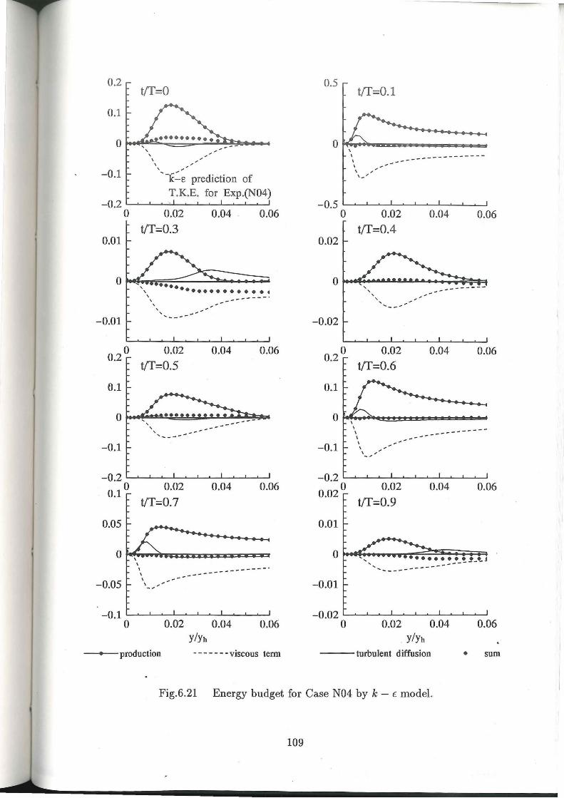
0.2 0.5 t/T=O t!f=O.l
0.1
0 0 \
/ / \ ----- ----------
/ \ /
\ ~-
-0.1 ' \ ' ~
'-k.::_E prediction of ,_,
T.K.E. for Exp.(N04) -0.2 -0.5
0 0.02 0.04 0.06 0 0.02 0.04 0.06
t/T=0.3 t!f=0.4 0.01 0.02
Fig.6.21 Energy budget for Case N04 by k - t model.
109

0.5 t/T=O
0 \ \ ~
\ ~
\ ~
\
'- /k-e prediction of T.K.E. for Exp.(N03)
-0.5 0 0.02 0.04 0.06
t/T=0.3 0.01
-0.01
0.2 0 0.02 t/T=0.5
0.06 0.04
-0.1 ' ~
0.04 0.06
0.05
------ ------0.05
-0.1 l_..,...___j.~--l..._._...J...._.....__.l..-..-.L__.__j
0 0.02 0.04 0.06 y/yh
--+--production - - - - - - - viscous term
0.5
0 I ------\ --- ----I
~ I ~
/ /
/ \ /
-0.5 0 0.02 0.04 0.06
t/T=0.4 0.02
-0.02
0.06 0.2 0 0.02 t/T=0.6
0.04
0.1
---- -----
-0.1 ~
~
-0.2 l_..,-.L__.___J__._......___.__L-..___.___.___J
0.02°
0.01
-0.01
0.02
t/T=0.9 0.04 0.06
-0.02 t_...____L__.__I.__.__.L...........___!.__.____,__.........__j
0 0.02 0.04 YIYh
---turbulent diffusion
0.06
• sum
Fig.6.22 Energy budget for Case N03 by k - t: model.
110

1
0.5
0 ~~~
"' "' -0.5
/
k -E prediction of /
I I
\I ,I T.K.E. for Exp.(N02)
-1 0 0.02 0.04 0.06
t/T=0.3 0.01
-0.01
0.04 0.06
0.1
-0.1
--------~~~
,,' ,.,"""'
/
-0.2 ._..___.___._---l.-__.__....___.o..____J._..___.___.___,
0.1°
0.05
-0.05 I
0.02
t/T=0.7
I , I ,
•/ ,,
0.04 0.06
----------~~~ ,--
-0.1 L--._.L.__._---l,___.__..J..._..........JL-o.---.1...__.___.
0 0.02 0.04 0.06 y/yh
---production - - - - - - - viscous term
0.5 t!f=O.l
0 \ ---- -------I ~~~
I "' I ' I /
,,1
-0.5 0 0.02 0.04 0.06
0.05 t!f=0.4
-0.05
0.2 0 0.02 t!f=0.6
0.04 0.06
0.1
-0.1
0.04 0.06
0.01
-0.01
-0.02 L--.---1..._.._--1.,._~L--..o.----'-_.._-'--~ 0 0.02 0.04
y/yh
---turbulent diffusion
0.06
• sum
Fig.6.23 Energy budget for Case N02 by k- c model.
111

1
-1
0
0.002
0.001
-0.001
o.oi
-0.02
0.05
-0.05
5
---asymmetric -------sinusoidal
t/(2tc)=t/T=O
t/(2tc)=t/T= 1/3
5
0.25 t(f, t/2tc
0.002
0.001
-0.05
0.01
0.005
0
-0.005
-0.01
2
0.5
t/(2tc)=t!f= l/12
t/ (2tc)=t!f = 1/4
t/(2tc)=t!f=5/12
-+--production viscous term Turb. Diff. sum (asymmetric) ·····+· .. ··production ······X······ viscous term ·· · ·· ·IJ··· · ·· Turb. Diff. ······ ·······sum (sinusoidal)
Fig.6.24 Comparison of k budget for asymmetric and sinusoidal cases by k - t model
under crest phase (As = 0.62).
112

1
0
-1 trough phase
0 0.25 t!f, t/2tt
0.005 0.004
0.002
0 0
-0.002
-0.005 -0.004
t/(2tt)=t!f = 1/6 0.05 0.02
0 0
-0.02 -0.05
0.05 t/(2tt)=t!f=l/3 0.01
-0.01 -0.05
5 10-2 2
y/yh
--+--production viscous term Turb. ..... + .. .. ·production .... .. x .... .. viscous term ...... a . ..... Turb.
0.5
t/(2tt)=t!f=l/12
t/(2tt)=t!f=1/4
5 10-2 2 5 10-1
y/yh
Diff. sum (asymmetric) Diff. ·· .. ··· ·· ···· sum (sinusoidal)
Fig.6.25 Comparison of k budget for asymmetric and sinusoidal cases by k- E model
under trough phase (As = 0.62).
113
2
6 .9 Conclusion
The following conclusions may be drawn from the present experimental study on asymmetric
oscillatory boundary layers;
1. An inexpensive piston movement system has been employed to generate asymmetric
oscillatory motion in an oscillating tunnel.
2. It was observed that the boundary layer thickness under trough is greater than that
under crest at high degree of asymmetry.
3. The generation and distribution mechanism of turbulence in asymmetric oscillatory
boundary layers is similar to that in sinusoidal ones except in the trough period, where
steady-like behavior was observed.
4. The wall shear stress profile during transition shows a bump in the deceleration phase
which is qualitatively similar to the behavior of sinusoidal oscillatory boundary layers
in transition.
5. The low Reynolds number k - t: model by Jones and Launder(1972) showed good
performance to predict mean velocity profile during acceleration phase, but during
deceleration phase its predictions were not satisfactory.
6. The overall agreement between the model prediction and experimental data is satis
factory for x direction fluctuating velocity.
7. The model overestimates the wall shear stress during deceleration phase but otherwise
its performance is satisfactory in this regard.
114
7 QUASI-STEADY OSCILLATORY BOUNDARY
LAYER ON A ROUGH BOTTOM
7.1 General
A precise estimation of sediment movement under long waves requires a correct choice of the
friction law out of wave and steady ones. In case of tsunami, the sediment movement was
studied by Takahashi et al.(1993), by using Manning 's equation, an equation applicable to
steady flows . Althou'gh, tsunami is a typical example of long wave, however, the long waves
do not exhibit quasi-steady properties of bottom friction under all the field conditions, so
that a steady friction law may be applicable. Therefore, for all the situations of a long wave,
utilization of steady friction law may yield unrealistic results. That is why it is necessary to
understand the behavior of the boundary layer during transformation from ordinary wave
to long wave.
In this case, probably the first theoretical and experimental study was carried out by
Yalin and Russell(1966) . They measured the velocities by a miniature current meter, there
fore no details about the turbulence structure could be obtained. Sawamoto and Hino(1977)
discussed the quasi-steady properties resulting from longer period of oscillation in case of a
laminar oscillatory pipe flow. They developed the relevant theory and carried out the experi
ments to validate it . Later Tanaka and Shuto(1994) extended this theory to a flat bottom and
developed the theory for rough turbulent wave motion on the basis of a time-independent
eddy viscosity model. They proposed the criterion to distinguish between ordinary and
quasi-steady wave boundary layers.
7.2 Rough Turbulent Flow
7.2.1 Basic equations
In case of steady turbulent flow over a rough surface, the velocity profile is expressed as ;
~ = ~ln (!!_) UJ K Yo
(7.1)
where; y0 denotes roughness height ( =Nikuradse's equivalent roughness/3D) and UJ is the
shear velocity. This is the so-called logarithmic velocity profile. This shape of profile exists
in the region where the momentum transport is independent of the viscous effects . Figure 7.1
shows the definition sketch for the different variables of logarithmic velocity profile, where y
is the cross-stream distance from theoretical bed level and z is the actual distance measured
from the top of roughness.
115

The friction factor for the present case is defined in usual way as;
To= ~fu~
where, u0 is the cross-stream average velocity.
z y t------_,
theoretical bed level is shown as y=O
Yo
u
Fig.7.1 Definition sketch for roughness.
7.2.2 Analytical model by Tanaka and Shuto(1994)
(7.2)
Tanaka and Shu to( 1994) used a linear eddy viscosity variation in cross-stream direction and
obtained the velocity profile and friction factor in terms of complex functions. They defined
the friction factor as follows;
(7.3)
where, u0 is the amplitude of cross-stream average velocity. This value, instead of the usual
value of velocity amplitude at the axis of symmetry, is used in order to facilitate its use in
ordinary as well as quasi-steady wave boundary layers. The friction factor thus obtained
depends on two dimensionless parameters, u0 j (wy0 ) and Yh / y0 , or collectively, as the.form
of these parameters suggests, on u0 jwyh .
By using.the similar eddy viscosity variation, the steady friction factor fc was given as;
(7.4)
116

a result slightly different from logarithmic friction law.
As a result of the computations by their model, Tanaka and Shuto(1994) proposed that
a wave boundary layer depicts quasi-steady behavior when;
Yh < 0.05 uo Yo - wyo
(7.5)
At this condition the difference between the friction factor computed from the exact
equation and the one for steady case was less than or equal to 10 percent.
7.3 Experimental Investigation
7.3.1 Experimental setup
The oscillating tunnel as described in Chapter 4 was used in the present set of experiments.
The bottom and top of the tunnel was roughened by using two dimensional triangular ele
ments. The height of the roughness elements was 5.4mm normal to the base of 10mm and
the spacing between them was maintained at 12mm. All the other experimental setup such
as the piston movement system and LDV system were same as described before.
The procedure for data analysis has also been presented in Chapter 4. In the present
series of experiments, it was necessary to find out the theoretical bed level and the theoretical
roughness height y0 • To achieve this , the method given by Jonsson(1963) has been utilized
here.
The experimental conditions for the cases presented herein are described in Table. 7.1,
where, the distance from theoretical wall to axis of symmetry Yh and cross-stream averaged
velocity u0 , the hat denotes amplitude of the quantity.
7.3.2 Velocity profile
In order to investigate the quasi-steady characteristics, detailed analysis has been presented
for the present experimental cases.
In Fig.7.2 to 7.8, where the value of u0jwyh ranges from 4.0 to 8.2, a prominent over
shooting of the velocity, which is a typical property of ordinary oscillatory boundary layers,
is evident. The thickness of the boundary layer, i.e. the distance from the wall to maximum
cross-stream velocity at wt = 0 (Jensen's definition) , increases gradually with the increase
in uofwyh value.
117

Table 7.1. Experimental conditions
Exp. ~T(ms) T(sec) v( cm2 / sec) Yo( em) uo( em/ sec) Uo fwyo Yh / Yo Jw Q01 10 4.86 0.0098 0.158 80.8 394.0 17.5 0.094
Q02 10 3.33 0.0104 0.130 36.8 149.0 21.3 0.119
Q03 10 5.39 0.0105 0.130 19.7 129.0 21.3 0.127
Q04 10 2.61 0.0106 0.130 55.4 175.5 21.3 0.111
Q05 10 3.52 0.0105 0.178 104.4 326.7 15.5 0.103
Q06 20 7.28 0.0098 0.163 50 .8 360.3 17.0 0.088
Q07 10 4.06 0.0100 0.174 100.8 372.8 15.9 0.093
Q08 20 5.5 0.0101 0.169 69.8 362.7 16.4 0.090
Q09 10 3.08 0.0104 0.167 145.4 426.5 16.6 0.097
Q10 20 4.32 0.0131 0.146 77.2 362.8 19.0 0.091
Q11 10 3.61 0.0145 0.142 81.9 329.6 19.5 0.091
Q12 10 3.57 0.0156 0.137 65 .6 270 .9 20.3 0.096
Q13 10 3.54 0.0157 0.130 50.0 215.3 21.3 0.104
Q14 10 3.55 0.0148 0.227 19.3 47.8 12.2 0.745
Q15 10 3.03 0.0104 0.161 27.2 81.0 17.2 0.195
Q1-6 10 2.56 0.0100 0. 160 36.0 92.0 17.4 0.177
Q17 10 3.52 0.0110 0.181 21.6 66.5 15.3 0.197
From Fig. 7.9 it may be observed that the thickness of the boundary layer is considerably
increased until it reaches the axis of symmetry in Fig.7.10 , where the value of u0 j wyh is 13.4.
In the next figures (7.11 to 7.18), the boundary layer thickness remains equal to Yh· In other
words , the overshooting which was observed in the previous cases, does not exist anymore.
The velocity profile at every phase resembles that of a steady flow, except in the vicinity of
wt = 7r / 2, the reason why this type of oscillatory boundary layer is called as quasi-steady
oscillatory boundary layer.
A collective view of the figures 7.2 to 7.18 shows that the phase difference near the wall,
which is a typical oscillatory boundary layer property, gradually decreases with the increase
in uo/ WYh ·
The quasi-steady property is generally depicted by long period waves, but as can be seen
from the present experiment, only period of oscillation is not sufficient to classify the flow
as quasi-steady, for example the period of oscillation for Q03 (Fig.7.6) is longer as compared
to that for Q09 (Fig. 7.18), but the quasi-steady properties are shown by Q09. This confirms
the findings of·Tanaka and Shuto(1994) that for rough turbulent wave boundary layers, the
distinction between ordinary and quasi-steady wave boundary layers can be made by the
parameter uo / WYh·
118

2
1
-20 0 u(cm/sec)
Fig.7.2 Velocity profile for case Q14(u0j wyh = 4.0).
. -20 0 u(cm/sec)
20
Fig.7.3 Velocity profile for case Q17(u0j wyh = 4.3).
119
20

2
1
-20 0 u(cm/sec)
20
Fig.7.4 Velocity profile for case Q15(u0jwyh = 4.7).
-40 -20 0 u(cm/sec)
20
Fig.7.5 Velocity profile for case Q16(u0jwyh = 5.3).
120
40
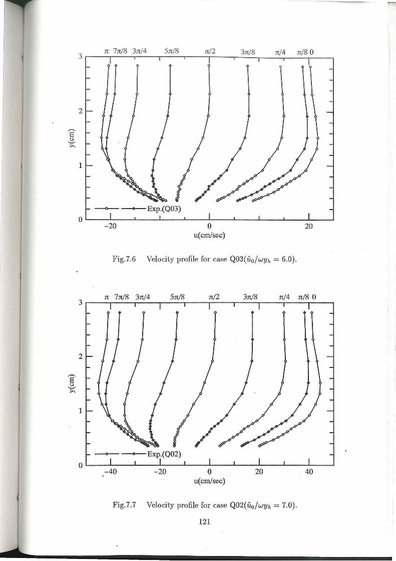
rc 7rc/8 3rc/4 Src/8 rc/2 3rc/8 rc/4 rc/8 0 3r---.----.----r---.---~----.---~--~----~--~
2
1
-20 0 u(cm/sec)
Fig.7.6 Velocity profile for case Q03( u0 jwyh = 6.0).
-40 -20 0 u(cm/sec)
20
Fig.7.7 Velocity profile for case Q02(uo/wyh = 7.0).
121
20
40
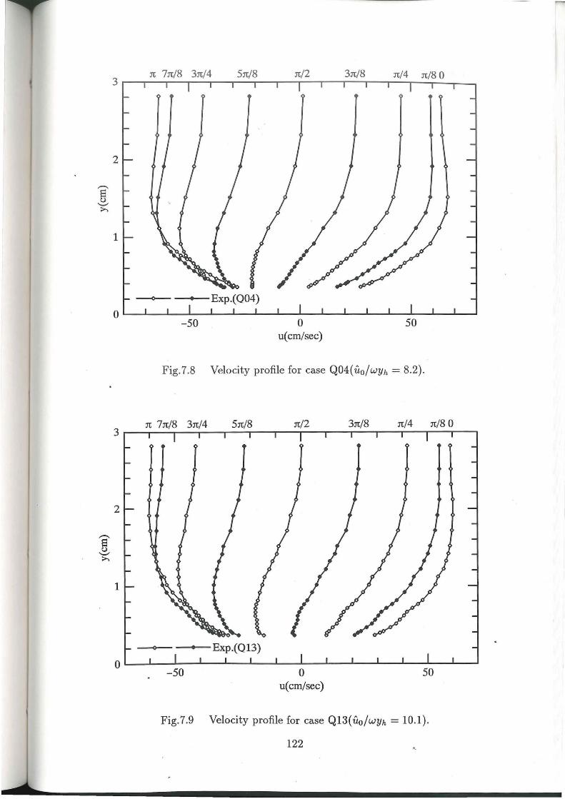
2
1
-50 0 u(cm/sec)
50
Fig.7.8 Velocity profile for case Q04(u0jwyh = 8.2).
0~~--~--~--L-~~~--~--~--L-~--_.--~--._~
-50 0 50 u(cm/sec)
Fig.7.9 Velocity profile for case Q13(u0jwyh = 10.1).
122 ..
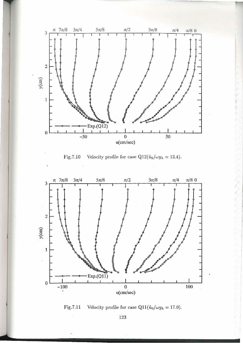
2
1
-50 0 u(cm/sec)
50
Fig.7.10 Velocity profile for case Q12( u0jwyh = 13.4) .
5n/8 n/2 3n/8 n/4 n/8 0
-100 0 u(cm/sec)
Fig.7.11 Velocity profile for case Qll(u0jwyh = 17.0).
123
100

2
1
-100
2
1
Sn/8 n/2 3n/8 n! 4 n/ 8 0
0 u(cm/sec)
Fig.7.12 Velocity profile for case Q10( u0 jwyh = 19.0).
-100 0 u(cm/sec)
Fig.7.13 Velocity profile for case Q05(u0jwyh = 21.0).
124
100

-100
-50 0 u(cm/sec)
50
Fig.7.14 Velocity profile for case Q06(u0j wyh = 21.1).
0 u(cm/sec)
Fig.7.15 Velocity profile for case Q08( u0j wyh = 22.0).
125
100
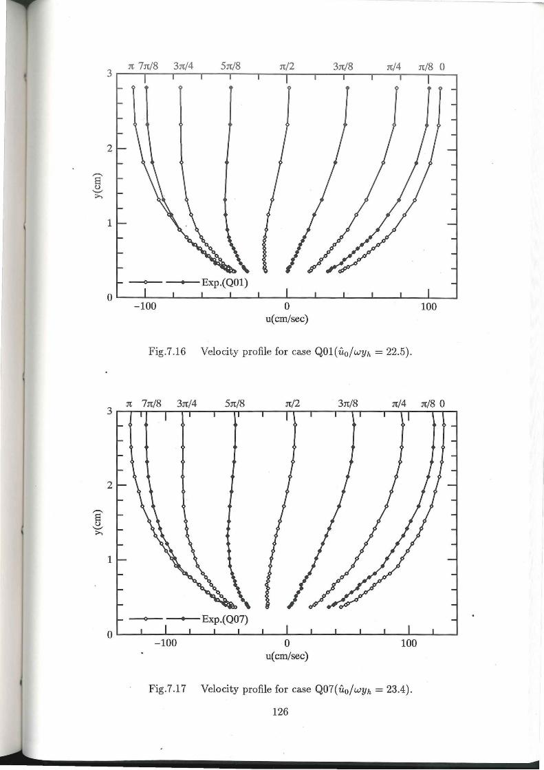
2
1
-100 0 u(cm/sec)
Fig.7.16 Velocity profile for case Q01(u0jwyh = 22.5).
-100 0 u(cm/sec)
100
Fig.7.17 Velocity profile for case Q07( u0j wyh = 23.4).
126
100

2
1
0~----~----~----~----~~----~----~----~----~ -200 0
u(cm/sec)
Fig.7.18 Velocity profile for case Q09( u0jwyh = 25.7).
7.3.3 Mean velocity amplitude and phase difference
200
In order to comprehend the gradual transformation of ordinary wave boundary layer to
quasi-steady one, an overview of the cross-stream profiles of mean velocity amplitude and
phase difference would be of interest. As mentioned earlier the discriminating factor may be
the parameter u0 /wYh· That is why the relevant figures in this subsection are also arranged
in ascending order of the value of uo/WYh·
Figure 7.19 shows the profile of mean velocity amplitude and the phase difference for
the case in which the value of u0jwyh is very small(=4.0). The velocity overshooting and
its weak damping in cross-stream direction towards axis of symmetry is clearly visible. This
weak damping may be observed in the profile of phase difference also. This property is
typical in the ordinary oscillatory boundary layers.
As the value of u0jwyh increases gradually in the subsequent figures (Fig.7 .20 to Fig.7 .25),
the weak damping in the phase difference as well as velocity amplitude profile goes on dimin
ishing. The velocity overshooting tends towards the axis of symmetry, or in other words the
thickness of boundary layer goes on increasing. In Fig. 7.26 the velocity overshooting seems
to be very mild ail.d stretched in the cross-stream direction. The phase difference profile
shows a reverse tendency near the wall. This tendency is clearly observed in Fig.7.27 and
127

Fig. 7.28 also . In these figures , as may be observed the boundary layer thickness is nearly
equal to Yh· In Fig.7.29 the phase difference profile near the wall becomes almost vertical.
The boundary layer thickness becomes equal to Yh as shown by the velocity amplitude pro
file. In Fig.7.30 and Fig.7.31, where the value of u0jwyh is nearly the same( = 21), it may
be noted that the profiles of velocity amplitude and phase difference show almost similar
behavior, though the free-stream velocity is much different in these two cases. It may be
noted that the range of phase difference from the wall to axis of symmetry is also about the
same in both these cases.
Further increase in u0jwyh does not change the behavior of velocity amplitude profile
in the cross-stream direction. But the range of phase difference from the wall to axis of
symmetry goes on becoming narrow as is obvious from Fig.7.32 to Fig.7.35. This decrease
in phase difference near the wall may be attributed to an increase amount of momentum
transport from the high velocity regions.
In order to further elucidate what has been described before, the velocity amplitude and
phase difference profiles of selected cases are plotted in Fig.7.36 and Fig.7.37, respectively.
It may be observed that the demarcation between ordinary oscillatory boundary layers and
quasi-steady ones rhay lie in between u0jwyh = 8.2 to 10.1 , as the quasi-steady effects emerge
just after uo f wyh = 8.2.
7.3.4 Turbulence intensity
In order to observe the difference of behavior in turbulence intensity for the present cases,
the fluctuating component of the velocity u' is presented here. As is obvious from Fig. 7.38
to 7.45, the fluctuating velocity shows the generation of turbulence in the near wall region
during the deceleration phase and its gradual spreading in cross-stream direction during
acceleration phase. The phase difference in normal direction to the wall is obvious in these
cases. This is the usual property of ordinary wave boundary layers, as shown by previous
researchers experimentally as well as numerically (see e.g. Jensen, 1989, Justesen, 1988) and
in the present study( see Chapter 3 and 4), regardless of the wall condition, whether smooth
or rough.
In Fig.7.46 to 7.54, the situation is rather different, here, the phase difference in normal
direction no longer exists. Moreover, the magnitude of turbulence fluctuations is quite large
near the axis of symmetry as compared to that in previous cases (Fig.7.38 to 7.45). The
reason being significant magnitude of mean velocity gradient which is responsible for the
production of turbulence, at the axis of symmetry in these cases. A constant u' layer can be
observed near the.wall, during the maximum free-stream velocity phases.
128

e(deg)
-20 0 20 40 3r· --,---~--~--r--,--~---r---r--,---~--~~~~
2
,..__ 5 "-" >-.
1
--o---
---o--
0 0 10 20 30
fi(cm/sec)
Fig.7.19 Velocity amplitude and phase difference profile at u0 jwyh = 4.0 (Q14).
6(deg)
2
,..__ 5
"-" >-.
1 Exp. (Q17)
--o--- ft
---o-- e
0 0 10 20 30
fi(cm/sec)
Fig.7.20 Velocity amplitude and phase difference profile at u0jwyh = 4.3 (Q17).
129

6(deg)
2
-. 5 '-" >.
1
~ ft
~ e
0 0 10 20 30
u(cm/sec)
Fig.7.21 Velocity amplitude and phase difference profile at u0 jwyh = 4.7 (Q15).
6(deg)
2
-. 5 '-" >.
1 Exp. (Q16)
~ ft
~ e
0 0 20 40
u(cm/sec)
Fig.7.22 Velocity amplitude and phase difference profile at u0jwyh = 5.3 (Q16).
130
d
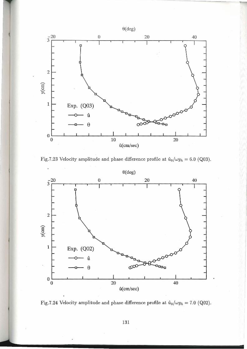
8(deg)
2
,-...
§ '-" >.
1 Exp. (Q03)
--o-- fi
~ e
0 0 10 20
u(cm/sec)
Fig.7.23 Velocity amplitude and phase difference profile at u0 jwyh = 6.0 (Q03).
8(deg)
2
,-...
§ '-" >.
1 Exp. (Q02)
--o-- fi
~ e
0 0 20 40
u(cm/sec)
Fig.7.24 Velocity amplitude and phase difference profile at uo / WYh = 7.0 (Q02).
131

2
1 Exp. (Q04)
-o-- ft
20
6(deg)
40 u(cm/sec)
60
Fig.7.25 Velocity amplitude and phase difference profile at u0jwyh = 8.2 (Q04).
6(deg)
-20 0 20 40 3~~--~--~--~--~--~--~~--~--~--~--~~
2
1 Exp. (Q13)
-o-- ft
o~_.--~--~~--~--~--~_.--~--~~~~--~~
0 20 40 u(cm/sec)
60
Fig.7.26 Velocity amplitude and phase difference profile at uo /WYh = 10.1 (Q 13).
132

e(deg)
-20 0 20 40 3~--~~~~--~---T---r---r--~--~--~--T---~--
2
1 Exp. (Q12)
~ft
--o-- e
0~--~-----L----~----~--~~--~----~----~--~ 0 20 40
u(cm/sec) 60 80
Fig.7.27 Velocity amplitude and phase difference profile at u0 jwyh = 13.4 (Q12) .
8(deg)
2
..-5 '-' >.
1 Exp. (Qll)
~ ft
--o-- e
0 0 50 100
u(cm/sec)
Fig.7.28 Velocity amplitude and phase difference profile at u0jwyh = 17.0 (Qll).
133
~-· ------------------------~rl

8(deg)
-20 0 20 40 3~~--~--~--~--~--~--~~~----~--~--~~
Exp. (QlO)
---o-- u
50 fi(cm/sec)
100
Fig.7.29 Velocity amplitude and phase difference profile at u0 jwyh = 19.0 (Q10) .
2
-.. ~ ._. >.
1
0 0
-20
Exp. (QOS)
---o-- u --o-- e
50
8(deg)
0
fi(cm/sec) 100
20
150
Fig.7.30 Velocity amplitude and phase difference profile at u0jwyh = 21.0 (Q05).
134

2
1 Exp. (Q06)
-o-ft
--o-- e
20
6(deg)
40 u(cm/sec)
60
Fig.7.31 Velocity amplitude and phase difference profile at u0 jwyh = 21.1 (Q06) .
6(deg)
20 40
2
1 Exp. (Q08)
-o-ft
--o-- e
0~--~----~--~----~--~----~--~----~--~--~ 0 20 40 60 80 100
u(cm/sec)
Fig.7.32 Velocity amplitude and phase difference profile at u0jwyh = 22.0 (Q08).
135

8(deg)
2
,-.
5 '-' >.
1 Exp. (QOl)
--o-- ft
-o-- e
0 0 50 100
u(cm/sec)
Fig.7.33 Velocity amplitude and phase difference profile at u0 jwyh = 22.5 (QOl).
8(deg)
2
,-.
5 '-' >.
1 Exp. (Q07)
--o-- ft
-o-- e
0 0 50 100
u(cm/sec)
Fig.7.34 Velocity amplitude and phase difference profile at u0jwyh = 23.4 (Q07) .
136

6(deg)
2
,.-.._
5 '-' ::>.
1
--o-- u ---o- e
0 0 50 100 150 200
u(cm/sec)
Fig.7.35 Velocity amplitude and phase difference profile at u0 jwyh = 25.7 (Q09) .
7 .3.5 Momentum balance
Another interesting property of quasi-steady boundary layer is regarding the momentum
balance. For the present case of one-dimensional unsteady flow in x direction, the momentum
equation has been given in Chapter 3 (Eq.3.1 ).
Integrating this equation from the wall to the axis of symmetry and dividing throughout by
u5, we get the following dimensionless equation,
Yh auo 1 [Yh ap d To u6 at = - pu6 Jo ax y - pu6 (7.6)
'--v--" "-v-" I II III
Here, pis the pressure and To wall shear stress. The terms I, I I and I I I may be called as
acceleration, pressure gradient and shear term, respectively.
A~ explained by Yalin and Russell(1966), the acceleration term vanish in case of quasi
steady wave boundary layer. In the present study, term I can be obtained by differentif.ting
the cross-stream averaged velocity u0 with respect to time, and term I I I can be obtained by
assuming logarithmic velocity profile near the wall, term I I is determined by using Eq.(7.6).
In figures 7.55 to 7.58, it may be observed that the shear term exceeds the acceleration
term to much extent, which is in accordance with what Yalin and Russell(1966) have shown
137

theoretically.
4.3 6.0 8.2 10.1 13.4 17.0 19.021.023.4 25.7
..c:: ~ 0.5
o~~~~~~~~~~~~~~~~~~~~~~~~~~
..c::
0 0
uofwyh=
0 0 0 0 0 0 fi/fio
0 0 0.5
Fig.7.36 Velocity amplitude profiles of selected cases.
4.3 6.0 8.2 10.113.4 17.ol9·0 21.0 23.4 25.7
1 1.5
1~~~~~~~~~~~~~~~~~-T-r~~~~~~~
~ 0.5
o~~~~--~~~--~~~--~~--~---L~~--~~~~ -20 0 0 0 0 0 0 0 0 0 0 20
6(deg)
Fig.7.37 Phase difference profiles of selected cases.
138

Q14
2.50 u'(cm/sec)
2.00
1.00 ---
s () 1. 50 <>
........... :>...
1.00
0 .00 0 .20 0 .40 0 .60 0 .80 t / T
Fig. 7.38 Contours of fluctuating velocity for case Q14( uofwyh = 4.0).
Q17
2.50 u'(cm/sec)
2.00
1.0
0.5
0 .00 0 .20 0 .40 0 .60 0 .80 t / T
Fig. 7.39 Contours of fluctuating velocity for case Q17( u0jwyh = 4.3).
139

Q15
0 2.50
2 .00
1.00
0 .50
0 .00 0. 20 0 .40 t / T
0 .60 0 .80
Fig.7.40 Contours of fluctuating velocity for case Q15(u0jwyh = 4.7) .
2 .50
2 .00
1.5
0 .00
c§J ~ -
Q16
u'(cm/ sec)
~200
0 .20 0 .40 t / T
0 .60 0 .80
Fig.7.41 Contours of fluctuating velocity for case Q16(u0jwyh = 5.3) .
140

Q03
2. 50 \]
2.0 0 9
u'(cm/ sec)
s u 1.50
'--' :>,
1.00
0.00 0 .20 0 .40 t / T
0 .60 0 .80
Fig. 7.42 Contours of fluctuating velocity for case Q03( u0 jwyh = 6.0).
2.50
2.0
s u 1.5
'--"' :>,
1.0
0 .50
0.00 0 .20 0 .40
Q02
u'(cm/ sec) 0
t / T
~2.0 2-T-~o . ~
3.0
0 .60 0.80
Fig.7.43- Contours of fluctuating velocity for case Q02(u0/wyh = 7.0).
141
5
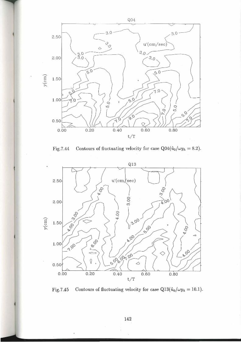
Q04
0 .00 0.20 0 .40 0.60 0.80
t / T
Fig.7.44 Contours of fluctuating velocity for case Q04(u0jwyh = 8.2).
Q13
0.40 0 .60 0 .80 t / T
Fig.7.45 Contours of fluctuating velocity for case Q13(u0jwyh = 10.1).
142

Q12
0 .00 0 .20 t / T
Fig.7.46 Contours of fluctuating velocity for case Q12(u0jwyh = 13.4).
Qll
0 .00 0 .20 0 .40 0 .60 0 .80 t / T
Fig. 7.47 Contours of fluctuating velocity for case Qll( uo /WYh = 17.0).
143

QlO
0.00 0 .20 t / T
Fig. 7.48 Contours of fluctuating velocity for case QlO( u0 jwyh = 19.0).
3.00
,_.. a a a
·a rna a a
Q05
m ·a
CP a a a
s C) 1.5 ...__..-:>..
0.20 0 .40 t / T 0 .60 0.80
Fig.7.49 Contours of fluctuating velocity for case Q05(u0jwyh = 21.0) .
144

Q06
3 .00
2.50
2. 00
s ._S 1.50
p...
1.00
0.20 0.40 t / T
0.60 0.80
Fig.7.50 Contours of fluctuating velocity for case Q06(u0/wyh = 21.1).
Q08
C")
(Jl
2.50
~ ..-.._
0 s 0 () lD.
'-" p...
co
0.00 0.20 0 .40 0 .60 0 .80
t / T
Fig.7.51 · Contours of fluctuating velocity for case Q08(u0jwyh = 22.0).
145

QOl
0.00 0 .20 0 .40 t / T
Fig. 7.52 Contours of fluctuating velocity for case QOl( u0 jwyh = 22.5).
Q07
0 .00 0 .20 0 .40 0 .60 0.80
t / T
Fig.7.53 Contours of fluctuating velocity for case Q07(u0jwyh = 23.4).
146

Q09
0 .5
t / T 0 .60
Jso
) <:.0 0 0
0 .80
Fig. 7.54 Contours of fluctuating velocity for case Q09( u0 jwyh = 25. 7).
In an oscillating flow with potential flow region (vertical cross-stream velocity profile),
for a certain value of the acceleration term, the pressure term is balanced by the shear term.
Since in the present case, roughness is very high, therefore the produced wall shear stress is
very high in magnitude.
Figures 7.59 to 7.61 clearly show that , the shear term is much less as compared to
acceleration term, thus supporting the assumption of inviscid flow in most of the coastal
environments, where, the boundary layer thickness is very small as compared to the distance
between solid and free-stream boundaries. Here, the acceleration and pressure terms are
important, i.e. by magnitude I~ II> III.
The Fig.7.62 to 7.71 which are relevant to the quasi-steady cases as has been shown by
C velocity profiles, thickness of the boundary layer is equal to the flow depth so shear term
can no longer be neglected. The acceleration term is small as compared to the other two
terms in this condition, i.e. by magnitude I < II ~ II I . It may be anticipated that
as the parameter u0jwyh would increase, the contribution of the acceleration term in the
momentum balance will decrease further.
In order to get an overall observation of the momentum balance shown previously., the
maximum values of acceleration, pressure and shear terms are plotted in Fig.7.72. As may
be noted from this ~gure , for low values of uo fwyh, the shear term produced by the roughness
has high magnitude which must be balanced by the pressure term. With a furhter increase
in the uo/WYh value, the boundary layer thickness approaches the axis of symmetry. The
147

shear term in this situation decreases and larger part of the pressure term is balanced by
the acceleration term.
...... ...... ......
...... ......
0.5 r----y-----,---r-----,---~-.....,---.,r----r---y----.,
...... ...... ...... <>(j ...... ...... ...... ~
··. · .
0.1
0
-0.1
. ... ····......... .· .. ... ··.·.•. .-
.,._,.···~--....r·· Exp.( Q 14)
0.5 t!T
.· .... ... ··
___ ............... ~ . ., .. ... . •
1
Fig.7.55 Momentum balance at u0 jwyh = 4.0 (Q14).
---1 (acceleration)
······ ······· II (pressure)
-·-III (shear) /·.,--·-......_.
. "' .// ""
.· ·······.;····... . ............... ···
·· ..... . .·· ·····... . .... ·· ···········
Exp.(Q17)
.. ···· ..·· . .
.. ····· ········· .····
-0.2~--_.----~--~----~--~~--~----~--~----~--~ 0 0.5
t!T
Fig.7.56 Momentum balance at u0jwyh = 4.3 (Q17).
148
1

-----
---c:-6 ---~
c
0.1
-0.1
---I (acceleration)
· · · · ·· · · · · · · · II (pressure)
-·-III (shear) / . ...-.-.,. /. """· ./·
··· ... ...·· ······ .. ·····... .··· .... ··· ............... ··
Exp.(Q15)
....... ····· .. .· ·. ..················ ~ .. ;
-0.2 L....----'---L....----'---..___---'-__ ..____--'---"------'----J
0
0.1
0
-0.1
0.5 t!f
Fig.7.57 Momentum balance at u0jwyh = 4.7 (Q15).
---I (acceleration)
···· ···· ····· II (pressure)
-·-III (shear)
..,--. """'""-."""' /" .,
..
./· "· ~-:-----~
···· ... ·······... ..
···. ..···· ····· ........... :
0.5 t!f
Exp.(Q16)
Fig.7.58 Momentum balance at uo/WYh = 5.3 (Q16).
149
1
1

0.1
....... ....... .......
Qd 0 ....... ....... .......
-0.1
0.1
....... ....... .......
ctd 0 ....... ....... .......
(
-0.1
0
---1 (acceleration)
· · ·· · · · ·· ·· ·· II (pressure)
-·-III (shear)
.... ... · .... -~ ·: ~
····· ........ :
... :"'
... . -
0.5 t!f
Exp.(Q03)
Fig.7.59 Momentum balance at u0 jwyh = 6.0 (Q03).
---1 (acceleration)
·· ··· · ··· · ·· · II (pressure)
-·-III (shear)
0.5 t!f
Exp.(Q02)
.""" ·"""· --·
Fig.7.60 Momentum balance at u0jwyh = 7.0 (Q02).
150
1
1

0.1
-----
-0.1
0
0.05
-----
-0.05
0
---I (acceleration)
· · ·· · · · ·· · · · · II (pressure)
-·-III (shear)
. •
........ ········· Exp.(Q04)
0.5 t!T
"""' ·""-.. --. .
Fig.7.61 Momentum balance at u0 jwyh = 8.2 (Q04).
---I (acceleration)
·············II (pressureJ..r""""\..."
-·-III (shear)./ ·\.
I . ;·
··· .. ··. ··... _, ... ·
·. . ... .......... · .··
0.5 t(f
Exp.(Q13)
... ······· ........ . ....... · ..
.· ... ····
Fig.7.62 Momentum balance at u0jwyh = 10.1 (Q13).
151
1
1

---c:d --........
-----
0.05
0
-0.05
0
0.05
--I (acceleration)
············· II (pressure) . ....,-.""""·
-·-Ill (shear)./ "'-.'\...
.1 . ·· ... I
. .....
......
... :" ... ··
·····-~.····--~· Exp.(Q12)
0.5 t(T
.· .. ···· ..
_.,. ... ···--.... _ .... ····· ······· ..
Fig.7.63 Momentum balance at u0jwyh = 13.4 (Q12).
--I (acceleration) ·~
·············II (pressurey .,.
···... -·-III (shear~/ '\
I . . "' .
1
··. ;· . X. o~----4-~~~·----------~----~~:--~~--------~
-0.05
0
.·
. ··· ..
·············... _... /.··Exp.(Qll)
··· ..... -········
0.5 t(T
Fig.7.64 Momentum balance at u0jwyh = 17.0 (Qll ).
152
1

-----
-----
0.05
-0.05
0
0.05 .
-0.05
0
··· ... .. ·· ..
---I (acceleration)
· · ·· · · · ·· · · · · II (pressure) . .,.._,.,.,._,.. -A....r
-·-III (she//'" ·"\..
I
~·
...... .... ·····-·,··-
Exp.(QlO)
0.5 t(f
.. ... ·· .· ...... ············· .......... · .. .
Fig.7.65 Momentum.balance at u 0 jwyh = 19.0 (Q10).
---I (acceleration)
· · ·· · · · ·· · · · · II (pressure) . ~. -·-. III (shear) ./ """·"'-.
I . ·· ... ;·
.· ... · .·· .··· ············· Exp.(QOS)
0.5 t(f
... ············ .. · .... ..··· .
.... ····
Fig.7.66 Momentum balance at u0j wyh = 21.0 (Q05).
153
1
1
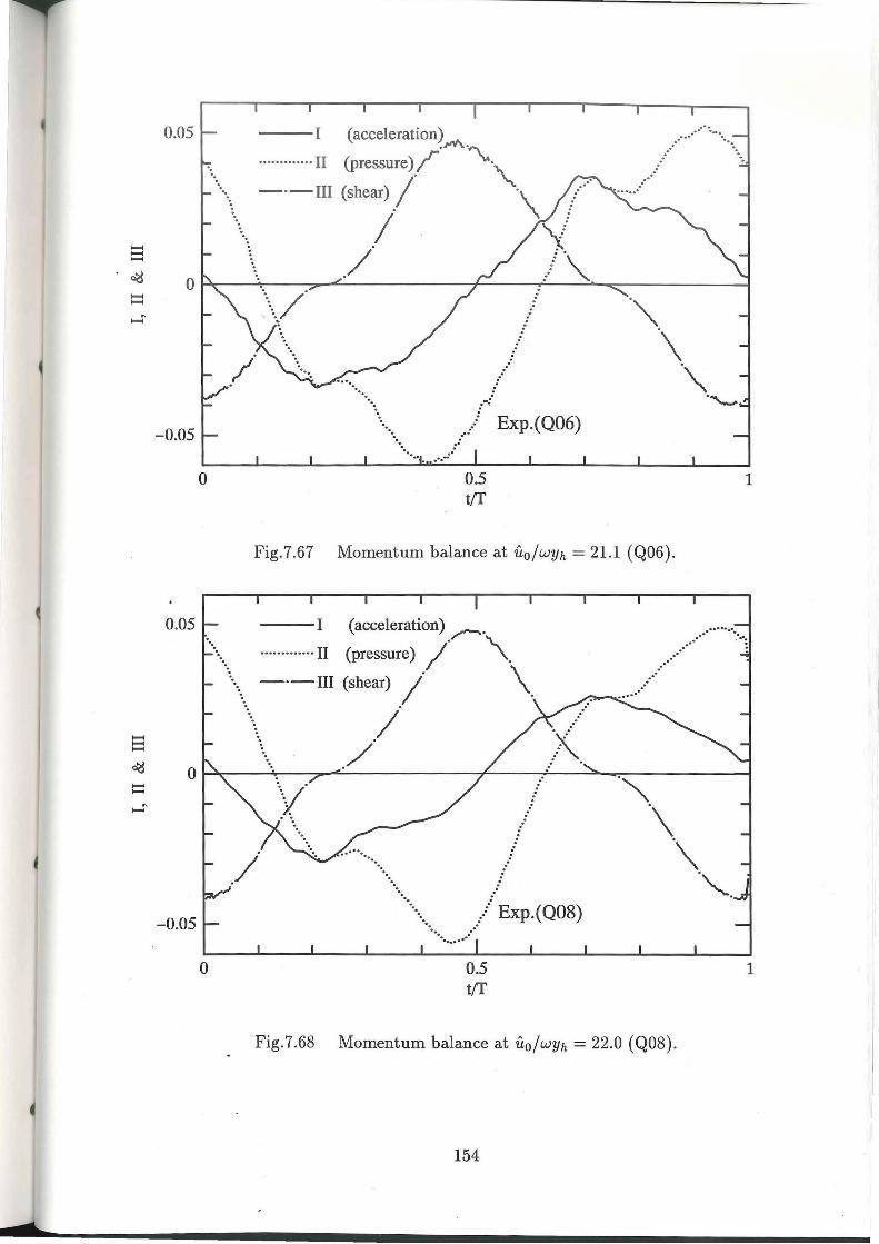
-----
-----
0.05 --I (acceleration) ·""'·""
·············II (pressure)./ "'·"
- ·-III (shear)./ ·\ .
. 1 \:· / /.
..·· ......
... ... ········· ·-· ...•...
.·· ·.
. ... " 0~--~·--~--~----------r---~~--~~--------~
-0.05
0
0.05
···· .. ··· ...
·· ... 0.5 t{f
Exp.(Q06)
Fig.7.67 Momentum balance at u0 .fwyh = 21.1 (Q06).
--I (acceleration),.,-....
············· II (pressure) ;· "\..
-·-III (shear) ;· \.
;·
1
./ 0~----~~~~----------~--~~--~-----------~
" .\ -0.05
0
········· ... ····· ...
··········... .. ..... / Exp.(Q08) · ...... .
0.5 t{f
." .,.
Fig.7.68 Momentum balance at u0jwyh = 22.0 (Q08).
154
1

---<>'d --.......
--
0.05 I (acceleration)
0
-0.05
0
0.05
. ...-.""' ············· II (pressure) / '·
-·-III (shear) ./· \.
/ .1·
.. .~·
/Exp.(QOl) ..... ······ ........... :·
0.5 t!f
Fig.7.69 Momentum balance at uo/WYh = 22.5 (QOl).
---I (acceleration)
· · ·· · · · ·· · · · · II (pressure)_./""""·"""""-. ..........,.
··~.\-·-III (shear)./ .,.
1
I .I
o~~--~--~~--------~~~----~--~~--------~ .\
-0.05
0
.. . ~· .....
"
-··· .... ··············· Exp.(Q07)
0.5 t!f
\ ."'
Fig.7.70 Momentum balance at uo/WYh = 23.4 (Q07).
155
. """"'-.
1

-----
0.05 ---I (acceleration)
············· II (pressure);·-"·"""·
.-·-111 (shear);· "\ ·. . '\ ........ I .
........... ··
... ···
.. ·············· ....
· .. \ /. 0. ~------~--~~---------=~------~~~~----------~
-0.05
0
.. . ••·······•••. . .. · :
...... · ··.. .:··· Exp.(Q09) ......... ·
0.5 t(f
Fig.7.71 Momentum balance at u0 jwyh = 25.7 (Q09).
1
For guite high magnitude of u0 jwyh, the boundary layer thickness becomes equal to
Yh, i.e. quasi-steady condition is reached and the acceleration term is decreased further as
compared to other terms.
7 .3.6 Friction factor
Tanaka and Shuto(1994) showed by their model predictions that as the parameter uo/WYo
increases for a certain value of Yh/Yo , the friction factor tends towards a value determined
from steady friction law and it no longer depends on u0 jwy0 after crossing a certain limit.
Figure 7.73 shows the experimental data by Yalin and Russell(1966) along with the model
predictions by Tanaka and Shuto(1994) . It may be observed that the experimental data
shows a similar trend as predicted by the model. Although the data scatter is considerable,
however, variation of the friction factor to become independent of the parameter uo/wyo
seems to be quite obvious. The Eq.(7.5) has also been shown. It might be noted that the
value of Yh/Yo( =1110) for the experimental data by Yalin and Russel1(1966) is quite high
as compared to the present experiments. For the present series of experiments, Fig. 7. 7 4 has
been plotted. The wave friction formula by Jonsson(1963);
1 1 ( u0 ) 4ffw + logto 4ffw = -0.08 + logto 30wyo (7.7)
156
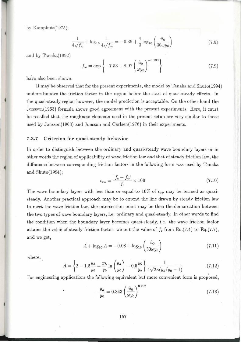
by Kamphuis(1975);
1 1 4 ( u0 )
T + log10 rr = - 0.35 + - log10 --
4y Jw 4y fw 3 30wyo (7.8)
and by Tanaka(1992)
{ (
~ ) -0.100}
fw = exp - 7.53 + 8.07 ::0
(7.9)
ha~e also been shown.
It may be observe,d that for the present experiments, the model by Tanaka and Shuto(1994)
underestimates the friction factor in the region before the start of quasi-steady effects. In
the quasi-steady region however, the model prediction is acceptable. On the other hand the
Jonsson(1963) formula shows good agreement with the present experiments. Here, it must
be recalled that the roughness elements used in the present setup are very similar to those
used by Jonsson(1963) and Jonsson and Carlsen(1976) in their experiments.
7.3.7 Criterion for quasi-steady behavior
In order to distinguish between the ordinary and quasi-steady wave boundary layers or in
other words the region of applicability of wave friction law and that of steady friction law, the
difference. between corresponding friction factors in the following form was used by Tanaka
and Shuto(1994);
Ecw = ifc - fw i X 100 fc
(7.10)
The wave boundary layers with less than or equal to 10% of Ecw may be termed as quasi
steady. Another practical approach may be to extend the line · drawn by steady friction law
to meet the wave friction law, the intersection point may be then the demarcation between
the two types of wave boundary layers, i.e. ordinary and quasi-steady. In other words to find
the condition when the boundary layer becomes quasi-steady, i.e. the wave friction factor
attains the value of steady friction factor, we put the value of fc from Eq.(7.4) to Eq.(7.7),
and we get,
where,
A + log10 A = - 0.08 + log10 ( Ouo ) 3 wyo
A = { 2 _ 1.5 Yh + Yh ln (Yh) _ O.S Yo} 1 Yo Yo Yo Yh 4vf2,;;,(yh/Yo - 1)
(7.11)
(7 .12)
For engineering applications the following equivalent but more convenient form is proposed,
( ~ )0.797
Yh = 0.343 uo Yo wyo
(7.13)
157

---I (acceleration)
-------II (pressure) 0.3
----III (shear)
---<>Cl 0.2 --
0.1
10 20 30
Fig.7.72 The maximum values of acceleration, pressure and shear terms.
0 Yalin and Russell(1966)
---Tanaka and Shuto(1994)
-·-Eq.(7.5)
0
8 oco
y.Jy0=1110
Fig.7.73 The variation of friction factor for the experiment by Yalin and Russell(1966).
158

5
Tanaka(1992) --- theory(Tanaka & Shuto,1994)
• 0
*
Kamphuis(1975) Jonsson(1963)
iio/ooyo>175 r iio/ooy0<175 resent Exp. steady flow
10-2 ~------~--~--~~~~~~------~--_.--~_.~_.~~ 1~ 1~ 1~
uof(myo)
Fig.7.74 Friction factor diagram for the present experiments.
Fig.7.75 shows the results of the model by Tanaka and Shuto(1994) for Ecw values of
1, 5 and 10 percent. It might be observed that the original criterion proposed by Tanaka
and Shuto(1994) shows little discrepancy for low values of Yh / Yo whereas the new criterion
is applicable to almost whole the range of parameters. Especially, for low values of Yh / Yo as
that for the present experiment, the present criterion distinguishes between the two zones
of applicability of wave and steady friction laws in an excellent manner. For the present
experiment, the value of Yh / Yo is about 21 on the average. For this value, as may be
obtained from Eq.(7.13), the data points having u0 j wy0 equal to or greater than 175 show
quasi-steady behavior. It may be noted from a collective observation of Fig.7.74 and Fig.7.75
that the present criterion Eq.(7 .13) show the demarcation between ordinary and quasi-steady
boundary layers.
7.4 A Practical Example of Quasi-Steadiness
In order to elucidate the importance of the criterion for inception of quasi-steadiness, the
computation was made by using the theory of Tanaka and Shuto(1994), for two typical
cases of wave propagation one with a period of 10 minute(Case 1) and another with that
of 10 second(Case 2). The bed slope was kept as 1/ 100 and wave height, H = 1m at
159

Yh = lOOm for both the cases. A uniform sand roughness with y0 = l cm was assumed. The
schematic sketch for this example is shown in Fig.7 .76. For the wave shoaling, the theory by
Shuto(1974) was employed. The breaking point(BP) was determined using the breaker index
by Goda(1975) and after breaking point the wave height was assumed to decrease linearly
towards shoreline. The boundary layer thickness b is defined as the distance from bed to
maximum cross-stream velocity location (definition by Jensen,1989) and it was computed by
using the empirical formula given by Sana and Tanaka(1995) . The critical point(C.P.) is that
corresponding to the criterion to distinguish between ordinary and quasi-steady boundary
layers(Eq.(7 .13) ).
As shown for Case 1 in Fig.7.77, which is a typical example of long wave as the Yh/ L
(L =wave length) remains well below 1/25, when waves propagate towards the shoreline,
they undergo shoaling process, i.e. the wave height increases. Initially, the wave friction
law is applicable, and then at the critical point (C.P.) where wave boundary layer thickness
b according to Jensen(1989) definition (the distance from the bottom to maximum cross
stream velocity at wt = 0) becomes equal to the depth of flow Yh, the zone of applicability of
steady friction law begins. It must be noted that the boundary layer under this wave with
a period of 10 minute might be mistakenly taken as a quasi-steady one. But the present
computations show that this happens only within about 1400m from the shoreline. Far from
this point, the wave friction law is applicable and quasi-steady assumption, i.e. use of steady
friction law may yield quite erroneous results .
The result shown for Case 2 in Fig.7.78 depicts the fact that even with small period of
oscillation the long wave behavior is depicted within about 85m from shoreline, but still the
wave friction law remains valid over most of the cross-shore direction. As the waves approach
very near the shoreline, the steady friction law becomes applicable. It may be observed that
as the boundary layer thickness b becomes equal to the depth of flow , the bottom shear
stress value starts deviating from the wave friction law and then after a transition adheres
to the steady friction law.
Figure 7.79 shows the velocity profiles at a distance of 300m (St.lA) and 2900m (St.lB)
from the shoreline in Case 1. At St.lB which lies in the wave friction law zone the velocity
profile shows typical overshooting, whereas at St .lA where the steady friction law is applica
ble, quasi-steady characteristics are evident. In Case 2 also the velocity profiles are plotted
at a distance of 34m (St.2A) and 94m (St.2B) from the shoreline (Fig.7.80). Since in this
case, both these stations lie in the applicability zone of wave friction law, the quasi-steady
behavior is not shown by any of the profiles.
Both these _cases are shown in Fig.7.81, where the breaking limit is also shown. The
bold head arrows show the direction of propagation of waves towards the shoreline. The
present criterion for the inception of quasi-steadiness is also shown. It may be observed that
160
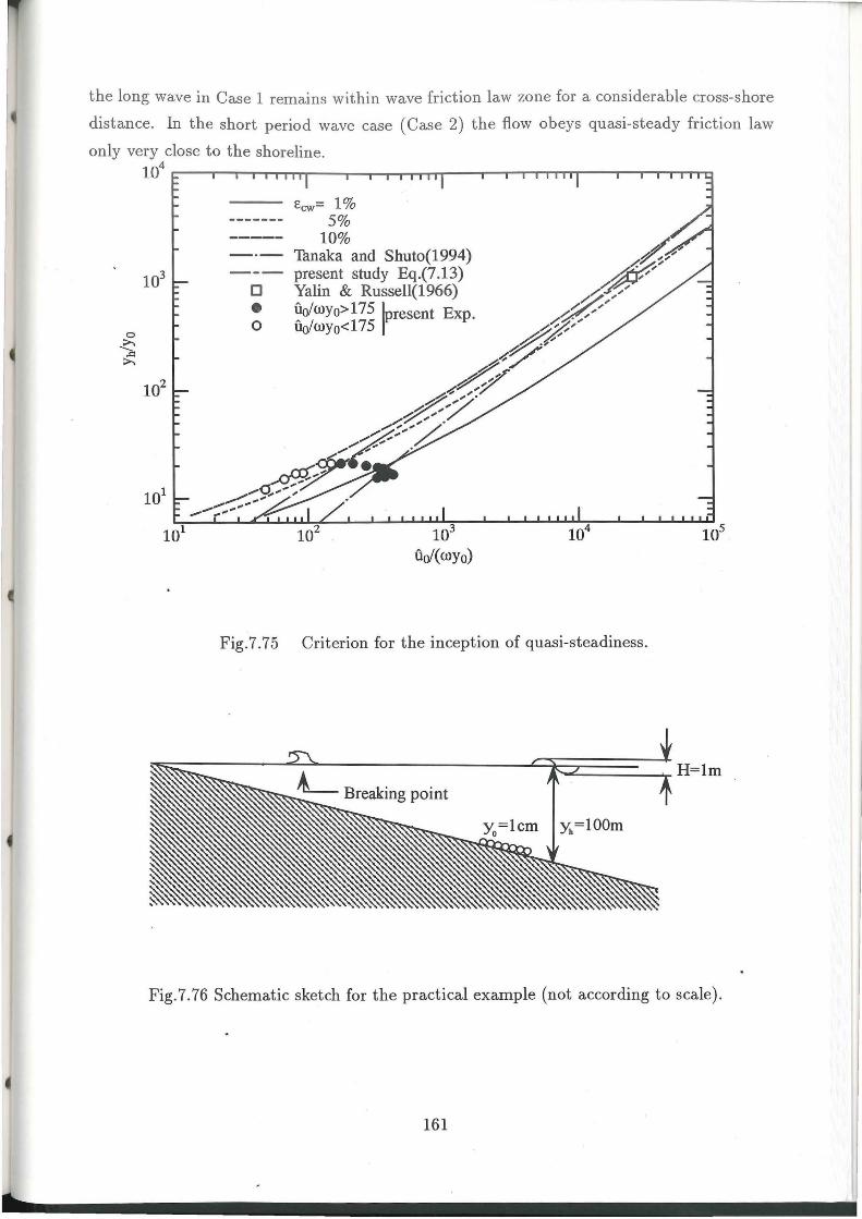
the long wave in Case 1 remains within wave friction law zone for a considerable cross-shore
distance. In the short period wave case (Case 2) the flow obeys quasi-steady friction law
only very close to the shoreline. 104 ~--.-~rrrnTr--~~~~~~~r-~-r~Tr--,--r~rn~
0
• 0
Ecw= 1% 5%
10% Tanaka and Shuto(1994) present study Eq.(7.13) Yalin & Russell(1966) fiolwyo> 175 lnresent Exp . fio/wyo<175 r
Fig.7.75 Criterion for the inception of quasi-steadiness.
Fig.7.76 Schematic sketch for the practical example (not according to scale).
161

-NVJ N-._
s .._ a.. -6 0 ~
2
1
5
2
10-2
5 I I I I I
0
"~ '~
T=lO min H=lm at Yh=lOOm slope= 1/100
" .. ,, •
---Steady friction law(Eq.7.4)
...... ..... •.... St.lB ... ...... l ........
-------Wave friction law(Eq.7.9)
1000 2000 3000 Cross-shore distance(m)
Fig.7.77 Variation of parameters in cross-shore direction for Case 1.
162

0.04
~ >. 0.02
2
1
5
,.-.. ('I
00 ('1-
g 2 a. 8
0 ~
10- 2
5
0
T=lO sec
slope= 1/100
wave
H=lm at Yh=lOOm
• theory(Tanaka and Shuto,1994)
__ ....;.· Steady friction law(Eq.7.4)
............. Wave friction law(Eq.7.9)
20 40 60 Cross-shore distance(m)
1
80 100
Fig. 7. 78 Variation of parameters in cross-shore direction for Case 2.
163

10°
5
-.. 8 '-" >.
10-1
5
-2
-2 0 u(m/sec)
St.lA
2 - 1 0 u(m/sec)
Fig.7.79 Velocity profiles at St.lA and St.lB for Case 1.
0 u(m/sec)
St.2A
2 -1 0 u(m/sec)
Fig.7.80 Velocity profiles at St .2A and St.2B for Case 2.
164
1
1

lease 1 (T=lO min.) !... .. ·· . ..
lease 2 (T=lO sec.)l
~( ... ·······.: . ...-- BP
.. ..
wave friction law zone
·· ... .. ·· ...
quasi-steady friction law zone
Fig. 7.81 Regime diagram for the range of applicability of steady and wave friction laws.
7.5 Conclusion
1. A detailed experimental study has been carried out to explore the properties of a
quasi-steady wave boundary layer on a rough bottom. Significant differences were
found between the ordinary and quasi-steady wave boundary layer in connection with
the velocity profile, turbulence intensity, momentum balance and friction factor.
2. It is inferred that only longer period of oscillation is not sufficient to produce . quasi
steady effects, but the real parameter is u0jwyh as shown in a theoretical study by
Tanaka and Shuto(1994).
3. The criterion for the inception of quasi-steadiness is modified to increase its range of
. applicability.
4. This modified criterion is then applied to a practical case to demonstrate its impor~ance
in the real situations.
165

8 SUMMARY OF CONCLUSIONS AND FUTURE
RECOMMENDATIONS
The present study was aimed at the exploration of unsteady boundary layers of practical
relevance by using two-equation turbulence model(k - t::) in addition to an extensive exper
imental program. As a result of the present study, although many interesting results have
bee~ obtained regarding transition in sinusoidal oscillatory boundary layers, quasi-steady be
havior for friction in oscillatory boundary layers and asymmetric oscillatory boundary layers ,
however, new questions have arisen to carry-out future research regarding these topics.
The conclusions of the present study and recommendations for future research may be
broadly classified into two groups, i.e. experimental and numerical aspects.
8.1 Experimental Aspects
8.1.1 Sinusoidal oscillatory boundary layer transition
The present study on transition from laminar to turbulence m an oscillatory boundary
layer of sinusoidal type revealed some of the interesting features regarding the cross-stream
phase difference profile. In one of the previous studies though such type . of behavior was
anticipated (see Cousteix et al. , 1981), however detailed measurement was not carried out .
The present study may therefore be considered as complementary to the experimental study
by Jensen(1989) who did not discuss the transition from this point of view in detail.
There is a lot more to investigate regarding the complex phenomenon of transition
especially with a view to test the existing turbulence models . In the present study only
streamwise fluctuating component of velocity was measured whereas Jensen(1989) measured
two components. But in order to test k- E and other higher turbulence models , the three
components must be measured in order to compute turbulence kinetic energy.
8.1.2 Boundary layer under wave-current combined motion
During the course of present study, the experiments were performed under wave-current
combined motion and the velocity was measured by LDV. It was observed that the bound
ary layer remains unaltered by the imposed current, whereas the current profile is deformed.
Moreover, the turbulence intensity is increased in whole cross stream dimension by the
interaction of current and oscillatory components. In order to further understand the phe
nomenon of transition from laminar to turbulent under wave-current combined motion , an
extensive experimental program may be recommended. In addition to the velocity measure
ment, direct meaaurement of shear stress would be of great value. As a guideline to chalk
out the experimental plan, the regime diagram for wave-current combined motion proposed
by Tanaka and Thu(1994) may be employed.
166

8.1.3 Asymmetric oscillatory boundary layers
Another important experimental study may be related to the asymmetric oscillatory bound
ary layers. In the present study a few experiments were performed in this regard. It was
noted that the boundary layer thickness under trough is greater than that under crest at
high degree of asymmetry. The wall shear stress showed a transitional behavior similar to
that observed in sinusoidal oscillatory boundary layers. However, the direct measurement
of wall shear stress would elaborate the transitional properties. The detailed experiments
covering the transitional _and fully turbulent regimes may be very important from practical
point of view. Then it may be possible to test various analytical and numerical models and
semi-empirical methods regarding asymmetric oscillatory boundary layers.
Moreover, the piston movement system used in the present study may produce asym
metry with respect to time as well, thus producing an oscillation similar to the waves in
surf zone as shown by Tanaka et al.(1996). The experiments under such type of oscillatory
boundary layers would be of great practical value.
8.1.4 Quasi-steady oscillatory boundary layers
The transformation of an ordinary oscillatory boundary layer to a quasi-steady one is of
broad practi~al interest to coastal engineers. That is why a number of experiments were
performed as a part of the present study. It was observed that the parameter u0 / (wyh)
is the one to distinguish between ordinary and quasi-steady oscillatory boundary layers as
mentioned by Tanaka and Shuto(1994). As this parameter increases, so does the boundary
layer thickness until it becomes equal to Yh· Under this condition the cross-stream velocity
profile at every instant resembles that under steady flow.
Due to the restricted length of oscillating tunnel, it was possible to produce quasi-steady
effects only over very high roughness, i.e. small value of Yh/Yo· Therefore, for the future
studies in this regard, it is recommended that the experiments may be performed under
smaller roughness than the present one also, in order to observe the transformation from
ordinary to quasi-steady boundary layer under higher values of Yh / Yo ·
8.2 Numerical Aspects
8.2.1 k- E model
The predictive capabilities of low Reynolds number k - E model were explored in detail in
the present study in order to analyze oscillatory boundary layers. It has been inferred that
the performance of this model for these boundary layers is promising. As far as sinusoidal
boundary layers are concerned, the performance of low Reynolds number k - E model is ex-
167

cellent as has been demonstrated in Chapter 3 and 4. Although some of the modern models
are found to predict the turbulence energy and wall shear stress in a better manner than the
original version by Jones and Launder(1972). However, this model is very attractive from
practical point of view due to its less rigid initial condition requirement and more computa
tional economy than the models with non-zero wall boundary condit ion oft:. Moreover, this
model has been found to be superior among all the tested versions by virtue of its excellent
pe.rformance in predicting transitional properties.
The incorrect limiting behavior of JL model is although, of minor concern for field
applications , however; in order to capture fine details of the boundary layer structure near
the wall, the appropriate modification is mandatory.
The JL model was applied to the asymmetric oscillatory boundary layer also. It showed
good performance in predicting mean velocity during acceleration phase, but during deceler
ation its prediction was not up to the mark. The reason for that remains unclear, however,
this discrepancy may be attributed to the fact that this model can not perform well under
adverse pressure gradients as shown by other researchers. As mentioned before(see Chapter
6), the modeled equation of transport for kinetic energy dissipation rate is generally held
responsible for this shortcoming. Therefore, the procurement of a detailed data source to
propose the modifications in this equation to account for adverse pressure gradient effects is
essential..
A modified k- t: model with correct limiting behavior near the wall and appropriate
dissipation rate equation is required for an effective use of this model in field applications of
coastal engineering.
8.2.2 Higher order models
Although present day higher order models need lot of refinement in order to predict various
flow phenomena and these models are not practically as attractive as k- t: model, however,
the testing of these models may be carried out by using the present experimental data of
a challenging case like asymmetric oscillatory boundary layers. The results of what might
provide some guidelines to improve the predictive abilities of these models as well.
168

REFERENCES
Akhavan, R., Kamm, R. D. & Shapiro, A. H. 1991 An investigation of transition to turbu
lence in bounded oscillatory Stokes flows, Part 1. Experiments. J. Fluid Mech . 225 ,
395-422.
Armanini, A. & Ruol, P. 1988 Non-uniform suspended sediments under waves . In Proc .
. 21st Int. Conf. Coastal Eng., 1129-1139.
Asano, T. & Iwagaki, Y. 1984 Bottom turbulent boundary layer in wave-current co-existing
systems. In Proc. 19th Int. Conf. Coastal Eng ., 2397-2413.
Asano, T. & Iwagaki , Y. 1986 Nonlinear effects on velocity fields in turbulent wave boundary
layers. Coastal Eng. Japan 29 , 51-63.
Asano, T ., Godo, H. & Iwagaki , Y. 1988 Application of low-Reynolds number turbulence
model to oscillatory bottom boundary layers. Coastal Eng. Japan 30 No.2 , 1-9.
Aukrust , T. & Brevik, I. 1985 Turbulent viscosity in rough oscillatory flow. J. Waterway
Port Coastal Ocean Eng. 111 No.3, 525-541.
Aydin, I. & Shu to, N. 1988 An application of the k-c model to oscillatory boundary layers.
Coastal Eng. Japan 30, No.2, 11-24.
Bakker, W. T . 1974 Sand concentration in oscillatory flow. In Proc. 14th Int . Conf. Coastal
Eng. , 1129-1148. ::
Bijker, E. W. 1966 The increase of bed shear in a current due to wave motion. In Proc.
10th Int. Conf. Coastal Eng., 746-765.
Blondeaux, P. 1987 Turbulent boundary Layer at the bottom of gravity waves. J. Hyd.
Res. 25, No.4, 44 7-464.
Blondeaux, P. & Colombini , M. 1985 Pulsatile turbulent pipe flow. In Proc. 5th Symp.
Turb. Shear Flows, 16.15-16.21.
Brevik, I. 1981 Oscillatory rough turbulent boundary layers. J. Waterway Port Coastal
Ocean Eng. 103, 175-188.
Carr, L. W. 1981 A review of unsteady turbulent boundary-layer experiments. In IUTAM
Symp., 1-34.
Chien, K.-Y. 1982. Predictions of channel and boundary-layer flows with a low-Reyrrolds
number turbulence model. AIAA J. 20 No.1, 33-38.
Christoffersen, J. B. 1982 Current Depth Refraction of Dissipative Waves, Series Paper
No.30, ISVA, Technical Univ. of Denmark.
169

Christoffersen, J. B. & Jonsson , I. G. 1985 Bed friction and dissipation in a combined
current and wave motion. Ocean Eng. 12 No.5, 387-423.
Cousteix, J ., Desopper, A. & Houdeville, R. 1976 Recherches sur les couches limits tur
bulentes instationaires. (Research on unsteady turbulent boundary layers). ON
ERA/DERAT, TP 1976-147, Toulouse, France (In French).
Cousteix, J. , Desopper, A. & Houdeville, R. 1979 Structure and development of a turbulent
· boundary layer in an oscillatory external flow. Turbulent Shear Flows 1, 154-171.
Cousteix, J . & Houdeville, R. 1985 Turbulence and skin friction evolutions in an oscillating
boundary layer. In Proc. 5th Symp. Turb. Shear Flows, 18.7-18.12.
Cousteix, J., Javelle, J . & Houdeville, R. 1981 Influence of Strouhal number on the structure
of flat plate turbulent boundary layer. Turbulent Shear Flows 3, 46-59.
Eckmann, D. M. & Grotberg, J. B. 1991 Experiments on transition to turbulence in oscil
latory pipe flow. J. Fluid Mech. 222, 329-350.
Freds(<1e, J. 1984 Turbulent boundary layer in wave-current motion. J. Hyd. Eng. 110
No.8, 1103-1120.
Freds(<1e, J. & Deigaard, R. 1992 Mechanics of Coastal Sediment Transport World Scientific,
Sing~pore.
Freds(<1e, J., Sumer, B. M. , Laursen, T . S. & Pedersen, C. 1993 Experimental investigation
of wave boundary layer with a sudden change in roughness. J. Fluid Mech. 252,
117-145.
Goda, Y. 1975 Deformation of irregular waves due to depth-controlled wave breaking. Rep.
Port Harbour Res. Inst. 14 No.3, 59-106.
Grant, W.D. & Madsen, O.S. 1979 Combined wave and current interaction with a rough
bottom. J. Geophysical Res. 84 No.C4, 1797-1808.
Hagatun, K. & Eidsvik, K. J. 1986 Oscillating turbulent boundary layer with suspended
sediments. J. Geophysical Res. 91, C11, 13045-13055.
Ha Minh H. , Viegas, J. R., Rubesin, M. W., Vandrome, D. D. & Spalart, P. R. 1989.
Physical analysis and second order modelling of an unsteady turbulent flow: The
oscillating boundary layer on a flat plate. In Proc. 7th Symp. Turb. Shear Flows,
paper 11-5.
Hanjalic, K., Jakirlic, S. & Hadzic, I. 1995. Computation of oscillating turbulent flows at
transitional ~eynolds numbers. In Turb. Shear Flows 9, 323-342.
Hanjalic, K. & Launder, B. E. 1980. Sensitizing the dissipation equation to irrotational
strains. J. Fluids Eng., Trans. ASME, 102, 34-40.
170

Hanjalic, K. & Stosic, N. 1983. Hysteresis of turbulent stresses in wall flows subjected to
periodic disturbances. In Proc. 4th Symp. Turb. Shear Flows, 8.12-8.17.
Hino, M., Sawamoto, M. & Takasu, S. 1976 Experiments on transition to turbulence in an
oscillatory pipe flow. J. Fluid Mech. 75, 193-207.
Hino, M., Kashiwayanagi, M., Nakayama, A. & Hara, T. 1983 Experiments on the turbu
lence statistics and the structure of a reciprocating oscillatory flQw. J. Fluid Mech.
131, 363-400.
Huynh-Thanh, S. & Temperville, A. 1990 A numerical model of the rough turbulent bound
ary layer in combined wave and current. In Proc. 22nd Int. Conf. Coastal Eng.,
853-866.
Jacobs, S. J. 1984 Mass transport in a turbulent boundary layer under a progressive water
wave. J. Fluid Mech. 146, 303-312.
Jensen, B. L. 1989 Experimental Investigation of Turbulent Oscillatory Boundary Layers,
Series Paper No.45, ISVA, Technical Univ. of Denmark.
Johns, B. 1975 The form of velocity profile in a turbulent shear wave boundary layer. J.
Geophysical Res. 80 No.36, 5109-5112.
Johns, B. 1977 Residual flow and boundary shear stress in the turbulent bottom layer
beneath waves. J. Phys. Oceanography 7, 733-738.
Jones, W. P. & Launder, B. E. 1972 The prediction of laminarization with a two-equation
model of turbulence. Int. J. Heat Mass Transfer 15, 301-314.
Jonsson, I. G. 1963 Measurements in the turbulent wave boundary layers. In Proc. 10th
Gong. IAHR, 85-90.
Jonsson, I. G. 1966 Wave boundary layers and friction factors. In Proc. 1Oth Int. Conf.
Coastal Eng., 127-148.
Jonsson, I. G. 1978 A New Approach to Oscillatory Rough Turbulent Boundary Layers,
Series Paper No.l7, ISVA, Technical Univ. of Denmark.
Jonsson, I. G. & Carlsen, N. A. 1976 Experimental and theoretical investigations in an
oscillatory turbulent boundary layer. J. Hyd. Res. 14 No.1, 45-60.
Justesen, P. 1988 Turbulent Wave Boundary Layers, Series Paper No.43, ISVA, Technical
Univ. of Denmark.
Justesen, P. 1991 A note on turbulence calculations in the wave boundary layer. J. Hyd.
Res. 29, No.5, 699-711.
171

Justesen, P. & Spalart , P.R. 1990. Two equation turbulence modeling of oscillatory bound
ary layers, AIAA paper 90-0496.
Kajiura, K. 1964 On the Bottom friction in an oscillatory current. Bull. Earthquake Res.
Inst. 42, 14 7-174.
Kajiura, K. 1968 A model of the bottom boundary layer in water waves. Bull. Earthquake
Res. Inst. 46, 75-123.
Kamphuis, J. W. 1975 Friction factor under oscillatory waves. J. Waterways Harbors
Coastal Eng. 101, No. WW2, 135-144.
Kebede, W., Launder, B. E. & Younis, B. A. 1985 Large-amplitude periodic pipe flow: A
second moment closure study. In Proc. 5th Conf. Turb. Shear Flows, 16.23-16.29.
Kemp, P. H. & Simons, R. R. 1982 The interaction between waves and a turbulent current:
waves propagating with the current. J. Fluid Mech. 116, 227-250.
Kemp, P. H. & Simons, R. R. 1983 The interaction of waves and a turbulent current: waves
propagating against the current. J. Fluid Mech. 130, 73-89.
Kwon, 0 . K., Pletcher, R. H. & Delaney, R. A. 1988 Solution procedure for unsteady
two-dimensional boundary layers. J . Fluids Eng. ASME 110, 69-75.
Lam, C:K. G. & Bremhorst, K. J. 1981 A modified form of the k- t: model for predicting
wall turbulence. J. Fluids Eng. ASME 103, 456-460.
Larsen, M. 1995 Closed-form solution for turbulent wave boundary layers . . In Proc. Japanese
Conf. Coastal Eng. 42, 26-30, (In Japanese).
Launder, B. E. & Spalding, D. B. 1974 The numerical computation of turbulent flows.
Comp. Methods App. Mech. Eng. 3, 269-289.
Lundgren, H. 1972 Turbulent currents in the presence of waves. In Proc. 13th Int. Conf.
Coastal Eng., 623-634.
Markatos, N. C. 1986 The mathematical modelling of turbulent flows. App. Math. Mod.
10, 190-220.
Mizushina, T. , Maruyama, T. & Shiozaki, Y. 1973 Pulsating turbulent flow in a tube. J.
Chem. Eng. Japan 6 No.6, 487-494.
Mizushina, T. , Maruyama, T. & Hirasawa, H. 1975 Structure of the turbulence in pulsating
pipe flow. J. Chem. Eng. Japan 8 No.3, 210-216.
Myong, H. K. &z: Kasagi, N. 1990 A new approach to the improvement of k - t: turbulence
model for wall-bounded shear flows. JSME Int. J., Series II 33 No. 1, 63-72.
172
Myrhaug, D. 1982 On a theoretical model of rough turbulent wave boundary layers. Ocean
Eng. 9 No.6, 547-565.
Myrhaug, D. 1984 A note on a theoretical model of oscillatory smooth turbulent boundary
layers. Ocean Eng. 11 No.3, 315-320.
Myrhaug, D. & Slaattelid, O.H. 1989 Combined wave and current boundary layer model
for fixed rough seabed. Ocean Eng. 16 No.2, 119-142.
Nadaoka, N., Yagi , H., Nihei, Y. & Nomoto, K. 1994 Characteristics ofturbulence structure
in asymmetrical oscillatory flow. In Proc. Japanese Conf. Coastal Eng. 41 , 141-145,
(In Japanese).
Nadaoka, N., Nihei, Y., Yagi, H. & Nomoto, K. 1996 Characteristics ofturbulence structure
in asymmetrical oscillatory flow . In Proc. Japanese Conf. Coastal Eng. 43, 441-445,
(In Japanese).
Nagano, Y. & Tagawa, M. 1990 J. An improved k- t model for boundary layer flows. J.
Fluids Eng. ASME 112, 33-39.
Nallasamy, M. 1987 Turbulence models and their applications to the prediction of internal
flows: A review. Computers and Fluids 15 No.2, 151-194.
Nezu, L 1977 Turbulent structure in open channel flows. Ph. D. Dissertation, Kyoto Univ.,
Japan, (In Japanese).
Patel, V. C., Rodi, W. & Scheuerer, G. 1985 Turbulence models for near-wall and low
Reynolds number flows: A review. AIAA J. 23 No.9, 1308-1319.
Ribberink, J. S. & Al-Salem, A. 1995 Sheet flow and suspension of sand in oscillatory
boundary layers. Coastal Eng. 25, 205-225.
Rodi, W. 1984 Turbulence Models and Their Application in Hydraulics-A State of the Art
Review, IAHR, The Netherlands.
Rodi, W. & Scheuerer, G. 1986 Scrutinizing the k - t turbulence model under adverse
pressure gradient conditions. J. Fluids Eng., Trans. ASME 108, 174-179.
Sarpkaya, T. 1993 Coherent structures in oscillatory boundary layers. J. Fluid Mech. 253,
105-140.
Sana, A. 1992 Application of a Turbulence Model to an Oscillatory Boundary Layer, M.
Eng. Thesis , No.WA-92-1, Asian Institute of Technology, Bangkok, Thailand.
Sana, A. & Tanaka, H. 1995 A full-range equation for wave boundary layer thickness . In
Advances· in Hydro-Science and Eng. 2, 1487-1494.
173

Sato, S., Uehara, H. & Watanabe, A. 1986 Numerical simulation of the oscillatory boundary
layer flow over ripples by a k - E turbulence model. Coastal Eng. Japan 29, 65-78.
Sawamoto, M. & Hino, M. 1977 Frictional resistance law for an oscillatory pipe flow with
smooth boundaries. Proc. of JSCE 258, 45-53 (in Japanese).
Sawamoto, M. & Sato, E. 1991 The structure of oscillatory turbulent boundary layer over
rough bed. Coastal Eng. Japan 34 No.1, 1-14.
Sheng, Y. P. 1982 Hydraulic applications of a second-order closure model of turbulent
transport. In Applying Research to Hydraulic Practice, 106-119.
Sheng, Y. P. 1984 A turbulent transport model of coastal processes. In Proc. 19th Int.
Conf. Coastal Eng., 2380-2396.
Shima, N. 1993. Prediction of turbulent boundary layers with a second moment closure:
part 1. J . of Fluids Eng. ASME 115, 56-69.
Sleath, J.F.A. 1987 Turbulent oscillatory flow over rough beds. J. Fluid Mech. 182, 369-
409.
Sleath, J. F. A. 1990 Seabed boundary layers. In The Sea 9B, 693-727.
Smith, J. D. 1977 Modeling of sediment transport on continental shelves. In The Sea 6,
539-5!78.
So, R. M. C. , 1ai, Y. G. , Zhang, H. S. & Hwang, B. C. 1991 Second-order near-wall
turbulence closures: A review. AIAA ]. 29 No.ll, 1819-1835.
Soulsby, R. 1., Hamm, 1., Klopman, G., Myrhaug, D., Simons, R. R. & Thomas, G. P.
1993 Wave-current interaction within and outside the bottom boundary layer. Coastal
Eng. 21, 41-69.
Spalart, P.R. & Baldwin, B. S. 1989 Direct simulation of a turbulent oscillating boundary
layer. In Turbulent Shear Flows 6, 417-440.
Speziale, C. G. 1991 Analytical methods for the development of Reynlds stress closures in
turbulence. In Annual. Rev. Fluid Mech. 23, 107-157.
Speziale, C. G., Abid, R. & Anderson, E. C. 1992 Critical evaluation of two-equation models
for near-wall turbulence. AIAA J. 30 No. 2, 324-331.
Supharatid ,S., Tanaka, H., & Shuto ,N. 1992 Interaction of Nonlinear Wave and Current.
In Proc. 23rd Int. Conf. Coastal Eng., 672-683.
Takahashi, T. Imamura, F. & Shuto, N. 1993 Numerical simulation of topography change
due to tsunamis. In Proc. of IUGG/IOC Int . Tsunami Symp., Japan, 243-255.
174

Tanaka, H. 1986 Turbulence structure and bed friction under waves and current interacted
motion. In Proc. 3rd Int. Symp. River Sed., 334-343.
Tanaka, H. 1992 An explicit expression of friction coefficient for wave-current coexistent
motion. Coastal Eng. Japan, 35 No.1, 83-91.
Tanaka, H. , Chian, C. S. & Shuto , N. 1983 Experiments on an oscillatory flow accompanied
with a unidirectional motion. Coastal Eng. Japan 26, 19-37.
Tanaka, H. & Sana, A. 1994 Numerical study on transition to turbulence in a wave boundary
layer. In Sediment Transport M echanism in Coastal Environments and Rivers, 14-25.
Tanaka, H., & Shuto, N. 1981 Friction Coefficient for a Wave-Current Coexistent System.
Coastal Eng. Japan 24, 105-128.
Tanaka, H., & Shuto, N. 1994 Quasi-steady property of bottom friction in a wave boundary
layer. In Int . Symp. Waves-Phys. Num. Mod., 1570-1579.
Tanaka, H. & Thu, A. 1994 Full range equation of friction coefficient and phase difference
in a wave-current boundary layer. Coastal Eng. 22, 237-254.
Tanaka, H., Sumer, B. M. & Freds¢e, J . 1996 Theoretical and experimental investigations
on laminar boundary layer under cnoidal wave motion. J. Hyd. Coastal Environment
Eng . ( JSCE}, (in preparation)(in Japanese).
Tanaka, H., Yamaji, H., Sana, A. & Shuto, N. 1996 A new generation method of asymmetric
oscillatory flow. J. Hyd. Coastal Environment Eng. (JSCE), (accepted)(in Japanese) .
Tardu, S. F., Binder, G. & Blackwelder, R. F. 1994 Turbulent channel flow with large
amplitude velocity oscillations. J. Fluid Mech. 267, 109-151.
Taulbee, D. B. 1989 Engineering turbulence models. In Advances in Turbulence , 75-125.
Thomas, G. P. 1981 Wave-current interactions: an experimental and numerical study. Part
1. Linear waves. J. Fluid Mech. 110, 457-474.
Trowbridge, J. H., Kanetkar, C. N. & Wu, N. T. 1986 Numerical simulation of turbulent
wave boundary layers. In Proc. 20th1nt. Conf. Coastal Eng., 1623-1637.
Trowbridge, J. H. & Madsen, 0. S. 1984 Turbulent wave boundary layers. J. Geophysical
Res. 89 No. C5, 7989-7997.
Tsuchiya, Y. & Banno, M. 1988 The criterion of ripple formation by wave action. In Proc.
20th Int. Conf. Coastal Eng., 1868-1881.
Tu, S. W., &_ Ramaprian, B. R. 1983 Fully developed periodic turbulent pipe flow. Part
1. Main experimental results and comparison with predictions. J. Fluid Mech . 137,
31-58.
175

Van Kestern, W. G. M. & Bakker, W. T. 1984 Near bottom velocities in waves with a
current: analytical and numerical computations. In Proc. 19th Int. Conf. Coastal
Eng., 1161-1177.
Van Rijn, L. C., Nieuwjaar, W. C., Kaay, T. V. D., Nap, E. & Kampem, A. V. 1993
Transport of fine sands by currents and waves. J. Waterway, Port, Coastal and Ocean
Eng. 119 No.2 , 123-143.
Visser, P. J. 1986 Wave basin experiments on bottom friction due to current and waves. In
Proc. 20th Int. Conf. Coastal Eng., 807-821.
Vonvisessomjai, S. 1984 Oscillatory boundary layer and eddy viscosity. J. Hyd. Eng. 110
No.4, 387-404.
Vonvisessomjai, S. 1985 Regime of oscillatory flow. J. Waterway Port Coastal Ocean Eng.
111 No.1, 96-110.
Yalin, M. S. & Russell , R. C. H. 1966 Shear stresses due to long waves. J. Hyd. Res. 4,
No.2 , 55-98.
You, Z. J., Wilkinson, D. L. & Nielsen, P. 1991 Velocity distributions of waves and currents
in the combined flow. Coastal Eng. 15, 525-543.
You, Z. J. , Wilkinson, D. L. & Nielsen, P. 1992 Velocity distribution in turbulent oscillatory
boundary layer. Coastal Eng. 18, 21-38.
Young, J. S. L. & Sleath, J. F. A. 1989 Initial motion in combined wave and current flows.
In Proc. 21st Int. Conf. Coastal Eng., 1140-1151.
176

APPENDIX I
Finite Difference Scheme
In the present study, an exponentially increasing grid spacing was used in order to get better
accuracy near the wall. The definition sketch for the finite difference scheme is shown in
Fig.I.l.
e location of u,k,E
X location of Vt
Wall
L\yi-1
------- Axis of symmetry
i+l
1
i-1
Fig.I.l Finite difference scheme.
The dimensionless governing equations, i.e. equation of motion (Eq.3.21 ), equation
for transport of kinetic energy (Eq.3.22) and equation for transport of turbulence energy
dissipation rate (Eq.3.23) may be expressed in the following form by using a Crank Nicolson
type implicit scheme (avoiding the superscipt '*');
Equation of motion:
Ui,j+l - Ui,j
!:l.t
Equation of transport for turbulence kinetic energy:
I-1
(I.l)

k· "+1- k·. t,) t,)
!:1t
Equation of transport for turbulence kinetic energy dissipation rate:
Ei,j+l - Ei,j
!:1t ~ [ { :y ( ~~ + ;. v,) :; } ; + { ~ ( :e + :. v,) :; } J +~SC,C" [ {f.k (::) l + {f"k (::) 1J -~SC2 [{h ~ L + {h f L+l] + ~S(Ej + Ej+I)
By considering the Fig.l.l, for any variable '1/J;
where, '1/J = u, k, E, the first derivative of any quantity '1/J may be expressed as;
(1.2)
(1.3)
a'l/J = ( '1/Ji+l - 'l/J;)I:1Yi-1 ( '1/Ji+l _ '1/J;) _ ( '1/J; - 'l/Ji-1)!:1y; ( '1/Ji _ '1/Ji-l) (I.s) ay !:1y;(l:1yi + !:1yi-1) !:1Yi-1(!:1y; + !:1Yi-l)
By using the above finite difference scheme all the three governing equations may be
expressed in a general form as follows;
(1.6)
The coefficients A;1 , A;2 , A;3 and A;4 form the elements of a tridiagonal matrix which
may be solved by Gauss elimination method.
1-2
-


