Experimental Large-Scale Jet Flames’ Geometrical Features Extraction forRisk Management Using Infrared Images and Deep Learning Segmentation

Methods

Carmina Perez-Guerreroa, Adriana Palaciosb,∗, Gilberto Ochoa-Ruiza,∗, Christian Matac, Joaquim Casalc,Miguel Gonzalez-Mendozaa, Luis Eduardo Falcon-Moralesa

aTecnologico de Monterrey, School of Engineering and Sciences, Jalisco, 45138, Mexico.bUniversidad de las Americas Puebla, Department of Chemical, Food and Environmental Engineering, Puebla, 72810,

Mexico.cUniversitat Politecnica de Catalunya. EEBE, Eduard Maristany 16, 08019 Barcelona. Catalonia, Spain.

Abstract

Jet fires are relatively small and have the least severe effects among the diverse fire accidents that can occurin industrial plants; however, they are usually involved in a process known as the domino effect, that leadsto more severe events, such as explosions or the initiation of another fire, making the analysis of such firesan important part of risk analysis. This research work explores the application of deep learning models inan alternative approach that uses the semantic segmentation of jet fires flames to extract the flame’s maingeometrical attributes, relevant for fire risk assessments. A comparison is made between traditional imageprocessing methods and some state-of-the-art deep learning models. It is found that the best approach is adeep learning architecture known as UNet, along with its two improvements, Attention UNet and UNet++.The models are then used to segment a group of vertical jet flames of varying pipe outlet diameters toextract their main geometrical characteristics. Attention UNet obtained the best general performance in theapproximation of both height and area of the flames, while also showing a statistically significant differencebetween it and UNet++. UNet obtained the best overall performance for the approximation of the lift-offdistances; however, there is not enough data to prove a statistically significant difference between AttentionUNet and UNet++. The only instance where UNet++ outperformed the other models, was while obtainingthe lift-off distances of the jet flames with 0.01275 m pipe outlet diameter. In general, the explored modelsshow good agreement between the experimental and predicted values for relatively large turbulent propanejet flames, released in sonic and subsonic regimes; thus, making these radiation zones segmentation models,a suitable approach for different jet flame risk management scenarios.

Keywords: jet fire; risk management; deep learning; semantic segmentation; flame height; lift-off.

1. Introduction

Certain industrial activities, that take place in process plants or during the storage and transportation ofhazardous materials, can face severe accidents. The effects of these major accidents can have consequencesbeyond the activity’s boundary and affect external factors such as human health, environmental impact, orproperty damage. The accuracy in the evaluation of the effects and consequences that derive from theseaccidents presents a great area of opportunity that can be tackled by the improvement of the knowledgeof the main features of the most common major accidents. A complete understanding of these features isessential to avoid them, or in the worst-case scenario, to reduce and limit their consequences and severity.

∗Corresponding author: adriana.palacios@udlap.mx; gilberto.ochoa@tec.mx

Preprint submitted to Journal of Loss Prevention in the Process Industries January 21, 2022

arX

iv:2

201.

0793

1v1

[cs

.CV

] 2

0 Ja

n 20

22

Some accidents are well known and have been thoroughly explored nowadays, however, some other accidentspresent various gaps in knowledge that could be investigated.

Jet fires are one kind of fire accident that have been repeatedly found to initiate domino effects, whoseconsequences could lead to catastrophic events in the process industries. Gomez-Mares, Zarate, and Casal[1] performed a historical survey based on over 84 cases obtained from four European accident databases.They reported that one in two jet fire events caused a domino effect, originating at least another fire accidentwith severe effects; explosions happened in 56% of the cases, a vapor cloud was generated in 26% of thecases, and other types of fires occurred in 27% of the cases; these percentages do not add up to 100%, giventhat more than one of these events can occur at the same time. It was also found that propane was themost common fuel involved since jet fires are usually originated by the loss of containment and ignition offlammable gas, vapor, or spray. The flammable elements may be released through a hole, a broken pipe, aflange, or during process flares.

Jet fires tend to occur in rather compact spaces and the probability of flame impingement on anotherequipment from the associated domino effect is rather high. Therefore, even though jet fires tend to beconfined to relatively shorter distances compared to other fire accidents, such as pool fires, flash fires, orfireballs, they have some specific features that can significantly increase the hazards associated with them.These features make them very important from a risk analysis point of view, which leads to the significanceof their proper characterization. Several authors have investigated the main geometrical features of jetflames. Some of these studies have been focused on the jet flame height ([2], [3], [4]) with recently proposedequations to predict jet flame height including several fuels and orientations [3]. The jet flame shape hasalso been predicted through several models ([5], [6], [7]), as well as the non-ignition zones ([3], [8]).

The most common jet fire consequence analyses rely mostly on empirical models that use a simplifiedflame geometry and fixed emissive power to determine the thermal radiation load on a target, thus, a popularapproach to evaluate both jet fire geometric features and radiation loads has been the use of ComputationalFluid Dynamics (CFD) [9]. However, Mashhadimoslem et al. [10] have recently found that CFD methodsrequire more computational time and have a higher cost impact than neural networks; less computation timeand higher accuracy are the hallmarks of neural networks for predicting processes, as well as their ability towork on more realistic data.

In the present work, the benefits of neural networks, from the field of Deep Learning, are assessed asa tool to develop an alternative approach that uses image segmentation for the approximation of jet flameheight, area, and non-ignition flame zone. These are relevant geometric features used in jet fire risk analysis,more specifically, to control the likelihood of direct flame impingement and to determine the distributionand intensity of radiant heat that is emitted from the flame to the surrounding equipment. Furthermore,the explored image segmentation approach can be used to optimize the parameters of other radiation andturbulence models, making the characterization of such geometrical and radiation factors, critical for theprocess safety field. In the present work, experimental data on large-scale jet flames, released in bothsonic and subsonic conditions, have been used along with recent developments in the image processing andcomputer vision fields, namely, recent algorithmic strides in the form of deep learning methods, to producehighly accurate segmentation masks used in image analysis tasks that characterize jet fires.

Deep learning algorithms, and more specifically, Convolutional Neural Networks (CNNs), are amongthe most extensively used and increasingly influential types of machine learning algorithms for computervision tasks and data-driven models. Convolutional networks have shown outstanding capabilities in manycomplex endeavors, such as image recognition, object detection, and semantic and instance segmentation[11]. Advancements on these techniques have been proliferating, and with cutting-edge research beingpublished constantly, better and more robust algorithms are emerging faster than ever.

Among the tasks where convolutional networks excel, instance and semantic segmentation have seena recent surge in technical progress. It extends and combines two of the most popular computer visiontasks: object detection and semantic segmentation. Its applications range from autonomous vehicles [12]to robotics [13] and surveillance systems [14], to name a few. Instance segmentation aims to assign classlabels and pixel-wise instance masks to identify a varying number of instances presented in each image orvideo frame [15]. Figure 1 illustrates the main differences between object classification, object detection, andsemantic segmentation, along with an example of the main geometrical characteristics that are extracted

2

from the segmentation. Object classification tries to assign a certain category to a full image, object detectionfocuses on locating and classifying an object with high precision, and semantic segmentation is interestedin finding the pixels of the image that correspond to certain elements, which in the case of this research, isthe boundaries of the jet fires.

(a) (b)

(c) (d)

Figure 1: Different computer vision tasks performed on a vertical jet flame of propane. Figure (a) is an example of objectclassification denoting the presence of the flame in the image. Figure (b) is an example of generic object detection using abounding box for the localization of the flame. Figure (c) is an example of semantic segmentation, signalling the name ofeach segment within the flame. Figure (d) is an example of the main geometrical characteristics that are extracted from thesegmentation.

Segmentation is a pre-processing stage from which other related problems can be solved. It can be used asan attention mechanism by focusing only on relevant parts of the images that can be further analyzed, suchas faces for bio-metric studies [16] or in the medical image analysis domain for image-guided interventions,radiotherapy, or improved radiological diagnostics [17]. Segmentation is useful for fine-grained tasks where abounding box around the objects is too coarse for a solution, especially when the scene is cluttered or whenthe precise entity boundaries are important [18]. Segmentation can also be used to change the pixels of animage into higher-level representations that are more meaningful, obtaining segments that represent objecttextures, locations, or shapes, which is important, for example, in the automatic interpretation of remotesensing images [19].

This paper uses the information obtained from exploratory research on different semantic segmentation

3

approaches, and a selection process of evaluation metrics, to single out the best method for the segmentationof fire ration zones. The selected model is trained on horizontal jet fires and then used to perform imagesegmentation on vertical jet fires. As a practical application of this approach, the segmented images areused to extract the flame’s geometrical information, and the results are then validated through previouscharacterization experiments.

Obtaining a model that can use the infrared features of the flame to extract its geometrical informationis a promising first step for the development of a reliable risk management system that could be usedfor general fire incidents. The segmentation experiments presented in this work could later be used tocharacterize the different radiation zones to improve the prediction of thermal radiation load on a target,going beyond defining just the main jet fire geometric features, which is the current focus of this research.Therefore, the work described in this manuscript is a contribution to the knowledge of the architecturesthat perform well for the segmentation of radiation zones within the fire, the most representative evaluationmethods to an expert’s criteria, and practical results obtained from the proposed approach, showing how itcan be used in the prediction of the main geometrical features of jet fires for accurate risk assessment andbetter prevention and control of jet fire accidents, which have been the origin of severe accidental scenarios,occurring worldwide in industrial establishments and during the transportation of hazardous materials.

The rest of this paper is organized as follows: Section 2 describes the previous work found in theliterature related to the problem. Section 3 contains a general description of the jet fire experimentalset-up and their characteristics, followed by a brief description of the data set used to train segmentationalgorithms and architectures. Section 4 describes the different segmentation approaches and introducesthe definition of the flame’s temperature boundaries and geometrical characteristics. This section alsoexplains the data pre-processing methods applied to the data set, the evaluation metrics used to compareand validate the models, and finally, the training process established for the training of the segmentationalgorithms. Section 5 presents the results of the comparison between the different segmentation models,along with the evaluation of the geometrical information extracted from the segmentation obtained throughthe best performing models. Finally, Section 6 summarizes the major findings of the presented research andoffers a discussion regarding the future work and areas of opportunity.

2. Literature Review

2.1. Jet Fire Thermal Radiation

Thermal radiation frequently plays a major role in the heat transfer process, therefore, fast and reliabletools to compute radiation emanating from flames are necessary for risk engineering applications. Somemodels are based on algebraic expressions and assume an idealized flame shape with uniform surface radiationemissive power, such as a cylindrical crone, proposed by Croce and Mudan [20], or a frustum of a coneproposed by Chamberlain [21].

Some other models, such as the line source emitter model, assume that the radiation source is representedas a line at the center of the flame. This model was used by Zhou and Jiang, who also proposed a profile ofemissive power per line length that can predict the radiant heat flux of jet flames with different flame shapesimulations [22].

Other models assume that the radiation is emitted by a single or multiple point sources distributedalong the flame surface. The Single Point Source model relies on the assumption that the radiation intensityemitted from the source is isotropic, but on the other hand, the Weighted Multi Point Source model considersthat the radiation emanates from N point sources distributed along the main axis of the flame. In Quezada,Pagot, Franca, and Pereira [23], they propose a new version of the inverse method for optimizing theWeighted Multi Point Source model parameters. The proposed new optimized weighting coefficients andthe new correlation for the radiative heat transfer rate showed improved results for predicting the radiativeheat transfer from the experiments.

A different approach to evaluate the consequences of the industrial hazards that jet fire accidents repre-sent, is through the use of Computational Fluid Dynamics (CFD). The models mentioned previously lackconsideration of the geometry of the system, which may make them unreliable when dealing with barriers

4

or equipment, therefore CFD represent an alternative solution for evaluating both the jet fire’s geometricfeatures and thermal radiation. For instance, Kashi and Bahoosh [24] explored different radiation and tur-bulence models along with CFD simulations to evaluate how firewalls or equipment around the flame canaffect the radiation distribution and temperature profile of the jet fire.

2.2. Jet Fire Geometrical Features

Fires are one of the most serious threats to the safety of both the equipment and the people who operatein process units. However, it is possible to identify the optimal space for the location of equipment andstructures, by evaluating the size and shape of the flames. Therefore, being able to predict the shape andproportions of a jet fire is extremely important from a risk management point of view [24]. Previous researchhas been done to characterize the main geometrical aspects of jet flames. For instance, Gautam [2] presentsa systematic study of the factors that affect the lift-off height, which is the distance between the burnerexit and the base of the lifted flame. It is found that the lift-off height varies linearly according to the exitvelocity, and it is independent of the burner diameter.

Palacios and Casal [5] analyzed the flame shape, length, and width of relatively large vertical jet firesat sonic and subsonic exit velocities. The flame boundary was defined at a temperature of 800 K, and theresults indicated that a cylindrical shape could accurately describe the shape, length, and diameter of theflame.

Zhang et al. [6] investigate the flame shape and volume of turbulent gaseous fuel jets with differentnozzle diameters. Baron’s model and Orloff’s image analysis method for shape prediction are compared.The results show that Baron’s method offers good predictions of the width and shape of the flame, with thewidth predictions being only slightly larger than the experimental results at the bottom and top sectionsof the flame. Based on the results, a mathematical model for flame volume estimation is deduced by theintegration of the Baron’s expression.

Bradley, Gaskell, Gu, and Palacios [3] introduce an extensive review and re-thinking of jet flame heightsand structure, including a proposal of dimensionless correlations for the atmospheric jet flames’ heights,lift-off distances, and mean flame surface densities. It was found that the same flow rate parameter couldbe used to correlate both heights and flame lift-off distances, and based on that, an equation was proposedto predict jet flame height including several fuels and orientations.

Guiberti, Boyette, and Roberts [4] explore the Delitcharsios’ model to obtain the flame height for subsonicjet flames at elevated pressure. The results show that the Delitcharsios’ model predicts well around 20% ofthe flame height in these cases, so a range of two empirical constants are suggested to improve the predictionsof the flame height equation.

Wang et al. [8] introduce a systematic experimental study on the lift-off behavior of jet flames impingingon cylindrical surfaces. The experiments are comprised of varying fuel exit velocity, internal diameters of thenozzle, and nozzle-to-surface spacing. An image visualization technique was used to reconstruct the imageframes of a camera and accurately calculate the flame lift-off distance. It was observed that the lift-offdistance depends on not only the exit velocity but also on the increase of nozzle diameter. It is also foundthat a dimensionless flow number expression for the lift-off distance provides the best fit.

Mashhadimoslem, Ghaemi, and Palacios [10] proposed an Artificial Neural Networks (ANN) approachthat uses the mass flow rates and the nozzle diameters to estimate the jet flame lengths and widths. The twomethods explored were a Multi-layer Perceptron method with Bayesian Regularization back-propagation anda Radial Based Function method with a Gaussian function. The two methods show negligible discrepanciesbetween them and can be used instead of Computational Fluid Dynamic methods, which require morecomputational time and have a higher cost impact than neural networks.

Wang et al. [7] present systematic experiments that show the effects of the nozzle exit velocity, diameter,and exit-plate spacing on the horizontal impingement of jet fires. The flame pattern and color are observedto evolve according to an increase in exit velocity and a decrease in exit-plate spacing. An Otsu method isused to calculate the flame intermittency probability. The probability contour of 50% is used to determinethe flame geometric features of interest to estimate the flame extension area. It is found that the temperatureprofile of the fire results in a big difference in the upward and downward directions along the vertical plate,so a uniform correlation, with the radius as the characteristic length scale, is proposed.

5

2.3. Automatic Fire and Smoke Monitoring

In the context of this research, segmentation is used to validate flame characterization experimentsby extracting geometrical information that can be used to reinforce principles of technological risks andindustrial safety. There has been previous work in the literature that have sought to apply automaticmethods to perform risk assessments in industrial security applications.

For instance, Janssen and Sepasian [25] presented an automatic flare-stack-monitoring system with flare-size tracking and automatic event signaling using a computer vision approach where the flare is separatedfrom the background by using temperature thresholding. To enhance the visualization of the temperatureprofile of the flare, false colors are added, representing the different temperature regions within the flare.Similarly, in Zhu et al. [26] an infrared image-based feedback control system was proposed to aid in fireextinguishing through automatic aiming and continuous fire tracking. To identify and localize the fire, animproved maximum entropy threshold segmentation method was employed. Threshold segmentation is thesimplest method of image segmentation and has a fast operation speed. However, it is not a very goodmethod to identify regions, but it represents a first step if combined with other segmentation techniques.[27].

Gu, Zhan, and Qiao [28] proposed a Computer Vision-based Monitor of Flare Soot, namely VMFS, whichis composed of three stages. First, they apply a broadly tuned color channel to localize the flame, then theyperform a saliency detection through K-means to determine the flame area, and finally use the center of it tosearch for a potential soot region. K-means clustering provides an efficient shape-based image segmentationapproach and has been used in other fire segmentation applications [29], [30]. Nonetheless, K-means is notvery effective when dealing with clusters of varying sizes and density since the centroids can be dragged byoutliers [31], and therefore the inherent dynamism of the fire may affect its results.

Ajith and Martınez-Ramon [30] proposed a computer vision-based fire and smoke segmentation system.Based on a feature extraction process, they test multiple clustering algorithms: K-Means clustering, GaussianMixture Model (GMM), Markov Random Fields (MRF), and Gaussian Markov Random Fields (GMRF).Even if MRF was found to be the model that distinguishes fire, smoke, and background in a more precisemanner, GMM was able to segment most of the fire regions but yielded a much lower accuracy for smokesegmentation. Bayesian methods for clustering such as these have no free parameters to adjust; however, anassumption on the class of the likelihood functions and the prior probabilities is needed for them to performwell.

Roberts and Spencer [32] proposed a method that introduces a new fitting term to the Chan-Vesealgorithm that allows the background to consist of multiple regions of inhomogeneity. This algorithmbelongs to the group of active contour models and is the most successful one among them when dealingwith infrared image segmentation [33]. The Chan-Vese model can achieve sub-pixel accuracy of objectboundaries and provides closed and smooth contours but it depends on several tuning parameters that haveto be manually selected and is used primarily for binary labels, so it needs to be applied multiple times orgeneralized to obtain multiple segments.

These different approaches perform well for data sets that they were developed on, however, it is necessaryto choose which features are important for each specific problem, so many aspects involve domain knowledgeand long processes of trial and error. Deep Learning architectures such as CNNs, in contrast, are able todiscover the underlying patterns of the images and automatically detect the most descriptive and salientfeatures with respect to the problem [34].

2.4. Deep Learning in Fire Scenarios

Convolutional Neural Networks have achieved state-of-the-art results in many computer vision tasks andan improvement on these models, that can recognize images at the pixel level and ensure robustness andaccuracy simultaneously, is found in Fully Convolutional Networks (FCNs) [35]. These architectures havethe ability to make predictions on arbitrarily sized inputs and have demonstrated outstanding results forsemantic image segmentation tasks; however, the propagation through several convolutional and poolinglayers affects the resolution of the output feature maps. Some advanced FCN-based architectures have beenproposed to address this flaw, some of the most notable are Deeplab, SegNet, and UNet.

6

DeepLabv3 [36] is composed of two steps, the encoding phase, where information about the object’spresence and location in an image is extracted, and the decoding phase, where the extracted information isthen used to reconstruct an output of appropriate dimensions. This architecture recovers detailed structuresthat may be lost due to spatial in-variance and has wider receptive fields; however, it shows low accuracyon small-scaled objects and has trouble capturing delicate boundaries of objects.

Segnet [37] consists of an encoder network, a corresponding decoder network, and a pixel-wise classifica-tion layer. It is designed to be efficient both in terms of memory and computational time during inferencebut its performance drops with a large number of classes and is sensitive to class imbalance.

The UNet [38] architecture consists of a contracting path that captures the context of images and asymmetric expanding path that enables precise localization of the segments. To predict the pixels in theborder region of the image, the missing context is extrapolated by mirroring the input image, which allowsfor precise localization of the regions of interest. This architecture, however, takes a significant amount oftime to train since the size of the network is comparable to the size of the features. It can also leave a highGPU memory footprint when dealing with large images. The Attention UNet [39] is an improved version ofUNet that uses attention gates to avoid excessive and redundant use of computational resources and featuremaps; however, these mechanisms add more weight parameters to the model, which further increases thetraining time.

UNet++ [40] is another improvement on the UNet architecture, which implements redesigned skip con-nections that aggregate features of different semantic scales, across an efficient ensemble of U-Net models ofvarying depths that partially share an encoder. This improvement overcomes the downsides of UNet thatinvolve the unknown optimal network depth and the restrictive fusion scheme of feature maps in its skipconnections; however low-level encoder features may still be used repeatedly at multiple scales, increasingthe computational resources needed.

Deep Learning methods have been proven to perform far better than traditional algorithms; however,they do present some drawbacks, mainly in terms of computing requirements and training time. Whendealing with a limited training data set, the Deep Learning models may overfit and not be able to generalizefor the task outside of the training data and it would be difficult to manually tweak the model because oftheir great number of parameters and their complex interrelationships, making these models a black box incomparison to the transparency of the traditional computer vision approaches [34].

3. Materials

3.1. Experimental set-up

Jet fires, obtained from large-scale tests in the open field, have been analyzed in the present study. Thecharacteristics of the utilized dataset are shown in Table 1. The jet fire experiments involve subsonic andsonic vertical flames of propane, discharged with nozzles ranging between 12.75 mm and 30 mm. The massflow rates ranged between 0.03 kg/s to 0.4 kg/s. The experiments were filmed with an infrared thermographiccamera (Flir Systems, AGEMA 570) and two video cameras registering visible light (VHS). Four imagesper second were obtained from the infrared (IR) camera; while twenty five digital images per second wereobtained from the video cameras, which resolutions were 384 x 288 pixels and 320 x 240, respectively.The two visible cameras were located orthogonally to the flame, and one of them was located next to theinfrared thermographic camera. The jet flame axial temperature distribution was also measured using a setof thermocouples along the jet flame centreline. The schema of the experimental set-up is shown in Figure2. Further details of the experimental set-up can be found in [41].

3.2. Dataset

To perform the experiments with Machine Learning and Deep Learning models, a data set of visual andinfrared images of horizontal jet fires was employed. These flames were experimentally obtained at subsonicand sonic gas exit rates by three of the present authors. Each image has its respective temperature zonessegmented and validated to serve as ground truth, as observed in Figure 3. In total, the data set contains201 samples of paired infrared images and ground truth segmentation masks [42].

7

Figure 2: A schematic view of the experimental set-up.

Table 1: Experimental conditions of the large-scale jet fire tests performed [41].

ExperimentalTest

Pipe outletdiameter (m)

Wind speed(m/s)

Ambienttemperature (°C)

Fuel velocity(m/s)

Treatedimages

1 0.01275 0.4 28 27-255 1292 0.015 0.4 28 233-245 503 0.02 0.4 30 33-256 794 0.03 0.43 30 95-254 42

(a) (b)

Figure 3: Sample segmentation of the radiation zones. Image (a) is an infrared visualization of an horizontal propane jet flame.Image (b) is the corresponding ground truth segmentation, with the segment names. Modified from [42].

8

4. Methodology

4.1. Jet flame boundary and geometrical features

The vertical propane jet flame experiments, shown in Table 1, were analyzed to determine the firetemperature zones variation as a function of the jet flame axial position and its main geometrical features.The area occupied by the jet flame was assessed by applying a temperature of 800 K, defining the jetflame surface, based on observations of visible and infrared flame images mentioned in [5]. Furthermore,it was generally found that, from the IR images, the flame can be divided into three regions according totemperature behavior [42] [43], which can be observed in Figure 3.

The IR videos were analyzed frame by frame (i.e. 4 frames per second), and for each IR frame asegmentation was performed to get: (i) the distance between the base of the stable flame and the tip of theflame, defined as the flame height (L); (ii) the distance between the pipe outlet diameter and the base of thestable flame, defined as the lift-off distance (S); and (iii) the flame area (A). Obtaining these geometricalfeatures is relevant to determine the probability of the two hazards associated with this type of fire accident:(i) thermal radiation, which can be very high at short distances, and (ii) flame impingement on a person ornearby equipment. The described geometrical features can be observed in Figure 4.

(a) (b)

Figure 4: Sample geometric characteristics extraction. Image (a) shows how the information is extracted from the segmentationproduced by the UNet model. The contour from which the flame area (A) is obtained can be observed in blue. The highestpoint of the flame is represented as a red dot and indicating the tip of the flame. The base of the flame is represented as ayellow dot. The nozzle (D) is represented as a green dot at the lowest point. From those points the flame height (L) and thelift-off distance (S) are obtained. Image (b) is an example of this information extraction.

4.2. Deep learning-based experimental set-up

The segmentation of the jet fires and their geometrical information extraction was performed through aset of experiments. Initially, certain image processing methods were applied so that the images can then beused in machine learning algorithms and deep learning architectures. The resulting segmentation of eachapproach was then measured using certain metrics that evaluated the results. This section describes eachone of these aspects.

4.2.1. Data pre-processing

The infrared (IR) recordings were extracted in Matlab files format. These files contain a temperaturematrix corresponding to the IR image temperature values. The sets of image frames were exported from theIR video to test various segmentation models. To reduce the variance of the IR frame images, and to enhance

9

their inherent characteristics, an image processing method was employed, known as image normalization.To achieve this, the mean and standard deviation per color channel has to be calculated over all images,then for each image, the channel values are divided by the maximum value of 255. From that result theobtained mean is subtracted and, finally, the values are divided by the standard deviation. This processleads to a quicker convergence of the deep learning models. The ground truth images were also changed intolabeled images, by using a label id for each desired segmentation class. The RGB values are then changedto single-channel values by using the label ids as representation.

Given that the training data set contains a small number of samples, data augmentation techniqueswere heavily applied to increase the models’ performance and avoid over-fitting to the training data. Thisintroduces variability to the input so that the model can perform well for instances not present in thetraining data. Three different sets of augmentation techniques were applied randomly throughout theexperimentation workflow. These techniques are horizontal flipping, random scaling, and random cropping,some examples can be visualized in Figure 5.

(a) (b) (c)

Figure 5: Examples of data augmentation. Figure (a) is the original infrared image. Figure (b) is the original image withhorizontal flip. Figure (c) is a random crop of the original image.

4.2.2. Evaluation metrics

Based on the metric groups described in Taha and Hanbury [44], nine metrics were selected and separatedinto groups that describe their evaluation method, these metrics are enlisted in Table 2. A Pearson correla-tion analysis was performed between the values of the selected metrics, calculated from a small number ofsegmentation examples, and a perceived ranking done by two experts in the context of the problem. Thismetric selection can be explored in more detail in a related paper [45].

Table 2: Summary of the metrics analysed through a selection process. The ”Method” column describes the evaluationmethod group that the metric belongs to. Based on [44].

Metric MethodJaccard Index Spatial Overlap BasedF-measure Spatial Overlap BasedAdjusted Rand Index Pair Counting BasedMutual Information Information Theoretic BasedCohen’s Kappa Probabilistic BasedHausdorff Distance Spatial Distance BasedMean Absolute Error Performance BasedMean Square Error Performance BasedPeak Signal to Noise Ratio Performance Based

The metric with the highest correlation to the experts’ ranking was the Hausdorff Distance (HD), whichis a dissimilarity measure mostly used when boundary delineation of the segmentation is important [44].

10

The Hausdorff distance metric measures the extent to which each point of a segmentation lies near somepoint of the ground truth and vice versa; so it can be used to determine the degree of resemblance betweenthe two images when superimposed on each other [46]. A small resulting value is favored and preferable tomaximize this metric. The Hausdorff Distance between two finite point sets A and B is defined as:

HD(A,B) = max(h(A,B), h(B,A)). (1)

Where h(A,B) is the directed Hausdorff distance [44] given by:

h(A,B) = maxaεAminbεB ‖a− b‖ . (2)

The Jaccard Index, also known as Intersection Over Union (IoU), has been also included in the analysissince it is the most commonly used metric for the evaluation of segmentation tasks. It calculates the areaof overlap between the predicted segmentation and the ground truth divided by their area of union. For amulti-class problem, the mean IoU of the segmentation is calculated by averaging the IoU of each class [47].In general, the closer the Jaccard Index is to a value of 1, the better the performance is. It is defined forthe segments Sp and St as:

JAC =Sp ∩ StSp ∪ St

=TP

TP + FP + FN. (3)

Where TP are the True Positives, FP are the False Positives, and FN are the False Negatives. These twometrics were used to compare the performance of some traditional machine learning segmentation modelsagainst a selected few Deep Learning segmentation models described in Section 4.2.3.

To further analyze the result of the segmentation given by a selected Deep Learning model, the jetfire’s geometrical information was extracted from the generated mask and compared against the numericexperimental data. This evaluation was done using two different error measures, Mean Absolute PercentageError (MAPE), and Root Mean Square Percentage Error (RMSPE).

The Mean Absolute Percentage Error measures the percentage for the average relative differences betweenN values from the ground truth x and the values from the predicted segmentation y. It does not considerthe direction of the error and is used to measure accuracy for continuous variables [48]. It is defined as:

MAPE =1

N

N∑i=1

|xi − yi|xi

∗ 100. (4)

The Root Mean Square Percentage Error denotes the percentage for the relative quadratic differencebetween N values from the ground truth x and the values from the predicted segmentation y. It gives arelatively high weight to large errors [48]. It is defined as:

RMSPE =

√√√√ 1

N

N∑i=1

(xi − yiyi

)2

∗ 100. (5)

These two metrics can be used together to diagnose the variation in the errors. The RMSPE is usuallylarger or equal to the MAPE. With a greater difference between them, a greater variance in the individualerrors can be inferred [48].

Finally, to evaluate the statistical significance of the results, hypothesis testing was used. Because theMAPE is compared between models, it is expected that the majority of errors are small, and as theyincrease, their frequency is expected to decrease, so the data would be skewed to the left. To confirm this,a Quantile–Quantile (Q-Q) plot was used to illustrate the deviations of the data from a normal distribution[49]. Given the assumption of skewness of the data, a non-parametric test must be used, furthermore,since the errors are collected from the same experiments for each model, the type of test must be paired.Therefore, the statistical test used to compare the MAPE between models was the Wilcoxon signed-ranktest [50]. The null hypothesis is that there is no statistically significant difference between models, while

11

the alternative hypothesis is that there is a statistically significant difference between the models. Thesignificance level, which represents the probability of rejecting the null hypothesis when it is true, is definedas 0.1 for these experiments, given the small amount of data and the similarity between the architectures ofUNet, Attention UNet, and UNet++.

4.2.3. Segmentation approaches

Based on the literature review, four different traditional image segmentation methods have been selectedfor this research, due to their characteristics and previous applications, to serve as a comparison baseline forthe deep learning models explored, these methods are Global Thresholding, K-means clustering, Chan-Vesesegmentation, and Gaussian Mixture Model (GMM). The deep learning architectures implemented wereDeepLabv3 [36], SegNet [37], UNet [38], Attention UNet [39], and UNet++ [40]. Further information onthis selection can also be found in a related paper [45].

4.2.4. Training

Three thresholds were set for Global Thresholding, one for each of the areas of interest. They werecomputed automatically according to the histogram of grayscale training images with a median filter appliedto make the values more uniform. The thresholds are based on the temperature intensities and defined as31 to 85 for the outer zone, 101 to 170 for the middle zone, and 171 to 255 for the central zone (see Figure3). The number of clusters for the K-Means algorithms was set to 4, according to the three areas of interestand the background. The final value of epsilon, which represents the required accuracy, was defined as 0.2.Four components were used for the Gaussian Mixture Model, according to the three areas of interest and thebackground. The covariance type was set to ‘tied’ since all components share the same general covariancematrix.

The parameters of the Chan-Vese algorithm were fine-tuned experimentally for each region. The param-eter µ is the edge length weight parameter. Higher values of µ produce a rounder edge, while values closerto zero can detect smaller objects. The parameter λ1 is the difference from the average weight parameterfor the output region within the contour, while λ2 is a similar parameter, for the output region outside thecontour. When the λ1 value is lower than the λ2 value, the region within the contour will have a largerrange of values, which is used when the background is very different from the segmented object in termsof distribution. Finally, Tolerance represents the level set variation tolerance between iterations, used todetect if a solution was reached [51]. Table 3 shows the selected parameters.

Table 3: Parameter selection for the Chan-Vese segmentation algorithm.

Parameter Outer Zone Middle Zone Central Zoneµ 0.3 0.01 0.02λ1 1.0 0.5 0.5λ2 1.5 2.0 2.5

Tolerance 0.001 0.002 0.0009

The training of the Deep Learning models was done in an Nvidia DGX-1 Station system that has 8NVIDIA Volta-based GPUs. The models were trained using Early Stopping for up to 5000 epochs with alearning rate and weight decay of 0.0001. An ADAM optimizer is used for the learning rate and a batch sizeof 4 is used for training. The loss function employed is a weighted cross-entropy loss function that combinesLog Softmax and Negative Log Likelihood (NLL) loss. The initialization of the weights was calculated basedon the ENet custom class weighting scheme [52]. The values were defined as 1.59 for the background, 10.61for the outer zone, 17.13 for the middle zone, and 22.25 for the central zone. The data set of 201 images issplit in 80% for training and 20% for validation and testing, resulting in a total of 161 images for training,20 images for validation, and 20 images for testing.

12

5. Results and Discussion

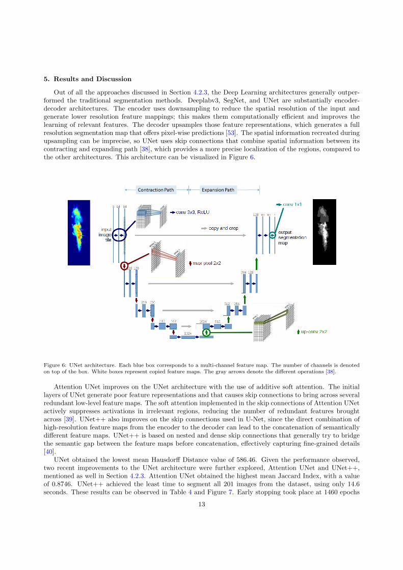
Out of all the approaches discussed in Section 4.2.3, the Deep Learning architectures generally outper-formed the traditional segmentation methods. Deeplabv3, SegNet, and UNet are substantially encoder-decoder architectures. The encoder uses downsampling to reduce the spatial resolution of the input andgenerate lower resolution feature mappings; this makes them computationally efficient and improves thelearning of relevant features. The decoder upsamples those feature representations, which generates a fullresolution segmentation map that offers pixel-wise predictions [53]. The spatial information recreated duringupsampling can be imprecise, so UNet uses skip connections that combine spatial information between itscontracting and expanding path [38], which provides a more precise localization of the regions, compared tothe other architectures. This architecture can be visualized in Figure 6.

Figure 6: UNet architecture. Each blue box corresponds to a multi-channel feature map. The number of channels is denotedon top of the box. White boxes represent copied feature maps. The gray arrows denote the different operations [38].

Attention UNet improves on the UNet architecture with the use of additive soft attention. The initiallayers of UNet generate poor feature representations and that causes skip connections to bring across severalredundant low-level feature maps. The soft attention implemented in the skip connections of Attention UNetactively suppresses activations in irrelevant regions, reducing the number of redundant features broughtacross [39]. UNet++ also improves on the skip connections used in U-Net, since the direct combination ofhigh-resolution feature maps from the encoder to the decoder can lead to the concatenation of semanticallydifferent feature maps. UNet++ is based on nested and dense skip connections that generally try to bridgethe semantic gap between the feature maps before concatenation, effectively capturing fine-grained details[40].

UNet obtained the lowest mean Hausdorff Distance value of 586.46. Given the performance observed,two recent improvements to the UNet architecture were further explored, Attention UNet and UNet++,mentioned as well in Section 4.2.3. Attention UNet obtained the highest mean Jaccard Index, with a valueof 0.8746. UNet++ achieved the least time to segment all 201 images from the dataset, using only 14.6seconds. These results can be observed in Table 4 and Figure 7. Early stopping took place at 1460 epochs

13

for UNet, at 1560 epochs for Attention UNet, and at 1055 for UNet++. The loss function values of thesemodels can be observed in Figure 8. The difference in segmentation between all the models is illustrated asan example in Figure 9.

Table 4: The mean Hausdorff Distance and Jaccard Index for all the methods mentioned in Section 4.2.3 across the testingset of 20 images. The time it took for each method to segment all 201 images from the whole data set is included in the Timecolumn, it is expressed in seconds. The best results obtained are in bold.

Method Hausdorff Distance Jaccard Index Time (s)GMM 1288.10 0.5460 2723.8

K-means 1000.63 0.5876 3035.1Thresholding 1029.08 0.6092 30.7

Chan-Vese 1031.90 0.5906 18177.5Deeplabv3 784.86 0.8502 17.1

Segnet 692.73 0.8405 16.4UNet 586.46 0.8681 15.7

Attention UNet 601.05 0.8746 17.7UNet++ 615.63 0.8722 14.6

(a) (b)

Figure 7: Box and whisker plots for the metrics of each segmentation. The values are from the result of the models mentionedin Section 4.2.3. Figure (a) shows the Hausdorff Distance results. Figure (b) shows the Jaccard Index results.

Based on these results, 300 infrared images of vertical propane jet fires were segmented by using theUNet, Attention UNet, and UNet++ models. From that segmentation, the jet flame height, L, the flamearea, A, and the lift-toff distance, S, have been obtained as shown in the Figure 4 of Section 4.1.

5.1. Flame height

The jet flame height, L, was measured from the base of the flame to the tip of the flame. In Figure 10,the flame height was plotted against the mass flow rate for all the present subsonic and sonic data, verticallyreleased into still air from four circular nozzles (i.e. 0.01275, 0.015, 0.02, and 0.03 m).

From Figure 10 it can be observed that the experimental vertical jet flames go up to 7.7 m in height, andshow a good agreement with the obtained predictions. In general, the flame height tends to increase withthe mass flow rate; however, there is some variance that reflects the turbulence of propane flames. There

14

(a) (b) (c)

Figure 8: Loss Function values of UNet, Attention UNet, and UNet++ models. Training loss is presented as a thin orangecurve, and validation loss is presented as a thick blue curve. The moment early stopping takes place is denoted as a dashedvertical red line. Figure (a) illustrates the UNet loss function values. Early stopping took place at 1460 epochs. Figure(b) illustrates the Attention UNet loss function values. Early stopping took place at 1560 epochs. Figure (c) illustrates theUNet++ loss function values. Early stopping took place at 1055 epochs.

are fewer errors visible as the diameter of the nozzle gets larger. Table 5 shows the errors of the presentexperimental jet flame heights, obtained from the segmentation of the UNet, Attention UNet, and UNet++models. The error is presented for each analyzed experiment and identified by the pipe outlet diameter. Thepresented errors are the Mean Absolute Percentage Error (MAPE) and the Root Mean Square PercentageError (RMSPE).

Table 5: The error of the flame height obtained from different segmentation models and for each experiment analysed.

HeightPipe outletdiameter (m)

0.01275 0.015 0.02 0.03

UNetMAPE 6.8% 4.5% 2.9% 2.5%RMSPE 8.7% 5.8% 3.7% 3.1%

Attention UNetMAPE 5.5% 11.1% 2.9% 2.3%RMSPE 6.7% 16.7% 3.4% 2.7%

UNet++MAPE 5.6% 11.4% 2.9% 3.3%RMSPE 7.0% 16.7% 3.6% 4.9%

For the 0.01275 m experiments, Attention UNet achieved the lowest errors and error variations, with aMAPE of 5.5% and RMSPE of 6.7%. UNet++ had a similar MAPE, but showed a higher RMSPE, denotinga higher variance in the errors.

For the 0.015 m experiments, UNet achieved the lowest errors and error variations with a MAPE of 4.5%and RMSPE of 5.8%. Attention UNet and UNet++ obtained larger errors in comparison, which mostlyhappened with the lowest and highest mass flow rates.

For the 0.02 m experiments, Attention UNet achieved the lowest errors and error variations with a MAPEof 2.9% and RMSPE of 3.4%. UNet and UNet++ obtained the same MAPE, but their RMSPE was higherin comparison, which means that the variation of the errors obtained from those models is higher.

For the 0.03 m experiments, Attention UNet achieved the lowest errors and error variations with a MAPEof 2.3% and RMSPE of 2.7%. UNet obtained a similar MAPE but higher RMSPE, and UNet++ obtainedhigher overall errors.

Attention UNet obtained the lowest MAPE and RMSPE for almost all pipe outlet diameter experiments,the only exception was the 0.015 m case. For that experiment, UNet was the best model by a high margin.This large difference mostly happens during the lowest and highest mass flow rates, where the jet fires show

15

(a) (b)

(c) (d)

(e) (f)

(g) (h)

(i) (j)

Figure 9: Sample segmentation masks. The segmentation results are obtained from the different models described in Section4.2.3. Figure (a) is the Ground Truth segmentation. Figure (b) is the Global Thresholding segmentation. Figure (c) is theK-means segmentation. Figure (d) is the Chan-Vese segmentation. Figure (e) is the Gaussian Mixture Model segmentation.Figure (f) is the DeepLabv3 segmentation. Figure (g) is the SegNet segmentation. Figure (h) is the UNet segmentation. Figure(i) is the Attention UNet segmentation. Figure (j) is the UNet++ segmentation. Slight differences can be observed along thecentral and middle zones, especially at the top and bottom parts of the flame.

16

(a) (b)

(c) (d)

Figure 10: Detected flame height for all the experiments analysed. The error bars in blue correspond to the results fromUNet, the ones in red are from Attention UNet, and the ones in green are from UNet++. Figure (a) shows the results for theexperiment with pipe outlet diameter of 0.01275 m. Figure (b) shows the results for the experiment with pipe outlet diameterof 0.015 m. Figure (c) shows the results for the experiment with pipe outlet diameter of 0.02 m. Figure (d) shows the resultsfor the experiment with pipe outlet diameter of 0.03 m.

17

sections that are detached from the main flame and add uncertainty to its limits. Attention UNet andUNet++ over-segment these parts and lead to such high errors. An example of this can be observed in Fig.11.

(a) (b)

(c) (d)

Figure 11: Example segmentation of a jet flame with outlet pipe diameter of 0.015 m and mass flow rate of 0.143 kg/s. Theextracted geometric characteristics of flame area (A), flame height (L), and lift-off distance (S) are included. Figure (a) showsthe original infrared image. Figure (b) shows the UNet segmentation results. Figure (c) shows the Attention UNet segmentationresults. Figure (d) shows the UNet++ segmentation results.

5.2. Flame area

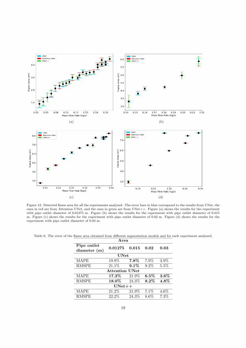
To calculate the radiation from a jet fire on a certain target, the flame area and size are required. Figure12 shows the jet flame area, A, plotted against the mass flow rate for all the present experimental data,involving the four circular nozzles of 0.01275 m, 0.015 m, 0.02 m, and 0.03 m.

From Figure 12 it can be observed that the experimental vertical jet flames reach an area of up to 8.3 m2,which is also approximated with decent accuracy by the obtained predictions. The most prominent errorsare observed in the 0.01275 m experiment; however, they seem to be consistent, which could mean that thereis a common problem that affects the general accuracy. This behavior could be explained by the turbulentnature of the flame at such a small outlet diameter. Table 6 shows the errors of the present experimental jetflame areas, obtained from the segmentation of the UNet, Attention UNet, and UNet++ models. The erroris presented for each analyzed experiment and identified by the pipe outlet diameter. The presented errorsare the Mean Absolute Percentage Error (MAPE) and the Root Mean Square Percentage Error (RMSPE).

For the 0.01275 m experiments, Attention UNet achieved the lowest errors and error variations, with aMAPE of 17.3% and RMSPE of 18.0%. As mentioned before, these are the largest errors obtained overall;

18

(a) (b)

(c) (d)

Figure 12: Detected flame area for all the experiments analysed. The error bars in blue correspond to the results from UNet, theones in red are from Attention UNet, and the ones in green are from UNet++. Figure (a) shows the results for the experimentwith pipe outlet diameter of 0.01275 m. Figure (b) shows the results for the experiment with pipe outlet diameter of 0.015m. Figure (c) shows the results for the experiment with pipe outlet diameter of 0.02 m. Figure (d) shows the results for theexperiment with pipe outlet diameter of 0.03 m.

Table 6: The error of the flame area obtained from different segmentation models and for each experiment analysed.

AreaPipe outletdiameter (m)

0.01275 0.015 0.02 0.03

UNetMAPE 19.9% 7.8% 7.9% 3.9%RMSPE 21.1% 9.1% 9.2% 5.5%

Attention UNetMAPE 17.3% 21.9% 6.5% 3.6%RMSPE 18.0% 24.3% 8.2% 4.8%

UNet++MAPE 21.2% 21.9% 7.1% 4.6%RMSPE 22.2% 24.3% 8.6% 7.3%

19

however, the small difference between the MAPE and RMSPE, shows that there is not a high variancebetween errors, alluding to a consistent problem derived from the flames in this specific case.

For the 0.015 m experiments, UNet achieved the lowest errors and error variations with a MAPE of 7.8%and RMSPE of 9.1%. Similar to what happened with the predicted height, Attention UNet and UNet++obtained larger errors in comparison, which mostly happened with the lowest mass flow rate and the twohighest mass flow rates.

For the 0.02 m experiments, Attention UNet achieved the lowest errors with a MAPE of 6.5% andRMSPE of 8.2%. UNet obtained the highest MAPE, but the lowest difference between MAPE and RMSPE,which means that it has smaller error variations.

For the 0.03 m experiments, Attention UNet achieved the lowest errors and error variations with a MAPEof 3.6% and RMSPE of 4.8%. UNet obtained a similar MAPE but higher RMSPE, and UNet++ obtainedhigher overall errors.

In a similar way to the flame height results, Attention UNet obtained the lowest MAPE and RMSPE forthe area predictions of almost all pipe outlet diameter experiments, the only exception was the 0.015 m case.For that experiment, UNet was the best model by a high margin. The area was the geometric characteristicthat obtained the highest errors for the experiments presented in this paper; however, this can be explainedby how the experimental area is usually obtained from a minimum bounding box. By segmenting the flame,the areas without flame that may have been included in the minimum bounding box are excluded from theprediction. Even so, the highest error still allows for an approximate representation of the experimentalarea.

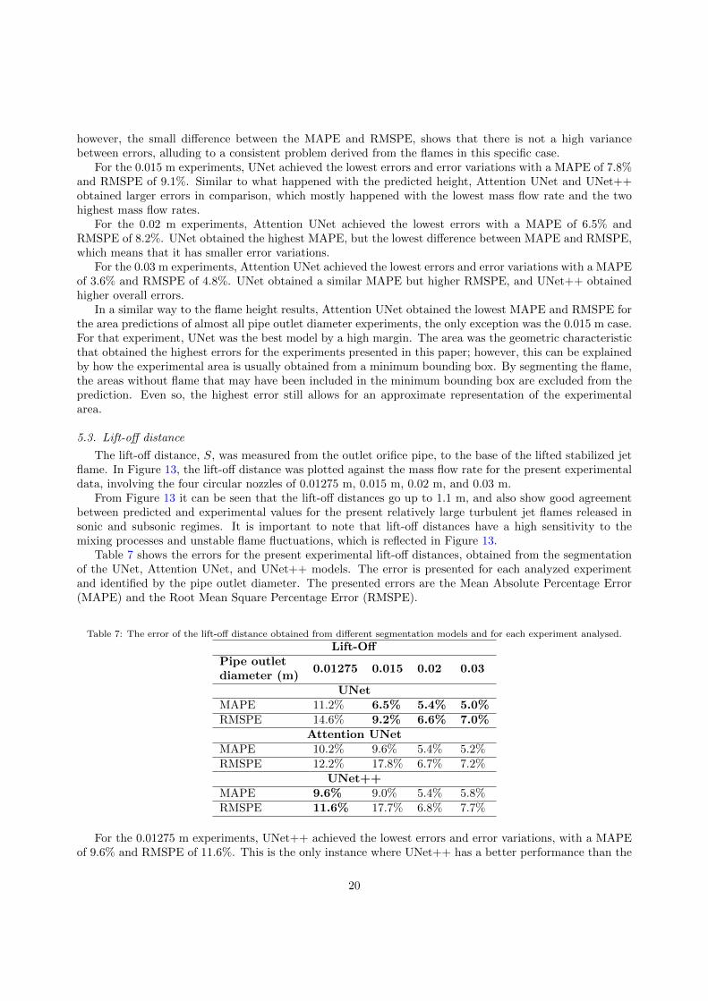
5.3. Lift-off distance

The lift-off distance, S, was measured from the outlet orifice pipe, to the base of the lifted stabilized jetflame. In Figure 13, the lift-off distance was plotted against the mass flow rate for the present experimentaldata, involving the four circular nozzles of 0.01275 m, 0.015 m, 0.02 m, and 0.03 m.

From Figure 13 it can be seen that the lift-off distances go up to 1.1 m, and also show good agreementbetween predicted and experimental values for the present relatively large turbulent jet flames released insonic and subsonic regimes. It is important to note that lift-off distances have a high sensitivity to themixing processes and unstable flame fluctuations, which is reflected in Figure 13.

Table 7 shows the errors for the present experimental lift-off distances, obtained from the segmentationof the UNet, Attention UNet, and UNet++ models. The error is presented for each analyzed experimentand identified by the pipe outlet diameter. The presented errors are the Mean Absolute Percentage Error(MAPE) and the Root Mean Square Percentage Error (RMSPE).

Table 7: The error of the lift-off distance obtained from different segmentation models and for each experiment analysed.

Lift-OffPipe outletdiameter (m)

0.01275 0.015 0.02 0.03

UNetMAPE 11.2% 6.5% 5.4% 5.0%RMSPE 14.6% 9.2% 6.6% 7.0%

Attention UNetMAPE 10.2% 9.6% 5.4% 5.2%RMSPE 12.2% 17.8% 6.7% 7.2%

UNet++MAPE 9.6% 9.0% 5.4% 5.8%RMSPE 11.6% 17.7% 6.8% 7.7%

For the 0.01275 m experiments, UNet++ achieved the lowest errors and error variations, with a MAPEof 9.6% and RMSPE of 11.6%. This is the only instance where UNet++ has a better performance than the

20

(a) (b)

(c) (d)

Figure 13: Detected lift-off distance for all the experiments analysed. The error bars in blue correspond to the results fromUNet, the ones in red are from Attention UNet, and the ones in green are from UNet++. Figure (a) shows the results for theexperiment with pipe outlet diameter of 0.01275 m. Figure (b) shows the results for the experiment with pipe outlet diameterof 0.015 m. Figure (c) shows the results for the experiment with pipe outlet diameter of 0.02 m. Figure (d) shows the resultsfor the experiment with pipe outlet diameter of 0.03 m.

21

other two models. Attention UNet has a slightly higher MAPE, but it obtains the same difference betweenMAPE and RMSPE as the UNet++ results, which means that they have similar error variations.

For the 0.015 m experiments, UNet achieved the lowest errors and error variations with a MAPE of 6.5%and RMSPE of 9.2%. Similar to what happened with the predicted height and area, Attention UNet andUNet++ obtained larger errors in comparison, which mostly happened with the lowest mass flow rate.

For the 0.02 m experiments, UNet achieved the lowest errors with a MAPE of 5.4% and RMSPE of6.6%. Attention UNet and UNet++ obtained the same MAPE, but slightly higher RMSPE, which meansthat they present a higher error variation.

For the 0.03 m experiments, UNet achieved the lowest errors and error variations with a MAPE of5.0% and RMSPE of 7.0%. Attention UNet and UNet++ obtained slightly higher MAPE but relativelyhomogeneous differences between MAPE and RMSPE, which means that they all presented similar errorvariances.

The lift-off distance presented a large variance between errors, which can be explained by the turbulenceof these open field flames. Contrary to the flame height and area results, UNet obtained the lowest MAPEand RMSPE for the lift-off distance predictions of almost all pipe outlet diameter experiments, the onlyexception was the 0.01275 m case; for that experiment, UNet++ was the best model.

5.4. Statistical test

It can be visualized from Fig. 14 that all three models show some deviation from normality, especially atthe start and end of the data. This means that our initial assumptions were correct, thus the application ofa non-parametric paired statistical test is the best approach. The resulting p-values of the Wilcoxon signedrank test can be summarized in Table 8.

(a) (b) (c)

Figure 14: UNet, Attention UNet, and UNet++ Q-Q plots. The plots illustrate the deviations of the errors from a normaldistribution. Figure (a) is the UNet Q-Q plot. Figure (b) is the Attention UNet Q-Q plot. Figure (c) is the UNet++ Q-Q plot.

Table 8: Resulting p-value from the Wilcoxon signed rank tests between models.

Comparison p-valueUNet and Attention UNet 0.8753UNet and UNet++ 0.2094Attention UNet and UNet++ 0.0844

The highest p-value is obtained when comparing the MAPE of UNet and Attention UNet, which meansthat there is not enough data to reject the null hypothesis; and therefore, show a statistically significantdifference to suggest one model over the other. This result matches the observed behavior where UNetwould surpass Attention UNet by a high margin only on specific cases, mostly while extracting the flameheight and flame area from experiments with a pipe outlet diameter of 0.015 m, during low and high massflow rates.

The second highest p-value was obtained when comparing the MAPE of UNet and UNet++. Even ifthe p-value is notably lower, it remains over the established significance level, so there is not enough data

22

to show a statistically significant difference between the models. This result goes along with the perceivederrors of the specific case where UNet++ would only surpass UNet while extracting the lift-off distance fromexperiments with a pipe outlet diameter of 0.01275 m.

Finally, the lowest p-value is observed in the comparison between the MAPE of Attention UNet andUNet++, which is also lower than the established significance level of 0.1. This means that there is astatistically significant difference between these two models. In this case, it is recommended Attention UNetover UNet++, since the only instances where UNet++ surpassed Attention UNet happened while extractingthe lift-off distance from experiments with a pipe outlet diameter of 0.01275 and 0.015 m. However, evenin those cases, the difference between the errors is minimal. In the experiments with a pipe outlet diameterof 0.01275 m, the difference between errors is only 0.6 for both MAPE and RMSPE. In the experimentswith a pipe outlet diameter of 0.015 m, the difference between MAPE is also 0.6, but the difference betweenRMSPE is only 0.1.

6. Conclusions

This research work explores the application of deep learning models in an alternative approach that usesthe semantic segmentation of jet fires flames to extract the flame’s main geometrical attributes, relevant forfire risk analyses. To the best of our knowledge, this is the first work to present a comparative study forthis approach, between traditional computer vision algorithms and certain deep learning algorithms fromthe state-of-the-art. The major findings of this study can be summarized as follows:

1. Between the analyzed traditional image processing methods and the state-of-the-art deep learningmodels, the best results for the segmentation of jet fires were given by the deep learning architectureUNet, along with two recent improvements on it, namely Attention UNet and UNet++. UNet obtainedthe best Hausdorff Distance, Attention UNet achieved the best Jaccard Index, and UNet++ took theleast time to segment all 201 images from the dataset.

2. Compared to other traditional algorithms, Deep Learning models automatically detect the most de-scriptive and salient features for the problem. In contrast to the other Deep Learning architecturesexplored, UNet offers precise localization of the regions and a good definition of their borders. This ispossible because of the skip connections that combine spatial information between its contracting andexpanding path. This architecture, however, takes a significant amount of time to train and can leavehigh GPU memory footprints when dealing with larger images.

3. Both Attention UNet and UNet++ improve on the UNet architecture. Attention UNet reduces thenumber of redundant feature maps brought across by skip connections, and UNet++ bridges thesemantic gap between feature maps before their concatenation. These improvements, however, increasethe number of parameters, which also significantly increment the training time of the models.

4. The height of the flames is approximated from the segmentation performed by the UNet, AttentionUNet, and UNet++ models. For the experiments with a pipe outlet diameter of 0.01275 m, 0.02 m,and 0.3 m, Attention UNet obtained the best results, with a maximum MAPE of 5.5%, and a minimumof 2.3%. For the experiment with a pipe outlet diameter of 0.015 m, UNet obtained the best result,with a MAPE of 4.5%.

5. The area of the flames is approximated from the segmentation performed by the UNet, AttentionUNet, and UNet++ models. For the experiments with a pipe outlet diameter of 0.01275 m, 0.02m, and 0.3 m, Attention UNet obtained the best results, with a maximum MAPE of 17.3%, and aminimum of 3.6%. For the experiment with a pipe outlet diameter of 0.015 m, UNet obtained the bestresult, with a MAPE of 7.8%.

6. The lift-off distances of the flames are approximated from the segmentation performed by the UNet,Attention UNet, and UNet++ models. For the experiments with a pipe outlet diameter of 0.015 m,0.02 m, and 0.3 m, UNet obtained the best results, with a maximum MAPE of 6.5%, and a minimumof 5.0%. For the experiment with a pipe outlet diameter of 0.01275 m, UNet++ obtained the bestresult, with a MAPE of 9.6%. This is the only instance where UNet++ outperforms the other models.

23

7. Among the three different geometric characteristics of jet fires analyzed in this paper, the area resultedin the highest errors from the validation experiments. This, however, can be explained by how theexperimental area is usually approximated from a minimum bounding box, which usually includesareas without flame that are excluded from the segmentation’s prediction. Even so, the highest overallMAPE of 21.9% still allows for a decent representation of the experimental area.

8. Based on the results obtained from the Wilcoxon signed rank test to compare the models’ MAPE, itcan be concluded that the Attention UNet model has a better performance than the UNet++ model;since there is a statistically significant difference between them. However, the same cannot be saidfor the UNet model, which does not show a statistically significant difference between Attention UNetand UNet++. Further experiments and data would be necessary to show this.

9. Bearing all these results in mind, the usage of Attention UNet for general characterization could berecommended; however, further testing with UNet is also recommended for the case of lift-off distances.

It is important to mention that the Deep Learning models were trained with a data set of 201 images,and using a larger data set could significantly increase the accuracy and statistically significant difference ofthe UNet, Attention UNet, and UNet++ architectures. Furthermore, it is important to highlight that thesegmentation obtained from the current models can also be used to classify different radiation zones withinthe flame with their respective temperature and geometry. The information from this characterization couldbe used along with other models, such as a Weighted Multi Point Source model or a Computational FluidDynamics model. This would allow for a more thorough risk analysis of jet fires that evaluates the likelihoodof direct flame impingement and determines the distribution and intensity of radiant heat that is emittedfrom the flame to the surrounding equipment.

As future work, other improved versions of the Deep Learning architectures could be tested and differentreal-time algorithms could be explored to further improve the efficiency and accuracy of the segmentation.Additionally, the application of edge computing, smart cameras, or 8-bit quantization, could be introducedto use fewer bits for calculation and storage, which would accelerate the processing time of these algorithms.The experiment could also be redesigned for a more controlled benchmark to compare to other algorithms inthe literature and future studies on the problem of fire segmentation. Taking all this into consideration, theresearch presented is a promising first step toward a fast and reliable risk management system for generalfire incidents.

7. Acknowledgments

This work was supported through a scholarship for Carmina Perez-Guerrero by the Mexican NationalCouncil of Science and Technology (CONACYT). This research is part of the project 7817-2019 funded bythe Jalisco State Council of Science and Technology (COECYTJAL).

References

[1] M. Gomez-Mares, L. Zarate, J. Casal, Jet fires and the domino effect, Fire Safety Journal 43 (8) (2008) 583–588. doi:

10.1016/j.firesaf.2008.01.002.[2] G. T. Kalghatgi, Lift-off heights and visible lengths of vertical turbulent jet diffusion flames in still air, Combustion Science

and Technology 41 (1-2) (1984) 17–29. doi:10.1080/00102208408923819.[3] D. Bradley, P. H. Gaskell, X. Gu, A. Palacios, Jet flame heights, lift-off distances, and mean flame surface density for

extensive ranges of fuels and flow rates, Combustion and Flame 164 (2016) 400–409. doi:10.1016/j.combustflame.2015.09.009.

[4] T. Guiberti, W. Boyette, W. Roberts, Height of turbulent non-premixed jet flames at elevated pressure, Combustion andFlame 220 (2020) 407–409. doi:10.1016/j.combustflame.2020.07.010.

[5] A. Palacios, J. Casal, Assessment of the shape of vertical jet fires, Fuel 90 (2) (2011) 824–833. doi:10.1016/j.fuel.2010.09.048.

[6] X. Zhang, L. Hu, Q. Wang, X. Zhang, P. Gao, A mathematical model for flame volume estimation based on flame heightof turbulent gaseous fuel jet, Energy Conversion and Management 103 (2015) 276–283. doi:10.1016/j.enconman.2015.

06.061.[7] Z. Wang, K. Zhou, L. Zhang, X. Nie, Y. Wu, J. Jiang, A. S. Dederichs, L. He, Flame extension area and temperature

profile of horizontal jet fire impinging on a vertical plate, Process Safety and Environmental Protection 147 (2021) 547–558.doi:10.1016/j.psep.2020.11.028.

24

[8] Z. Wang, K. Zhou, M. Liu, Y. Wang, X. Qin, J. Jiang, Lift-off behavior of horizontal subsonic jet flames impinging ona cylindrical surface, Proceedings of the Ninth International Seminar on Fire and Explosion Hazards 2 (2019) 21–26.doi:10.18720/SPBPU/2/k19-79.

[9] F. Colella, A. Ibarreta, R. J. Hart, T. Morrison, H. A. Watson, M. Yen, Jet fire consequence analysis, OTC OffshoreTechnology Conference (2020). doi:10.4043/30802-MS.

[10] H. Mashhadimoslem, A. Ghaemi, A. Palacios, Analysis of deep learning neural network combined with experiments todevelop predictive models for a propane vertical jet fire, Heliyon 6 (11) (2020) e05511. doi:10.1016/j.heliyon.2020.

e05511.[11] G. Litjens, T. Kooi, B. E. Bejnordi, A. A. A. Setio, F. Ciompi, M. Ghafoorian, J. A. van der Laak, B. van Ginneken,

C. I. Sanchez, A survey on deep learning in medical image analysis, Medical Image Analysis 42 (2017) 60–88. doi:

10.1016/j.media.2017.07.005.[12] X. Chang, H. Pan, W. Sun, H. Gao, Yoltrack: Multitask learning based real-time multiobject tracking and segmentation

for autonomous vehicles, IEEE Transactions on Neural Networks and Learning Systems PP (99) (2021) 1–11. doi:

10.1109/TNNLS.2021.3056383.[13] C. Xie, Y. Xiang, A. Mousavian, D. Fox, Unseen object instance segmentation for robotic environments, IEEE Transactions

on Robotics 37 (2021) 1343–1359. doi:10.1109/TRO.2021.3060341.[14] B. Zhang, J. Zhang, A traffic surveillance system for obtaining comprehensive information of the passing vehicles based

on instance segmentation, IEEE Transactions on Intelligent Transportation Systems PP (99) (2020) 1–16. doi:10.1109/

TITS.2020.3001154.[15] S. Liu, L. Qi, H. Qin, J. Shi, J. Jia, Path aggregation network for instance segmentation, IEEE. CVF Conference on

Computer Vision and Pattern Recognition 1 (2018) 8759–8768. doi:10.1109/CVPR.2018.00913.[16] K. Khan, R. U. Khan, K. Ahmad, F. Ali, K.-S. Kwak, Face segmentation: A journey from classical to deep learning

paradigm, approaches, trends, and directions, IEEE Access 8 (2020) 58683–58699. doi:10.1109/ACCESS.2020.2982970.[17] S. A. Taghanaki, K. Abhishek, J. P. Cohen, J. Cohen-Adad, G. Hamarneh, Deep semantic segmentation of natural and

medical images: a review, Artificial Intelligence Review 54 (1) (2020) 137–78. doi:10.1007/s10462-020-09854-1.[18] L. Chan, M. S. Hosseini, K. N. Plataniotis, A comprehensive analysis of weakly-supervised semantic segmentation in differ-

ent image domains, International Journal of Computer Vision 129 (2) (2020) 361–84. doi:10.1007/s11263-020-01373-4.

[19] A. Troya-Galvis, P. Gancarski, L. Berti-Equille, Collaborative segmentation and classification for remote sensing imageanalysis, in: International Conference on Pattern Recognition, Vol. 23, 2016, pp. 829–834. doi:10.1109/ICPR.2016.

7899738.[20] P. A. Croce, K. S. Mudan, Calculating impacts for large open hydrocarbon fires, Fire Safety Journal 11 (1) (1986) 99–112.

doi:https://doi.org/10.1016/0379-7112(86)90055-X.[21] G. A. Chamberlain, Developments in design methods for predicting thermal radiation from flares, Chemical Engineering

Research and Design 65 (4) (1987).[22] K. Zhou, J. Jiang, Thermal radiation from vertical turbulent jet flame: Line source model, Journal of Heat Transfer

138 (4) (2015). doi:10.1115/1.4032151.[23] L. Quezada, P. Pagot, F. Franca, F. Pereira, Experimental study of jet fire radiation and a new approach for optimizing

the weighted multi-point source model by inverse methods, Fire Safety Journal 113 (2020) 102972. doi:https://doi.org/10.1016/j.firesaf.2020.102972.

[24] E. Kashi, M. Bahoosh, Jet fire assessment in complex environments using computational fluid dynamics, Brazilian Journalof Chemical Engineering 37 (2020) 203 – 212. doi:10.1007/s43153-019-00003-y.

[25] R. Janssen, N. Sepasian, Automatic flare-stack monitoring, SPE Production & Operations 34 (01) (2018) 18–23. doi:

10.2118/187257-PA.[26] J. Zhu, W. Li, D. Lin, H. Cheng, G. Zhao, Intelligent fire monitor for fire robot based on infrared image feedback control,

Fire Technology 56 (5) (2020) 2089–2109. doi:10.1007/s10694-020-00964-4.[27] S. Yuheng, Y. Hao, Image segmentation algorithms overview, CoRR 1707.02051 (2017). arXiv:1707.02051.[28] K. Gu, Y. Zhang, J. Qiao, Vision-based monitoring of flare soot, IEEE Transactions on Instrumentation and Measurement

69 (9) (2020) 7136–7145. doi:10.1109/TIM.2020.2978921.[29] S. Rudz, K. Chetehouna, A. Hafiane, H. Laurent, O. Sero-Guillaume, Investigation of a novel image segmentation method

dedicated to forest fire applications, Measurement Science and Technology 24 (7) (2013) 075403. doi:10.1088/0957-0233/24/7/075403.

[30] M. Ajith, M. Martınez-Ramon, Unsupervised segmentation of fire and smoke from infra-red videos, IEEE Access 7 (2019)182381–182394. doi:10.1109/ACCESS.2019.2960209.

[31] N. M. Zaitoun, M. J. Aqel, Survey on image segmentation techniques, Procedia Computer Science 65 (2015) 797–806.doi:10.1016/j.procs.2015.09.027.

[32] M. Roberts, J. Spencer, Chan–vese reformulation for selective image segmentation, Journal of Mathematical Imaging andVision 61 (8) (2019) 1173–1196. doi:10.1007/s10851-019-00893-0.

[33] D. Zhou, H. Zhou, Y. Shao, An improved chan–vese model by regional fitting for infrared image segmentation, InfraredPhysics & Technology 74 (2016) 81–88. doi:10.1016/j.infrared.2015.12.003.

[34] N. O. Mahony, S. Campbell, A. Carvalho, S. Harapanahalli, G. A. Velasco-Hernandez, L. Krpalkova, D. Riordan, J. Walsh,Deep learning vs. traditional computer vision, Advances in Intelligent Systems and Computing 943 (2019) 128–144.doi:10.1007/978-3-030-17795-9_10.

[35] Z. Mingwei, W. Jing, J. Lin, N. Fang, W. Wei, M. Wozniak, R. Damasevicius, Nas-hris: Automatic design and architecturesearch of neural network for semantic segmentation in remote sensing images, Sensors 20 (2020) 5292. doi:10.3390/

s20185292.

25

[36] L. Chen, G. Papandreou, I. Kokkinos, K. Murphy, A. L. Yuille, Deeplab: Semantic image segmentation with deepconvolutional nets, atrous convolution, and fully connected crfs, IEEE Transactions on Pattern Analysis and MachineIntelligence 40 (4) (2018) 834–848. doi:10.1109/TPAMI.2017.2699184.

[37] V. Badrinarayanan, A. Kendall, R. Cipolla, Segnet: A deep convolutional encoder-decoder architecture for imagesegmentation, IEEE Transactions on Pattern Analysis and Machine Intelligence 39 (12) (2017) 2481–2495. doi:

10.1109/TPAMI.2016.2644615.[38] O. Ronneberger, P. Fischer, T. Brox, U-net: Convolutional networks for biomedical image segmentation, Medical Image

Computing and Computer-Assisted Intervention 9351 (2015) 234–241. doi:10.1007/978-3-319-24574-4_28.[39] O. Oktay, J. Schlemper, L. L. Folgoc, M. Lee, M. Heinrich, K. Misawa, K. Mori, S. McDonagh, N. Y. Hammerla, B. Kainz,

B. Glocker, D. Rueckert, Attention u-net: Learning where to look for the pancreas (2018). arXiv:1804.03999.[40] Z. Zhou, M. M. R. Siddiquee, N. Tajbakhsh, J. Liang, Unet++: Redesigning skip connections to exploit multiscale features

in image segmentation, IEEE Transactions on Medical Imaging (2019). doi:10.1109/TMI.2019.2959609.[41] A. Palacios, Study of jet fires geometry and radiative features, Ph.D. thesis, Universitat Politecnica de Catalunya (2011).

[42] V. Foroughi, A. Palacios, C. Barraza, A. Agueda, C. Mata, E. Pastor, J. Casal, Thermal effects of a sonic jet fireimpingement on a pipe, Journal of Loss Prevention in the Process Industries 71 (2021) 104449. doi:10.1016/j.jlp.2021.104449.

[43] M. Gomez-Mares, M. Munoz, J. Casal, Axial temperature distribution in vertical jet fires, Journal of Hazardous Materials172 (1) (2009) 54–60. doi:10.1016/j.jhazmat.2009.06.136.

[44] A. A. Taha, A. Hanbury, Metrics for evaluating 3d medical image segmentation: Analysis, selection, and tool, BMCMedical Imaging 15 (29) (2015) 15–29. doi:10.1186/s12880-015-0068-x.

[45] C. Perez-Guerrero, A. Palacios, G. Ochoa-Ruiz, C. Mata, M. Gonzalez-Mendoza, L. E. Falcon-Morales, Comparing machinelearning based segmentation models on jet fire radiation zones, in: Advances in Computational Intelligence. MICAI 2021.Lecture Notes in Computer Science, Vol. 13067, Springer International Publishing, 2021, pp. 161–172. doi:10.3390/

s16101756.[46] G. Klanderman, W. Rucklidge, D. Huttenlocher, Comparing images using the hausdorff distance, IEEE Transactions on

Pattern Analysis & Machine Intelligence 15 (09) (1993) 850–863. doi:10.1109/34.232073.[47] M. Rahman, Y. Wang, Optimizing intersection-over-union in deep neural networks for image segmentation, in: 12th

International Symposium on Visual Computing, Vol. 10072, 2016, pp. 234–244. doi:10.1007/978-3-319-50835-1_22.[48] M. Shcherbakov, A. Brebels, N. Shcherbakova, A. Tyukov, T. Janovsky, V. Kamaev, A survey of forecast error measures,

World Applied Sciences Journal 24 (2013) 171–176. doi:10.5829/idosi.wasj.2013.24.itmies.80032.[49] M. G. Ben, V. J. Yohai, Quantile–quantile plot for deviance residuals in the generalized linear model, Journal of Compu-

tational and Graphical Statistics 13 (1) (2004) 36–47. doi:10.1198/1061860042949_a.[50] I. C. A. Oyeka, G. U. Ebuh, Modified wilcoxon signed-rank test, Open Journal of Statistics 02 (2) (2012) 172–176.

doi:10.4236/ojs.2012.22019.[51] P. Getreuer, Chan-vese segmentation, Image Processing On Line 2 (2012) 214–224. doi:10.5201/ipol.2012.g-cv.[52] A. Paszke, A. Chaurasia, S. Kim, E. Culurciello, Enet: A deep neural network architecture for real-time semantic segmen-

tation, arXiv (2016). arXiv:1606.02147.[53] Y. Xing, L. Zhong, X. Zhong, An encoder-decoder network based fcn architecture for semantic segmentation, Wireless

Communications and Mobile Computing (2020) 1–9doi:10.1155/2020/8861886.

26