Embed Size (px)
Citation preview

BIROn - Birkbeck Institutional Research Online
Enabling Open Access to Birkbeck’s Research Degree output
Explainable credit scoring through generative adver-sarial networks
https://eprints.bbk.ac.uk/id/eprint/47370/
Version: Full Version
Citation: Han, Seongil (2021) Explainable credit scoring through gener-ative adversarial networks. [Thesis] (Unpublished)
c© 2020 The Author(s)
All material available through BIROn is protected by intellectual property law, including copy-right law.Any use made of the contents should comply with the relevant law.
Deposit GuideContact: email

Explainable Credit Scoring
through
Generative Adversarial Networks
by
Seongil Han
Department of Computer Science and Information Systems
Birkbeck College, University of London
Malet Street, London, WC1E 7HX
United Kingdom
Email: [email protected]
29 September 2021
Thesis submitted in the fulfillment of the
requirements for the degree of Doctor of
Philosophy (PhD) in Computer Science and
Information Systems in University of London

Abstract
Credit scoring has been playing a vital role in mitigating financial risk that
could affect the sustainability of financial institutions. An accurate and au-
tomated credit scoring allows to control the financial risk by using the state-
of-the-art and data-driven analytics.
The primary rationale of this thesis is to understand and improve fi-
nancial credit scoring models. The key issues that occur in the process of
developing credit scoring model using the state-of-the-art machine learning
(ML) techniques, are identified and investigated. Through the proposed mod-
els using ML approaches in this thesis, the challenges in credit scoring can be
resolved. Therefore, the existing credit scoring models can be improved by
novel computer science techniques in realistic problem of the areas as follows.
First, an interpretability aspect of credit scoring as eXplainable Artifi-
cial Intelligence (XAI) is examined by non-parametric tree-based ML models
combining with SHapley Additive exPlanations (SHAP). In this experiment,
the suitability of tree-based ensemble models is also assessed in imbalanced
credit scoring dataset, comparing the performance of different class imbal-
ance. In order to achieve explainability as well as high predictive perfor-
mance in credit scoring, we propose a model named as NATE which is Non-
pArameTric approach for Explainable credit scoring. This explainable and
comprehensible NATE allows us to analyse the key factors of credit scoring
by SHAP values both locally and globally in addition to robust predictive
power for creditworthiness.
1

Second, the issue of class imbalance is investigated. Class imbalance in
datasets occurs when there are a huge number of differences of observations
between the classes in the dataset. The imbalanced class in real-world credit
scoring datasets results in the biased classification performance for creditwor-
thiness. As an approach to overcome the limitation of traditional resampling
methods for class imbalance, we propose a model named as NOTE which is
Non-parametric Oversampling Techniques for Explainable credit scoring. By
using conditional Wasserstein Generative Adversarial Networks (cWGAN)-
based oversampling technique paired with Non-parametric Stacked Autoen-
coder (NSA), NOTE as a generative model allows to oversample minority
class with reflecting the complex and non-linear patterns in the dataset.
Therefore, NOTE predicts the classification and explains the credit scoring
model with unbiased performance on a balanced credit scoring dataset.
Third, incomplete data is also a common issue in credit scoring datasets.
This missingness normally distorts the analysis and prediction for credit scor-
ing, and results in the misclassification for creditworthiness. To address the
issue of missing values in the dataset and overcome the limitation of con-
ventional imputation methods, we propose a model named as DITE which is
Denoising Imputation TEchniques for missingness in credit scoring. By using
the extended Generative Adversarial Imputation Networks (GAIN) paired
with randomised Singular Value Decomposition (rSVD), DITE is capable of
replacing missing values with plausible estimation through reducing the noise
and capturing complex missing patterns in dataset.
To evaluate the robustness and effectiveness of the proposed models
for key issues, namely, model explainability, class imbalance, and missing-
ness in the dataset, the performances of models using ML are compared
against the benchmarks of literature on publicly available real-world finan-
cial credit scoring datasets, respectively. Our experimental results success-
fully demonstrated the robustness and effectiveness of the novel concepts
used in the models by outperforming the benchmarks. Furthermore, the pro-
posed NATE, NOTE and DITE also lead to a better model explainability,
suitability, stability, and superiority on complex and non-linear credit scoring
2

datasets. Finally, this thesis demonstrated that the existing credit scoring
models can be improved by novel computer science techniques in real-world
problem of credit scoring domain.
This research has been supervised by Dr Andrea Calı and Dr Alessandro
Provetti.
3

Declaration
I, Seongil Han, confirm that this thesis and the work presented in it are my
own. I also confirm that all the information derived from other sources has
been cited and acknowledged within the thesis.
Signature:
Date:
4

Acknowledgements
I would like to express my deepest gratitude to following people who have
supported my PhD journey.
First, I would like to thank my principal supervisors, Dr. Andrea Calı
and Dr. Alessandro Provetti, for their wonderful guidance, support, trust
and expertise. Andrea Cali and Alessandro Provetti were excellent mentors.
Second, I would like to thank my advisory supervisor, Dr. Paul D. Yoo, for
his invaluable feedback, advice, encouragement and support throughout the
projects. Paul D. Yoo was a superb motivator. Third, I would like to thank
colleagues at Birkbeck Institute for Data Analytics and Birkbeck Knowledge
Lab in MAL159 for your friendship.
Finally, I record my special thanks to my wife Suhlim for her love. I
could not have done this journey without her support.
5

Contents
1 Introduction 16
1.1 Background . . . . . . . . . . . . . . . . . . . . . . . . . . . . 16
1.2 Motivation . . . . . . . . . . . . . . . . . . . . . . . . . . . . . 19
1.3 Contributions . . . . . . . . . . . . . . . . . . . . . . . . . . . 24
1.4 Outline . . . . . . . . . . . . . . . . . . . . . . . . . . . . . . . 27
1.5 Publications . . . . . . . . . . . . . . . . . . . . . . . . . . . . 28
2 Machine Learning 30
2.1 Concepts . . . . . . . . . . . . . . . . . . . . . . . . . . . . . . 30
2.1.1 The Learning Process . . . . . . . . . . . . . . . . . . . 31
2.1.2 The Hypothesis Space . . . . . . . . . . . . . . . . . . 32
2.2 Evaluation and Selection for Models . . . . . . . . . . . . . . . 33
2.2.1 Error and Overfitting . . . . . . . . . . . . . . . . . . . 33
2.2.2 Performance Measures . . . . . . . . . . . . . . . . . . 36
2.3 Classification Algorithms . . . . . . . . . . . . . . . . . . . . . 42
2.3.1 Basic Form of Linear Models . . . . . . . . . . . . . . . 42
2.3.2 Logistic Regression . . . . . . . . . . . . . . . . . . . . 43
6

2.3.3 Decision Tree . . . . . . . . . . . . . . . . . . . . . . . 46
2.3.4 Ensemble Models . . . . . . . . . . . . . . . . . . . . . 48
2.3.5 Neural Network . . . . . . . . . . . . . . . . . . . . . . 54
3 Credit Scoring 58
3.1 Concepts . . . . . . . . . . . . . . . . . . . . . . . . . . . . . . 58
3.2 Modelling . . . . . . . . . . . . . . . . . . . . . . . . . . . . . 61
3.3 Credit Scoring Datasets . . . . . . . . . . . . . . . . . . . . . 64
3.3.1 Preconditions of Datasets . . . . . . . . . . . . . . . . 64
3.3.2 Collection of Datasets . . . . . . . . . . . . . . . . . . 64
3.3.3 Preprocessing of Datasets . . . . . . . . . . . . . . . . 67
3.4 Summary for Designing Proposed Credit Scoring Model . . . . 73
3.5 Explainable Models: Parametric vs Non-parametric . . . . . . 73
3.6 Class Imbalance . . . . . . . . . . . . . . . . . . . . . . . . . . 75
3.7 Missing Values . . . . . . . . . . . . . . . . . . . . . . . . . . 78
4 Non-parametric Approach for Explainable Credit Scoring on
Imbalanced Class 80
4.1 Introduction . . . . . . . . . . . . . . . . . . . . . . . . . . . . 80
4.2 Related Work . . . . . . . . . . . . . . . . . . . . . . . . . . . 83
4.2.1 Explainability as XAI in Credit Scoring . . . . . . . . . 83
4.2.2 Ensemble Approach with Oversampling Techniques in
Credit Scoring . . . . . . . . . . . . . . . . . . . . . . . 86
4.3 NATE: Non-pArameTric approach for Explainable credit scor-
ing on imbalanced class . . . . . . . . . . . . . . . . . . . . . . 88
7

4.4 Results . . . . . . . . . . . . . . . . . . . . . . . . . . . . . . . 99
4.4.1 Benchmarks on the Original Dataset . . . . . . . . . . 99
4.4.2 Performance Comparison on Resampled Dataset . . . . 101
4.4.3 Performance Comparison: Undersampling vs Oversam-
pling . . . . . . . . . . . . . . . . . . . . . . . . . . . . 104
4.4.4 Interpretability of Predictions . . . . . . . . . . . . . . 106
4.5 Conclusion . . . . . . . . . . . . . . . . . . . . . . . . . . . . . 109
5 GAN-based Oversampling Techniques for Imbalanced Class111
5.1 Introduction . . . . . . . . . . . . . . . . . . . . . . . . . . . . 111
5.2 Related Work . . . . . . . . . . . . . . . . . . . . . . . . . . . 114
5.2.1 GAN-based Oversampling . . . . . . . . . . . . . . . . 114
5.2.2 Generating Tabular Data by GAN . . . . . . . . . . . 116
5.3 NOTE: Non-parametric Oversampling Techniques for Explainable
credit scoring . . . . . . . . . . . . . . . . . . . . . . . . . . . 117
5.4 Results . . . . . . . . . . . . . . . . . . . . . . . . . . . . . . . 129
5.4.1 The Generative Performance . . . . . . . . . . . . . . . 129
5.4.2 The Predictive Performance . . . . . . . . . . . . . . . 132
5.5 Conclusion . . . . . . . . . . . . . . . . . . . . . . . . . . . . . 139
6 GAN-based Imputation Techniques for Missing Values 141
6.1 Introduction . . . . . . . . . . . . . . . . . . . . . . . . . . . . 141
6.2 Related Work . . . . . . . . . . . . . . . . . . . . . . . . . . . 144
6.2.1 Imputation Methods for Missing Values . . . . . . . . . 144
6.2.2 Mechanism for Missing Values . . . . . . . . . . . . . . 147
8

6.3 DITE: Denoising Imputation TEchniques for missingness in
credit scoring . . . . . . . . . . . . . . . . . . . . . . . . . . . 149
6.4 Results . . . . . . . . . . . . . . . . . . . . . . . . . . . . . . . 157
6.5 Conclusion . . . . . . . . . . . . . . . . . . . . . . . . . . . . . 161
7 Conclusions 163
7.1 Introduction . . . . . . . . . . . . . . . . . . . . . . . . . . . . 163
7.2 Summary of Contributions . . . . . . . . . . . . . . . . . . . . 164
7.3 Future Work . . . . . . . . . . . . . . . . . . . . . . . . . . . . 167
A Abbreviations 169
B Additional materials for NOTE 172
References 175
9

List of Figures
1.1 The number of studies for balancing datasets in credit scoring
models (Dastile et al., 2020) . . . . . . . . . . . . . . . . . . . 22
2.1 10-fold cross-validation . . . . . . . . . . . . . . . . . . . . . . 35
2.2 Confusion matrix for credit scoring, where good means good
credit or not defaulted, and bad means bad credit or defaulted 38
2.3 An example of ROC curve . . . . . . . . . . . . . . . . . . . . 41
2.4 The number of studies for evaluating performance in credit
scoring models (Dastile et al., 2020) . . . . . . . . . . . . . . . 42
2.5 Linear model and logistic curve . . . . . . . . . . . . . . . . . 44
2.6 A hypothetical example of DT model in credit scoring . . . . . 47
2.7 The structure of parallel and sequential ensemble . . . . . . . 49
2.8 The structure of random forest . . . . . . . . . . . . . . . . . 50
2.9 The structure of neural network with four inputs (features)
x1, x2, x3, x4, two outputs y1, y2, and n hidden layers . . . . . . 55
3.1 The process of credit scoring . . . . . . . . . . . . . . . . . . . 60
3.2 The general framework for credit scoring using ML models . . 62
3.3 Missing values in features on credit scoring datasets (GMSC,
HE, and DC in order) . . . . . . . . . . . . . . . . . . . . . . 68
10

3.4 The structure of SAE . . . . . . . . . . . . . . . . . . . . . . . 71
4.1 Comparison between LR and GB regarding the error of expla-
nation and accuracy (Lundberg et al., 2020) . . . . . . . . . . 84
4.2 The imbalanced class on GMSC dataset, where 0 means not
defaulted (good credit) and 1 means defaulted (bad credit) . . 86
4.3 The balanced class distribution by NearMiss . . . . . . . . . . 90
4.4 The synthetic sample generated by SMOTE . . . . . . . . . . 91
4.5 The balanced class distribution by SMOTE . . . . . . . . . . . 91
4.6 The system architecture . . . . . . . . . . . . . . . . . . . . . 94
4.7 The performance comparison for accuracy and AUC between
ML models on original dataset . . . . . . . . . . . . . . . . . . 96
4.8 The performance comparison for accuracy (above) and AUC
(below) between ML models on original dataset . . . . . . . . 97
4.9 AUC improvement of classification models by undersampling
method (NearMiss) against LR on original dataset (IR=13.9) . 101
4.10 AUC improvement of classification models by oversampling
method (SMOTE) against LR on original dataset (IR=13.9) . 102
4.11 The ROC of non-parametric classifier against parametric model
on original dataset (above) and balanced dataset (below) . . . 103
4.12 AUC improvement of classification models by undersampling
method (NearMiss) against LR on original dataset (IR=13.9) . 104
4.13 AUC improvement of classification models by oversampling
method (SMOTE) against LR on original dataset (IR=13.9) . 105
4.14 SHAP value plot for individual sample predicted by GB . . . . 106
4.15 SHAP value plot for individual sample predicted by GB . . . . 106
4.16 SHAP decision plot for individual sample predicted by GB . . 107
11

4.17 SHAP decision plot for individual sample predicted by GB . . 107
4.18 Comparison of the average of SHAP feature importance on GB 108
4.19 Comparison of the aggregation of SHAP values on the features 108
5.1 The imbalanced class on HE dataset . . . . . . . . . . . . . . 118
5.2 The non-parametric stacked autoencoder (NSA), where cod-
ings are latent features of original dataset . . . . . . . . . . . . 120
5.3 The structure of GAN-based generation for synthetic data . . 121
5.4 The structure of cGAN-based generation for synthetic data . . 122
5.5 The system architecture of NOTE . . . . . . . . . . . . . . . . 124
5.6 t-SNE through PCA on original imbalanced dataset (left) and
generated balanced dataset (right) . . . . . . . . . . . . . . . . 127
5.7 PCA of minority class with 1,189 original samples (left) and
3,582 generated samples (right) . . . . . . . . . . . . . . . . . 129
5.8 AUC improvement of classification models by oversampling
methods against non-resampling . . . . . . . . . . . . . . . . . 130
5.9 AUC improvement of classification models by extracting and
denoising methods against benchmarks (Engelmann and Less-
mann, 2021), AUC of ET: N/A . . . . . . . . . . . . . . . . . 131
5.10 Comparison of SHAP feature importance on RF of NOTE,
where en1, en2 and en3 are latent representation extracting
from NSA . . . . . . . . . . . . . . . . . . . . . . . . . . . . . 135
5.11 SHAP value plot for individual sample predicted by RF of
NOTE . . . . . . . . . . . . . . . . . . . . . . . . . . . . . . . 136
5.12 SHAP decision plot for individual sample predicted by RF of
NOTE . . . . . . . . . . . . . . . . . . . . . . . . . . . . . . . 136
12
5.13 SHAP value plot for individual sample predicted by LR of
NOTE . . . . . . . . . . . . . . . . . . . . . . . . . . . . . . . 137
5.14 Comparison of feature importance on tree-based models of
NOTE, where en1, en2 and en3 are latent representation ex-
tracting from NSA . . . . . . . . . . . . . . . . . . . . . . . . 138
6.1 The complete data without missing values on the features (a)
and incomplete data with missing values on the features (b),
where x1, x2, · · · , xd represent the features and t denotes the
label (Garcıa-Laencina et al., 2010) . . . . . . . . . . . . . . . 147
6.2 The conceptual architecture of rSVD . . . . . . . . . . . . . . 151
6.3 The architecture of GAIN . . . . . . . . . . . . . . . . . . . . 153
6.4 The system architecture of DITE . . . . . . . . . . . . . . . . 156
6.5 RMSE comparison for imputation performance on missingness 157
6.6 RMSE comparison for GAIN-based imputation methods on
default credit card with 20% missing data . . . . . . . . . . . 159
6.7 RMSE comparison for imputation performance of the pro-
posed NITE against the best four imputation methods on de-
fault credit card with 20%, 50% and 80% missing data . . . . 161
B.1 Comparison between real and generated distribution of nu-
merical features by NOTE on HE dataset . . . . . . . . . . . . 172
B.2 The loss of generator and discriminator in NOTE (cWGAN)
on HE dataset . . . . . . . . . . . . . . . . . . . . . . . . . . . 173
B.3 The loss of generator and discriminator in GAN on HE dataset 174
13

List of Tables
3.1 The characteristics of the real-world credit scoring datasets
used in this study . . . . . . . . . . . . . . . . . . . . . . . . . 62
3.2 The descriptions of features in GMSC, HE and DC datasets . 65
4.1 GMSC dataset . . . . . . . . . . . . . . . . . . . . . . . . . . 87
4.2 Undersampled dataset . . . . . . . . . . . . . . . . . . . . . . 90
4.3 Oversampled dataset . . . . . . . . . . . . . . . . . . . . . . . 92
4.4 The performance comparison for accuracy and AUC between
ML models on original dataset . . . . . . . . . . . . . . . . . . 95
4.5 The performance comparison of AUC on different IR of dataset 99
4.6 Searching space for hyperparameters in Table 4.5 . . . . . . . 100
4.7 The increment of AUC (over - under) between oversampling
and undersampling . . . . . . . . . . . . . . . . . . . . . . . . 104
4.8 Features on GMSC dataset used in NATE . . . . . . . . . . . 109
5.1 Oversampled minority class on HE dataset by NOTE . . . . . 127
5.2 Comparison between original and generated distribution on
two categorical features of the minority class. Proportion in
brackets . . . . . . . . . . . . . . . . . . . . . . . . . . . . . . 128
14

5.3 AUC comparison after hyperparameter optimisation* between
none and oversampling methods (NOTE GAN SMOTE) com-
bined with extracting three latent representation on HE dataset.
Benchmarks (Engelmann and Lessmann, 2021) in brackets . . 133
5.4 AUC comparison after hyperparameter optimisation* between
NOTE and cWGAN with rSVD on HE dataset. Benchmarks
(Engelmann and Lessmann, 2021) for cWGAN oversampling
without extraction . . . . . . . . . . . . . . . . . . . . . . . . 134
5.5 Features on HE dataset used in NOTE . . . . . . . . . . . . . 137
6.1 The examples of imputation methods . . . . . . . . . . . . . . 145
6.2 RMSE comparison for imputation performance of the pro-
posed DITE against the benchmarks on default credit card
with 5%, 10%, 15% and 20% missing data . . . . . . . . . . . 157
6.3 RSME comparison for imputation performance of the pro-
posed DITE against GAIN-based imputation methods on de-
fault credit card with 20% missing data . . . . . . . . . . . . . 158
6.4 RMSE comparison for imputation performance of the pro-
posed DITE against the best four benchmarks of GAIN-based
imputation on default credit card with 20%, 50% and 80%
missing data . . . . . . . . . . . . . . . . . . . . . . . . . . . . 160
15

Chapter 1
Introduction
This chapter introduces the background of machine learning, credit scoring,
and their importance to financial institutions in Section 1.1. The research
topics are discussed with the motivations in Section 1.2. The contributions
of the thesis are described in Section 1.3. Finally, the chapter concludes with
a summary of the outline of this thesis in Section 1.4.
1.1 Background
Machine learning (ML) is an area of Artificial intelligence (AI) (McCarthy
et al., 2006) and a subset of AI that adopts mathematical and statistical
disciplines to endow machines (i.e. computers) with ability to learn and im-
prove from experience or data (Jordan and Mitchell, 2015; Mitchell et al.,
1997). Recently, ML has been drawing attention and highlights from inter-
disciplinary research and is widely used in many real-life applications such as
object detection, image classification, speech recognition, automated driving,
healthcare, and many other domains.
Compared to conventional computing programming that makes algo-
rithms based on “certain” rules, which define the relationship between input
and output, in ML rules are inferred by learning the relationship between
16

input data and output data. Aided by the availability of large data sets and
of high computational power these days, ML has been playing an important
role in the decision making process of many areas in this recent environment.
Furthermore, the advancement of novel computer science techniques
has encouraged ML models to develop credit scoring based on big data-
driven analytics and decide credit worthiness more accurately and efficiently.
Most financial institutions and Financial Technology (FinTech) companies
have employed ML-based models to assess the credit risk for the purposes of
innovating the traditional financial business model and its application. The
purposes are as follows:
1. for expanding the existing business model in order to grant credit to a
larger population.
2. for developing a new business model in order to grant credit to the
applicants who are on the borderline of credit worthiness.
3. for achieving an efficient model in order to offer the credit with lower
cost and higher speed by exquisite, accurate and automated credit scor-
ing.
4. for evaluating the potential risk of sustainability in order to impede the
loss that could be incurred by defaulted credit.
Therefore, it is vital to propose core concepts and the most common ap-
proaches in ML-based credit assessment. Furthermore, it is an essential task
to explore and develop credit scoring models using ML with considering key
issues and challenges in the modelling process, and improve the application
of credit scoring using the state-of-the-art ML techniques in these transfor-
mational situations of traditional financial systems. This thesis contributes
to the literature in the concepts and the common applicable techniques of
ML and credit scoring in Chapter 1,2, and 3. In addition, this study expands
the key issues of ML-based credit scoring to improve the application by the
state-of-the-art ML techniques of computer science in Chapter 4, 5, and 6.
17

The term of credit scoring is employed to describe the probability of
credit applicants’ default and evaluate the risk of applicants that would de-
fault on financial obligation (Hand and Henley, 1997). Credit scoring models
have been used as the purpose of assigning applicants to one of two groups,
which are good credit applicants and bad credit applicants (Brown and Mues,
2012). An applicant who has good credit is expected to repay principals and
interest, i.e., financial obligation. An applicant who has bad credit, is prob-
able to default on financial obligation.
Financial institutions utilise a wide range of the credit applicants’ infor-
mation, such as demographics, asset, income, payment behaviour and delin-
quency history, to analyse the characteristics of the applicants in order to
classify (or discriminate) between good credit and bad credit (Kim and Sohn,
2004).
In addition to financial industry, the area of credit scoring has also been
actively studied by academics (Kumar and Ravi, 2007; Lin et al., 2011), and
has been regarded as one of the applicable domains for data analytics and
operational research methods (Baesens et al., 2009). Mathematical modelling
and classification approaches are applied to estimate who has a good or bad
credit and to support the decision making process (Jiang, 2009). The primary
aim of credit scoring is thus to classify the applicants’ creditworthiness, i.e.,
discrimination problem, and to provide probability of default (PD) for credit
applicants (Lee and Chen, 2005).
Therefore, the problem of credit scoring is essentially related to binary
classification (not defaulted or defaulted) or multi-class classification (proba-
bility of default) (Brown and Mues, 2012) and supports the decision making
process as to whether or not to allow and extend the credit at a certain time
(Xia et al., 2017).
As discussed, most financial institutions have recently used the state-
of-the-art machine learning (ML) models for accurate and automated credit
scoring since ML models have potential to improve the evaluation of the
traditional credit scoring through state-of-the art computational techniques.
18

ML could discover the credit factors for those applicants who have been
classified as poor credit based on traditional credit scoring and rejected for
credit application (Bazarbash, 2019).
For example, Jagtiani and Lemieux (2017) and He et al. (2018) showed
the robust performance for assessing credit risk on real-world credit scoring
data of Lending Club1 using ML-based approaches, when compared to the
traditional credit scoring. This means that ML-based credit scoring models
are capable of classifying the applicants exquisitely, particularly in the cases
where the credit applicants do not have strong credit history. Therefore,
FinTech credit scoring models have promising potential for exquisite and
accurate performance by improving the traditional models.
1.2 Motivation
Over the last decade, the literature for credit scoring has been extensively
studied to investigate the challenges that can occur in the process of credit
scoring. Even though the advancement of ML models has been applied to
credit scoring and ML-based credit scoring has strengths and promising po-
tential, there are still several primary issues in the modelling process (Dastile
et al., 2020; Florez-Lopez, 2010): model explainability, class imbalance and
missing values in credit scoring datasets.
These challenges make credit scoring models complex and complicated
and interrupt accurate estimation of PD by reducing classification perfor-
mance of the ML model, even though ML-based models have achieved more
accurate predictions than traditional credit scoring approaches.
Therefore, this thesis will address these three aspects, namely, model
explainability, class imbalance and missing values, and focus on how to over-
come the limitation of these three issues using state-of-the-art computer sci-
ence techniques.
1www.lendingclub.com
19

Logistic regression (LR) is regarded as the standard in the industry
and supported by the research literature since it can be easily implemented,
estimated with fast speed, and interpreted for a credit scoring model (He
et al., 2018). However, it shows a limited classification performance on non-
linear credit scoring datasets since it fails to capture the complexity and
non-linearity. On the other hand, non-parametric tree-based ML models
are able to capture non-linear relationships between credit risk features and
credit worthiness that LR fails to detect, by exploring the relationship in the
partition of samples (Bazarbash, 2019).
Many studies also show that tree-based ML ensemble models perform
better in credit scoring when compared to the single algorithm, which is a
benchmark, such as LR (Nanni and Lumini, 2009; Xia et al., 2017; Xiao
et al., 2016). These ensemble approaches have been drawing attention and
are currently regarded as the mainstream in the application of credit scoring
(He et al., 2018; Wang et al., 2011).
This means that the previous studies for credit scoring models have
mostly focused on the accuracy and ignored the aspect of interpretability
of credit scoring models, or have still employed the explainable standard
parametric LR model at the expense of a limited predictive accuracy to some
extent.
Aside from classification performance, the explainability for credit scor-
ing is also essential. According to the Basel II Accord2, financial institutions
are required to report sustainable credit scoring models so that the finan-
cial supervision authorities can evaluate the soundness of financial institu-
tions’ activities (Florez-Lopez and Ramon-Jeronimo, 2015). Furthermore,
the Financial Stability Board (FSB)3 suggested that macro-level risk could
result from “lack of interpretability and auditability of AI and ML meth-
ods” (Board, 2017). Croxson et al. (2019) demonstrated that “a degree of
2Recommendations on banking laws and regulations issued by Basel Committee on
Banking Supervision3International organisation that monitors and makes recommendations about the global
financial system
20
explainability” may be dictated by law.
Finally, Ethics Guidelines for Trustworthy AI were suggested by the
European Commission High-Level Expert Group in April 2019. According
to the guidelines, the main concepts for eXplainable AI (XAI) can be di-
vided into three factors, which are ‘human-in-loop oversight, transparency
and accountability’ (Bussmann et al., 2021).
In addition, comprehensive models are required to update the previous
simple credit scoring models so that the practitioners can replace them with
more exquisite models in the decision-making process of persuading man-
agers, since the final process is normally counter-intuitive (Lessmann et al.,
2015; Xia et al., 2017).
According to Dastile et al. (2020), 74 academic studies for credit scoring
in the period of the year 2010 to the year 2018 show that only 8% of the stud-
ies considered the model explainability. This is the limitation of literature for
credit scoring and a critical gap between academia and industry since credit
scoring models are required to be interpretable for the prediction under the
Basel II Accord, as discussed earlier.
A recent study suggested by Lundberg and Lee (2017) enables to explain
the prediction of ML models. According to their studies, the SHapley Addi-
tive exPlanations (SHAP) values allow to evaluate the contribution of each
feature both globally and locally for the prediction of models, and, hence,
this novel concept could expand the credit scoring model to the aspect of
explainability.
To balance and resolve the trade-off between the explainability and ac-
curacy, non-parametric tree-based models which are combined with ‘Tree-
Explainer’ as well as ‘LinearExplainer’, are proposed in this thesis. These
proposed models, hence, enable us to analyse the prediction by SHAP val-
ues. This recent state-of-the-art study about eXplainable AI (XAI) allows
to overcome the limitation of trade-off for credit scoring models and makes
models both explainable and accurate in credit scoring.
21

Figure 1.1: The number of studies for balancing datasets in credit scoring
models (Dastile et al., 2020)
On the other hand, credit scoring datasets are mostly imbalanced in
the real-world where the good credit applicants are far greater than the bad
credit applicants (Dastile et al., 2020). Since the accuracy of ML models
tends to be biased towards the majority class in cases where the datasets
show imbalanced class, it is a necessary process to resample and balance the
datasets for mitigating the bias.
However, only 18% of the studies in the literature for credit scoring mod-
els have shown that the balancing approaches are applied to the datasets
(Dastile et al., 2020). Furthermore, 18% of the studies have mostly em-
ployed either undersampling or oversampling (e.g. SMOTE) as a balancing
approach, as shown in Figure 1.1.
It has been seen as a main weakness that undersampling methods result
in the loss of available information and oversampling methods lead to the
overfitting in the models. Finally, these weaknesses result in the loss of
22
accuracy and reduce the classification performance for credit scoring models.
To overcome the limitation of conventional undersampling and oversam-
pling techniques, and improve the performance of classification on imbal-
anced dataset, Generative Adversarial Networks (GAN)-based oversampling
technique is suggested. GAN is one of generative models proposed by Ian
Goodfellow and consists of a generator, which generates artificial data, and a
discriminator, which distinguishes real data from artificial data (Goodfellow
et al., 2014).
To address the problem of class imbalance in the domain of credit scor-
ing, GAN can be an effective alternative when compared to conventional
oversampling techniques. Recently, GAN has been employed to improve the
classification accuracy for imbalanced class in diverse areas. The results have
been showing a promising performance in the research (Douzas and Bacao,
2018). Since GAN learns the distribution of original dataset and generates
the artificial data as close as real data, the distribution of generated dataset
for credit scoring can reflect latent features in the original dataset and be em-
ployed to overcome the limitation of conventional oversampling techniques
such as overfitting and noise.
As discussed, missingness in dataset is another main issue to interfere
accurate credit scoring. Credit scoring datasets in the real-world are com-
monly noisy, redundant and incomplete (Nazabal et al., 2020).
Recently, many generative models have been proposed to handle the
problem of missingness in datasets. Generative models such Variational Au-
toEncoders (VAE) and Generative Adversarial Networks (GAN) have strong
advantages in that they are able to capture the latent characteristics, patterns
and structures of distribution. These strengths might allow to interpret the
distribution of dataset, approximate missing or incomplete data, and finally
make better predictions (Valera and Ghahramani, 2017).
To address the issue of missingness in the domain of credit scoring, Gen-
erative Adversarial Imputation Networks (GAIN) proposed by Yoon et al.
(2018), using GAN architecture, can be a flexible approach when compared
23
to conventional imputation methods. GAIN as a generative model has been
proved to be an effective and expressive unsupervised learning method to
estimate incomplete values in datasets. It allows to understand the distri-
bution of complex datasets, capture the latent patterns of missingness, and
finally replace the missing values with plausible values similar to the original
data (Li et al., 2017).
With this generative imputation method, the problem of missing values
on credit scoring datasets can be overcome. A complete credit scoring dataset
through imputation, hence, could possibly lead to improve the classification
performance and achieve more accurate credit scoring, which is an essential
goal.
In this thesis, the entire process of modelling for credit scoring will be
discussed by using the state-of-the-art ML techniques and three different
real-world credit scoring datasets. The novel techniques mentioned above
will be applied to the modelling process in order to overcome the key issues
of credit scoring.
1.3 Contributions
In this thesis, credit scoring models using ML approaches are placed by
focusing on overcoming the limitation of key issues encountered on modelling
process of credit scoring. We
1. apply SHAP (SHapley Additive exPlanations) to credit scoring models
for eXplainable Artificial Intelligence (XAI);
2. compare and quantify the differences in the application of parametric
and non-parametric approaches for credit scoring models;
3. suggest the application of extended Generative Adversarial Networks
(GAN) for addressing the issue of class imbalance on credit scoring
dataset;
24

4. propose the application of extended Generative Adversarial Imputation
Networks (GAIN) for addressing the problem of missing values on credit
scoring dataset.
To overcome these key issues by the proposed models, we investigate the
suggested topics and propose the approaches through the implementation and
validation of models to evaluate credit risk in the following chapters.
In Chapter 4, we propose a novel Non-pArameTic approach for Ex-
plainable credit scoring, named NATE, to balance the trade-off between ex-
plainability and classification performance for models on imbalanced dataset.
The model explains the classification as an eXplainable Artificial Intelligence
(XAI) using SHAP (SHapley Additive exPlanations), suggested by Lundberg
and Lee (2017) with robust classification performance.
The key contributions of Chapter 4 in this thesis are as follows:
• To demonstrate the efficacy of non-parametric models on non-linear
dataset for credit scoring
• To present the standard oversampling method by SMOTE synthesising
the minority class on imbalanced dataset, compared with undersam-
pling method by NearMiss
• To propose the architecture of non-parametric models on non-linear
and imbalanced credit scoring dataset
• To achieve the explainability aspect for practical application in credit
scoring as XAI as well as high predictive performance of the proposed
non-parametric model
In Chapter 5, we propose a novel oversampling technique extending
GAN-based oversampling approach, named NOTE (Non-parametric Over-
sampling Techniques for Explainable credit scoring), to overcome the limita-
tion of SMOTE on imbalanced dataset. In addition to unsupervised genera-
tive learning, it effectively extracts latent features by Non-parametric Stacked
25

Autoencoder (NSA) in order to capture the complex and non-linear patterns.
Furthermore, it explains the classification as an eXplainable Artificial Intel-
ligence (XAI) using SHAP (SHapley Additive exPlanations) as suggested by
Lundberg and Lee (2017).
The key contributions of Chapter 5 in this thesis are as follows:
• To demonstrate the effectiveness of extracted latent features using
NSA, compared with denoising method by randomised Singular Value
Decomposition (rSVD) on non-linear credit scoring dataset
• To present the advancement of cWGAN by overcoming the problem
of mode collapse in the training process of GAN and determine the
suitability, stability and superiority of cWGAN generating the minority
class on imbalanced dataset, compared with the benchmarks by GAN
and SMOTE
• To propose an architecture of a non-parametric model for non-linear
and imbalanced dataset
• To suggest new benchmark results that outperform the state-of-the-
art model by Engelmann and Lessmann (2021) on HE (Home Equity)
dataset
• To enable the explainability aspect of the proposed model for practical
application in credit scoring as XAI
In Chapter 6, we propose a novel imputation technique extending GAIN-
based imputation technique, named DITE (Denoising Imputation TEch-
niques for missingness in credit scoring), in order to solve the issues of missing
values in credit scoring datasets.
The key contributions of Chapter 6 in this thesis are as follows:
• To demonstrate the effectiveness of denoising method by randomised
Singular Value Decomposition (rSVD) in credit scoring dataset
26

• To present the advancement of GAIN imputation paired with rSVD by
improving the classification performance in incomplete credit scoring
dataset, compared with the benchmarks by original GAIN, the variants
of GAIN, and conventional statistical and ML imputation approaches
• To propose an architecture of credit scoring model for dataset with
missingness
• To suggest new benchmark results that outperform the state-of-the-art
model by Yoon et al. (2018) on DC (Default of Credit card clients)
dataset for missing value imputation
• To enable the practical application of imputation for missingness on
incomplete credit scoring datasets
The key contribution of Chapter 3 in this thesis is as follows:
• To overview the concept and process of credit scoring using machine
learning and address the key issues of credit scoring
The key contribution of Chapter 2 in this thesis is as follows:
• To overview theoretical concepts, basic (parametric) and tree-based
(non-parametric) algorithms of machine learning and its application to
credit scoring
1.4 Outline
The thesis is organised as follows:
• Chapter 2 explains the theoretical concepts of ML, evaluation and
selection for ML models, and classification algorithms.
27

• Chapter 3 presents the concepts, datasets and the issues of credit
scoring, and the modelling process for the application of ML to credit
scoring
• Chapter 4 applies and develops the non-parametric approach for ex-
plainable credit scoring on non-linear and imbalanced ‘Give Me Some
Credit (GMSC)’ dataset, named NATE, in order to balance the trade-
off between explainability and classification performance in the mod-
els. The results are analysed and compared with the benchmark as the
standard LR model and literature.
• Chapter 5 proposes the GAN-based oversampling techniques, named
NOTE, in order to overcome the limitation of the SMOTE as the stan-
dard oversampling method and improve the classification performance
on non-linear and imbalanced ‘Home Equity (HE)’ dataset. The re-
sults are analysed and compared with the state-of-the-art benchmarks
of literature on non-linearity and imbalanced class of credit scoring
dataset.
• Chapter 6 proposes the GAIN-based imputation techniques, named
DITE, in order to fill in the missing values and improve imputation
performance of incomplete dataset for accurate credit scoring on ‘De-
fault of Credit card clients (DC)’ dataset. The results are analysed
and compared with the state-of-the-art benchmarks of literature for
imputation methods on credit scoring dataset with missingness.
• Chapter 7 concludes with the summaries, highlights the limitation,
and suggests the future work.
1.5 Publications
The following work supports this thesis.
28

• Seongil Han, Paul D. Yoo, Alessandro Provetti, Andrea Calı. Non-
parametric Oversampling Techniques for Explainable Credit Scoring.
Proceedings of the VLDB Volume 15 for VLDB 2022 (Submitted on 02
September 2021, under review)
29

Chapter 2
Machine Learning
This chapter presents the concepts of machine learning, especially with binary
classification on a supervised learning process in Section 2.1. The evaluation
and selection for machine learning models are described in Section 2.2. The
machine learning algorithms are detailed in Section 2.3.
2.1 Concepts
As discussed earlier, ML is a field of study that improves the systems by
machine (or computer) as a tool, using experience (Jordan and Mitchell, 2015;
Mitchell et al., 1997). In computational systems, the experience conforms to
the form of data.
The main goal of ML is to develop a model that follows learning algo-
rithms, which are deduced from data. If there exists learning algorithms,
a new model based on data would be generated with the experience, which
maps to data. This means that the model can result in the corresponding
output when it confronts new input. Compared to computer science, which
is a field of research that studies algorithms, ML is a field of research that
studies learning algorithms or pattern recognition.
30

Furthermore, the final aim of ML is to make prediction by applying the
learning algorithms that learn the patterns and regularities in data. ML mod-
els have the capability to analyse big-data containing insightful information
by using strong machinery (or computational) power (Bazarbash, 2019).
As a discipline in ML, data or datasets are essential to make machines
learn. In general, a dataset D = x1, x2, · · · , xm is given with m samples.
Each sample x is described by d features or attribute values. Therefore, each
sample xi = (xi1;xi2; · · · ;xid) is a vector xi ∈ X in d-dimensional sample
space X, where d is a dimensionality of sample xi.
2.1.1 The Learning Process
The process that makes models by using datasets is called as learning or
training, and is accomplished through certain learning algorithms. A learn-
ing process was defined as “improving performance measure when executing
tasks through some type of training experience” by Jordan and Mitchell
(2015).
The set of training samples is called as training set X = x1, x2, · · · , xm.
Learning algorithm can map the certain rule that is latent to the data and
the certain rule is called as hypothesis. This latent rule is referred to as
ground-truth in the domain of ML. The aim of the learning process is to fig-
ure out the ground-truth or access to the ground-truth as close as possible.
In other words, the goals of learning are:
1. To make a hypothesis based on the dataset
2. To figure out the latent rule
To make prediction through the model, a training set is composed of
input data and corresponding output information, which is termed as label
and denoted as yi ∈ Y , where Y = y1, y2, · · · , y3 is a label space and a set
of all labels.
31

Learning of cases where the prediction values are discrete values, is
known as classification. On the other hand, learning of cases where the
prediction values are continuous values is called regression. The goal of this
learning process is to map the input or samples X to the output or labels Y for
the prediction. This is called supervised learning, which is a principal concept
of ML (Jordan and Mitchell, 2015). The classification is a supervised learning
that classifies the samples into separating classes. For classification, the
cases where the classes are divided into two groups are binary classification.
Cases where the classes are divided into more than two groups are multi-class
classification.
In formal form, the prediction or classification is to approximate a func-
tion f : X → Y which maps input space X to output space Y , with learning
training set (x1, y1), (x2, y2), · · · , (xm, ym). The function is called as a
model or classifier. A model is optimised by the parameters to generate a
mapping from sample space X to label space Y (Jordan and Mitchell, 2015).
After that, the trained (or optimised) model can be employed to predict (or
classify) unseen samples. Depending on the values of output in label space
Y as discussed, the learning can be defined as follows:
1. Y = -1, +1 or 0, 1 (i.e., | Y | = 2) for binary classification;
2. | Y | > 2 for multi-class classification;
3. Y = R for regression.
In the domain of credit scoring, modelling probability of default (PD) is
a classification since the prediction is binary, i.e., not defaulted or defaulted.
On the other hand, modelling loss given default (LGD) is a regression since
the prediction is quantitative real value (Bazarbash, 2019).
2.1.2 The Hypothesis Space
ML can be considered as inductive learning since it learns from the samples,
especially the training set, and deduces the latent rule in the dataset. This
32
learning process is conducted by a learning algorithm for generalisation. As
discussed, the function f or model as a learning algorithm is performed during
the learning process. The space of functions or models is called as hypothesis
space H. Therefore, the learning process can be defined as the procedures
of exploring hypotheses in hypothesis space H, with the aim of finding a ‘fit
(optimal or suitable)’ hypothesis. Depending on whether the training set has
label (target) data or not, or in other words whether the label in the training
set is available or not, the learning process can be divided into two groups
as follows:
1. supervised learning when the training set has label data and the model
is trained, based on the labelled dataset
2. unsupervised learning when the training set does not have label data
and the model is trained, based on the unlabelled dataset. In this case,
the model is applied to cluster the samples depending on the similarity
of features.
Therefore, the classification and regression as discussed earlier are gen-
eral supervised learnings.
2.2 Evaluation and Selection for Models
2.2.1 Error and Overfitting
The difference between the predictive value f(x) by the model or function
f and actual value y is referred to as an error. In addition, the error on
a training set by the model is called as a training error or empirical error.
The error on new or unseen data is called as a generalised error. The aim of
the learning process is to build the model with the minimum of generalised
error. However, the generalised error can only be obtained on unseen data
after building the model. To find the optimal model h on hypothesis space
33

H, hence, training error or empirical error can be used instead of generalised
error. In formal form, the training error as loss function can be utilised as
a measure of the difference between the predictive value h(x) by hypothesis
and actual value y. The optimal model h can be defined as the minimum
error (difference). Therefore, the optimal model h is obtained by minimising
loss function L. The process for loss minimisation can be expressed as follows
(Kennedy, 2013):
L(h(x), y) =
∫L(h(x), y)dP (x, y) (2.1)
where L represents the loss function, y indicates the actual label, and
P (x, y) denotes the joint probability of x and y.
As discussed, training error on a training set can be used to minimise the
loss function L, i.e., error, for finding the optimal model h. This estimation
of the loss function based on the available training set is provided by the
induction principle, i.e., inductive learning (Muller et al., 2018).
The aim of inductive learning is to find the optimal model h with having
robust performance on new or unseen data. However, the model is trained
and parameterised by the training error on the training set, and this might
lead to reduce the generalised performance on new data. This is called as
overfitting in ML. Since the generalised error on new data cannot be obtained
directly as discussed, the model needs to be evaluated by the testing error
on a testing set. The testing error is considered as the approximation of
generalised error, based on the assumption that the testing set and new data
(unseen data) are independent and identically distributed (i.i.d.).
In the learning process, the issue of overfitting is commonly addressed
when the model is evaluated (Bazarbash, 2019). A model with the issue
of overfitting shows normally a low training error and high testing error,
and results in making inaccurate predictions on the testing set due to being
over-parameterised (Bazarbash, 2019).
To mitigate the problem of overfitting, the model can be assessed by the
34

Figure 2.1: 10-fold cross-validation
method of cross-validation. This means that data is randomly divided into
two groups called as training set and testing set. The training set can be used
to train the model for estimating parameters of the model, i.e., parameterised,
and the model can be evaluated on a testing set for estimating testing error,
which is regarded as the approximation of generalised error as discussed.
In practice, k-fold cross-validation is generally applied to evaluate the
model. The dataset D is randomly partitioned into k disjoint sets with
equal number of observations reflected by the characteristics of the original
distribution D (i.e. D = D1 ∪ D2 ∪ · · · ∪ Dk, Di ∩ Dj = ∅, i = j). Then,
k− 1 partitions are used to train the model and the remaining one partition
is used to evaluate the testing error based on the performance measure (e.g.,
MSE). The performance measure for the model will be discussed further in
the next section. With this method, the average of k testing errors can be
obtained on k partitions and it can be expressed as follows:
1
k
k∑i=1
(MSE)i (2.2)
‘k = 10’ is frequently used for the cross-validation, and ‘k = 5’ and ‘k = 20’
35

are also commonly employed. Figure 2.1 shows the 10-fold cross-validation.
Furthermore, ML models need to be optimised by hyper-parameters
that control the configuration of the algorithms. These hyper-parameters
are used to minimise the cross-validation testing error (Bazarbash, 2019).
Therefore, the dataset D can be partitioned into three subsets: training
set Dtrain, validation set Dvalidation, and testing set Dtest, where training
set Dtrain is employed to estimate the parameters of the model, validation
set Dvalidation is used to optimise hyper-parameters, and testing set Dtest is
utilised to evaluate the testing error (Bazarbash, 2019).
With this process, the parameterised and hyper-parameterised model as
optimal hypothesis h can have generalisation and be selected. This process
is referred to as model selection.
2.2.2 Performance Measures
The performance measure can be defined as minimising the overall error of
estimation, and the overall error is evaluated with the average difference
between the estimated value of the target feature and actual value of label
in the dataset (Bazarbash, 2019).
In order to evaluate the performance for generalisation of classifiers or
learners, measures or standards for evaluating performance should be neces-
sary. The performance measure needs to reflect the aim of modelling. This
means that understanding whether the modelling is good or not, is relative
since the decision on which modelling is good, depends on neither algorithms
nor dataset, but on the aim of data analysis.
For the prediction models, there exists a dataset D such that
D = (x1, y1), (x2, y2), · · · , (xm, ym), where yi is a label for xi.
To measure the performance of classifier f , the difference f(x) − y be-
tween predictive result f(x) and actual label y needs to be compared and
analysed.
36

Error and Accuracy
The performance measure frequently used in regression models is Mean Squared
Error (MSE) and can be expressed as follows:
E(f ;D) =1
m
m∑i=1
(f(xi) − yi)2 (2.3)
where E(·) is error.
Performance measures used in classification models are error rate and
accuracy. Error rate is a ratio misclassifying samples in all samples and
accuracy is a ratio classifying correctly in all samples.
Error rate in sample dataset D can be expressed as follows:
E(f ;D) =1
m
m∑i=1
I(f(xi) = yi) (2.4)
where I is an indicator function.
Accuracy can be expressed as follows:
Acc(f ;D) =1
m
m∑i=1
I(f(xi) = yi) = 1 − E(f ;D) (2.5)
Since error rate and accuracy for performance measures cannot be ap-
plied in all classification problems depending on the aim of data analysis,
different methods, which could be precision and recall, might be necessary
in some cases.
Confusion Matrix
For binary classification problem, the predictive class and the actual(observed)
class are represented as four categories with True Positive (TP), False Neg-
ative (FN), True Negative (TN), False Positive (FP), where the sum of TP,
37

FP , TN and FN equals to the number of total samples. A confusion matrix
consists of these four categories.
Figure 2.2 shows 2 x 2 confusion matrix and means the classification
performed by the model.
Figure 2.2: Confusion matrix for credit scoring, where good means good
credit or not defaulted, and bad means bad credit or defaulted
As mentioned above, the details of four categories are as follows:
• True Positive (TP) are positive samples classified correctly as positive
• False Negative (FN) are samples classified as negative, but actually
positive
• True Negative (TN) are negative samples classified correctly as nega-
tive
• False Positive (FP) are samples classified as positive, but actually
negative
In the domain of credit scoring, TN is the number of good credit appli-
cants classified correctly as good credit (not defaulted), FP is the number of
38

good credit applicants classified incorrectly as bad credit (defaulted), FN is
the number of bad credit applicants classified incorrectly as good credit (not
defaulted), and TP is the number of bad credit applicants classified correctly
as bad credit (defaulted).
Evaluation measures for classification performance can be derived from
the number in the confusion matrix, which are precision, recall (sensitivity),
specificity, false positive rate (FPR, type I error, false alarm), false negative
rate (FNR, type II error), F-measure, G-mean, accuracy (ACC) and so on.
These measures can be used for evaluating the performance of models in
credit scoring. The measures are defined as follows:
• Precision =TP
TP + FP
• Recall (sensitivity) =TP
TP + FN
• Specificity =TN
TN + FP
• Type I error =FP
FP + TN
• Type II error =FN
FN + TP
• F −measure =2 × Precision×Recall
Precision + Recall
• G−Mean =√Sensitivity × Specificity
• Accuracy (ACC) =TP + TN
TP + FP + FN + TN
39

In the domain of credit scoring, ACCuracy (ACC) is one of the most
popular measures for evaluating performance, which is defined as the propor-
tion of correctly classified samples, i.e., the sample size of correct prediction
divided by the total sample size (Xia et al., 2017). However, the accuracy
does not reflect the effect of imbalanced class in the dataset and it shows
the overall prediction accuracy of the dataset (He et al., 2018). This means
that the biased high accuracy tends to be occurred in imbalanced dataset.
Therefore, other measures for evaluating performance need to be consid-
ered together. Since the accuracy cannot solely distinguish between good
credit and bad credit applicants on imbalanced dataset, the aim of modelling
should be reflected by performance measures when the predictions of models
are evaluated, as discussed earlier.
Therefore, type I error (FP) and type II error (FN) are also selected
for evaluating performance at the same time. Type I error means that good
credit applicants (class 0) are misclassified as bad credit applicants (class 1),
whereas type II error means that bad credit applicants (class 1) are misclas-
sified as good credit applicants (class 0) as shown in Figure 2.2 confusion
matrix.
These two errors incur misclassification costs caused by loss (Xia et al.,
2017). According to the meanings of type I error and type II error, type II
error is followed by the loss of lending, and type error I is followed by the
loss of latent profit to financial institutions. Type II error (FN) is regarded
as more costly and more damaging than type I error (FP) in the domain of
credit scoring (Marques et al., 2012; West, 2000; Xia et al., 2017).
Area under receiver operating characteristics curve
The Area Under the Receiver Operating Characteristic curve (AUROC),
also known as AUC, is a measure that evaluates the discriminative power
of models. It is frequently used as the performance measure based on the
40

Figure 2.3: An example of ROC curve
Receiver Operating Characteristic (ROC) curve (Fawcett, 2004) in the de-
veloped model for credit scoring on imbalanced dataset. AUROC represents
the area under ROC curve and the value of AUC is in the interval [0, 1]. The
models with higher AUC are regarded as they show the better classification
performance. Since AUC is not affected by the class distribution or error
cost, it is preferable to the other performance metrics on imbalanced dataset
(Fawcett, 2006).
As shown in Figure 2.3, ROC is the curve that the x-axis shows the
false positive rate (FPR) by computing (1 - specificity, i.e., type I error),
and y-axis represents the true positive rate (TPR, i.e., sensitivity). In other
words, the ROC curve shows a complete report for positive class (bad credit
applicant or defaulted) by model prediction. Therefore, AUROC can be
employed to evaluate the classification performance effectively as the measure
for separability (Baesens et al., 2003).
Percentage Correctly Classified (PCC) is normally called as ACCuracy
(ACC), which easily tends to be biased towards the majority class in the
imbalance dataset as discussed. Therefore, AUC is regarded as the standard
41

Figure 2.4: The number of studies for evaluating performance in credit scor-
ing models (Dastile et al., 2020)
measure for evaluating classification performance on imbalanced dataset, as
supported by the literature (Haixiang et al., 2017; Huang and Ling, 2005).
Figure 2.4 shows the metrics for evaluating the performance in the literature
of credit scoring models. As can be seen, AUC is one of two frequently used
measurements in the domain of credit scoring (Dastile et al., 2020).
2.3 Classification Algorithms
2.3.1 Basic Form of Linear Models
Suppose that there exists samples x = (x1;x2; · · · ;xd) with d features
and let xi be value having i-th feature. Then, a linear model can be defined
as a model that learns prediction function by linear combination of features.
It is expressed as follows:
f(x) = w1x1 + w2x2 + · · · + wdxd + b = ωTx + b (2.6)
where ω = (w1;w2; · · · ;wd) denotes the weights related to each feature
(x1;x2; · · · ;xd) of sample x, b represents the intercept term. ω and b can be
42

obtained after the learning process.
Although the linear model is simple and easy to develop modelling, it
has an important basic concept of ML for credit scoring. This parametric and
statistical method, called Linear Discriminant Analysis (LDA), was proposed
by Fisher (1936) and it was suggested to develop a credit scoring model
by Fair Isaac Company in the late 1960s (Thomas, 2000). The statistical
approaches for credit scoring model have been used until ML methods have
replaced them with data analytics and computational AI techniques, which
have performed better for credit scoring than statistical approaches (Huang
et al., 2004).
As shown in Eq. 2.6, the statistical approaches are developed to analyse
the data and find the linear relationship between input and output with the
assumption of distribution, while ML methods are constructed to acquire
the latent rule directly based on enormous data without any assumptions
(Ratner, 2017).
Although LDA is a simple and easy method, it has a main weakness.
Since LDA makes assumption on the linear relationship between the vari-
ables, it might not capture the non-linearity on complex and non-linear data
and lead to the lack of accuracy (Sustersic et al., 2009). Since most credit
scoring datasets are complex and non-linear, this parametric and statistical
LDA is limited to develop credit scoring models.
2.3.2 Logistic Regression
Even though AI and data analytics-based credit scoring models have be-
come mainstream approaches, the parametric and statistical logistic regres-
sion (LR) is regarded as the standard of the credit scoring industry (Hand
and Zhou, 2010) and widely applied in practice because of its simplicity, in-
terpretability and balanced error distribution (Finlay, 2011; Lessmann et al.,
2015).
A prediction value z = ωTx + b that regression model outputs through
43
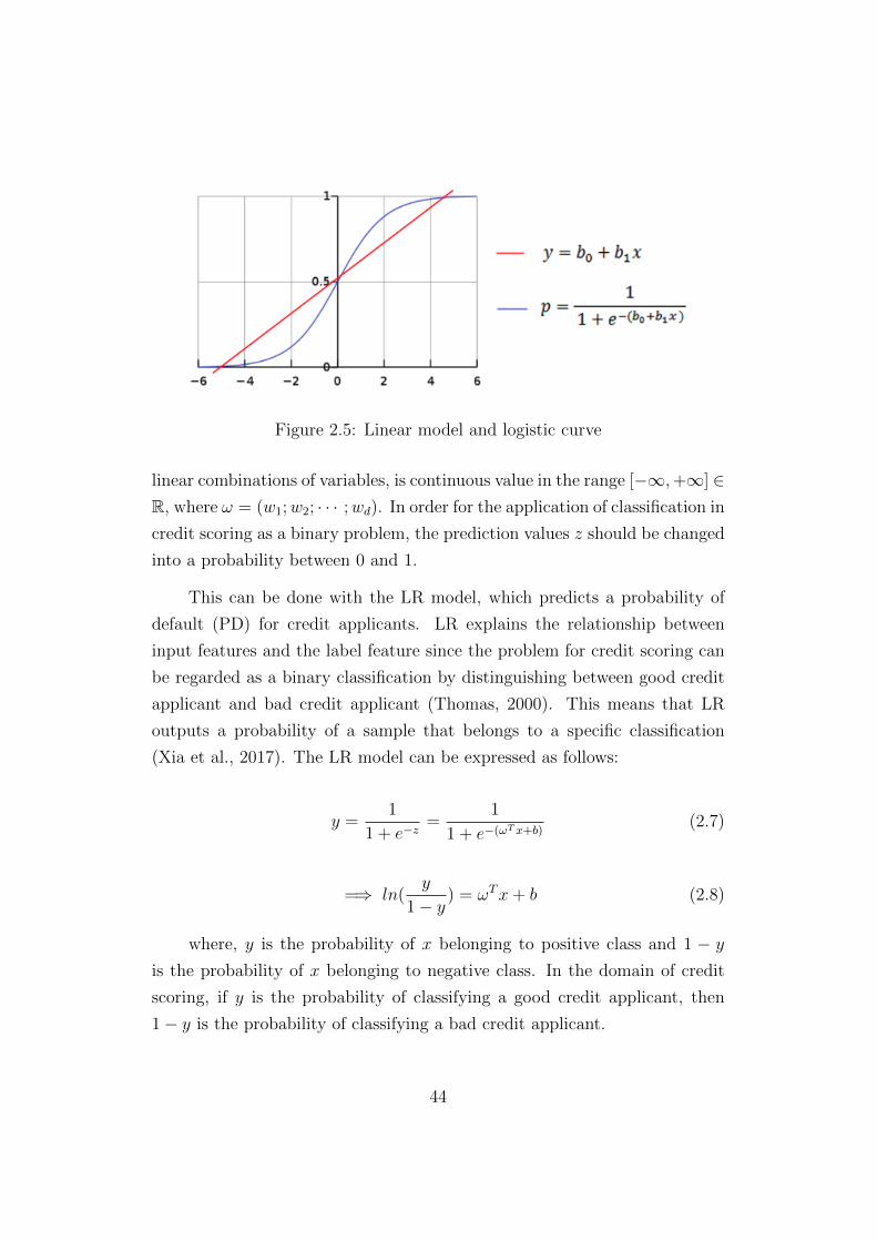
Figure 2.5: Linear model and logistic curve
linear combinations of variables, is continuous value in the range [−∞,+∞] ∈R, where ω = (w1;w2; · · · ;wd). In order for the application of classification in
credit scoring as a binary problem, the prediction values z should be changed
into a probability between 0 and 1.
This can be done with the LR model, which predicts a probability of
default (PD) for credit applicants. LR explains the relationship between
input features and the label feature since the problem for credit scoring can
be regarded as a binary classification by distinguishing between good credit
applicant and bad credit applicant (Thomas, 2000). This means that LR
outputs a probability of a sample that belongs to a specific classification
(Xia et al., 2017). The LR model can be expressed as follows:
y =1
1 + e−z=
1
1 + e−(ωT x+b)(2.7)
=⇒ ln(y
1 − y) = ωTx + b (2.8)
where, y is the probability of x belonging to positive class and 1 − y
is the probability of x belonging to negative class. In the domain of credit
scoring, if y is the probability of classifying a good credit applicant, then
1 − y is the probability of classifying a bad credit applicant.
44

y
1 − yis called as the odds, which means the ratio of the probability
that x belongs to positive class relative to the probability that x belongs to
negative class. If log is taken in odds, it can be changed as follows:
ln(y
1 − y) (2.9)
This is called as log odds or logit. This transformation shows that the
prediction value of linear regression can be approximated to log odds of the
input variables. This means that logit transformation is used for a link that
the probability of the class relates to a linear function of input attributes
(Worth and Cronin, 2003). Logit transformation can be analysed as having
strong points as follows:
• It is not necessary to make assumption on the distribution of sample
dataset and the prediction model for the probability of classification
can be made directly by sample dataset. This helps to escape from
a possible problem caused by wrong assumption of the distribution of
sample dataset.
• LR is used for not only predicting the class label but also predicting
the approximate probability. This helps the cases where the decision
making process should be done based on the probability.
For example, the good credit applicant and bad credit applicant in the
domain of credit scoring can be defined using LR model as follows:
P (y = 0 | x) =1
1 + e−(ωT x+b)(2.10)
and
P (y = 1 | x) = 1 − P (y = 0 | x) =e(ω
T x+b)
1 + e(ωT x+b)(2.11)
where x ∈ Rn represents the feature vector of credit applicant, P (y =
0 | x) is the probability of classifying x as a good credit applicant, and
45

P (y = 1 | x) is the probability of classifying x as a bad credit applicant. The
coefficients (ω and b) for parameters of model can be derived using maximum
likelihood method on a training set (Myung, 2003).
As shown in Eq. 2.8, LR model is built with the linear relationship
between logit and independent variables. The linear characteristic of LDA
and LR can be applied to develop the parametric model when the data is
linear (Akkoc, 2012; Thomas, 2000; West, 2000). Consequently, this means
that the predictive performance of LR might decrease as similar to LDA if
the data is non-linear (Ong et al., 2005).
Nevertheless, LR model has commonly been used and regarded as the
standard in the domain of credit scoring until now since it is simple and
interpretable in satisfying the explainability for credit scoring (Lessmann
et al., 2015).
2.3.3 Decision Tree
A decision tree (DT) is built with a hierarchical structure of flow that begins
from a root node, proceeds to internal nodes through each decision, and ends
at the terminal node (Bazarbash, 2019). This process is termed a recursive
partitioning (Hand and Henley, 1997). The terminal node shows the final
decision or prediction. DT can be used for both regression and classification
models, which is called as Classification And Regression Tree (CART). For
the classification, DT splits the dataset recursively based on information
(Quinlan, 1986). In other words, the selection to split at each node is decided
to maximise the purity, which is a measure of information. The other measure
of information can be impurity, Gini (Breiman et al., 1984) and Entropy
(Quinlan, 1986). DT is a non-parametric method to analyse outcome based
on the information of input (Lee et al., 2006).
In the DT model of ML, the size of the tree needs to be controlled
in order to avoid overfitting. When DT is built, the part of the tree with
redundant and less predictive power can be pruned since this pruning process
46

Figure 2.6: A hypothetical example of DT model in credit scoring
can reduce the complexity of the tree. Consequently, this leads to improve
the accuracy by reducing the overfitting (Mansour, 1997). For example, the
maximum depth of the tree and the minimum number of samples remaining
in the final nodes can be managed and optimised by hyperparameters tuning
in models.
DT has the advantages that it is easy to be interpreted and illustrated as
the flow of the decision making process for communication (Bazarbash, 2019),
as shown in Figure 2.6. Since the process of decision by the model is similar
to the process of decision by practitioners, DT can offer clear explanation
and illustration to credit applicants. The DT model in the domain of credit
scoring was first suggested by Makowski (1985).
However, DT has the disadvantages that it has not commonly been used
in practice for the modelling process, especially in FinTech. The disadvan-
tages are as follows (Bazarbash, 2019):
• DT models are easily to be overfitted in the training process and, there-
47

fore, the models cannot output the generalised prediction.
• If the dataset has high dimensionality, “curse of dimensionality” hap-
pens and DT models output a local optimal solution, not a global
optimal solution. This means that DT models can be sensitive to the
noise in the dataset, and consequently, can be unstable.
• DT models tend to be biased easily when the dataset shows strong class
imbalance, which is a common issue in credit scoring datasets.
To impede the restriction and overcome the limitation of the DT model,
DT has been extended to the ensemble learning approaches. With ensemble
learning, the variance or bias can be reduced and the prediction can be
improved. Random Forest (RF) and Gradient Boosting (GB) models are
two main DT-based ensemble methods (Bazarbash, 2019).
2.3.4 Ensemble Models
Ensemble learning algorithms combine multiple classifiers that operate dif-
ferent hypotheses in order to model one optimal hypothesis, enhancing the
performance of the model (Nascimento et al., 2014). Since datasets obtained
from different sources have their own characteristics in terms of size, form
and the label features, a single ML algorithm as the standard, i.e., LR, is not
able to model all credit scoring datasets (Xia et al., 2017). Furthermore, the
“no free lunch theorem” by Wolpert and Macready (1997) supports that a
single complex classifier is not a perfect solution for modelling credit scoring.
Recently, the ensemble approaches have been improved and they have
shown the robustness to perform the classification for accurate credit scoring.
Nanni and Lumini (2009) presented the comparative results by ensemble
approach for credit scoring. In addition, Lessmann et al. (2015) showed
that ensemble methods outperform the single ML algorithm and statistical
approaches in the domain of credit scoring. These results of recent studies
encourage further research of its effectiveness and robustness.
48

Figure 2.7: The structure of parallel and sequential ensemble
Ensemble methods can be grouped into two ways according to their
structures, which are parallel and sequential ensembles (Duin and Tax, 2000)
as shown in Figure 2.7. In parallel ensemble, the different learning algorithms
are combined with parallel structure, and each algorithm generates the mod-
els and output predictions independently. Then, final prediction is confirmed
by ensemble strategy, e.g. the majority voting. On the other hand, the differ-
ent learning algorithms in sequential structure are connected consecutively,
and each algorithm corrects the previous models. Then, the final algorithm
outputs the updated final prediction. The parallel methods such as bag-
ging (Breiman, 1996) and RF, have a weak relationship between individual
learners, while, on the other hand, the sequential methods such as boost-
ing (Schapire, 1990) and GB, have relatively a strong relationship between
individual learners.
There have been popular ensemble approaches in the literature of credit
scoring: parallel method using random forest (RF) (Yeh et al., 2012), bag-
ging (Paleologo et al., 2010; Wang et al., 2012), multiple classifier systems
(Ala’raj and Abbod, 2016a; Finlay, 2011), and sequential method using gradi-
ent boosting (GB) (Brown and Mues, 2012) and boosting (Dietterich, 2000).
49

Figure 2.8: The structure of random forest
According to Bazarbash (2019), RF and GB are the two most commonly
used ML algorithms in the domain of credit risk modelling. Furthermore,
Brown and Mues (2012) proved that RF and GB perform well for credit
scoring due to their non-parametric characteristics when compared to other
ML algorithms.
Random Forest (RF)
RF is a non-parametric tree-based ensemble model. Suggested by Breiman
(2001) and also known as forest of randomised trees, it performs the bagging
50

algorithm by searching random subspace. To produce subsets from the origi-
nal training set, the bootstrapped sampling is used. Then, several unrelated
DTs as the base learners in parallel structure are trained in these subsets,
which is termed forest. After DTs have been trained in the forest, every tree
classifies the input samples and the majority voting as ensemble strategy is
performed to determine the final prediction (Xia et al., 2018). Figure 2.8
shows the process of RF. RF has the strengths as follows (He et al., 2018):
• RF can process high dimensionality in dataset without feature selec-
tion due to decorrelation stage (Biau, 2012). Compared to DT, RF
are relatively less prone to be overfitted and have comparatively more
robust generalised prediction than DT.
• RF can show each feature importance.
• RF has high speed for training and low computational cost in parallel
structure.
Since RF takes these advantages, it has been widely applied in the real-
world areas of medicine, finance and commerce (Bazarbash, 2019). Thus, it
is also beneficial for modelling a credit scoring dataset.
However, RF is not easy to interpret the prediction, especially when
the number of randomised trees or features in samples is large. Although
feature importance, which ranks the contribution of features for final predic-
tion, can be obtained, it only shows the importance of each feature globally
across entire samples, not a certain sample. Nevertheless, the features with
importance in making predictions could be identified by the rank of features
in the models (Bazarbash, 2019). Therefore, the results of credit scoring can
be analysed and evaluated by feature importance of RF.
Gradient Boosting Decision Tree (GBDT)
GBDT, in short GB, is also a non-parametric tree-based ensemble model.
Proposed by Friedman (2001), it combines a series of weak base classifiers
51

into one strong model and enhances the classification performance. The
weak base classifier, which is generally and commonly independent DT with
a few branches, refers to a model that performs better slightly than a random
prediction (Xia et al., 2017).
Compared to the bagging algorithms that model the base learners in
parallel structure, GB performs boosting algorithms in sequential structure
of base learners. Boosting algorithms enable the additive base classifiers to
correct the errors and mistakes, and minimise the loss function consecutively
until the update becomes limited, where the loss function evaluates how well
the model fits the dataset (Xia et al., 2017).
DTs as the base learners are employed with GB in this thesis. The
performance of GB is improved by minimising the loss function and updating
the errors sequentially in previous trees. The final prediction is the sum of
predictions weighted by all previous trees (Bazarbash, 2019). Similarly, GB
allows to rank the contribution of features for final prediction by feature
importance globally on entire samples.
Given a dataset D (xk, yk)nk=1
with n samples, where x represents a set of feature vector and y denotes
the corresponding response vector, suppose that there exists the optimal
function F ∗(x) that maps feature vector x to the response vector y such that
the loss function Ψ(y, F (x)) can be minimised as follows:
F ∗(x) = argmin Ψ(y, F (x)) (2.12)
where F ∗(x) ∈ F (x). Suggested by Friedman (2001), F ∗(x) is estimated
by greedy function approximation of GB in an additive form: GB is updated
sequentially by taking the sum of previous base learners as follows:
F ∗(x) =K∑k=0
fk(x) =K∑k=0
βkh(x; θk) (2.13)
52

where f0(x) is an initial base learner and fk(x) is the k-th base learner
in k-th boost for the boosts k=1, 2, · · · , K. The optimal k-th base learner
fk(x) can be parameterised with the function βkh(x; θk), where βk represents
the optimal coefficient and θk denotes the optimal parameter for base learner.
Therefore, optimal function F ∗(x) can be obtained by those parameters
βk and θk using Eq. 2.12 and Eq. 2.13. This can be expressed as follows:
(βk, θk) = argmin
n∑i=1
Ψ(yi, Fk−1(xi) + βh(xi; θ)) (2.14)
Finally, using Eq. 2.13 and Eq. 2.14, Fk(x) can be expressed as follows:
Fk(x) = Fk−1(x) + βkh(x; θk) (2.15)
The idea of greedy function approximation by Friedman (2001) is that
the optimal βk and θk can be searched to construct the optimal base learner,
and then optimal function F ∗(x) can be approximated with the addictive
form of these constructed base learners.
Extreme Gradient Boosting (XGB)
Chen and Guestrin (2016) suggested XGB, which is an advanced version of
GB, in order to optimise the loss function and estimation of GB.
Given a dataset D (xk, yk)nk=1
with n samples and m features, where x represents a set of feature
vectors and y denotes the corresponding response vector, suppose that there
exists the optimal function F ∗(x) that maps feature vector x to the response
vector y such that the loss function Ψ(y, F (x)) can be minimised. By similar
concepts and ways with GB, F ∗(x) is estimated by function approximation
in an additive form as follows:
53
FK(x) =K∑k=1
fk(x) (2.16)
where Fk(x) represents the k-th prediction in the boosts k=1, 2, · · · ,K.
XGB uses Taylor’s expansion to approximate the loss function quickly
and employs a regularised term to manage the complexity of the tree as
learners (Xia et al., 2018) as follows:
LK(F (xi)) =n∑
i=1
Ψ(yi, FK(xi)) +K∑k=1
Ω(fk) (2.17)
where FK(xi) represents the i-th sample’s prediction on k-th boost, and
Ω(f) = γ T + 0.5 × λ ∥ ω ∥2 as regularisation term. γ is the parameter for
complexity, λ is a fixed coefficient, and ∥ ω ∥2 is the L2 norm for leaf weights
(Xia et al., 2017).
2.3.5 Neural Network
Neural network (NN) has successfully been applied in the area of natural
language process, computer vision and image, etc. The NN model has been
used to improve classification performance since it has a strong predictive
performance. Based on the motivation by the functioning of biological neuron
(Jain et al., 1996), NN is built in a similar structure to the human brain in
order to learn non-linear and complex patterns between features and output
through inner layers. (Bhattacharyya and Maulik, 2013).
Figure 2.9 shows an example of the structure of NN. Features xi =
x1, · · · , x44i=1 are employed to calculate the values of nodes zi = z1, · · · , z55i=1
in the first hidden layer. Then, nodes zi = z1, · · · , z55i=1 are used as in-
puts to evaluate the nodes in the next hidden layer. The evaluated values
obtained by sigmoid function σ(x) =1
1 + e−xare the form of weighted sum
54

Figure 2.9: The structure of neural network with four inputs (features)
x1, x2, x3, x4, two outputs y1, y2, and n hidden layers
of inputs and are in the range [0, 1] ∈ R. The sigmoid function is termed the
activation function in the architecture of NN. It is a one of the activation
functions which include softmax, hyperbolic tangent, and rectifier function
(Bazarbash, 2019).
In the case of Figure 2.9, the node z1 can be calculated as follows:
z1 =1
1 + e−(w1x1+w2x2+w3x3+w4x4+b)(2.18)
where weights w1, w2, w3, and w4 can be estimated by the contribution
of each feature x1, x2, x3, and x4 to the node z1 and the constant b is used to
adjust the bias.
Since Eq. 2.18 is similar to the form of LR, NN can be regarded as
the combinations of numerous LR where the outputs of previous layer are
employed as the inputs of the next layers (Bazarbash, 2019). Five coefficients,
w1, w2, w3, w4 and b, need to be calculated for evaluating one z in the first
layer. Since there are five nodes, z1, z2, z3, z4 and z5, in the first hidden layer,
55

25 parameters need to be estimated. This means that the more the number
of layers are in the NN, the number of parameters increases exponentially.
In the domain of credit scoring, NN has been used to improve the pre-
dictive performance as an alternative to the LR model (Angelini et al., 2008;
Atiya, 2001). As an example of Figure 2.9, suppose that the credit applicant
x has four features, x1, x2, x3, and x4. These four inputs are sent to each five
nodes z in the first layer. The weights for the five nodes z are evaluated,
and the values are accordingly processed to the activation function. Then,
the results are served as the inputs in the next layer. This process proceeds
until the final layer leads to a final prediction.
Deep NN, which is commonly called as deep learning, is the extended
version of NN having a number of hidden layers. To train deep NN models, it
is, hence, required to have more optimal architecture and high computational
power (Bazarbash, 2019).
The NN model has the main advantage that it is flexible regardless of the
assumption and characteristic of the data distribution, and is able to capture
complicated, complex and non-linear patterns in the data. This means that
NN has superior ability to capture deeper relational characteristics between
features and the output (He et al., 2020).
However, NN is a black box model in which the extracted patterns are
not comprehensible and interpretable by human beings (He et al., 2020). Due
to the lack of explainability, the NN model is not able to justify the prediction
for a credit applicant that is classified as either good credit or bad credit.
Furthermore, financial institutions are required to report the transparency in
the process of credit scoring to both regulators and credit applicants under
the Basel Accord, as discussed earlier. Therefore, interpretability is a major
drawback of the NN model. In addition, Hamori et al. (2018) argued that the
performance of deep learning models depends on the architecture of models
such as the number of hidden layers and the kind of activation function.
They showed that the ensemble approaches such as bagging and boosting
performed better than deep NN on ‘Default of Credit card clients (DC)’
56

dataset (which dataset will be discussed in Chapter 3 and Chapter 6).
Nevertheless, NN has been employed in financial application such as
daily stock return (Yeh et al., 2015), credit card fraud detection (Fu et al.,
2016), mortgage risk management (Sirignano et al., 2016), and credit risk
management (Neagoe et al., 2018) since NN shows the superior predictive
performance. It has been shown in studies that NN outperformed the para-
metric statistical LDA and LR in terms of predictive performance (Abdou
et al., 2008; Lee and Chen, 2005; West, 2000).
57

Chapter 3
Credit Scoring
This chapter expands the concepts of credit scoring to machine learning ap-
proaches in Section 3.1 and describes the process of credit scoring modelling
in Section 3.2. The three datasets which are employed in this thesis are intro-
duced and explained in Section 3.3. The process of designing credit scoring
model is summarised in Section 3.4. Following the overview of real-world
credit scoring datasets, the real-world problems of credit scoring models are
suggested in Section 3.5, Section 3.6 and Section 3.7, respectively.
3.1 Concepts
As discussed in Chapter 2, the aim of learning, i.e., machine learning, is
not to have good performance or correct assignment in training set, but to
classify labels correctly by applying the trained model to an unseen dataset.
The classification process for credit scoring proceeds to assess credit risk for
existing or new applicants in financial institutions, as to whether or not to
extend and allow the credit at a certain time. Therefore, the problem of
credit scoring is related to binary or multi-class classification and supports
the decision making process (Xia et al., 2017).
Credit risk can be defined as the risk of loss resulting from any change
58

in the applicants’ creditworthiness (Anderson, 2007). As discussed earlier, an
applicant who has good credit is likely to repay principals and interest, i.e.,
financial obligation, and this action leads to profit for financial institutions.
An applicant who has bad credit is likely to default on financial obligation
and this action leads to loss for financial institutions. In order to impede
the risk that could be occurred by the defaulters, a critical and accurate
evaluation for credit applicants should be applied to the decision making
process of classifying risk levels.
This means that credit risk could influence on non-performing financial
obligation, which is highly associated with bankruptcy and affects the sus-
tainability of financial institutions. Therefore, the risk should be managed
(Munkhdalai et al., 2019). In order to manage and minimise credit risk as
mentioned above, a data analytic approach is used for evaluating creditwor-
thiness of the applicants, which is known as credit scoring.
Hand and Henley (1997) defined credit scoring as “the term used to
describe formal statistical methods for classifying credit applicants into good
and bad risk classes”. Lyn et al. (2002) believed that the credit scoring is a
“set of decision models and their underlying techniques that aid lenders in
the granting of customer credit”. Thomas et al. (2005) suggested the aim of
credit scoring ‘to improve these decisions and make decisions consistent and
automated in credit application’.
Credit score can be modelled by using data on past applicants in order
to check the default risk of current or new applicants. In other words, finan-
cial institutions collect the data, analyse them, and make decisions whether
a credit application is accepted or rejected. This process is based on the
assumption that creditworthiness is time independent and can be deduced
from past experience or data.
The architecture of the system in the context of credit scoring is able to
derive a score or probability of default in order to assess credit risk or default
risk of the applicant. This is supported by the information on the repayment
behaviour of past borrowers as well as demographic information. As shown
59

Figure 3.1: The process of credit scoring
in Figure 3.1, the past borrowers’ data is collected and analysed in order for
new credit applicants to be classified based on the past data.
If the information about repayment behaviour is included in the dataset
and the feature which describes the repayment behaviour can be considered
as the label of default risk for new applicants, a model can be developed with
ML approaches that map the attributes of credit applicants to estimate the
label of default risk.
This system is a supervised ML model. With this characteristic, most
ML models for credit scoring are supervised models. The past data, includ-
ing repayment behaviour or delinquency information, is utilised to train the
credit scoring model (Bazarbash, 2019).
This system, finally, helps the decision making process for assigning the
applicant to the probability of risk level. Furthermore, the advancement
of data analysis as well as the enormous amount of data have enabled to
employ the ML model and make credit decisions more accurate. Therefore,
the concept and process for credit scoring meshes with the learning process of
ML as discussed in Chapter 2, and the ML modelling process can be applied
60
theoretically in the domain of credit scoring.
The set of training samples is called as training set X = x1, x2, · · · , xm,
and in the credit scoring domain X is a set of credit applicants. To make
prediction through models, the training set is composed of input data and
corresponding output information, which is termed label and denoted as
yi ∈ Y , where Y = y1, y2, · · · , ym is a label space and a set of all labels.
Similarly, Y is a set of targets for each credit applicant, which is granted
(accepted) or rejected. Therefore, the prediction for credit application is to
model a function f : X → Y which maps X to Y , with learning training set
(x1, y1), (x2, y2), · · · , (xm, ym).
In other words, after the samples as credit applicants are utilised to
develop and train the model, the trained model is able to assess the proba-
bility of default for credit application. Since the result of credit application is
credit-worthy or not, the model for credit scoring can be regarded as binary
classification.
3.2 Modelling
Credit scoring can be built by a supervised machine learning (ML) model
if the data for labelled target feature is available, and the credit scoring is
modelled by the labelled data. After the supervised learning is processed,
the classification for credit applicants as the probability of default (PD) is
performed, based on the credit scoring by modelling the relationship between
input and output features.
As discussed, the information about demographics, asset, income and
so on of credit applicants is utilised as input features in order to predict the
PD. In addition to these features, if the data has the information about the
repayment behaviour of past borrowers or delinquency and this feature can be
regarded as time independent for future credit applicants, then the ML model
can be trained with this label about the repayment behaviour or delinquency
61

Figure 3.2: The general framework for credit scoring using ML models
Table 3.1: The characteristics of the real-world credit scoring datasets used
in this studyName Source Samples Not defaulted Defaulted Num. columns* Cat. columns** Minority class (%) ∃ Missing values
GMSC Kaggle 150,000 139,974 10,026 10 0 6.68% Yes
HE Baesens et al. (2016) 5,960 4,771 1,189 10 2 19.94% Yes
DC UCI MLR 30,000 23,364 6,636 14 9 22.12% No
*Numeric columns **Categorical columns
by supervised learning (Bazarbash, 2019). Therefore, it is essential to confirm
whether or not the information about repayment behaviour or delinquency
is included in the dataset of credit scoring.
The supervised learning for credit scoring can be defined as exploring
a model f : Rn → 0, 1 or −1,+1 which maps a feature vector x ∈ Rn
to a predicted class label y ∈ 0, 1 or −1,+1. This can be expressed as
follows:
fα : x → y (3.1)
where α is the set of parameters for the model.
62
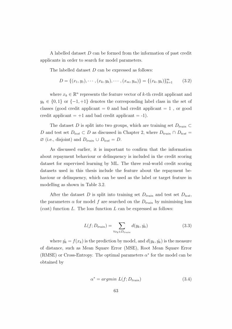
A labelled dataset D can be formed from the information of past credit
applicants in order to search for model parameters.
The labelled dataset D can be expressed as follows:
D = (x1, y1), · · · , (xk, yk), · · · , (xm, ym) = (xk, yk)mk=1 (3.2)
where xk ∈ Rn represents the feature vector of k-th credit applicant and
yk ∈ 0, 1 or −1,+1 denotes the corresponding label class in the set of
classes (good credit applicant = 0 and bad credit applicant = 1 , or good
credit applicant = +1 and bad credit applicant = -1).
The dataset D is split into two groups, which are training set Dtrain ⊂D and test set Dtest ⊂ D as discussed in Chapter 2, where Dtrain ∩ Dtest =
∅ (i.e., disjoint) and Dtrain ∪ Dtest = D.
As discussed earlier, it is important to confirm that the information
about repayment behaviour or delinquency is included in the credit scoring
dataset for supervised learning by ML. The three real-world credit scoring
datasets used in this thesis include the feature about the repayment be-
haviour or delinquency, which can be used as the label or target feature in
modelling as shown in Table 3.2.
After the dataset D is split into training set Dtrain and test set Dtest,
the parameters α for model f are searched on the Dtrain by minimising loss
(cost) function L. The loss function L can be expressed as follows:
L(f ;Dtrain) =∑
∀xk∈Dtrain
d(yk, yk) (3.3)
where yk = f(xk) is the prediction by model, and d(yk, yk) is the measure
of distance, such as Mean Square Error (MSE), Root Mean Square Error
(RMSE) or Cross-Entropy. The optimal parameters α∗ for the model can be
obtained by
α∗ = argmin L(f ;Dtrain) (3.4)
63

Then, the performance of trained model fα∗ is evaluated on the testset
Dtest with the performance measures as discussed in Chapter 2. Figure 3.2
shows the general framework for the system architecture of credit scoring
using ML.
3.3 Credit Scoring Datasets
The preconditions of three credit scoring datasets which are used to evaluate
the proposed models in Chapter 4, Chapter 5 and Chapter 6 are presented
in Section 3.3.1 and the credit scoring datasets are described specifically in
Section 3.3.2. The preprocessing methods for original datasets are suggested
in Section 3.3.3.
3.3.1 Preconditions of Datasets
The characteristics and description of the datasets used in this study are
shown in Table 3.1 and Table 3.2. The selection of these datasets is mo-
tivated by the benchmarks in the literature of credit scoring (Awan et al.,
2021; Boughaci and Alkhawaldeh, 2020; Camino et al., 2019; Engelmann
and Lessmann, 2021; Yoon et al., 2018). This choice allows to compare the
performance of our proposed models with the benchmarks and suggest the
quantitative analysis comparatively.
3.3.2 Collection of Datasets
A credit scoring dataset is composed of a group of features which can statis-
tically be analysed to be predictive in the classification of creditworthiness
(Siddiqi, 2012). Credit scoring allows the financial institutions to assess the
creditworthiness of the applicants by using a structured and tabular dataset.
Features in the credit scoring dataset describe the characteristics of the credit
applicant, including the demographics, the number of credit lines, and repay-
64

Table 3.2: The descriptions of features in GMSC, HE and DC datasetsName of feature in GMSC Description Type
SeriousDlqin2yrs Applicant experienced 90 days past due delinquency or worse Y/N (1 or 0)
RevolvingUtilizationOfUnsecuredLines Total balance on credit cards and personal lines of credit percentage
age Age of in years integer
NumberOfTime30-59DaysPastDueNotWorse Number of times applicant has been 30-59 days past due but no worse in the last 2 years. integer
DebtRatio Monthly debt payments, alimony,living costs divided by monthly gross income percentage
MonthlyIncome Monthly income real
NumberOfOpenCreditLinesAndLoans Number of Open loans (installment like car loan or mortgage) and Lines of credit integer
NumberOfTimes90DaysLate Number of times applicant has been 90 days or more past due. integer
NumberRealEstateLoansOrLines Number of mortgage and real estate loans including home equity lines of credit integer
NumberOfTime60-89DaysPastDueNotWorse Number of time applicant has been 60-89 days past due but no worse in the last 2 years. integer
NumberOfDependents Number of dependents in family excluding themselves (spouse, children etc.) integer
Name of feature in HE Description Type
BAD Applicant defaulted on loan or seriously delinquent or applicant paid loan Y/N (1 or 0)
LOAN Amount of the loan request integer
MORTDUE Amount due on existing mortgage integer
VALUE Value of current property integer
REASON DebtCon = debt consolidation; HomeImp = home improvement category
JOB Occupational categories category
YOJ Years at present job integer
DEROG Number of major derogatory reports integer
DELINQ Number of delinquent credit lines integer
CLAGE Age of oldest credit line in months real
NINQ Number of recent credit inquiries integer
CLNO Number of credit lines integer
DEBTINC Debt-to-income ratio real
Name of feature in DC Description Type
LIMIT BAL Amount of given credit in NT dollars (includes individual and family/supplementary credit) integer
SEX Gender (1=male, 2=female) category
EDUCATION (1=graduate school, 2=university, 3=high school, 4=others, 5=unknown, 6=unknown) category
MARRIAGE Marital status (1=married, 2=single, 3=others) category
AGE Age in years integer
PAY 1, PAY 2, · · · , PAY 6 Repayment status in September, August, · · · , April 2005 (categoty*(-2,-1,0, · · · , 8)) category
BILL AMT1, BILL AMT2, · · · , BILL AMT6 Amount of bill statement in September, August, · · · , April 2005 (NT dollar) integer
PAY AMT1, PAY AMT2, · · · , PAY AMT6 Amount of previous payment in September, August, · · · , April 2005 (NT dollar) integer
default.payment.next.month Default payment Y/N (1 or 0)
*-2=no consumption, -1=pay duly, 0=the use of revolving credit, 1=payment delay for one month, 2=payment delay for two months, · · · , 8=payment delay for eight
months, 9=payment delay for nine months and above
ment behaviours and so on. These features are generally a group of a set
of non-time series or non-time stamp, and ‘mutually exclusive values or a
range of non-overlapping numbers’ (Kennedy, 2013). This suggests that the
characteristics of the dataset in the domain of credit scoring include various
aspects such as the predictive power of features for classification and the
correlation and collinearity between the features. Therefore, credit scoring
datasets are commonly regarded as complex and non-linear dataset.
All credit scoring datasets used in this thesis vary in terms of the distri-
bution of samples, the number of features, and the distribution of correspond-
ing classes. For example, three datasets show moderate to strong imbalanced
class. Table 3.2 shows the detailed characteristics of credit scoring datasets.
65

In Chapter 4, ‘Give Me Some Credit (GMSC1)’ dataset is used to vali-
date the robustness of non-parametric tree-based approach with resampling
method for explainable credit scoring, focused on oversampling and model
interpretability. This proposed model is named as Non-pArameTric approach
for Explainable credit scoring (NATE) on imbalanced class.
In Chapter 5, ‘Home Equity (HE2)’ dataset is used to validate the ef-
ficacy of non-parametric tree-based oversampling technique for explainable
credit scoring, focused on non-linear and complex dataset. This approach
is cWGAN-based oversampling method paired with Stacked AutoEncoder
(SAE), named as Non-parametric Oversampling Techniques for Explainable
credit scoring (NOTE).
In Chapter 6, ‘Default of Credit card clients (DC3)’ dataset is used to
evaluate the superiority of denoising imputation techniques for credit scoring
dataset with missingness, focused on the estimation of missing values. This
approach is GAIN-based imputation method paired with randomised Sin-
gular Value Decomposition (rSVD), named as Denoising Imputation TEch-
niques (DITE) for missingness in credit scoring.
GMSC dataset is obtained from Kaggle ‘Give Me Some Credit’ competi-
tion, and HE dataset comes from a previous paper of credit scoring literature
(Baesens et al., 2016). DC dataset (Yeh and Lien, 2009) is acquired from a
previous paper of credit scoring literature and UCI Machine Learning Repos-
itory (UCI MLR) (Dua et al., 2017). The footnote provides the access to the
three datasets.
As shown in Table 3.1 and Figure 3.3, GMSC and HE datasets have
missing values in features. Missing values are common in credit scoring
datasets. The study of missing values will be discussed further in Chapter
6 using DC dataset, since DC dataset does not have missing values in fea-
tures. This allows to simulate the research of missing values and imputation
1https://www.kaggle.com/c/GiveMeSomeCredit2http://www.creditriskanalytics.net/datasets-private2.html3http://archive.ics.uci.edu/ml/datasets/default+of+credit+card+clients
66

methods in the dataset, comparing the original complete DC dataset with
the incomplete DC dataset including generated missingness.
Table 3.2 shows the descriptions of features in GMSC, HE and DC
datasets. Within the three datasets as shown in Table 3.2, bad credit samples
are defined as the cases that target features named as ‘SeriousDlqin2yrs’,
‘BAD’, ‘default.payment.next.month’, respectively, are specified as 1, which
means the applicant has defaulted on the loan or financial obligation. On
the other hand, good credit samples are classified as the cases that the label
is specified as 0, which means the applicant has paid a financial obligation
on time. These target features are binary class label as 0 or 1.
For the transformation of features, e.g., feature scaling, the range of
features in dataset affects the training process of specific models such as
Support Vector Machine (SVM) and Neural Network (NN) although non-
parametric tree-based models are rarely affected by the scale (Xia et al.,
2018). More details for data preprocessing methods are discussed in the next
section.
3.3.3 Preprocessing of Datasets
Since the quality of dataset plays a vital role as famously known as ‘Garbage
in, Garbage out’ (Beam and Kohane, 2018) in enhancing the generalised per-
formance of models, preprocessing datasets is essential for modelling credit
scoring (Garcıa et al., 2012). According to Garcıa et al. (2015), the quality
of dataset can be evaluated with three factors which are accuracy, complete-
ness and consistency, while for the real-world dataset this is not the case.
Noise, outliers and missing values in real-world datasets are generally in-
cluded. These deficiencies cause a problem in the training process of the
model since they make it difficult to extract the latent rules reflected in the
dataset (Kotsiantis et al., 2006). Therefore, preprocessing the dataset is a
crucial step prior to the modelling process and it consists of methods such
as data imputation for missing values, standardisation and normalisation
67

Figure 3.3: Missing values in features on credit scoring datasets (GMSC, HE,
and DC in order)
68

for feature scaling and feature selection and feature engineering for optimal
subset, etc.
Credit scoring datasets in the real-world have generally missing values.
This missingness might affect the modelling process or distort the analysis of
the prediction stage in the model (Jerez et al., 2010; McKnight et al., 2007).
Therefore, the missingness in the dataset needs to be handled in the stage of
data preprocessing. Substituting missing values with the estimated values in
the dataset is preferable to deleting the samples with missing values (Acuna
and Rodriguez, 2004). This imputation approaches for missingness in the
dataset will be discussed further in Chapter 6.
Figure 3.3 shows the missing values in three credit scoring datasets,
respectively. In Chapter 4 and Chapter 5, GMSC and HE datasets are pre-
processed to handle any missing values before building the model for credit
scoring. As suggested by Acuna and Rodriguez (2004), Lessmann et al.
(2015), and Ala’raj and Abbod (2016b) in the literature of credit scoring,
missing values in categorical or nominal columns are replaced with the most
frequent category in the remaining samples. In addition, missing values in
numerical columns are replaced with the mean value in the remaining sam-
ples.
On the other hand, features in the dataset have a diverse range of values.
The ML models such as Support Vector Machine (SVM) and Neural Networks
(NN) are sensitive to the range of input values. In order to reduce the
unnecessary bias and enhance the prediction performance in models, the
dataset needs to be transformed with normalisation. This rescales the range
of values in features to be in the interval [0, 1] ∈ R. The normalisation is
expressed as follows:
Normalised(Vi) =Vi −min(Vi)
max(Vi) −min(Vi)(3.5)
In this thesis, normalising the dataset is utilised in the preprocessing
stage in Chapter 5 and Chapter 6. Specifically, the HE dataset in Chapter 5
is normalised prior to the stage of Stacked AutoEncoder (SAE) for extracting
69

the latent features in a non-linear dataset since SAE is a kind of NN. The DC
dataset in Chapter 6 is normalised prior to the stage of randomised Singular
Value Decomposition (rSVD) for reducing the noise in the dataset since the
imputation approach in Chapter 6 is based on GAIN algorithms, which GAIN
is a kind of NN.
As discussed, the scale of features does not greatly affect non-parametric
tree-based models (Xia et al., 2018). This thesis mainly focuses on non-
parametric tree-based approaches for credit scoring modelling.
In order to simplify the training process of models, Feature Selection
(FS) or Feature Engineering (FE) can be applied (Falangis and Glen, 2010).
The optimal subset of the original dataset is able to improve prediction per-
formance by reducing the dimensionality of features in the dataset (Guyon
and Elisseeff, 2003). The process of FS or FE is normally applied to the
dataset after the process of substituting the missing values with estimated
values and normalising features in the dataset. The subset of original dataset
through FS or FE, hence, has the most effective and least redundant features
for training the models.
The difference between FS and FE is that FS optimises a subset of fea-
tures from all features in the dataset, while FE generates new features from
the current features (Dastile et al., 2020). Liang et al. (2015) argued that FS
does not always guarantee the performance improvement of models. In addi-
tion, Liu and Schumann (2005) also argued that “there is no economic theory
to represent which features are relevant to creditworthiness, and the process
of choosing the best subset of existing features is unsystematic and domi-
nated by arbitrary trial”. However, Bijak and Thomas (2012) and Brown
and Mues (2012) suggested that the least redundant features can improve
the performance of the credit scoring model.
SAE is a type of AutoEncoder (AE) and can be used to extract the
features for FE. AE is an unsupervised NN that is fully connected to re-
construct the representation or codings for feature extraction (Hinton and
Salakhutdinov, 2006). AE consists of encoder and decoder. Figure 3.4 shows
70

Figure 3.4: The structure of SAE
the structure of AE. In the process of encode, non-linear mapping function
f maps input x to the representation h in hidden layer. The encoding can
be expressed as follows:
h = f(ωx + b) (3.6)
where ω denotes the weight between the input x and the representation
h, and b represents the bias. ω and b can be obtained after the learning
process.
In the process of decode, x′ can be obtained by the representation h in
hidden layer. The decoding can be expressed as follows:
x′ = f ′(ω′h + b′) (3.7)
where ω′ denotes the weight between the representation h and the output
71

x′, and b′ represents the deviation. Therefore, x′ is the reconstruction as the
output.
AE is trained to minimise the loss, i.e. minimising the reconstruction
error. The loss function L can be expressed as follows:
L(x, x′) =1
N
∑xk∈Dtrain
∥ x− x′ ∥2 (3.8)
where Dtrain = (xk)Nk=1 is a training set.
The loss function L can be minimised by the iterative learning. With
this process, SAE can be used to extract latent characteristics in features
since it has the capability to deal with non-linear and complex data for
classification (Zhang et al., 2020).
For GMSC dataset in Chapter 4, three features describing the number of
late payments after due date, which are ‘NumberOfTime30-59DaysPastDueNot-
Worse, NumberOfTime60-89DaysPastDueNotWorse, NumberOfTimes90Days-
Late’ are combined into a new single feature named as ‘CombinedDefaulted’.
Then, ‘NumberOfTime60-89DaysPastDueNotWorse, NumberOfTimes90Days-
Late’ are dropped. In addition, two features presenting the number of loans,
which are ‘NumberOfOpenCreditLinesAndLoans, NumberRealEstateLoan-
sOrLines’ are merged into a new single feature named as ‘CombinedCredit-
Loans’. Then, ‘NumberOfOpenCreditLinesAndLoans, NumberRealEstateLoan-
sOrLines’ are dropped. Through this FE, the total number of features on
GMSC dataset finally changes from 10 to 8.
For HE dataset in Chapter 5, SAE is applied to the original dataset
for extracting the latent characteristics. The extracted three features, which
are named as “en1, en2, en3”, are merged into existing features. The total
number of features on HE dataset, hence, changes from 12 to 15.
72

3.4 Summary for Designing Proposed Credit
Scoring Model
The previous sections discussed the essential steps to build a credit scoring
model using ML. The proposed models in this thesis mainly follow the general
framework of system architecture shown in Figure 3.2. Therefore, all steps
can be summarised as follows:
1. Collecting the dataset
2. Preprocessing the dataset
3. Selecting the features or engineering the features
4. Developing the classifiers and modelling credit scoring
5. Evaluating the predictive performance of built credit scoring model
6. Predicting the classification and explaining the credit scoring model as
XAI
These main steps need to proceed sequentially in order to obtain the
necessary levels of effectiveness and robustness.
The conceptual and experimental system architecture of the proposed
credit scoring model was overviewed. The next sections will discuss the three
key issues of credit scoring in more details.
3.5 Explainable Models: Parametric vs Non-
parametric
LR is regarded as the industry standard for credit scoring. It is supported by
the literature of research, since it shows the acceptable level of performance
73
as well as interpretability when compared to the performance of other clas-
sifiers (He et al., 2018). As a parametric model, LR has the advantages of
explainability, interpretability, less computational cost for resource and time,
and less demand for a huge training dataset.
The parametric model can be expressed with the form of function that
connects the target feature to input features in a relational and linear way.
However, the parametric model normally does not have strong predictive
performance in a non-linear and complex dataset. It shows poor prediction
power, which is its main weakness (Bazarbash, 2019).
On the other hand, tree-based models such as RF, GB and XGB are
non-parametric models. These non-parametric models are trained on mini-
mal functional assumptions in the learning process from the dataset. This
characteristic allows to make models flexible. Therefore, tree-based models,
as non-parametric models, have high predictive performance when compared
to LR. The prediction power generally tends to increase as the number of
samples increases in training tree-based models.
In addition, Russell and Norvig (2002) emphasised that non-parametric
models are appropriate and robust in the cases where the data is sufficient
and the prior knowledge of the domain is not necessary, and the attention
for feature selection is not vital. However, tree-based models tend to be
prone to overfitting and, hence, optimal hyperparameters are necessary to
be searched by tuning in the training process. Furthermore, it is hard to
understand tree-based models and interpret the reasons for prediction.
To overcome this trade-off between the explainability and the predictive
power of parametric and non-parametric models in the domain of credit scor-
ing, non-parametric tree-based models which are combined with recent study
about explainable AI are proposed. These proposed explainable models al-
low us to analyse the prediction by SHAP (SHapley Additive exPlanations)
values in addition to high predictive performance.
In Chapter 4, this paper performs a comparative experiment between
parametric LR and non-parametric tree-based ensemble models for classifi-
74

cation based on imbalanced credit scoring dataset. In the domain of credit
scoring, the problem of class imbalance is common since most applicants
for loan have good credit and the remaining few applicants have bad credit.
Therefore, a large class imbalance is present and datasets normally show the
Imbalance Ratio (IR).
In the experiment, the robustness of non-parametric models such as RF,
GB and XGB is analysed, and whether both the standard oversampling and
undersampling techniques for imbalanced dataset could improve the perfor-
mance of classification for credit scoring, is discussed. Furthermore, hyperpa-
rameters are optimised to deal with the problem of overfitting in tree-based
models, and these tree-based models are interpreted by ‘Explainer’, as sug-
gested by Lundberg and Lee (2017).
The results from this experiment present that GB and XGB outper-
formed LR in classification performance. Furthermore, oversampling meth-
ods are superior to undersampling ways for handling the imbalanced class
problem. Finally, GB with oversampling technique performs best in the
credit scoring dataset.
3.6 Class Imbalance
In the classification problem, the machine learning model is trained, based on
the assumption that the training dataset has the same number of distribution
in each corresponding class (Japkowicz, 2000). If the number of difference
between each class is not very large, the machine learning model would not
be affected much in prediction of classification, while otherwise, the learn-
ing process in machine learning would be complicated and the accuracy for
performance is biased towards the majority class (Haixiang et al., 2017).
However, in realistic application of credit scoring, most datasets are fre-
quently imbalanced since applicants who have good credit are much greater
than applicants who have bad credit. Therefore, the trained model tends to
75

be overfitted and predict the most common class by maximising the accuracy
of overall classification (Drummond and Holte, 2005). This causes to mis-
classify the label in the classification problem. Cases where the number of
difference between each class is large in the classification problem are called
as class imbalance.
In the domain of credit scoring, the problem of class imbalance is termed
Low Default Portfolios (LDPs), where most applicants for loan have good
credit and the remaining few applicants have bad credit. That is, datasets
have a much smaller number of samples in the minority class of bad credit
applicants than in the majority class of good credit applicants. Therefore, a
large class imbalance is present and datasets normally show imbalance ratio
(Brown and Mues, 2012).
When compared to balanced datasets, imbalanced datasets normally
cause challenges in the learning process for the classification model and re-
sult in that machine learning techniques might not be able to handle the
problem of class imbalance. Therefore, this would lead to misclassification
in discriminating the creditworthiness of applicants for loan.
According to Hand and Henley (1997), financial institutions could pre-
vent a significant amount of loss if the accuracy of classification for credit
scoring techniques would be improved with only a percent. Furthermore, He
et al. (2018) emphasised that misclassifying a bad applicant as good is more
costly than misclassifying a good applicant as bad, since this would lead to
latent loss for loans.
As discussed, financial institutions evaluate the potential risk and the
creditworthiness of potential borrowers using credit scoring models. This
impedes the loss that could be incurred by defaulted credit. The profit and
loss of financial institutions thus highly depends on credit scoring models.
Recently, most financial institutions have used the state-of-the-art ma-
chine learning models for accurate credit scoring. However, imbalanced
classes, a disproportionate ratio of observations in each class, are a com-
mon issue in the machine learning classification for credit scoring. Although
76
Synthetic Minority Oversampling TEchnique (SMOTE) has been the most
widely used to oversample the minority class, its performance is still not
reaching an acceptable level as neighbouring examples which can be from
other classes are not taken into consideration. It also performs poorly when
data is high-dimensional and non-linear. When the overlapping of classes is
increased, it can introduce additional noise.
As an alternative, Generative Adversarial Networks (GAN) has recently
gained popularity. GAN generates synthetic distribution after learning orig-
inal data, which makes it capable to model complex and non-linear distri-
butions. Several recent studies based on conditional Wasserstein GAN (cW-
GAN) have shown robust performance in modelling tabular data for credit
scoring with both numerical and categorical features. A limited number of
studies, however, have been conducted on extracting latent features from
non-linear credit scoring data and the existing studies have not considered
the explainability aspect for credit scoring models.
In Chapter 5, this paper hence proposes a novel oversampling technique
named NOTE (Non-parametric Oversampling Techniques for Explainable
Credit Scoring) to overcome such limitations. NOTE consists of three main
components. First, non-parametric stacked autoencoder (NSA) extracts la-
tent features that contain non-linear features. Second, cWGAN is utilised
to oversample the minority class. Third, using the reconstructed balanced
dataset with latent features, the credit scoring classification considering the
explainable ML aspect is performed.
Our experimental results successfully demonstrated the utility of the
novel concepts used in NOTE by outperforming the state-of-the-art over-
sampling methods by improving the classification accuracies 3.8% in gradi-
ent boosting, 11.6% in decision tree and 17.1% in logistic regression. This
could also lead to a better model explainability and stability, particularly for
non-linear credit scoring datasets.
77

3.7 Missing Values
The Basel Accord has suggested that credit risk management by models using
internal data is beneficial to evaluate the risk factors of financial institutions,
namely, probability of default (PD), loss given default (LGD), exposure at
default and maturity (EAD) (Basel, 2004). Among these risk components,
internal datasets are an essential source for PD estimation (Florez-Lopez,
2010).
As discussed, financial institutions evaluate the probability of default
(PD) and the creditworthiness of potential credit borrowers using credit scor-
ing models based on internal datasets. In a real-life application of credit
scoring, however, datasets are very often incomplete or have missing values
or do not contain sufficient records for PD estimation (Carey and Hrycay,
2001; Zentralbank, 2004).
This missingness in datasets makes it difficult to design credit predic-
tion models, or it might distort analysis when classification models make a
prediction process (Jerez et al., 2010; McKnight et al., 2007). Furthermore,
a complete dataset is generally necessary to train the state-of-the-art ML
models before the process of prediction (Ruiz-Chavez et al., 2018; Smieja
et al., 2018).
Nevertheless, the problem of missing values has often been ignored, or
basic and simple methods such as removing samples with missing values or
mean imputation for missing values, have been applied to cope with incom-
plete datasets in the analysis of credit scoring (Jerez et al., 2010; National-
bank, 2004).
As such, many studies have been suggested to deal with the problem
of missing data. The approaches can be categorised into two groups, which
are deletion and imputation (or substitution). In practice, the imputation
methods are preferable to the deletion since they allow to use all available in-
formation in the dataset. Furthermore, it is regarded as the most appropriate
and valid process for dealing with incomplete dataset to replace the missing
78

values with the estimated values. As a result, the complete dataset obtained
by imputation can be used for modelling credit scoring (Nationalbank, 2004).
As an alternative to statistical imputation and conventional ML impu-
tation methods, Generative Adversarial Imputation Networks (GAIN) (Yoon
et al., 2018) as Generative Adversarial Networks (GAN)-based imputation
approach has been proposed and shown promising results to fill the missing
values in tabular dataset. GAIN was introduced to impute the missing values
using GAN architecture in an adversarial way, and it was proved to be more
robust than conventional imputation methods. Since GAN learns the char-
acteristics of original data distribution, this makes it capable to understand
complex and non-linear missing patterns of original distributions, and finally
help fill the missing data with plausible values.
With the state-of-the-art imputation method as denoising GAIN, in
Chapter 6 this paper proposes a novel imputation technique named DITE
(Denoising Imputation TEchniques) for missing values in a credit scoring
dataset. DITE consists of three main steps. First, the dataset is rescaled
by normalisation and denoised by randomised Singular Value Decomposition
(rSVD). Second, GAIN is utilised to fill in incomplete values in the dataset.
Third, using complete dataset after imputation, credit scoring classification
is performed.
Our experimental results showed that the use of the novel concepts in
DITE outperformed the state-of-the-art imputation methods by improving
the imputation performance 7.04%, 6.34 % and 13.38 % on 20%, 50% and
80% missing condition of dataset, respectively. This could finally lead to a
more accurate credit scoring model on an incomplete credit scoring dataset.
79

Chapter 4
Non-parametric Approach for
Explainable Credit Scoring on
Imbalanced Class
4.1 Introduction
If the number of differences between each class is not very large, a machine
learning model would not be affected much in prediction of classification
while, otherwise, the learning process in machine learning would be compli-
cated and the accuracy for performance would be biased towards the majority
class (Haixiang et al., 2017).
However, in realistic application of credit scoring, most datasets are
frequently imbalanced since applicants who have good credit are much greater
than applicants who have bad credit. Cases where the number of differences
between each class is large in the classification problem are known as class
imbalance. In the domain of credit scoring, the problem of class imbalance is
referred to as Low Default Portfolios (LDPs), where most applicants for loan
have good credit and the remaining few applicants have bad credit. That
is, datasets have a much smaller number of samples in the minority class of
80

bad credit applicants than in the majority class of good credit applicants.
Therefore, a large class imbalance is present and datasets normally show
imbalance ratio (Brown and Mues, 2012).
When compared to balanced datasets, imbalanced datasets normally
cause challenges in the learning process for the classification model and re-
sult in that machine learning techniques might not be able to handle the
problem of class imbalance. Therefore, this would lead to misclassification
in discriminating creditworthiness of the applicants for loan.
To address the issue of imbalanced class, resampling methods have been
proposed (Burez and Van den Poel, 2009). Synthetic Minority Oversam-
pling TEchnique (SMOTE) has been the most widely used to oversample
the minority class, since oversampling techniques enable to use all available
information, while undersampling techniques discard the part of all available
information and result in the loss of information (Zheng et al., 2020).
As mentioned earlier, LR is regarded as the industry standard for credit
scoring and is supported by the research literature since it has been showing
acceptable performance with interpretability, when compared to the perfor-
mance of other classifiers (Brown and Mues, 2012; He et al., 2018). How-
ever, it shows limited classification performance for non-linear credit scoring
dataset since it fails to capture the non-linearity. On the other hand, non-
parametric tree-based models are able to capture the non-linear relationships
between credit risk features and credit worthiness that LR fails to detect, by
exploring the relationship in the partition of samples (Bazarbash, 2019).
Many studies have also shown that non-parametric tree-based ensemble
models perform better in credit scoring, when compared to the single algo-
rithms which is a benchmark such as LR (Nanni and Lumini, 2009; Xia et al.,
2017; Xiao et al., 2016). These ensemble approaches, hence, have been draw-
ing attention and are regarded as mainstream in the application of credit
scoring (He et al., 2018).
However, non-parametric models such as tree-based algorithms are not
easy to interpret the prediction although they have high prediction power.
81

Unexplainable models as black box artificial intelligence (AI) are not appro-
priate in the area of finance (Bussmann et al., 2021). On the other hand,
parametric models such as LR have high interpretability although they have
limited predictive performance.
To resolve this trade-off between the explainability and the prediction
performance in the domain of credit scoring, the tree-based non-parametric
models which are combined with ‘TreeExplainer’ as well as ‘LinearExplainer’
are proposed. These comprehensible models allow us to analyse the predic-
tion by SHAP (SHapley Additive exPlanations) values in addition to high
predictive performance. Lundberg and Lee (2017) suggested to explain the
prediction by SHAP, which evaluates the contribution of each feature, both
globally and locally, for the prediction of models.
The aim of this chapter, hence, is to propose Non-pArameTric tree-
based ensemble models for Explainable credit scoring, named NATE, such
as random forest (RF), gradient boosting (GB) and extra gradient boosting
(XGB) for improving classification performance on imbalanced credit scoring
dataset.
The size of the dataset will be changed by sampling methods to see how
the performance of non-parametric tree-based ensemble models are affected
by various class imbalance. Especially the robustness of non-parametric tree-
based models will be analysed, and whether undersampling and oversampling
techniques for imbalanced dataset could improve the performance of classifi-
cation for credit scoring, will be discussed in a diverse range of class imbal-
ance. Furthermore, the prediction will be explained as ‘eXplainable Artificial
Intelligence (XAI)’ in order to understand the classification for credit scoring.
The key contributions of this study are as follows:
• To demonstrate the efficacy of non-parametric models on non-linear
dataset for credit scoring
• To present the standard oversampling method by SMOTE synthesising
the minority class on imbalanced dataset, compared with undersam-
82

pling method by NearMiss
• To propose the architecture of non-parametric models on non-linear
and imbalanced credit scoring datasets
• To achieve the explainability aspect for practical application in credit
scoring as XAI as well as high predictive performance of the proposed
non-parametric model
We hypothesise that the proposed NATE will not only improve the clas-
sification performance with capturing non-linearity on imbalanced dataset,
but also build a model that are explainable for the reasons of credit scoring
prediction.
The remainder of this paper is organised as follows: Section II dis-
cusses the related studies. Section III describes the proposed NATE with its
concepts. Section IV presents the results and evaluates the performance of
NATE with the comparison on parametric models using oversampling and
undersampling techniques. Finally, Section V concludes with the summarises
of the findings from this study.
4.2 Related Work
This section discusses the related studies on evolving explainable non-parametric
tree-based models for interpretability and resampling approaches for imbal-
anced class.
4.2.1 Explainability as XAI in Credit Scoring
Explainability is important in the domain of credit scoring for both financial
institutions and credit applicants. Chen et al. (2016) described the rationale
that linear discriminant analysis (LDA) and LR can capture the optimal lin-
ear combination of input features and make credit scoring models explainable
83

Figure 4.1: Comparison between LR and GB regarding the error of explana-
tion and accuracy (Lundberg et al., 2020)
for the prediction. Despite this advantage, statistical models are often lim-
ited in terms of predictive power. This has been seen as their main weakness
(Bazarbash, 2019).
Tree-based ML ensemble classifiers such as RF and GB have been the
most popular non-linear predictive models in use (Hastie et al., 2009; Lund-
berg et al., 2020). These models are applied to the areas that make pre-
dictions based on a set of input attributes and the predictions need to be
both accurate for results and explainable for reasons. In other words, accu-
racy and explainability need to be balanced in the models, e.g., the fields
of medicine and finance (Murdoch et al., 2019). Explainability means that
the ways ML classifiers utilise input features for making predictions can be
understood (Lundberg et al., 2020).
Since LR uses logistic function, its coefficient can be easily interpretable.
However, interaction between variables is ignored with using linear decision
boundary. As tree-based algorithms such as RF and GB can be trained
in complex and non-linear decision boundary, this means that tree-based
models are hard to understand the prediction (Engelmann and Lessmann,
2021). Although DT can be interpreted by decision path, construction of
multiple trees in the decision path for tree-based ensemble models makes the
84

prediction less interpretable.
Recently, a number of research have emerged and been studied in the
field of explainable AI (XAI), and one of the study by Lundberg et al. (2020)
is about the method to make tree-based models explainable for decisions
using input contribution. A related study by Lundberg and Lee prior to
Lundberg et al. (2020) suggested ‘TreeExplainer’ with SHAP (SHapley Ad-
ditive exPlanations)(Lundberg and Lee, 2017), which is a united approach
based on Shapley values of coalitional game theory. Shapley (1953) suggested
the values which correspond to the average of each contribution of the play-
ers with a pay-off concept in cooperative game theory. This Shapley values
can be applied to estimate the contribution of each input feature for each
prediction of ML models (Bussmann et al., 2021). In other words, they allow
to explain the prediction of ML models, enable the analysis of ML models
and help us understand them, regarding both how much each feature con-
tributes for target feature globally and how a certain sample is predicted by
SHAP values of features in the certain sample locally. In addition to ‘Tree-
Explainer’, Lundberg and Lee (2017) also proposed ‘LinearExplainer’ that it
allows us to analyse the prediction by LR globally and locally using the same
ways, although its coefficient can be easily interpretable as discussed above.
On the other hand, the measure of feature importance in tree-based
ensemble models is able to compute the importance of each input and explain
the reasons for prediction. However, it is limited since feature importance
shows only the importance across entire samples, not on each case for the
prediction.
Furthermore, tree-based ensemble models are more appropriate to cap-
ture the non-linearity in the dataset. According to the results by experiments
on medical datasets (Lundberg et al., 2020) and as shown in Figure 4.1, the
greater degree of non-linearity in the dataset, the greater the explanation er-
ror and accuracy error although tree-based GB shows stability. This means
that explainability as well as accuracy drops as non-linearity in the dataset
increases, since other irrelevant features are also selected for the prediction of
85

Figure 4.2: The imbalanced class on GMSC dataset, where 0 means not
defaulted (good credit) and 1 means defaulted (bad credit)
the model and the relation between target feature and training features be-
comes less explainable (Lundberg et al., 2020). This implies that tree-based
models are preferable to linear models if the accuracy is the same by each
case.
4.2.2 Ensemble Approach with Oversampling Techniques
in Credit Scoring
Many studies have tried to optimise the classification performance in the
problem of imbalanced class on credit scoring datasets. One of the approaches
to deal with imbalanced class is a resampling techniques, as discussed earlier.
Resampling techniques are to adjust the number of samples and balance the
classes on original data by reducing the number of majority or by increasing
the number of minority. Since oversampling techniques allow to use all avail-
able information, they have been extensively preferable to undersampling
methods in the studies.
86

Table 4.1: GMSC dataset
Dataset #Samples #Good #Bad Imbalance ratio #Features
GMSC 150,000 139,974 10,026 13.961 10
Chawla et al. (2002) proposed Synthetic Minority Oversampling Tech-
nique (SMOTE). This method generates new samples between the cases in
the minority class and their neighbours in the same class using local in-
formation by K-Nearest Neighbours (KNN) algorithm rather than directly
duplicates the samples in the minority class (He et al., 2018). Han et al.
(2005) suggested Borderline-SMOTE (B-SMOTE) and Hu et al. (2009) rec-
ommended Modified-SMOTE (M-SMOTE). Both B-SMOTE and M-SMOTE
are the variants of SMOTE to overcome the limitation of SMOTE and im-
prove classification performance, since the sample in minority class and its
neighbouring sample might be in the different class when SMOTE oversam-
ples the minority class.
He et al. (2008) proposed the ADAptive SYNthetic (ADASYN) sam-
pling approach for imbalanced datasets using weighted distribution in the
samples of minority class. This method allows to reduce the biased perfor-
mance towards class imbalance.
Batista et al. (2004) proposed the comparative experiments using re-
sampling methods such as oversampling and undersampling on diverse im-
balanced datasets. Their findings concluded that oversampling methods gen-
erally show more accurate results than undersampling methods regarding
AUROC. Brown and Mues (2012) suggested comparative results using di-
verse algorithms to see the effect of resampling method on imbalanced credit
scoring datasets. The results showed that RF and GB performed well com-
pared to LR on imbalanced credit scoring datasets. Marques et al. (2013)
proposed resampling techniques on imbalanced credit scoring datasets and
proved that resampling methods, especially oversampling approaches, con-
sistently improve the classification performance. On the other hand, Khosh-
goftaar et al. (2007) argued that an even distribution does not guarantee an
87

optimal performance when handling the issue of class imbalance.
Zieba et al. (2016) employed extreme gradient boosting (XGB) for bank-
ruptcy prediction on credit datasets and showed the better results against
the benchmark. Xiao et al. (2016) proposed the ensemble approach based on
supervised clustering in order to partition the samples of each class and im-
proved classification performance on credit scoring. Xia et al. (2017) utilised
XGB model with Baysian hyperparameter tuning and showed the aspect of
interpretability as well as the improvement of classification performance in
credit scoring.
These studies have shown that non-parametric tree-based ensemble ap-
proaches have been increasing to improve the performance on imbalanced
credit scoring as well as on balanced dataset. Therefore, non-parametric
tree-based ensemble models combined with ‘TreeExplainer’ can overcome the
limitation of predictive performance in LR as the standard as well as adding
interpretability for prediction in the domain of of credit scoring.
4.3 NATE: Non-pArameTric approach for Explainable
credit scoring on imbalanced class
The NATE consists of four stages, which are as follows:
1. Collecting GMSC dataset
2. Balancing the dataset to undersample the majority class (good credit
sample) by NearMiss or to oversample the minority class (bad credit
samples) by SMOTE
3. Predicting classification on both parametric models and non-parametric
models using oversampled and undersampled dataset for comparison
4. Explaining the model by ‘TreeExplainer’ and ‘LinearExplainer’ as XAI
88

These stages need to process sequentially in order to obtain the neces-
sary levels of effectiveness.
GMSC (Give Me Some Credit) dataset is used to test tree-based ensem-
ble classifiers for evaluating the performance on different imbalance ratios
against LR. The dataset shows the demographics, payment behaviour and
delinquency information for the samples and comes from Kaggle competi-
tion which is called as ‘Give me some credit’. The dataset is widely used
as the benchmark in the study of credit scoring literature (Engelmann and
Lessmann, 2021).
There are 150,000 samples in the dataset with approximately 140,000
not defaulted credit samples and 10,000 defaulted credit samples, respec-
tively. Bad credit samples are defined as the cases that target feature named
‘SeriousDlqin2yrs’ is specified as 1, which means the applicant has defaulted
on the loan. On the other hand, good credit samples are classified as the
cases that the label is specified as 0, which means the applicant has paid
a financial obligation. This is a binary class label. The dataset was used
due to its non-linearity in the results (Engelmann and Lessmann, 2021) for
validating the robustness of non-parametric models against the parametric
model.
The initial dataset shows the percentage of minority class in total as
6.684 % and Imbalance Ratio (IR) as 13.961, which is the number of the
majority class divided by the number of the minority class. The dataset
contains 10 features that can directly be interpreted into a credit scoring
system, excluding target feature. Table 4.1 shows the description of the
dataset and Figure 4.2 shows the imbalanced class in the dataset.
In order to have the different imbalance ratio or proportion in credit
samples of the dataset, the number of distribution in the dataset has been
changed to give different class distribution. This could be done by sampling
techniques that are used for changing distribution of imbalanced dataset with
under-sampling good credit samples or over-sampling bad credit samples,
since the number of good credit samples is much higher than the number of
89

Figure 4.3: The balanced class distribution by NearMiss
Table 4.2: Undersampled dataset
Undersampling #good 7%(original) 15% 32% 50%
Imbalance ratio 13.961 5 2 1
#Not defaulted 139,974 50,130 20,052 10,026
#Defaulted 10,026 10,026 10,026 10,026
bad credit samples as described above.
There are two standard techniques that have been commonly used for
dealing with imbalanced class, which are NearMiss for undersampling and
SMOTE for oversampling. Table 4.2 and 4.3 show the resampled credit
dataset with different imbalanced ratio and distributions of good credit and
bad credit, respectively.
By the method of undersampling, NearMiss suggested by Mani and
Zhang (2003), has been applied to the original dataset. NearMiss is an un-
dersampling method that eliminates the samples of majority class randomly
using the distance-based or near-neighbour method. When the samples of
majority class and the samples of minority class are neighbouring, the sam-
ples of the majority class are removed until the class distributions are bal-
anced. Figure 4.3 shows the balanced class distribution by NearMiss.
From 139,974 good credit samples, 50,130 samples have been used to
make the ratio of class imbalance as 5 and the percentage of bad credit
class in total as 15 %; 20,052 samples have been used to make the ratio of
class imbalance as 2 and the percentage of bad credit class in total as 33
%; 10,026 samples have been used to make the ratio of class imbalance as 1
90

Figure 4.4: The synthetic sample generated by SMOTE
Figure 4.5: The balanced class distribution by SMOTE
and the percentage of bad credit class in total as 50 %. NearMiss, finally,
undersampled the majority samples, which was reduced to the total number
of minority samples and the dataset has been balanced.
On the other hand, by the method of oversampling, Synthetic Minority
Oversampling Technique (SMOTE) suggested by Chawla et al. (2002) has
been applied to the original dataset. SMOTE is an oversampling method that
generates synthetic samples using local information near the samples by K-
Nearest Neighbour (KNN). After selecting a sample xi in the minority class,
neighbouring xi is determined by KNN as shown in Figure 4.4 (a). Then,
xsynthetic between existing samples of minority class is randomly generated
with λ in interval [0, 1] as shown in Figure 4.4 (b). Finally, the number of
the minority class is oversampled to the same number of the majority class
as shown in Figure 4.5. SMOTE can be expressed as follows:
xsynthetic = xi + λ(xi − xi), λ ∈ [0, 1] (4.1)
91

From 10,026 bad credit samples, 24,228 samples have been used to make
the ratio of class imbalance as 5.622 and the percentage of bad credit class
in total as 15 %; 65,797 samples have been used to make the ratio of class
imbalance as 2.064 and the percentage of bad credit class in total as 32 %;
135,867 samples have been used to make the ratio of class imbalance as 1
and the percentage of bad credit class in total as 50 %. SMOTE, finally,
oversampled the minority samples, which increased to the total number of
majority samples and the dataset has been balanced.
As a result, by resampling the class distribution, six datasets are created
from the original dataset. The performance of non-parametric tree-based
ensemble models can be evaluated and compared against the LR model on the
original dataset of the percentage of class imbalance 6.694 % and imbalance
ratio 13.961 as a benchmark.
Table 4.3: Oversampled dataset
Oversampling #bad 7%(original) 15% 32% 50%
Imbalance ratio 13.961 5.622 2.064 1
#Not defaulted 139,974 136,208 135,784 135,867
#Defaulted 10,026 24,228 65,797 135,867
Following balancing the class distribution by resampling techniques,
tree-based ensemble algorithms perform the prediction for credit scoring as
non-parametric approach.
Figure 4.6 shows the overall of system architecture. Through this ex-
periment, it can be validated whether non-parametric algorithms paired with
resampling techniques could improve the performance of classification in the
cases where datasets show class imbalance, against the standard method as
LR on original imbalanced dataset.
ML classifiers including tree-based models are employed for performance
comparison and they are as follows:
Logistic Regression (LR) has been a commonly used model in the do-
92

main of credit scoring since it is easily interpretable (Cox, 1958). Linear
Discriminant Analysis (LDA) is a statistical learning method to model a lin-
ear combination of features that separates the class (Fisher, 1936). Both
LR and LDA are the parametric models. K-Nearest Neighbour (KNN) is
a distance-based classifier to calculate the distance between input feature
vectors and assign the points to the class of its K-nearest neighbours (Hen-
ley and Hand, 1996). KNN is a non-parametric algorithm. Decision Tree
(DT) splits the dataset recursively based on information for the classifica-
tion (Quinlan, 1986) and is a non-parametric model. Naive Bayes (NB) is a
probabilistic classifier based on Bayesian theorem (Rish et al., 2001). NB is
commonly regarded as parametric model although it can be either paramet-
ric or non-parametric depending on the combination of parameters. Random
Forest (RF) is an ensemble method aggregated with multiple decision tree
classifiers (Breiman, 2001). Gradient Boosting (GB) is a boosting method to
combine weak classifiers into one strong model and enhance the classification
performance (Friedman, 2001). DT as base learner is used in the experi-
ment of GB in this study. Both RF and GB are non-parametric models.
Extreme Gradient Boosting (XGB) is non-parametric model that combines
with tree-models of GB to classify different tasks and optimise them (Chen
and Guestrin, 2016).
The performance measure of this experiment is the Area Under the
Receiver Operator Characteristic curve (AUROC) as discussed in Chapter
2. As the accuracy of classification performance in imbalanced dataset tends
to be biased towards the majority class as discussed earlier, the measure of
performance as AUROC is used, which is the standard metric for evaluating
classification for imbalanced dataset (Haixiang et al., 2017; Huang and Ling,
2005).
Following performing the prediction by ML models, the prediction can
be interpreted by explanation with ‘TreeExplainer’ and ‘LinearExplainer’.
As discussed, SHAP suggested by Lundberg and Lee (2017) allows to
explain the prediction of a certain sample by estimating the contribution of
93

Figure 4.6: The system architecture
each feature. Both ‘TreeExplainer’ as the estimation for tree-based models
and ‘LinearExplainer’ as the estimation for LR model can be applied to
interpret ML models. SHAP can be represented by an additive form of
feature attribution with Shapley values (Shapley, 1953) as follows:
g(z′) = ϕ0 +M∑i=1
ϕiz′i (4.2)
where g is the model for explanation, i.e., the approximation of the
prediction, z′ ∈ 0, 1M is the coalitional vector (or called as ‘simplified
features’ in the study of Lundberg and Lee (2017)), describing 1 as ‘present’
and 0 as ‘absent’, M is the maximum of coalitional size, i.e., the number of
the employed input features, and ϕi ∈ R is the attribution for feature i.
For example, if the values for all features are present (z′ = 1), then Eq.
4.2 can be simplified as follows:
94
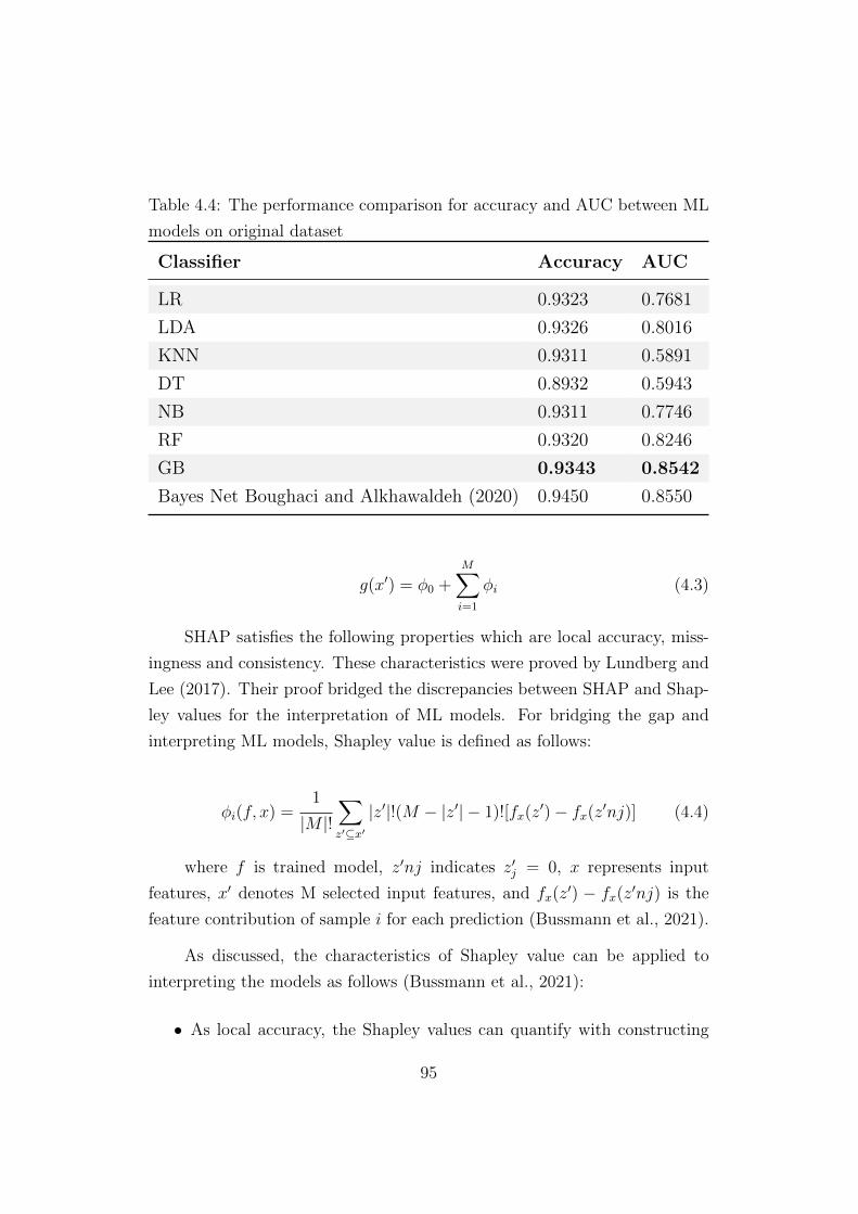
Table 4.4: The performance comparison for accuracy and AUC between ML
models on original dataset
Classifier Accuracy AUC
LR 0.9323 0.7681
LDA 0.9326 0.8016
KNN 0.9311 0.5891
DT 0.8932 0.5943
NB 0.9311 0.7746
RF 0.9320 0.8246
GB 0.9343 0.8542
Bayes Net Boughaci and Alkhawaldeh (2020) 0.9450 0.8550
g(x′) = ϕ0 +M∑i=1
ϕi (4.3)
SHAP satisfies the following properties which are local accuracy, miss-
ingness and consistency. These characteristics were proved by Lundberg and
Lee (2017). Their proof bridged the discrepancies between SHAP and Shap-
ley values for the interpretation of ML models. For bridging the gap and
interpreting ML models, Shapley value is defined as follows:
ϕi(f, x) =1
|M |!∑z′⊆x′
|z′|!(M − |z′| − 1)![fx(z′) − fx(z′nj)] (4.4)
where f is trained model, z′nj indicates z′j = 0, x represents input
features, x′ denotes M selected input features, and fx(z′) − fx(z′nj) is the
feature contribution of sample i for each prediction (Bussmann et al., 2021).
As discussed, the characteristics of Shapley value can be applied to
interpreting the models as follows (Bussmann et al., 2021):
• As local accuracy, the Shapley values can quantify with constructing
95

Figure 4.7: The performance comparison for accuracy and AUC between ML
models on original dataset
an explainable model that estimates the original model by an additive
form locally for a certain sample x.
• As missingness, if a feature is 0 (i.e., a feature is missing), then the
Shapley value is 0 (i.e., a missing feature has zero attribution).
• As consistency, if the contribution of feature increases or decreases
regardless of other features in the model, then Shapley value also in-
creases or decreases.
With these characteristics, the Shapley values of the features are cal-
96

Figure 4.8: The performance comparison for accuracy (above) and AUC
(below) between ML models on original dataset
culated by SHAP (Lundberg et al., 2020) for the explanation of predictions
both locally and globally in credit scoring models.
On the other hand, Local Interpretable Model-agnostic Explanations
(LIME) also allows to explain the prediction by building sparse linear models
in the ML models. This means that LIME is able to explain how ML models
work around the prediction by using local linearity. However, LIME lacks
the local accuracy and consistency for the interpretation of models, whilst
SHAP suggests the guarantee of the characteristics, according to Lundberg
and Lee (2017). In addition to this lack of properties, there is no theoretical
97

basis why the prediction of ML models can be interpreted by using local
linearity around the prediction, whilst SHAP is supported by mathematical
proof as discussed earlier.
Furthermore, the primary models in the proposed NATE are non-parametric
tree-based models. SHAP is based on the tree-based models and allows intu-
itively to visualise the explanation both locally and globally when compared
to LIME. Therefore, SHAP supported by theoretical proof and intuitive vi-
sualisation is more appropriate to the explainable aspect of the prediction
than LIME.
As shown in Figure 4.6, the overall system architecture for the proposed
study is summarised as follows:
Firstly, credit scoring dataset is pre-processed. In this stage, features are
transformed by methods such as standardisation and normalisation. Miss-
ing values in features are handled. Secondly, feature extraction techniques
such as feature engineering are applied to datasets, as discussed in Section
3.3.3. During this process, the importance of features is calculated, subsets
of features are optimised, model-based features are selected, and imbalanced
datasets are resampled to certain ratio or balanced class, in order to decide
the most effective and least redundant features or subsets before training ML
models.
The ensemble classifiers such as RF, GB and XGB are employed to train
the model and perform the classification with datasets of different imbalance
ratio that are resampled by sampling techniques, in order to validate how
class imbalance or imbalance ratio affects tree-based ensemble classifiers in
the domain of credit scoring.
The results of performance for non-parametric models such as RF, GB
and XGB are compared between the results of performance for parametric
models such as LR as a benchmark which is the most frequently used classifier
in the domain of credit scoring, as discussed.
Finally, the interpretation by ‘Explainer’ is performed to understand
98

Table 4.5: The performance comparison of AUC on different IR of dataset
Undersampling #good 7%(original) 15% 32% 50%
Imbalance ratio (IR) 13.961 5 2 1
#Not defaulted 139,974 50,130 20,052 10,026
#Defaulted 10,026 10,026 10,026 10,026
LR 0.7726 0.7916 0.8112 0.8272
RF 0.8489 0.8576 0.8744 0.8848
GB 0.8561 0.8609 0.9156 0.9369
XGB 0.8542 0.8581 0.9071 0.9274
Bayes Net Boughaci and Alkhawaldeh (2020) 0.8550 N/A N/A N/A
Oversampling #bad 7%(original) 15% 32% 50%
Imbalance ratio (IR) 13.961 5.622 2.064 1
#Not defaulted 139,974 136,208 135,784 135,867
#Defaulted 10,026 24,228 65,797 135,867
LR 0.7726 0.8385 0.8342 0.8361
RF 0.8489 0.9299 0.9465 0.9561
GB 0.8561 0.9510 0.9708 0.9808
XGB 0.8542 0.9485 0.9657 0.9757
Bayes Net Boughaci and Alkhawaldeh (2020) 0.8550 N/A N/A N/A
the contributions of input features for the prediction of credit scoring both
locally and globally.
4.4 Results
This section evaluates classification performance by resampling and inter-
prets the prediction by Explainer.
4.4.1 Benchmarks on the Original Dataset
Table 4.4 and Figure 4.7 show the performance comparison of accuracy and
AUC on both parametric and non-parametric classifiers on original imbal-
anced credit scoring dataset. The accuracy and AUC for performance mea-
99

Table 4.6: Searching space for hyperparameters in Table 4.5
Algorithm Hyperparameter Value
LR penalty ‘none’, ‘L1’, ‘L2’, ‘elasticnet’inverse penalty coefficient C loguniform(1e-5, 100)
solver ‘newton-cg’, ‘lbfgs’, ‘liblinear’
RF n estimators [100, 1000]
max features ‘auto’, ‘sqrt’max depth [1, 20]
min samples split 1, 2, 5, 10min samples leaf 1, 2, 4, 8bootstrap ‘True’, ‘False’
GB n estimators [100, 1000]
learning rate ‘0.01’, ‘0.1’, ‘0.5’max depth [1, 20]
Base learner Decision Tree
XGB n estimators [100, 1000]
learning rate ‘0.01’, ‘0.1’, ‘0.5’max depth [1, 20]
Base learner Decision Tree
sure are calculated by 10-fold cross validation. Since the number of samples
in each class has a huge difference, i.e., the dataset is heavily imbalanced, the
accuracy is biased towards the majority class as shown in Table 4.4. This
implies that the accuracy is not a proper measure for evaluating the perfor-
mance. Therefore, AUC as another metric is considered at the same time,
as discussed earlier.
As shown in Table 4.4, Figure 4.7 and Figure 4.8, GB has the highest
accuracy and AUC. When compared to parametric algorithms such as LR,
LDA and NB, non-parametric ensembles classifiers such as RF, GB, and
XGB show better results aligned with the previous studies in both accuracy
and AUC. It is proved that RF,GB, and XGB as non-parametric models
100

Figure 4.9: AUC improvement of classification models by undersampling
method (NearMiss) against LR on original dataset (IR=13.9)
have the ability to focus on local features in imbalanced dataset and non-
linear dataset (Brown and Mues, 2012). Therefore, non-parametric models
need to be explored further regarding classification performance, based on
the justification of these results.
4.4.2 Performance Comparison on Resampled Dataset
The performance of classifiers on varying imbalance ratio between the classes
is compared on seven datasets including the original dataset in order to
validate the effect of imbalanced dataset.
In order for the performance comparison between parametric and non-
parametric models, 70% of the dataset is used to train the models and the
remaining 30% of the dataset is used to test the models for evaluating the
performance by AUC. In addition, tree-based models with non-pruning have
the risk of overfitting on the dataset. Hyperparameters of LR, RF, GB and
XGB, hence, are optimised by random search with 3-fold cross validation
over searching space on balanced dataset (IR=1), in order to have optimal
performance. Table 4.6 shows the searching space for hyperparameters.
101

Figure 4.10: AUC improvement of classification models by oversampling
method (SMOTE) against LR on original dataset (IR=13.9)
Table 4.5 shows the AUC comparison of tree-based ensemble classifiers
against LR as a benchmark on the different IR by undersampling and over-
sampling techniques. Figure 4.9 and Figure 4.10 show the AUC improvement
by NearMiss and SMOTE, respectively. As shown in Table 4.5, Figure 4.9
and Figure 4.10, most classifiers perform better on lower imbalance ratio by
both undersampling NearMiss and oversampling SMOTE, which means the
more similar the number of class distributions are, the better performance
we can expect. It is proved that resampling methods are robust in imbal-
anced dataset, and especially SMOTE as oversampling method improved the
performance further than NearMiss as undersampling approach.
Furthermore, non-parametric models such as RF, GB and XGB have
better results against LR as the benchmark on both original imbalanced and
resampled balanced dataset as shown in Table 4.5. This means that non-
parametric models can capture the non-linearity if the dataset is complex
and non-linear. Therefore, the efficacy of non-parametric models on non-
linear credit scoring datasets is demonstrated.
In addition, Engelmann and Lessmann (2021) proved that oversampling
technique in non-linear dataset showed the best classification performance
102

Figure 4.11: The ROC of non-parametric classifier against parametric model
on original dataset (above) and balanced dataset (below)
when paired with tree-based models like RF, GB and XGB. Therefore, Table
4.5 supports their results by Engelmann and Lessmann (2021) since GMSC
dataset is non-linear credit scoring dataset, and the standard oversampling
method paired with tree-based models is suggested on imbalanced non-linear
datasets.
As shown in Table 4.5, Figure 4.8, Figure 4.9 and Figure 4.10, GB has
the best results on all imbalance ratios on imbalanced datasets as well as on
the balanced dataset by both undersampling and oversampling methods.
103
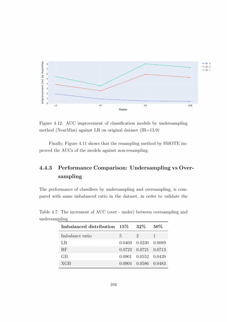
Figure 4.12: AUC improvement of classification models by undersampling
method (NearMiss) against LR on original dataset (IR=13.9)
Finally, Figure 4.11 shows that the resampling method by SMOTE im-
proved the AUCs of the models against non-resampling.
4.4.3 Performance Comparison: Undersampling vs Over-
sampling
The performance of classifiers by undersampling and oversampling, is com-
pared with same imbalanced ratio in the dataset, in order to validate the
Table 4.7: The increment of AUC (over - under) between oversampling and
undersampling
Imbalanced distribution 15% 32% 50%
Imbalance ratio 5 2 1
LR 0.0469 0.0230 0.0089
RF 0.0723 0.0721 0.0713
GB 0.0901 0.0552 0.0439
XGB 0.0904 0.0586 0.0483
104

Figure 4.13: AUC improvement of classification models by oversampling
method (SMOTE) against LR on original dataset (IR=13.9)
effect of resampling techniques. The difference of AUC is obtained by AUC
of oversampling minus AUC of undersampling, based on the same imbalance
ratios of resampled dataset and the different sampling methods.
As shown in Table 4.7, most classifiers perform better with oversampling
techniques since the values are positive. For example, the increments of AUC
on RF are 0.0723, 0.0721 and 0.0713 in the cases of 15%, 32% and 50% bad
credit samples in total, respectively. The increments of AUC on GB are
0.0901, 0.0552 and 0.0439 in the cases of 15%, 32% and 50% bad credit
samples in total, respectively. The increments of AUC on XGB are 0.0904,
0.0586 and 0.0483 in the case of 15%, 32% and 50% bad credit samples in
total, respectively.
As shown in Figure 4.12 and Figure 4.13, SMOTE improved AUCs
further than NearMiss in both all classifiers and imbalance ratio. Therefore,
NATE successfully suggested the architecture of non-parametric models on
non-linear and imbalanced credit scoring dataset by achieving the best AUC.
105

Figure 4.14: SHAP value plot for individual sample predicted by GB
Figure 4.15: SHAP value plot for individual sample predicted by GB
4.4.4 Interpretability of Predictions
Figure 4.14 and Figure 4.16 show the interpretation of the prediction for
credit scoring on an individual good credit applicant. It explains which
features contribute to the prediction when a certain individual sample is
classified as ‘not defaulted’, and helps us interpret the model locally. ‘Com-
binedDefaulted = 0’ and ‘NumberOfTime30-59DaysPastDueNotWorse = 0’
are two of the most important features for the prediction in non-defaulter.
More details are shown in Figure 4.14, where the base value 0.5 is
a turning point and threshold between a good and bad credit applicant.
The blue features such as ‘CombinedDefaulted = 0’ and ‘NumberOfTime30-
59DaysPastDue-NotWorse = 0’ push the sample to the left which is the
direction to the good credit, and the red features such as ‘RevolvingUti-
lizationOfUnsecuredLines=0.799’ and ‘age=34’ push the sample to the right
which is the direction to the bad credit. Through the combination of each
feature impact in the NATE, the sample is finally classified as a good credit
applicant with the value 0.22, which is below the threshold 0.5
Furthermore, NATE shows how the model classifies the applicant as a
good credit through the decision path in the process, as shown in Figure
4.16. The decision starts from ‘DebtRatio’ at the bottom, moves onto the
next features, and finishes at ‘CombinedDefaulted’, reflecting the magnitude
106

Figure 4.16: SHAP decision plot for individual sample predicted by GB
Figure 4.17: SHAP decision plot for individual sample predicted by GB
of features impact. Finally, NATE classifies this sample as a good credit
applicant, which is the left from the middle as the base value 0.5.
On the other hand, Figure 4.15 and Figure 4.17 show the interpretation
of the prediction for bad credit scoring on an individual credit applicant which
is classified as ‘defaulted’. ‘CombinedDefaulted = 1’ and ‘RevolvingUtiliza-
tionOfUnsecuredLines = 0.796’ are two of the most important features for
the prediction in the defaulter.
Therefore, Figures 4.14, 4.15, 4.16 and 4.17 show that the models can
be interpreted by Shapley values and the contribution of each feature in a
certain sample can be explained locally.
With the average of Shapley values across entire samples, the model can
107

Figure 4.18: Comparison of the average of SHAP feature importance on GB
Figure 4.19: Comparison of the aggregation of SHAP values on the features
also be analysed and interpreted globally. Figure 4.18 shows the average of
SHAP values for feature importance on all samples. Figure 4.19 shows the
aggregation of SHAP values for all features on entire samples.
As shown in Figure 4.18, ‘CombinedDefaulted’ and ‘RevolvingUtiliza-
tionOfUnsecuredLines’ are the two most important features for the prediction
of GMSC dataset in general.
Finally, NATE achieved the explainability aspect for practical applica-
tion in credit scoring as XAI combined with SHAP as well as high predictive
performance.
108

Table 4.8: Features on GMSC dataset used in NATEFeature Description Type
SeriousDlqin2yrs* Applicant experienced 90 days past due delinquency or worse Y/N (1 or 0)
RevolvingUtilizationOfUnsecuredLines Total balance on credit cards and personal lines of credit percentage
age Age of in years integer
NumberOfTime30-59DaysPastDueNotWorse Number of times applicant has been 30-59 days past due but no worse in the last 2 years. integer
DebtRatio Monthly debt payments, alimony,living costs divided by monthly gross income percentage
MonthlyIncome Monthly income real
NumberOfOpenCreditLinesAndLoans Number of Open loans (installment like car loan or mortgage) and Lines of credit integer
NumberOfTimes90DaysLate Number of times applicant has been 90 days or more past due. integer
NumberRealEstateLoansOrLines Number of mortgage and real estate loans including home equity lines of credit integer
NumberOfTime60-89DaysPastDueNotWorse Number of time applicant has been 60-89 days past due but no worse in the last 2 years. integer
NumberOfDependents Number of dependents in family excluding themselves (spouse, children etc.) integer
*SeriousDlqin2yrs is a feature for class label.
4.5 Conclusion
In this study, a non-parametric approach for explainable credit scoring as
XAI was proposed on varying class distribution in GMSC dataset. The
study presented the robustness of non-parametric tree-based models when
compared to parametric LR as the standard model in the domain of credit
scoring. The study also showed the effectiveness of resampling dataset where
a large class imbalance is present. The performance measure for classification
was evaluated by AUC.
The experimental results showed that the non-parametric ensemble mod-
els, especially GB and XGB outperform LR on balanced dataset as well as
original large imbalanced dataset. The classification performance of tree-
based ensemble models had better results when the imbalanced dataset be-
comes balanced, i.e., the lower the imbalance ratio, the better the perfor-
mance. With regard to comparison of resampling techniques between under-
sampling and oversampling, SMOTE showed better results than NearMiss
on imbalanced dataset. The robustness of oversampling method was applied
to all different imbalance ratio in this study.
To overcome the limitation of LR and balance the trade-off between
accuracy and explainability, non-parametric tree-based model paired with
‘TreeExplainer’ was used to improve the classification performance and in-
terpret the model both locally and globally. Any single prediction as well as
the overall prediction were analysed by the contribution of features through
109

SHAP. Therefore, the proposed NATE as XAI allows to make an explainable
credit scoring model for practical application. Therefore, the risk factors
as well as high predictive power on credit applicants can be evaluated and
explained by NATE.
110

Chapter 5
GAN-based Oversampling
Techniques for Imbalanced
Class
5.1 Introduction
Credit risk can be defined as the risk of loss resulting from the applicants’
creditworthiness (Anderson, 2007). This would mean that credit risk could
influence on non-performing financial obligation, which is highly associated
with bankruptcy. As it could affect the sustainability of financial institutions,
managing it by accurate credit scoring is of great importance (Munkhdalai
et al., 2019).
Logistic regression (LR) has been most commonly used for credit scoring
evaluation. It is regarded as the standard for credit scoring. As a parametric
model, learned LR models are explained and interpreted and are built with
less computational cost in terms of resource and time, and less demand for
a huge training dataset. Parametric models can be expressed with the form
of function that connects the target feature to input features in a relational
and linear way. However, parametric models are often limited in terms of
111

predictive power. This has been seen as their main weakness. (Bazarbash,
2019).
On the other hand, tree-based models such as random forest (RF) and
gradient boosting (GB) are non-parametric. Non-parametric models are
trained on minimal functional assumptions in the learning process from the
dataset (Bazarbash, 2019). This characteristic allows the models to be much
more flexible and this leads tree-based models, as non-parametric models, to
better predictive performance when compared to LR. While parametric mod-
els are interpretable, the predictions of non-parametric tree-based models are
difficult to explain.
Today, we observe a great effort on applying the state-of-the-art machine
learning (ML) technologies to credit scoring. However, there are still two
main issues (Dastile et al., 2020), namely, imbalanced class in the dataset
and model explainability. In the classification problem, having a balanced
dataset is of great significance as it contributes to the learning process. ML
models are trained on the assumption that the datasets have the same or
similar number of distribution in each corresponding class (Japkowicz, 2000).
In a real-life application of credit scoring, however, datasets are very often
imbalanced. The models learned by imbalanced class tend to predict the most
common class by maximising the accuracy of overall classification, which
leading to the label misclassification in the classification problem (Drummond
and Holte, 2005; Longadge and Dongre, 2013). Imbalanced class refers to the
case that the ratio of observations populated by each class is not distributed
evenly and is skewed to one class (Ebenuwa et al., 2019). The aim of most
methods that address the problem of imbalanced class is thus to improve the
classification accuracy for minority class.
To address the problem of class imbalance at data level, re-sampling
methods have widely been used (Burez and Van den Poel, 2009). They
balance the classes by reducing the number of majority or by increasing the
number of minority. Oversampling technique such as Synthetic Minority
Over-sampling TEchnique (SMOTE) is the typical method (Chawla et al.,
112

2002). Oversampling techniques enable to use all available information in the
dataset, while undersampling techniques discard some parts of all available
information (Zheng et al., 2020). One potential issue with oversampling is
that it could generate overlapping data, which can be regarded as additional
random noise (Engelmann and Lessmann, 2021). The model that learns from
the dataset including duplicated data tends to have overfitting problem.
As an approach to overcome the limitation of conventional oversam-
pling techniques, Generative Adversarial Networks (GAN)-based oversam-
pling technique has recently been proposed. GAN learns the overall dis-
tribution of the minority class and oversamples the minority class similarly
with real data. Its generated distribution can thus reflect latent character-
istics in the original dataset. In addition, it has been reported that GAN
can overcome the issue of overfitting as well as the limitation of conventional
oversampling techniques such as class overlapping and additional noise.
This study, hence, extending the GAN-based oversampling technique,
proposes a novel oversampling technique named NOTE (Non-parametric
Oversampling Techniques for Explainable credit scoring). In addition to
unsupervised generative learning, it effectively extracts latent features by
non-parametric stacked autoencoder (NSA) in order to capture the complex
and non-linear patterns and explains the classification as an eXplainable Ar-
tificial Intelligence (XAI) using SHAP (SHapley Additive exPlanations) as
suggested by Lundberg and Lee (2017).
The key contributions of this study are as follows:
• To demonstrate the effectiveness of extracted latent features using
NSA, compared with denoising method by randomised singular value
decomposition (rSVD) in a non-linear credit scoring dataset
• To present the advancement of cWGAN by overcoming the problem
of mode collapse in the training process of GAN and determine the
suitability, stability and superiority of cWGAN generating the minority
class in imbalanced dataset, compared with the benchmarks by GAN
113

and SMOTE
• To propose an architecture of a non-parametric model for non-linear
and imbalanced dataset
• To suggest new benchmark results that outperform the state-of-art
model by Engelmann and Lessmann (2021) on HE (Home Equity)
dataset
• To enable the explainability aspect of the proposed model for practical
application in credit scoring as XAI
We hypothesise that the proposed NOTE will not only capture the latent
features of non-linearity, but also build models that are explainable for the
reasons of classification.
The remainder of this paper is organised as follows: Section II discusses
the related studies and identifies the gaps in the current technologies. Section
III describes the proposed NOTE with its novel concepts. Section IV presents
the results evaluating the performance of NOTE with the benchmarks on
the recent studies. Finally, Section V concludes with the summaries of the
findings from this study.
5.2 Related Work
This section discusses the related studies on GAN-based oversampling and
synthesising tabular data with numerical and categorical features using GAN.
5.2.1 GAN-based Oversampling
As mentioned earlier, conventional oversampling techniques tend to copy and
duplicate data, and as a result, the models turn to be overfitted by sampling
techniques and have biased performance. On the other hand, GAN-based
114

oversampling techniques generate similar data after learning the distribution
of original data. Oversampling the minority class, i.e., bad credit samples,
by GAN in the domain of credit scoring, can thus balance the dataset before
training the model and overcome the limitation of oversampling techniques
such as SMOTE.
With this advantage, GAN has been applied to many domains such
as image, videos, computer vision and so on, and has performed well in
unstructured data (Ravanbakhsh et al., 2017; Schlegl et al., 2017). Recently,
to address the issues of class imbalance and missing values in structured data
or tabular data, extensive studies based on GAN have also emerged.
Fiore et al. (2019) proposed the fraud detection mechanism to improve
the detective performance on credit card fraud by oversampling the minor-
ity class with vanilla GAN and compared its results with SMOTE. Douzas
and Bacao (2018) also suggested the advanced resampling method against
the variants of SMOTE to improve the classification performance by over-
sampling the minority class on varying imbalanced datasets with conditional
GAN (cGAN), which is a variant of vanilla GAN and assigns the output
generated by GAN to a specific class. However, the datasets of all these
studies consisted of numerical features only, not having categorical features
and, specifically, the datasets with categorical features were not considered
when the data was generated by a GAN.
Seo et al. (2018) developed a meta learning methodology to prevent
the overfitting due to the standard sampling techniques on imbalanced data.
The study compared the performance of classification for models on imbal-
anced loan payment dataset by oversampling the minority class through GAN
against SMOTE. The results proved that the imbalanced dataset can be anal-
ysed through GAN by improving the performance to overcome the limitation
of overfitting by SMOTE. Xu and Veeramachaneni (2018) proposed tabu-
lar GAN (tGAN) to synthesise tabular data while generating discrete and
continuous data simultaneously, and showed that tGAN outperformed the
conventional generative models. Son et al. (2020) applied the oversampling
115

method using borderline-cGAN (bcGAN) to the borderline cases between
the majority class and the minority class in order to avoid overlapping class
and also presented the comparative results between bcGAN and conventional
oversampling techniques such as SMOTE.
However, the above mentioned research only dealt with numerical dataset
without categorical features. Therefore, the studies are limited in the per-
formance of generating categorical features using GAN-based oversampling
since credit scoring datasets normally consist of both numerical and categor-
ical features.
In the domain of credit scoring, Engelmann and Lessmann (2021) re-
cently suggested an oversampling method using conditional Wasserstein GAN
(cWGAN) to generate synthetic data for both numerical and categorical fea-
tures. The paper compared the results against the standard oversampling
techniques with generally used algorithms. The paper also proved that cW-
GAN successfully generated categorical features as well as numerical features
to overcome the imbalanced problem for the minority class and improved
the classification performance on both linear and non-linear credit scoring
datasets.
5.2.2 Generating Tabular Data by GAN
Since tabular datasets for credit scoring are generally composed of different
types of data with both numerical and categorical features as well as the nu-
merical values can have complex distributions like multi-modal or thick-tailed
distribution, it could be hard to generate both numerical and categorical data
simultaneously using GAN (Xu and Veeramachaneni, 2018). Specifically, for
numerical data, there are some cases where it should be a certain range and
positive with the characteristics of feature, e.g., age should be from 1 and
almost less than 100 and integer. For categorical data, it could be nominal
or ordinal or both.
As such, many studies have been proposed to generate synthetic tabu-
116

lar data with both numerical and categorical features using the variants of
GAN, focusing on how to deal with generating the diverse types and charac-
teristics of data simultaneously, and overcome the limitation of original GAN
due to mode collapse in modelling categorical values and complex numerical
distribution such as a multi-modal dataset (Srivastava et al., 2017).
Choi et al. (2017) proposed Medical GAN (MedGAN) to generate cate-
gorical synthetic data for binary columns of diagnosis on patients’ records in
the domain of health. This study overcame the limitation of privacy risk by
using a combination of autoencoder and GAN. Xu et al. (2019) designed con-
ditional tabular GAN (ctGAN) to model multi-categorical columns with the
architecture of one-hot encodings, softmax activation function and Wasser-
stein distance for loss updating previous tGAN (Xu and Veeramachaneni,
2018) and showed the improvement of generative performance in categorical
features when compared to their previous tGAN.
Therefore, these studies showed that modelling tabular synthetic data si-
multaneously for complex numerical distribution and multi categorical data
depends on GAN architecture. As a result, the architecture has been im-
proved by updating the changes of structure and loss function. The advance-
ment of GAN will be applied to oversample the minority class and balance
credit scoring dataset in this paper.
5.3 NOTE: Non-parametric Oversampling Techniques
for Explainable credit scoring
The NOTE consists of four stages, which are as follows:
1. Collecting HE dataset
2. Extracting latent representation by NSA and merging with original
dataset
3. Oversampling the minority class (defaulted credit samples) by cWGAN
117

Figure 5.1: The imbalanced class on HE dataset
4. Predicting the classification and explaining the model by ‘TreeExplainer’
and ‘LinearExplainer’
These stages need to process sequentially in order to obtain the neces-
sary levels of effectiveness.
HE (Home Equity) dataset (Baesens et al., 2016) shows the character-
istics and delinquency information for the samples of mortgage applicants
and comes from a previous paper of credit scoring literature. It consists of
5,960 samples with 4,771 not-defaulted credit samples and 1,189 defaulted
credit samples, respectively. Bad credit samples are defined as the cases that
target feature named ‘BAD’ is specified as 1, which means the applicant has
defaulted on the loan. On the other hand, good credit samples are classified
as the cases that the label is specified as 0, which means the applicant has
paid a financial obligation. This is a binary class label. The dataset was used
due to its non-linearity in the results by Engelmann and Lessmann (2021)
for validating the robustness of NOTE.
The initial dataset shows the class imbalance in such manner that the
118

size of the majority class is larger than the minority class with the imbalance
ratio (IR) as 4.012. IR is the number of the majority class divided by the
number of the minority class. The dataset contains 12 features excluding
target feature. Figure 5.1 shows the distribution of imbalanced class on
the dataset using principal component analysis (PCA) with two principal
components (Jolliffe, 1986).
Through extracting latent representation, the non-linear information is
acquired from the dataset. To overcome the limitation of principle component
analysis (PCA), which is able to capture only linear characteristics in the
dataset for feature extraction, autoencoder can be suggested and applied
for extracting non-linear patterns in the dataset if the dataset is strongly
non-linear and complex.
Neural network (NN) is employed to use non-linear transformation and
produce latent characteristics for learning representation of data (Bengio
et al., 2013). This process can be performed with non-parametric stacked
autoencoder (NSA), which is an unsupervised learning method consisting of
encoder (encoding input data to make the latent representation or codings),
and decoder (decoding the latent representation or codings to reconstruct the
input) (Hinton and Salakhutdinov, 2006). Figure 5.2 shows the structure of
NSA. NSA is trained to minimise the loss, i.e. minimising the reconstruction
error. The loss function L can be expressed as follows:
L(x, x′) =1
n
∑xk∈Dtrain
∥ x− x′ ∥2 (5.1)
where Dtrain = (xk)nk=1 is a training set.
Therefore, codings can be regarded as the result of extraction from rep-
resentation learning and the latent vectors from NSA are concatenated into
the original dataset after the process of representation learning.
Furthermore, Engelmann and Lessmann (2021) proved that oversam-
pling technique by cWGAN in non-linear dataset showed the best classi-
119

Figure 5.2: The non-parametric stacked autoencoder (NSA), where codings
are latent features of original dataset
fication performance when paired with tree-based models like RF and GB.
Therefore, the results imply that a promising performance would be expected
if oversampling by cWGAN combined with NSA is applied to a strongly
non-linear dataset and then the dataset with latent vectors is paired with
tree-based ML algorithms, such as extra trees (ET), RF and GB.
Following feature generation by NSA, NOTE performs cWGAN-based
oversampling to balance each class on the imbalanced dataset. Since the
imbalanced dataset could cause a bias during the training of the model as
discussed, the minority class of the dataset is oversampled to the same num-
ber with the majority class before the phase of model training.
Generative adversarial networks (GANs) (Goodfellow et al., 2014) is
an architecture for learning generative models with an adversarial process
and consists of two models. One model is the generator G, which generates
120

Figure 5.3: The structure of GAN-based generation for synthetic data
artificial samples trying to follow similar distribution with real data, and the
other model is the discriminator D, which tries to distinguish real data from
artificial or synthetic samples generated by G (Engelmann and Lessmann,
2021).
G takes latent vector or noise z from noise distribution Pz as input
and maps the noise z into data space X for generating synthetic data. As
discussed, two models G and D are trained together, where G is trained to
generate synthetic or fake samples similar with real data in order to deceive
D, while D is trained to discern real samples from generated or fake samples.
This process is called as two-player minmax game and can be expressed with
loss function as follows:
minGmaxDV (G,D) = Ex∼Pdata(x)[logD(x)] + Ez∼Pz(z)
[log(1 −D(G(z)))]
(5.2)
where Pdata is the distribution of real data, Pz is the distribution of latent
vector, Pg is the distribution of generated data and D(x) is the probability
of x following real distribution Pdata, not generated distribution Pg.
Figure 5.3 shows the structure of GAN-based generation. The objective
of generator G can be achieved if generated distribution Pg is equal to the real
distribution Pdata as shown by Goodfellow et al. (2014), which is equivalent
121

Figure 5.4: The structure of cGAN-based generation for synthetic data
with minimising the Jensen-Shannon Divergence (JSD) as the measure of
how approximate two distributions are (Engelmann and Lessmann, 2021).
Since it is not possible to assign restriction or condition to synthetic
samples when generating data with vanilla GAN, conditional GAN (cGAN)
(Mirza and Osindero, 2014) as a variant of vanilla GAN was suggested to
overcome the limitation of vanilla GAN.
Even though cGAN has a similar learning process to GAN, there is
difference in the input variable of generator G (Mirza and Osindero, 2014).
Generator G in cGAN takes restriction or condition y as well as noise z for
inputs and maps both into data space X for generating new data. Then, two
models G and D are trained together in the same way as GAN. Figure 5.4
shows the structure of cGAN-based generation.
Condition y can be regarded as additional information that G and D
consider as the label, when generating and discriminating fake data. This
enables the generated output of sample to belong to a specific class, while
enabling G to consider the class label. In other words, imposing the condition
can make the training process more stable (Engelmann and Lessmann, 2021).
cGAN can be expressed with loss function as follows:
122

minGmaxDV (G,D) = Ex∼Pdata(x)[logD(x|y)] + Ez∼Pz(z)
[log(1 −D(G(z|y)))]
(5.3)
In the area of ML, one of most important procedures can be the process
of learning probability distribution. Therefore, learning the joint probability
distribution of data is an essential process to make a generative model, which
is equivalent that Maximum Likelihood Estimation (MLE) corresponds to
minimising the Kullback-Leibler Divergence (KLD).
This can be expressed as follows:
argmaxn∑
i=1
logPθ(xi) =
∫x
Pr(x)logPθ(x)dx = argminθKL(Pr||Pθ) (5.4)
KLD is a measure of how one probability distribution is approximate
with or different from an ideal reference distribution (Kullback and Leibler,
1951). KLD can be expressed by JSD, where JSD is also a measure of how
similar two distributions are (Lin, 1991). Both KLD and JSD as mathe-
matical approaches have been used to minimise the difference between two
distributions.
According to KLD and JSD, ideal reference distribution and approx-
imate distribution should have the same support if two distributions are
approximate, where the set that probability variable P (·) takes is called as
support and can be expressed as the set x|P (x) > 0.
However, supports of two distributions in real data space are not the
same since meaningful information is normally dense in a small part of data
space when compared to the data space X . Therefore, it is difficult for the loss
function of GAN to calculate the distance between generated distribution Pg
and real distribution Pdata, and this causes a problem such as mode collapse
and unstable learning in the training process of both GAN and cGAN (Mirza
and Osindero, 2014).
123

Figure 5.5: The system architecture of NOTE
To address the challenges of the training process of GAN and cGAN,
Wasserstein distance instead of JSD was suggested to calculate the distance
between two distributions and has been used by replacing the loss function of
vanilla GAN and conditional GAN (cGAN), which are called as Wasserstein
GAN (WGAN) and conditional Wasserstein GAN (cWGAN), respectively
(Arjovsky et al., 2017).
Wasserstein distance can be analysed as the cost of the optimum trans-
port plan to move the mass of probability mass function (Engelmann and
Lessmann, 2021), and WGAN and cWGAN are trained to minimise the cost
of loss function. The cost can be expressed as follows:
Cost = mass× distance =∑x∈X
∑y∈Y
γ(x, y) · ∥ x− y ∥p= Eγ(x,y)(∥ x− y ∥p)
(5.5)
where x is one of bin in support of distribution Pr, y is one of bin in
124

support of distribution Pθ, γ(x, y) is the distance between x and y, i.e. mass,
and for any p ≥ 1, ∥ · ∥ is Euclidean norm on Rn.
To summarise the architecture of NOTE as the proposed model, Stacked
AutoEncoder (SAE) which is one of the unsupervised generative models in
deep neural networks, is applied to extract the latent information on non-
linear credit scoring dataset before the process of oversampling approaches.
After the process of the feature extraction, Conditional Wasserstein Gener-
ative Adversarial Network (cWGAN) which is also one of the unsupervised
generative models in deep neural networks, is applied to oversample the mi-
nority class for dealing with imbalance issue in the class distribution. These
two generative unsupervised deep learning models can finally improve the
classification accuracy in the NOTE as the proposed credit scoring model.
Following oversampling the minority class by cWGAN, NOTE performs
the prediction with ML models and the explanation with ‘TreeExplainer’ and
‘LinearExplainer’. Figure 5.5 shows the system architecture of NOTE. Five
ML classifiers including tree-based models for performance comparison are
as follows:
Logistic regression (LR) has been a commonly used model for binary
classification (Cox, 1958). Decision tree (DT) splits the dataset recursively
based on information for the classification (Quinlan, 1986). Extra trees (ET)
is an ensemble method aggregating the results of multiple decision tree clas-
sifiers from forest (Geurts et al., 2006). Random forest (RF) is also an en-
semble method aggregated with multiple decision tree classifiers (Breiman,
2001). ET and RF are similar conceptually; however, they are different from
the manner of building decision trees in forest. Gradient boosting (GB) is
a boosting method to combine weak classifiers into one strong model and
enhance the classification performance (Friedman, 2001). DT as base learner
is used in the experiment of GB in this study.
Tree-based ML ensemble classifiers such as ET, RF and GB have been
the most popular non-linear predictive models in use (Hastie et al., 2009;
Lundberg et al., 2020). These models are applied to the areas that make
125

predictions based on a set of input attributes and the predictions need to
be both accurate for results and explainable for reasons. In other words,
accuracy and explainability need to be balanced in the models, e.g., the
fields of medicine and finance (Murdoch et al., 2019). Explainability means
that the ways ML classifiers utilise input features for making predictions can
be understood (Lundberg et al., 2020).
Since LR uses logistic function, its coefficient can be easily interpretable.
However, complex interaction between variables is ignored as it uses linear
decision boundary. On the other hand, tree-based algorithms such as RF and
GB can be trained in complex and non-linear decision boundary. This means
that tree-based models are hard to understand the prediction (Engelmann
and Lessmann, 2021).
Although DT can be interpreted by decision path, the construction of
multiple trees in the decision path for tree-based ensemble models makes the
prediction less interpretable.
Recently, a number of research have emerged and been studied in the
field of explainable AI (XAI). One of the studies by Lundberg et al. (2020)
is about the approach to make tree-based models explainable for decisions
using input contribution. A related study by Lundberg and Lee (2017) prior
to Lundberg et al. (2020) suggested ‘TreeExplainer’ with SHAP (SHapley
Additive exPlanations), which is a united approach based on Shapley values
of game theory (Shapley, 1953).
SHAP allows to analyse and explain the prediction of ML models by
estimating the contribution of each feature and help us understand them
with respect to both how much each feature contributes for target feature
globally and how a certain sample is predicted by SHAP values of features
in the certain sample locally. SHAP can be represented by an additive form
of feature attribution with Shapley values as follows:
g(z′) = ϕ0 +M∑i=1
ϕiz′i (5.6)
126

Table 5.1: Oversampled minority class on HE dataset by NOTE
Class # Original # Generated Total
# Not defaulted (0) 4,771 0 4,771
# Defaulted (1) 1,189 3,582 4,771
Total 5,960 3,582 9,542
Figure 5.6: t-SNE through PCA on original imbalanced dataset (left) and
generated balanced dataset (right)
where g is the model for explanation, i.e., the approximation of the
prediction, z′ ∈ 0, 1M is the coalitional vector (or defined as ‘simplified
features’ in the study of Lundberg and Lee (2017)), describing 1 as ‘present’
and 0 as ‘absent’, M is the maximum of coalitional size, i.e., the number of
the employed input features, and ϕi ∈ R is the attribution for feature i.
In addition to ‘TreeExplainer’, Lundberg and Lee (2017) also proposed
‘LinearExplainer’ to help us analyse the prediction by LR globally and locally
using the same ways, although its coefficient can be easily interpretable as
discussed above.
On the other hand, the measure of feature importance in tree-based
ensemble models is able to compute the importance of each input and explain
the reasons for prediction. However, it is limited since feature importance
shows only the importance across entire samples, not on each case for the
prediction.
127

Table 5.2: Comparison between original and generated distribution on two
categorical features of the minority class. Proportion in brackets
Feature Category # Original (%) # Generated (%)
REASON* 0 793 (66.7%) 2485 (69.4%)
1 396 (33.3%) 1097 (30.6%)
Total 1,189 3,582
Feature Category # Original (%) # Generated (%)
JOB** 0 179 (15.1%) 523 (14.6%)
1 125 (10.5%) 334 (9.3%)
2 577 (48.5%) 1830 (51.1)%)
3 212 (17.8%) 725 (20.2%)
4 38 (3.2%) 110 (3.1%)
5 58 (4.9%) 60 (1.7%)
Total 1,189 3,582
*REASON: two categories **JOB: six categories
Furthermore, tree-based ensemble models are more appropriate to cap-
ture non-linearity in the dataset. According to the results by experiments
on medical datasets (Lundberg et al., 2020), the greater the degree of non-
linearity in the dataset, the greater the explanation error and accuracy error
while tree-based GB shows the stability. This means that explainability as
well as accuracy drops as non-linearity in the dataset increases, since other
irrelevant features are used by the model and the relation between target fea-
ture and training features becomes less explainable (Lundberg et al., 2020).
This implies that tree-based models are preferable to linear models if the
accuracy is the same by each case.
Although deep neural networks (DNN) are more accurate and appropri-
ate in the area of image and speech recognition and natural language process,
DNN is a black box model, which means that it is incomprehensible for the
reasons of prediction.
128

Figure 5.7: PCA of minority class with 1,189 original samples (left) and 3,582
generated samples (right)
These robustness of tree-based models has also been proved by the re-
sults of Engelmann and Lessmann (2021) when tree-based models are paired
with cWGAN on non-linear credit scoring dataset. Therefore, it is expected
that the proposed tree-based NOTE can output the stable explainability and
performance with extracting non-linearity by NSA.
5.4 Results
This section evaluates the generative and predictive performance of NOTE.
5.4.1 The Generative Performance
Before the classification performance through oversampling is compared be-
tween none, NOTE, GAN, SMOTE and cWGAN as the benchmark of En-
gelmann and Lessmann (2021), the distribution of synthetic data needs to
be evaluated for generative performance of NOTE on HE dataset. Table
5.1 shows the comparison for the number of each class on original imbal-
anced and balanced dataset after oversampling the minority class. In order
to analyse the characteristics of original imbalanced and generated balanced
dataset, t-distributed Stochastic Neighbour Embedding (t-SNE) (Van der
129

Figure 5.8: AUC improvement of classification models by oversampling meth-
ods against non-resampling
Maaten and Hinton, 2008) is applied to visualise each class in the dataset
after being processed by PCA (Jolliffe, 1986). As can be seen in the left of
Figure 5.6, the original imbalanced dataset is not linearly separable. After
generating the minority class successfully by NOTE, two separable classes
have distinguishable characteristics as shown in the right of Figure 5.6. This
means that NOTE is effective to generate the minority class for reducing the
issue of imbalanced class.
As shown in Table 5.2, for categorical features, the distributions of vari-
ables are managed to be approximated. NOTE successfully generated the
130

Figure 5.9: AUC improvement of classification models by extracting and
denoising methods against benchmarks (Engelmann and Lessmann, 2021),
AUC of ET: N/A
samples of minority class with maintaining the trend of original distribution,
when the categories are both binary and multiple.
Figure 5.7 shows the analysis for distributions of original and generated
minority class by NOTE after the learning process. The PCA was used for
the visualisation to verify whether NOTE learns the characteristics of original
data distribution. The distributions based on the first, second and third
principal components are visualised. As shown in Figure 5.7, the distribution
of generated minority class is similar to the distribution of original minority
131

class. Therefore, it can be analysed that NOTE successfully captured the
characteristics of the original data.
After cWGAN learns the distribution of real data, 3,582 bad credit sam-
ples are generated by cWGAN to balance the class label, since the original
dataset has 1,189 bad credit samples of minority class. These synthetic sam-
ples have similar distribution with the real dataset as discussed earlier and
are merged into the minority class in the original dataset. Therefore, the
number of bad credit samples is oversampled into 4,771 as the same with the
number of good credit samples, as described in Table 5.1.
Therefore, the advancement of cWGAN was presented by overcoming
the problem of mode collapse in the training process of GAN and by deter-
mining the suitability, stability and superiority of cWGAN generating the
minority class on imbalanced credit scoring daetaset.
5.4.2 The Predictive Performance
To compare the proposed model NOTE against benchmarks as SMOTE for
oversampling and rSVD for extraction, tree-based models such as DT, ET,
RF and GB as well as LR for standard model in the domain of credit scoring
are applied to perform the classification. These five classifiers are also trained
with imbalanced original dataset to validate the efficacy of oversampling
minority class and capturing latent features for non-linearity.
Since Engelmann and Lessmann (2021) also suggested hyperparameter
tuning for future work in the paper and implied the performance improve-
ment, the robustness of NOTE is validated with hyperparameter tuning.
Hyperparameters of classifiers are optimised by random search with 3-fold
cross validation over searching space in order to have optimal performance.
Tree-based models with non-pruning tend to be overfitted in the dataset
and SMOTE also makes classifiers overfitted around local information as
discussed earlier. This is a limitation of previous research since the results in
the benchmarks of Engelmann and Lessmann (2021) were obtained without
132

hyperparameter optimisation. All tree-based models in NOTE were pruned
to avoid overfitting in this paper.
Table 5.3: AUC comparison after hyperparameter optimisation* between
none and oversampling methods (NOTE GAN SMOTE) combined with ex-
tracting three latent representation on HE dataset. Benchmarks (Engelmann
and Lessmann, 2021) in brackets
None NOTE GAN SMOTE
LR 0.8060 (0.7738) 0.9263 (0.7554) 0.9670 (N/A) 0.8536 (0.7723)
DT 0.7906 (0.7867) 0.9097 (0.7935) 0.9132 (N/A) 0.9280 (0.8047)
ET 0.9675 (N/A) 0.9742 (N/A) 0.9595 (N/A) 0.9854 (N/A)
RF 0.9507 (0.9733) 0.9688 (0.9761) 0.9674 (N/A) 0.9863 (0.9738)
GB 0.9222 (0.9213) 0.9502 (0.9119) 0.9133 (N/A) 0.9882 (0.9048)
*Searching space for hyperparameters LR: penalty=‘none’, ‘L1’,
‘L2’, ‘elasticnet’, inverse penalty coefficient C=loguniform(1e-5, 100),
solver=‘newton-cg’, ‘lbfgs’, ‘liblinear’; DT: max features=‘auto’,
‘sqrt’, max depth=[1, 20], min samples split=1, 2, 5, 10,
min samples leaf =1, 2, 4, 8; ET: n estimators=[100,
1000], max features=‘auto’, ‘sqrt’, max depth=[1, 20],
min samples split=1, 2, 5, 10, min samples leaf=1, 2,
4, 8, bootstrap=‘True’, ‘False’; RF: n estimators=[100,
1000], max features=‘auto’, ‘sqrt’, max depth=[1, 20],
min samples split=1, 2, 5, 10, min samples leaf=1, 2, 4, 8,
bootstrap=‘True’, ‘False’; GB: n estimators=[100, 1000], learn-
ing rate=‘0.01’, ‘0.1’, ‘0.5’, max depth=[1, 20], Base learner=decision
Tree, N/A = No results available in benchmarks (Engelmann and
Lessmann, 2021)
As the accuracy of classification performance in imbalanced dataset also
tends to be biased towards the majority class as discussed earlier, the measure
of performance is the area under the curve (AUC), which is the standard
metric for evaluating classification for imbalanced dataset (Haixiang et al.,
133
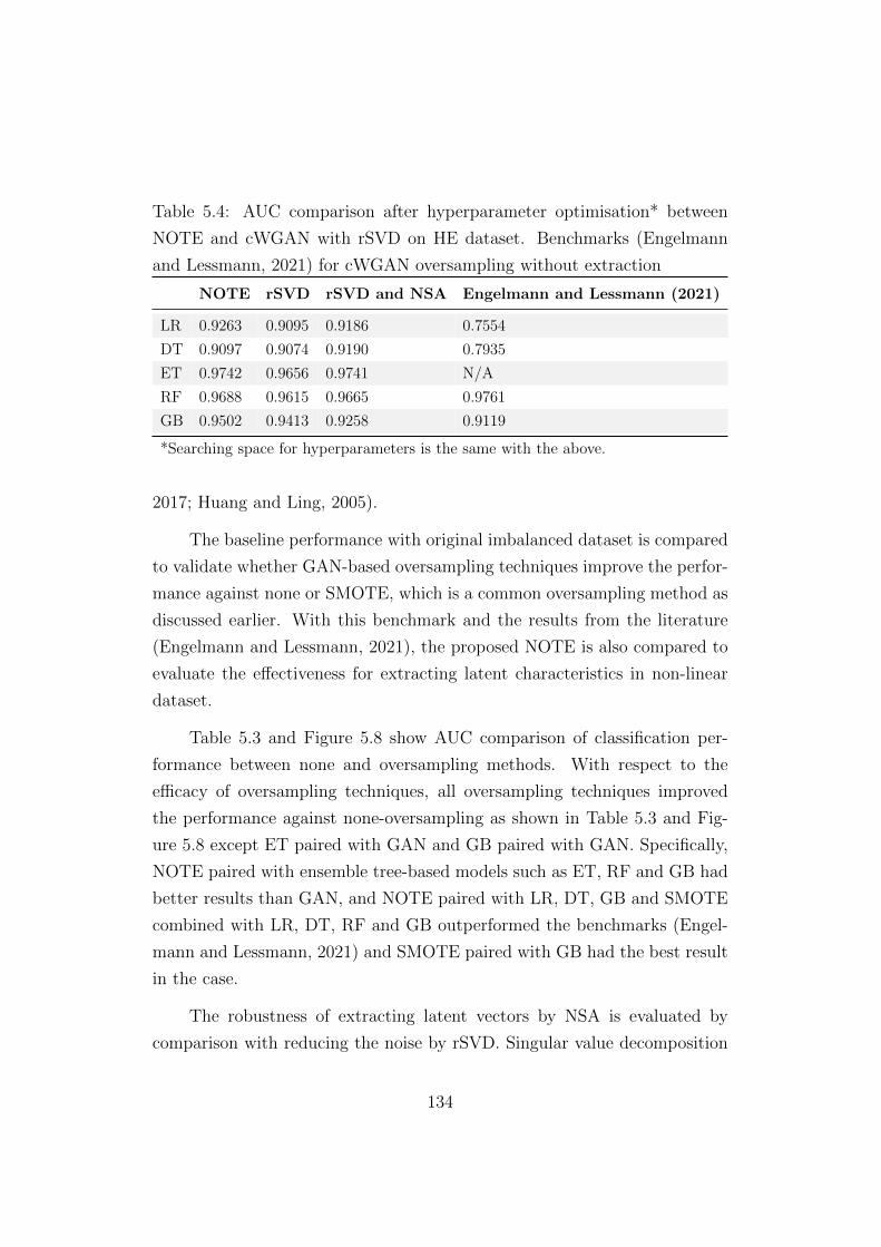
Table 5.4: AUC comparison after hyperparameter optimisation* between
NOTE and cWGAN with rSVD on HE dataset. Benchmarks (Engelmann
and Lessmann, 2021) for cWGAN oversampling without extraction
NOTE rSVD rSVD and NSA Engelmann and Lessmann (2021)
LR 0.9263 0.9095 0.9186 0.7554
DT 0.9097 0.9074 0.9190 0.7935
ET 0.9742 0.9656 0.9741 N/A
RF 0.9688 0.9615 0.9665 0.9761
GB 0.9502 0.9413 0.9258 0.9119
*Searching space for hyperparameters is the same with the above.
2017; Huang and Ling, 2005).
The baseline performance with original imbalanced dataset is compared
to validate whether GAN-based oversampling techniques improve the perfor-
mance against none or SMOTE, which is a common oversampling method as
discussed earlier. With this benchmark and the results from the literature
(Engelmann and Lessmann, 2021), the proposed NOTE is also compared to
evaluate the effectiveness for extracting latent characteristics in non-linear
dataset.
Table 5.3 and Figure 5.8 show AUC comparison of classification per-
formance between none and oversampling methods. With respect to the
efficacy of oversampling techniques, all oversampling techniques improved
the performance against none-oversampling as shown in Table 5.3 and Fig-
ure 5.8 except ET paired with GAN and GB paired with GAN. Specifically,
NOTE paired with ensemble tree-based models such as ET, RF and GB had
better results than GAN, and NOTE paired with LR, DT, GB and SMOTE
combined with LR, DT, RF and GB outperformed the benchmarks (Engel-
mann and Lessmann, 2021) and SMOTE paired with GB had the best result
in the case.
The robustness of extracting latent vectors by NSA is evaluated by
comparison with reducing the noise by rSVD. Singular value decomposition
134

Figure 5.10: Comparison of SHAP feature importance on RF of NOTE,
where en1, en2 and en3 are latent representation extracting from NSA
(SVD) for matrix decomposition has been commonly used for reducing di-
mensionality, analysing and compressing data (Erichson et al., 2019b).
Although SVD is computationally expensive, rSVD with the concept of
randomness has been introduced to reduce the computational cost and allow
the scalable transformation of matrix and capture the latent information in
the dataset (Erichson et al., 2019a). Since Engelmann and Lessmann (2021)
indicated the non-linearity for HE dataset in the paper, the rSVD method
can also be applied for the reconstruction of data. The proposed NOTE
is compared with cWGAN-based oversampling techniques through rSVD to
check which methods are more effective to enhance the performance of cW-
GAN for generating plausible synthetic distribution, and the performance of
classifiers for predicting classification.
Table 5.4 and Figure 5.9 show AUC comparison with five classifiers and
three cases for capturing the latent features by NOTE, cWGAN combined
135

Figure 5.11: SHAP value plot for individual sample predicted by RF of
NOTE
Figure 5.12: SHAP decision plot for individual sample predicted by RF of
NOTE
with rSVD and cWGAN combined with both rSVD and NSA against cW-
GAN only on the dataset. When compared to the benchmarks by Engelmann
and Lessmann (2021), AUCs were improved for all models except RF. These
results also proved that the latent information could be acquired and be re-
flected or some noise could be reduced through the reconstruction methods
if NSA or rSVD is conducted prior to the process of cWGAN oversampling.
It can be analysed that both NOTE and cWGAN paired with LR, DT
and GB through rSVD have better AUCs than cWGAN only without the
process of denoising or reconstruction as shown in Table 5.4 and Figure 5.9.
136

Figure 5.13: SHAP value plot for individual sample predicted by LR of NOTE
Table 5.5: Features on HE dataset used in NOTEFeature Description Type
BAD* Applicant paid loan, or applicant defaulted on loan or seriously delinquent N (Not defaulted = 0) / Y (Defaulted = 1)
LOAN Amount of the loan request integer
MORTDUE Amount due on existing mortgage integer
VALUE Value of current property integer
REASON DebtCon = debt consolidation; HomeImp = home improvement category
JOB Six occupational categories (Other, ProfExe, Office, Sales, Mgr, Self) category
YOJ Years at present job integer
DEROG Number of major derogatory reports integer
DELINQ Number of delinquent credit lines integer
CLAGE Age of oldest credit line in months real
NINQ Number of recent credit inquiries integer
CLNO Number of credit lines integer
DEBTINC Debt-to-income ratio real
*BAD is a feature for class label.
Especially, the AUC 0.9656 of cWGAN paired with ET through rSVD
on the dataset as shown in Table 5.4, has a difference (0.86) with the re-
sult of AUC 0.9742, which was obtained by NOTE. This implies that the
denoising process on non-linear dataset can also enhance the performance of
classification as similar to the process of extracting information.
Furthermore, the fact that AUCs were improved for all models except
RF as shown in Table 5.4 and Figure 5.9 shows that the proposed NOTE
successfully extracted latent vectors from the original non-linear dataset and
hence, AUCs were improved for LR, DT and GB as Engelmann and Less-
mann (2021) proved that HE dataset is strongly non-linear. Therefore, the
effectiveness of extracted latent features was demonstrated by using NSA
and by comparing NSA with denoising method by rSVD on non-linear credit
scoring dataset.
As a result, it was validated as an effective approach for improving clas-
sification performance to use the proposed NOTE paired with tree-based
137

ensemble classifiers if extracting latent vectors by NSA or reducing noise by
rSVD is applied to non-linear and imbalanced dataset as Engelmann and
Lessmann (2021) advised tree-based models in the paper, and their bench-
mark performance by Engelmann and Lessmann (2021) was improved further
by NSA or rSVD to extract latent vectors. This means that NOTE success-
fully proposed a novel architecture of a non-parametric model for non-linear
and imbalanced dataset.
Figure 5.14: Comparison of feature importance on tree-based models of
NOTE, where en1, en2 and en3 are latent representation extracting from
NSA
138

Figures 5.10, 5.11, 5.12 and 5.13 explain the prediction by NOTE. Figure
5.10 shows the global interpretability of the prediction as the average of
SHAP values for feature importance on all samples. Figure 5.11 shows local
interpretability of a certain sample for RF of NOTE as an example. In
addition, Figure 5.12 shows the decision path of the same sample starting
from the bottom for the prediction similar to DT, and Figure 5.13 shows local
interpretability of the same sample for LR of NOTE. The interpretability
is analysed by SHAP which measures the contribution of features to the
prediction for credit scoring. As shown in Figure 5.10, ‘DEBTINC’, ‘LOAN’
and ‘en3’ are the three most important features for the prediction on HE
dataset in general. Especially, the fact ‘en3’ is one of the top three features
indicates that NSA captured non-linearity successfully on HE dataset.
As discussed earlier, these figures can be described with ‘TreeExplainer’
on all tree-based models and ‘LinearExplainer’ on LR. These explainers al-
low to understand the models and analyse the reasons for explainability as
XAI since the explainability is regarded as the key factor for both financial
institutions and credit applicants. Therefore, the proposed NOTE enabled
the interpretability for credit scoring.
On the other hand, Figure 5.14 shows the comparison of traditional
feature importance between the proposed tree-based models such as DT,
ET, RF and GB on NOTE across the entire samples.
Finally, NOTE achieved the explainability aspect for practical applica-
tion in credit scoring as XAI combined with SHAP as well as high predictive
performance.
5.5 Conclusion
In this paper, a novel oversampling technique named NOTE was proposed
for the problem of imbalanced class in non-linear credit scoring dataset. The
evaluation was performed with three oversampling techniques, two extraction
139

methods and five different classification algorithms against the benchmarks.
The results showed that NOTE generated the minority class success-
fully with the combination of advantages of NSA, cGAN and WGAN. The
classification performance, hence, was significantly improved by the proposed
NOTE against the standard model as LR on non-linear imbalanced credit
scoring dataset and previous research about cWGAN-based oversampling for
class imbalance. Furthermore, since NOTE is explainable by ‘TreeExplainer’
and ‘LinearExplainer’ both locally and globally for the prediction as well
as stable for non-linear dataset, this affords the key advantages to practical
application in credit scoring.
Future work could use deep learning models such as Convolutional Neu-
ral Networks (CNN) combined with tree-based ensemble models of NOTE
as a hybrid for higher robustness in extracting non-linearity. Although CNN
has been frequently used in voice recognition, natural language processing
and computer vision problems, CNN could be applied to solve supervised
classification problems on tabular datasets. The combination of the superior
ability of CNN as feature extractor and the embedded method of tree-based
NOTE as feature selector, can finally improve the classification performance
by capturing non-linear characteristics and patterns in the datasets.
In addition, more heavily or absolutely imbalanced non-linear datasets
in the diverse types of domain could be employed to validate the performance
of NOTE for further study.
140

Chapter 6
GAN-based Imputation
Techniques for Missing Values
6.1 Introduction
Credit scoring can be modelled from records or datasets that contain demo-
graphic, asset, income, payment behaviour, etc., as input features in relation
to the creditworthiness. However, datasets in the real-world often have miss-
ing values or incomplete features for many reasons such that observations
were not recorded and features were corrupted (Horton and Kleinman, 2007;
Ibrahim et al., 2005; Yoon et al., 2018). For example, UCI Machine Learning
Repository (Dua et al., 2017), which is a frequently used dataset collection,
shows that 45% of datasets in the repository contain missing values (Garcıa-
Laencina et al., 2010) and incomplete data are common for every case in
observational studies such as social science and clinical trials (Li et al., 2015;
Roderick et al., 2002; Schafer, 1997).
The issue of missing values reduces the number of available samples for
analysis or might distort analysis when classification models make prediction
process (Cheema, 2014; Jerez et al., 2010; McKnight et al., 2007). Hence,
this drawback affects the performance of models as mentioned above, where
141

missing values or incomplete dataset can lead to the misclassification for
the application of creditworthiness. In addition, ML models generally need
complete data to be trained before the process of prediction (Ruiz-Chavez
et al., 2018; Smieja et al., 2018). Due to this necessity of completeness in
datasets for statistical and ML models, it is vital to deal with missing values
appropriately (Bertsimas et al., 2017).
Nevertheless, the problem has often been ignored, or basic and simple
methods such as removing samples with missing values or mean imputation
in missing values, have been applied to cope with incomplete datasets in the
analysis of credit scoring (Jerez et al., 2010; Nationalbank, 2004). The aim
of dealing with missing values is to estimate the values similar to underlying
complete dataset as close as possible (Bertsimas et al., 2017). The methods
can be categorised into two groups (Kline, 2015), which are deletion and
imputation.
Since deletion methods reduce the size of samples which have missing
values, it might lead to the distortion for analysis as discussed and it cannot
be the best way. Therefore, if the large portion of the samples comprises
incomplete data, it leads to errors by the reduced size of samples (Little and
Rubin, 2019). On the other hand, imputation methods, which are to replace
incomplete portion of data with substituted values, are frequently employed.
This way is called as missing data imputation (Salgado et al., 2016). This im-
putation is considered as the most appropriate and valid approach for dealing
with incomplete datasets (Florez-Lopez, 2010). Imputation methods can be
grouped into statistical and machine learning (ML) methods by approaches
or generative methods by characteristics of imputation.
Therefore, the ability of handling missing values or incomplete datasets
is important and required for classification to avoid large error or false esti-
mation. Many studies based on statistics and ML have been introduced in
order to handle this problem. They have shown that any methods do not
guarantee the efficiency of the proposed methods. This means that the effi-
cacy depends on the domain of the problem (e.g., number of samples, number
142

of features, pattern of missing data and the percentage of missing data in
the dataset) (Jerez et al., 2010).
This study, hence, extending the GAIN-based imputation technique,
proposes a novel imputation method named DITE (Denoising Imputation
TEchniques for missingness in credit scoring) in order to solve the issues of
missing values in credit scoring dataset for classification. First, the miss-
ingness is generated in the complete dataset. Then, the missing values in
dataset are imputed by statistical and ML methods to see how the imputa-
tion performance is affected by various imputation techniques. Especially,
imputation methods using ML techniques such as Multiple Imputation by
Chained Equations (MICE) (Buuren and Groothuis-Oudshoorn, 2010), Miss-
Forest (Stekhoven and Buhlmann, 2012), Generative Adversarial Imputation
Nets (GAIN) (Yoon et al., 2018), and the variants of GAIN in the domain
of credit scoring will be analysed comparatively.
The aim of this study is to examine the robustness and effectiveness of
DITE as well as to compare the imputation performance with the variants
of GAIN, GAIN, MissForest and MICE.
The key contributions of this study are as follows:
• To demonstrate the effectiveness of denoising method by randomised
singular value decomposition (rSVD) in a credit scoring dataset
• To present the advancement of GAIN imputation paired with rSVD by
improving the imputation performance in an incomplete credit scoring
dataset, compared with the benchmarks by original GAIN, the variants
of GAIN, and conventional statistical and ML imputation approaches
• To propose an architecture of credit scoring model for datasets with
missingness
• To suggest new benchmark results that outperform the state-of-the-art
model by Yoon et al. (2018) on DC (Default of Credit card clients)
dataset for missing value imputation
143

• To enable the practical application of imputation for missingness on
incomplete credit scoring datasets
We hypothesise that the proposed DITE will not only reduce the noise
in redundant and noisy datasets, but also build a model that are capable for
suitable imputation on incomplete credit scoring datasets.
The remainder of this paper is organised as follows: Section II discusses
the related studies and identifies the gaps in the current technologies. Section
III describes the proposed DITE with its novel concepts. Section IV presents
the results evaluating the performance of DITE with the benchmarks on
the recent studies. Finally, Section V concludes with the summaries of the
findings from this study.
6.2 Related Work
This section discusses the related studies on imputation methods and mech-
anism for missing values.
6.2.1 Imputation Methods for Missing Values
Imputation methods for missing values can be grouped into two ways, which
are generally simple imputation methods and multiple imputation methods.
For single imputation methods such as mean/median/mode and regres-
sion, missing values are substituted with a single estimated value (Donders
et al., 2006). Among them, mean imputation (Little and Rubin, 1989) to sub-
stitute missing value with overall sample mean is easily and generally used
(Hammad Alharbi and Kimura, 2020). However, this method can under-
estimate the standard error and variance, and distort the basic distribution
of data by ignoring the relations between features (Vriens and Melton, 2002).
Regression imputation using existing (or complete) data in features by re-
gression model to substitute missing value with predicted value, would be
144

Table 6.1: The examples of imputation methods
Method Category Reference
Mean imputation Mean Little and Rubin (1989)
Expectation Maximisation (EM) EM Dempster et al. (1977)
EM with bootstrapping EM Honaker et al. (2011)
K-Nearest Neighbour (KNN) KNN Troyanskaya et al. (2001)
MICE ML-based regression trees Buuren and Groothuis-Oudshoorn (2010)
MissForest ML-based random forest Stekhoven and Buhlmann (2012)
GAIN GAN-based neural networks Yoon et al. (2018)
an advanced method when compared to mean imputation. However, this
method can also have the same issue regarding the standard error and vari-
ance (Baraldi and Enders, 2010). Therefore, the deficiency of single impu-
tation methods does not reach the acceptable level of performance (Awan
et al., 2021).
For multiple imputation methods such as Expectation Maximisation
(EM) (Dempster et al., 1977) and MICE (Buuren and Groothuis-Oudshoorn,
2010), missing values are replaced with a set of values and these methods
have been proposed to overcome the limitation of simple imputation meth-
ods (Yuan, 2010). When compared to single imputation, multiple imputation
produces several values by predictive distribution and a set of values is com-
bined to a single value after the process of analysis to impute missing values.
However, this method costs more computationally since optimal iterations
for convergence are not easy to be figured out (Kline, 2015), although multi-
ple imputation allows to avoid unreliability of single imputation (Dong et al.,
2021). In addition, MICE which is a regression-based method such as LR,
has the limited performance to capture non-linearity (Seaman et al., 2012).
This weakness, hence, might not reflect the interaction between features when
taking imputation.
On the other hand, ML methods such as K-Nearest Neighbour (KNN)
(Troyanskaya et al., 2001) imputation and MissForest (Stekhoven and Buhlmann,
2012) have been proposed and used commonly to impute missing values since
these methods do not need the assumption for the distribution of data (Jerez
145

et al., 2010). Since MissForest is based on RF, it has shown the strengths
to handle the non-linearity for replacing missing values with estimation in
dataset (Stekhoven and Buhlmann, 2012). The studies have shown that the
imputation by MissForest generally performs better than that of MICE (Shah
et al., 2014).
Furthermore, Generative Adversarial Imputation Networks (GAIN) (Yoon
et al., 2018) as a GAN-based substitution approach has been proposed and
shown promising results to fill the missing values in tabular datasets. Yoon
et al. (2018) introduced the generative model to estimate the missing values
using GAN architecture in an adversarial way. As discussed, GAN as a gen-
erative model has been proved that it is accurate and effective for capturing
the latent patterns in complex and non-linear datasets since the generative
models are capable of modelling the distribution of original data (Awan et al.,
2021). The GAIN using GAN has also been proved by Yoon et al. (2018) in
the study that it is more robust than existing imputation methods such as
AutoEncoder and MissForest. Table 6.1 shows the examples of imputation
methods.
Nazabal et al. (2020) proposed the HI-VAE model to estimate hetero-
geneous incomplete (HI) tabular data with mixed continuous and discrete
values, based on variational autoencoder (VAE). They also showed that pre-
dictive performance on complete data through HI-VAE has better results
than original incomplete data. Camino et al. (2019) suggested a methodol-
ogy to improve imputation performance of GAIN and VAE, and showed that
their methods have better imputation performance on real-world datasets.
With the variants of GAIN algorithms using advancement of GAN, Halmich
(2020) developed Wasserstein GAIN (WGAIN) imputation techniques to im-
prove the stability of the GAIN imputation method. The study showed com-
parative results against the benchmarks (Yoon et al., 2018) using WGAIN
and achieved acceptable performance. Awan et al. (2021) also proposed a
variant of GAIN algorithm as CGAIN using Conditional GAN (CGAN) to
generate synthetic values for missingness. The study showed comparative
results of performance for CGAIN against the benchmarks of existing impu-
146

Figure 6.1: The complete data without missing values on the features (a) and
incomplete data with missing values on the features (b), where x1, x2, · · · , xd
represent the features and t denotes the label (Garcıa-Laencina et al., 2010)
tation methods.
6.2.2 Mechanism for Missing Values
Since it depends significantly on the mechanism of missingness to deal with
the problem of missing values, the nature and effect of missingness needs to
be analysed and taken into account on credit scoring datasets (Florez-Lopez,
2010).
Dataset without missing values can be denoted as X and dataset with
missing values can be denoted as XM . Therefore, XM consists of two parts
as follows:
XM = Xo, Xm (6.1)
where Xo is an observed and complete set, and Xm is a missing and in-
complete set. M can be used as indicator matrix known generally for missing
data. M indicates which inputs of XM are observed or complete and which
features of XM are incomplete or missing, and is a binary matrix (Garcıa-
Laencina et al., 2010). Figure 6.1 shows the missingness in the dataset.
Since missing values Xm can be estimated, based on observed values
Xo by imputation methods, there are three different types of missing data
147

according to the characteristic of missingness, which means how the com-
ponents of features became missing (Rubin, 1976). The characteristics of
missingness can be categorised as follows (Garcıa-Laencina et al., 2010):
1. Missing completely at random (MCAR)
2. Missing at random (MAR)
3. Missing not at random (MNAR)
MCAR occurs when the probability P is independent of both observed
and missing data and shows high level randomness, where the probability P
is that the data or features are missing (Garcıa-Laencina et al., 2010).
P (M |Xm) = P (M) (6.2)
MAR occurs when the missingness has dependency only on the observed
data regardless of missing data and shows mid level randomness (Garcıa-
Laencina et al., 2010).
P (M |Xm) = P (M |Xo) (6.3)
MNAR occurs when the probability P is dependent on both observed
and missing data and shows low level randomness, where the probability P
is that the data or features are missing (Garcıa-Laencina et al., 2010).
P (M |Xm) = P (M |Xo, Xm) (6.4)
The classification for characteristics of missingness is important since
imputation methods can be applied in a certain pre-condition or assumption.
When the data is in the category of MCAR or MAR, missing data is an
ignorable mechanism (Garcıa-Laencina et al., 2010). This means that when
MCAR or MAR occurs, imputation methods for missing data can be applied
in the analysis of data regardless of the reason for missingness and it is
possible to expect missing values (Schafer, 1997). Due to this reason, most
148

research for missing data imputation have been studied when missingness
occurs in MCAR or MAR (Enders and Gottschall, 2011; Garcıa-Laencina
et al., 2010). In this paper, the experiment will be performed to approximate
and impute values for missing data under the assumption of MCAR.
6.3 DITE: Denoising Imputation TEchniques
for missingness in credit scoring
The DITE consists of four stages, which are as follows:
1. Collecting DC dataset
2. Rescaling and denoising original dataset by rSVD
3. Imputing the values generated by GAIN for missing data in incomplete
dataset
4. Predicting the classification on complete dataset
These stages need to process sequentially in order to obtain the neces-
sary levels of effectiveness.
Default of Credit card clients (DC) dataset (Yeh and Lien, 2009) con-
tains demographic information, history of payment, default payment and
delinquency for the samples of credit card clients. It comes from previ-
ous paper of credit scoring literature and UCI Machine Learning Repos-
itory (UCI MLR) (Dua et al., 2017). It consists of 30,000 samples with
23,364 good credit samples and 6,636 bad credit samples, respectively. Bad
credit samples are defined as the cases where the target feature named ‘de-
fault.payment.next.month’ is specified as 1, which means the client has de-
faulted on the payment. On the other hand, good credit samples are classified
as the cases that the label is specified as 0, which means the client has not
defaulted on the payment. This is a binary class label. The dataset does not
149

contain missing values originally and was used due to the benchmark in the
results (Awan et al., 2020; Camino et al., 2019; Halmich, 2020; Yoon et al.,
2018).
The initial dataset shows the percentage of minority class in total as
22.12 % and Imbalance Ratio (IR) as 3.52, which is the number of the ma-
jority class divided by the number of the minority class. The dataset contains
23 features that can directly be interpreted into a credit scoring system, ex-
cluding target feature.
The concepts and methodologies for replacing missing values in the
dataset with the estimation are introduced and described in this section.
In order for filling missing values in incomplete features of the dataset,
the dataset can be substituted with the values obtained by statistical meth-
ods such as mean imputation (simple imputation), ML methods such as
MICE, KNN, MissForest, and neural network (NN) methods such as GAIN.
The results will be analysed comparatively as to whether the proposed model
DITE is as robust against the benchmarks as GAIN-based methods, Miss-
Forest, MICE and simple imputation.
Before rSVD is applied for removing the noise in dataset, normalising
the dataset can be conducted to make the training of GAIN less sensitive
to the scale of features. It rescales the range of values in the dataset to be
inside the interval [0, 1], and enhances the performance of synthesising the
data by GAIN. Since GAIN is one of the algorithms as NN, NN is sensitive
to the scale when it weights input values.
The normalisation is expressed as follows:
Normalised(Vi) =Vi −min(Vi)
max(Vi) −min(Vi)(6.5)
where Vi is a value of feature, and max(Vi) and min(Vi) are the maxi-
mum and minimum of values in features, respectively.
After normalising the values in the dataset, rSVD is applied to the
normalised dataset to remove the noise in order to enhance the performance
150

Figure 6.2: The conceptual architecture of rSVD
of GAIN as well. It is common that real-world credit scoring datasets have
noise and redundant features (Xia et al., 2017). rSVD can thus be an effective
method to reduce the noise before the process of imputation by GAIN.
Singular value decomposition (SVD) for matrix decomposition has been
commonly used for reducing dimensionality and noise, analysing and com-
pressing data, especially in image processing. The compressed image with
reduced noise and extracted characteristics can be obtained by SVD.
SVD can also be applied to the imputation for missing values in tabular
dataset, based on the assumption that the dataset consists of noisy samples of
a linear combination with principal factors (Bertsimas et al., 2017). Through
SVD, the principal factors, which are called as eigenvectors, can be obtained.
These eigenvectors enhance GAIN algorithm to capture the patterns and
characteristics of the dataset and estimate the values in the missing part of
the dataset.
Given a matrix M ∈ Rm×n with m×n, SVD can be expressed as follows:
M = UΣV T (6.6)
where matrix U = [u1, · · · , um] ∈ Rm×m, matrix V = [v1, · · · , vm] ∈
151

Rn×n, and U and V are orthogonal. The left singular vectors in U show a
basis for column space (the range) and the right singular vectors in V show
a basis for domain space (the row) of the matrix M (Erichson et al., 2019c).
The rectangular matrix Σ ∈ Rm×n has the corresponding singular values σ1
≥ · · · ≥ σn ≥ 0 in diagonal, representing the spectrum of data (Erichson
et al., 2019c). That is,
M = UΣV T = [u1, · · · , um]diag(σ1, · · · , σn)[v1, · · · , vm]T (6.7)
Figure 6.2 shows the conceptual architecture of rSVD. Although SVD
is computationally expensive, rSVD with concept of randomness has been
introduced to reduce the computational cost. This concept allows the scalable
transformation of matrix and captures the latent information in the dataset
(Erichson et al., 2019a). In addition to the application of rSVD, Camino et al.
(2019) and Hammad Alharbi and Kimura (2020) proved that imputation
performance of GAIN was improved by normalised dataset. Therefore, a
promising performance would be expected if denoising method by rSVD could
be combined with the normalised dataset before imputation techniques by
GAIN.
Following rescaling and denoising methods by normalisation and rSVD,
DITE performs GAIN-based imputation to replace the missing values with
generated data on the incomplete dataset.
GAIN (Yoon et al., 2018) was proposed to deal with the problem of
missing values in dataset using the architecture of GANs (Goodfellow et al.,
2014). Missing values are imputed by the conditional distribution or joint
distribution of complete data matrix X as mentioned earlier in Section 6.2.
Since GANs generate synthetic data through adversarial learning of gener-
ator and discriminator, missing values can be imputed using distribution of
synthetic data rather than using expectation of multiple imputations such as
MICE (Royston et al., 2011). Specifically, the discriminative models such as
MICE and MissForest learn a function that maps the input x into output y
and are able to fill the missing values using conditional probability P (y|x).
152

Figure 6.3: The architecture of GAIN
On the other hand, the generative models such as EM, Denoising AutoEn-
coder (DAE) and GAIN learn a probability distribution of data and are able
to fill the missing values using joint probability P (x, y).
GAIN algorithm is based on the architecture of GAN and consists of
generator G and discriminator D as same with GAN. However, GAIN algo-
rithm has unique characteristics when compared to standard GANs, and the
objective of GAIN is different from the objective of GAN. Although GAN is
trained to generate synthetic distribution from original distribution and to
153

distinguish whether the entire generated data is real or fake, GAIN is trained
to fill in incomplete data of samples and to distinguish whether the gener-
ated values are real or fake, i.e. generator G generates plausible components
for missing values in samples using the distribution of original data and dis-
criminator D discriminates between each plausible generated (or imputed)
components and observed components in the data (Yoon et al., 2018).
G in GAIN takes the inputs: data matrix, random matrix and mask
matrix. The mask matrix represents whether a value is present or absent,
i.e., the marking of missing value, where a presence of value in matrix is
marked as 1, while an absence of value in matrix is marked as 0. D in GAIN
predicts the complete estimated mask matrix whose components show, for
each component of data, whether the corresponding input value is observed
or not (missing) in the original data by hint matrix from hint generator
(Awan et al., 2021). Figure 6.3 shows the architecture of GAIN.
To compare GAN with GAIN architecture, two-player minmax game of
GAN can be expressed with objective function as follows:
minGmaxDV (D,G) = Ex∼Pdata(x)[logD(x)] + Ez∼Pz(z)
[log(1 −D(G(z)))]
(6.8)
Based on the architecture of GAN, the objective function of GAIN can
be expressed as follows:
minGmaxDV (D,G) = EX,M,H [MT logD(X,H)+(1−M)T log(1−D(X,H))]
(6.9)
where M is a mask matrix, which indicates the position of missing values
in original incomplete matrix X, and H is a hint matrix, which prevents
the discriminator D from learning dominantly when compared to generator
G, and D(X,H) = M is the probability such that the imputed values are
observed values.
154

Generator G takes inputs as data matrix X, random matrix Z and mask
matrix M , and generates output as imputed matrix X. Discriminator D
takes inputs as imputed matrix X and hint matrix H, and generates output
as an estimated mask matrix M = D(X,H)
The objective of generator G in GAIN is to generate plausible synthetic
values as close as the observed value that mask matrix M indicates it equals
to 1 (observed), in order to deceive the discriminator D that discriminates
the plausible synthetic value as the real or observed value.
On the other hand, the objective of discriminator D in GAIN is to
distinguish the observed value as the observed value that mask matrix M
indicates it equals to 1 (observed), and distinguish the missing value as the
missing value that mask matrix M indicates it equals to 0 (missing).
The process of GAIN is also a two-player minmax game as discussed
earlier.
The loss of generator G in GAIN consists of two parts since G outputs
the imputed matrix for both the observed values and the missing values. The
first part shows the loss of imputed values and the second part represents
the loss of observed values (Awan et al., 2021). The loss of generator G in
GAIN, hence, can be expressed as follows:
LG(m, m, b) = −∑i:bi
(1 −mi)log(mi) + αd∑
j=1
miLM(xi, xi) (6.10)
where α denotes a positive hyperparameter and LM(xi, xi) is as follows
(Yoon et al., 2018):
LM(xi, xi) =
mi(xi − xi)2, if xi is continuous
mi(−xilog(xi)), if xi is binary(6.11)
The loss of discriminator D in GAIN can also be written by the form of
cross entropy as follows:
155

Figure 6.4: The system architecture of DITE
LD(m, m, b) =∑i:bi
(milog(mi) + (1 −mi)log(1 − mi)) (6.12)
where bi is the ith element of a random variable B = (B1, ..., Bd) ∈0, 1d, which is acquired by sampling k from 1, ..., d uniformly at random
and mi is the ith element of mask matrix M (Yoon et al., 2018). Afterwards
setting
Bj =
1, if j = k
0, if j = k(6.13)
The imputation performance of DITE is compared against the bench-
marks, which are MissForest as ML-based random forest imputation method
and MICE as ML-based regression trees imputation method as well as the
variants of GAIN approaches.
Following imputing the values generated by DITE, DITE performs the
156

Table 6.2: RMSE comparison for imputation performance of the proposed
DITE against the benchmarks on default credit card with 5%, 10%, 15% and
20% missing data
5% 10% 15% 20%
DITE 0.0724±0.0009 0.0763±0.0007 0.0818±0.0033 0.0857±0.0005
GAIN∗ 0.1447±0.0016 0.1482±0.0005 0.1532±0.0005 0.1561±0.0012
GAIN (Awan et al., 2021) 0.2428±0.0093 0.2109±0.0344 0.2442±0.0089 0.2426±0.0090
CGAIN (Awan et al., 2021) 0.2329 ±0.0039 0.2009±0.0022 0.2314 ±0.0035 0.2213±0.0099
MissForest (Awan et al., 2021) 0.2902±0.0010 0.2439±0.0079 0.2672±0.0025 0.2646±0.0026
MICE (Awan et al., 2021) 0.2479 ±0.0079 0.2491±0.0085 0.2479 ±0.0074 0.2480±0.0091
*Implemented
Figure 6.5: RMSE comparison for imputation performance on missingness
prediction with complete dataset. Overall, Figure 6.4 shows the system ar-
chitecture of DITE.
6.4 Results
To validate the efficacy of DITE (denoising GAIN-based imputation method)
for missing values or incomplete data, missing values are generated randomly
with the percentage of 5%, 10%, 15%, 20%, 50% and 80%. Removing values
in the dataset is based on the assumption of MCAR in the complete dataset.
157

Table 6.3: RSME comparison for imputation performance of the proposed
DITE against GAIN-based imputation methods on default credit card with
20% missing data
20%
DITE 0.0857±0.0005
GAIN* 0.1561±0.0012
GAIN+vs** (Camino et al., 2019) 0.1190±0.0040
GAIN (Yoon et al., 2018) 0.1858±0.0010
CGAIN (Awan et al., 2021) 0.2213±0.0099
WGAIN (Halmich, 2020) 0.2712±0.0014
*Implemented **Variables split
The performance of DITE is evaluated by the metric as Root Mean
Square Error (RMSE) in order to validate the imputation performance. The
RMSE is the root of mean squared error (MSE) for the prediction f(x) with
respect to label y. MSE can be expressed as follows:
MSE(f(x)) = E[(f(x)− y)2] =1
m
m∑i=1
(f(xi)− yi)2 =
∫x∼D
(f(x)− y)2p(x)dx
(6.14)
where D is the distribution of data and p(·) is the probability density
function.
Before the classification performance through imputation is compared
between DITE, GAIN, MissForest, and MICE as benchmarks, the imputation
performance of DITE on DC dataset needs to be evaluated. The proposed
DITE is compared against the state-of-the-art benchmarks of existing pop-
ular imputation methods such as the variants of GAIN: GAIN+vs (Camino
et al., 2019), GAIN (Yoon et al., 2018), CGAIN (Awan et al., 2020), WGAIN
(Halmich, 2020) and the standard ML-based imputation method such as
MissForest and MICE.
158

Figure 6.6: RMSE comparison for GAIN-based imputation methods on de-
fault credit card with 20% missing data
Table 6.2 and Figure 6.5 show RMSE comparison for imputation perfor-
mance where the percentage of missing values ranges from 5% to 20%. The
proposed DITE showed the best imputation performance when compared
to other approaches. As can be seen, DITE outperformed the benchmarks
on four different proportions of missing values. Furthermore, GAIN-based
imputation methods showed superior results to ML-based method.
Table 6.3 and Figure 6.6 show RSME comparison for imputation per-
formance between GAIN-based imputation methods on 20% missing data.
DITE outperformed all other GAIN-based imputation models.
With the justification by the results of Table 6.3 and Figure 6.6, the
four best models need to be analysed further on varying proportion of miss-
ing values since RMSE 0.2 can be regarded as the threshold for imputation
performance on models and different percentage of missing values, as shown
in Figure 6.6.
Table 6.4 and Figure 6.7 show RMSE comparison for imputation perfor-
mance between the four best models, where the percentage of missing values
ranges from 20% to 80%. The proposed DITE showed the best imputation
159

Table 6.4: RMSE comparison for imputation performance of the proposed
DITE against the best four benchmarks of GAIN-based imputation on default
credit card with 20%, 50% and 80% missing data
20% 50% 80%
DITE 0.0857±0.0005 0.1292±0.0068 0.1449±0.0199
GAIN* 0.1561±0.0012 0.1926±0.0179 0.2787±0.0052
GAIN+vs**(Camino et al., 2019) 0.1190±0.0040 0.1840±0.0040 0.2550±0.0030
GAIN (Camino et al., 2019) 0.1230±0.0010 0.1940±0.0020 0.2700±0.0050
*Implemented **Variables split
performance when compared to other approaches. In addition, DITE out-
performed the benchmarks on severe condition having 80% missing values.
As a result and as expected, the imputation performance of all GAIN-
based models decreases when the percentage of missingness increases. How-
ever, GAIN-based imputation approaches outperformed ML-based imputa-
tion methods such as MICE and MissForest, as shown in Figure 6.5.
This implies that GAIN-based models have robust imputation power
since they are updated by the feedback using the loss of cross entropy from
the discriminator as well as the observed values in the dataset. GAIN-based
models, hence, have the capability to resist high proportion of missingness in
the dataset. With this reason, DITE showed the stable results comparatively
although the proportion of missing data increases as shown in Figure 6.7.
Therefore, the advancement of GAIN imputation paired with rSVD was
presented by improving the imputation performance on incomplete credit
scoring dataset, compared with the benchmarks by original GAIN, the vari-
ants of GAIN, and conventional statistical and ML imputation approaches.
Finally, DITE successfully proposed a novel architecture of credit scoring
model for datasets with missingness.
160

Figure 6.7: RMSE comparison for imputation performance of the proposed
NITE against the best four imputation methods on default credit card with
20%, 50% and 80% missing data
6.5 Conclusion
In this paper, a novel imputation technique named DITE was proposed for
the issue of missing values on credit scoring dataset. Designing the method-
ology for generative model was focused by expanding the state-of-the-art
GAIN algorithm.
The empirical results showed that the proposed DITE generated the
synthetic values successfully for missingness in the dataset by the combina-
tion of the advantages of normalisation, rSVD and GAIN, with reflecting
the latent characteristics of the dataset. DITE outperformed the ML-based
methods such as MICE and MissForest, and the variants of GAIN such as
CGAIN and WGAIN, including GAIN in the imputation of missing values
on credit scoring dataset. This robust imputation approach as DITE could
finally result in the improvement of predictive performance for credit scor-
ing against the benchmarks of other completion methods. Therefore, DITE
can be applied to more accurate credit scoring, requiring the estimation of
missing values on complex tabular datasets.
161

Future work could extend this novel methodology to more complicated
areas such as text, voice recognition and missing image imputation.
162

Chapter 7
Conclusions
7.1 Introduction
In this thesis, the main purpose was focused on dealing with three key is-
sues of the modelling process for explainable and accurate credit scoring.
Three challenges were examined during developing credit scoring. First, the
interpretability in credit scoring as XAI was examined with respect to the
non-parametric approaches combining with the state-of-the-art SHAP val-
ues. In this experiment, the suitability of tree-based ensemble models was
also assessed on imbalanced credit scoring dataset. Second, class imbal-
ance on credit scoring was explored to quantify the prediction performance
through generative resampling methods, expanding the state-of-the-art GAN
algorithm paired with stacked autoencoder. Third, missingness on dataset
was examined to assess generative imputation approaches, expanding the
state-of-the-art GAIN algorithm. These three problems were handled by the
proposed novel models, named NATE, NOTE and DITE, respectively. This
thesis demonstrated the comparative results against the benchmarks to eval-
uate the proposed models. The proposed models achieved both explainability
and robustness aligned with the main aim of this research.
Specifically, NATE outperformed the industry standard LR model, which
163

was used as a benchmark model in this thesis, and successfully explained
the reasons for credit scoring by non-parametric tree-based approach with
SMOTE on real-world imbalanced GMSC dataset. NOTE outperformed
LR on non-linear, complex and imbalanced HE dataset, with extracting
non-linear patterns by NSA and reflecting the non-linear characteristics of
the minority class by cWGAN as well as with overcoming the limitation of
SMOTE and interpreting the non-parametric models. DITE outperformed
the state-of-the-art imputation methods by denoising dataset and generating
substituted values on DC dataset with missing values, as a result, and allows
to have potential for improving the predictive performance in credit scoring
model.
7.2 Summary of Contributions
At the end of this thesis, the contributions of this work are provided with the
summaries of each chapter in order to provide how this research contributes
to the domain of credit scoring to the readers.
• Chapter 2
1. explained theoretical concepts of machine learning, evaluation and
selection for machine learning models, and classification algorithms.
2. focused on ensemble models, i.e., non-parametric tree-based al-
gorithms to validate the suitability, stability and superiority for
the application of credit scoring in order to balance the trade-
off between model explainability and predictive performance with
reviewing the related literature of ensemble algorithms in the do-
main of credit scoring.
164

• Chapter 3
1. presented the overview about theoretical concepts and background
of credit scoring and the applicability of machine learning.
2. designed the general system architecture for credit scoring model
using machine learning as the process of development and imple-
mentation.
3. described the real-world credit scoring datasets and the prepro-
cessing methods of original raw datasets.
4. addressed the three primary issues in the process of system archi-
tecture, namely, model explainability, imbalanced class and miss-
ing values on credit scoring datasets, supported by the related
literature.
5. proposed the novel approaches using the state-of-the-art machine
learning techniques for dealing with the key issues of credit scor-
ing.
6. presented the results of the proposed models briefly as the show-
case of novel approaches.
• Chapter 4
1. addressed the issues of model explainability and imbalanced class
on credit scoring dataset with related work about SHAP and re-
sampling methods.
2. demonstrated the efficacy of non-parametric models on non-linear
GMSC (Give Me Some Credit) dataset for credit scoring
3. presented the standard oversampling method as SMOTE synthe-
sising the minority class in imbalanced dataset, compared with
undersampling method by NearMiss
4. proposed NATE as the system architecture of non-parametric ap-
proach on non-linear and imbalanced dataset for explainable credit
scoring.
165

5. suggested the results that SMOTE outperforms NearMiss on the
diverse imbalanced ratio of GMSC dataset and proved that over-
sampling performs better than undersampling to improve the clas-
sification performance.
6. achieved the explainability aspect for practical application in credit
scoring as XAI combined with SHAP as well as high predictive
performance of the proposed non-parametric model.
• Chapter 5
1. addressed the issues of model explainability and imbalanced class
on non-linear and complex dataset with related work about GAN-
based oversampling methods and generating tabular data by GAN.
2. demonstrated the effectiveness of extracted latent features using
NSA and compared NSA with denoising method by rSVD on non-
linear HE (Home Equity) dataset for credit scoring.
3. presented the advancement of cWGAN by overcoming the problem
of mode collapse in the training process of GAN and determined
the suitability, stability and superiority of cWGAN generating the
minority class on imbalanced dataset, compared with the bench-
marks by GAN and SMOTE.
4. proposed NOTE as a novel architecture of a non-parametric model
for non-linear and imbalanced dataset.
5. suggested new benchmark results that outperform the state-of-
the-art model by Engelmann and Lessmann (2021) on HE dataset
for classification performance.
6. enabled the explainability aspect of the proposed model for prac-
tical application in credit scoring as XAI.
• Chapter 6
1. addressed the issues of missingness in dataset with related work
about the conventional imputation approaches for missing values
and mechanisms of missingness.
166

2. demonstrated the effectiveness of denoising method by rSVD on
DC (Default of Credit card clients) dataset for credit scoring.
3. presented the advancement of GAIN imputation paired with rSVD
by improving the imputation performance on incomplete credit
scoring dataset, compared with the benchmarks by original GAIN,
the variants of GAIN, and conventional statistical and ML impu-
tation approaches.
4. proposed DITE as a novel architecture of credit scoring model for
datasets with missingness.
5. suggested new benchmark results that outperform the state-of-
the-art models by Yoon et al. (2018) on DC dataset for imputation
performance.
6. enabled the practical application of imputation for missingness on
incomplete credit scoring dataset.
7.3 Future Work
As further research and future work, the proposed models as NATE, NOTE
and DITE in this thesis can be extended to the followings.
NATE and NOTE as non-parametric tree-based models could be com-
bined with CNN as a hybrid for higher robustness in extracting non-linearity.
This hybrid approach could result in the improvement of predictive perfor-
mance of models with the strengths of NATE and NOTE in the aspects of
interpretability and explainability.
NOTE could be examined further in more sophisticated and compli-
cated form for generative performance, e.g., the distribution ratio of class
imbalance, absolute imbalanced class and multi-class distribution on the di-
verse domain of datasets. Furthermore, cost-sensitive loss function, as sug-
gested by Al-Sawwa and Ludwig (2020), could also be considered and merged
with NOTE as an algorithm-level approach. This method could lead to not
167

only the improvement of overall predictive performance of NOTE, but also
the improvement of the accuracy of the classification for the minority class.
This combination of data-level oversampling technique and algorithm-level
cost-sensitive classification approach could finally be an optimal solution for
imbalanced class.
DITE could be scrutinised further in more detailed experiments for im-
putation performance of the integer and categorical features, respectively
since DC dataset is composed of the features with both integer and cate-
gory. In other words, the imputation errors (RMSE) of DITE, the variants
of GAIN and GAIN could be compared for integer, continuous and categori-
cal features, respectively, as the missing rates increase on the diverse domain
of datasets. Furthermore, DITE could be examined in the environment of
absolutely skewed continuous features and highly imbalanced categorical fea-
tures at a certain missingness rate (e.g. 20%), as suggested by Dong et al.
(2021).
168

Appendix A
Abbreviations
AE Auto-Encoder
AI Artificial Intelligence
AUROC Area Under the Receiver Operating Characteristic curve
bcGAN borderline conditional Generative Adversarial Networks
cGAN conditional Generative Adversarial Networks
CNN Convolutional Neural Network
CS Credit Scoring
ctGAN conditional tabular Generative Adversarial Networks
cWGAN conditional Wasserstein Generative Adversarial Networks
DITE Denoising Imputation TEchniques for missingness in CS
DL Deep Learning
DNN Deep Neural Network
DT Decision Tree
EAD Exposure At Default
169

EM Expectation-Maximisation
ET Extra Tree
FE Feature Engineering
FS Feature Selection
GAIN Generative Adversarial Imputation Networks
GAN Generative Adversarial Networks
GB Gradient Boosting
i.i.d. independent and identically distributed
IR Imbalance Ratio
JSD Jensen-Shannon Divergence
KLD Kullback-Leibler Divergence
KNN K-Nearest Neighbour
LDA Linear Discriminant Analysis
LDP Low Default Portfolios
LGD Loss Given Default
LR Logistic Regression
MedGAN Medical Generative Adversarial Networks
MICE Multiple Imputation by Chained Equations
ML Machine Learning
MLE Maximum Likelihood Estimation
MSE Mean Square Error
NATE Non-pArameTric approach for Explainable CS
NB Naive Bayes
170

NN Neural Network
NOTE Non-parametric Oversampling Techniques for Explainable CS
NSA Non-parametric Stacked Autoencoder
PCA Principal Component Analysis
PD Probability of Default
RF Random Forest
RMSE Root Mean Square Error
ROC Receiver Operating Characteristic
rSVD randomised Singular Value Decomposition
SAE Stacked Auto-Encoder
SHAP SHapley Additive exPlanations
SMOTE Synthetic Minority Oversampling TEchnique
SVD Singular Value Decomposition
SVM Support Vector Machine
tGAN tabular Generative Adversarial Networks
t-SNE t-distributed Stochastic Neighbour Embedding
UCI University of California Irvine
VAE Variational Auto-Encoders
XAI eXplainable Artificial Intelligence
XGB eXtreme Gradient Boosting
171
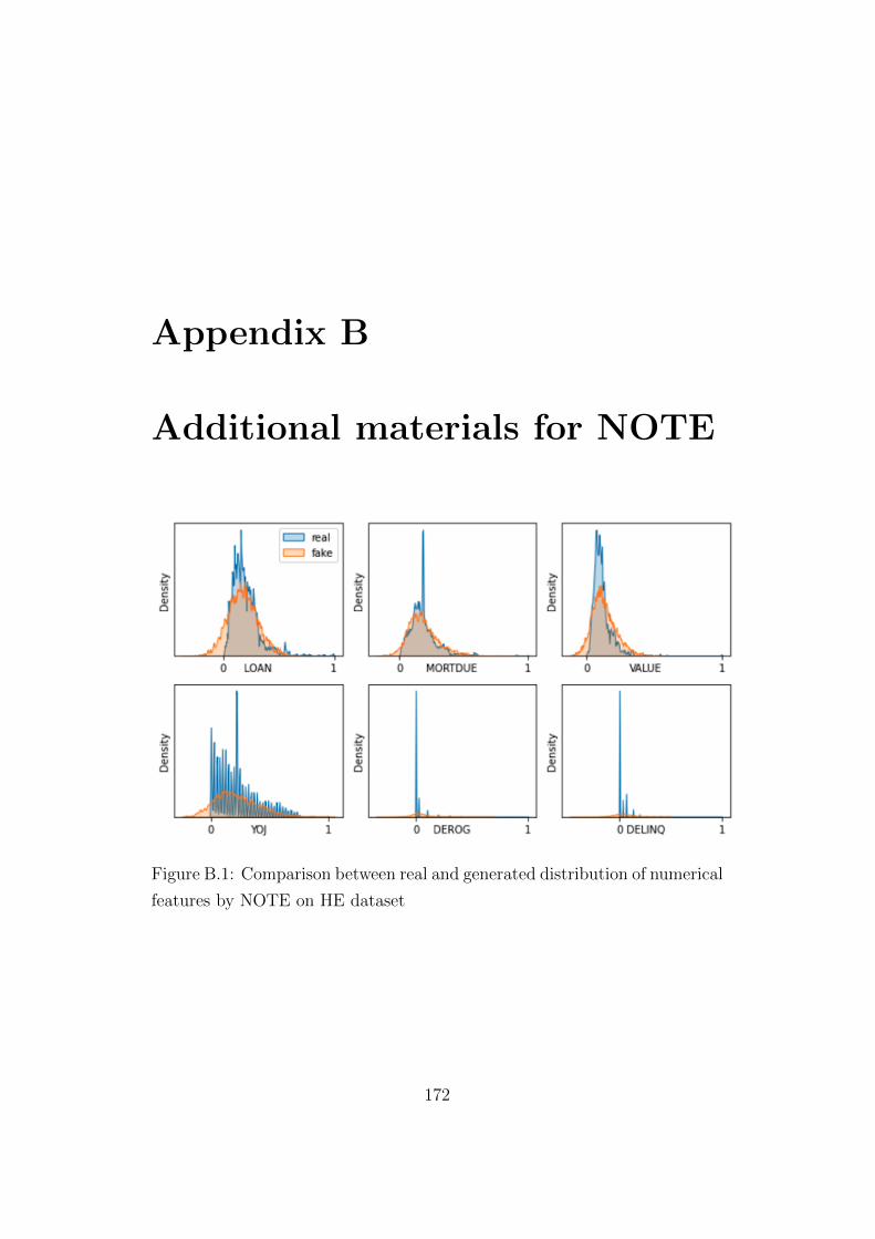
Appendix B
Additional materials for NOTE
Figure B.1: Comparison between real and generated distribution of numerical
features by NOTE on HE dataset
172

Figure B.2: The loss of generator and discriminator in NOTE (cWGAN) on
HE dataset
173

Figure B.3: The loss of generator and discriminator in GAN on HE dataset
174

Bibliography
Abdou, H., Pointon, J., and El-Masry, A. (2008). Neural nets versus con-
ventional techniques in credit scoring in egyptian banking. Expert Systems
with Applications, 35(3):1275–1292.
Acuna, E. and Rodriguez, C. (2004). The treatment of missing values and its
effect on classifier accuracy. In Classification, clustering, and data mining
applications, pages 639–647. Springer.
Akkoc, S. (2012). An empirical comparison of conventional techniques, neural
networks and the three stage hybrid adaptive neuro fuzzy inference system
(anfis) model for credit scoring analysis: The case of turkish credit card
data. European Journal of Operational Research, 222(1):168–178.
Al-Sawwa, J. and Ludwig, S. A. (2020). Performance evaluation of a cost-
sensitive differential evolution classifier using spark–imbalanced binary
classification. Journal of Computational Science, 40:101065.
Ala’raj, M. and Abbod, M. F. (2016a). Classifiers consensus system approach
for credit scoring. Knowledge-Based Systems, 104:89–105.
Ala’raj, M. and Abbod, M. F. (2016b). A new hybrid ensemble credit scoring
model based on classifiers consensus system approach. Expert Systems with
Applications, 64:36–55.
Anderson, R. (2007). The credit scoring toolkit: theory and practice for retail
credit risk management and decision automation. Oxford University Press.
175

Angelini, E., di Tollo, G., and Roli, A. (2008). A neural network approach
for credit risk evaluation. The quarterly review of economics and finance,
48(4):733–755.
Arjovsky, M., Chintala, S., and Bottou, L. (2017). Wasserstein generative
adversarial networks. In International conference on machine learning,
pages 214–223. PMLR.
Atiya, A. F. (2001). Bankruptcy prediction for credit risk using neural net-
works: A survey and new results. IEEE Transactions on neural networks,
12(4):929–935.
Awan, S. E., Bennamoun, M., Sohel, F., Sanfilippo, F., and Dwivedi, G.
(2021). Imputation of missing data with class imbalance using conditional
generative adversarial networks. Neurocomputing, 453:164–171.
Awan, S. E., Bennamoun, M., Sohel, F., Sanfilippo, F. M., and Dwivedi, G.
(2020). Imputation of missing data with class imbalance using conditional
generative adversarial networks. arXiv preprint arXiv:2012.00220.
Baesens, B., Mues, C., Martens, D., and Vanthienen, J. (2009). 50 years
of data mining and or: upcoming trends and challenges. Journal of the
Operational Research Society, 60(sup1):S16–S23.
Baesens, B., Roesch, D., and Scheule, H. (2016). Credit risk analytics: Mea-
surement techniques, applications, and examples in SAS. John Wiley &
Sons.
Baesens, B., Van Gestel, T., Viaene, S., Stepanova, M., Suykens, J., and Van-
thienen, J. (2003). Benchmarking state-of-the-art classification algorithms
for credit scoring. Journal of the operational research society, 54(6):627–
635.
Baraldi, A. N. and Enders, C. K. (2010). An introduction to modern missing
data analyses. Journal of school psychology, 48(1):5–37.
176

Basel, I. (2004). International convergence of capital measurement and cap-
ital standards: a revised framework. Bank for international settlements.
Batista, G. E., Prati, R. C., and Monard, M. C. (2004). A study of the
behavior of several methods for balancing machine learning training data.
ACM SIGKDD explorations newsletter, 6(1):20–29.
Bazarbash, M. (2019). Fintech in financial inclusion: machine learning ap-
plications in assessing credit risk. International Monetary Fund.
Beam, A. L. and Kohane, I. S. (2018). Big data and machine learning in
health care. Jama, 319(13):1317–1318.
Bengio, Y., Courville, A., and Vincent, P. (2013). Representation learning:
A review and new perspectives. IEEE transactions on pattern analysis and
machine intelligence, 35(8):1798–1828.
Bertsimas, D., Pawlowski, C., and Zhuo, Y. D. (2017). From predictive meth-
ods to missing data imputation: an optimization approach. The Journal
of Machine Learning Research, 18(1):7133–7171.
Bhattacharyya, S. and Maulik, U. (2013). Soft computing for image and
multimedia data processing. Springer.
Biau, G. (2012). Analysis of a random forests model. The Journal of Machine
Learning Research, 13(1):1063–1095.
Bijak, K. and Thomas, L. C. (2012). Does segmentation always improve
model performance in credit scoring? Expert Systems with Applications,
39(3):2433–2442.
Board, F. S. (2017). Artificial intelligence and machine learning in financial
services: Market developments and financial stability implications. Finan-
cial Stability Board, page 45.
Boughaci, D. and Alkhawaldeh, A. A. (2020). Appropriate machine learning
techniques for credit scoring and bankruptcy prediction in banking and
177

finance: A comparative study. Risk and Decision Analysis, (Preprint):1–
10.
Breiman, L. (1996). Bagging predictors. Machine learning, 24(2):123–140.
Breiman, L. (2001). Random forests. Machine learning, 45(1):5–32.
Breiman, L., Friedman, J., Stone, C. J., and Olshen, R. A. (1984). Classifi-
cation and regression trees. CRC press.
Brown, I. and Mues, C. (2012). An experimental comparison of classification
algorithms for imbalanced credit scoring data sets. Expert Systems with
Applications, 39(3):3446–3453.
Burez, J. and Van den Poel, D. (2009). Handling class imbalance in customer
churn prediction. Expert Systems with Applications, 36(3):4626–4636.
Bussmann, N., Giudici, P., Marinelli, D., and Papenbrock, J. (2021). Ex-
plainable machine learning in credit risk management. Computational
Economics, 57(1):203–216.
Buuren, S. v. and Groothuis-Oudshoorn, K. (2010). mice: Multivariate im-
putation by chained equations in r. Journal of statistical software, pages
1–68.
Camino, R. D., Hammerschmidt, C. A., and State, R. (2019). Improving
missing data imputation with deep generative models. arXiv preprint
arXiv:1902.10666.
Carey, M. and Hrycay, M. (2001). Parameterizing credit risk models with
rating data. Journal of banking & finance, 25(1):197–270.
Chawla, N. V., Bowyer, K. W., Hall, L. O., and Kegelmeyer, W. P. (2002).
Smote: synthetic minority over-sampling technique. Journal of artificial
intelligence research, 16:321–357.
Cheema, J. R. (2014). A review of missing data handling methods in educa-
tion research. Review of Educational Research, 84(4):487–508.
178

Chen, N., Ribeiro, B., and Chen, A. (2016). Financial credit risk assessment:
a recent review. Artificial Intelligence Review, 45(1):1–23.
Chen, T. and Guestrin, C. (2016). Xgboost: A scalable tree boosting sys-
tem. In Proceedings of the 22nd acm sigkdd international conference on
knowledge discovery and data mining, pages 785–794.
Choi, E., Biswal, S., Malin, B., Duke, J., Stewart, W. F., and Sun, J. (2017).
Generating multi-label discrete patient records using generative adversarial
networks. In Machine learning for healthcare conference, pages 286–305.
PMLR.
Cox, D. R. (1958). The regression analysis of binary sequences. Journal of
the Royal Statistical Society: Series B (Methodological), 20(2):215–232.
Croxson, K., Bracke, P., and Jung, C. (2019). Explaining why the computer
says ‘no’. FCA, 5:31.
Dastile, X., Celik, T., and Potsane, M. (2020). Statistical and machine
learning models in credit scoring: A systematic literature survey. Applied
Soft Computing, 91:106263.
Dempster, A. P., Laird, N. M., and Rubin, D. B. (1977). Maximum likelihood
from incomplete data via the em algorithm. Journal of the Royal Statistical
Society: Series B (Methodological), 39(1):1–22.
Dietterich, T. G. (2000). An experimental comparison of three methods for
constructing ensembles of decision trees: Bagging, boosting, and random-
ization. Machine learning, 40(2):139–157.
Donders, A. R. T., Van Der Heijden, G. J., Stijnen, T., and Moons, K. G.
(2006). A gentle introduction to imputation of missing values. Journal of
clinical epidemiology, 59(10):1087–1091.
Dong, W., Fong, D. Y. T., Yoon, J.-s., Wan, E. Y. F., Bedford, L. E., Tang,
E. H. M., and Lam, C. L. K. (2021). Generative adversarial networks for
179

imputing missing data for big data clinical research. BMC medical research
methodology, 21(1):1–10.
Douzas, G. and Bacao, F. (2018). Effective data generation for imbalanced
learning using conditional generative adversarial networks. Expert Systems
with applications, 91:464–471.
Drummond, C. and Holte, R. C. (2005). Severe class imbalance: Why bet-
ter algorithms aren’t the answer. In European Conference on Machine
Learning, pages 539–546. Springer.
Dua, D., Graff, C., et al. (2017). Uci machine learning repository.
Duin, R. P. and Tax, D. M. (2000). Experiments with classifier combining
rules. In International Workshop on Multiple Classifier Systems, pages
16–29. Springer.
Ebenuwa, S. H., Sharif, M. S., Alazab, M., and Al-Nemrat, A. (2019). Vari-
ance ranking attributes selection techniques for binary classification prob-
lem in imbalance data. IEEE Access, 7:24649–24666.
Enders, C. K. and Gottschall, A. C. (2011). Multiple imputation strategies for
multiple group structural equation models. Structural Equation Modeling,
18(1):35–54.
Engelmann, J. and Lessmann, S. (2021). Conditional wasserstein gan-based
oversampling of tabular data for imbalanced learning. Expert Systems with
Applications, 174:114582.
Erichson, N. B., Mathelin, L., Kutz, J. N., and Brunton, S. L. (2019a). Ran-
domized dynamic mode decomposition. SIAM Journal on Applied Dynam-
ical Systems, 18(4):1867–1891.
Erichson, N. B., Voronin, S., Brunton, S. L., and Kutz, J. N. (2019b). Ran-
domized matrix decompositions using r. Journal of Statistical Software,
89(1):1–48.
180

Erichson, N. B., Voronin, S., Brunton, S. L., and Kutz, J. N. (2019c). Ran-
domized matrix decompositions using r. Journal of Statistical Software,
89(1):1–48.
Falangis, K. and Glen, J. (2010). Heuristics for feature selection in mathemat-
ical programming discriminant analysis models. Journal of the Operational
Research Society, 61(5):804–812.
Fawcett, T. (2004). Roc graphs: Notes and practical considerations for re-
searchers. Machine learning, 31(1):1–38.
Fawcett, T. (2006). An introduction to roc analysis. Pattern recognition
letters, 27(8):861–874.
Finlay, S. (2011). Multiple classifier architectures and their application
to credit risk assessment. European Journal of Operational Research,
210(2):368–378.
Fiore, U., De Santis, A., Perla, F., Zanetti, P., and Palmieri, F. (2019). Using
generative adversarial networks for improving classification effectiveness in
credit card fraud detection. Information Sciences, 479:448–455.
Fisher, R. A. (1936). The use of multiple measurements in taxonomic prob-
lems. Annals of eugenics, 7(2):179–188.
Florez-Lopez, R. (2010). Effects of missing data in credit risk scoring. a
comparative analysis of methods to achieve robustness in the absence of
sufficient data. Journal of the Operational Research Society, 61(3):486–501.
Florez-Lopez, R. and Ramon-Jeronimo, J. M. (2015). Enhancing accuracy
and interpretability of ensemble strategies in credit risk assessment. a
correlated-adjusted decision forest proposal. Expert Systems with Applica-
tions, 42(13):5737–5753.
Friedman, J. H. (2001). Greedy function approximation: a gradient boosting
machine. Annals of statistics, pages 1189–1232.
181

Fu, K., Cheng, D., Tu, Y., and Zhang, L. (2016). Credit card fraud detec-
tion using convolutional neural networks. In International Conference on
Neural Information Processing, pages 483–490. Springer.
Garcıa, V., Marques, A., and Sanchez, J. S. (2012). On the use of data
filtering techniques for credit risk prediction with instance-based models.
Expert Systems with Applications, 39(18):13267–13276.
Garcıa, V., Marques, A. I., and Sanchez, J. S. (2015). An insight into the
experimental design for credit risk and corporate bankruptcy prediction
systems. Journal of Intelligent Information Systems, 44(1):159–189.
Garcıa-Laencina, P. J., Sancho-Gomez, J.-L., and Figueiras-Vidal, A. R.
(2010). Pattern classification with missing data: a review. Neural Com-
puting and Applications, 19(2):263–282.
Geurts, P., Ernst, D., and Wehenkel, L. (2006). Extremely randomized trees.
Machine learning, 63(1):3–42.
Goodfellow, I., Pouget-Abadie, J., Mirza, M., Xu, B., Warde-Farley, D.,
Ozair, S., Courville, A., and Bengio, Y. (2014). Generative adversarial
nets. Advances in neural information processing systems, 27:2672–2680.
Guyon, I. and Elisseeff, A. (2003). An introduction to variable and feature
selection. Journal of machine learning research, 3(Mar):1157–1182.
Haixiang, G., Yijing, L., Shang, J., Mingyun, G., Yuanyue, H., and Bing,
G. (2017). Learning from class-imbalanced data: Review of methods and
applications. Expert Systems with Applications, 73:220–239.
Halmich, C. (2020). WGAIN: Data Imputation using Wasserstein GAIN.
PhD thesis, Universitat Linz.
Hammad Alharbi, H. and Kimura, M. (2020). Missing data imputation us-
ing data generated by gan. In 2020 the 3rd International Conference on
Computing and Big Data, pages 73–77.
182

Hamori, S., Kawai, M., Kume, T., Murakami, Y., and Watanabe, C. (2018).
Ensemble learning or deep learning? application to default risk analysis.
Journal of Risk and Financial Management, 11(1):12.
Han, H., Wang, W.-Y., and Mao, B.-H. (2005). Borderline-smote: a new
over-sampling method in imbalanced data sets learning. In International
conference on intelligent computing, pages 878–887. Springer.
Hand, D. and Zhou, F. (2010). Evaluating models for classifying customers
in retail banking collections. Journal of the Operational Research Society,
61(10):1540–1547.
Hand, D. J. and Henley, W. E. (1997). Statistical classification methods in
consumer credit scoring: a review. Journal of the Royal Statistical Society:
Series A (Statistics in Society), 160(3):523–541.
Hastie, T., Tibshirani, R., and Friedman, J. (2009). The elements of statis-
tical learning: data mining, inference, and prediction. pages 337–387.
He, C., Ma, M., and Wang, P. (2020). Extract interpretability-accuracy
balanced rules from artificial neural networks: A review. Neurocomputing,
387:346–358.
He, H., Bai, Y., Garcia, E. A., and Li, S. (2008). Adasyn: Adaptive synthetic
sampling approach for imbalanced learning. In 2008 IEEE international
joint conference on neural networks (IEEE world congress on computa-
tional intelligence), pages 1322–1328. IEEE.
He, H., Zhang, W., and Zhang, S. (2018). A novel ensemble method for
credit scoring: Adaption of different imbalance ratios. Expert Systems
with Applications, 98:105–117.
Henley, W. and Hand, D. J. (1996). Ak-nearest-neighbour classifier for assess-
ing consumer credit risk. Journal of the Royal Statistical Society: Series
D (The Statistician), 45(1):77–95.
183

Hinton, G. E. and Salakhutdinov, R. R. (2006). Reducing the dimensionality
of data with neural networks. science, 313(5786):504–507.
Honaker, J., King, G., Blackwell, M., et al. (2011). Amelia ii: A program for
missing data. Journal of statistical software, 45(7):1–47.
Horton, N. J. and Kleinman, K. P. (2007). Much ado about nothing: A
comparison of missing data methods and software to fit incomplete data
regression models. The American Statistician, 61(1):79–90.
Hu, S., Liang, Y., Ma, L., and He, Y. (2009). Msmote: Improving classi-
fication performance when training data is imbalanced. In 2009 second
international workshop on computer science and engineering, volume 2,
pages 13–17. IEEE.
Huang, J. and Ling, C. X. (2005). Using auc and accuracy in evaluating learn-
ing algorithms. IEEE Transactions on knowledge and Data Engineering,
17(3):299–310.
Huang, Z., Chen, H., Hsu, C.-J., Chen, W.-H., and Wu, S. (2004). Credit rat-
ing analysis with support vector machines and neural networks: a market
comparative study. Decision support systems, 37(4):543–558.
Ibrahim, J. G., Chen, M.-H., Lipsitz, S. R., and Herring, A. H. (2005).
Missing-data methods for generalized linear models: A comparative review.
Journal of the American Statistical Association, 100(469):332–346.
Jagtiani, J. and Lemieux, C. (2017). Fintech lending: Financial inclusion,
risk pricing, and alternative information.
Jain, A. K., Mao, J., and Mohiuddin, K. M. (1996). Artificial neural net-
works: A tutorial. Computer, 29(3):31–44.
Japkowicz, N. (2000). The class imbalance problem: Significance and strate-
gies. In Proc. of the Int’l Conf. on Artificial Intelligence, volume 56. Cite-
seer.
184

Jerez, J. M., Molina, I., Garcıa-Laencina, P. J., Alba, E., Ribelles, N., Martın,
M., and Franco, L. (2010). Missing data imputation using statistical and
machine learning methods in a real breast cancer problem. Artificial in-
telligence in medicine, 50(2):105–115.
Jiang, Y. (2009). Credit scoring model based on the decision tree and the
simulated annealing algorithm. In 2009 WRI World Congress on Computer
Science and Information Engineering, volume 4, pages 18–22. IEEE.
Jolliffe, I. T. (1986). Principal components in regression analysis. In Principal
component analysis, pages 129–155. Springer.
Jordan, M. I. and Mitchell, T. M. (2015). Machine learning: Trends, per-
spectives, and prospects. Science, 349(6245):255–260.
Kennedy, K. (2013). Credit scoring using machine learning. PhD thesis,
Dublin Institute of Technology.
Khoshgoftaar, T. M., Seiffert, C., Van Hulse, J., Napolitano, A., and Folleco,
A. (2007). Learning with limited minority class data. In Sixth International
Conference on Machine Learning and Applications (ICMLA 2007), pages
348–353. IEEE.
Kim, Y. S. and Sohn, S. Y. (2004). Managing loan customers using misclassi-
fication patterns of credit scoring model. Expert Systems with Applications,
26(4):567–573.
Kline, R. B. (2015). Principles and practice of structural equation modeling.
Guilford publications.
Kotsiantis, S., Kanellopoulos, D., and Tampakas, V. (2006). On implement-
ing a financial decision support system. International Journal of Computer
Science and Network Security, 6(1a):103–112.
Kullback, S. and Leibler, R. A. (1951). On information and sufficiency. The
annals of mathematical statistics, 22(1):79–86.
185

Kumar, P. R. and Ravi, V. (2007). Bankruptcy prediction in banks and
firms via statistical and intelligent techniques–a review. European journal
of operational research, 180(1):1–28.
Lee, T.-S. and Chen, I.-F. (2005). A two-stage hybrid credit scoring model us-
ing artificial neural networks and multivariate adaptive regression splines.
Expert Systems with Applications, 28(4):743–752.
Lee, T.-S., Chiu, C.-C., Chou, Y.-C., and Lu, C.-J. (2006). Mining the
customer credit using classification and regression tree and multivariate
adaptive regression splines. Computational Statistics & Data Analysis,
50(4):1113–1130.
Lessmann, S., Baesens, B., Seow, H.-V., and Thomas, L. C. (2015). Bench-
marking state-of-the-art classification algorithms for credit scoring: An
update of research. European Journal of Operational Research, 247(1):124–
136.
Li, C., Zhu, J., and Zhang, B. (2017). Max-margin deep generative models
for (semi-) supervised learning. IEEE transactions on pattern analysis and
machine intelligence, 40(11):2762–2775.
Li, P., Stuart, E. A., and Allison, D. B. (2015). Multiple imputation: a
flexible tool for handling missing data. Jama, 314(18):1966–1967.
Liang, D., Tsai, C.-F., and Wu, H.-T. (2015). The effect of feature selection
on financial distress prediction. Knowledge-Based Systems, 73:289–297.
Lin, J. (1991). Divergence measures based on the shannon entropy. IEEE
Transactions on Information theory, 37(1):145–151.
Lin, W.-Y., Hu, Y.-H., and Tsai, C.-F. (2011). Machine learning in financial
crisis prediction: a survey. IEEE Transactions on Systems, Man, and
Cybernetics, Part C (Applications and Reviews), 42(4):421–436.
Little, R. J. and Rubin, D. B. (1989). The analysis of social science data
with missing values. Sociological Methods & Research, 18(2-3):292–326.
186

Little, R. J. and Rubin, D. B. (2019). Statistical analysis with missing data,
volume 793. John Wiley & Sons.
Liu, Y. and Schumann, M. (2005). Data mining feature selection for credit
scoring models. Journal of the Operational Research Society, 56(9):1099–
1108.
Longadge, R. and Dongre, S. (2013). Class imbalance problem in data mining
review. arXiv e-prints, pages arXiv–1305.
Lundberg, S. M., Erion, G., Chen, H., DeGrave, A., Prutkin, J. M., Nair,
B., Katz, R., Himmelfarb, J., Bansal, N., and Lee, S.-I. (2020). From local
explanations to global understanding with explainable ai for trees. Nature
machine intelligence, 2(1):56–67.
Lundberg, S. M. and Lee, S.-I. (2017). A unified approach to interpreting
model predictions. Advances in Neural Information Processing Systems,
30:4765–4774.
Lyn, T., David, E. B., and Jonathan, C. N. (2002). Credit scoring and its
applications. Philadelphia: Society for Industrial and Applied Mathemat-
ics.
Makowski, P. (1985). Credit scoring branches out. Credit World, 75(1):30–37.
Mani, I. and Zhang, I. (2003). knn approach to unbalanced data distributions:
a case study involving information extraction. In Proceedings of workshop
on learning from imbalanced datasets, volume 126.
Mansour, Y. (1997). Pessimistic decision tree pruning based on tree
size. In MACHINE LEARNING-INTERNATIONAL WORKSHOP THEN
CONFERENCE-, pages 195–201. Citeseer.
Marques, A. I., Garcıa, V., and Sanchez, J. S. (2012). Exploring the be-
haviour of base classifiers in credit scoring ensembles. Expert Systems with
Applications, 39(11):10244–10250.
187

Marques, A. I., Garcıa, V., and Sanchez, J. S. (2013). On the suitability of
resampling techniques for the class imbalance problem in credit scoring.
Journal of the Operational Research Society, 64(7):1060–1070.
McCarthy, J., Minsky, M. L., Rochester, N., and Shannon, C. E. (2006). A
proposal for the dartmouth summer research project on artificial intelli-
gence, august 31, 1955. AI magazine, 27(4):12–12.
McKnight, P. E., McKnight, K. M., Sidani, S., and Figueredo, A. J. (2007).
Missing data: A gentle introduction. Guilford Press.
Mirza, M. and Osindero, S. (2014). Conditional generative adversarial nets.
arXiv preprint arXiv:1411.1784.
Mitchell, T. M. et al. (1997). Machine learning. 1997. Burr Ridge, IL:
McGraw Hill, 45(37):870–877.
Muller, K.-R., Mika, S., Tsuda, K., and Scholkopf, K. (2018). An intro-
duction to kernel-based learning algorithms. Handbook of Neural Network
Signal Processing, pages 4–1.
Munkhdalai, L., Munkhdalai, T., Namsrai, O.-E., Lee, J. Y., and Ryu, K. H.
(2019). An empirical comparison of machine-learning methods on bank
client credit assessments. Sustainability, 11(3):699.
Murdoch, W. J., Singh, C., Kumbier, K., Abbasi-Asl, R., and Yu, B. (2019).
Definitions, methods, and applications in interpretable machine learning.
Proceedings of the National Academy of Sciences, 116(44):22071–22080.
Myung, I. J. (2003). Tutorial on maximum likelihood estimation. Journal of
mathematical Psychology, 47(1):90–100.
Nanni, L. and Lumini, A. (2009). An experimental comparison of ensemble
of classifiers for bankruptcy prediction and credit scoring. Expert systems
with applications, 36(2):3028–3033.
188

Nascimento, D. S., Coelho, A. L., and Canuto, A. M. (2014). Integrating
complementary techniques for promoting diversity in classifier ensembles:
A systematic study. Neurocomputing, 138:347–357.
Nationalbank, O. (2004). Guidelines on credit risk management: Rating
models and validation. Oesterreichische Nationalbank.
Nazabal, A., Olmos, P. M., Ghahramani, Z., and Valera, I. (2020). Han-
dling incomplete heterogeneous data using vaes. Pattern Recognition,
107:107501.
Neagoe, V.-E., Ciotec, A.-D., and Cucu, G.-S. (2018). Deep convolutional
neural networks versus multilayer perceptron for financial prediction. In
2018 International Conference on Communications (COMM), pages 201–
206. IEEE.
Ong, C.-S., Huang, J.-J., and Tzeng, G.-H. (2005). Building credit scoring
models using genetic programming. Expert Systems with Applications,
29(1):41–47.
Paleologo, G., Elisseeff, A., and Antonini, G. (2010). Subagging for credit
scoring models. European journal of operational research, 201(2):490–499.
Quinlan, J. R. (1986). Induction of decision trees. Machine learning, 1(1):81–
106.
Ratner, B. (2017). Statistical and Machine-Learning Data Mining:: Tech-
niques for Better Predictive Modeling and Analysis of Big Data. CRC
Press.
Ravanbakhsh, M., Nabi, M., Sangineto, E., Marcenaro, L., Regazzoni, C.,
and Sebe, N. (2017). Abnormal event detection in videos using genera-
tive adversarial nets. In 2017 IEEE International Conference on Image
Processing (ICIP), pages 1577–1581. IEEE.
Rish, I. et al. (2001). An empirical study of the naive bayes classifier. In
IJCAI 2001 workshop on empirical methods in artificial intelligence, vol-
ume 3, pages 41–46.
189

Roderick, J., Little, A., and Rubin, D. B. (2002). Statistical analysis with
missing data.
Royston, P., White, I. R., et al. (2011). Multiple imputation by chained
equations (mice): implementation in stata. J Stat Softw, 45(4):1–20.
Rubin, D. B. (1976). Inference and missing data. Biometrika, 63(3):581–592.
Ruiz-Chavez, Z., Salvador-Meneses, J., and Garcia-Rodriguez, J. (2018). Ma-
chine learning methods based preprocessing to improve categorical data
classification. In International Conference on Intelligent Data Engineering
and Automated Learning, pages 297–304. Springer.
Russell, S. and Norvig, P. (2002). Artificial intelligence: a modern approach.
Salgado, C. M., Azevedo, C., Proenca, H., and Vieira, S. M. (2016). Missing
data. Secondary analysis of electronic health records, pages 143–162.
Schafer, J. L. (1997). Analysis of incomplete multivariate data. CRC press.
Schapire, R. E. (1990). The strength of weak learnability. Machine learning,
5(2):197–227.
Schlegl, T., Seebock, P., Waldstein, S. M., Schmidt-Erfurth, U., and Langs,
G. (2017). Unsupervised anomaly detection with generative adversarial
networks to guide marker discovery. In International conference on infor-
mation processing in medical imaging, pages 146–157. Springer.
Seaman, S. R., Bartlett, J. W., and White, I. R. (2012). Multiple imputation
of missing covariates with non-linear effects and interactions: an evaluation
of statistical methods. BMC medical research methodology, 12(1):1–13.
Seo, S., Jeon, Y., and Kim, J. (2018). Meta learning for imbalanced big data
analysis by using generative adversarial networks. In Proceedings of the
2018 International Conference on Big Data and Computing, pages 5–9.
Shah, A. D., Bartlett, J. W., Carpenter, J., Nicholas, O., and Hemingway, H.
(2014). Comparison of random forest and parametric imputation models
190

for imputing missing data using mice: a caliber study. American journal
of epidemiology, 179(6):764–774.
Shapley, L. S. (1953). A value for n-person games. Contributions to the
Theory of Games, 2(28):307–317.
Siddiqi, N. (2012). Credit risk scorecards: developing and implementing in-
telligent credit scoring, volume 3. John Wiley & Sons.
Sirignano, J., Sadhwani, A., and Giesecke, K. (2016). Deep learning for
mortgage risk. arXiv preprint arXiv:1607.02470.
Smieja, M., Struski, L., Tabor, J., Zielinski, B., and Spurek, P.
(2018). Processing of missing data by neural networks. arXiv preprint
arXiv:1805.07405.
Son, M., Jung, S., Moon, J., and Hwang, E. (2020). Bcgan-based over-
sampling scheme for imbalanced data. In 2020 IEEE International Con-
ference on Big Data and Smart Computing (BigComp), pages 155–160.
IEEE.
Srivastava, A., Valkoz, L., Russell, C., Gutmann, M., and Sutton, C. (2017).
Veegan: Reducing mode collapse in gans using implicit variational learn-
ing. Advances in Neural Information Processing Systems 30 (NIPS 2017)
pre-proceedings, 30.
Stekhoven, D. J. and Buhlmann, P. (2012). Missforest—non-parametric miss-
ing value imputation for mixed-type data. Bioinformatics, 28(1):112–118.
Sustersic, M., Mramor, D., and Zupan, J. (2009). Consumer credit scoring
models with limited data. Expert Systems with Applications, 36(3):4736–
4744.
Thomas, L. C. (2000). A survey of credit and behavioural scoring: forecasting
financial risk of lending to consumers. International journal of forecasting,
16(2):149–172.
191

Thomas, L. C., Oliver, R. W., and Hand, D. J. (2005). A survey of the
issues in consumer credit modelling research. Journal of the Operational
Research Society, 56(9):1006–1015.
Troyanskaya, O., Cantor, M., Sherlock, G., Brown, P., Hastie, T., Tibshirani,
R., Botstein, D., and Altman, R. B. (2001). Missing value estimation
methods for dna microarrays. Bioinformatics, 17(6):520–525.
Valera, I. and Ghahramani, Z. (2017). Automatic discovery of the statistical
types of variables in a dataset. In International Conference on Machine
Learning, pages 3521–3529. PMLR.
Van der Maaten, L. and Hinton, G. (2008). Visualizing data using t-sne.
Journal of machine learning research, 9(11).
Vriens, M. and Melton, E. (2002). Managing missing data. Marketing Re-
search, 14(3):12.
Wang, G., Hao, J., Ma, J., and Jiang, H. (2011). A comparative assessment
of ensemble learning for credit scoring. Expert systems with applications,
38(1):223–230.
Wang, G., Ma, J., Huang, L., and Xu, K. (2012). Two credit scoring models
based on dual strategy ensemble trees. Knowledge-Based Systems, 26:61–
68.
West, D. (2000). Neural network credit scoring models. Computers & Oper-
ations Research, 27(11-12):1131–1152.
Wolpert, D. H. and Macready, W. G. (1997). No free lunch theorems for
optimization. IEEE transactions on evolutionary computation, 1(1):67–
82.
Worth, A. P. and Cronin, M. T. (2003). The use of discriminant analy-
sis, logistic regression and classification tree analysis in the development
of classification models for human health effects. Journal of Molecular
Structure: THEOCHEM, 622(1-2):97–111.
192

Xia, Y., Liu, C., Da, B., and Xie, F. (2018). A novel heterogeneous ensemble
credit scoring model based on bstacking approach. Expert Systems with
Applications, 93:182–199.
Xia, Y., Liu, C., Li, Y., and Liu, N. (2017). A boosted decision tree approach
using bayesian hyper-parameter optimization for credit scoring. Expert
Systems with Applications, 78:225–241.
Xiao, H., Xiao, Z., and Wang, Y. (2016). Ensemble classification based on
supervised clustering for credit scoring. Applied Soft Computing, 43:73–86.
Xu, L., Skoularidou, M., Cuesta-Infante, A., and Veeramachaneni, K. (2019).
Modeling tabular data using conditional gan. Advances in Neural Infor-
mation Processing Systems, 32:7335–7345.
Xu, L. and Veeramachaneni, K. (2018). Synthesizing tabular data using
generative adversarial networks. arXiv e-prints, pages arXiv–1811.
Yeh, C.-C., Lin, F., and Hsu, C.-Y. (2012). A hybrid kmv model, random
forests and rough set theory approach for credit rating. Knowledge-Based
Systems, 33:166–172.
Yeh, I.-C. and Lien, C.-h. (2009). The comparisons of data mining techniques
for the predictive accuracy of probability of default of credit card clients.
Expert Systems with Applications, 36(2):2473–2480.
Yeh, S.-H., Wang, C.-J., and Tsai, M.-F. (2015). Deep belief networks for
predicting corporate defaults. In 2015 24th Wireless and Optical Commu-
nication Conference (WOCC), pages 159–163. IEEE.
Yoon, J., Jordon, J., and Schaar, M. (2018). Gain: Missing data imputation
using generative adversarial nets. In International Conference on Machine
Learning, pages 5689–5698. PMLR.
Yuan, Y. C. (2010). Multiple imputation for missing data: Concepts and new
development (version 9.0). SAS Institute Inc, Rockville, MD, 49(1-11):12.
193

Zentralbank, E. (2004). credit risk transfer by eu banks: activities, risks and
risk management “. European Central Bank Report, Frankfurt am Main.
Zhang, G., Wang, X., Li, R., Song, Y., He, J., and Lai, J. (2020). Network
intrusion detection based on conditional wasserstein generative adversarial
network and cost-sensitive stacked autoencoder. IEEE Access, 8:190431–
190447.
Zheng, M., Li, T., Zhu, R., Tang, Y., Tang, M., Lin, L., and Ma, Z. (2020).
Conditional wasserstein generative adversarial network-gradient penalty-
based approach to alleviating imbalanced data classification. Information
Sciences, 512:1009–1023.
Zieba, M., Tomczak, S. K., and Tomczak, J. M. (2016). Ensemble boosted
trees with synthetic features generation in application to bankruptcy pre-
diction. Expert Systems with Applications, 58:93–101.
194


