Explicit versus Implicit Contracts for Dividing the Benefits of Cooperation*

Marco Casari and Timothy N. Cason

Purdue University

December 2007

Abstract

Explicit contracts are used most frequently by theorists to model many relationships, ranging from labor markets to investment projects. Experimental evidence has accumulated recently highlighting the limitations of formal and explicit contracts in certain situations, and has documented environments in which informal and implicit contracts are more efficient. This paper compares the performance of explicit and implicit contracts in a new partnership environment in which both contracting parties must incur effort to generate a joint surplus, and one (“strong”) agent controls the surplus division. In the treatment in which the strong agent makes a non-binding “bonus” offer to the weak agent, this unenforceable promise doubles the rate of joint high effort compared to a baseline with no promise. The strong agents most frequently offered a bonus to split the gains of the high effort equally, but actually delivered this bonus amount only about one-quarter of the time. An explicit and enforceable contract offer performs substantially better, raising the rate of the most efficient outcome by over 200 percent relative to the baseline. Interestingly, the initial bonus offer helped agents to coordinate their effort choices.

Keywords: Trust, contracting, laboratory, experiments, social preferences, inequity aversion, reciprocity *casari@purdue.edu; cason@purdue.edu; Mailing address: Krannert School of Management, Purdue University, West Lafayette, IN 47907-2076, U.S.A. Fax: +1-765-494-9658. Funding for subject payments was provided by the Purdue University Faculty Scholar program. We thank Sukanya Chaudhuri and Jingjing Zhang for research assistance. Helpful comments on earlier versions of this work were provided by Dirk Engelmann, Dan Kovenock, and presentation audiences at the Barcelona ISNIE conference, Purdue University, IUPUI, and ESA conferences in Rome and Tucson.

1

1. Introduction

Contract theory has been developed mostly on the domain of self-regarding preferences. While

this focus has allowed researchers to address important questions in optimal contract design and

other areas, the emphasis on explicit incentive contracts has been challenged in the last decade

by accumulating laboratory evidence on “fair-minded” agents. For example, in a laboratory labor

market Fehr et al. (2007) show that unenforceable bonus contracts can outperform explicit

incentive contracts when agents have preferences for fairness. Moreover, their principals

recognize this and frequently choose the unenforceable contract when given a choice of contract

format.

General results in contract theory could in principle be extended to many preference

structures, including those based on fairness. The challenging empirical results generated in the

laboratory necessarily must focus on special cases, and so before undertaking such extensions it

is important to explore a variety of environments to identify where explicit contracts perform

worse and better than implicit contracts. Ben-Ner and Putterman (2007) show that implicit

contracts in a simple trust game are effective and preferred by subjects over costly explicit

contracts when pre-play communication is possible. By contrast, implicit gift exchange contracts

are apparently less effective when effort is more costly and not individually observable by the

experimenter (Rigdon, 2002), when payoffs are presented differently (Charness et al., 2004), or

for different parametrizations (Fehr et al., 2007; Healy, forthcoming). Other research has found

that implicit gift exchange contracts that work well in the laboratory may have only a temporary

impact on behavior in longer field experiments (Gneezy and List, 2006). The present study’s

objective is to compare the performance of explicit and implicit contracts in a new alternative

economic environment.

As in most of the extensive literature on experimental labor markets (for a review, see

Gächter and Fehr, 2001, or Frey and Osterloh, 2002), in our experiment two agents must

cooperate to generate some joint surplus that is split between them. In the standard environment

the principal pays the agent and the agent exerts effort that benefits the principal. The moves are

typically sequential, although payments sometimes occur before and sometimes after the effort.

By contrast, in our experiment the two agents move simultaneously to generate some joint

surplus that they can share. Hence we call this a “partnership” game, since the agents are more

equal partners than the sequential principal-agent relationships such as Charness and

2

Dufwenberg (2006) or Fehr et al. (2007). Nevertheless, as in a labor market the environment is

also hierarchical, because one agent—call her the principal or simply the “strong agent”—is

responsible for dividing the benefits of their high effort. We examine treatments in which the

strong agent offers an unenforceable “bonus” payment to the other agent, or an explicit and

formal contract with an effort-contingent payment. The environment is also simplified in some

dimensions (e.g., only two effort choices are feasible) but is rich in others (e.g., the strong agent

can divide the surplus between the two agents in virtually any way desired).

We make no claim that this environment with simultaneous contributions to generate the

joint surplus is any better or more representative than the sequential design typically considered

in the literature. Rather, we simply observe that many profitable economic interactions, both in

the labor market and elsewhere, require efforts of multiple individuals; and that efforts are

simultaneous (from a modeling perspective) when information about others’ efforts is limited.

Examples from management contexts are common, such as many situations where work teams

collaborate on a project from multiple locations and a manager allocates a project bonus. Firms

organized as partnerships provide a good concrete example. Many such firms have senior

partners who have substantially greater power in determining annual bonuses for junior partners

and associates.

We find that in this environment, efficient high effort outcomes are feasible in theory

even without explicit contracts for some intermediate distributions of inequity averse social

preferences. Joint high effort is not an equilibrium if too many or too few agents have self-

regarding preferences. Empirically, we document that explicit contracts considerably outperform

implicit (bonus) contracts, as well as a baseline treatment with no opportunity for any kind of

contract offer.1 Although the promise of an unenforceable payment doubles the rate of joint high

effort relative to the baseline, the formal contract increases this rate by 233 percent. Effort also

decreases with experience in the baseline and bonus treatments but increases with experience in

the formal contract treatment, so these performance differences increase over time. In the Bonus

treatment, the strong agents most frequently offered to split the gains of high effort equally, but

actually delivered an equal split only about one-quarter of the time. Very low and high offers did

help agents coordinate on the low effort equilibrium, however. This is consistent with the

1 Although our subjects do not sign actual contracts in the experiment, they sometimes make fully-enforcable commitments that are analogous to explicit contracts. The subjects did not see this “contract” framing of the problem during the experiment, but we adopt it here to be consistent with the existing experimental literature.

3

interpretation that offers can signal information about different preference types, reflecting

heterogeneity across individuals’ other-regarding preferences.

The next section describes the partnership game along with the experimental design and

procedures. Section 3 presents some theoretical predictions for the benchmark case in which all

agents have standard money-maximizing preferences, as well as a simple version of inequity

averse social preferences. Section 4 contains the results and Section 5 concludes.

2. Experimental Design and Procedures

An experimental session included four parts: (1) Lotteries to measure risk attitude; (2)

Ultimatum game; (3) Trust game; (4) Partnership game.2 The main focus of this study is on the

partnership game, hence we describe it first. Before learning the results from parts 1-3, subjects

played 10 periods of the partnership game illustrated in Table 1. The special aspect was that one

agent had a “strong” role and another a “weak” role. Whenever the high effort outcome (1, 1)

was reached, the strong agent chose A and B(onus) and thus was the dictator in splitting the 60-

franc gain. Roles were common knowledge. We conduct three treatments in an across-subject

design: Baseline, Bonus and Explicit Commitment.

Table 1: The Partnership Game

Weak agent

1 (high effort) 2 (low effort)

1 (high effort) A, B

(A+B=60)

0, 10

Strong agent 2 (low effort) 10, 0 10, 10

In the Baseline treatment a strong and a weak agent made a simultaneous choice between

1 and 2. When the strong agent chose 1, she was then asked, in addition, to decide on how she

would split the 60 francs in case the outcome (1, 1) was reached. The subjects saw the results at

the end of each period. The weak agent learned nothing about the actual allocation made by the

strong agent when the outcome was (1, 2).

2 Sample instructions are available in the appendix.

4

In the Bonus treatment the strong agent first sent “a message about the allocation” to the

weak agent, “(I earn …, you earn …)” and then the procedure was the same as in the Baseline

treatment. In a second stage, both strong and weak agents made a simultaneous choice between 1

and 2. When the strong agent chose 1, she had to decide, in addition, on how she would split the

60 francs in case the outcome (1, 1) was reached. The actual split could be different from the one

promised. The subjects saw the results at the end of each period. The weak agent learned the

actual allocation choice of the strong agent only when the outcome (1, 1) was reached.3

In the Explicit Commitment treatment the strong agent first decided how to split the 60

francs in the event that outcome (1, 1) was reached. This choice was binding and was

immediately communicated to the weak agent in the form “(I earn …, you earn …).” In a second

stage, both the strong and weak agent made a simultaneous choice between 1 and 2. The subjects

saw the results at the end of each period.

Three measures were adopted to reduce any repeated game effects. First, only one of the

ten periods in this part was randomly chosen for payment.4 Second, we employed a perfect

stranger protocol to match subjects together only once in the entire session. Third, half of the

subjects were strong agents and kept that role throughout parts 2-4. When a participant was the

proposer in the ultimatum game, she was the trustee in the trust game, and the strong agent in the

partnership game. Similarly, the weak agents always remained weak agents.

The willingness of an agent to choose action 1 in the partnership game may be related to

her attitude toward risk. For this reason in part 1 we measured subjects’ risk attitude with fifteen

binary choices between lotteries. The size of the stakes was calibrated to the partnership game

levels and the overall incentive structure was similar to that in Holt and Laury (2002). Subjects

chose between a “safe” Option A and a “risky” Option B. The payoff of Option A was

deterministic (10 experimental francs) and the potential payoffs for Option B were either 30 or 0

francs. On the first choice the probability of the high payoff for Option B was zero. In

3 Although we did not design our experiment to be directly comparable to Fehr et al. (2007), it has a number of similarities with their “trust” and “bonus” treatments, both in the type of interaction as well as in the matching protocol. There are also differences in a variety of dimensions. In particular, in our design (1) agents are exogenously assigned to a contract type and do not choose between two contracts, (2) both parties must exert an effort in order to reach a high payoff outcome, not just one, (3) agents choose between just two possible effort levels, rather than 11, (4) the maximum wealth multiplier in the transaction is 3, and not 5 to 10, (5) and effort choices are simultaneous, which generates a coordination problem. 4 In addition subjects were always paid for parts 1, 2, and 3, although they received no feedback on these parts until the end of the experimental session.

5

subsequent choices, the probability of the high payoff increased by 1/20 each time. A risk neutral

person would choose A in lotteries one through seven and then switch to B in lottery eight. Risk

seeking agents may switch to option B earlier than lottery 7 and risk averse agents may switch

later than lottery 7. Any rational agent should choose option A over option B in the first lottery

(10 vs. 0 francs always) and later keep choosing option A until one line and then eventually

switch to B. Multiple switches would instead be a signal of confusion. We paid only one of the

fifteen decisions, chosen randomly at the end of the session. Random choices were all

implemented through drawings from a bingo cage.

The partnership game could be seen as a general situation that includes the ultimatum and

trust games of parts 2 and 3 as special cases. When the strong agent always chooses action 1, the

Explicit Commitment treatment is like the ultimatum game played in part 2. In the ultimatum

game the responder chose with the strategy method. The proposer had 60 francs and proposed an

allocation. The responder had to state the minimum amount in [0, 60] she was willing to accept,

referred to later as a “demand.” If the proposer allocated an amount equal to or higher than the

responder’s demand, the proposed allocation was implemented. Otherwise, the default allocation

for the “rejection” case was asymmetric: the proposer received 0 while the responder received 10

(equivalent to outcome (1, 2) of the partnership game). The results for this part were

communicated to the participants only at the end of the session.

The partnership game in the Baseline treatment exhibits similarities with the trust game

played in part 3. In the trust game the responder chose with the strategy method. The two players

began with 10 francs each. The trustor had a binary choice between sending all 10 francs to the

trustee or keeping them. If 10 francs were sent, they were multiplied by five and 50 francs were

given to the trustee. Before learning that choice, the trustee had to state how many francs in [0,

60] she wanted to send back to the trustor. Note that the trustor could send back her own

endowment francs. The results for this part were communicated to the participants only at the

end of the session. The outcomes available in the trust game were the same as the mutual high

effort (1, 1) and mutual low effort (2, 2) of the partnership game.

A total of 144 subjects participated in the experiment, all recruited from the

undergraduate population of Purdue University in West Lafayette, IN, USA. Six sessions were

run between August 2005 and March 2006 with 24 subjects in each session. We conducted two

sessions (48 subjects) in each of the three treatments. We recruited subjects through

6

announcements in classes and by inviting people to sign up online using the ExLab software. No

subject participated in more than one session.

Subjects were seated at computer terminals that were visually separated by partitions. No

communication among subjects was allowed. Instructions were read aloud one part at a time and

for each part a short quiz was completed. Part 1 was carried out with pen and paper, and in the

other parts decisions were submitted via z-Tree applications (Fischbacher, 2007). All subjects

received a hard copy of the instructions, which were also read aloud by an experimenter.

Including instructions and payment time, sessions lasted less a bit less than one hour.

Experimental francs were converted to U.S. dollars at a 10 to $1 rate. The average payment was

$11.63, including a $5 show up fee.

3. Predictions: Self-Regarding and Inequity-Averse Preferences

This section summarizes the Nash equilibria for self-regarding agents and for agents with simple

inequity aversion. It first presents the partnership game, followed by the ultimatum game and the

trust game.

Predictions for the partnership game depend on the treatment. Consider first the standard

model of self-regarding preferences. In the Baseline and Bonus treatments, a unique subgame

perfect equilibrium exists where both agents exert low effort and earn 10 francs each. The

proposed bonus is cheap talk and should be irrelevant. In the Explicit Commitment treatment,

multiple Nash equilibria exist depending on the allocations indicated by the strong agent. If the

offer is below 10 francs, there exists a unique equilibrium in which both agents exert low effort

and earn 10 francs each as in the other treatments. If the offer is at or above 10 francs, there exist

two pure strategy equilibria and a mixed strategy equilibrium. Agents could coordinate on low or

high effort. For example, the following strategies constitute a subgame perfect Nash equilibrium:

(a) strong agent offers a transfer of x∈[10, 50] to weak agent and chooses high effort; (b) weak

agent chooses high effort for an offer ≥ x and chooses low effort for an offer < x. Equilibrium

earnings range from 10 to 50 francs per agent. The high effort equilibrium Pareto dominates the

low effort equilibrium, but, except for extreme proposed payoff differences, the low effort

equilibrium is risk dominant.

Fairness concerns could obviously influence behavior in this game, so the standard model

of self-regarding preferences may not be appropriate. We did not design our experiment to

7

examine the relative performance of the variety of models of fairness and reciprocity now

available in the literature; see Sobel (2005) for a survey. Nevertheless, it is useful to assess the

implications of at least one type of other-regarding preferences. For this purpose we will employ

the simple model of linear inequity aversion proposed by Fehr and Schmidt (1999). This

tractable model is an extension of the standard model of money-maximizing preferences to

include individuals who dislike unequal payoffs. For the two-player case relevant for our

experiment, the utility of player i over monetary payoffs xi and xj is

Ui(xi, xj) = xi – αimax[xj - xi, 0] – βimax[xi - xj, 0], for i ≠ j.

Fehr and Schmidt assume the disutility from advantageous inequality, captured by βi, is no more

than the disutility from disadvantageous inequality, captured by αi; that is βi ≤αi. Furthermore,

they rule out spiteful behavior and perverse incentives to destroy personal earnings with the

restrictions 0≤ βi <1.

For the Baseline and Bonus treatments, the Nash equilibrium with these inequity averse

preferences depends on the distribution of the αi and βi in the population of agents. Strong agents

with βi >0.5 would prefer a 30-30 split of the 60 franc surplus available following the high effort

outcome because they greatly dislike advantageous inequality. Depending on the fraction of fair-

minded types in the set of players, the high effort outcome can emerge in equilibrium.

To be more precise, we will follow Fehr et al. (2007) and use a simplified version of this

model that has 60 percent of the players self-regarding types (βi =αi = 0) and 40 percent fair-

minded types with βi = 0.6 and αi = 2.5 The fair types strongly dislike their playing partner to

have a payoff advantage; for example, they would prefer the low effort payoff vector of (10, 10)

over the disadvantageous split (25, 35). The fair types would, however, prefer the equal split (30,

30) over any advantageous split of the 60 francs available following joint high effort, and so the

strong agent would split the surplus equally. Strong agents who are the self-regarding type would,

of course, keep all 60 francs if joint high effort occurs.

It is straightforward to calculate the Bayesian-Nash equilibrium of this game, taking the

effort subgame choices into account and the specified incomplete information about player types

5 Contrary to this assumption of a perfect correlation between αi and βi, Blanco et al. (2007) estimated individual αi and βi across a series of games and found no correlation. Moreover, 23 of their 61 subjects (38 percent) violate Fehr and Schmidt’s assumption that αi≥βi.

8

and assuming common knowledge over the distribution of types.6 An equilibrium exists in which

strong agents who are fair-minded types exert high effort and split the 60 francs equally, and

strong agents who are self-regarding exert high effort and give no bonus. Weak agents who are

fair-minded types exert low effort because they suffer severely from the nontrivial likelihood of

the asymmetric payoff vector (0, 60), but weak agents who are self-regarding exert high effort.

Based on the assumed proportions of subjects of each type in the population (60 percent self-

regarding and 40 percent fair-minded), if subjects play this equilibrium we would expect to see a

high effort rate of 60 percent among weak agents and 100 percent among strong agents.

This equilibrium is sensitive to the assumed proportion of 40 percent fair-minded types

and resulting 60 percent high effort rate for weak agents. If the proportion of fair-minded types

rises above 46.4 percent, then the high effort rate for weak agents falls below 53.6 percent and

the fair-minded strong agents no longer exert high effort.7 The best response for all weak agents

therefore switches to low effort, restoring low effort as the unique Bayesian-Nash equilibrium.

Interestingly, the equilibrium high effort rate falls as the fraction of fair-minded types increases.

The equilibrium would also change for different distributions of player types and for alternative

assumptions about the relationships between the βi and αi across players, so we do not wish to

emphasize the specific predictions from the distribution assumed here. 8 This brief analysis

nevertheless identifies particular patterns in the data suggested by inequity aversion, which could

hold for a range of player types and beliefs:

(a) Strong agents have more to gain from high effort than weak agents because they control

the distribution of the gains, implying a higher high effort rate for strong than weak

agents; and,

(b) the increase in utility from high effort is marginal for fair-minded strong agents and is

much larger for self-regarding strong agents, implying a higher high effort rate for self-

regarding strong agents.

6 Recall that our design features a perfect strangers matching protocol in which subjects interact only once with each partner. This eliminates repeated game complications such as reputations. We also assume here risk neutrality, although the predictions hold for a wider range of risk parameters. 7 For these strong agents the likelihood of the disadvantageous payoff vector (0, 10) rises too high. Fair-minded strong agents must expect the weak agent to exert high effort at least 53.6 percent of the time to make their expected utility of low effort exceed their expected utility of high effort. 8 Moreover, if a sufficiently high fraction of players is fair-minded, above 82.7 percent for our parameterization, we again get the high-effort equilibrium for certain type combinations.

9

Turning to the treatments of the experiment, the proposed allocation in the Bonus

treatment is cheap talk and should be irrelevant if all agents are self-regarding. It is possible,

however, that with uncertainty about types the bonus amount could serve as a signal regarding

the strong agents’ type or effort intention. One could construct a Bayesian-Nash equilibrium in

which the bonus could be an informative signal for certain distributions of other-regarding

preferences and beliefs. (Cason and Mui, 2007, develop this idea further, but informally, in a

related coordination game.) Of course, for many beliefs and distributions, only a pooling

equilibrium exists and so the bonus amount would be completely uninformative. This would be

reflected in no differences in outcomes between the Baseline and Bonus treatments.

In the Explicit Commitment treatment, multiple Nash equilibria exist with fair-minded

agents, as in the case with all self-regarding agents, depending on the allocation indicated by the

strong agent. If the offer is below 10 francs, a unique equilibrium exists in which both agents

exert low effort and earn 10 francs each. If the offer is sufficiently generous, with the threshold

depending on the distribution of other-regarding types and their specific preferences, there exist

two pure strategy equilibria. Agents could coordinate to high or low effort. Highly asymmetric

offers, such as (50, 10) and (10, 50) splits, could be part of a high effort equilibrium if all agents

have self-regarding preferences and are not risk averse but would lead to a low effort equilibrium

if any agent has inequity averse or risk averse preferences. This is because the agent who would

receive the 10 francs faces a risk that the other agent exerts low effort, which would result in a

payoff of 0 to the agent choosing high effort. This is dominated by the safe payoff of 10 francs

from exerting low effort. This suggests that either asymmetrically generous or asymmetrically

selfish offers may serve as a signal to both agents to play the low effort equilibrium.

In summary, the efficient, high effort outcome is an equilibrium with the explicit

contracting environment of the Explicit Commitment treatment, both for social and standard

purely self-interested preferences. The high effort outcome is also a possible in equilibrium for

the implicit contracting environment of the Bonus treatment for some distributions of inequity

averse preferences, but not with standard preferences. In both bonus and explicit commitment

treatments, asymmetric offers may be used to signal intentions to play the low effort equilibrium.

Finally, let us turn to the predictions for ultimatum and trust games. In the ultimatum

game equilibrium earnings when everyone is self-regarding, are 59.99 for the proposer and 0.01

for the responder. A fair-minded responder with Fehr-Schmidt preferences of βi = 0.6 and αi = 2

10

discussed above would state 24.8 as the minimum amount she is willing to accept. A fair-minded

proposer would offer 30 francs, and a (risk-neutral) self-regarding proposer facing at least 59

percent self-regarding responders would still offer 0.01 francs. More generous offers could

reflect either risk aversion or other-regarding preferences. In the trust game, a self-regarding

trustee would keep everything that was sent, and a self-regarding trustor facing all self-regarding

trustees should therefore send 0 francs. Equilibrium earnings are 10 francs each. A fair-minded

trustee with Fehr-Schmidt preferences of βi = 0.6 and αi = 2 would return 30 francs and keep 30

francs. A self-regarding trustor who believes at least one-third of the trustees are fair-minded will

send the 10 francs. A fair-minded trustor suffers from disadvantageous disutility so much, and

fears the (0, 60) split, that he must believe at least 86.7 percent of the trustees are fair-minded to

send the 10 francs.

Note that if behavior differs across subjects because they have different types of social

preferences, this implies a particular correlation of choices across the ultimatum and trust games.

Self-regarding strong agents should be more likely to (1) offer less than half the surplus in the

ultimatum game and (2) return nothing in the trust game. Self-regarding weak agents should be

more likely to (1) demand less than 25 of the 60 francs in the ultimatum game and (2) send all 10

francs in the trust game. Our analysis in the next section looks for these specific patterns in the

data, and also uses the lottery choices and the strategies in the ultimatum and trust games to

provide some insight into the behavior in the main partnership game.

4. Results

4.1 Overview

Tables 2 and 3 summarize the results for the partnership game. Agents reached the high effort

outcome in 544 of 1440 matches in all treatments (38 percent). In every treatment the strong

agent exerted high effort more often than the weak agent. Over all treatments the strong agent

chose high effort 72 percent of the time and the weak agent choose high effort 48 percent of the

time. This difference is already significant at a 5 percent level when looking at period 1 choices.9

Individual high effort and joint high effort were highest in the Explicit Commitment

treatment and lowest in the Baseline treatment. Figure 1 presents the evolution over time series

9 High effort choices of strong agents is 56/72 and of weak agents is 44/72, Fisher exact probability test, one-tailed, p=0.0139, N=144.

11

of the high effort outcome rate by treatment. In the baseline treatment the high effort outcome

started around 30-40 percent and declined to near zero at the end of the session. The baseline

results provided a good benchmark from which to evaluate the impact of the other treatments

because there is convergence toward the unique Nash equilibrium of low effort. In the Bonus

treatment the high effort outcome started around 60-70 percent and declined as well, roughly in

parallel with the Baseline treatment. By contrast, the high effort outcome in the Explicit

Commitment treatment rose over time from the 40-50 percent range to the 60-70 percent range

by the end of the session.

4.2 Earnings and Efficiency

Result 1: In all treatments, strong agents earn more on average than weak agents.

Support: Table 3 shows that over all periods the strong agents earned between 54 percent

(Explicit Commitment) and 67 percent (Bonus) of the total amount received by the two agents.

The difference is statistically significant for the Explicit Commitment treatment, but is only

marginally significant for the other two treatments.10 The share earned by the strong agent

declines by the final 3 periods in the Baseline and Bonus treatments, in part due to the declining

rate that pairs reached the high effort outcome, but it never falls below half of the total.11

Recall that for self-regarding agents, in both the Baseline and Bonus treatments, there

exists a unique Nash equilibrium of low effort, which yields the payoff vector (10, 10). Multiple

equilibria exist in the Explicit Commitment treatment, including one of high effort. The next

result indicates that these predictions receive some support in the data.

Result 2: Over time subjects in the Baseline and Bonus treatments move closer to the low

effort outcome while subjects in the Explicit Commitment treatment move closer to the high

effort outcome.

Support: Table 3 shows the frequency of the high effort outcome during the last 3 periods

of a session and Figure 1 displays the overall trends. In the Baseline treatment the high effort

outcome rate is less than 6 percent and in the Bonus treatment it is 25 percent. This result is in

10 For each treatment we run an OLS regression of individual subject earnings on a weak agent dummy with robust errors clustered by session (N=48). The p-values for the relevant t-tests are 0.15, 0.11, 0.05 for Baseline, Bonus, and Explicit Commitment, respectively. 11 In the Bonus treatment the payoff distribution is particularly favorable to the strong agent (Table 3). Fehr et al. (2007) finds a similar result in a principal-agent setting with a promised bonus.

12

sharp contrast with the Explicit Commitment treatment, where the high effort outcome rate is

nearly 70 percent. Each treatment is statistically different at a 5 percent level from any other.12

Overall efficiency parallels the high effort outcome rates (Table 3). We measure

efficiency using actual earnings in a pair in comparison to the maximum possible earnings of 60

francs. The low effort outcome yields a 33.3% efficiency and the high effort outcome yields a

100% efficiency. This index reaches a minimum of 16.7% in the case of a miscoordination

outcomes (10, 0) or (0, 10), which occurred to some extent in all treatments.

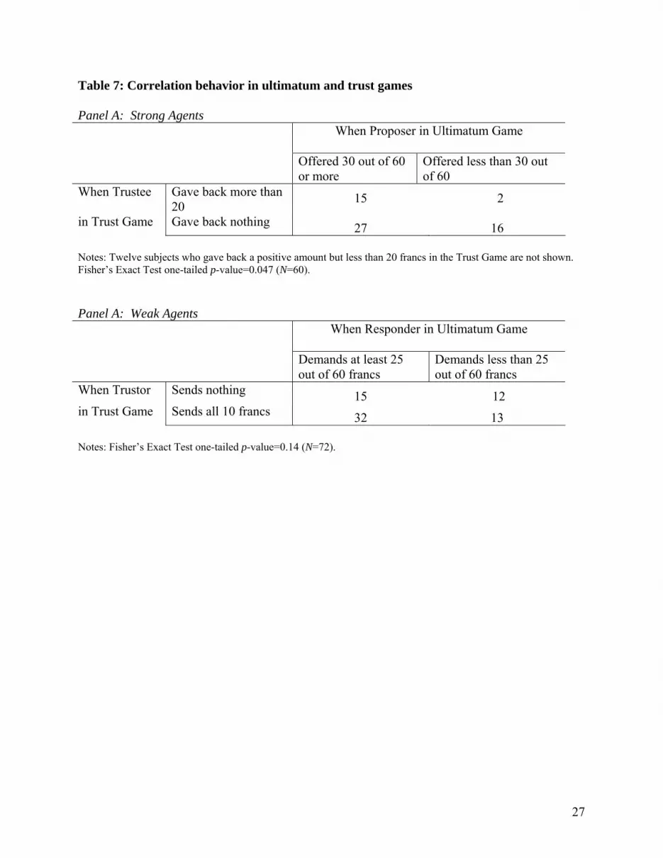
Result 3: Miscoordination occurred in about half the pairs in the Baseline and Bonus

treatments, and about one-third of the pairs in the Explicit Commitment treatment. While the

cheap talk of the Bonus treatment doubles the rate of the high effort outcome relative to the

Baseline, it does not substantially reduce miscoordination rates.

Support: Figure 2 displays the time series of miscoordination rates, and Table 2 reports

miscoordination rates in the off-diagonal (Low effort, High effort) and (High effort, Low effort)

cells, which were 51, 47 and 33 percent in the Baseline, Bonus and Explicit Commitment

treatments, respectively. The high effort outcome rate is 18 percent in the Baseline treatment and

36 percent in the Bonus treatment. Most of this increase comes from a reduction in the frequency

of the low effort outcomes and not from a reduction in the frequency of miscoordination.13

4.3 Bonus and Explicit Commitment Contract Offers

The results summarized thus far indicate that the high effort outcome was more frequent in the

Bonus and Explicit Commitment treatments where the strong agent could communicate with the

weak agent. We now analyze how the contract offers influenced behavior in the two treatments.

Result 4: In the Bonus treatment, the strong agent most frequently proposed to equally

split the earnings, but actually delivered this bonus amount only about one-quarter of the time.

Support: Figure 3 displays a bubble chart indicating the frequency of different amounts

12 For each treatment pair we run an OLS regression of session high effort rates on a treatment dummy with robust errors clustered by session (N=96). The p-values for the relevant t-tests are 0.009 for Baseline compared to Bonus, 0.011 for Bonus compared to Explicit Commitment, and 0.000 for Baseline compared to Explicit Commitment. 13 Statistical tests for overall miscoordination rates are not significant. For each pair of treatments we run a probit regression of session miscoordination rates on a treatment dummy with robust errors clustered by session (N=96). The p-values for the t-tests are 0.564 for Baseline compared to Bonus, 0.114 for Bonus compared to Explicit Commitment, and 0.108 for Baseline compared to Explicit Commitment. When we restrict to one-sided miscoordination, i.e. the weak agent exerting high effort and the strong agent exerting low effort, similar tests yield significant differences across treatments, with p-values 0.076, 0.005, 0.000, respectively.

13

of bonuses proposed and actually paid in the Bonus treatment. By far the most common bonus

proposal is to equally split earnings, 30/30, which is promised 60 percent of the time (145/240).

The actual amount paid was often less than the amount promised in this implicit contract offer,

as shown on the diagonal 45-degree line in Figure 3. Only 43 out of 174 bonuses (25 percent)

were fulfilled exactly. The strong agent only paid more than the proposed bonus in 3 out of 174

cases, and paid less than promised in 128 out of 174 promises. When failing to pay as much as

promised, the strong agent gave no bonus in 77 cases and “partially filled” the bonus with a

positive amount the other 51 times.14 The promised bonus in this environment apparently does

not activate as much “guilt aversion” as the promise does in Charness and Dufwenberg (2006).

Result 5: In the Bonus treatment, the implicit contract offer provided a one-way

communication tool to coordinate actions, with very high and low bonuses signaling the

intention to achieve the low effort outcome.

Support: High effort rates in Panel A of Table 4 were highest for intermediate bonus

amounts. The first column indicates that the weak agent exerted high effort about half the time

when the strong agent proposed a bonus of less than 50 but more than or equal to 25 of the 60

total francs available in the high effort outcome. The second column shows that in the above

situations, strong agent exerted high effort even more frequently. Both agents choose high effort

at much lower rates when the strong agent proposes no bonus or a bonus above 50 francs. In this

treatment the strong agent employed the bonus amounts to signal to the weak agent whether they

should coordinate on low effort or high effort (Figure 4). Miscoordination, which occurs when

only one agent exerts high effort, is considerably lower for very high and very low bonuses.

Average bonuses changed little over time, however, displaying only a slight increase from 26-29

francs in early periods, to 30-33 francs in later periods. This may be one reason why

miscoordination does not decline over time in the Bonus treatment (Figure 2).

Result 6: In the Explicit Commitment treatment the bonus payment provided a very

effective tool to coordinate actions. Explicit commitment led to much better coordination on high

effort than the cheap talk in the Bonus treatment.

Support: Panel B of Table 4 displays the high effort and coordination rates for various

bonus amounts. The weak agent almost never exerts high effort when the strong agent commits

14 In the bonus treatment of Fehr et al. (2007) the principals paid on average a bonus that was 64% of the amount promised when the agents gave an effort equal to or greater than requested by the principal. In our bonus treatment the strong agents paid on average a bonus that was 40% of the amount promised.

14

to pay no bonus or a bonus above 50 francs, and the strong agent exerts high effort infrequently

after indicating a bonus payment above 30 francs. When the strong agent commits to a bonus of

25 to 30 out of the 60 francs, both agents typically choose high effort and this leads to effective

coordination on the high effort outcome. This is the main source of the increased efficiency in

the Explicit Commitment treatment. The comparison of Figures 4 and 5 conveys how much

stronger of a signal the explicit contract offer is compared to the implicit contract offer.

Coordination on equilibria improved over time in the Explicit Commitment treatment, as

one can see from the trend in Figure 2. For very low or very high bonus offers, subjects typically

played the low payoff equilibrium, but for offers in the range (10, 50) subjects faced multiple

equilibria. We put forward three conjectures that could possibly explain the improvement in

coordination. One possibility is that strong agents chose more frequently offers outside the (10,

50) range. The data do not support this interpretation as the frequency of such bonus offers

actually declined over time, from 29 percent during the first 3 periods to 21 percent during the

final 3 periods. A second possibility is that the improvement in coordination is explained by

agents moving closer to the mixed strategy Nash equilibrium for offers in the range (10, 50)

range. The null hypothesis that agents play the mixed strategy equilibrium for offers in the range

(10, 50) implies a specific coordination rate for each offer level. In particular, this mixed strategy

equilibrium coordination rate is highest near the offers of 10 and 50, and is lowest for offers of

30. The data also do not support this explanation, however, because for the observed distribution

of offers the expected miscoordination rate in the mixed strategy equilibrium remains relatively

stable, around 35 to 40 percent.

The data are most consistent with a third explanation: the improvement in coordination is

due to the greater frequency of the high payoff equilibrium for offers in the range (10, 50). The

frequency of equitable offers is greater in later rounds, and such offers were more often

associated to the high payoff outcome. For example, strong agents make offers between 20 and

30 at a rate that increased from 57 percent in periods 1-3 to 72 percent in periods 7-10, and such

offers are associated with the high payoff outcome about 80 percent of the time.

4.4 Using Measured Preferences to Understand Effort Choices

Prior to facing the partnership game, subjects made three decisions without receiving any

feedback. These decisions are employed as measurements of subjects’ characteristics in terms of

15

risk attitudes, reciprocal tendencies, trusting, and trustworthy behavior, which are then applied to

understand behavior in the partnership game. Strong agents (a) made 15 binary lottery choices,

(b) made an offer to split 60 francs in an ultimatum game, and (c) decided what fraction of 60

francs to return to a first-mover in a trust game. Weak agents (a) made 15 binary lottery choices,

(b) selected a minimum offer (of 60 total francs) that would be acceptable in an ultimatum game,

and (c) made a binary decision whether to keep 10 francs or send all 10 francs (which was

increased to 50 francs) to a second-mover in a trust game.

Lottery results are reported in Figure 6. As illustrated by the dotted line, a risk neutral

agent would choose the safe option A in lotteries 1 through 7, and then switch to option B in

lottery 8. Most subjects—122 out of 144—made consistent, monotonic choices that switched

from the risky to the safe option no more than once across the 15 lotteries. Consistent with

earlier research (e.g., Holt and Laury, 2002), we find that about 6 percent of the monotonic

subjects are risk seeking (switching to the risky option before lottery 7), about 28 percent are

approximately risk neutral (switching to the risky option on lotteries 7, 8 or 9), and 66 percent

are risk averse (switching to the risky option after lottery 9). Our first result of this subsection

indicates that subjects’ measured level of risk aversion is correlated with their play in the

partnership game.15

Result 7: In the partnership game, high effort rates tend to decline with increases in

subjects’ degree of risk aversion. Moreover, in the Bonus treatment risk-seeking strong

agents propose higher bonuses but pay lower bonuses than risk neutral and risk averse agents.

Support: Table 5 reports the results of a random effect probit model of subjects’ (risky)

high effort decision in the partnership game, separately for each treatment and for the strong and

weak agent roles.16 Based on their answers to the lottery questions, participants are placed in

three categories (1) risk seeking, (2) risk neutral and moderately risk averse, and (3) strongly risk

averse. Category (2) includes subjects who switched from option A to B in lottery 8, 9, 10, or 11

and is the base case (omitted dummy variable) in the model. In three out of six columns of Table

15 For nonmonotonic subjects the risk attitude was approximated with the average among the lowest and the highest points of switch. 16 The amount that the strong agent proposes to keep, either in the cheap talk phase of the Bonus treatment or the committed amount in the Explicit Commitment treatment, obviously should influence the subjects’ propensity to choose high effort. This proposal amount is also an endogenous choice variable, so in the models of the strong agents’ high effort decision in the Bonus and Explicit Commitment treatments we use an instrumental variables approach—replacing the actual amount proposed with the predicted amount proposed, derived from the models shown in columns 1 and 4 of Table 6.

16

5 the strongly risk averse dummy coefficient is negative and significant at least at the 10 percent

level. This suggests a lower propensity to choose high effort for strongly risk averse agents.

Table 6 presents random effects estimates of models of the bonus offered by the strong

agent in the Bonus treatment (columns 1 and 2) and in the Explicit Commitment treatment

(column 4). In the Bonus treatment, risk seeking strong agents seem more prone to lying, as they

make more generous bonus proposals to weak agents when it is cheap talk but then follow-up

with less generous actual bonuses. This effect is significant at a 5 percent level.

In the ultimatum game the strong agents made proposals that were consistent with

previous research. The modal proposal was 30, half the total surplus of 60 francs. Fifty-one out

of the 72 strong agents offered 25 or 30 francs, and another 8 offered 20 of the 60 francs. The

mean proposed offer was 28.2 francs. Weak agents submitted demands in the form of minimum

acceptable offers. The modal demand, submitted by 29 of the 72 weak agents, was 30. Another

16 weak agents demanded 20 to 29 francs, and 15 demanded less than 20 francs. The mean

demand by the weak agents was 27.0 francs. A few, possibly confused subjects demanded most

of the surplus (i.e., 3 of the 72 weak agents demanded 59 or 60 francs). This partly explains the

higher rejection rate—16 out of 72 pairs (22 percent)—than is typically observed. Bahry and

Wilson (2006) provide a discussion of ultimatum rejection rates using the strategy method,

including the possible influence of confusion.

In the trust game 45 of the 72 weak agents (63 percent) chose to send the 10 francs to the

other agent. These 10 francs were converted to 50 francs, which were combined with the strong

agents’ 10 franc endowment. All 72 strong agents chose an allocation of these 60 francs, which

was carried out if their paired weak agent trusted them. A surprisingly large fraction of strong

agents, 43 out of 72 (60 percent) were not trustworthy and kept all 60 francs.17 Another 9 kept 50

francs and returned only 10. Only 6 of the 72 strong agents (8 percent) returned 30 francs, and 10

strong agents returned 20 francs. Strictly positive returns would have been earned by only 19 of

the 72 weak agents (26 percent), and the average amount returned was 7.4 francs. The high level

of trust exhibited by the weak agents is therefore surprising, and is perhaps due to inaccurate

beliefs regarding the trustworthiness of the strong agents.18

17 Note that this 60 percent untrustworthiness rate is exactly consistent with the assumed fraction of self-regarding agents used in Section 3 and borrowed from Fehr et al. (2007). 18 This lack of trustworthiness surprised us, and it differs from other binary trust games such as Eckel and Wilson (2004) who find that almost no second movers kept the entire surplus. We conjectured that this could be due to our

17

Result 8: Weak agents who trusted in the trust game were more likely to choose high

effort in the Baseline and Bonus treatments of the partnership game. Strong agents who were not

trustworthy were more likely to choose high effort in the Explicit Commitment treatment, and

were more likely to pay low actual bonuses and make bonus offers that exceed bonus amounts

actually paid in the Bonus treatment.

Support: Tables 5 and 6 provide support for Result 8. Weak agents were trustors and their

choices in the two domains were correlated, which suggest a consistent behavior across

partnership and trust games. Those subjects who sent all the money as trustors chose high effort

significantly more as weak agents (columns 2 and 4). No such correlation exists in the Explicit

Commitment treatment (column 6), suggesting that explicit contracts were perceived in a

different way from implicit bonus contracts. Strong agents that were less trustworthy (gave back

nothing in the trust game) chose high effort with greater frequency in the Explicit Commitment

treatment (column 5), which is an environment that requires less trust. By contrast, columns 2

and 3 of Table 6 show that in the Bonus treatment that requires substantial trust, untrustworthy

strong agents paid lower actual bonuses on average and failed to deliver on positive promised

bonuses.

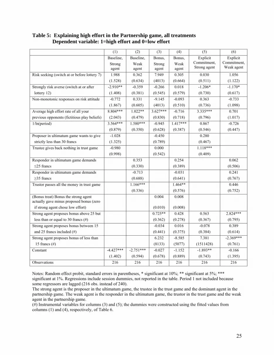
Table 7 provides additional evidence on the correlation of behavior across games. Panel

A shows that while a majority of strong agents gave back nothing in the trust game, those who

offered less than 30 francs in the ultimatum game were significantly more likely to give nothing

(Fisher’s Exact Test one-tailed p-value<0.05). The 16 (out of the total 72) strong agents who

both kept all 60 francs in the trust game and offered less than 30 francs in the ultimatum game

most clearly exhibit self-regarding preferences and apparently have more optimistic beliefs that a

substantial number of weak agents are self-regarding and would accept unequal offers in the

ultimatum game. As discussed in Section 3, this is the strong agent type that should be most

likely to exert high effort in the partnership game in the Baseline and Bonus treatments. Contrary

strategy method approach for eliciting the return decision. Results could differ between the game and the strategy method, for example, if the act of being trusted generates reciprocal feelings that are stronger than what the decision-maker feels when specifying a strategy indicating an amount returned if he is trusted. Therefore, we conducted an additional two sessions, employing 48 subjects, who only played the lottery and the trust game—but with the trust game played in the game method. Of the 17 strong agents who were trusted, 8 kept all 60 francs and only 3 split the francs 30/30. The average amount returned was greater than the strategy method trust game—11.5 compared to 7.4 francs—but this difference was not statistically significant. While the data shift in the conjectured direction, the data do not provide any strong support for our conjecture.

18

to this prediction, however, these subjects choose high effort at exactly the same rate in those

treatments (64 percent) as the subjects who do not exhibit such preferences and beliefs.19

Panel B of Table 7 shows that the pattern of weak agent behavior in the ultimatum and

trust games is not consistent with the expectation based on other-regarding preference types

hypothesized at the end of Section 3. Because inequity averse agents suffer from

disadvantageous inequality so much, unless they have very optimistic beliefs about the

trustworthiness of the strong agents they should not send the 10 francs in the trust game. These

inequity averse agents should also demand a large fraction of the 60 francs in the ultimatum

game. Contrary to this prediction, however, 32 out of the 47 weak agents who demand at least 25

out of the 60 francs in the ultimatum game trusted in the trust game (68 percent), while 13 out of

the 25 weak agents who demand less than 25 francs in the ultimatum game trusted in the trust

game (52 percent). This difference is not statistically significant, but it is not even in the

hypothesized direction since the apparently more fair-minded agents who demand more in the

ultimatum game also trust more and risk the highly inequitable (0, 60) payoff split. This suggests

a troubling inconsistency in preferences across these simple games, perhaps because this

simplified inequity aversion model is a poor approximation in the current context. For example,

the fair-minded weak agents may also have preference for efficiency and value the potential

Pareto improvement of trusting.

5. Conclusion

Other-regarding preferences have been well-documented both within and outside the laboratory

for a variety of forms of economic interactions. Empirical evidence for such preferences is now

circulating back to inform and guide positive economic theory. The goal of this paper is to

provide some laboratory evidence that explores the efficacy of implicit contracts compared to

explicit contracts in a new partnership game environment, in order to further the research agenda

“to identify the strengths and limits of the standard approach in contract theory by isolating

conditions under which the model’s contract choice predictions are met and conditions under

19 Blanco et al. (2007) also do not find substantial consistency of individual fair behavior across games. In particular, individual βi coefficients estimated from choices in a modified dictator game fail to predict behavior in the proposal role of an ultimatum game or voluntary contributions to a public good. The estimated individual βi are consistent with second-mover behavior, but not first-mover behavior, in a sequential prisoner’s dilemma game. It is conceivable that some of the inconsistency is due to subjects diversifying their risk across games, but our data do not allow us to test this conjecture.

19

which these predictions fail” (Fehr et al., 2007, p. 124). In this partnership game, other-regarding

preferences such as inequity aversion can result in large high effort rates even with implicit

contracts for certain distributions of fair-minded types. Multiple equilibria also exist in this game

with explicit contracts, including low and high effort outcomes. This underscores the importance

of new data to provide a foundation for more empirically-accurate positive theory.

Proponents and critics of using non-standard, other-regarding preferences in economic

modeling will both find some support for their cases in these data. Proponents will like the

greater high-effort rates among strong agents than weak agents, as well as the greater high effort

with implicit (cheap talk) contract offers relative to the baseline with no offers. Choices by

individual subjects are also somewhat consistent across games. For example, trustworthy strong

agents in the trust game were more likely to make generous offers in the ultimatum game, and

trusting weak agents in the trust game were more likely to exert high effort in the partnership

game. Critics can point to more and varied evidence here to support their case, most notably the

substantially greater high effort levels when moving to explicit contracts that grow over time.

Strong agents also frequently pay small or no bonuses after making generous unenforceable

bonus offers. We would conclude from these data that implicit contracts do not perform nearly as

well as explicit contracts in this partnership environment, which is an implication of standard,

self-regarding preferences.

It may be possible to improve the relative performance of implicit contracts in a variety

of ways. For example, one could make explicit agreements more costly, choose environments

such that optimal explicit incentive contracts generate zero surplus to one party, or enhance the

social connectedness of parties with rich communications. All of these variations have been

conducted by other researchers. Our experiment does not seek to explore all of the possible

factors affecting the performance of explicit and implicit contracts, but it does serve to highlight

an additional environment where explicit contracts perform better, consistent with standard

theory. We think that it is wise to explore further the boundaries of the domain where standard

theory based on the approximation of self-regarding preferences works reasonably well before

advocating a major revision of contract theory.

20

References:

Bahry, Donna and Rick Wilson (2006), “Confusion or Fairness in the Field? Rejections in the Ultimatum Game under the Strategy Method,” Journal of Economic Behavior and Organization, 60, 37-54.

Ben-Ner, Avner and Louis Putterman (2007), “Trust, Communication and Contracts: An

Experiment,” working paper, Brown University.

Blanco, Mariana, Dirk Engelmann and Hans-Theo Normann (2007). “A Within-Subject Analysis of Other-Regarding Preferences,” working paper, Royal Holloway College, Univ. of London.

Cason, Timothy and Vai-Lam Mui (2007). “Communication and Coordination in the Collective

Resistance Game,” Experimental Economics, 10, 251-267. Charness, Gary, Guillaume Frechette and John Kagel (2004). “How Robust is Laboratory Gift

Exchange?” Experimental Economics, 7, 189-205. Charness, Gary and Martin Dufwenberg (2006). “Promises and Partnership,” Econometrica, 74,

1579-1601. Eckel, Catherine and Rick Wilson (2004). “Is Trust a Risky Decision?” Journal of Economic

Behavior and Organization, 55, 447-465. Fehr, Ernst and Armin Falk (2002). “Psychological foundations of incentives,” Joseph

Schumpeter Lecture, European Economic Review, 46, 687-724. Fehr, Ernst, Alexander Klein and Klaus Schmidt (2007). “Fairness and Contract Design,”

Econometrica, 75, 121-154. Fehr, Ernst and Klaus Schmidt (1999). “A Theory of Fairness, Competition and Cooperation,”

Quarterly Journal of Economics, 114, 817-868. Fischbacher, Urs (2007). “z-Tree: Zurich Toolbox for Ready-Made Economic Experiments,”

Experimental Economics, 10, 171-178. Frey, Bruno and Margit Osterloh (eds.) (2002). Successful Management by Motivation –

Balancing Intrinsic and Extrinsic Incentives. Springer Verlag, Berlin, Heidelberg, New York.

Gächter, Simon and Ernst Fehr (2001). “Fairness in the Labour Market–A Survey of

Experimental Results,” in: Friedel Bolle and Marco Lehmann-Waffenschmidt (eds.), Surveys in Experimental Economics. Bargaining, Cooperation and Election Stock Markets. Physica Verlag.

21

Gneezy, Uri and John List (2006). “Putting Behavioral Economics to Work: Testing for Gift Exchange in Labor Markets using Field Experiments,” Econometrica, 74, 1365-1384.

Healy, Paul J., "Group Reputations, Stereotypes, and Cooperation in a Repeated Labor Market,"

American Economic Review, forthcoming Holt, Charles and Susan Laury (2002). “Risk Aversion and Incentive Effects in Lottery

Choices,” American Economic Review, 92, 1644-1655. Rigdon, Mary (2002). “Efficiency Wages in an Experimental Labor Market,” Proceedings of the

National Academy of Sciences, 99, 13348-13351. Sobel, Joel (2005). “Interdependent Preferences and Reciprocity,” Journal of Economic

Literature, 43, 392-436.

22

Table 2: Effort levels and outcomes in the Partnership game

Panel A: Baseline WEAK AGENT

High effort Low effort Totals

High effort 17.9% 36.7% 54.6%

STRONG

AGENT

Low effort 14.6% 30.8% 45.4%

Totals 32.5% 67.5% 100.0% N=480

Panel B: Bonus WEAK AGENT

High effort Low effort Totals

High effort 35.8% 36.7% 72.5%

STRONG

AGENT

Low effort 10.4% 17.1% 27.5%

Totals 46.3% 53.8% 100.0% N=480

Panel C: Explicit Commitment WEAK AGENT

High effort Low effort Totals

High effort 59.6% 28.3% 87.9%

STRONG

AGENT

Low effort 5.0% 7.1% 12.1%

Totals 64.6% 35.4% 100.0% N=480

23

Table 3: Results overview of the Partnership game

Baseline Bonus Explicit commitment

All

periods

Last 3

periods

All

periods

Last 3

periods

All

periods

Last 3

periods

Overall frequency of high effort choices 43.5% 25.0% 59.4% 47.9% 76.3% 81.3%

Frequency of mutual high effort outcome 17.9% 5.6% 35.8% 25.0% 59.6% 68.1%

Actual bonus paid by strong agents

choosing high effort (max 60 francs) 10.8 11.9 21.4

Average earnings strong agent 13.6 9.4 19.8 15.8 21.8 24.5

Average earnings weak agent 8.4 9.0 9.9 9.7 18.7 20.1

Share of earnings of strong agent 61.8% 51.1% 66.7% 62.0% 53.8% 54.9%

Efficiency (possible range from 16.7% to

100%) 36.7% 30.7% 49.5% 42.5% 67.5% 74.3%

Note: the efficiency of the low effort outcome is 33.3%

24

Table 4: Use of the contract offer as a signaling device in the Bonus and Explicit

Commitment treatments: Frequencies by level of proposed bonus

Panel A:

Bonus Treatment No. of

obs.

Weak agent

high effort

(percent)

Strong agent

high effort

(percent)

high

effort

outcome

low

effort

outcome

Miscoor-

dination

bonus ≥ 50 10 10% 20% 0.0% 70.0% 30.0%

30 < bonus < 50 33 48% 64% 30.3% 18.2% 51.5%

bonus = 30 145 53% 79% 43.4% 11.7% 44.8%

30 < bonus ≤ 25 29 52% 93% 44.8% 0.0% 55.2%

25 < bonus ≤ 10 12 17% 75% 0.0% 8.3% 91.7%

bonus < 10 11 0% 9% 0.0% 90.9% 9.1%

Panel B:

Explicit

Commitment

Treatment

Total

obs.

Weak agent

high effort

(percent)

Strong agent

high effort

(percent)

high

effort

outcome

low

effort

outcome

Miscoor-

dination

bonus ≥ 50 5 0% 20% 0.0% 80.0% 20.0%

30 < bonus < 50 4 100% 25% 25.0% 0.0% 75.0%

bonus = 30 75 99% 95% 93.3% 0.0% 6.7%

30 < bonus ≤ 25 30 80% 100% 80.0% 0.0% 20.0%

25 < bonus ≤ 10 97 54% 92% 48.5% 3.1% 48.5%

bonus < 10 29 3% 66%a 3.4% 34.5% 62.1% a This surprisingly high rate of strong agents who choose high effort after offering low bonuses is mostly due to two individual subjects (out of the 24 strong agents in this treatment). These two subjects are responsible for 80 percent of these observations.

25

Table 5: Explaining high effort in the Partnership game, all treatments Dependent variable: 1=high effort and 0=low effort (1) (2) (3) (4) (5) (6) Baseline,

Strong agent

Baseline, Weak agent

Bonus, Strong agent

Bonus, Weak agent

Explicit Commitment, Strong agent

Explicit Commitment, Weak agent

Risk seeking (switch at or before lottery 7) 1.988 0.362 7.949 0.305 0.030 1.056 (1.528) (0.634) (4013) (0.664) (0.511) (1.122) Strongly risk averse (switch at or after -2.910** -0.359 -0.266 0.018 -1.206* -1.170* lottery 12) (1.408) (0.381) (0.545) (0.579) (0.730) (0.617) Non-monotonic responses on risk attitude -0.772 0.331 -9.145 -0.093 0.363 -0.733 (1.867) (0.605) (4013) (0.510) (0.736) (1.098) Average high effort rate of all your 8.804*** 1.022** 3.627*** -0.716 3.335*** 0.701 previous opponents (fictitious play beliefs) (2.043) (0.479) (0.830) (0.718) (0.796) (1.017) 1/ln(period) 3.564*** 1.580*** -0.945 1.417*** 0.867 -0.726 (0.879) (0.350) (0.628) (0.387) (0.546) (0.447) Proposer in ultimatum game wants to give -1.028 -0.450 0.280 strictly less than 30 francs (1.325) (0.789) (0.467) Trustee gives back nothing in trust game -0.980 0.000 1.118*** (0.998) (0.542) (0.409) Responder in ultimatum game demands 0.353 0.254 0.062 ≤25 francs (0.330) (0.389) (0.506) Responder in ultimatum game demands -0.713 -0.031 0.241 ≥35 francs (0.688) (0.641) (0.767) Trustor passes all the money in trust game 1.166*** 1.464** 0.446 (0.336) (0.576) (0.752) (Bonus treat) Bonus the strong agent actually gave minus proposed bonus (zero

0.004 0.008

if strong agent chose low effort) (0.010) (0.008) Strong agent proposes bonus above 25 but 0.725** 0.428 0.563 2.824*** less than or equal to 30 francs (#) (0.362) (0.278) (0.367) (0.795) Strong agent proposes bonus between 15 -0.034 0.016 -0.078 0.389 and 25 francs included (#) (0.441) (0.375) (0.384) (0.614) Strong agent proposes bonus of less than 6.232 -8.585 7.381 -2.369*** 15 francs (#) (8133) (5077) (1511428) (0.761) Constant -4.427*** -2.751*** -0.027 -1.152 -1.893** -0.166 (1.402) (0.594) (0.678) (0.889) (0.743) (1.395) Observations 216 216 216 216 216 216 Notes: Random effect probit, standard errors in parentheses, * significant at 10%; ** significant at 5%; *** significant at 1%. Regressions include session dummies, not reported in the table. Period 1 not included because some regressors are lagged (216 obs. instead of 240). The strong agent is the proposer in the ultimatum game, the trustee in the trust game and the dominant agent in the partnership game. The weak agent is the responder in the ultimatum game, the trustor in the trust game and the weak agent in the partnership game. (#) Instrumental variables for columns (3) and (5); the dummies were constructed using the fitted values from columns (1) and (4), respectively, of Table 6.

26

Table 6: Explaining division of benefits in the partnership game, Bonus and Explicit Commitment treatments

(1) (2) (3) (4) Bonus promised by

strong agent (Bonus treatment)

Bonus actually given by strong

agent (Bonus treatment)

Bonus promised by strong agent minus

bonus actually given (Bonus treatment)

Bonus promised and given by strong agent

(Explicit Commitment

treatment) Risk seeking (switch at or before 12.441** -29.995*** 39.033*** 5.440 lottery 7) (5.859) (8.943) (9.635) (4.995) Strong risk aversion (switch at or after 0.570 -6.039* 9.059** 8.956* lottery 12) (2.167) (3.357) (3.669) (4.757) Non-monotonic responses on risk -19.980*** 24.045** -40.847*** -1.020 attitude (6.688) (10.198) (11.002) (5.201) Average high effort rate of all your -2.406 -3.549 3.758 -4.870* previous opponents (fictitious play belief)

(3.176) (2.754) (4.097) (2.950)

Proposer in ultimatum game offers -9.874*** 9.916** -13.185** 0.649 strictly less than 30 francs (3.124) (4.821) (5.240) (3.620) Proposer in ultimatum game offers -7.922** 2.348 -5.934 1.187 more than 31 francs (3.768) (5.831) (6.406) (5.558) Trustee gives back nothing in trust 2.757 -17.397*** 23.094*** -2.648 game (2.225) (3.460) (3.786) (3.572) Constant 29.423*** 31.325*** -8.359 17.210*** (4.111) (4.667) (5.881) (4.045) Observations 216 155 155 216 R-squared 0.14 0.70 0.51 0.40

Notes: Random effect regressions, standard errors in parentheses. * significant at 10%; ** significant at 5%; *** significant at 1%. Regressions include session and period dummies, not reported in the table. Period 1 not included because some regressors are lagged (216 obs. instead of 240). In columns (2) and (3) we considered only observations when the strong agent chose high effort. The strong agent is the proposer in the ultimatum game, the trustee in the trust game and the dominant agent in the partnership game.

27

Table 7: Correlation behavior in ultimatum and trust games Panel A: Strong Agents When Proposer in Ultimatum Game

Offered 30 out of 60

or more Offered less than 30 out of 60

When Trustee Gave back more than 20 15 2

in Trust Game Gave back nothing 27 16 Notes: Twelve subjects who gave back a positive amount but less than 20 francs in the Trust Game are not shown. Fisher’s Exact Test one-tailed p-value=0.047 (N=60). Panel A: Weak Agents When Responder in Ultimatum Game

Demands at least 25

out of 60 francs Demands less than 25 out of 60 francs

When Trustor Sends nothing 15 12 in Trust Game Sends all 10 francs 32 13 Notes: Fisher’s Exact Test one-tailed p-value=0.14 (N=72).

28

0%

10%

20%

30%

40%

50%

60%

70%

80%

90%

100%

1 2 3 4 5 6 7 8 9 10

Baseline

Bonus

Explicit Commitment

period

Figure 1: Frequency of the high effort outcome over time

29

0%

10%

20%

30%

40%

50%

60%

70%

80%

90%

100%

1 2 3 4 5 6 7 8 9 10

Baseline

Bonus

Explicit Commitment

period

Figure 2: Frequency of miscoordination over time

30

-10

0

10

20

30

40

50

60

0 10 20 30 40 50 60

Promised bonus

Act

ual b

onus

Figure 3: Promised and actual bonus (Bonus treatment)

Notes: Larger circles indicates more frequent outcomes. There were 240 bonus proposals. This chart displays only 174 observations, because strong agents only made an actual bonus choice when they chose high effort. Mean promised bonus: 29.6 / 60; Mean actual bonus: 11.9 /60; Frequency of promise delivered exactly or in excess: 26.4%.

31

0%

20%

40%

60%

80%

100%

50 or more more than 30,less than 50

30 less than 30 no bonus

Promised bonus

high effort outcomelow effort outcome

0%

20%

40%

60%

80%

100%

50 or more more than 30, lessthan 50

30 less than 30 no bonus

Promised bonus

high effort outcomelow effort outcome

Figure 4: Implicit contract offer as a coordination device (Bonus treatment)

Figure 5: Explicit contract offer as a coordination device (Explicit Commitment treatment)

32

0

0.1

0.2

0.3

0.4

0.5

0.6

0.7

0.8

0.9

1

lotter

y1

lotter

y2

lotter

y3

lotter

y4

lotter

y5

lotter

y6

lotter

y7

lotter

y8

lotter

y9

lotter

y10

lotter

y11

lotter

y12

lotter

y13

lotter

y14

lotter

y15

Fraction of riskychoices, obs=144

Best risk neutralchoice

Fraction of riskychoices (monotonicsubjects only),obs=122

Figure 6: Risk attitude of participants, cumulative distribution

A-1

Instructions

This is an experiment in the economics of multi-person strategic decision making. Purdue University has provided funds for this research. If you follow the instructions and make appropriate decisions, you can earn an appreciable amount of money. The currency used in the experiment is francs. Your francs will be converted to U.S. Dollars at a rate of _____ francs to one dollar. At the end of today’s session, you will be paid in private and in cash. You will also receive a $5.00 participation payment regardless of what happens in the experiment.

It is important that you remain silent and do not look at other people’s work. If you have any questions, or need assistance of any kind, please raise your hand and an experimenter will come to you. If you talk, laugh, exclaim out loud, etc., you will be asked to leave and you will not be paid. We expect and appreciate your cooperation.

This experiment is composed of four parts. Now are we are reading the instructions for part one.

Instructions– Part one

For each line in the table in the next page, please state whether you prefer option A or option B. Notice that there are a total of 15 lines in the table but just one line will be randomly selected for payment.

You ignore which line will be paid when you make your choices. Hence you should pay attention to the choice you make in every line. After you have completed all your choices a token will be randomly drawn out of a bingo cage containing tokens numbered from 1 to 15. The token number determines which line is going to be paid.

Your earnings for the selected line depends on which option you chose: If you chose option A in that line, you will receive 10 experimental francs. If you chose option B in that line, you will receive either 30 francs or 0 francs. To determine your earnings in the case you chose option B there will be second random draw. A token will be randomly drawn out of the bingo cage now containing twenty tokens numbered from 1 to 20. The token number is then compared with the numbers in the line selected (see the table). If the token number shows up in the left column you earn 30 francs. If the token number shows up in the right column you earn 0 francs. Now it is time for clarifications. Are there any questions? Participant ID: Decision no.

Option A

Option B

Please choose A or B

1 10 francs

30 francs never 0 francs if 1,2,3,4,5,6,7,8,9,10,11,12,13,14,15, 16,17,18,19,20

2 10 francs

30 francs if 1 comes out of the bingo cage 0 francs if 2,3,4,5,6,7,8,9,10,11,12,13,14,15, 16,17,18,19,20

3 10 francs

30 francs if 1 and 2 0 francs if 3,4,5,6,7,8,9,10,11,12,13,14,15, 16,17,18,19,20

4 10 francs

30 francs if 1,2 and 3 0 francs if 4,5,6,7,8,9,10,11,12,13,14,15, 16,17,18,19,20

5 10 francs

30 francs if 1,2,3,4 0 francs if 5,6,7,8,9,10,11,12,13,14,15, 16,17,18,19,20

6 10 francs

30 francs if 1,2,3,4,5 0 francs if 6,7,8,9,10,11,12,13,14,15, 16,17,18,19,20

7 10 francs

30 francs if 1,2,3,4,5,6 0 francs if 7,8,9,10,11,12,13,14,15, 16,17,18,19,20

8 10 francs

30 francs if 1,2,3,4,5,6,7 0 francs if 8,9,10,11,12,13,14,15, 16,17,18,19,20

9 10 francs

30 francs if 1,2,3,4,5,6,7,8 0 francs if 9,10,11,12,13,14,15, 16,17,18,19,20

10 10 francs

30 francs if 1,2,3,4,5,6,7,8,9 0 francs if 10,11,12,13,14,15, 16,17,18,19,20

11 10 30 francs if 1,2, 3,4,5,6,7,8,9,10 0 francs if 11,12,13,14,15, 16,17,18,19,20

A-2

francs 12 10

francs 30 francs if 1,2, 3,4,5,6,7,8,9,10,11 0 francs if 12,13,14,15, 16,17,18,19,20

13 10 francs

30 francs if 1,2, 3,4,5,6,7,8,9,10,11,12 0 francs if 13,14,15, 16,17,18,19,20

14 10 francs

30 francs if 1,2, 3,4,5,6,7,8,9,10,11,12,13

0 francs if 14,15, 16,17,18,19,20

15 10 francs

30 francs if 1,2, 3,4,5,6,7,8,9,10,11,12,13,14

0 francs if 15, 16,17,18,19,20

Questionnaire

1. If at the end of the experiment the experimenter first draws token number 2 and then draws token number 1 what are your earnings?

In case my choice for line 2 was A ______________francs

In case my choice for line 2 was B ______________francs

2. If at the end of the experiment the experimenter first draws token number 14 and then draws token number 14 again what are your earnings?

In case my choice for line 14 was A ______________francs

In case my choice for line 14 was B ______________francs

Instructions – Part two

You will participate in 12 decision making periods in the remaining 3 parts of the experiment. You will interact with another person in each of these 12 periods. You will never interact with the same person more than once, so you will interact with 12 different people.

This part of the experiment consists of one decision making period. The participants in this part of the experiment will be randomly placed into two-person groups.

Your Choices

In each group, one of you has been randomly selected to be the first mover and the other to be the second mover. You will learn which person in the group is the first-mover at the start of the period. Each person will make one decision.

There is a sum of 60 francs available. The first mover has the opportunity to decide how many francs to allocate to himself/herself and how many to the other person in his/her group (the second mover). See Figure 1 below. Up to two decimal points are allowed.

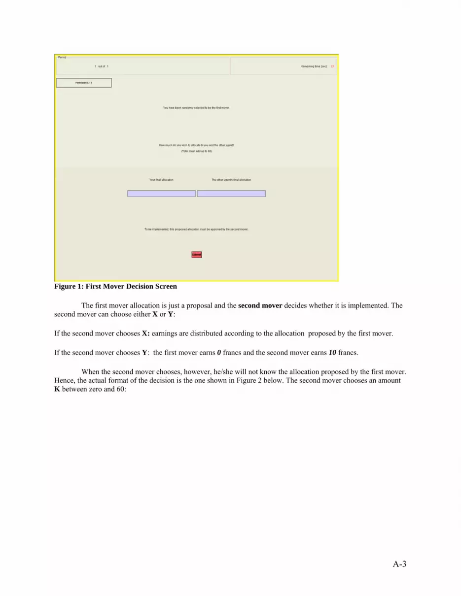
A-3

Figure 1: First Mover Decision Screen

The first mover allocation is just a proposal and the second mover decides whether it is implemented. The second mover can choose either X or Y:

If the second mover chooses X: earnings are distributed according to the allocation proposed by the first mover.

If the second mover chooses Y: the first mover earns 0 francs and the second mover earns 10 francs.

When the second mover chooses, however, he/she will not know the allocation proposed by the first mover. Hence, the actual format of the decision is the one shown in Figure 2 below. The second mover chooses an amount K between zero and 60:

A-4

Figure 2: Second Mover Decision Screen

Then, the earnings in the proposed allocation are going to be compared with K. If the proposed allocation gives to the second mover K or more francs, the choice will automatically be X. Hence, the first mover proposed allocation is implemented. If the proposed allocation gives to the second mover less than K francs, the choice will automatically be Y. Hence, the first mover earns 0 francs and the second mover earns 10 francs.

The results and earnings for this part will be communicated at the end of the experiment.

Questionnaire

3. For which of the value(s) of K listed below is a proposed allocation of (21 to the first mover and 39 to the second mover) going to be implemented? (check the appropriate boxes): 0.99 2 10 12.20 35 60

4. How much does the first mover earn if the second mover chooses Y and the proposed allocation is not implemented? _______

5. How much does the second mover earn if the second mover chooses Y and the proposed allocation is not implemented? _______

6. Which proposed allocation(s) listed below would be implemented if K is set at 49 francs? (check the appropriate boxes): (10 first mover, 50 second mover) (20 first mover, 40 second mover) (30 first mover, 30 second mover) (40 first mover, 20 second mover) (50 first mover, 10 second mover) (60 first mover, 0 second mover)

A-5

Part two results Participant ID: Your Choice: Your earnings for part two: francs Other agent’s earnings for part two: francs Part two results Participant ID: Other Agent’s Choice: Your earnings for part two: francs Other agent’s earnings for part two: francs

Instructions – Part three

This part of the experiment consists of one decision making period. The participants in this part of the experiment will be randomly placed into two-person groups. The person currently placed in your group is different from the previous one. Remember, you will never interact again with this new person in the remainder of today’s experiment.

Your Choices

In each group, one of you has been randomly selected to be the allocator. The other is the non-allocator. Each person will make one decision. First, the non-allocator chooses either X or Y. As the payoff table in Figure 1 indicates:

If the non-allocator chooses Y: there is a sum of 20 francs available; both individuals earn 10 francs.

If the non-allocator chooses X: there is a sum of 60 francs available. The person selected to be the allocator in the group will determine how many francs to allocate to himself/herself and how many to the other person in his/her group (the non-allocator). The allocator must choose numbers from zero to 60.

A-6

Figure 1: Initial Choice X or Y Decision Screen for the non-Allocator

You will learn which person in the group is the allocator at the start of the period, as shown in Figure 1 above. An example allocation screen is shown in Figure 2 below.

Figure 2: Decision Screen for the Allocator The allocator will make a decision without knowing if the non-allocator has chosen X or Y. If the non-allocator has chosen Y, the allocator decision will be ignored and her/his earnings are going to be 10 francs. If the non-allocator has chosen X, the allocator decision will determine the earnings of both persons. The results and earnings for this part will be communicated at the end of the experiment.

Questionnaire 1. The first decision is made by the allocator (circle one): TRUE FALSE 2. If the non-allocator chooses Y, does the allocator decision influence the earnings? (circle one): YES NO 3. How much does the allocator earn if the non-allocator chooses Y? _______

4. How much does the non-allocator earn if the non-allocator chooses Y? _______

Part three results Participant ID: Your Choice: Your earnings for part three: francs Other agent’s earnings for part three: francs Part three results Participant ID:

A-7

Other Agent’s Choice: Your earnings for part three: francs Other agent’s earnings for part three: francs

Instructions – Part four

This part of the experiment consists of 10 separate decision making periods. The participants in this part of the experiment will be randomly assigned to the role of either “allocator” or “non-allocator” and will keep this role for all 10 periods. Moreover, participants will be placed into two-person groups. After every period each participant will be randomly and anonymously re-matched with another participant. As explained at the start of the experiment, participants are never matched with the same participant for more than one decision period.

Your Choices

During each period, you and the other person in your group will make one, two, or three decisions. First, the allocator sends a message to the other agent regarding the allocation of a sum of 60 francs. As shown in Figure 1 below, the message is composed of the amount of his/her allocation and the other agent allocation. The two numbers must sum up to 60. The non-allocator will be waiting.

Figure 1: Decision Screen for Message to non-allocator

This message is then sent to the non-allocator and it is displayed on the non-allocator’s screen as “Message from the allocator in case both choose X: (you earn …, other earns …)” See Figure 2 below.

Second, each person has to choose either X or Y. As the payoff table in Figure 2 indicates:

A-8

If both of you choose Y this period: you both earn 10 francs.

If you choose Y and the other person chooses X: you earn 10 francs and the other person earns 0 francs.

If you choose X and the other person chooses Y: you earn 0 francs and the other person earns 10 francs.

If you both choose X: the person selected to be the allocator in the group will make a third decision. No further decision is necessary for the other person in the group.

Figure 2: Decision Screen for Initial Choice X or Y

If you are the allocator and have chosen Y, no further choice is required. If you are the allocator and have chosen X you are asked to choose how many francs to allocate to you and how many to the other person in your group. The non-allocator will be waiting. The sum of the two amounts must be 60 francs. The allocator is free to choose an allocation identical to the message sent to the non-allocator or a different one. An example allocation screen is shown in Figure 3. The allocator’s choice will be implemented when both people in the group choose X and ignored otherwise. Nobody will learn about this third choice unless both people in your group choose X.

One person in each group will be the allocator. You will learn which person in the group is the allocator at the start of the period, as shown in Figure 1. If you are an allocator in the first period, you will always remain an allocator for all 10 periods in this part of the experiment. Likewise, if you are not an allocator in this first period, you will never be an allocator in this part of the experiment.

A-9

Figure 3: Decision Screen for the Allocator

The End of the Period

After everyone has made choices for the current period you will be automatically switched to the outcome screen, as shown in Figure 3 below. This screen displays your choice(s) as well as the choice(s) of the person you are grouped with for the current decision making period. It also shows your earnings for this period.

A-10

Figure 3: Example Outcome Screen

Once the outcome screen is displayed you should record your choice and the choice of the other agent in your group on your Personal Record Sheet. Also record your current period earnings. Then click on the OK button on the bottom of your screen. Remember, at the start of each and every period of the experiment all participants are randomly re-grouped with new participants that they have not interacted with in any previous period.

After the tenth period in this part of the experiment is completed, we will randomly draw one and only one period out of these 10 periods, and you will be paid the amount that you earned for that one period only. For example, as illustrated in Figure 4, if we randomly draw period 7 as the payment period, then you and everyone in today’s experiment receive only your earnings for period 7 (for this part of the experiment), and you do not receive the earnings for the other nine periods.

A-11

Figure 4: Random Round Selection for Payment Screen

Now it is time for clarifications. Is there any question about these instructions?

Questionnaire

7. If You choose Y and the Other Agent chooses Y, then You earn , and the Other Agent earns .

8. If You choose Y and the Other Agent chooses X, then You earn , and the Other Agent earns .

9. If You choose X and the Other Agent chooses Y, then You earn , and the Other Agent earns .

10. As you are re-matched with another person after each period, there is a small probability that you will meet the same person again (circle one): TRUE FALSE

11. You will always maintain the same role (either allocator or non-allocator) for all 10 decision making periods (circle one): TRUE FALSE

12. Within a period you interact with just one other person (circle one)

TRUE FALSE

13. You will be paid the sum of the earnings from all 10 periods (circle one)

TRUE FALSE

14. The non-allocator always makes one decision each period (circle one)

TRUE FALSE

15. The allocator always makes two decisions each period (circle one)

A-12

TRUE FALSE

16. The allocation decision for the 60 francs is implemented only if both participants in the group choose X (circle one):

TRUE FALSE

17. The allocator must choose a final allocation that is identical to the message sent at the start of the period (circle one):

TRUE FALSE

Personal Record Sheet Period I am the allocator

this period (circle one)

My choice (circle one)

Other Agent’s choice (circle one)

My earnings this period

Other Agent’s earnings this period

1 Yes No X Y X Y

2 Yes No X Y X Y

3 Yes No X Y X Y

4 Yes No X Y X Y

5 Yes No X Y X Y

6 Yes No X Y X Y

7 Yes No X Y X Y

8 Yes No X Y X Y

9 Yes No X Y X Y

10 Yes No X Y X Y

Divide my earnings in selected period by conversion rate: ÷ Total earnings in for this set of periods in dollars: $ Earnings Record Sheet Part 0: Initial Participation Payment Received by Everyone, in dollars: $ 5.00 Part 1: Earnings in Experimental Francs: . Converted to dollars: $ Part 2: Earnings in Experimental Francs: . Converted to dollars: $ Part 3: Earnings in Experimental Francs: . Converted to dollars: $ Part 4: Earnings in Experimental Francs: . Converted to dollars: $ Total earnings accumulated through all parts of the experiment: $