IMPACT EVALUATION SERIES NO. 12

Extending Health Insurance to the Rural Population: An Impact Evaluation of

China’s New Cooperative Medical Scheme by

Adam Wagstaffa, Magnus Lindelowb, Gao Junc, Xu Lingc and Qian Junchengc a Development Research Group, The World Bank, Washington DC, USA

b East Asia Human Development, The World Bank, Washington DC, USA c Center for Health Statistics and Information, Ministry of Health, Beijing, China

Abstract

In 2003, China launched a heavily subsidized voluntary health insurance program for rural residents. We analyze factors affecting enrollment and combine differences-in-differences with matching methods to obtain impact estimates. We use data collected from program administrators, health facilities and households. Enrollment is lower among poor households, and higher among households with chronically sick members. The scheme has increased outpatient and inpatient utilization (by 20-30%), but has had no impact on out-of-pocket spending or on utilization among the poor. The program has increased ownership of expensive equipment among central township health centers but has had no impact on cost per case.

Corresponding author and contact details: Adam Wagstaff, World Bank, 1818 H Street NW, Washington, D.C. 20433, USA. Tel. (202) 473-0566. Fax (202)-522 1153. Email: awagstaff@worldbank.org.

Keywords: China; health insurance; cooperative medical scheme; impact evaluation.

Acknowledgements: The research reported in the paper began as a background paper for a larger World Bank study of rural health reform in China, details of which are available at http://www.worldbank.org/chinaruralhealth. The larger study was task-managed by L. Richard Meyers, and financially supported by the World Bank and the UK’s Department for International Development. We are grateful to staff from the Ministry of Health in China for support and technical advice, to Shengchao Yu and Helena Chang for their help in designing and fielding the survey and in organizing and analyzing the data, and to Bert Hofman for helpful comments on an earlier version of the paper.

World Bank Policy Research Working Paper 4150, March 2007 The Policy Research Working Paper Series disseminates the findings of work in progress to encourage the exchange of ideas about development issues. An objective of the series is to get the findings out quickly, even if the presentations are less than fully polished. The papers carry the names of the authors and should be cited accordingly. The findings, interpretations, and conclusions expressed in this paper are entirely those of the authors. They do not necessarily represent the view of the World Bank, its Executive Directors, or the countries they represent, or of the Government of China. Policy Research Working Papers are available online at http://econ.worldbank.org.

WPS4150

Pub

lic D

iscl

osur

e A

utho

rized

Pub

lic D

iscl

osur

e A

utho

rized

Pub

lic D

iscl

osur

e A

utho

rized

Pub

lic D

iscl

osur

e A

utho

rized

1

I. INTRODUCTION

Several developing countries have recently used tax revenues to subsidize health

insurance for informal sector (usually rural) workers and their families, or at least the poorer

ones among them. In Colombia, the Philippines and Vietnam, for example, the poor are enrolled

in the national social health insurance scheme at the taxpayer’s expense. The rest of the informal

sector either have the option of enrolling (in the cases of the Philippines and Vietnam) or are

required to enroll (in the case of Colombia). In all three countries, the household enrolls at its

own expense though the contribution paid by nonpoor voluntary enrollees is sometimes

subsidized (it is, for example, in the case of Vietnam). In China and Mexico, by contrast,

households not covered by formal sector programs (albeit only rural households in China) have

the option of enrolling in a separate subsidized public health insurance program. In both

countries, the contribution is to some degree linked to household income, with poor households

having their contribution paid entirely by the taxpayer, and nonpoor households either paying a

subsidized flat-rate contribution (the case in China) or an income-related contribution (the case

in Mexico).1 Thailand recently opted for a third route, which was to enroll at the taxpayer’s

expense all those not covered by the various programs for formal-sector workers.2

This paper reports the results of an impact evaluation of China’s scheme. The program,

which began in 2003 and is being rolled out on a staggered basis with all rural county-level

jurisdictions (hereafter counties3) to be covered by 2008, replaces China’s old village-based rural

health insurance program, known as the cooperative medical system or CMS.4 That scheme all

but disappeared following the collapse of the commune system in the early 1980s when China

embarked on its market-oriented economic reforms.5 As of September 2006, an estimated 406

1 To date, Mexico’s scheme has targeted the poorest decile which is not liable for contributions. 2 On Colombia see Escobar and Panoplou (2003), on Mexico see Knaul and Frenk (2005) and Scott (2006), on the Philippines see Obermann et al. (2006), on Thailand see Pannarunothai et al. (2004), and on Vietnam see Knowles et al. (2005). 3 County-level governments in China include urban districts, county-level cities, and counties. The new program is targeted at rural residents. Most (but not all) reside in counties; urban districts and county-level cities containing rural residents will also receive the program. 4 The primary stated aim of the scheme is to reduce impoverishment resulting from illness (Central Committee of CPC 2002). In 2003, piloting of the scheme began in around 300 of China’s more than 2000 rural counties in 2003 (Liu 2004; World Bank 2005). By 2005, the scheme had been expanded to over 600 counties. 5 The CMS is often argued to be at least partly responsible for China’s remarkable achievements in reducing mortality during the early years of the People’s Republic (Sidel 1993). This program was premised on mandatory contributions to the village production brigade or collective welfare fund, and ensured access to basic medical services for China’s rural population. In most part of China, CMS did not survive the de-collectivization of agriculture in the early 1980s, whereby village collective welfare funds were dismantled (Zhu et al. 1989; Liu 2004). Indeed, by 1993, less than 7 percent of the rural population was covered by the NCMS. There have been various attempts to resuscitate the CMS, including included the RAND Sichuan CMS experiment in mid-1990s (Cretin et al. 1990), the WHO 14 county study in the early 1990s (Carrin et al. 1999), the UNICEF 10- county study

2

million people were enrolled the new scheme, which was up and running in over half (1,433) of

China’s rural counties. The establishment of the new CMS or NCMS, as the new program is

known, was a response to accumulating evidence that high and rapidly rising user charges were

causing widespread poverty and deterring families—especially poor ones—from using health

facilities.6 The program—which unlike its predecessor operates at county rather than village

level, and exhibits variations in design and implementation across counties—is financed in part

through flat-rate household contributions (the poor and certain other groups have their

contributions subsidized) and in part through government subsidies, with central government

helping county governments in China’s poorer provinces with the local government contribution.

One concern with the program is that its budget is too small to make a significant dent in

households’ out-of-pocket spending. The revenue per enrolled is around only one-fifth of total

per capita rural health spending, and copayments in the scheme are high, reflecting large

deductibles, low ceilings, and high coinsurance rates. It is, in fact, possible that because the

scheme is likely to encourage people to seek care who would not otherwise have done so, and

because providers in China are paid fee-for-service through a price schedule that results in higher

margins on drugs and high-tech care than on ‘basic’ services (Liu and Mills 1999), insurance

may result in increased utilization of expensive care, and hence out-of-pocket spending may

actually increase; this appears to have happened in China’s urban scheme (Wagstaff and

Lindelow 2005). Concerns have also been expressed that the scheme may do little to increase

utilization of health services among poor households because of the high copayments. Indeed, it

has been suggested that these costs may reduce the benefits of the scheme to the poor to such a

degree that they may be less likely to enroll. Concerns have also been expressed that the scheme

may not attract the relatively good risks, and may therefore suffer from adverse selection.

This paper attempts to shed light on these and other issues, and in the process to

contribute to the more general literature on the impacts of subsidized health insurance programs

aimed at informal sector workers.7 Our focus is on the 189 counties that began implementing

NCMS in 2003. We look not only at the impacts on a large sample of households in a subset of in 1997-2000, the World Bank Health VIII project in the late 1990s, and the Harvard 2-county study in 2003 (Hsiao and et al. 2004). Many of the schemes suffer from poor administration and small risk pools. Moreover, the voluntary nature of these schemes tends to result in adverse selection. Hence, despite these efforts , coverage remained low throughout the 1990s, and by 2003, 80% of China’s rural population—some 640 million people—lacked health insurance (Ministry of Health Center for Health Statistics and Information 2004). 6 See, for example, Liu et al. (2003), Liu et al. (2004), and Yuan et al. (1998). 7 We discuss below the findings from this literature, in the context of our discussion of the findings from the present study.

3

these counties, but also at the impacts on all health facilities (township health centers and county

hospitals) in these counties. Our results are based on a comparison of changes before and after

the program’s introduction between households and facilities covered by the program and those

not covered by it. We couple this double-difference or difference-in-differences approach with

matching methods to reduce the possible biases due to the two groups having different pre-

program characteristics that may influence both changes in outcomes after the program’s

introduction and the household’s or facility’s coverage status. In our analysis of households, we

look at impacts not only for the sample as a whole but also for selected income deciles, allowing

us to explore possible differential impacts between poor households and others further up the

income distribution.

The paper is organized as follows. Section II provides a brief description of the NCMS.

Section III outlines our methods. Section IV presents our data. Section V presents the estimation

results of the model we use to estimate the propensity score for our analysis of household

impacts, and presents the results of our balancing tests. Section VI presents our estimates of the

program’s impacts, and the final section (VII) contains a summary and discussion.

II. THE NEW COOPERATIVE MEDICAL SCHEME8

NCMS differs from the old CMS in several key respects. It is a voluntary scheme.9

However, to make it fairer and financially more attractive to low-risk households, contributions

are supplemented by government subsidies. Another key difference between NCMS and the old

CMS is that the new scheme is to operate at the county level rather than at the village or

township level, thereby providing for a larger risk pool and for economies of scale in

organization and management. 10 Counties are being given considerable discretion in the design

of NCMS—the risks covered, the emphasis on inpatient and outpatient expenses, the use of

demand-side and supply-side cost-sharing, and so on. One reason for this was simply an

acknowledgement that local choice on design issues is an integral feature of China’s highly

8 This section draws on a county program survey that was done along with the household survey on which this paper is based. More details about the survey are provided in the data section below. For information about design and implementation of the NCMS, also see Mao (2005). 9 At least in part, this decision was motivated by widespread dissatisfaction in rural areas with a proliferation of fees and taxes. In order to reduce the tax and fee burden of rural residents, the government has eliminated a number of rural taxes and reduced others (Yep 2004; Lin 2005) (Tao and Liu 2005). In this context, it was seen as difficult to introduce a new mandatory charge. 10 Most rural counties have a population ranging from 200,000 to 300,000 people.

4

decentralized health system. But there was also another reason—to ensure that lessons could be

learnt from local experimentation, and that that they could be fed into the scaling-up process.

To capture better the details of the scheme at local level, we administered a detailed

program questionnaire in 17 NCMS counties.11 The program survey was complemented by a

qualitative study (Wu et al. 2006), involving focus-group discussions and semi-structured

interviews with NCMS stakeholders, including NCMS management, the local NCMS monitoring

committee, health care providers at county and township level, village leaders, village doctors,

and rural residents themselves.

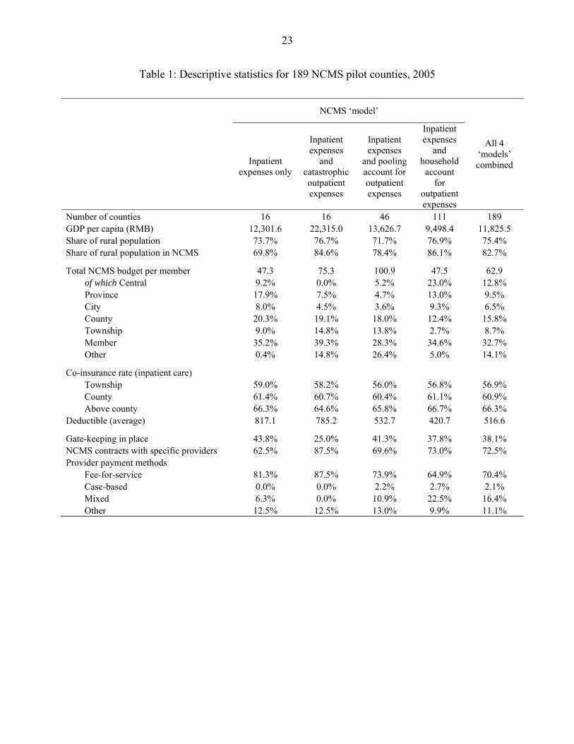
The voluntary nature of NCMS raises concerns about adverse selection. Participation

rates in pilot counties are, however, for the most part high, with an average in excess of 80

percent (see descriptive information in Table 1). In part, high levels of participation are likely to

be the result of features of the NCMS that are meant to address the problem of adverse selection,

notably the relatively generous government subsidies and the requirement that participation be at

the household level. However, the qualitative study suggests that local governments have also

exerted considerable efforts to achieve high levels of participation (Wu et al. 2006).

While central government has issued broad guidelines for how the NCMS should be

designed and implemented, provincial and county governments retain considerable discretion

over the details. One area of discretion concerns the placement of the program. NCMS pilot

counties were not randomly selected. Rather, a complex set of criteria, including local interest

and capacity, level of economic development, and the status of the delivery system were

considered. The implications of selective program placement for our identification strategy are

discussed in the methodology section below.

Local government also has some discretion over the level of financing of the program,

and the associated benefit package. Currently, the minimum requirement is a 10 RMB (per

person) beneficiary contribution from households, supplemented by a subsidy of 20 RMB from

local government (40 RMB in the case of eastern provinces), and a 20 RMB matching subsidy

from central government in the case of households living in the poorer central and western

11 A short form of the program questionnaire was also administered to all other counties (N=162) with official NCMS pilots in the 17 provinces covered by the survey. The data are not used in the present paper.

5

provinces.12 The 50 RMB minimum level of financing per beneficiary represents only around

one fifth of average per capita total health spending in rural areas.13 As can be seen from Table 1,

the total NCMS budget tends to be higher than the 50 RMB minimum (62.9 RMB on average in

a sample of 189 counties from 17 provinces), and it varies considerably with local income and

coverage mode.14

As a result of limited financing, coverage is typically shallow: many services

(particularly outpatient care) are not covered or covered only partially, deductibles are high,

ceilings are low, and coinsurance rates are high (see Table 1).15 There is, however, considerable

heterogeneity in the benefit package across counties and coverage modes. All counties cover

inpatient care. However, only a quarter of counties cover outpatient expenses on a pooling basis.

The rest do not cover them at all (10% of counties), cover only catastrophic expenses (10% of

counties), or cover them through a household account.

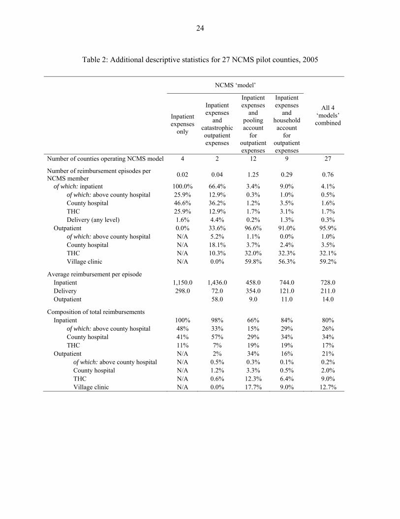
The bulk of reimbursement by NCMS is for inpatient expenses, even in counties where

outpatient expenses are covered. In the 27 counties for which data are available, the share of

reimbursements accounted for by inpatient care varies from 100% to 66%, depending on the

coverage mode (see Table 2). Most inpatient reimbursement is for care delivered at county or

provincial hospitals (75% on average), but township health centers (THCs) also account for a

substantial share of inpatient reimbursements, in particular in counties where outpatient care is

covered through household accounts or on a pooling basis.16 Most NCMS schemes have some

mechanisms to control reimbursement expenditures. For example, reimbursement rules are

typically less generous for care delivered in higher-level facilities, and most counties require 12 USD1 ≈ RMB8. 13 According to the 2004 rural household survey, average out-of-pocket expenditures for rural residents range from 47 RMB in Guizhou to nearly 587 RMB in rural areas surrounding Beijing, with a national average of 130 RMB. For the most part, this level of spending refers to a situation where households have no insurance. Insofar as health insurance makes health care more affordable at the margin, overall health expenditures are likely to increase as a result of the NCMS, reflecting both moral hazard and the ability of households to meet hitherto unmet need for health care. In addition to out-of-pocket spending, National Health Accounts estimates include spending by government and other third party payers. Estimates from 2003 suggest that total health spending in rural areas was approximately 250 RMB per capita. 14 The different approaches to defining the NCMS coverage are sometimes classified into four ‘modes’: (i) inpatient only; (ii) inpatient and catastrophic care; (iii) inpatient and outpatient pooling; and (iv) inpatient and household medical savings account. There is however considerable heterogeneity within these modes. 15 The complexity of cost-sharing arrangements causes considerable confusion among farmers about what can and cannot be reimbursed, and how much will be reimbursed. 16 Village health posts comprise the first level of contact in the health system operating in rural areas. At the second tier, Township Health Centers (THC) serve as the first referral level. They have an average of 15-20 beds and provide both preventive, outpatient, and basic inpatient care. At the third tier, there are nearly 6,000 country hospitals—usually the last point of referral for the rural population—with an average of 300 beds. In contrast to the rural health system, which is the responsibility of county or township governments, the approximately 11,000 city hospitals are the responsibility of provincial or prefectual government. Complex cases from rural areas may be referred to these higher levels.

6

members to use only certain approved facilities. However, few counties use one of the most

obvious forms of cost control, namely a provider payment method other than fee-for-service

(Table 1).

In parallel with the introduction of the NCMS, the government has also set up a medical

assistance (MA) scheme aimed at assisting poor and certain other types of households, as well as

near-poor households facing high health care expenses.17 Recent years have also seen efforts to

improve service delivery. Since the economic reforms of the early 1980s, financing and

regulatory arrangements have created perverse provider incentives, and resulted in problems of

inefficiency, low quality, and unnecessary care (World Bank 2004; Blumenthal and Hsiao 2005).

Despite reform efforts, many of these problems remain pervasive.

III. METHODS

We estimate the impacts of NCMS on individual, household and health facility outcomes

by combining differences-in-differences or double-differences (DD) with matching methods, an

approach that is becoming increasingly common in the impact evaluation literature (cf. e.g.

Chen, Mu and Ravallion 2006; Wagstaff and Yu 2006; Ravallion 2007).18 Health facilities are

classified as ‘treated’ if they are located in NCMS counties, and as ‘untreated’ otherwise.

Households are classified as ‘treated’ if they are NCMS members, and as ‘untreated’ if they are

not. In our main results, the latter are households living in NCMS counties who chose not to join,

but we also explore a second definition of ‘untreated’ households, namely those living in

counties where NCMS has not yet been introduced.

We compare average changes in outcomes before and after the introduction of NCMS

between treated and untreated units (i.e. facilities or households), using matching to control for

(initial) heterogeneity in terms of observable variables. A simple comparison between ‘treated’

and ‘untreated’ units after the program’s implementation (i.e. a single difference) would give a

biased estimate of the program’s impact if factors influencing enrollment in the program or

placement of the program were also correlated with post-treatment outcomes. Matching would 17 MA covers households in China’s wubao, tekun and dibao anti-poverty programs, as well as the near-poor who suffer from chronic illness. It is financed from multiple sources, including government budget, donations, and lottery income. Where NCMS is already up and running, it enrolls MA beneficiaries in NCMS. 18 For excellent reviews of the recent impact evaluation literature, see Imbens (2004), Blundell et al. (2005) and Ravallion (2007). For a useful practical guide to PSM, see Caliendo and Kopeinig (2005).

7

remove any bias caused by selection on observable variables, but would leave the possibility of

bias due to selection on unobservable variables. It is plausible, for example, that people enrolling

in NCMS have unobserved characteristics that predispose them to higher out-of-pocket

spending—i.e. the scheme suffers from adverse selection. A single difference between the

treated and untreated after the program’s introduction—even after matching—would give an

upward biased estimate of the program’s impact, and may even show the program increasing

out-of-pocket spending. This turned out to be the case with the dataset used in this paper. By

combining matching with double differencing we can remove any bias due to selection on time-

invariant unobservables. This is analogous in a regression setting to estimating a fixed-effects

model on panel data collected before and after the program’s implementation, while single

differencing with matching is analogous to estimating a regression on data collected after the

program’s implementation. The identification assumptions in the regression and matching

approaches are the same, but the matching method has the attraction of not requiring the

specification of a model (let alone a linear model) for the outcome; all that is required as far a

model is concerned is the estimation of a probit (or similar) to obtain the propensity scores (cf.

e.g. Jalan and Ravallion 2003; Ravallion 2007).

It is conceivable that NCMS may have spillover effects on nonmembers. If this is the

case, we need to be clear about what is being measured when comparisons are made between

members in the scheme and the two comparison groups (Janssens 2005). Suppose that facilities

get upgraded as a result of NCMS or in anticipation of NCMS’s rollout. These changes may

improve the quality of care or other attributes of service use, such as convenience. Nonmembers

as well as members may benefit, and increase their utilization. Or suppose that following

NCMS’s introduction, providers start following guidelines and protocols on the use of drugs and

diagnostic tests, and that they abide by them for nonmembers, as well as members. Even

nonmembers would benefit in terms of lower out-of-pocket spending and better quality care, and

may be encouraged to use facilities more. Then comparing members and suitably matched non-

members in NCMS counties would understate the total benefits of NCMS; it would provide a

measure of the net benefits accruing to NCMS members—the extra benefits accruing to people

in NCMS counties who opted to join NCMS. Or it may be the case that non-members are

adversely affected by NCMS. For example, providers may respond to NCMS cost-containment

measures by inducing more demand for their services among nonmembers. So, while NCMS

8

may reduce out-of-pocket spending among members, it may increase it among nonmembers—a

negative spillover effect. Comparing participants with suitably matched people in counties

without a NCMS will reveal the gross effects of NCMS—the benefits accruing to members, plus

(or minus) any spillover effects accruing to nonmembers. If the member-nonmember comparison

produces a larger impact than the comparison between members are matched people in non-

NCMS counties, the implication is that there are positive spillovers. In the event, because of the

dissimilarity between our five control counties and our ten ‘treatment’ counties, we are unable to

shed any light on the issue of spillovers.

The matching method we use in the case of households is propensity score matching

(PSM). The propensity score measures the closeness (in terms of a vector of initial conditions) of

‘treated’ and ‘untreated’ households, the score being the predicted probability of a household

participating in NCMS. A treated household’s change in outcome is compared with a

counterfactual change in outcome, formed as a weighted average of the changes in outcomes of

untreated households, where the weights reflect the propensity scores, the exact weighting

scheme depending on the variant of PSM used (discussed below). The differences in changes (or

differences) are then averaged to get the average treatment effect (on the treated). The probit

used to obtain the propensity scores is inevitably estimated only on the subsample of households

living in counties where NCMS is operating. When the comparison group is households in non-

pilot counties, the propensity scores for those individuals are predicted from the model estimated

on the sample from the pilot counties; this, as will be seen below, creates insuperable problems

in this particular evaluation.

We use all households units in the control group to construct the counterfactual outcome

for treated households, using kernel matching. This can be thought of as a weighted regression of

the outcome on the treatment indicator variable, the kernel weights being a decreasing function

of the absolute difference in propensity score between the treated and untreated unit (Smith and

Todd 2005).19 We check the sensitivity of our results to the choice of estimator by also reporting

results where treated and untreated cases are matched via weights based directly on the

propensity score. This estimator can also be implemented as a weighted regression of the

outcome on the treatment indicator, where the weight is one for a treated unit, and P/(1-P) for the

untreated unit, P being the (estimated) propensity score (cf. Imbens 2004). The regression 19 We used a normal (Gaussian) kernel and a bandwidth of 0.06.

9

implementation reduces the computational burden, substantially in the case where there are many

outcome indicators, as in the present application.20 A further attraction is that it facilitates

estimates of differences in impact across subsamples. In the present context, given the concern

about the health spending and under-utilization of health care among China’s poorest

households, an obvious dimension along which to explore differential impact is income. By

regressing the outcome on the treatment indicator, the income category dummies, and

interactions between the two, weighting the regression by the kernel or propensity score weights,

one can conveniently obtain estimates of the impacts for the different income groups.21 The

regression using propensity score weights leads directly to robust standard errors. In the case of

kernel matching, we report obtain regression-based standard errors as well as standard errors

obtained through bootstrapping with 100 replications.22

All facilities in a given county are ‘treated or ‘untreated’. In this case, we still want to

match on initial conditions, some at county level, but some too at facility level. The concern is

that without matching, the initial conditions of the facilities and the county in which they are

located might have influenced both the change in outcomes and the likelihood of the county

being chosen as one of the initial NCMS counties. PSM could be used in such a setting. We

could, for example, as in Wagstaff and Yu (2006), estimate a probit accounting for the selection

of NCMS counties, either with county-level data or a mixture of county- and facility-level data,

and obtain a propensity score for different facilities (a county average would need to be applied

to all facilities in a given county in the case where county- and facility-level data are used). In

the event, partly because we have relatively few variables on which we want to match, we

decided to match directly on our limited set of variables, using the Mahalanobis metric to trade

off closeness on one dimension against closeness on another. To ensure comparability, ‘treated’

(i.e. NCMS) facilities are matched insofar as is possible with facilities in the same province. We

used nearest-neighbor matching, with five neighbors. With nearest-neighbor matching, a caliper

20 The regression routine in Stata is much faster than psmatch2 or other matching routines. The kernel weights need be estimated just for one outcome (which can be done using psmatch2), and then used in regressions for the other outcomes. 21 This method also provides a simple way to obtain impacts for different income groups using the DD without matching. With or without matching (i.e. weighting), the impact for a particular income group is the sum of the coefficient on the NCMS treatment indicator plus the coefficient on the interaction between the treatment dummy and the income group dummy. 22 The reservations that have been expressed about bootstrapping standard errors in matching do not apply to the kernel method, because it does not run into the discontinuities that arise in nearest-neighbor matching (see e.g. Imbens 2004).

10

has to be selected: we opted for a caliper of 0.5, and found the results insensitive to the choice of

caliper.23 We compute standard errors for the facility impacts using bootstrapping.

It is standard practice in applications of PSM to limit comparisons to a subset of cases to

ensure comparability. One approach is to focus on units lying on the common support of

propensity scores. Our focus is on the effect of NCMS on the ‘treated’—i.e. the average

treatment effect on the treated, or ATT. Given this, imposing the common support would entail

excluding treated households with propensity scores that are larger than the maximum propensity

score observed in the untreated group.24 In this application, this would result in dropping

relatively few treated households. A less ad hoc approach, and the one adopted in this paper, is

that suggested by Crump et al. (2006): the sample is selected so as to minimize the variance of

the estimated average treatment effects.

IV. DATA

The analysis is based on panel data from 12 provinces.25 The starting point for

constructing the panel was the 2003 round of the National Health Service Survey (NHSS),

administered by the Center for Health Statistics and Information (CHSI) of the Ministry of

Health (MOH).26 The NHSS collects data on, among other things, general household and

individual characteristics, health status, use of health services, and health related expenditures.

The 2003 NHSS covered approximately 54,000 households in 900 villages across all 31

province-level units, with counties, townships, villages, and households selected using a used a

multi-stage stratified random sampling strategy.

A follow-up survey, in which households in the 2003 NHSS were re-interviewed, was

implemented by the CHSI in the fall of 2005. This survey covered 10 counties that had begun

piloting the NCMS in the intervening period since the 2003 survey was fielded and 5 that had not

23 Results are available on request. 24 If we also wanted to estimate the average effect of treatment on the untreated and the overall average treatment effect, the common support would also exclude untreated cases with a propensity score smaller than the smallest propensity score in the treated group. 25 Details on survey design and implementation, as well as extensive descriptive analysis, can be found in Center for Health Statistics and Information (2005; 2006). The former is available upon request from the authors. 26 The first NHSS was implemented in 1993, and it has since been implemented every five years.

11

begun piloting.27 The 10 program counties were the only ones out of the 90 counties in the 2003

sample that were running official NCMS pilots.28 Efforts were made to ensure that the 5 non-

NCMS counties were similar in relevant respects to the NCMS counties. This was done by

estimating the probability of a county being selected as an NCMS pilot county, and finding

(among the 2003 NHHS counties) non-pilot counties that had similar probabilities (i.e.

propensity scores) to the pilot counties.29 The resultant sample includes counties from all regions

and all four NCMS ‘coverage modes’. However, given the opportunistic sample design, sample

descriptives cannot be seen as representative for China as a whole, or for any specific province

or region.

The follow-up survey successfully re-interviewed approximately 94 percent of all

households, and around 87 percent of individuals from the 2003 sample.30 There was no

significant difference in the gender distributions of those originally interviewed and those not

reinterviewed, but there was a difference in the age distributions, with missing individuals being

more likely among the 15-34 age group. Due to missing values and other problems in the data,

around 9 percent of observations were dropped in the analysis. The result is a sample of 8,476

households and 28,696 individuals in the 15 counties (5,641 households and 18,337 individuals

in the 10 NCMS counties).

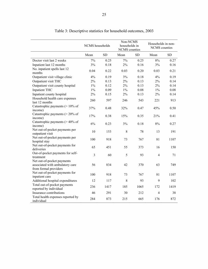
Table 3 reports baseline descriptive statistics for the outcomes studied for NCMS

households, non-NCMS households living in the ten NCMS pilot counties, and households in

living in the five non-NCMS counties. The utilization of health services is similar among all

three groups, with a slight tendency towards higher rates among the NCMS households. Health

spending is captured in the survey both through the household expenditure module, where

households are asked how much they spent in the previous 12 months on health care, and in the

specific utilization modules, where each individual in the household is asked, for each category 27 The survey also covered an additional 17 counties without baseline data. This was done to generate more extensive and representative descriptive data. The cross-section data are not used in this paper, because as indicated earlier, estimates based on cross-section data are likely to be biased in this context because of the influence of unobservables in the enrolment process. 28 The sample include counties from all the different coverage modes (2 inpatient only, 2 inpatient and catastrophic care, 2 inpatient and outpatient pooling, and 4 inpatient and household accounts), and from all regions (5 east, 2 center, and 3 west). 29 The probit was estimated on 2070 counties, using data from the National Bureau of Statistics county database. The variables that were significantly related to whether or not a county was selected as an NCMS pilot were: GDP per capita, the rural share of the population, and investment in fixed assets, all of which increased the likelihood of the county being selected, and the fraction of the population in middle school, which was negatively associated with being a pilot county. Variables included but which had an insignificant coefficient included: electricity use, telephone lines, fiscal revenues, government expenditures, industrial output, primary enrollment, beds in government hospitals, welfare institutions, and beds in welfare institutions. 30 Quality control measures in data collection and entry included extensive enumerator training, detailed review and control of five percent of sample in the field by supervisors, and double entry of data.

12

of service, how much they spent over the period specified in the utilization question, and how

much they were or would be reimbursed by an insurer (including NCMS) or a government

welfare program. The household health expense and catastrophic spending variables in Table 3

are derived from the household expenditure module (all are adjusted for household size), and the

remaining health spending questions are derived from the individual utilization modules. The

insurance contribution variable relates to all insurers. The NCMS households incurred somewhat

higher health expenses in the baseline, in part because of higher spending per inpatient stay.

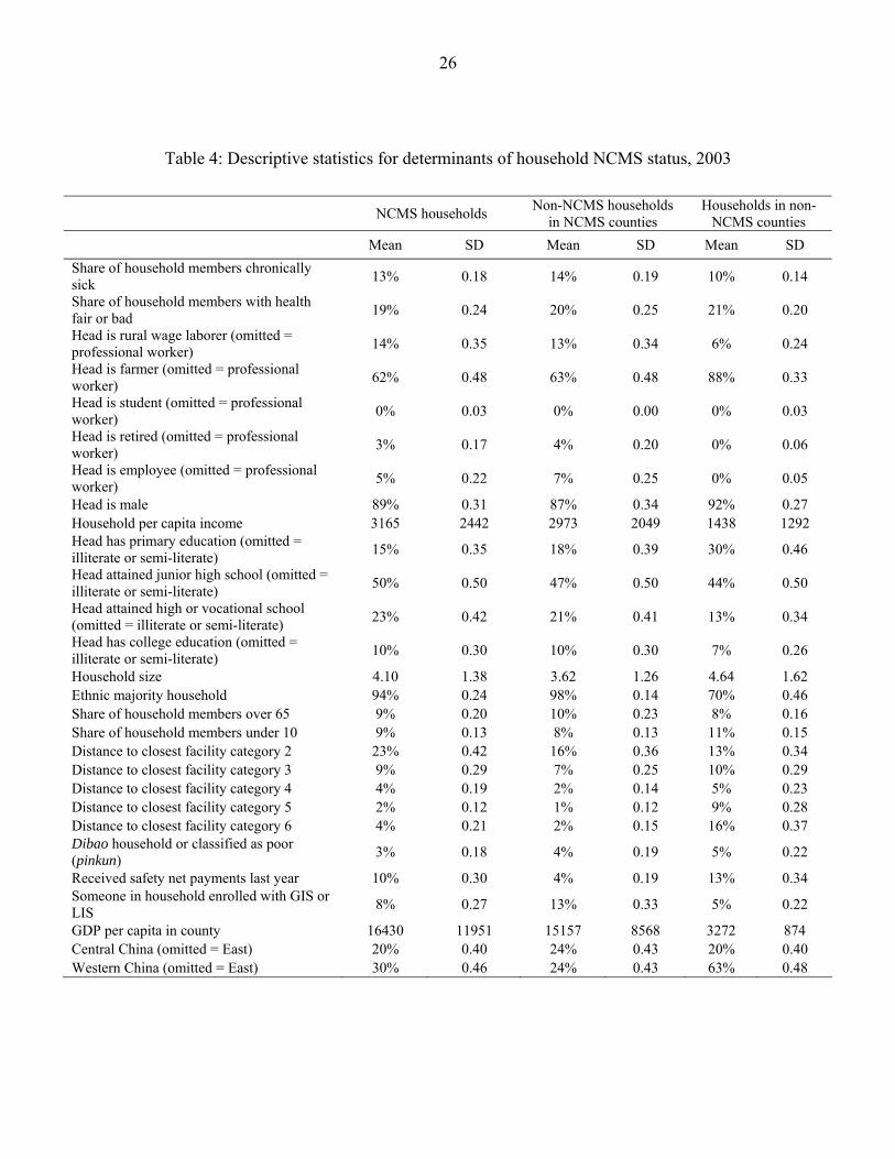
Table 4 reports the descriptive statistics of variables that might plausibly affect

enrollment in NCMS. In general, NCMS households and households not enrolled in NCMS but

living in NCMS counties are fairly similar to one another. Both tend, however, to be quite

different from households living in the five non-NCMS counties. The latter are more likely to be

(peasant) farmers, tend to have a lower per capita household income, are more likely to belong to

one of China’s ethnic minorities, tend to live further from a health facility, are more likely to be

classified as poor or to be covered by China’s new rural safety net program known as dibao,

more likely to have received payments from dibao or another welfare program in the previous 12

months, and to be living in one of China’s (poorer) western provinces.

Finally, the paper draws on provider data from a MOH administrative database that

contains annually updated data on all health care providers in China, the data being supplied by

the providers themselves according to a standardized set of forms. From the database we use data

on all THCs and all county hospitals in all 15 provinces and 2 municipalities that piloted NCMS

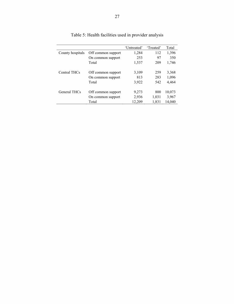
in the first wave. We therefore have ‘treated’ facilities in around 200 counties, and ‘untreated’

facilities in around 1,500. Separate analyses are reported for county hospitals, central THCs and

general THCs. The total number of county hospitals, central and general THCs included in the

analysis is 1,746, 4,464 and 14,040 respectively (Table 5). Of these, 209, 542 and 1,831

respectively were located in NCMS counties. Roughly half of these were discarded because they

were too different from facilities in non-NCMS counties to be considered close matches (i.e. they

were off the ‘common support’). And only around 20% of potential control facilities were, in the

event, used as controls, the others being too different (i.e. off the common support).31 The dataset

includes a variety of outcomes of interest, including: total revenues, as well as the share coming

31 Some facilities do not have data on all the outcomes, and the numbers on and off the common support vary somewhat from one indicator to the next.

13

from subsidies; total expenditures, including the share going on salaries, and expenditure per

case; staff numbers, including the fraction of which are retirees; the number of items of

equipment costing in excess of 10,000 RMB; inpatient discharges; the bed occupancy rate;

length of stay; and the number of outpatient visits.

V. PROPENSITY SCORE ESTIMATION AND BALANCING

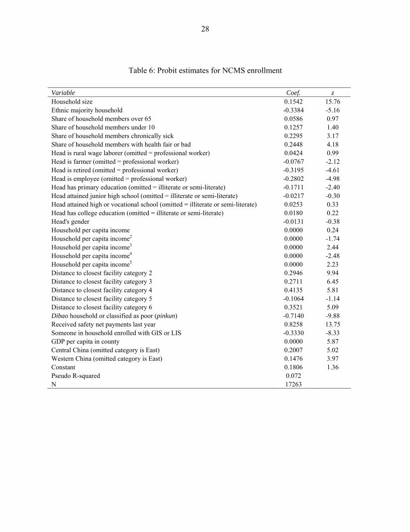
Table 6 reports the results for the probit model used to obtain the propensity scores. Since

the NCMS decision is a household one, the variables are all defined at the household level, or

higher. To weight the data by household size, the model is estimated on individual data, the data

coming from the 2003 survey.

The results suggest that larger households are more likely to enroll in NCMS, and that

ethnic minority households are more likely to enroll. The age structure of the household makes

no difference to its probability of enrolling. By contrast, its health status does. Households with

larger shares of chronically sick members and those with larger shares of members reporting

their health as bad or fair (as compared to good or excellent) are more likely to enroll. NCMS

seems, therefore to be suffering from adverse selection on observables. Ceteris paribus,

households whose head is a rural wage laborer are no more likely to enroll than those whose

head is a professional worker, while households whose head is a farmer, retiree or employee are

less likely to enroll. Households whose head completed primary school only (as compared to no

schooling) are less likely to enroll, but otherwise educational attainment does not predict

enrollment, holding other variables constant. The gender of the household head makes no

difference to the likelihood of it enrolling. Its income, by contrast, does. The polynomial points

to a highly nonlinear relationship between enrollment probability and income, with dips at the

bottom and middle of the income distribution. Households living far away from facilities are less

likely to enroll, but increasing distance reduces the probability only up to a point. A household

officially designated as ‘poor’ (pinkun) is less likely to enroll, holding other factors—including

income. Receipt of a safety net payment in the previous year, by contrast, increases the

likelihood of enrollment. Households with one or more members in the urban schemes (GIS or

LIS) are less likely ceteris paribus to enroll in NCMS. Households living in richer counties are

14

more likely to enroll, as are households living in central and western China (relative to

households living in eastern China).

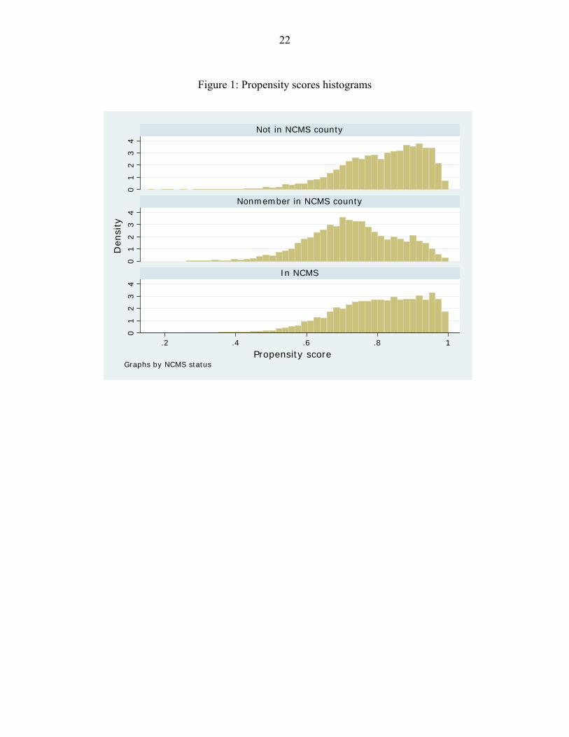
Figure 1 shows the histogram for the propensity scores for the three categories: NCMS

households, non-enrolled households living in NCMS counties, and households living in non-

NCMS counties. Unsurprisingly, there is more density to the right of the propensity score

distribution (the distribution is more skewed to the left) in the case of NCMS households than in

the case of non-enrolled households living in NCMS counties. However, the region of common

support is ample. By contrast, there is more (left) skewness in the propensity score distribution

for households living in non-NCMS counties than in the distribution for NCMS households, and

the mean propensity score is higher too (0.816 compared to 0.814). Households living in the

sampled non-NCMS counties are clearly different from those living in the sampled NCMS

counties. Using the criterion proposed by Crump et al. (2006), the optimal propensity score

cutoff points in the case where non-enrolled households are the control group turned out to be

0.0893 and 0.9107. This interval lies well within the region of common support, and we end up

dropping 2,276 treated and 272 untreated individuals. In the case where households living in

non-NCMS counties are the control group, the range turned out to be 0.0815-0.9185, and we

ended up dropping 2,099 treated and 2,041 untreated individuals.

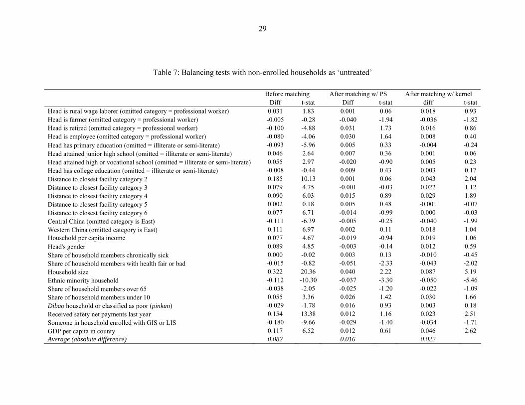
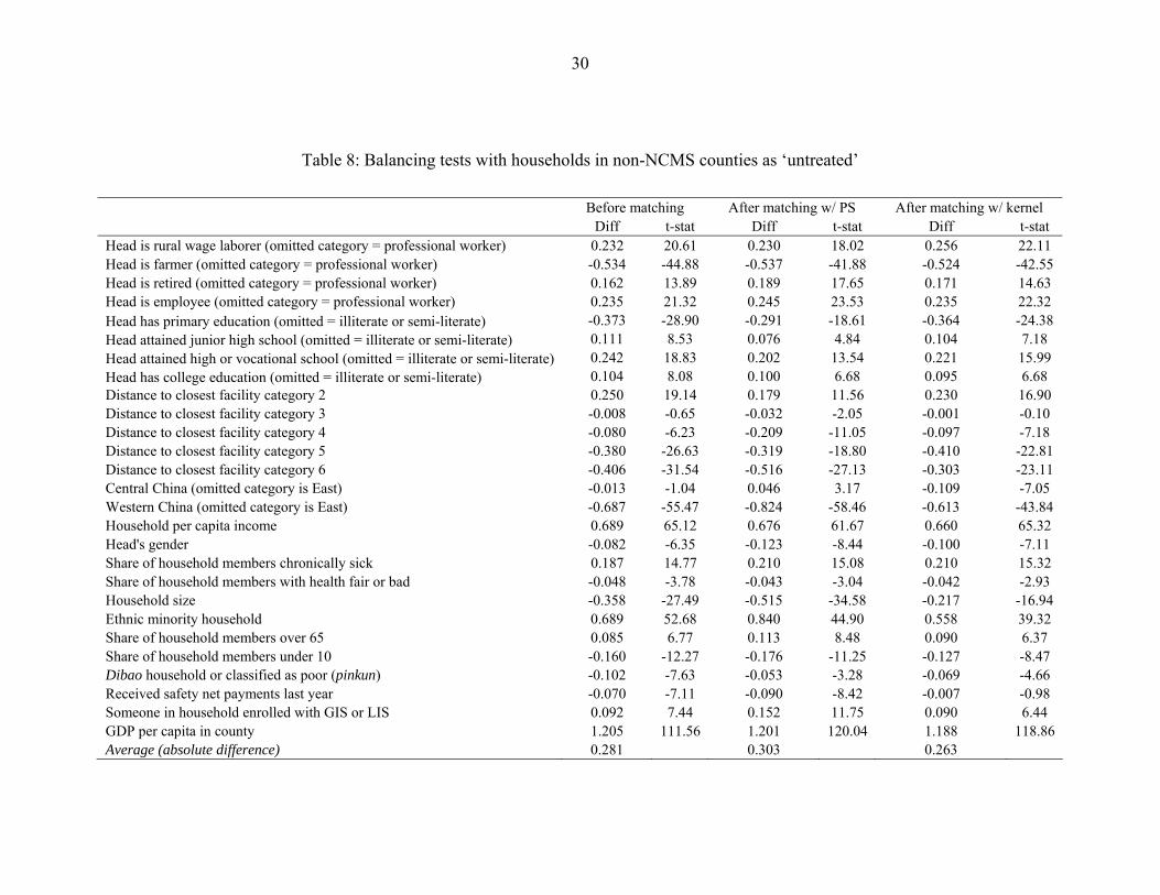
Table 7 and Table 8, which report the results of balancing tests, make the above-noted

differences even clearer. In Table 7, the control group are non-enrolled households, and in Table

8 they are households in counties where NCMS has yet to be implemented. In both tables, the

samples are the trimmed samples, and the variables used in the probit model have been

standardized with reference to the sample means and standard deviations. The idea is that once

the untreated observations have been appropriately weighted, and the sample has been trimmed

suitably, there should be no association between treatment status and each standardized

covariate. The first column in each table shows the standardized differences before matching.

The average absolute standardized difference is considerably larger when the control group

comprises households in non-NCMS counties. The second column shows the differences on the

common support after weighting using the propensity score, and the third the standardized

differences using the kernel-based weights, again on the region of common support. In Table 7,

the trimming of the sample and both methods of weighting result in a much greater degree of

balance in the covariates. In Table 8, by contrast, there is little—if any—balancing achieved

15

through trimming and weighting. The implication is that it is not just that the households in the

sampled non-NCMS counties are quite different in terms of the probit model’s covariates from

the enrolled households, but that the probit estimated on NCMS county households is a poor

basis on which to match NCMS households with households living in non-NCMS counties.

Because of the lack of balancing achieved when the controls are households in non-NCMS

counties, the results below are exclusively for the comparison between enrolled households and

non-enrolled households living in NCMS counties.

VI. IMPACT ESTIMATES

Table 9 and Table 10 report the household-based estimates of NCMS impacts on health

service utilization and household health spending. Table 11 reports selected impacts by income

decile. Included in Table 9 and Table 10 are the changes before and after the introduction of

NCMS for NCMS counties as a whole, for NCMS and non-NCMS households separately, and

the difference in these latter two changes (i.e. the basic difference-in-difference estimator

without any adjustment for differences in initial conditions). Also included are the two sets of

matching estimates, the first weighting the observations of non-enrolled households by their

propensity score, and the second weighting by the kernel weights. The t-statistics are based on

bootstrapped standard errors in the case of the kernel weighted results with 100 replications. The

decile-specific ATT estimates in Table 11 were obtained using kernel weighting. Table 12

reports the impacts of NCMS on health facilities—separately for general THCs, central THCs,

and county hospitals. Matching variables included 2003 (i.e. pre-NCMS) values of ownership

(government, public, or other), ‘sponsor’ (small city county, rural county, urban township, rural

township), actual number of beds, total number of staff, space owned by the facility, GDP per

capita of the county, government health spending of the county (more precisely ‘total operating

expenses on public health’), and province (including this encourages but does not force matching

by province). The ATT estimates are reported as percentage changes on pre-NCMS averages to

facilitate comparisons across outcome measures and facility types. The t-statistics in Table 12 are

based on bootstrapped standard errors with 50 replications.32

32 It could be argued that confidence intervals are meaningless, as the dataset is a census of facilities rather than a sample. However, through the matching process, not all ‘treated’ or ‘untreated’ facilities are used, which may be argued to provide a rationale for computing standard errors.

16

The household estimates in Table 9 suggest NCMS had a statistically significant positive

impact on outpatient visits (a 23% increase), but only at THC level. The facility results in Table

12 are consistent with this, but imply that significant effects on outpatient visits occurred only

among central THCs, not among general THCs. Both household and facility results also point to

NCMS increasing inpatient spells (a 27% increase according to the household data). However,

while the household results hint that the extra spells took place in county hospitals, the facility

results suggest that they occurred in THCs, especially in general THCs. This may be because the

household data are from a sample, and the facility data capture all facilities in provinces where

NCMS was being piloted at this stage. The results in Table 12 suggest that the extra inpatient

spells at THC level were achieved by increases in the rate of bed occupancy rather than by

shorter lengths of stay.

The decile-specific results in Table 11 point to some interesting differential impacts of

NCMS on utilization across income groups. In the poorest decile, no impacts on outpatient

utilization are evident at all, the impacts being evident only in deciles 2-10. There are no impacts

on inpatient utilization evident either for the poorest decile; statistically significant positive

impacts are to be found only in deciles 3-10. There is, in fact, a hint that NCMS may have had

some dampening effect on inpatient utilization among the second decile, but the evidence is not

strong. Thus NCMS does not seem to have increase utilization among the poorest 10% of

China’s rural population.

The facility results in Table 12 point to NCMS having a significant positive impact on the

revenues of THCs but not of county hospitals. In the case of central THCs, the revenue increase

is at least in part due to extra subsidies, while in the case of general THCs, the increased revenue

is entirely extra ‘business’ revenue. NCMS appears to have increased expenditures by less than

revenues in the case of central THCs, but by more than revenues in the case of general THCs.

NCMS does not appear to have significantly increased (or reduced) the cost per case (unadjusted

for casemix). The increased facility revenues and business income do not necessarily imply, of

course, that households’ out-of-pocket payments net of reimbursement have increased. Indeed,

the rise in business revenue is consistent with a fall in out-of-pocket payments net of

reimbursement. In the event, however, it appears that NCMS has had no statistically significant

effect either way on average out-of-pocket spending by households, overall or on any specific

type of care (Table 10). Furthermore, there is no evidence that NCMS has reduced the outlays

17

per contact, for either outpatient or inpatient care; indeed, there is a hint that it may have

increased the cost per inpatient episode. The impact on average household out-of-pocket

spending tells us nothing about the impact on the incidence of large payments. In the event,

NCMS appears to have increased the incidence of catastrophic household out-of-pocket

payments, at least where the catastrophic threshold is 20% or less of income. This is consistent

with the increase the scheme has had on utilization and with recent research pointing to a

positive impact of China’s urban insurance scheme on catastrophic health spending (Wagstaff

and Lindelow 2005).

Table 11 points to some interesting differences across income groups in the impact of

NCMS on household out-of-pocket spending. The program seems to have increased average out-

of-pocket spending among the poorest decile, but to have reduced the incidence of catastrophic

spending among this group. It appears, in other words, to have compressed the distribution and

shifted it rightwards. By contrast, NCMS appears to have increased the incidence of catastrophic

spending among deciles 3-10, leaving average spending unaffected.

VII. DISCUSSION AND CONCLUSIONS

This paper has reported findings on the impact of a new health insurance scheme for rural

areas in China, focusing on both the demand and the supply sides. Impacts are estimated by

combining differences-in-differences and matching methods. Short of a fully randomized

evaluation, this approach is arguably the most effective way of dealing with the potential

problem of biases arising from observed and unobserved heterogeneity in estimating the impact

of health insurance.

The results suggest that, despite its relatively short life and limited financing, the NCMS

has had substantial impacts. It has resulted in an increase of over 20% in both outpatient visits

and inpatient episodes. In the case of outpatient care, the household data suggest that most of the

increase has been at THC level, while the increase in inpatient episodes is mainly accounted for

by county hospitals. Given high coinsurance rates, it is perhaps not surprising that there has been

no significant increase in utilization among the poorest quintile. Narrow coverage and high co-

insurance rates also go some ways towards explaining why we find no evidence of the NCMS

reducing either out-of-pocket spending or the incidence of catastrophic expenditures. The results

18

from the supply-side data are broadly consistent with those of the household data, and also show

that the NCMS has had significant impacts on bed-occupancy, staffing, and capital investments,

at least at township-level providers. One important difference between the demand- and supply-

side estimates, which may be due to the different geographic coverage of the two samples,

concerns the increase in inpatient care. In contrast to the household data, the facility data suggest

that the increase in inpatient episodes has primarily been at township level.

Our finding that NCMS has increased utilization of services is not especially surprising,

and is consistent with the previous literature on subsidized health insurance programs and health

insurance programs more generally. For example, all the studies to date find that coverage by

Vietnam’s health insurance program is associated with higher rates of utilization (Jowett,

Contoyannis and Vinh 2003; Trivedi 2003; Jowett, Deolalikar and Martinsson 2004; Wagstaff

and Pradhan 2005; Sepehri, Simpson and Sarma 2006; Wagstaff 2006). Mexico’s Seguro

Popular scheme also appears to have increased utilization (Gakidou et al. 2006). In Colombia,

coverage by the subsidized program has been estimated in all studies to increase preventive and

ambulatory care (Panopoulu and Velez 2001; Trujillo, Portillo and Vernon 2005; Gaviria,

Medina and Mejía 2006), though not—with the exception of one study (Trujillo, Portillo and

Vernon 2005)—hospital utilization.33

By contrast, our finding that NCMS has not reduced out-of-pocket spending or the risk of

catastrophic spending is somewhat surprising, and is at odds with the literature on other

countries. Most studies of Vietnam’s insurance program find that coverage reduced out-of-

pocket spending and the risk of catastrophic payments (Jowett, Contoyannis and Vinh 2003;

Trivedi 2003; Wagstaff and Pradhan 2005; Sepehri, Sarma and Simpson 2006; Wagstaff 2006),

though in one study the effect is not significant (Trivedi 2003) and in another the effect goes

from being positive to negative when unobserved heterogeneity is taken into account through a

fixed effects specification (Sepehri, Sarma and Simpson 2006). In Colombia, enrollment in the

subsidized insurance scheme has been found to reduce out-of-pocket spending (Panopoulu and

Velez 2001), and in Mexico coverage by Seguro Popular has been found to reduce the risk of

catastrophic out-of-pocket spending (Gakidou et al. 2006; Knaul et al. 2006). The effects in these

studies are not always large, however—around a 20% reduction in out-of-pocket spending two 33 It has been hypothesized by Gaviria et al. (2006) that the subsidized scheme encourages people to switch from the hospital emergency room (the cost of which is covered by the taxpayer for the uninsured) to ambulatory facilities (the cost of which is not covered by the taxpayer for the uninsured).

19

studies of Vietnam’s program, for example (Sepehri, Sarma and Simpson 2006; Wagstaff 2006).

The reason for the limited impact is argued to be due to limited coverage (including the fact that

private providers were not until recently included), and the pervasiveness of informal payments.

What does not typically come through in these other studies—at least in those that control

for unobserved heterogeneity—is the possibility that insurance may increase out-of-pocket

spending or the risk of catastrophic spending.34 In the present study, some estimates suggest that

the incidence of catastrophic spending may have been increased by NCMS. The reason for the

difference seems likely to lie on the supply-side—the fact that providers in China are paid by

fee-for-service and face a fee schedule that strongly encourages demand shifting to drugs and

high-tech care on which the margins are higher (Liu and Mills 1999). By contrast, in Vietnam,

the price providers receive from the insurer is similar to marginal cost in the case of hospital

outpatient visits, but well below marginal cost in the case of inpatient care (World Bank et al.

2001). In Mexico, the cost of most care is covered out of the hospital’s budget, and it is only for

a relatively few catastrophic interventions that hospitals receive additional income (Frenk et al.

2006).

Seen in light of the broader evidence on the impact of health insurance, what are the

policy implications of the findings reported in the paper? In and of itself, the findings that the

NCMS has increased utilization and left out-of-pocket payments unchanged tell us little about

the welfare implications of the policy change. The aim of health insurance is to reduce risk

exposure and to make necessary health care affordable. This is achieved by reducing the direct

cost of care to patients, which we would expect to induce greater use of health services.

However, theory suggests that the welfare gains in terms of access and risk reduction that come

from reducing the cost of care must be weighed against the potential welfare losses that arise

from demand- and supply-side moral hazard. While the data used in paper cannot shed light on

the extent of unnecessary care resulting from moral hazard, there are reasons for concern in the

Chinese context. In 1998-99, a study conducted in 4 township health centers and 8 village clinics

in Wuxi County of Chongqing and Min County of Gansu concluded that less than 2% of drug

prescriptions were ‘rational’; in the case of village clinics, only 0.06% of drug prescriptions were

reasonable on medical grounds (Zhang, Feng and Zhang 2003). Another study found that 20% of

34 The study by Trivedi (2003) is an exception. He obtains a positive but insignificant effect, which he ascribes to the fact that insurance causes people to substitute from cheap to more expensive care.

20

hospital expenditures associated with the treatment of appendicitis and pneumonia were

clinically unnecessary (Liu and Mills 1999). In the case of TB, providers have delivered

additional care to that in the free DOTS35 package, because doing so generates additional

revenues for them (Zhan et al. 2004). This involved treating patients for longer than the

recommended six months, and providing non-standard tests and medicines on top of those in the

DOTS package. The fact that our study finds that NCMS has increased stocks of expensive

equipment at in central THCs is potentially worrisome in this regard insofar as patients may be

getting tests and treatment that are medically unnecessary, or which the THC is insufficiently

skilled to deliver. Further research is required to investigate further the issue of whether the extra

utilization NCMS has encouraged is medically necessary or not.

In comparing the findings to those of other studies, and in thinking about the policy

implications of the findings, it is important to keep the limitations of the study in mind. First,

given the short life of the program and limitations of the baseline data, we focus on a limited set

of outcome variables. Most notably, we do not consider the impact of the NCMS on health

outcomes. Second, we do not shed light on how the impact of the scheme varies with design and

implementation characteristics. This question is obviously of considerable policy interest.

However, it could not be answered in the present study due to the limited number of counties in

the sample, and the fact that both design and implementation are likely to vary endogenously

along a large number of dimensions. Indeed, the policy of ‘letting a thousand flowers bloom’ in

the piloting of NCMS has much to commend it in terms of encouraging innovation, but it makes

pinpointing the secrets of success virtually impossible. Third, as a result of poor balancing with

households in non-NCMS counties, the results reported in the paper are all based on comparisons

between participants and non-participants in counties where the scheme is operating. This raises

concerns about bias from unobserved heterogeneity. Our method eliminates bias due to time-

invariant unobserved heterogeneity, but not bias associated with time-varying unobserved

heterogeneity. Moreover, insofar as the scheme has spillover effects, the estimates reported in the

paper may not be a good reflection of the gross impact of the scheme. Finally, we must be

careful in generalizing for China as a whole from the findings reported in the paper. This is not

only because the sample of NCMS counties is not a random sample of NCMS pilots, but also

because of non-random program placement. We noted earlier that although there were no explicit

35 DOTS stands for ‘directly observed treatment strategy’.

21

criteria for the selection of pilot counties, these counties are likely to have higher levels of

income, capacity, and political will.36 As the NCMS is rolled out to other counties, its impacts

may be different from those found in this paper. For example, it is possible that the impact on

service utilization may be more muted due to weaker implementation and a less responsive

supply-side.

36 As mentioned in an earlier footnote, we found that the probability of a county being a pilot NCMS county was significantly related to: GDP per capita, the rural share of the population, and investment in fixed assets, all of which increased the likelihood of the county being selected, and the fraction of the population in middle school, which was negatively associated with being a pilot county.

22

Figure 1: Propensity scores histograms

01

23

40

12

34

01

23

4

.2 .4 .6 .8 1

Not in NCMS county

Nonmember in NCMS county

In NCMS

Den

sity

Propensity scoreGraphs by NCMS status

23

Table 1: Descriptive statistics for 189 NCMS pilot counties, 2005

NCMS ‘model’

Inpatient expenses only

Inpatient expenses

and catastrophic outpatient expenses

Inpatient expenses

and pooling account for outpatient expenses

Inpatient expenses

and household

account for

outpatient expenses

All 4 ‘models’ combined

Number of counties 16 16 46 111 189 GDP per capita (RMB) 12,301.6 22,315.0 13,626.7 9,498.4 11,825.5 Share of rural population 73.7% 76.7% 71.7% 76.9% 75.4% Share of rural population in NCMS 69.8% 84.6% 78.4% 86.1% 82.7%

Total NCMS budget per member 47.3 75.3 100.9 47.5 62.9 of which Central 9.2% 0.0% 5.2% 23.0% 12.8% Province 17.9% 7.5% 4.7% 13.0% 9.5% City 8.0% 4.5% 3.6% 9.3% 6.5% County 20.3% 19.1% 18.0% 12.4% 15.8% Township 9.0% 14.8% 13.8% 2.7% 8.7% Member 35.2% 39.3% 28.3% 34.6% 32.7% Other 0.4% 14.8% 26.4% 5.0% 14.1%

Co-insurance rate (inpatient care) Township 59.0% 58.2% 56.0% 56.8% 56.9% County 61.4% 60.7% 60.4% 61.1% 60.9% Above county 66.3% 64.6% 65.8% 66.7% 66.3%

Deductible (average) 817.1 785.2 532.7 420.7 516.6

Gate-keeping in place 43.8% 25.0% 41.3% 37.8% 38.1% NCMS contracts with specific providers 62.5% 87.5% 69.6% 73.0% 72.5% Provider payment methods

Fee-for-service 81.3% 87.5% 73.9% 64.9% 70.4% Case-based 0.0% 0.0% 2.2% 2.7% 2.1% Mixed 6.3% 0.0% 10.9% 22.5% 16.4% Other 12.5% 12.5% 13.0% 9.9% 11.1%

24

Table 2: Additional descriptive statistics for 27 NCMS pilot counties, 2005

NCMS ‘model’

Inpatient expenses

only

Inpatient expenses

and catastrophic outpatient expenses

Inpatient expenses

and pooling account

for outpatient expenses

Inpatient expenses

and household account

for outpatient expenses

All 4

‘models’ combined

Number of counties operating NCMS model 4 2 12 9 27

Number of reimbursement episodes per NCMS member 0.02 0.04 1.25 0.29 0.76

of which: inpatient 100.0% 66.4% 3.4% 9.0% 4.1% of which: above county hospital 25.9% 12.9% 0.3% 1.0% 0.5% County hospital 46.6% 36.2% 1.2% 3.5% 1.6% THC 25.9% 12.9% 1.7% 3.1% 1.7% Delivery (any level) 1.6% 4.4% 0.2% 1.3% 0.3%

Outpatient 0.0% 33.6% 96.6% 91.0% 95.9% of which: above county hospital N/A 5.2% 1.1% 0.0% 1.0% County hospital N/A 18.1% 3.7% 2.4% 3.5% THC N/A 10.3% 32.0% 32.3% 32.1% Village clinic N/A 0.0% 59.8% 56.3% 59.2%

Average reimbursement per episode Inpatient 1,150.0 1,436.0 458.0 744.0 728.0 Delivery 298.0 72.0 354.0 121.0 211.0 Outpatient 58.0 9.0 11.0 14.0

Composition of total reimbursements Inpatient 100% 98% 66% 84% 80%

of which: above county hospital 48% 33% 15% 29% 26% County hospital 41% 57% 29% 34% 34% THC 11% 7% 19% 19% 17%

Outpatient N/A 2% 34% 16% 21% of which: above county hospital N/A 0.5% 0.3% 0.1% 0.2% County hospital N/A 1.2% 3.3% 0.5% 2.0% THC N/A 0.6% 12.3% 6.4% 9.0% Village clinic N/A 0.0% 17.7% 9.0% 12.7%

25

Table 3: Descriptive statistics for household outcomes, 2003

NCMS households Non-NCMS

households in NCMS counties

Households in non-NCMS counties

Mean SD Mean SD Mean SD Doctor visit last 2 weeks 7% 0.25 7% 0.25 8% 0.27 Inpatient last 12 months 3% 0.18 2% 0.16 3% 0.16 No. inpatient spells last 12 months 0.04 0.22 0.03 0.20 0.03 0.21

Outpatient visit village clinic 4% 0.19 3% 0.18 4% 0.19 Outpatient visit THC 2% 0.13 2% 0.13 2% 0.14 Outpatient visit county hospital 1% 0.12 2% 0.13 2% 0.14 Inpatient THC 1% 0.09 1% 0.08 1% 0.08 Inpatient county hospital 2% 0.15 2% 0.13 2% 0.14 Household health care expenses last 12 months 260 597 246 543 221 913

Catastrophic payments (> 10% of income) 37% 0.48 32% 0.47 45% 0.50

Catastrophic payments (> 20% of income) 17% 0.38 15% 0.35 21% 0.41

Catastrophic payments (> 40% of income) 6% 0.23 3% 0.18 8% 0.27

Net out-of-pocket payments per outpatient visit 10 153 8 78 13 191

Net out-of-pocket payments per hospital stay 100 918 73 767 81 1107

Net out-of-pocket payments for deliveries 65 451 55 373 16 150

Out-of-pocket payments for self-treatment 3 60 5 93 4 71

Net out-of-pocket payments associated with ambulatory care from formal providers

56 834 42 370 63 749

Net out-of-pocket payments for inpatient care 100 918 73 767 81 1107

Additional hospital expenditures 12 117 8 93 9 102 Total out-of-pocket payments reported by individual 236 1417 185 1065 172 1419

Insurance contributions 46 291 30 212 4 38 Total health expenses reported by individual 284 873 215 665 176 872

26

Table 4: Descriptive statistics for determinants of household NCMS status, 2003

NCMS households Non-NCMS households in NCMS counties

Households in non-NCMS counties

Mean SD Mean SD Mean SD Share of household members chronically sick 13% 0.18 14% 0.19 10% 0.14

Share of household members with health fair or bad 19% 0.24 20% 0.25 21% 0.20

Head is rural wage laborer (omitted = professional worker) 14% 0.35 13% 0.34 6% 0.24

Head is farmer (omitted = professional worker) 62% 0.48 63% 0.48 88% 0.33

Head is student (omitted = professional worker) 0% 0.03 0% 0.00 0% 0.03

Head is retired (omitted = professional worker) 3% 0.17 4% 0.20 0% 0.06

Head is employee (omitted = professional worker) 5% 0.22 7% 0.25 0% 0.05

Head is male 89% 0.31 87% 0.34 92% 0.27 Household per capita income 3165 2442 2973 2049 1438 1292 Head has primary education (omitted = illiterate or semi-literate) 15% 0.35 18% 0.39 30% 0.46

Head attained junior high school (omitted = illiterate or semi-literate) 50% 0.50 47% 0.50 44% 0.50

Head attained high or vocational school (omitted = illiterate or semi-literate) 23% 0.42 21% 0.41 13% 0.34

Head has college education (omitted = illiterate or semi-literate) 10% 0.30 10% 0.30 7% 0.26

Household size 4.10 1.38 3.62 1.26 4.64 1.62 Ethnic majority household 94% 0.24 98% 0.14 70% 0.46 Share of household members over 65 9% 0.20 10% 0.23 8% 0.16 Share of household members under 10 9% 0.13 8% 0.13 11% 0.15 Distance to closest facility category 2 23% 0.42 16% 0.36 13% 0.34 Distance to closest facility category 3 9% 0.29 7% 0.25 10% 0.29 Distance to closest facility category 4 4% 0.19 2% 0.14 5% 0.23 Distance to closest facility category 5 2% 0.12 1% 0.12 9% 0.28 Distance to closest facility category 6 4% 0.21 2% 0.15 16% 0.37 Dibao household or classified as poor (pinkun) 3% 0.18 4% 0.19 5% 0.22

Received safety net payments last year 10% 0.30 4% 0.19 13% 0.34 Someone in household enrolled with GIS or LIS 8% 0.27 13% 0.33 5% 0.22

GDP per capita in county 16430 11951 15157 8568 3272 874 Central China (omitted = East) 20% 0.40 24% 0.43 20% 0.40 Western China (omitted = East) 30% 0.46 24% 0.43 63% 0.48

27

Table 5: Health facilities used in provider analysis

‘Untreated’ ‘Treated’ Total County hospitals Off common support 1,284 112 1,396 On common support 253 97 350 Total 1,537 209 1,746 Central THCs Off common support 3,109 259 3,368 On common support 813 283 1,096 Total 3,922 542 4,464 General THCs Off common support 9,273 800 10,073 On common support 2,936 1,031 3,967 Total 12,209 1,831 14,040

28

Table 6: Probit estimates for NCMS enrollment

Variable Coef. z Household size 0.1542 15.76 Ethnic majority household -0.3384 -5.16 Share of household members over 65 0.0586 0.97 Share of household members under 10 0.1257 1.40 Share of household members chronically sick 0.2295 3.17 Share of household members with health fair or bad 0.2448 4.18 Head is rural wage laborer (omitted = professional worker) 0.0424 0.99 Head is farmer (omitted = professional worker) -0.0767 -2.12 Head is retired (omitted = professional worker) -0.3195 -4.61 Head is employee (omitted = professional worker) -0.2802 -4.98 Head has primary education (omitted = illiterate or semi-literate) -0.1711 -2.40 Head attained junior high school (omitted = illiterate or semi-literate) -0.0217 -0.30 Head attained high or vocational school (omitted = illiterate or semi-literate) 0.0253 0.33 Head has college education (omitted = illiterate or semi-literate) 0.0180 0.22 Head's gender -0.0131 -0.38 Household per capita income 0.0000 0.24 Household per capita income2 0.0000 -1.74 Household per capita income3 0.0000 2.44 Household per capita income4 0.0000 -2.48 Household per capita income5 0.0000 2.23 Distance to closest facility category 2 0.2946 9.94 Distance to closest facility category 3 0.2711 6.45 Distance to closest facility category 4 0.4135 5.81 Distance to closest facility category 5 -0.1064 -1.14 Distance to closest facility category 6 0.3521 5.09 Dibao household or classified as poor (pinkun) -0.7140 -9.88 Received safety net payments last year 0.8258 13.75 Someone in household enrolled with GIS or LIS -0.3330 -8.33 GDP per capita in county 0.0000 5.87 Central China (omitted category is East) 0.2007 5.02 Western China (omitted category is East) 0.1476 3.97 Constant 0.1806 1.36 Pseudo R-squared 0.072 N 17263

29

Table 7: Balancing tests with non-enrolled households as ‘untreated’

Before matching After matching w/ PS After matching w/ kernel Diff t-stat Diff t-stat diff t-stat Head is rural wage laborer (omitted category = professional worker) 0.031 1.83 0.001 0.06 0.018 0.93 Head is farmer (omitted category = professional worker) -0.005 -0.28 -0.040 -1.94 -0.036 -1.82 Head is retired (omitted category = professional worker) -0.100 -4.88 0.031 1.73 0.016 0.86 Head is employee (omitted category = professional worker) -0.080 -4.06 0.030 1.64 0.008 0.40 Head has primary education (omitted = illiterate or semi-literate) -0.093 -5.96 0.005 0.33 -0.004 -0.24 Head attained junior high school (omitted = illiterate or semi-literate) 0.046 2.64 0.007 0.36 0.001 0.06 Head attained high or vocational school (omitted = illiterate or semi-literate) 0.055 2.97 -0.020 -0.90 0.005 0.23 Head has college education (omitted = illiterate or semi-literate) -0.008 -0.44 0.009 0.43 0.003 0.17 Distance to closest facility category 2 0.185 10.13 0.001 0.06 0.043 2.04 Distance to closest facility category 3 0.079 4.75 -0.001 -0.03 0.022 1.12 Distance to closest facility category 4 0.090 6.03 0.015 0.89 0.029 1.89 Distance to closest facility category 5 0.002 0.18 0.005 0.48 -0.001 -0.07 Distance to closest facility category 6 0.077 6.71 -0.014 -0.99 0.000 -0.03 Central China (omitted category is East) -0.111 -6.39 -0.005 -0.25 -0.040 -1.99 Western China (omitted category is East) 0.111 6.97 0.002 0.11 0.018 1.04 Household per capita income 0.077 4.67 -0.019 -0.94 0.019 1.06 Head's gender 0.089 4.85 -0.003 -0.14 0.012 0.59 Share of household members chronically sick 0.000 -0.02 0.003 0.13 -0.010 -0.45 Share of household members with health fair or bad -0.015 -0.82 -0.051 -2.33 -0.043 -2.02 Household size 0.322 20.36 0.040 2.22 0.087 5.19 Ethnic minority household -0.112 -10.30 -0.037 -3.30 -0.050 -5.46 Share of household members over 65 -0.038 -2.05 -0.025 -1.20 -0.022 -1.09 Share of household members under 10 0.055 3.36 0.026 1.42 0.030 1.66 Dibao household or classified as poor (pinkun) -0.029 -1.78 0.016 0.93 0.003 0.18 Received safety net payments last year 0.154 13.38 0.012 1.16 0.023 2.51 Someone in household enrolled with GIS or LIS -0.180 -9.66 -0.029 -1.40 -0.034 -1.71 GDP per capita in county 0.117 6.52 0.012 0.61 0.046 2.62 Average (absolute difference) 0.082 0.016 0.022

30

Table 8: Balancing tests with households in non-NCMS counties as ‘untreated’

Before matching After matching w/ PS After matching w/ kernel Diff t-stat Diff t-stat Diff t-stat Head is rural wage laborer (omitted category = professional worker) 0.232 20.61 0.230 18.02 0.256 22.11 Head is farmer (omitted category = professional worker) -0.534 -44.88 -0.537 -41.88 -0.524 -42.55 Head is retired (omitted category = professional worker) 0.162 13.89 0.189 17.65 0.171 14.63 Head is employee (omitted category = professional worker) 0.235 21.32 0.245 23.53 0.235 22.32 Head has primary education (omitted = illiterate or semi-literate) -0.373 -28.90 -0.291 -18.61 -0.364 -24.38 Head attained junior high school (omitted = illiterate or semi-literate) 0.111 8.53 0.076 4.84 0.104 7.18 Head attained high or vocational school (omitted = illiterate or semi-literate) 0.242 18.83 0.202 13.54 0.221 15.99 Head has college education (omitted = illiterate or semi-literate) 0.104 8.08 0.100 6.68 0.095 6.68 Distance to closest facility category 2 0.250 19.14 0.179 11.56 0.230 16.90 Distance to closest facility category 3 -0.008 -0.65 -0.032 -2.05 -0.001 -0.10 Distance to closest facility category 4 -0.080 -6.23 -0.209 -11.05 -0.097 -7.18 Distance to closest facility category 5 -0.380 -26.63 -0.319 -18.80 -0.410 -22.81 Distance to closest facility category 6 -0.406 -31.54 -0.516 -27.13 -0.303 -23.11 Central China (omitted category is East) -0.013 -1.04 0.046 3.17 -0.109 -7.05 Western China (omitted category is East) -0.687 -55.47 -0.824 -58.46 -0.613 -43.84 Household per capita income 0.689 65.12 0.676 61.67 0.660 65.32 Head's gender -0.082 -6.35 -0.123 -8.44 -0.100 -7.11 Share of household members chronically sick 0.187 14.77 0.210 15.08 0.210 15.32 Share of household members with health fair or bad -0.048 -3.78 -0.043 -3.04 -0.042 -2.93 Household size -0.358 -27.49 -0.515 -34.58 -0.217 -16.94 Ethnic minority household 0.689 52.68 0.840 44.90 0.558 39.32 Share of household members over 65 0.085 6.77 0.113 8.48 0.090 6.37 Share of household members under 10 -0.160 -12.27 -0.176 -11.25 -0.127 -8.47 Dibao household or classified as poor (pinkun) -0.102 -7.63 -0.053 -3.28 -0.069 -4.66 Received safety net payments last year -0.070 -7.11 -0.090 -8.42 -0.007 -0.98 Someone in household enrolled with GIS or LIS 0.092 7.44 0.152 11.75 0.090 6.44 GDP per capita in county 1.205 111.56 1.201 120.04 1.188 118.86 Average (absolute difference) 0.281 0.303 0.263

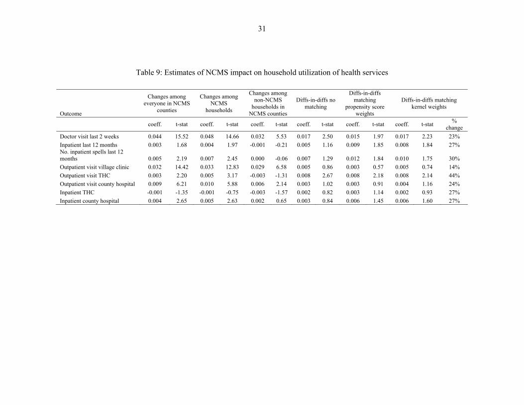
31

Table 9: Estimates of NCMS impact on household utilization of health services

Outcome

Changes among everyone in NCMS

counties

Changes among NCMS

households

Changes among non-NCMS

households in NCMS counties

Diffs-in-diffs no matching

Diffs-in-diffs matching

propensity score weights

Diffs-in-diffs matching kernel weights

coeff. t-stat coeff. t-stat coeff. t-stat coeff. t-stat coeff. t-stat coeff. t-stat % change

Doctor visit last 2 weeks 0.044 15.52 0.048 14.66 0.032 5.53 0.017 2.50 0.015 1.97 0.017 2.23 23% Inpatient last 12 months 0.003 1.68 0.004 1.97 -0.001 -0.21 0.005 1.16 0.009 1.85 0.008 1.84 27% No. inpatient spells last 12 months 0.005 2.19 0.007 2.45 0.000 -0.06 0.007 1.29 0.012 1.84 0.010 1.75 30% Outpatient visit village clinic 0.032 14.42 0.033 12.83 0.029 6.58 0.005 0.86 0.003 0.57 0.005 0.74 14% Outpatient visit THC 0.003 2.20 0.005 3.17 -0.003 -1.31 0.008 2.67 0.008 2.18 0.008 2.14 44% Outpatient visit county hospital 0.009 6.21 0.010 5.88 0.006 2.14 0.003 1.02 0.003 0.91 0.004 1.16 24% Inpatient THC -0.001 -1.35 -0.001 -0.75 -0.003 -1.57 0.002 0.82 0.003 1.14 0.002 0.93 27% Inpatient county hospital 0.004 2.65 0.005 2.63 0.002 0.65 0.003 0.84 0.006 1.45 0.006 1.60 27%

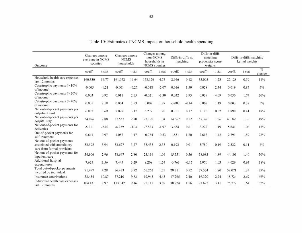
32

Table 10: Estimates of NCMS impact on household health spending

Outcome

Changes among everyone in NCMS

counties

Changes among NCMS

households

Changes among non-NCMS

households in NCMS counties

Diffs-in-diffs no matching

Diffs-in-diffs matching

propensity score weights

Diffs-in-diffs matching kernel weights

coeff. t-stat coeff. t-stat coeff. t-stat coeff. t-stat coeff. t-stat coeff. t-stat % change

Household health care expenses last 12 months 160.330 14.77 161.072 16.64 158.126 4.75 2.946 0.12 35.095 1.23 27.128 0.59 11%

Catastrophic payments (> 10% of income) -0.005 -1.21 -0.001 -0.27 -0.018 -2.07 0.016 1.59 0.028 2.34 0.019 0.87 5%

Catastrophic payments (> 20% of income) 0.003 0.92 0.011 2.65 -0.021 -3.30 0.032 3.93 0.039 4.09 0.036 1.74 20%

Catastrophic payments (> 40% of income) 0.005 2.18 0.004 1.53 0.007 1.87 -0.003 -0.64 0.007 1.19 0.003 0.37 5%

Net out-of-pocket payments per outpatient visit 6.852 3.69 7.028 3.17 6.277 1.90 0.751 0.17 2.195 0.52 1.898 0.41 18%

Net out-of-pocket payments per hospital stay 34.076 2.88 37.557 2.70 23.190 1.04 14.367 0.52 57.326 1.86 43.346 1.38 49%

Net out-of-pocket payments for deliveries -5.211 -2.02 -4.229 -1.34 -7.883 -1.97 3.654 0.61 8.222 1.19 5.841 1.06 13%

Out-of-pocket payments for self-treatment 0.641 0.97 1.087 1.47 -0.764 -0.53 1.851 1.20 2.613 1.42 2.791 1.59 78%

Net out-of-pocket payments associated with ambulatory care from formal providers

33.595 3.94 33.627 3.27 33.435 2.35 0.192 0.01 3.780 0.19 2.522 0.11 4%

Net out-of-pocket payments for inpatient care 34.906 2.96 38.667 2.80 23.116 1.04 15.551 0.56 58.083 1.89 44.109 1.40 50%

Additional hospital expenditures 7.625 3.56 7.445 3.29 8.208 1.54 -0.763 -0.15 5.070 1.03 4.029 0.93 38%

Total out-of-pocket payments incurred by individual 71.497 4.28 76.473 3.92 56.262 1.75 20.211 0.52 77.574 1.80 59.071 1.33 29%

Insurance contributions 33.454 10.87 37.210 9.83 19.945 4.45 17.265 2.40 16.320 2.74 18.724 2.69 66% Individual health care expenses last 12 months 104.431 9.97 113.342 9.16 75.118 3.89 38.224 1.56 91.622 3.41 75.777 1.64 32%

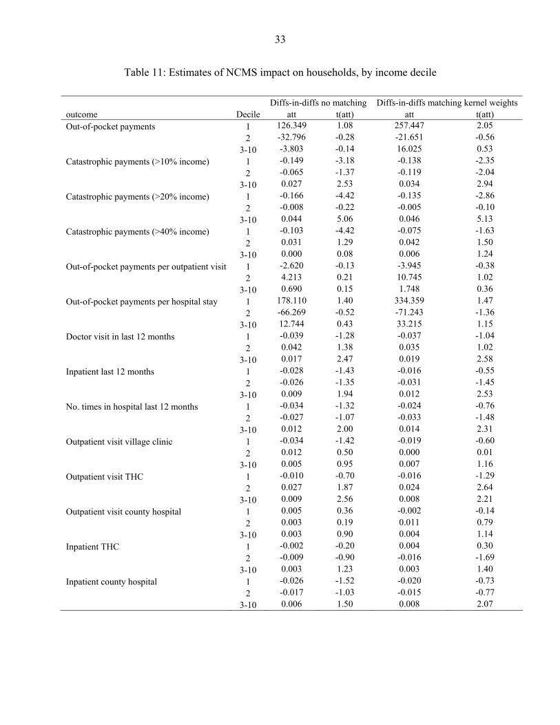
33

Table 11: Estimates of NCMS impact on households, by income decile

Diffs-in-diffs no matching Diffs-in-diffs matching kernel weights outcome Decile att t(att) att t(att) Out-of-pocket payments 1 126.349 1.08 257.447 2.05 2 -32.796 -0.28 -21.651 -0.56 3-10 -3.803 -0.14 16.025 0.53 Catastrophic payments (>10% income) 1 -0.149 -3.18 -0.138 -2.35 2 -0.065 -1.37 -0.119 -2.04 3-10 0.027 2.53 0.034 2.94 Catastrophic payments (>20% income) 1 -0.166 -4.42 -0.135 -2.86 2 -0.008 -0.22 -0.005 -0.10 3-10 0.044 5.06 0.046 5.13 Catastrophic payments (>40% income) 1 -0.103 -4.42 -0.075 -1.63 2 0.031 1.29 0.042 1.50 3-10 0.000 0.08 0.006 1.24 Out-of-pocket payments per outpatient visit 1 -2.620 -0.13 -3.945 -0.38 2 4.213 0.21 10.745 1.02 3-10 0.690 0.15 1.748 0.36 Out-of-pocket payments per hospital stay 1 178.110 1.40 334.359 1.47 2 -66.269 -0.52 -71.243 -1.36 3-10 12.744 0.43 33.215 1.15 Doctor visit in last 12 months 1 -0.039 -1.28 -0.037 -1.04 2 0.042 1.38 0.035 1.02 3-10 0.017 2.47 0.019 2.58 Inpatient last 12 months 1 -0.028 -1.43 -0.016 -0.55 2 -0.026 -1.35 -0.031 -1.45 3-10 0.009 1.94 0.012 2.53 No. times in hospital last 12 months 1 -0.034 -1.32 -0.024 -0.76 2 -0.027 -1.07 -0.033 -1.48 3-10 0.012 2.00 0.014 2.31 Outpatient visit village clinic 1 -0.034 -1.42 -0.019 -0.60 2 0.012 0.50 0.000 0.01 3-10 0.005 0.95 0.007 1.16 Outpatient visit THC 1 -0.010 -0.70 -0.016 -1.29 2 0.027 1.87 0.024 2.64 3-10 0.009 2.56 0.008 2.21 Outpatient visit county hospital 1 0.005 0.36 -0.002 -0.14 2 0.003 0.19 0.011 0.79 3-10 0.003 0.90 0.004 1.14 Inpatient THC 1 -0.002 -0.20 0.004 0.30 2 -0.009 -0.90 -0.016 -1.69 3-10 0.003 1.23 0.003 1.40 Inpatient county hospital 1 -0.026 -1.52 -0.020 -0.73 2 -0.017 -1.03 -0.015 -0.77 3-10 0.006 1.50 0.008 2.07

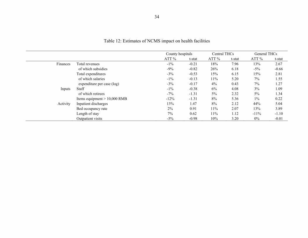
34

Table 12: Estimates of NCMS impact on health facilities

County hospitals Central THCs General THCs ATT % t-stat ATT % t-stat ATT % t-stat

Finances Total revenues -1% -0.21 18% 7.96 13% 2.67 of which subsidies -9% -0.82 26% 6.18 -5% -0.66 Total expenditures -3% -0.53 15% 6.15 15% 2.81 of which salaries -1% -0.13 11% 5.20 7% 1.55 expenditure per case (log) -3% -0.17 4% 0.43 7% 1.27

Inputs Staff -1% -0.38 6% 4.08 3% 1.09 of which retirees -7% -1.31 5% 2.32 5% 1.34 Items equipment > 10,000 RMB -12% -1.31 8% 5.36 1% 0.22

Activity Inpatient discharges 13% 1.47 8% 2.12 44% 5.04 Bed occupancy rate 2% 0.91 11% 2.07 13% 3.89 Length of stay 7% 0.62 11% 1.12 -11% -1.10 Outpatient visits -5% -0.98 10% 3.20 0% -0.01

35

References

Blumenthal, D. and W. Hsiao (2005). "Privatization and its discontents--the evolving Chinese health care system." N Engl J Med 353(11): 1165-70.

Blundell, R., L. Dearden and B. Sianesi (2005). "Evaluating the effect of education on earnings: models, methods and results from the National Child Development Survey." Journal of the Royal Statistical Society: Series A (Statistics in Society) 168(3): 473-512.

Caliendo, M. and S. Kopenig (2005). Some practical guidance for the implementation of propensity score matching. Berlin, DIW German Institute for Economic Research, Discussion Paper 485.

Carrin, G., A. Ron, H. Yang, H. Wang, T. Zhang, L. Zhaing, S. Zhang, Y. Ye, J. Chen, Q. Jiang, Z. Zhang, J. Yu and X. Li (1999). "The Reform of the Rural Cooperative Medical System in the People's Republic of China: interim experience in 14 pilot counties." Social Science & Medicine 48(7): 961-972.

Central Committee of CPC (2002). Decisions of the central committee of the communist party of China and the State Council on further strengthening rural health work. Beijing, China

Centre for Health Statistics and Information (2005). Primary Analysis Report on the Survey of New Cooperative Medical Scheme. Beijing, Ministry of Health.

Centre for Health Statistics and Information (2006). China's New Rural Cooperative Medical Scheme: Studies of Development and Effectiveness. 2005 Research Reports on Pilots of New Rural Cooperative Medical Scheme. (In Chinese.). Beijing, Ministry of Health.

Chen, S., R. Mu and M. Ravallion (2006). Are there Lasting Impacts of a Poor-Area Development Program? Washington DC, World Bank, Mimeo.

Cretin, S., N. Duan, J. Albert P. Williams, X. Gu and Y. Shi (1990). "Modeling the effect of insurance on health expenditures in the People's Republic of China." Health Services Research 25(4): 667-685.

Crump, R., J. Hotz, G. Imbens and O. Mitnik (2006). Moving the Goalposts: Addressing Limited Overlap in Estimation of Average Treatment Effects by Changing the Estimand. Berkeley, CA, UC Berkeley, Mimeo.

Escobar, M.-L. and P. Panopolou (2003). Health. Colombia : the economic foundation of peace. M. Giugale, O. Lafourcade and C. Luff. Washington, DC, World Bank: 653-707.

Frenk, J., E. Gonzalez-Pier, O. Gomez-Dantes, M. A. Lezana and F. M. Knaul (2006). "Comprehensive reform to improve health system performance in Mexico." Lancet 368(9546): 1524-34.

36

Gakidou, E., R. Lozano, E. Gonzalez-Pier, J. Abbott-Klafter, J. T. Barofsky, C. Bryson-Cahn, D. M. Feehan, D. K. Lee, H. Hernandez-Llamas and C. J. Murray (2006). "Assessing the effect of the 2001-06 Mexican health reform: an interim report card." The Lancet In Press, Corrected Proof.

Gaviria, A., C. Medina and C. Mejía (2006). Evaluating The Impact Of Health Care Reform In Colombia: From Theory To Practice. Bogota, Universidad de Los Andes-CEDE, Documentos CEDE 002682.

Grumbach, K. (2004). "Fighting Hand to Hand over Physician Workforce Policy." Health Affairs 21(5): 13-27.

Hsiao, W. and et al. (2004). "Rural Mutual Medical Care in China." The Chinese Health Economics Forthcoming.

Imbens, G. W. (2004). "Nonparametric Estimation of Average Treatment Effects under Exogeneity: A Review." Review of Economics and Statistics 86(1): 4-29.

Jalan, J. and M. Ravallion (2003). "Does Piped Water Reduce Diarrhea for Children in Rural India?" Journal of Econometrics 112(1): 153-73.

Janssens, W. (2005). Measuring Externalities in Program Evaluation: Spillover Effects of a Women's Empowerment Programme in Rural India, Tinbergen Institute Discussion Paper No. TI 05-017/2

Jowett, M., P. Contoyannis and N. D. Vinh (2003). "The impact of public voluntary health insurance on private health expenditures in Vietnam." Soc Sci Med 56(2): 333-42.

Jowett, M., A. Deolalikar and P. Martinsson (2004). "Health insurance and treatment seeking behaviour: evidence from a low-income country." Health Econ 13(9): 845-57.

Knaul, F. M., H. Arreola-Ornelas, O. Mendez-Carniado, C. Bryson-Cahn, J. Barofsky, R. Maguire, M. Miranda and S. Sesma (2006). "Evidence is good for your health system: policy reform to remedy catastrophic and impoverishing health spending in Mexico." Lancet 368(9549): 1828-41.

Knaul, F. M. and J. Frenk (2005). "Health insurance in Mexico: achieving universal coverage through structural reform." Health Aff (Millwood) 24(6): 1467-76.

Knowles, J., T. Nguyen, B. Dang, K. Nguyen, T. Tran, K. Nguyen and N. Vu (2005). Making Health Care More Affordable for the Poor: Health Financing in Vietnam. Hanoi, Medical Publishing House.

Lin, S. (2005). "Excessive Government Fee Collection in China." Contemporary Economic Policy 23(1): 91-106.

Liu, X. and A. Mills (1999). "Evaluating payment mechanisms: how can we measure unnecessary care?" Health Policy and Planning 14(4): 409-13.

37

Liu, Y., K. Rao and W. C. Hsiao (2003). "Medical expenditure and rural impoverishment in China." Journal of Health, Population & Nutrition 21(3): 216-222.

Liu, Y. L. (2004). "Development of the rural health insurance system in China." Health Policy and Planning 19(3): 159-165.

Mao, Z. (2005). Pilot NCMS Reform in China: A Review of Experiences. Unpublished manuscript (available on: www.worldbank.org/chinaruralhealth)

Ministry of Health Center for Health Statistics and Information (2004). An Analysis Report of national Health Services Survey in 2003. Beijing, Ministry of Health.

Obermann, K., M. R. Jowett, M. O. Alcantara, E. P. Banzon and C. Bodart (2006). "Social health insurance in a developing country: the case of the Philippines." Soc Sci Med 62(12): 3177-85.

Pannarunothai, S., D. Patmasiriwat and S. Srithamrongsawat (2004). "Universal health coverage in Thailand: ideas for reform and policy struggling." Health Policy 68(1): 17-30.

Panopoulu, G. and C. Velez (2001). Subsidized Health Insurance, Proxy Means Testing and the Demand for Health Care among the Poor in Colombia. Colombia Poverty Report Volume II. Washington DC, World Bank.

Ravallion, M. (2007). Evaluating Anti-Poverty Programs. Handbook of Agricultural Economics vol. 4. R. Evenson and T. Schultz. Amsterdam, North Holland.

Scott, J. (2006). Seguro Popular Incidence Analysis. Decentralized Service Delivery for the Poor Vol. II. World Bank. Washington DC, World Bank.

Sepehri, A., S. Sarma and W. Simpson (2006). "Does non-profit health insurance reduce financial burden? Evidence from the Vietnam Living Standards Survey Panel." Health Econ 15(6): 603-16.

Sepehri, A., W. Simpson and S. Sarma (2006). "The influence of health insurance on hospital admission and length of stay--the case of Vietnam." Soc Sci Med 63(7): 1757-70.

Sidel, V. (1993). "New lessons from China: equity and economics in rural health care." American Journal of Public Health 83: 1665-1666.

Smith, J. A. and P. E. Todd (2005). "Does Matching Overcome LaLonde's Critique of Nonexperimental Estimators?" Journal of Econometrics 125(1-2): 305-53.

Tao, R. and M. Liu (2005). "Urban and Rural Household Taxation in China: Measurement, Comparison and Policy Implications." Journal of the Asia Pacific Economy 10(4): 486-505.

Trivedi, P. (2003). Patterns of health care use in Vietnam: Analysis of 1998 Vietnam Living Standards Survey data. Economic Growth, Poverty and Household Welfare: Policy

38

Lessons from Vietnam. P. Glewwe, N. Agrawal and D. Dollar. Washington DC, World Bank.

Trujillo, A. J., J. E. Portillo and J. A. Vernon (2005). "The impact of subsidized health insurance for the poor: evaluating the Colombian experience using propensity score matching." Int J Health Care Finance Econ 5(3): 211-39.

Wagstaff, A. (2006). Health Insurance for the Underprivileged: Initial Impacts of Vietnam's Health Care Fund for the Poor. Washington DC, World Bank, Mimeo.

Wagstaff, A. and M. Lindelow (2005). Can insurance increase financial risk? : the curious case of health insurance in China. Washington, D.C., World Bank, Policy Research Working Paper #3741.

Wagstaff, A. and M. Pradhan (2005). Health insurance impacts on health and nonmedical consumption in a developing country. Washington, D.C., World Bank, Policy Research Working Paper 3563.

Wagstaff, A. and S. Yu (2006). "Do health sector reforms have their intended impacts? The World Bank's Health VIII Project in Gansu Province, China." Journal of Health Economics In Press, Corrected Proof.

World Bank (2004). Taking Stock of China's Rural Health Challenges. Washington DC, The World Bank

World Bank (2005). Rural Health Insurance-Rising to the Challenge. Washington DC, The World Bank

World Bank, SIDA, AusAID, Royal Netherlands Embassy and Ministry of Health of Vietnam (2001). Vietnam. Growing Healthy: A Review of Vietnam's Health Sector. Hanoi, The World Bank.

Wu, M., Z. Zhang, M. He, Y. Ruan, C. Lv, L. Tao and M. Miao (2006). Qualitative Study on the Implementation and Determinants of the New Cooperative Medical System in Rural China, Study report from WB/MOH NCMS study

Yep, R. (2004). "Can "Tax-for-Fee" Reform Reduce Rural Tension in China? The Process, Progress and Limitations." China Quarterly(177): 42-70.

Yuan, C., Z. Wang and M. Chen (1998). "Treatment and financial loss of catastrophic diseases among rural farmers." Medicine and Society 3: 627-630.

Zhan, S., L. Wang, A. Yin and E. Blas (2004). "Revenue-driven in TB control--three cases in China." Int J Health Plann Manage 19 Suppl 1: S63-78.

Zhang, X., Z. Feng and L. Zhang (2003). "Analysis on Quality of Prescription of Township Hospitals in Poor Areas." Journal of Rural Health Service Management 23(12): 33-35.

39

Zhu, N. S., Z. H. Ling, J. Shen, J. M. Lane and S. L. Hu (1989). "Factors associated with the decline of the Cooperative Medical System and barefoot doctors in rural China." Bull World Health Organ 67(4): 431-41.