Extreme bandits

Alexandra CarpentierStatistical Laboratory, CMS

University of Cambridge, UKa.carpentier@statslab.cam.ac.uk

Michal ValkoSequeL team

INRIA Lille - Nord Europe, Francemichal.valko@inria.fr

Abstract

In many areas of medicine, security, and life sciences, we want to allocate lim-ited resources to different sources in order to detect extreme values. In this paper,we study an efficient way to allocate these resources sequentially under limitedfeedback. While sequential design of experiments is well studied in bandit theory,the most commonly optimized property is the regret with respect to the maximummean reward. However, in other problems such as network intrusion detection, weare interested in detecting the most extreme value output by the sources. There-fore, in our work we study extreme regret which measures the efficiency of an al-gorithm compared to the oracle policy selecting the source with the heaviest tail.We propose the EXTREMEHUNTER algorithm, provide its analysis, and evaluateit empirically on synthetic and real-world experiments.

1 Introduction

We consider problems where the goal is to detect outstanding events or extreme values in domainssuch as outlier detection [1], security [18], or medicine [17]. The detection of extreme values isimportant in many life sciences, such as epidemiology, astronomy, or hydrology, where, for example,we may want to know the peak water flow. We are also motivated by network intrusion detectionwhere the objective is to find the network node that was compromised, e.g., by seeking the onecreating the most number of outgoing connections at once. The search for extreme events is typicallystudied in the field of anomaly detection, where one seeks to find examples that are far away fromthe majority, according to some problem-specific distance (cf. the surveys [8, 16]).

In anomaly detection research, the concept of anomaly is ambiguous and several definitions ex-ist [16]: point anomalies, structural anomalies, contextual anomalies, etc. These definitions areoften followed by heuristic approaches that are seldom analyzed theoretically. Nonetheless, thereexist some theoretical characterizations of anomaly detection. For instance, Steinwart et al. [19]consider the level sets of the distribution underlying the data, and rare events corresponding to rarelevel sets are then identified as anomalies. A very challenging characteristic of many problems inanomaly detection is that the data emitted by the sources tend to be heavy-tailed (e.g., network traf-fic [2]) and anomalies come from the sources with the heaviest distribution tails. In this case, rarelevel sets of [19] correspond to distributions’ tails and anomalies to extreme values. Therefore, wefocus on the kind of anomalies that are characterized by their outburst of events or extreme values,as in the setting of [22] and [17].

Since in many cases, the collection of the data samples emitted by the sources is costly, it is im-portant to design adaptive-learning strategies that spend more time sampling sources that have ahigher risk of being abnormal. The main objective of our work is the active allocation of the sam-pling resources for anomaly detection, in the setting where anomalies are defined as extreme values.Specifically, we consider a variation of the common setting of minimal feedback also known asthe bandit setting [14]: the learner searches for the most extreme value that the sources output byprobing the sources sequentially. In this setting, it must carefully decide which sources to observe

1

because it only receives the observation from the source it chooses to observe. As a consequence,it needs to allocate the sampling time efficiently and should not waste it on sources that do not havean abnormal character. We call this specific setting extreme bandits, but it is also known as max-kproblem [9, 21, 20]. We emphasize that extreme bandits are poles apart from classical bandits, wherethe objective is to maximize the sum of observations [3]. An effective algorithm for the classicalbandit setting should focus on the source with the highest mean, while an effective algorithm for theextreme bandit problem should focus on the source with the heaviest tail. It is often the case thata heavy-tailed source has a small mean, which implies that the classical bandit algorithms performpoorly for the extreme bandit problem.

The challenging part of our work dwells in the active sampling strategy to detect the heaviest tailunder the limited bandit feedback. We proffer EXTREMEHUNTER, a theoretically founded algo-rithm, that sequentially allocates the resources in an efficient way, for which we prove performanceguarantees. Our algorithm is efficient under a mild semi-parametric assumption common in ex-treme value theory, while known results by [9, 21, 20] for the extreme bandit problem only hold ina parametric setting (see Section 4 for a detailed comparison).

2 Learning model for extreme bandits

In this section, we formalize the active (bandit) setting and characterize the measure of performancefor any algorithm π. The learning setting is defined as follows. Every time step, each of the K arms(sources) emits a sample Xk,t ∼ Pk, unknown to the learner. The precise characteristics of Pk aredefined in Section 3. The learner π then chooses some arm It and then receives only the sampleXIt,t. The performance of π is evaluated by the most extreme value found and compared to themost extreme value possible. We define the reward of a learner π as:

Gπn = maxt≤n

XIt,t

The optimal oracle strategy is the one that chooses at each time the arm with the highest potentialrevealing the highest value, i.e., the arm ∗ with the heaviest tail. Its expected reward is then:

E [G∗n] = maxk≤K

E[maxt≤n

Xk,t

]The goal of learner π is to get as close as possible to the optimal oracle strategy. In other words, theaim of π is to minimize the expected extreme regret:

Definition 1. The extreme regret in the bandit setting is defined as:

E [Rπn] = E [G∗n]− E [Gπn] = maxk≤K

E[maxt≤n

Xk,t

]− E

[maxt≤n

XIt,t

]

3 Heavy-tailed distributions

In this section, we formally define our observation model. Let X1, . . . , Xn be n i.i.d. observationsfrom a distribution P . The behavior of the statistic maxi≤nXi is studied by extreme value theory.One of the main results is the Fisher-Tippett-Gnedenko theorem [11, 12] that characterizes the lim-iting distribution of this maximum as n converges to infinity. Specifically, it proves that a rescaledversion of this maximum converges to one of the three possible distributions: Gumbel, Frechet, orWeibull. This rescaling factor depends on n. To be concise, we write “maxi≤nXi converges to adistribution” to refer to the convergence of the rescaled version to a given distribution. The Gum-bel distribution corresponds to the limiting distribution of the maximum of ‘not too heavy tailed’distributions, such as sub-Gaussian or sub-exponential distributions. The Weibull distribution co-incides with the behaviour of the maximum of some specific bounded random variables. Finally,the Frechet distribution corresponds to the limiting distribution of the maximum of heavy-tailedrandom variables. As many interesting problems concern heavy-tailed distributions, we focus onFrechet distributions in this work. The distribution function of a Frechet random variable is definedfor x ≥ m, and for two parameters α, s as:

P (x) = exp{−(x−ms

)α}.

2

In this work, we consider positive distributions P : [0,∞) → [0, 1]. For α > 0, the Fisher-Tippett-Gnedenko theorem also states that the statement ‘P converges to an α-Frechet distribution’is equivalent to the statement ‘1−P is a−α regularly varying function in the tail’. These statementsare slightly less restrictive than the definition of approximately α-Pareto distributions1, i.e., that thereexists C such that P verifies:

limx→∞

|1− P (x)− Cx−α|x−α

= 0, (1)

or equivalently that P (x) = 1 − Cx−α + o(x−α). If and only if 1 − P is −α regularly varying inthe tail, then the limiting distribution of maxiXi is an α-Frechet distribution. The assumption of−α regularly varying in the tail is thus the weakest possible assumption that ensures that the (prop-erly rescaled) maximum of samples emitted by a heavy tailed distributions has a limit. Therefore,the very related assumption of approximate Pareto is almost minimal, but it is (provably) still notrestrictive enough to ensure a convergence rate. For this reason, it is natural to introduce an assump-tion that is slightly stronger than (1). In particular, we assume, as it is common in the extreme valueliterature, a second order Pareto condition also known as the Hall condition [13].Definition 2. A distribution P is (α, β, C,C ′)-second order Pareto (α, β, C,C ′ > 0) if for x ≥ 0:∣∣1− P (x)− Cx−α

∣∣ ≤ C ′x−α(1+β)

By this definition, P (x) = 1 − Cx−α + O(x−α(1+β)

), which is stronger than the assumption

P (x) = 1− Cx−α + o(x−α), but similar for small β.

Remark 1. In the definition above, β defines the rate of the convergence (when x diverges to infinity)of the tail of P to the tail of a Pareto distribution 1 − Cx−α. The parameter α characterizes theheaviness of the tail: The smaller the α, the heavier the tail. In the reminder of the paper, we will betherefore concerned with learning the α and identifying the smallest one among the sources.

4 Related work

There is a vast body of research in offline anomaly detection which looks for examples that deviatefrom the rest of the data, or that are not expected from some underlying model. A comprehensivereview of many anomaly detection approaches can be found in [16] or [8]. There has been also somework in active learning for anomaly detection [1], which uses a reduction to classification. In onlineanomaly detection, most of the research focuses on studying the setting where a set of variables ismonitored. A typical example is the monitoring of cold relief medications, where we are interestedin detecting an outbreak [17]. Similarly to our focus, these approaches do not look for outliers in abroad sense but rather for the unusual burst of events [22].

In the extreme values settings above, it is often assumed, that we have full information about eachvariable. This is in contrast to the limited feedback or a bandit setting that we study in our work.There has been recently some interest in bandit algorithms for heavy-tailed distributions [4]. How-ever the goal of [4] is radically different from ours as they maximize the sum of rewards and notthe maximal reward. Bandit algorithms have been already used for network intrusion detection [15],but they typically consider classical or restless setting. [9, 21, 20] were the first to consider theextreme bandits problem, where our setting is defined as the max-k problem. [21] and [9] con-sider a fully parametric setting. The reward distributions are assumed to be exactly generalizedextreme value distributions. Specifically, [21] assumes that the distributions are exactly Gumbel,P (x) = exp(−(x − m)/s)), and [9], that the distributions are exactly of Gumbel or FrechetP (x) = exp(−(x − m)α/(sα))). Provided that these assumptions hold, they propose an algo-rithm for which the regret is asymptotically negligible when compared to the optimal oracle reward.These results are interesting since they are the first for extreme bandits, but their parametric assump-tion is unlikely to hold in practice and the asymptotic nature of their bounds limits their impact.Interestingly, the objective of [20] is to remove the parametric assumptions of [21, 9] by offeringthe THRESHOLDASCENT algorithm. However, no analysis of this algorithm for extreme bandits isprovided. Nonetheless, to the best of our knowledge, this is the closest competitor for EXTREME-HUNTER and we empirically compare our algorithm to THRESHOLDASCENT in Section 7.

1We recall the definition of the standard Pareto distribution as a distribution P , where for some constants αand C, we have that for x ≥ C1/α, P = 1− Cx−α.

3

In this paper we also target the extreme bandit setting, but contrary to [9, 21, 20], we only make asemi-parametric assumption on the distribution; the second order Pareto assumption (Definition 2),which is standard in extreme value theory (see e.g., [13, 10]). This is light-years better and sig-nificantly weaker than the parametric assumptions made in the prior works for extreme bandits.Furthermore, we provide a finite-time regret bound for our more general semi-parametric setting(Theorem 2), while the prior works only offer asymptotic results. In particular, we provide an up-per bound on the rate at which the regret becomes negligible when compared to the optimal oraclereward (Definition 1).

5 Extreme Hunter

In this section, we present our main results. In particular, we present the algorithm and the maintheorem that bounds its extreme regret. Before that, we first provide an initial result on the expecta-tion of the maximum of second order Pareto random variables which will set the benchmark for theoracle regret. We first characterize the expectation of the maximum of second order Pareto distribu-tions. The following lemma states that the expectation of the maximum of i.i.d. second order Paretosamples is equal, up to a negligible term, to the expectation of the maximum of i.i.d. Pareto samples.This result is crucial for assessing the benchmark for the regret, in particular the expected value ofthe maximal oracle sample. Theorem 1 is based on Lemma 3, both provided in the appendix.

Theorem 1. Let X1, . . . , Xn be n i.i.d. samples drawn according to (α, β, C,C ′)-second orderPareto distribution P (see Definition 2). If α > 1, then:∣∣∣E(max

iXi)− (nC)1/αΓ

(1− 1

α

)∣∣∣ ≤ 4D2

n (nC)1/α +2C′Dβ+1

Cβ+1nβ(nC)1/α +B = o

((nC)

1/α),

where D2, D1+β > 0 are some universal constants, and B is defined in the appendix (9).

Theorem 1 implies that the optimal strategy in hindsight attains the following expected reward:

E [G∗n] ≈ maxk

[(Ckn)

1/αk Γ(1− 1

α

)]Algorithm 1 EXTREMEHUNTER

Input:K: number of armsn: time horizonb: where b ≤ βk for all k ≤ KN : minimum number of pulls of each arm

Initialize:Tk ← 0 for all k ≤ Kδ ← exp(− log2 n)/(2nK)

Run:for t = 1 to n do

for k = 1 to K doif Tk ≤ N thenBk,t ←∞

elseestimate hk,t that verifies (2)estimate Ck,t using (3)update Bk,t using (5) with (2) and (4)

end ifend forPlay arm kt ← arg maxk Bk,tTkt ← Tkt + 1

end for

Our objective is therefore to find a learner πsuch that E [G∗n] − E [Gπn] is negligible whencompared to E[G∗n], i.e., when compared to(nC∗)1/α∗Γ

(1− 1

α∗

)≈ n1/α∗ where ∗ is the

optimal arm.

From the discussion above, we know that theminimization of the extreme regret is linkedwith the identification of the arm with the heav-iest tail. Our EXTREMEHUNTER algorithm isbased on a classical idea in bandit theory: op-timism in the face of uncertainty. Our strat-egy is to estimate E [maxt≤nXk,t] for any kand to pull the arm which maximizes its up-per bound. From Definition 2, the estimationof this quantity relies heavily on an efficient es-timation of αk and Ck, and on associated confi-dence widths. This topic is a classic problem inextreme value theory, and such estimators existprovided that one knows a lower bound b on βk[10, 6, 7]. From now on we assume that a con-stant b > 0 such that b ≤ mink βk is knownto the learner. As we argue in Remark 2, thisassumption is necessary .

Since our main theoretical result is a finite-time upper bound, in the following exposition we care-fully describe all the constants and stress what quantities they depend on. Let Tk,t be the number ofsamples drawn from arm k at time t. Define δ = exp(− log2 n)/(2nK) and consider an estimator

4

hk,t of 1/αk at time t that verifies the following condition with probability 1−δ, for Tk,t larger thansome constant N2 that depends only on αk, Ck, C ′ and b:∣∣∣ 1

αk− hk,t

∣∣∣ ≤ D√log(1/δ)T−b/(2b+1)k,t = B1(Tk,t), (2)

where D is a constant that also depends only on αk, Ck, C ′, and b. For instance, the estimatorin [6] (Theorem 3.7) verifies this property and provides D and N2 but other estimators are possible.Consider the associated estimator for Ck:

Ck,t = T1/(2b+1)k,t

1

Tk,t

Tk,t∑u=1

1{Xk,u ≥ T

hk,t/(2b+1)k,t

} (3)

For this estimator, we know [7] with probability 1− δ that for Tk,t ≥ N2:∣∣∣Ck − Ck,t∣∣∣ ≤ E√log(Tk,t/δ) log(Tk,t)T−b/(2b+1)k,T = B2(Tk,t), (4)

where E is derived in [7] in the proof of Theorem 2. Let N = max(A log(n)2(2b+1)/b, N2

)where

A depends on (αk, Ck)k, b,D,E, and C ′, and is such that:

max (2B1(N), 2B2(N)/Ck) ≤ 1, N ≥ (2D log2 n)(2b+1)/b, and N >

(2D√

log(n)2

1−maxk 1/αk

)(2b+1)/b

This inspires Algorithm 1, which first pulls each arm N times and then, at each time t > KN , pullsthe arm that maximizes Bk,t, which we define as:((

Ck,t +B2 (Tk,t))n)hk,t+B1(Tk,t)

Γ(hk,t, B1 (Tk,t)

), (5)

where Γ(x, y) = Γ(1− x− y), where we set Γ = Γ for any x > 0 and +∞ otherwise.

Remark 2. A natural question is whether it is possible to learn βk as well. In fact, this is not possiblefor this model and a negative result was proved by [7]. The result states that in this setting it is notpossible to test between two fixed values of β uniformly over the set of distributions. Thereupon, wedefine b as a lower bound for all βk. With regards to the Pareto distribution, β =∞ corresponds tothe exact Pareto distribution, while β = 0 for such distribution that is not (asymptotically) Pareto.

We show that this algorithm meets the desired properties. The following theorem states our mainresult by upper-bounding the extreme regret of EXTREMEHUNTER.

Theorem 2. Assume that the distributions of the arms are respectively (αk, βk, Ck, C′) second

order Pareto (see Definition 2) with mink αk > 1. If n ≥ Q, the expected extreme regret of EX-TREMEHUNTER is bounded from above as:

E [Rn] ≤ L(nC∗)1/α∗(Kn log(n)(2b+1)/b + n− log(n)(1−1/α∗) + n−b/((b+1)α∗)

)= E [G∗n] o(1),

where L,Q > 0 are some constants depending only on (αk, Ck)k, C′, and b (Section 6).

Theorem 2 states that the EXTREMEHUNTER strategy performs almost as well as the best (oracle)strategy, up to a term that is negligible when compared to the performance of the oracle strategy.Indeed, the regret is negligible when compared to (nC∗)1/α∗ , which is the order of magnitude of theperformance of the best oracle strategy E [G∗n] = maxk≤K E [maxt≤nXk,t]. Our algorithm thusdetects the arm that has the heaviest tail.

For n large enough (as a function of (αk, βk, Ck)k, C′ and K), the two first terms in the regret

become negligible when compared to the third one, and the regret is then bounded as:

E [Rn] ≤ E [G∗n]O(n−b/((b+1)α∗)

)We make two observations: First, the larger the b, the tighter this bound is, since the model is thencloser to the parametric case. Second, smaller α∗ also tightens the bound, since the best arm is thenvery heavy tailed and much easier to recognize.

5

6 Analysis

In this section, we prove an upper bound on the extreme regret of Algorithm 1 stated in Theorem 2.Before providing the detailed proof, we give a high-level overview and the intuitions.

In Step 1, we define the (favorable) high probability event ξ of interest, useful for analyzing themechanism of the bandit algorithm. In Step 2, given ξ, we bound the estimates of αk and Ck, anduse them to bound the main upper confidence bound. In Step 3, we upper-bound the number of pullsof each suboptimal arm: we prove that with high probability we do not pull them too often. Thisenables us to guarantee that the number of pulls of the optimal arms ∗ is on ξ equal to n up to anegligible term.

The final Step 4 of the proof is concerned with using this lower bound on the number of pulls ofthe optimal arm in order to lower bound the expectation of the maximum of the collected samples.Such step is typically straightforward in the classical (mean-optimizing) bandits by the linearity ofthe expectation. It is not straightforward in our setting. We therefore prove Lemma 2, in which weshow that the expected value of the maximum of the samples in the favorable event ξ will be not toofar away from the one that we obtain without conditioning on ξ.

Step 1: High probability event. In this step, we define the favorable event ξ. We setδ

def= exp(− log2n)/(2nK) and consider the event ξ such that for any k ≤ K, N ≤ T ≤ n:∣∣∣ 1αk− hk(T )

∣∣∣ ≤ D√log(1/δ)T−b/(2b+1),∣∣∣Ck − Ck(T )∣∣∣ ≤ E√log(T/δ)T−b/(2b+1),

where hk(T ) and Ck(T ) are the estimates of 1/αk and Ck respectively using the first T samples.Notice, they are not the same as hk,t and Ck,t which are the estimates of the same quantities at timet for the algorithm, and thus with Tk,t samples. The probability of ξ is larger than 1 − 2nKδ by aunion bound on (2) and (4).

Step 2: Bound on Bk,t. The following lemma holds on ξ for upper- and lower-bounding Bk,t.Lemma 1. (proved in the appendix) On ξ, we have that for any k ≤ K, and for Tk,t ≥ N :

(Ckn)1αk Γ

(1− 1

αk

)≤ Bk,t≤(Ckn)

1αk Γ

(1− 1

αk

)(1 + F log(n)

√log(n/δ)T

−b/(2b+1)k,t

)(6)

Step 3: Upper bound on the number of pulls of a suboptimal arm. We proceed by using thebounds on Bk,t from the previous step to upper-bound the number of suboptimal pulls. Let ∗ be thebest arm. Assume that at round t, some arm k 6= ∗ is pulled. Then by definition of the algorithmB∗,t ≤ Bk,t, which implies by Lemma 1:

(C∗n)1/α∗

Γ(1− 1

α∗

)≤ (Ckn)

1/αk Γ(

1− 1αk

)(1 + F log(n)

√log(n/δ)T

−b/(2b+1)k,t

)Rearranging the terms we get:

(C∗n)1/α∗

Γ(1− 1

α∗

)(Ckn)

1/αk Γ(1− 1

αk

) ≤ 1 + F log(n)√

log(n/δ)T−b/(2b+1)k,t (7)

We now define ∆k which is analogous to the gap in the classical bandits:

∆k =(C∗n)

1/α∗Γ(1− 1

α∗

)(Ckn)

1/αk Γ(1− 1

αk

) − 1

Since Tk,t ≤ n, (7) implies for some problem dependent constants G and G′ dependent only on(αk, Ck)k, C

′ and b, but independent of δ that:

Tk,t ≤ N +G′(

log2n log(n/δ)∆2k

)(2b+1)/(2b)

≤ N +G(log2n log(n/δ)

)(2b+1)(2b)

6

This implies that number T ∗ of pulls of arm ∗ is with probability 1− δ′, at least

n−∑k 6=∗

G(log2n log(2nK/δ′)

)(2b+1)/(2b) −KN,

where δ′ = 2nKδ. Since n is larger than

Q ≥ 2KN + 2GK(log2n log (2nK/δ′)

)(2b+1)/(2b),

we have that T ∗ ≥ n2 as a corollary.

Step 4: Bound on the expectation. We start by lower-bounding the expected gain:

E[Gn]=E[maxt≤n

XIt,Tk,t

]≥E

[maxt≤n

XIt,Tk,t1{ξ}]≥E

[maxt≤n

X∗,T∗,t1{ξ}]

=E[maxi≤T∗

Xi1{ξ}]

The next lemma links the expectation of maxt≤T∗ X∗,t with the expectation of maxt≤T∗ X∗,t1{ξ}.

Lemma 2. (proved in the appendix) Let X1, . . . , XT be i.i.d. samples from an (α, β, C,C ′)-secondorder Pareto distribution F . Let ξ′ be an event of probability larger than 1 − δ. Then for δ < 1/2

and for T ≥ Q large enough so that cmax(1/T, 1/T β

)≤ 1/4 for a given constant c > 0, that

depends only on C,C ′ and β, and also for T ≥ log(2) max(C (2C ′)

1/β, 8 log (2)

):

E[maxt≤T

Xt1{ξ}]≥ (TC)

1/αΓ(1− 1

α

)−(4 + 8

α−1

)(TC)

1/αδ1−1/α

− 2(

4D2

T (TC)1/α

+2C′D1+β

C1+βTβ(TC)

1/α+B

).

Since n is large enough so that 2n2Kδ′ = 2n2K exp(− log2n

)≤ 1/2, where δ′ = exp

(− log2n

),

and the probability of ξ is larger than 1− δ′, we can use Lemma 2 for the optimal arm:

E[

maxt≤T∗

X∗,t1{ξ}]≥(T ∗C∗)

1α∗

[Γ(1− 1

α∗

)−(4+ 8

α−1

)δ′1−

1α∗ − 8D2

T∗ −4C′Dmax

(C∗)1+b(T∗)b− 2B

(T∗C∗)1α∗

],

where Dmaxdef=maxiD1+βi . Using Step 3, we bound the above with a function of n. In particular,

we lower-bound the last three terms in the brackets using T ∗ ≥ n2 and the (T ∗C∗)1/α∗ factor as:

(T ∗C∗)1/α∗ ≥ (nC∗)1/α∗(

1− GKn

(log(2n2K/δ′)

) 2b+12b −KN

n

)We are now ready to relate the lower bound on the gain of EXTREMEHUNTER with the upper boundof the gain of the optimal policy (Theorem 1), which brings us the upper bound for the regret:

E [Rn] = E [G∗n]− E [Gn] ≤ E [G∗n]− E[maxi≤T∗

Xi

]≤ E [G∗n]− E

[maxt≤T∗

X∗,t1{ξ}]

≤ H(nC∗)1/α∗(

1n+ 1

(nC∗)b+GK

n

(log(2n2K/δ′)

) 2b+12b + KN

n + δ′1−1/α∗ + B(nC∗)1/α∗

),

where H is a constant that depends on (αk, Ck)k, C′, and b. To bound the last term, we use the

definition of B (9) to get the n−β∗/((β∗+1)α∗) term, upper-bounded by n−b/((b+1)α∗) as b ≤ β∗.

Notice that this final term also eats up n−1 and n−b terms since b/((b+ 1)α∗) ≤ min(1, b).

We finish by using δ′ = exp(− log2n

)and grouping the problem-dependent constants into L to get

the final upper bound:

E [Rn] ≤ L(nC∗)1/α∗(Kn log(n)(2b+1)/b + n− log(n)(1−1/α∗) + n−b/((b+1)α∗)

)

7

0 1000 2000 3000 4000 5000 6000 7000 8000 9000 100000

1000

2000

3000

4000

5000

6000

7000

8000

9000

10000

time t

extr

eme

regr

et

Comparison of extreme bandit strategies (K=3)

ExtremeHunterUCBThresholdAscent

0 1000 2000 3000 4000 5000 6000 7000 8000 9000 100000

500

1000

1500

2000

2500

time t

extr

eme

regr

et

Comparison of extreme bandit strategies (K=3)

ExtremeHunterUCBThresholdAscent

0 1000 2000 3000 4000 5000 6000 7000 8000 9000 100000

50

100

150

200

250

time t

extr

eme

regr

et

Comparison of extreme bandit strategies on the network data K=5

ExtremeHunter

UCB

ThresholdAscent

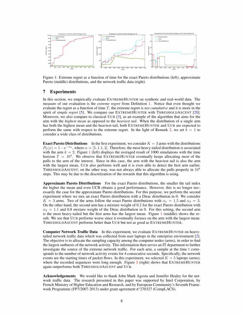
Figure 1: Extreme regret as a function of time for the exact Pareto distributions (left), approximatePareto (middle) distributions, and the network traffic data (right).

7 ExperimentsIn this section, we empirically evaluate EXTREMEHUNTER on synthetic and real-world data. Themeasure of our evaluation is the extreme regret from Definition 1. Notice that even thought weevaluate the regret as a function of time T , the extreme regret is not cumulative and it is more in thespirit of simple regret [5]. We compare our EXTREMEHUNTER with THRESHOLDASCENT [20].Moreover, we also compare to classical UCB [3], as an example of the algorithm that aims for thearm with the highest mean as opposed to the heaviest tail. When the distribution of a single armhas both the highest mean and the heaviest-tail, both EXTREMEHUNTER and UCB are expected toperform the same with respect to the extreme regret. In the light of Remark 2, we set b = 1 toconsider a wide class of distributions.

Exact Pareto Distributions In the first experiment, we considerK = 3 arms with the distributionsPk(x) = 1−x−αk , where α = [5, 1.1, 2]. Therefore, the most heavy-tailed distribution is associatedwith the arm k = 2. Figure 1 (left) displays the averaged result of 1000 simulations with the timehorizon T = 104. We observe that EXTREMEHUNTER eventually keeps allocating most of thepulls to the arm of the interest. Since in this case, the arm with the heaviest tail is also the armwith the largest mean, UCB also performs well and it is even able to detect the best arm earlier.THRESHOLDASCENT, on the other way, was not always able to allocate the pulls properly in 104

steps. This may be due to the discretization of the rewards that this algorithm is using.

Approximate Pareto Distributions For the exact Pareto distributions, the smaller the tail indexthe higher the mean and even UCB obtains a good performance. However, this is no longer nec-essarily the case for the approximate Pareto distributions. For this purpose, we perform the secondexperiment where we mix an exact Pareto distribution with a Dirac distribution in 0. We considerK = 3 arms. Two of the arms follow the exact Pareto distributions with α1 = 1.5 and α3 = 3.On the other hand, the second arm has a mixture weight of 0.2 for the exact Pareto distribution withα2 = 1.1 and 0.8 mixture weight of the Dirac distribution in 0. For this setting, the second armis the most heavy-tailed but the first arms has the largest mean. Figure 1 (middle) shows the re-sult. We see that UCB performs worse since it eventually focuses on the arm with the largest mean.THRESHOLDASCENT performs better than UCB but not as good as EXTREMEHUNTER.

Computer Network Traffic Data In this experiment, we evaluate EXTREMEHUNTER on heavy-tailed network traffic data which was collected from user laptops in the enterprise environment [2].The objective is to allocate the sampling capacity among the computer nodes (arms), in order to findthe largest outbursts of the network activity. This information then serves an IT department to furtherinvestigate the source of the extreme network traffic. For each arm, a sample at the time t corre-sponds to the number of network activity events for 4 consecutive seconds. Specifically, the networkevents are the starting times of packet flows. In this experiment, we selected K = 5 laptops (arms),where the recorded sequences were long enough. Figure 1 (right) shows that EXTREMEHUNTERagain outperforms both THRESHOLDASCENT and UCB.

Acknowledgements We would like to thank John Mark Agosta and Jennifer Healey for the net-work traffic data. The research presented in this paper was supported by Intel Corporation, byFrench Ministry of Higher Education and Research, and by European Community’s Seventh Frame-work Programme (FP7/2007-2013) under grant agreement no270327 (CompLACS).

8

References

[1] Naoki Abe, Bianca Zadrozny, and John Langford. Outlier Detection by Active Learning. InProceedings of the 12th ACM SIGKDD International Conference on Knowledge Discovery andData Mining, pages 504–509, 2006.

[2] John Mark Agosta, Jaideep Chandrashekar, Mark Crovella, Nina Taft, and Daniel Ting. Mix-ture models of endhost network traffic. In IEEE Proceedings of INFOCOM,, pages 225–229.

[3] Peter Auer, Nicolo Cesa-Bianchi, and Paul Fischer. Finite-time Analysis of the MultiarmedBandit Problem. Machine Learning, 47(2-3):235–256, 2002.

[4] Sebastien Bubeck, Nicolo Cesa-Bianchi, and Gabor Lugosi. Bandits With Heavy Tail. Infor-mation Theory, IEEE Transactions on, 59(11):7711–7717, 2013.

[5] Sebastien Bubeck, Remi Munos, and Gilles Stoltz. Pure Exploration in Multi-armed BanditsProblems. Algorithmic Learning Theory, pages 23–37, 2009.

[6] Alexandra Carpentier and Arlene K. H. Kim. Adaptive and minimax optimal estimation of thetail coefficient. Statistica Sinica, 2014.

[7] Alexandra Carpentier and Arlene K. H. Kim. Honest and adaptive confidence interval for thetail coefficient in the Pareto model. Electronic Journal of Statistics, 2014.

[8] Varun Chandola, Arindam Banerjee, and Vipin Kumar. Anomaly detection: A survey. ACMComput. Surv., 41(3):15:1–15:58, July 2009.

[9] Vincent A. Cicirello and Stephen F. Smith. The max k-armed bandit: A new model of explo-ration applied to search heuristic selection. AAAI Conference on Artificial Intelligence, 2005.

[10] Laurens de Haan and Ana Ferreira. Extreme Value Theory: An Introduction. Springer Seriesin Operations Research and Financial Engineering. Springer, 2006.

[11] Ronald Aylmer Fisher and Leonard Henry Caleb Tippett. Limiting forms of the frequencydistribution of the largest or smallest member of a sample. Mathematical Proceedings of theCambridge Philosophical Society, 24:180, 1928.

[12] Boris Gnedenko. Sur la distribution limite du terme maximum d’une serie aleatoire. TheAnnals of Mathematics, 44(3):423–453, 1943.

[13] Peter Hall and Alan H. Welsh. Best Attainable Rates of Convergence for Estimates of Param-eters of Regular Variation. The Annals of Statistics, 12(3):1079–1084, 1984.

[14] Tze L. Lai and Herbert Robbins. Asymptotically efficient adaptive allocation rules. Advancesin Applied Mathematics, 6(1):4–22, 1985.

[15] Keqin Liu and Qing Zhao. Dynamic Intrusion Detection in Resource-Constrained Cyber Net-works. In IEEE International Symposium on Information Theory Proceedings, 2012.

[16] Markos Markou and Sameer Singh. Novelty detection: a review, part 1: statistical approaches.Signal Process., 83(12):2481–2497, 2003.

[17] Daniel B. Neill and Gregory F. Cooper. A multivariate Bayesian scan statistic for early eventdetection and characterization. Machine Learning, 79:261–282, 2010.

[18] Carey E. Priebe, John M. Conroy, David J. Marchette, and Youngser Park. Scan Statistics onEnron Graphs. In Computational and Mathematical Organization Theory, volume 11, pages229–247, 2005.

[19] Ingo Steinwart, Don Hush, and Clint Scovel. A Classification Framework for Anomaly Detec-tion. Journal of Machine Learning Research, 6:211–232, 2005.

[20] Matthew J. Streeter and Stephen F. Smith. A Simple Distribution-Free Approach to the Maxk-Armed Bandit Problem. In Principles and Practice of Constraint Programming, volume4204, pages 560–574, 2006.

[21] Matthew J. Streeter and Stephen F. Smith. An Asymptotically Optimal Algorithm for the Maxk-Armed Bandit Problem. In AAAI Conference on Artificial Intelligence Intelligence, pages135–142, 2006.

[22] Ryan Turner, Zoubin Ghahramani, and Steven Bottone. Fast online anomaly detection usingscan statistics. IEEE Workshop on Machine Learning for Signal Processing, 2010.

9

A Proof of Lemma 3

Lemma 3. Assume that X1, . . . , XT are T i.i.d. samples drawn according to (α, β, C,C ′)-secondorder Pareto distribution, then for any x ≥ B:∣∣∣P(max

iXi ≤ x

)−exp

(−TCx−α

)∣∣∣ ≤Mexp(−TCx−α

)where M =

4

T

(TCx−α

)2+

2C ′

Cβ+1T β(TCx−α

)β+1, (8)

where B is defined as:

B = max(

(2C ′/C)1/(αβ)

, (8C)1/α

, (2TC ′)1/(α(1+β))). (9)

Alternatively, let u ∈ (0, 1). When T ≥ log(1/u)Bα/C:∣∣∣P(maxiXi ≤ (TC/ log (1/u))

1/α)− u∣∣∣ ≤ u( 4

Tlog(1/u)2 +

2C ′

Cβ+1T β(log(1/u))1+β

)= u×O

(1

Tlog (1/u)

2+

1

T βlog (1/u)

1+β

)Proof. Consider x ≥ B. Since the samples are i.i.d., we are going to study the following quantity:2

P(maxiXi ≤ x) = P (x)T (10)

Since P is a second order Pareto, we have for any x ≥ 0:

1− Cx−α − C ′x−α(1+β) ≤ P (x) ≤ 1− Cx−α + C ′x−α(1+β) (11)

Since x ≥ B, we deduce from the first two terms in (9) that:

Cx−α ≥ 2C ′x−α(1+β) and 2Cx−α ≤ 1/4 (12)

Let cx be the quantity that depends on x and that is such that P (x) = 1 − Ccxx−α. With suchdefinition we know by (11) and further by the second inequality in (12) that:

|cx − 1| ≤ C ′x−αβ

C≤ 1/2. (13)

Let y = Ccxx−α. By (12) and (13) we get that y ∈ [0, 1

2 ]. For any y ∈ [0, 12 ], we have:

−y − y2 ≤ log(1− y) ≤ −yTaking the exponential, setting y = Ccxx

−α, and raising to the T -th power, we obtain:

exp(−T

(Ccxx

−α)2) ≤ (1− Ccxx−α)T

exp (−T (Ccxx−α))≤ 1,

which by (10), the definition of cx, and both inequalities in (11) yields:

exp(−T

(2Cx−α

)2 − TC ′x−α(1+β))≤ P(maxiXi ≤ x)

exp(−TCx−α)≤ exp

(TC ′x−α(1+β)

)After multiplication and subtraction of exp(−TCx−α):

exp(−TCx−α

) (exp

(−4T (Cx−α)2 − TC ′x−α(1+β)

)− 1)

≤ P(

maxiXi ≤ x

)− exp

(−TCx−α

)≤ exp

(−TCx−α

) (exp

(TC ′x−α(1+β)

)− 1)

2Notice that uT means ‘u to the power of T ’ and not ‘u transposed’.

10

We will now simplify the exp(y) − 1 terms in the previous inequality. For any y such that y ∈(0, 1/2), we have exp(y) − 1 ≤ 2y and for any y ∈ R we have that y ≤ exp(y) − 1. In particular,this implies whenever x ≥ B ≥ (2TC ′)1/(α(1+β)), which is the third term in (9):

exp(−TCx−α

) (−4T (Cx−α)2 − TC ′x−α(1+β)

)≤ P

(maxiXi ≤ x

)− exp

(−TCx−α

)≤ exp

(−TCx−α

) (2TC ′x−α(1+β)

)This implies that for any x ≥ B and M as defined in (8):∣∣∣P (max

iXi ≤ x

)− exp

(−TCx−α

)∣∣∣ ≤M exp(−TCx−α

)We now simply reparametrize this upper bound by setting:

u = exp(−TCx−α)

Then u ∈ (0, 1) and x = (TC/ log (1/u))1/α

. Then x is larger than B as soon as T is larger thanlog(1/u)Bα/C. It follows that for such T , by the reparametrization in u, the rate of convergence ofthe distribution to a Frechet distribution:∣∣∣P(max

iXi ≤ (TC/ log (1/u))

1/α)− u∣∣∣ ≤ u( 4

T(log 1/u)2 +

2C ′

Cβ+1T βlog(1/u)β+1

)

B Proof of Theorem 1

Theorem 1. Assume thatX1, . . . , XT are T i.i.d. samples drawn according to (α, β, C,C ′)-secondorder Pareto distribution P. If α > 1, then:∣∣∣E(max

iXi

)−(TC)

1/αΓ(1− 1

α

)∣∣∣ ≤ 4D2

T(TC)

1/α+

2C ′Dβ+1

Cβ+1T β(TC)

1/α+B = o

((TC)

1/α),

where D2 > 0 and D1+β > 0 are some universal constants, and B is as defined in (9).

Proof. Since α > 1, by definition of a Frechet distribution:∫ ∞0

(1− exp(−TCx−α)

)dx = (TC)

1/αΓ(1− 1

α

)(14)

Notice that in (8) we have two terms of the form exp(−TCx−α)(TCx−α)p, for p = 2 and p =β + 1. In order to proceed, we first upper-bound the integral of such expression. Through a changeof variable (setting t = TCx−α) we get that for any p > 0:∫ ∞

0

exp(−TCx−α)(TCx−α)pdx =(TC)

1/α

α

∫ ∞0

exp(−t)tp−1−1/αdt = Dp (TC)1/α

, (15)

where Dp = Γ(p − 1/α)/α is bounded as long as p > 1/α, e.g. if p > 1. From the definition ofexpectation we have that:

E(

maxiXi

)=

∫ ∞0

P(

maxiXi ≥ x

)dx

We now bound the difference between this expectation which and the expectation of the Frechetdistribution.∣∣∣∣E(max

iXi

)−∫ ∞

0

(1− exp

(−TCx−α

))dx

∣∣∣∣ ≤≤∫ ∞

0

1− P(

maxiXi ≤ x

)dx+

∫ ∞0

(1− exp

(−TCx−α

))dx

≤

∣∣∣∣∣∫ B

0

1− P(

maxiXi ≤ x

)dx+

∫ B

0

(1− exp

(−TCx−α

))dx

∣∣∣∣∣+

∣∣∣∣∫ ∞B

1− P(

maxiXi ≤ x

)dx+

∫ ∞B

(1− exp

(−TCx−α

))dx

∣∣∣∣ ,11

where in the last term we split the domain of integration at B. We simply bound the first part by Band for the second term, we use Lemma 3 to obtain:∣∣∣∣∫ ∞

B

1− P(

maxiXi ≤ x

)dx+

∫ ∞B

(1− exp

(−TCx−α

))dx

∣∣∣∣≤∫ ∞

0

∣∣∣P(maxiXi ≤ x

)− exp

(−TCx−α

)∣∣∣ dx≤∫ ∞

0

exp(−TCx−α

)( 4

T

(TCx−α

)2+

2C ′

Cβ+1T β(TCx−α

)β+1)

Instantiating (15) for p = 2 and p = β + 1, we deduce that:∣∣∣E(maxiXi)− (TC)1/αΓ(1− α)

∣∣∣ ≤ B +4D2

T(TC)1/α +

2C ′Dβ+1

Cβ+1T β(TC)1/α

Note that since α > 1, we know that Dβ+1 and D2 are finite. This concludes the proof.

C Proof of Lemma 1

Lemma 1. On ξ, we have that for any k ≤ K, and for Tk,t ≥ N ,

(Ckn)1αk Γ

(1− 1

αk

)≤ Bk,t≤(Ckn)

1αk Γ

(1− 1

αk

)(1 + F log(n)

√log(n/δ)T

−b/(2b+1)k,t

)(16)

Proof. From Step 1, we know that on ξ, we can bound Bk,t as:

(Ckn)1αk Γ

(1− 1

αk

)≤(

(Ck,t +B2(Tk,t))n)hk,t+B1(Tk,t)

Γ(hk,t, B1(Tk,t)

)≤ ((Ck + 2B2(Tk,t))n)

1αk

+2B1(Tk,t) Γ (1/αk, 2B1(Tk,t)) ,

since Γ is decreasing on [0, 1].

Note that by Theorem 1 we know that (Ckn)1/αkΓ(

1− 1αk

)is a proxy for the expected maximum

of the arm distribution with tail index αk. Factoring our (Ckn)1/αk we get:

((Ck + 2B2 (Tk,t))n)1/αk+2B1(Tk,t) Γ (1/αk, 2B1(Tk,t))

≤ (Ckn)2B1(Tk,t)Γ (1/αk, 2B1 (Tk,t)) (Ckn)1αk

(1 +

2B2 (Tk,t)

Ck

)1/αk+2B1(Tk,t)

(17)

As we pull each arm at least N times (by the assumptions) we have that Tk,t ≥ N which impliesmax(2B1(N), 2B2(N)/Ck) ≤ 1. Since αk > 1:(

1 +2B2(Tk,t)

Ck

)1/αk+2B1(Tk,t)

≤(

1 +2E

Ck

√log(Tk,t/δ) log(Tk,t)T

−b/(2b+1)k,t

)2

≤ 1 +6E

Ck

√log(n/δ) log(n)T

−b/(2b+1)k,t . (18)

Using again Tk,t ≥ N and log(Ckn)D√

log(1/δ)N−b/(2b+1) ≤ 1/2 for all k, we have:

(Ckn)2B1(Tk,t) = exp(log(Ckn)2D√

log(1/δ)T−b/(2b+1))

≤ 1+2 log(Ckn)D√

log(1/δ)T−b/(2b+1). (19)

Now, let c be the maximum of the absolute value of the derivative of Γ on the segment:[1−max

k

1αk−D

√log(1/δ)N−b/(2b+1), 1−min

k

1αk

+D√

log(1/δ)N−b/(2b+1)

]Since by the assumption on N :

N >

(2D√

log(1/δ)

1−maxk 1/αk

)(2b+1)/b

,

12

we know that c is smaller than the maximum of the absolute value of the derivative of Γ functionin[

12 (1−maxk 1/αk), 3

2 (1−mink 1/αk)], since Γ is a convex and decreasing function on [0, 1].

When ξ happens, this implies:

Γ (1/αk, 2B1(Tk,t)) ≤ Γ(

1− 1αk

)+ 2cB1(Tk,t)

≤ Γ(

1− 1αk

)+ 2cD

√log(1/δ)T

−b/(2b+1)k,t (20)

Finally, combining (17) and (20), we get:

((Ck + 2B2(Tk,t))n)1/αk+2B1(Tk,t) Γ (1/αk, 2B1(Tk,t))

≤ (Ckn)1/αkΓ(

1− 1αk

)(1 + F log(n)

√log(n/δ)T

−b/(2b+1)k,t

),

where F depends on (αk, Ck)k, C′, D, and E.

This implies that for Tk,t ≥ N , we can bound Bk,t as:

(Ckn)1/αk Γ

(1− 1

αk

)≤ Bk,t ≤(Ckn)1/αkΓ

(1− 1

αk

)(1+F log(n)

√log(n/δ)T

−b/(2b+1)k,t

)

D Proof of Lemma 2

Lemma 2. Let X1, . . . , XT be i.i.d. samples from an (α, β, C,C ′)-second order Pareto distributionF . Let ξ′ be an event of probability larger than 1 − δ. Then for δ < 1/2 and for T ≥ Q largeenough so that cmax

(1/T, 1/T β

)≤ 1/4 for a given constant c > 0, that depends only on C,C ′

and β, and also for T ≥ log(2) max(C (2C ′)

1/β, 8 log (2)

):

E[maxt≤T

Xt1{ξ}]≥ (TC)

1/αΓ(1− 1

α

)−(4 + 8

α−1

)(TC)

1/αδ1−1/α

− 2(

4D2

T (TC)1/α

+2C′D1+β

C1+βTβ(TC)

1/α+B

).

Proof. Since the probability of ξ′ is larger than 1− δ:

E[maxt≤T

Xt1{ξ′}]

= E[maxt≤T

Xt

]− E

[(maxt≤T

Xt

)1{ξ′C}

]= E

[maxt≤T

Xt

]−∫ ∞

0

P[(

maxt≤T

Xt

)1{ξ′C} > x

]dx

≥ E[maxt≤T

Xt

]−∫ ∞xδ

P[(

maxt≤T

Xt

)> x

]dx− δxδ,

where xδ is such that P (maxt≤T Xt ≤ xδ) = 1− δ.

Since we have T ≥ log(2) max(C (2C ′)

1/β, 8 log (2)

), and δ < 1/2, we get by Lemma 3:∣∣∣P(max

iXi ≤ (TC/ log (1/(1− δ)))1/α

)− (1− δ)

∣∣∣≤ (1− δ)

(4T

(log 1

1−δ

)2

+ 2C′

C1+β

(log 1

1−δ

)1+β)

≤ 4T (2δ)2 + 2C′

C1+β (2δ)1+β

≤ cδmax(δT ,

δβ

Tβ

)≤ cδmax

(1T ,

1Tβ

),

13

where c > 0 is a constant that depends only on C,C ′ and β. This implies that for T large enough sothat cmax(1/T, 1/T β) ≤ 1/4:

x = (TC/ log (1/(1− δ/2)))1/α ≥ xδ ≥ (TC/ log (1/(1− 2δ)))

1/α= x.

By Theorem 1 we can now deduce that:

E[maxt≤T

Xt1{ξ′}]≥ E

[maxt≤T

Xt

]−∫ ∞x

P[(

maxt≤T

Xt

)> x

]dx− δx

≥ E[maxt≤T

Xt

]−∫ ∞x

(1− exp

(−TCx−α

))dx

−(

4D2

T (TC)1/α

+2C′D1+β

C1+βTβ(TC)

1/α+B

)− δx.

By the method of substitution, the Taylor expansion and for δ small enough:∫ ∞x

(1− exp

(−TCx−α

))dt =

(TC)1/α

α

∫ log(1/(1−2δ))

0

(1− exp(−t)) t−1−1/αdt

≤ 2 (TC)1/α

α

∫ log(1/(1−2δ))

0

exp(−t)t−1/αdt

≤ 2 (TC)1/α

α

∫ log(1/(1−2δ))

0

t−1/αdt

≤ 2 (TC)1/α

αlog (1/(1− 2δ))

1−1/α

≤ 8

α− 1(TC)

1/αδ1−1/α.

Next, notice that for small enough δ:

δx ≤ 4 (TC)1/α

δ1−1/α

We get the final lower-bound on E [maxt≤T Xt1{ξ′}] by combining all the above with Theorem 1:

(TC)1/α

Γ(1− 1

α

)−(

4+ 8α−1

)(TC)

1/αδ1−1/α−2

(4D2

T (TC)1/α

+2C′D1+β

C1+βTβ(TC)

1/α+B

).

14