Factor analysed hidden Markov models for

speech recognition

A-V.I. Rosti ∗, M.J.F. Gales

Cambridge University Engineering Department, Trumpington Street, Cambridge,

CB2 1PZ, UK

Abstract

Recently various techniques to improve the correlation model of feature vector ele-ments in speech recognition systems have been proposed. Such techniques includesemi-tied covariance HMMs and systems based on factor analysis. All these schemeshave been shown to improve the speech recognition performance without dramat-ically increasing the number of model parameters compared to standard diagonalcovariance Gaussian mixture HMMs. This paper introduces a general form of acous-tic model, the factor analysed HMM. A variety of configurations of this model andparameter sharing schemes, some of which correspond to standard systems, were ex-amined. An EM algorithm for the parameter optimisation is presented along witha number of methods to increase the efficiency of training. The performance ofFAHMMs on medium to large vocabulary continuous speech recognition tasks wasinvestigated. The experiments show that without elaborate complexity control anequivalent or better performance compared to a standard diagonal covariance Gaus-sian mixture HMM system can be achieved with considerably fewer parameters.

Key words: Hidden Markov models, state space models, factor analysis, speechrecognition

1 Introduction

Hidden Markov models (HMMs) with continuous observation densities havebeen widely used for speech recognition tasks. The observation densities asso-ciated with each state of the HMMs should be sufficiently general to capture

∗ Corresponding author.Email addresses: avir2@eng.cam.ac.uk (A-V.I. Rosti), mjfg@eng.cam.ac.uk

(M.J.F. Gales).

Preprint submitted to Computer Speech and Language 28 August 2003

the variations among individual speakers and acoustic environments. At thesame time, the number of parameters describing the densities should be as lowas possible to enable fast and robust parameter estimation when using a lim-ited amount of training data. Gaussian mixture models (GMMs) are the mostcommonly used form of state distribution model. They are able to approximatenon-Gaussian densities, including densities with multiple modes. One of theissues when using multivariate Gaussian distributions or GMMs is the formof covariance matrix for each component. Using full covariance componentsincreases the number of parameters dramatically which can result in poor pa-rameter estimates. Hence, components with diagonal covariance matrices arecommonly used in HMMs for speech recognition. Diagonal covariance GMMscan approximate correlations between the feature vector elements. However,it would be beneficial to have uncorrelated feature vectors for each componentwhen diagonal covariance matrices are used.

A number of schemes to tackle this intra-frame correlation problem have beenproposed. One approach to decorrelate the feature vectors is to transformeach set of vectors assigned to a particular component so that the diagonalcovariance matrix assumption becomes valid. This system would, however,have the same complexity as full covariance GMMs. Alternatively, a singleglobal decorrelation transform could be used as in principal component analy-sis. Unfortunately, it is hard to find a single transform that decorrelates speechfeature vectors for all states in an HMM system. Semi-tied covariance matrices(STCs) (Gales, 1999) can be viewed as a halfway solution. A class of stateswith diagonal covariance matrices can be transformed into full covariance ma-trices via a class specific linear transform. Systems employing STC generallyyield better performance than standard diagonal covariance HMMs, or sin-gle global transforms, without dramatically increasing the number of modelparameters.

The intra-frame correlation modelling problem may also be addressed by usingsubspace models. Heteroscedastic linear discriminant analysis (HLDA) (Gales,2002; Kumar, 1997) models the feature vectors via a linear projection matrixapplied to some lower dimensional vectors superimposed with noise spanningthe uninformative, “nuisance” dimensions. There is a close relationship be-tween STC and HLDA. The parameter estimation is similar and both can beviewed as feature space transform schemes. Alternatives to systems based onLDA-like projections are schemes based on factor analysis (Saul and Rahim,1999; Gopinath, Ramabhadran, and Dharanipragada, 1998). These model thecovariance matrix via a linear probabilistic process applied to a simpler lowerdimensional representation called factors. Where the LDA can be viewed asa projection scheme the factor analysis is later referred to as a linear trans-formation due to the additive noise term. The factors can be viewed as statevectors and the factor analysis as a generative observation process. Each com-ponent of a standard HMM system can be replaced with a factor analysed

2

covariance model (Saul and Rahim, 1999). This dramatically increases thenumber of model parameters due to an individual loading matrix attachedto each component. The loading matrix (later referred to as the observationmatrix) and the underlying factors (state vector) can be shared among sev-eral observation noise components as in shared factor analysis (SFA). Thissystem is closely related to the “factor analysis invariant to linear transfor-mations of data” (FACILT) (Gopinath et al., 1998) without the global lineartransformation. SFA also assumes the factors being distributed according to astandard normal distribution. Alternatively the standard factor analysis canbe extended by modelling the factors with GMMs as in independent factoranalysis (IFA) (Attias, 1999). In IFA the individual factors are modelled byindependent 1-dimensional GMMs.

This paper introduces an extension to the standard factor analysis which isapplicable to HMMs. The model is called factor analysed HMM (FAHMM).FAHMMs belong to a broad class of generalised linear Gaussian models (Rostiand Gales, 2001) which extends the set of standard linear Gaussian mod-els (Roweis and Ghahramani, 1999). Generalised linear Gaussian models arestate space models with linear state evolution and observation processes, andGaussian mixture distributed noise processes. The underlying HMM generatespiecewise constant state vector trajectories that are mapped into the obser-vation space via linear probabilistic observation processes. FAHMM combinesthe observation process from SFA with the standard diagonal covariance Gaus-sian mixture HMM acting as a state evolution process. Alternatively, it canbe viewed as a dynamic version of IFA 1 with a Gaussian mixture model asthe observation noise. Due to the factor analysis based observation process,FAHMMs should model the intra-frame correlation better than diagonal co-variance matrix HMMs, yet be more compact than full covariance matrixHMMs. In addition, FAHMMs allow a variety of configurations and subspacesto be explored.

The model complexity has become a standard problem in speech recognitionand machine learning over the recent years (Liu, Gales, and Woodland, 2003).For example, Bayesian information criterion has been applied separately tospeaker clustering and selecting the number of Gaussian mixture componentsin (Chen and Gopalakrishnan, 1998). Current complexity controls are derivedfrom Bayesian schemes based on correctly modelling some held-out data. How-ever, it is well known that the models giving highest log-likelihood for somedata do not automatically result in better recognition performance on unseendata. Most of the complexity control work for speech recognition has addressed

1 The independent factor assumption in IFA would correspond to a multiple streamHMM with independent 1-dimensional streams in the state space. In FAHMMs thisassumption is relaxed, and the factors are distributed according to a GMM withdiagonal covariance matrices.

3

the selection of a single form of parameter such as the number of Gaussiancomponents. To date, a successful scheme to select more than one form ofparameter simultaneously has not been published. In case of FAHMMs, thenumber of Gaussian components in both, the state and observation space,as well as the dimensionality of the state space can be chosen. Although themodel complexity is an important issue with FAHMMs, it is beyond the scopeof this article.

The second section of this paper describes the theory behind FAHMMs includ-ing efficient likelihood calculation and the parameter estimation. Implemen-tation issues arising from increased number of model parameters and resourceconstraints are discussed in the following section. An efficient two level trainingscheme is described as well. Three sets of experiments with different configu-rations in medium to large vocabulary speech recognition tasks are presentedin Section 4. Conclusions and future work are also provided.

1.1 Notation

In this paper, bold capital letters are used to denote matrices, e.g. A, boldletters refer to vectors, e.g. a, and plain letters represent scalars, e.g. c. Allvectors are column vectors unless otherwise stated. Prime is used to denote thetranspose of a matrix or a vector, e.g. A′, a′. The determinant of a matrix isdenoted by |A|. Gaussian distributed vectors, e.g. x with mean vector, µ, andcovariance matrix, Σ, are denoted by x ∼ N (µ,Σ). The likelihood of a vectorz being generated by the above Gaussian; i.e., the Gaussian evaluated at thepoint z, is represented as p(z) = N (z; µ,Σ). Vectors distributed accordingto a Gaussian mixture model are denoted by x ∼

∑

m cmN (µm,Σm) wherecm are the mixture weights, and sum to unity. The lower case letter p is usedto represent a continuous distribution, whereas a capital letter P is used todenote a probability mass function of a discrete variable. The probability thata discrete random variable, ω, equals m is denoted by P (ω = m).

2 Factor Analysed Hidden Markov Models

First, the theory behind factor analysis is revisited and a generalisation offactor analysis to encompass Gaussian mixture distributions is presented. Thefactor analysed HMM is introduced in a generative model framework. Efficientlikelihood calculation and parameter optimisation for FAHMMs are then pre-sented. The section is concluded by relating several configurations of FAHMMsto standard systems.

4

2.1 Factor Analysis

Factor analysis is a statistical method for modelling the covariance structureof high dimensional data using a small number of latent (hidden) variables.It is often used to model the data instead of a Gaussian distribution with fullcovariance matrix. Factor analysis can be described by the following generativemodel

x ∼ N (0, I)

o = Cx + v, v ∼ N (µ(o),Σ(o))

where x is a collection of k factors (k-dimensional state vector) and o is ap-dimensional observation vector. The covariance structure is captured by thefactor loading matrix (observation matrix), C, which represents the lineartransform relationship between the state vector and the observation vector.The mean of the observations is determined by the error (observation noise)modelled as a single Gaussian with mean vector µ(o) and diagonal covariancematrix Σ(o). The observation process can be expressed as a conditional distri-bution, p(o|x) = N (o; Cx + µ(o),Σ(o)). Also, the observation distribution isa Gaussian with mean vector µ(o) and covariance matrix CC ′ + Σ(o).

The number of model parameters in a factor analysis model is η = p(k + 2).It should be noted that any non-zero state space mean vector, µ(x), can beabsorbed by the observation mean vector by adding Cµ(x) into µ(o). Further-more, any non-identity state space covariance matrix, Σ(x), can be transformedinto an identity matrix using eigen decomposition, Σ(x) = QΛQ′. The matrixQ consists of the eigenvectors of Σ(x) and Λ is a diagonal matrix with theeigenvalues of Σ(x) on the main diagonal. The eigen decomposition always ex-ists and is real valued since a valid covariance matrix is symmetric and positivedefinite. The transformation can be subsumed into the observation matrix bymultiplying C from the right by QΛ1/2. It is also essential that the observationnoise covariance matrix be diagonal. Otherwise, the sample statistics of thedata can be set as the observation noise and the loading matrix equal to zero.As the number of model parameters in a Gaussian with full covariance matrixis η = p(p+3)/2, a reduction in the number of model parameters using factoranalysis model can be achieved by choosing the state space dimensionalityaccording to k < (p − 1)/2.

Factor analysis has been extended to employ Gaussian mixture distributionsfor the factors in IFA (Attias, 1999) and the observation noise in SFA (Gopinathet al., 1998). As in the standard factor analysis above, there is a degeneracypresent in these systems. The covariance matrix of one state space component

5

can be subsumed into the loading matrix and one state space noise mean vectorcan be absorbed by the observation noise mean. Therefore, the factors in SFAcan be assumed to obey standard normal distribution. The effective number offree parameters (mixture weights not included) in a factor analysis model withGaussian mixture noise models is given by 2(M (x) − 1)k + kp + 2M (o)p whereM (x) and M (o) represent the number of mixture components in the state andobservation space respectively.

2.2 Generative Model of Factor Analysed HMM

Factor analysed hidden Markov model is a dynamic state space generalisationof a multiple component factor analysis system. The k-dimensional state vec-tors, xt, are generated by a standard diagonal covariance Gaussian mixtureHMM. The p-dimensional observation vectors, ot, are generated by a multiplenoise component factor analysis observation process. A generative model forFAHMM can be described by the following equation

xt ∼ Mhmm, Mhmm = {aij, c(x)jn , µ

(x)jn ,Σ

(x)jn }

ot = Ctxt + vt, vt ∼∑

m

c(o)jmN (µ

(o)jm,Σ

(o)jm)

(1)

where the observation matrices, Ct, may be dependent on the HMM state ortied over multiple states. The HMM state transition probabilities from state ito state j are represented by aij and the state and observation space mixture

distributions are described by the mixture weights {c(x)jn , c

(o)jm}, mean vectors

{µ(x)jn , µ

(o)jm} and diagonal covariance matrices {Σ(x)

jn ,Σ(o)jm}.

Dynamic Bayesian networks (DBN) (Ghahramani, 1998) are often presentedin conjunction with the generative models to illustrate the conditional in-dependence assumptions made in a statistical model. A DBN describing aFAHMM is shown in Fig. 1. The square nodes represent discrete random vari-ables such as the HMM state {qt}, and {ωx

t , ωot } which indicate the active

state and observation mixture components, respectively. Continuous randomvariables such as the state vectors, xt, are represented by round nodes. Shadednodes depict observable variables, ot, leaving all the other FAHMM variableshidden. A conditional independence assumption is made between variablesthat are not connected by directed arcs. The state conditional independenceassumption between the output distributions of a standard HMM is also usedin a FAHMM.

6

xt

ωtx

xt+1

ωt+1x

ot

ωto

ot+1

ωt+1o

t+1qqt

Fig. 1. Dynamic Bayesian network representing a factor analysed hidden Markovmodel. Square nodes represent discrete and round nodes continuous random vari-ables. Shaded nodes are observable; all the other nodes are hidden. A conditionalindependence assumption is made between nodes that are not connected by directedarcs.

2.3 FAHMM Likelihood Calculation

An important aspect of any generative model is the complexity of the likeli-hood calculations. The generative model in Equation (1) can be expressed bythe following two Gaussian distributions

p(xt|qt = j, ωxt = n) =N (xt; µ

(x)jn ,Σ

(x)jn ) (2)

p(ot|xt, qt = j, ωot = m) =N (ot; Cjxt + µ

(o)jm,Σ

(o)jm) (3)

The distribution of an observation ot given the state qt = j, state spacecomponent ωx

t = n and observation noise component ωot = m can be obtained

by integrating the state vector xt out of the product of the above Gaussians.The resulting distribution is also a Gaussian and can be written as

bjmn(ot) = p(ot|qt = j, ωot = m, ωx

t = n) = N(

ot; µjmn,Σjmn

)

(4)

where

µjmn = Cjµ(x)jn + µ

(o)jm (5)

Σjmn = CjΣ(x)jn C ′

j + Σ(o)jm (6)

7

The state distribution of a FAHMM state j can be viewed as an M (o)M (x)

component full covariance matrix GMM with mean vectors given by Equation(5) and covariance matrices given by Equation (6).

The likelihood calculation requires inverting M (o)M (x) full p by p covariancematrices in Equation (6). If the amount of memory is not an issue, the in-verses and the corresponding determinants for all the discrete states in thesystem can be computed prior to starting off with the training and recogni-tion. However, this can rapidly become impractical for a large system. A morememory efficient implementation requires the computation of the inverses anddeterminants on the fly. These can be efficiently obtained using the followingequality for matrix inverses (Harville, 1997)

(CjΣ(x)jn C ′

j + Σ(o)jm)−1 =

Σ(o)−1jm −Σ

(o)−1jm Cj(C

′jΣ

(o)−1jm Cj + Σ

(x)−1jn )−1C ′

jΣ(o)−1jm (7)

where the inverses of the covariance matrices Σ(o)jm and Σ

(x)jn are trivial to

compute since they are diagonal. The full matrices, C ′jΣ

(o)−1jm Cj + Σ

(x)−1jn , to

be inverted are only k by k matrices. This is dramatically faster than invertingfull p by p matrices if k ≪ p. The determinants needed in the likelihoodcalculations can be obtained using the following equality (Harville, 1997)

|CjΣ(x)jn C ′

j + Σ(o)jm| = |Σ(o)

jm||Σ(x)jn ||C

′jΣ

(o)−1jm Cj + Σ

(x)−1jn |

where again the determinants of the diagonal covariance matrices are trivialto compute and often the determinant of the k by k matrix is obtained as aby-product of its inverse; e.g., when using Cholesky decomposition. In a largesystem, a compromise has to be made between precomputing of the inversematrices and computing them on the fly. For example, caching of the inversescan be employed because some components are likely to be computed moreoften than others when pruning is used.

The Viterbi algorithm (Viterbi, 1967) can be used to produce the most likelystate sequence the same way as with standard HMMs. The likelihood of anobservation ot given only the state qt = j can be obtained by marginalisingthe likelihood in Equation (4) as follows

bj(ot) = p(ot|qt = j) =M (o)∑

m=1

c(o)jm

M (x)∑

n=1

c(x)jn bjmn(ot) (8)

Any Viterbi algorithm based decoder such as token passing algorithm (Young,Kershaw, Odell, Ollason, Valtchev, and Woodland, 2000) can be easily mod-

8

ified to support FAHMMs this way. The modifications to forward-backwardalgorithm are discussed in the following training section.

2.4 Optimising FAHMM Parameters

A maximum likelihood (ML) criterion is used to optimise the FAHMM pa-rameters. It is also possible to find a discriminative training scheme such asminimum classification error (Saul and Rahim, 1999) but for this initial workonly ML training is considered. In common with standard HMM training theexpectation maximisation (EM) algorithm is used. The auxiliary function forFAHMMs can be written as

Q(M,M) =∑

{QT }

∫

P (Q|O,M)p(X|O, Q,M) log p(O, X, Q|M)d{XT} (9)

where {QT} and {XT} represent all the possible discrete state and continuousstate sequences of length T , respectively. A sequence of observation vectorsis denoted by O = o1, . . . , oT , and X = x1, . . . , xT is a sequence of statevectors. The set of current model parameters is represented by M, and M isa set of new model parameters.

The sufficient statistics of the first term, P (Q|O,M), in the auxiliary func-tion in Equation (9) can be obtained using the standard forward-backwardalgorithm with likelihoods given by Equation (8). For the state transitionprobability optimisation, two sets of sufficient statistics are needed, the pos-terior probabilities of being in state j at time t, γj(t) = P (qt = j|O,M),and being in state i at time t − 1 and in state j at time t, ξij(t) = P (qt−1 =i, qt = j|O,M). For the distribution parameter optimisation the componentposteriors, γjmn(t) = P (qt = j, ωo

t = m, ωxt = n|O,M), have to be estimated.

These can be obtained within the forward-backward algorithm as follows

γjmn(t)=1

p(O)c(o)jmc

(x)jn bjmn(ot)

Ns∑

i=1

aijαi(t − 1)βj(t)

where Ns is the number of HMM states in the model, αi(t−1) is the standardforward variable representing the joint likelihood of being in state i at timet−1 and the partial observation sequence up to t−1, p(qt−1 = i, o1, . . . , ot−1),and βj(t) is the standard backward variable corresponding to the posterior ofthe partial observation sequence from time t + 1 to T given being in state jat time t, p(ot+1, . . . , oT |qt = j).

9

The second term, p(X|O, Q,M), in the auxiliary function in Equation (9) isthe state vector distribution given the observation sequence and the discretestate sequence. Only the first and second-order statistics are required sincethe distributions are conditionally Gaussian given the state and the mixturecomponents. Using the conditional independence assumptions made in themodel, the posterior can be expressed as

p(xt|ot, qt = j, ωot = m, ωx

t = n) =p(ot, xt|qt = j, ωo

t = m, ωxt = n)

p(ot|qt = j, ωot = m, ωx

t = n)

which using Equations (2), (3) and (4) simplifies to a Gaussian distributionwith mean vector, xjmn(t), and correlation matrix, Rjmn(t), defined by

xjmn(t) =µ(x)jn + Kjmn

(

ot − Cjµ(x)jn − µ

(o)jm

)

(10)

Rjmn(t) =Σ(x)jn − KjmnCjΣ

(x)jn + xjmn(t)x

′jmn(t) (11)

where Kjmn = Σ(x)jn C ′

j

(

CjΣ(x)jn C ′

j + Σ(o)jm

)−1. It should be noted that the

matrix inverted in the equation for Kjmn is the inverse covariance matrix inEquation (7) and the same efficient algorithms presented in Section 2.3 apply.

Given the two sets of sufficient statistics above the model parameters can beoptimised by solving a standard maximisation problem. The parameter updateformulae for the underlying HMM parameters in FAHMM are very similar tothose for the standard HMM (Young et al., 2000) except the above state vectordistribution statistics replace the observation sample moments. Omitting thestate probabilities, the state space parameter update formulae can be writtenas

cxjn =

T∑

t=1

M (o)∑

m=1

γjmn(t)

T∑

t=1

γj(t)

(12)

µ(x)jn =

T∑

t=1

M (o)∑

m=1

γjmn(t)xjmn(t)

T∑

t=1

M (o)∑

m=1

γjmn(t)

(13)

10

Σ(x)

jn = diag(

T∑

t=1

M (o)∑

m=1

γjmn(t)Rjmn(t)

T∑

t=1

M (o)∑

m=1

γjmn(t)

− µ(x)jn µ

(x)′jn

)

(14)

where diag(·) sets all the off-diagonal elements of the matrix argument tozeros. The cross terms including the new state space mean vectors and thefirst-order accumulates have been simplified in Equation (14). This can onlybe done if the mean vectors are updated during the same iteration, and thecovariance matrices and the mean vectors are tied on the same level. Theparameter tying is further discussed in Section 3.2.

The new observation matrix, Cj, has to be optimised row by row as in SFA(Gopinath et al., 1998). The scheme adopted in this paper follows closely themaximum likelihood linear regression (MLLR) transform matrix optimisation(Gales, 1998). The lth row vector cjl of the new observation matrix can bewritten as

cjl = k′jlG

−1jl

where the k by k matrices Gjl and the k dimensional column vectors kjl aredefined as follows

Gjl =M (o)∑

m=1

1

σ(o)2jml

T∑

t=1

M (x)∑

n=1

γjmn(t)Rjmn(t)

kjl =M (o)∑

m=1

1

σ(o)2jml

T∑

t=1

M (x)∑

n=1

γjmn(t)(

otl − µ(o)jml

)

xjmn(t)

where σ(o)2jml is the lth diagonal element of the observation covariance matrix

Σ(o)jm, otl and µ

(o)jml are the lth elements of the current observation and the

observation noise mean vectors, respectively.

Given the new observation matrix, the observation noise parameters can beoptimised using the following formulae

c(o)jm =

T∑

t=1

M (x)∑

n=1

γjmn(t)

T∑

t=1

γj(t)

11

µ(o)jm =

T∑

t=1

M (x)∑

n=1

γjmn(t)(

ot − Cjxjmn(t))

T∑

t=1

M (x)∑

n=1

γjmn(t)

Σ(o)

jm =1

T∑

t=1

M (x)∑

n=1

γjmn(t)

T∑

t=1

M (x)∑

n=1

γjmn(t)diag(

oto′t

−[

Cj µ(o)jm

] [

otx′jmn(t) ot

]′

−[

otx′jmn(t) ot

] [

Cj µ(o)jm

]′

+[

Cj µ(o)jm

]

Rjmn(t) xjmn(t)

x′jmn(t) 1

[

Cj µ(o)jm

]′ )

(15)

Detailed derivation of the parameter optimisation can be found in (Rosti andGales, 2001).

A direct implementation of the training algorithm is inefficient due to theheavy matrix computations required to obtain the state vector statistics. Anefficient two level implementation of the training algorithm is presented inSection 3.4. Obviously, there is no need to compute the off-diagonal elementsof the new covariance matrices in Equations (14) and (15).

2.5 Standard Systems Related to FAHMMs

A number of standard systems can be related to FAHMMs. Since the FAHMMtraining algorithm described above is based on EM algorithm, it is only ap-plicable if there is observation noise. Some of the related systems have theobservation noise set to zero which means that different optimisation meth-ods have to be used. The related systems are presented in Table 1 and theirproperties are further discussed below.

• By setting the number of state space mixture components to zero, M (x) =0, FAHMM reduces to a standard diagonal covariance Gaussian mixtureHMM. The observation noise acts as the state conditional output distribu-tion of the HMM, and the observation matrix is made redundant becauseno state vectors will be generated.

• By setting the number of state space mixture components to one, M (x) = 1,FAHMM corresponds to SFA (Gopinath et al., 1998). Even though the statespace distribution parameters are modelled explicitly, there are effectively

12

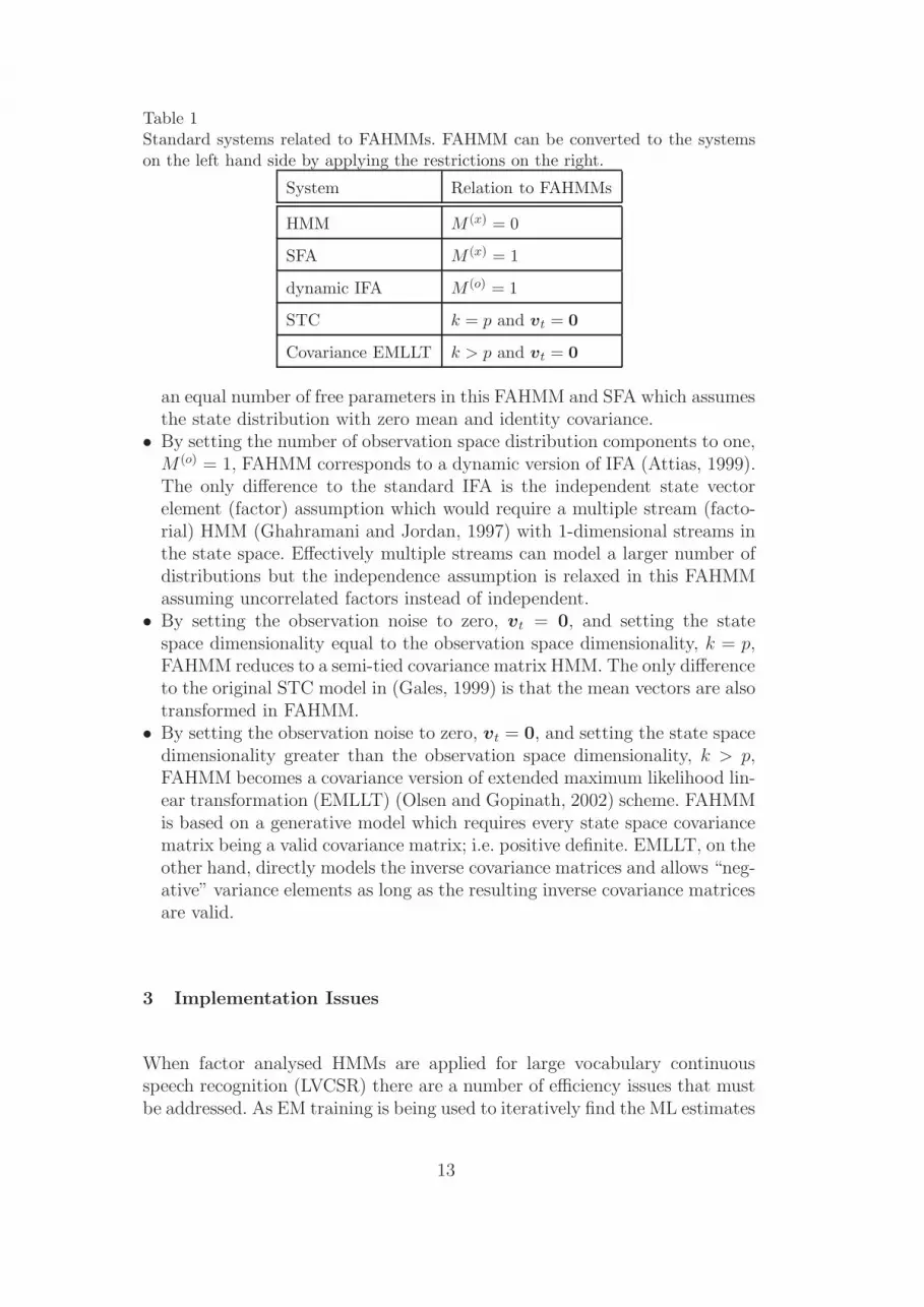
Table 1Standard systems related to FAHMMs. FAHMM can be converted to the systemson the left hand side by applying the restrictions on the right.

System Relation to FAHMMs

HMM M (x) = 0

SFA M (x) = 1

dynamic IFA M (o) = 1

STC k = p and vt = 0

Covariance EMLLT k > p and vt = 0

an equal number of free parameters in this FAHMM and SFA which assumesthe state distribution with zero mean and identity covariance.

• By setting the number of observation space distribution components to one,M (o) = 1, FAHMM corresponds to a dynamic version of IFA (Attias, 1999).The only difference to the standard IFA is the independent state vectorelement (factor) assumption which would require a multiple stream (facto-rial) HMM (Ghahramani and Jordan, 1997) with 1-dimensional streams inthe state space. Effectively multiple streams can model a larger number ofdistributions but the independence assumption is relaxed in this FAHMMassuming uncorrelated factors instead of independent.

• By setting the observation noise to zero, vt = 0, and setting the statespace dimensionality equal to the observation space dimensionality, k = p,FAHMM reduces to a semi-tied covariance matrix HMM. The only differenceto the original STC model in (Gales, 1999) is that the mean vectors are alsotransformed in FAHMM.

• By setting the observation noise to zero, vt = 0, and setting the state spacedimensionality greater than the observation space dimensionality, k > p,FAHMM becomes a covariance version of extended maximum likelihood lin-ear transformation (EMLLT) (Olsen and Gopinath, 2002) scheme. FAHMMis based on a generative model which requires every state space covariancematrix being a valid covariance matrix; i.e. positive definite. EMLLT, on theother hand, directly models the inverse covariance matrices and allows “neg-ative” variance elements as long as the resulting inverse covariance matricesare valid.

3 Implementation Issues

When factor analysed HMMs are applied for large vocabulary continuousspeech recognition (LVCSR) there are a number of efficiency issues that mustbe addressed. As EM training is being used to iteratively find the ML estimates

13

of the model parameters, an appropriate initialisation scheme is essential. Fur-thermore, in common with standard LVCSR systems, parameter tying may beused extensively. In addition, there is a large amount of matrix operations thatneed to be computed. Issues with numerical accuracy have to be considered.Finally, as there are two sets of hidden variables in FAHMMs, an efficient twolevel training scheme is presented.

3.1 Initialisation

One major issue with the EM algorithm is that there may be a number oflocal maxima. An appropriate initialisation scheme may improve the chancesof finding a good solution. A sensible starting point is to use a standard HMM.A single Gaussian mixture component HMM can be converted to an equivalentFAHMM as follows

µ(x)j = µj[1:k]

Σ(x)j =

1

2Σj[1:k]

Cj = I

µ(o)j =

0

µj[k+1:p]

Σ(o)j =

12Σj[1:k] 0

0 Σj[k+1:p]

where µj[1:k] represent the first k elements of the mean vector and Σj[1:k] isthe upper left k by k submatrix of the covariance matrix associated with statej of the initial HMM.

The above initialisation scheme guarantees that the average log-likelihood ofthe training data after the following iteration is equal to the one obtained usingthe original HMM. The equivalent FAHMM system can also be obtained bysetting the observation matrices equal to zero and initialising the observationnoise as the HMM output distributions. However, the proposed method canbe used to give more weight on certain dimensions and should provide betterconvergence. Here it is assumed that the first k feature vector elements arethe most significant. In the experiments, the state space dimensionality waschosen to be k = 13 which corresponds to the static parameters in a standard39-dimensional feature vector. Alternative feature selection techniques such asFisher ratio can also be used within this initialisation scheme.

14

3.2 Parameter Sharing

As discussed in Section 2.1, the number of free parameters per FAHMM state,η, is the same as in a factor analysis model with Gaussian mixture distri-butions. Table 2 summarises the numbers of free parameters per HMM andFAHMM state discarding the mixture weights. The dimensionality of the statespace, k, and the number of observation noise components, M (o), have thelargest influence on the complexity of FAHMMs.

Table 2Number of free parameters per HMM and FAHMM state, η, using M (x) statespace components, M (o) observation noise components and no sharing of individualFAHMM parameters. Both diagonal covariance and full covariance matrix HMMsare shown.

System Free Parameters (η)

diagonal covariance HMM 2M (o)p

full covariance HMM M (o)p(p + 3)/2

FAHMM 2(M (x) − 1)k + pk + 2M (o)p

When context-dependent HMM systems are trained the selection of the modelset is often based on decision-tree clustering (Bahl, de Souza, Gopalkrishnan,Nahamoo, and Picheny, 1991). However, implementing decision-tree cluster-ing for FAHMMs is not as straightforward as for HMMs. The clustering basedon single mixture component HMM statistics is not optimal for HMMs (Nock,Gales, and Young, 1997). Since the FAHMMs can be viewed as full covariancematrix HMMs, decision-tree clustered single mixture component HMM modelsmay be considered as a sufficiently good starting point for FAHMM initialisa-tion. The initialisation of the context-dependent models can be done the sameway as using standard context-independent HMMs described in Section 3.1.

In addition to state clustering, it is sometimes useful to share some of theindividual FAHMM parameters. It is possible to tie any number of parametersbetween an arbitrary number of models at various levels of the model. Forexample, the observation matrix can be shared globally or between classesof discrete states as in semi-tied covariance HMMs (Gales, 1999). A globalobservation noise distribution could represent a stationary noise environmentcorrupting all the speech data. Implementing arbitrary tying schemes is closelyrelated to those used with standard HMM systems (Young et al., 2000). Thesufficient statistics required for the tied parameter are accumulated over theentire class sharing it before updating. If the mean vectors and the covariancematrices of the state space noise are tied on a different level, all the cross termsbetween the first-order accumulates and the updated mean vectors, µjn, haveto be used in the covariance matrix update formula. Equation (14), includingall the cross terms, can be written as

15

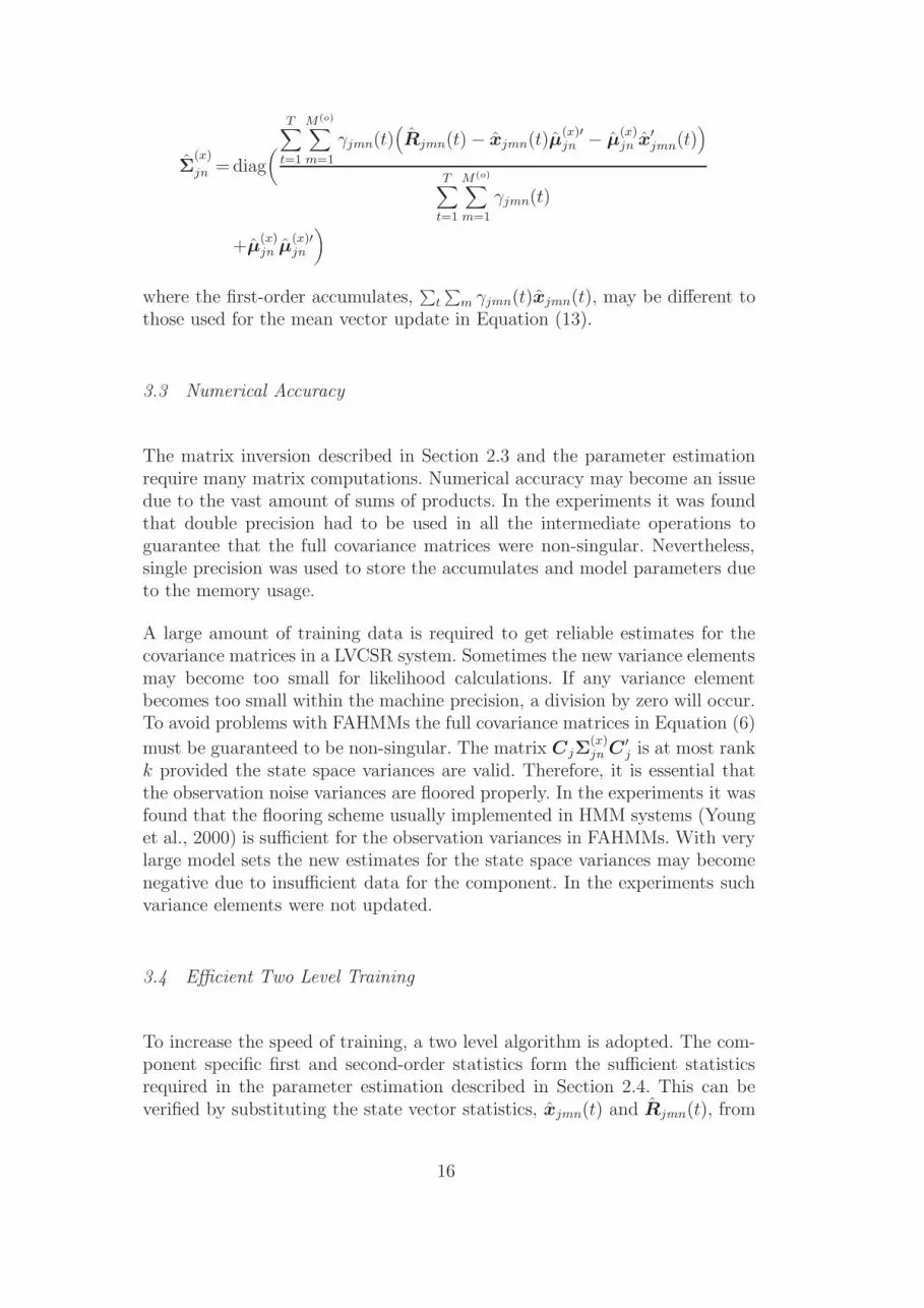
Σ(x)

jn = diag(

T∑

t=1

M (o)∑

m=1

γjmn(t)(

Rjmn(t) − xjmn(t)µ(x)′jn − µ

(x)jn x′

jmn(t))

T∑

t=1

M (o)∑

m=1

γjmn(t)

+µ(x)jn µ

(x)′jn

)

where the first-order accumulates,∑

t

∑

m γjmn(t)xjmn(t), may be different tothose used for the mean vector update in Equation (13).

3.3 Numerical Accuracy

The matrix inversion described in Section 2.3 and the parameter estimationrequire many matrix computations. Numerical accuracy may become an issuedue to the vast amount of sums of products. In the experiments it was foundthat double precision had to be used in all the intermediate operations toguarantee that the full covariance matrices were non-singular. Nevertheless,single precision was used to store the accumulates and model parameters dueto the memory usage.

A large amount of training data is required to get reliable estimates for thecovariance matrices in a LVCSR system. Sometimes the new variance elementsmay become too small for likelihood calculations. If any variance elementbecomes too small within the machine precision, a division by zero will occur.To avoid problems with FAHMMs the full covariance matrices in Equation (6)

must be guaranteed to be non-singular. The matrix CjΣ(x)jn C ′

j is at most rankk provided the state space variances are valid. Therefore, it is essential thatthe observation noise variances are floored properly. In the experiments it wasfound that the flooring scheme usually implemented in HMM systems (Younget al., 2000) is sufficient for the observation variances in FAHMMs. With verylarge model sets the new estimates for the state space variances may becomenegative due to insufficient data for the component. In the experiments suchvariance elements were not updated.

3.4 Efficient Two Level Training

To increase the speed of training, a two level algorithm is adopted. The com-ponent specific first and second-order statistics form the sufficient statisticsrequired in the parameter estimation described in Section 2.4. This can beverified by substituting the state vector statistics, xjmn(t) and Rjmn(t), from

16

Equations (10) and (11) into the update Equations (12)-(15). The sufficientstatistics can be written as

γjmn =T

∑

t=1

γjmn(t)

µjmn =T

∑

t=1

γjmn(t)ot

Rjmn =T

∑

t=1

γjmn(t)oto′t

Given these accumulates and the current model parameters, M, the requiredaccumulates for the new parameters can be estimated. Since the estimatedstate vector statistics depend on both the data accumulates and the currentmodel parameters an extra level of iterations can be introduced. After updat-ing the model parameters, new state vector distribution given the old dataaccumulates and the new model parameters can be estimated. These withiniterations are guaranteed to increase the log-likelihood of the data. Fig. 2 illus-trates the increase of the auxiliary function values during three full iterations,10 within iterations each.

2 4 6 8 10

−100

−95

−90

−85full iteration 1

no. within iterations

auxi

liary

func

tion

2 4 6 8 10

full iteration 2

no. within iterations2 4 6 8 10

full iteration 3

no. within iterations

Fig. 2. Auxiliary function values versus within iterations during 3 full iterations oftwo level FAHMM training.

The efficient training algorithm can be summarised as follows

(1) Collect the data statistics using forward-backward algorithm;(2) Estimate the state vector distribution p(xt|j, m, n, O,M);(3) Estimate new model parameters M;(4) If the auxiliary function value has not converged go to step 2 and update

the parameters M → M;(5) If the average log-likelihood of the data has not converged go to step 1

and update the parameters M → M.

The within iterations decrease the number of full iterations needed in training.The overall training time becomes shorter because less time has to be spentcollecting the data accumulates. The average log-likelihoods of the training

17

data against the number of full iterations are illustrated in Fig. 3. Four it-erations of embedded training were first applied to the baseline HMM. TheFAHMM system with k = 13 was initialised as described in Section 3.1. Both,one level training and more efficient two level training with 10 within itera-tions, were used and the corresponding log-likelihoods are shown in the figure.

0 2 4 6 8 10 12−76

−74

−72

−70

−68

−66

−64

−62

aver

age

log−

likel

ihoo

d

no. iterations

HMM baseline FAHMM one level training FAHMM two level training, 10 within iter

Fig. 3. Log-likelihood values against full iterations for baseline HMM and an untiedFAHMM with k = 13. One level training and more efficient two level training with10 within iterations were used.

4 Results

The results in this section are presented to illustrate the performance of someFAHMM configurations on medium to large speech recognition tasks. Onlya small number of possible configurations have been examined and the con-figurations have not been chosen in accordance with any optimal criterion.Generally, configurations with fewer or equivalent number of free parameterscompared to the baseline were chosen. The state space size, k = 13, was usedsince it was the number of static components in the chosen parameterisation.The aim was to show how FAHMMs perform with some possible configurationsas well as compare them to standard semi-tied systems.

18

4.1 Resource Management

For initial experiments, a standard medium size speech recognition task, theARPA Resource Management (RM) task, was used. Following the HTK “RMRecipe” (Young et al., 2000), the baseline system was trained starting froma flat start single Gaussian mixture component monophone system. A totalof 3990 sentences {train, dev aug} were used for training. After four itera-tions of embedded training, the monophone models were cloned to produce asingle mixture component triphone system. Cross word triphone models thatignore the word boundaries in the context were used. These initial triphonemodels were trained with two iterations of embedded training after which adecision-tree clustering was applied to produce a tied state triphone system.This system was used as an initial model set for standard HMM, STC andFAHMM systems. A total of 1200 sentences {feb89, oct89, feb91, sep92}with a simple word-pair grammar were used for evaluation.

The baseline HMM system was produced by standard iterative mixture split-ting (Young et al., 2000) using four iterations of embedded training per mix-ture configuration until no decrease in the word error rate was observed. Theword error rates with the number of free parameters per HMM state up to 6components are presented on the first row in Table 3, marked HMM. The bestperformance was 3.76% obtained with 10 mixture components. The numberof free parameters per HMM state in the best baseline system was η = 780per state. As an additional baseline a global semi-tied HMM system was built.The single mixture baseline HMM system was converted to the STC systemby adding a global full 39 by 39 identity transformation matrix. The numberof free parameters of the system increased by 1521 compared to the baselineHMM system. Since the number of physical states in the system was about1600, the number of model parameters per state, η, increased by less thanone. As discussed in Section 2.5, this STC system corresponds to a FAHMMwith state space dimensionality k = 39 and observation noise equal to zero.The number of mixture components was increased by the mixture splittingprocedure. Nine full iterations of embedded training were used with 20 withiniterations and 20 row by row transform iterations (Gales, 1999). The resultsare presented on the second row in Table 3, marked STC. The best semi-tied performance was 3.83% obtained with 5 mixture components. As usual,the performance when using STC is better with fewer mixture components.However, increasing the number of mixture components in a standard HMMsystem can be seen to model the intra-frame correlation better.

A FAHMM system with state space dimensionality k = 39 and a global obser-vation matrix, denoted as GFAHMM, was built for comparison with the STCsystem above. The global full 39 by 39 observation matrix was initialised to anidentity matrix and the variance elements of the single mixture baseline HMM

19

Table 3Word error rates (%) and number of free parameters, η, on the RM task, versus num-ber of mixture components for the observation pdfs, for HMM, STC and GFAHMMsystems.

System M (o) 1 2 3 4 5 6

HMMη 78 156 234 312 390 468

wer[%] 7.79 6.68 5.05 4.32 4.09 3.99

STCη 78 156 234 312 390 468

wer[%] 7.06 5.30 4.32 3.93 3.83 3.85

GFAHMMη 117 195 273 351 429 507

wer[%] 6.52 4.88 4.28 3.94 3.68 3.77

system were evenly distributed between the observation and state space vari-ances as discussed in Section 3.1. The number of state space components wasset to one, M (x) = 1, and the observation space components were increasedby the mixture splitting procedure. The system corresponds to a global fullloading matrix SFA with non-identity state space covariance matrices. Thenumber of additional free parameters per state was 39 due to the state spacecovariance matrices, which could not be subsumed into the global observationmatrix, and 1521 globally due to the observation matrix. Nine full iterationsof embedded training were used, each with 20 within iterations. The resultsare presented on the third row in Table 3, marked GFAHMM. The best per-formance, 3.68%, was achieved with 5 mixture components. The difference inthe number of free parameters between the best baseline, M (o) = 10, and thebest GFAHMM system, M (o) = 5, was 351 per state. Compared to the STCsystem, GFAHMM has only 39 additional free parameters per state. However,the GFAHMM system provides a relative word error rate reduction of 4% tothe STC system.

These initial experiments show the relationship between FAHMMs and STCin practise. However, the training and recognition using full state space FAH-MMs is far more complex than using global STC even though the observationmatrix is shared globally. Since STC does not have observation noise, theglobal transform can be applied to the feature vectors in advance and fullcovariance matrices are not needed in the likelihood calculation. It should benoted that the errors the above three systems make are very similar. Thiswas investigated by scoring the results of the systems against each other. Thehighest error rates for this cross evaluation were less than 2.50%. The per-formance of FAHMMs using lower dimensional state space is reported in theexperiments below.

20

4.2 Minitrain

The Minitrain 1998 Hub5 HTK system (Hain, Woodland, Niesler, and Whit-taker, 1999) was used as a larger speech recognition task. The baseline was adecision-tree clustered tied state triphone HMM system. Vocal tract lengthnormalisation (VTLN) was used to make the system gender independent.Cross word triphone models with GMMs were used. The 18 hour Minitrainset defined by BBN (Miller and McDonough, 1997) containing 398 conversa-tion sides of Switchboard-1 corpus was used as the acoustic training data. Thetest data set was the subset of the 1997 Hub5 evaluation set used in (Hainet al., 1999). The best performance, 51.0%, was achieved with 12 componentswhich corresponds to η = 936 parameters per state. The mixture splittingwas not continued further since the performance started degrading after 12components.

A FAHMM system with state space dimensionality 13 was built starting fromthe single mixture component baseline system. An individual 39 by 13 obser-vation matrix initialised as an identity matrix was attached to each state. Thefirst 13 variance elements of the HMM models were evenly distributed amongthe observation and state space variances as discussed in Section 3.1. The mix-ture splitting was started from the single mixture component baseline systemincreasing the number of state space components while fixing the number ofobservation space components to M (o) = 1. The number of observation spacecomponents of a single state space component system, M (x) = 1, was then in-creased and fixed to M (o) = 2. The number of the state space components wasincreased until no further gain was achieved and so on. The results up to thebest performance per column are presented in Table 4. As discussed in Section2.5, the row corresponding to M (x) = 1 is related to a SFA system and the firstcolumn corresponding to M (o) = 1 is related to a dynamic IFA without theindependent state vector element assumption. The same performance as thebest baseline HMM system was achieved using FAHMMs with 2 observationand 4 state space components, 51.0% (η = 741). The difference in the num-ber of free parameters per state is considerable: the FAHMM system has 195less than the HMM one. The best FAHMM performance, 50.7% (η = 793),was also achieved using fewer free parameters than the best baseline system,though the improvement is not statistically significant.

These experiments show how the FAHMM system performs in a large speechrecognition task when a low dimensional state space was used. As the statespace dimensionality and the initialisation were selected based on intuition,the results seem promising. Choosing the state space dimensionality auto-matically is very challenging problem, and it can be expected to improve theperformance. Complexity control and more elaborate initialisation schemeswill be studied in the future.

21

Table 4Word error rates (%) and number of free parameters, η, on the Minitrain task,versus number of mixture components for the observation and state space pdfs, forFAHMM system with k = 13. The best baseline HMM word error rate was 51.0%with M (o) = 12 (η = 936).

M (o) 1 2 4M (x)

1η 585 663 819

wer[%] 53.3 51.7 51.0

2η 611 689 845

wer[%] 53.3 51.4 51.3

4η 663 741 897

wer[%] 53.0 51.0 50.9

6η 715 793 949

wer[%] 52.8 50.7 51.0

8η 767 845

wer[%] 52.6 51.0

4.3 Switchboard 68 Hours

For the experiments performed in this section, a 68 hour subset of the Switch-board (Hub5) acoustic training data set was used. 862 sides of the Switchboard-1 and 92 sides of the Call Home English were used. The set is described as“h5train00sub” in (Hain, Woodland, Evermann, and Povey, 2000). As withMinitrain, the baseline was a decision-tree clustered tied state triphone HMMsystem with VTLN, cross word models and GMMs. The 1998 Switchboardevaluation data set was used for testing. The baseline HMM system worderror rates with the number of free parameters per state are presented onthe first row in Table 5, marked HMM. The word error rate of the baselinesystem went down to 45.7% with 30 mixture components. However, the num-ber of free parameters in such a system is huge, η = 2340 per state. The 14component system was a reasonable compromise because the word error rate,46.5%, seems to be a local stationary point. As an additional baseline a globalsemi-tied covariance HMM system was trained the same way as in the RMexperiments. The results for the STC system are presented on the second rowin Table 5, marked STC. The best performance, 45.7%, in the STC systemwas obtained using 16 components.

FAHMM system with state space dimensionality k = 13 was built startingfrom the single mixture component baseline system. The initialisation and

22

mixture splitting were carried out the same way as in the Minitrain experi-ments in Section 4.2. Unfortunately, filling up a complete table was not feasiblesince the training time grows very long. The number of full covariance matri-ces defined in Section 2.3 is M (o)M (x), and the memory is quickly filled whenusing effectively more than 16 full covariance matrices stored prior to trainingor recognition. Despite the efficient inversion and caching described in Section2.3, the training and recognition times grow too long with the current imple-mentation. The most interesting results here are achieved using only one statespace component which corresponds to the SFA. The results are presented onthe third row in Table 5, marked SFA. Increasing the number of state spacecomponents with a single observation space component, M (o) = 1, (IFA) didnot show much gains. This is probably due to the small increase in the num-ber of model parameters in such a system. It is worth noting that the bestbaseline performance was achieved using FAHMMs with considerably fewerfree parameters. The 12 component baseline performance, 46.7% (η = 936),was achieved by using FAHMMs with fewer parameters - namely M (o) = 2and M (x) = 8 which corresponds to η = 845 free parameters per state.

Table 5Word error rates (%) and number of free parameters, η, on the Hub5 68 hour task,versus number of mixture components for the observation pdfs, for HMM, STC,SFA and GSFA systems with k = 13. SFA is a FAHMM with a single state spacemixture component, M (x) = 1. SFA has state specific observation matrices whereasSTC and GSFA have global ones.

System M (o) 1 2 4 6 8 10 12 14 16

HMMη 78 156 312 468 624 780 936 1092 1248

wer[%] 55.1 52.4 49.6 48.5 47.7 47.2 46.7 46.5 46.5

STCη 78 156 312 468 624 780 936 1092 1248

wer[%] 54.3 50.4 48.4 47.3 46.7 46.3 46.3 45.8 45.7

SFAη 585 663 819 975 1131 1287 1443 1599 1755

wer[%] 49.1 48.0 47.2 46.6 46.3 46.4 46.0 45.8 45.9

GSFAη 91 169 325 481 637 793 949 1105 1261

wer[%] 55.2 52.1 49.4 48.4 47.4 46.9 46.7 46.4 46.1

To see how the tying of parameters influence the results, a FAHMM systemwith state space dimensionality k = 13 and a global observation matrix C wasbuilt starting from the single mixture component baseline system as usual.The initialisation was carried out the same way as in the Minitrain experi-ments in Section 4.2. As before, filling up the table was not feasible due to thenumber of effective full covariance components in the system. Examining thepreliminary results, the single state space component system appeared to bethe most interesting. The results for the single state space component system

23

are presented on the fourth row in Table 5, marked GSFA. The 12 observa-tion component system achieved the same performance as the 12 componentbaseline system but further increasing the number of components proved tobe quite interesting. The 16 observation space component system achieved46.1% (η = 1261), the same performance as 24 component baseline systembut with 611 free parameters fewer. It should also be noted that the STCsystem outperforms these configurations of FAHMMs in this task.

These experiments show that the current implementation of the FAHMM sys-tem has its limits when the task size is increased from the Minitrain task.The initialisation and choice of state space dimensionality require further at-tention, as previously indicated. The main contribution of these experimentswas to show how an equivalent performance to HMMs can be achieved usingdramatically fewer model parameters in a large speech recognition task withsimple configurations of FAHMMs.

5 Conclusions

This paper has introduced the factor analysed HMM which is a general formof acoustic model. It combines a standard Gaussian mixture HMM with ashared and independent factor analysis model. FAHMM should provide abetter model for the correlation between the feature vector elements com-pared to a standard diagonal covariance matrix HMM. It can be viewed asa compromise between diagonal and full covariance matrix systems. In addi-tion, FAHMM can be viewed as a general state space model which allows anumber of subspaces to be explored. A variety of configurations and sharingschemes, some of which correspond to standard systems, have been investi-gated. The ML estimation using EM algorithm is presented along with severalschemes to improve both, time and memory efficiency. The speech recogni-tion performance is evaluated in experiments using three medium to largevocabulary continuous speech recognition tasks. The results show that equiv-alent or slightly better performance compared to standard diagonal covarianceGaussian mixture HMMs can be achieved with considerably fewer model pa-rameters. The FAHMM with 2 observation and 8 state space components gaveperformance equal to the best HMM systems for both Minitrain and Hub5 68hour tasks.

Due to the flexibility of FAHMMs a large number of configurations can beexplored. The number of Gaussian mixture components in both, the state andobservation space, can be chosen. Different techniques to optimally choose theconfiguration have to be investigated. Another important question is how tochoose an optimal state space dimensionality. These are standard problems inspeech recognition and machine learning. The automatic complexity control

24

for FAHMM based systems has to be addressed in the future.

Acknowledgements

A-V.I. Rosti is funded by an EPSRC studentship and Tampere GraduateSchool in Information Science and Engineering. He received additional supportfrom the Finnish Cultural Foundation. This work made use of equipmentkindly supplied by IBM under an SUR award.

References

Attias, H., 1999. Independent factor analysis. Neural Computation 11 (4),803–851.

Bahl, L., de Souza, P., Gopalkrishnan, P., Nahamoo, D., Picheny, M., 1991.Context dependent modelling of phones in continuous speech using decisiontrees. In: Proceedings DARPA Speech and Natural Language ProcessingWorkshop. pp. 264–270.

Chen, S., Gopalakrishnan, P., 1998. Clustering via the Bayesian informationcriterion with applications in speech recognition. In: Proceedings Interna-tional Conference on Acoustics, Speech and Signal Processing. Vol. 2. pp.645–648.

Gales, M., 1998. Maximum likelihood linear transformations for HMM-basedspeech recognition. Computer Speech and Language 12 (2), 75–98.

Gales, M., 1999. Semi-tied covariance matrices for hidden Markov models.IEEE Transactions on Speech and Audio Processing 7 (3), 272–281.

Gales, M., 2002. Maximum likelihood multiple subspace projections for hiddenMarkov models. IEEE Transactions on Speech and Audio Processing 10 (2),37–47.

Ghahramani, Z., 1998. Learning dynamic Bayesian networks. In: Giles, C.,Gori, M. (Eds.), Adaptive Processing of Sequences and Data Structures.Vol. 1387 of Lecture Notes in Computer Science. Springer, pp. 168–197.

Ghahramani, Z., Jordan, M., 1997. Factorial hidden Markov models. MachineLearning 29 (2-3), 245–273.

Gopinath, R., Ramabhadran, B., Dharanipragada, S., 1998. Factor analysisinvariant to linear transformations of data. In: Proceedings InternationalConference on Speech and Language Processing. pp. 397–400.

Hain, T., Woodland, P., Evermann, G., Povey, D., 2000. The CU-HTK March2000 HUB5E transcription system. In: Proceedings Speech TranscriptionWorkshop.

Hain, T., Woodland, P., Niesler, T., Whittaker, E., 1999. The 1998 HTKsystem for transcription of conversational telephone speech. In: Proceedings

25

International Conference on Acoustics, Speech and Signal Processing. Vol. 1.pp. 57–60.

Harville, D., 1997. Matrix Algebra from a Statistician’s Perspective. Springer.Kumar, N., 1997. Investigation of silicon-auditory models and generalization

of linear discriminant analysis for improved speech recognition. Ph.D. thesis,Johns Hopkins University.

Liu, X., Gales, M., Woodland, P., 2003. Automatic complexity control forHLDA systems. In: Proceedings International Conference on Acoustics,Speech and Signal Processing. Vol. 1. pp. 132–135.

Miller, D., McDonough, J., May 1997. BBN 1997 Acoustic Modelling, pre-sented at Conversational Speech Recognition Workshop DARPA Hub-5EEvaluation.

Nock, H., Gales, M., Young, S., 1997. A comparative study of methods for pho-netic decision-tree state clustering. In: Proceedings European Conference onSpeech Communication and Technology. pp. 111–114.

Olsen, P., Gopinath, R., 2002. Modeling inverse covariance matrices by basisexpansion. In: Proceedings International Conference on Acoustics, Speech,and Signal Processing. Vol. 1. pp. 945–948.

Rosti, A.-V., Gales, M., 2001. Generalised linear Gaussian mod-els. Tech. Rep. CUED/F-INFENG/TR.420, Cambridge Univer-sity Engineering Department, available via anonymous ftp fromftp://svr-ftp.eng.cam.ac.uk/pub/reports/rosti_tr420.ps.gz.

Roweis, S., Ghahramani, Z., 1999. A unifying review of linear Gaussian models.Neural Computation 11 (2), 305–345.

Saul, L., Rahim, M., 1999. Maximum likelihood and minimum classificationerror factor analysis for automatic speech recognition. IEEE Transactionson Speech and Audio Processing 8 (2), 115–125.

Viterbi, A., 1967. Error bounds for convolutional codes and an asymptoticallyoptimal decoding algorithm. IEEE Transactions on Information Theory IT-13, 260–269.

Young, S., Kershaw, D., Odell, J., Ollason, D., Valtchev, V., Woodland, P.,2000. The HTK Book (for HTK Version 3.0). Cambridge University.

26