This content has been downloaded from IOPscience. Please scroll down to see the full text.

Download details:

IP Address: 94.198.34.230

This content was downloaded on 01/11/2013 at 06:34

Please note that terms and conditions apply.

Factorization of numbers with Gauss sums: I. Mathematical background

View the table of contents for this issue, or go to the journal homepage for more

2011 New J. Phys. 13 103007

(http://iopscience.iop.org/1367-2630/13/10/103007)

Home Search Collections Journals About Contact us My IOPscience

T h e o p e n – a c c e s s j o u r n a l f o r p h y s i c s

New Journal of Physics

Factorization of numbers with Gauss sums:I. Mathematical background

S Wölk1,4, W Merkel1, W P Schleich1, I Sh Averbukh2

and B Girard3

1 Institut für Quantenphysik, Universität Ulm, Albert-Einstein-Allee 11,D-89081 Ulm, Germany2 Department of Chemical Physics, Weizmann Institute of Science,Rehovot 76100, Israel3 Laboratoire de Collisions, Agrégats, Réactivité, IRSAMC (Université deToulouse/UPS; CNRS) Toulouse, FranceE-mail: sabine.woelk@uni-ulm.de

New Journal of Physics 13 (2011) 103007 (37pp)Received 16 August 2011Published 7 October 2011Online at http://www.njp.org/doi:10.1088/1367-2630/13/10/103007

Abstract. We use the periodicity properties of generalized Gauss sums tofactor numbers. Moreover, we derive rules for finding the factors and illustratethis factorization scheme for various examples. This algorithm relies solely oninterference and scales exponentially.

4 Author to whom any correspondence should be addressed.

New Journal of Physics 13 (2011) 1030071367-2630/11/103007+37$33.00 © IOP Publishing Ltd and Deutsche Physikalische Gesellschaft

2

Contents

1. Introduction 21.1. Gauss sums in physics . . . . . . . . . . . . . . . . . . . . . . . . . . . . . . 31.2. Why factor numbers with Gauss sums? . . . . . . . . . . . . . . . . . . . . . . 41.3. Various classes of Gauss sums . . . . . . . . . . . . . . . . . . . . . . . . . . 41.4. Summary of experimental work . . . . . . . . . . . . . . . . . . . . . . . . . 51.5. Alternative proposals for Gauss sum factorization . . . . . . . . . . . . . . . . 71.6. Overview . . . . . . . . . . . . . . . . . . . . . . . . . . . . . . . . . . . . . 8

2. Continuous Gauss sum 82.1. A tool to factor numbers . . . . . . . . . . . . . . . . . . . . . . . . . . . . . 92.2. A new representation . . . . . . . . . . . . . . . . . . . . . . . . . . . . . . . 132.3. The location and origin of maxima . . . . . . . . . . . . . . . . . . . . . . . . 142.4. Condition for destructive interference . . . . . . . . . . . . . . . . . . . . . . 162.5. Factorization . . . . . . . . . . . . . . . . . . . . . . . . . . . . . . . . . . . 17

3. Discrete Gauss sum 183.1. New representation . . . . . . . . . . . . . . . . . . . . . . . . . . . . . . . . 193.2. Analytical expressions . . . . . . . . . . . . . . . . . . . . . . . . . . . . . . 203.3. Factorization . . . . . . . . . . . . . . . . . . . . . . . . . . . . . . . . . . . 22

4. Reciprocate Gauss sum 234.1. Gauss reciprocity relation . . . . . . . . . . . . . . . . . . . . . . . . . . . . . 234.2. Analytical expressions . . . . . . . . . . . . . . . . . . . . . . . . . . . . . . 244.3. Factorization . . . . . . . . . . . . . . . . . . . . . . . . . . . . . . . . . . . 26

5. Conclusions and discussion 27Acknowledgments 27Appendix A. Quantum algorithm for the phase of a Gauss sum 27Appendix B. Factorization with an N-slit interferometer 30Appendix C. Absolute value of a finite Gauss sum 34References 35

1. Introduction

‘Mathematics is the abstract key that turns the lock of the physical universe.’ This quote byJohn Polkinghorne expresses in a poetic way the fact that physics uses mathematics as a toolto make predictions about physical phenomena such as the motion of a particle, the outcomeof a measurement or the time evolution of a quantum state. However, there exist situationsin which the roles of the two disciplines are interchanged and physical phenomena allow usto obtain mathematical quantities. In the present series of papers [1], we follow this path ofemploying nature to evaluate mathematical functions. Here, we choose the special example ofGauss sums [2] and show that they are ideal for factoring numbers. At the same time we mustissue the caveat that in contrast to the Shor algorithm [3], the proposed Gauss sum factorizationalgorithm in its most elementary version scales only exponentially since it is based solely oninterference and does not involve entanglement. However, there are already indications [4, 5]

New Journal of Physics 13 (2011) 103007 (http://www.njp.org/)

3

that a combination of entanglement and Gauss sums can lead to a powerful tool to tacklequestions of factorization.

Recent years have seen an impressive number of experiments implementing Gausssums in physical systems to factor numbers. These systems range from nuclear magneticresonance (NMR) methods [6–8] via cold atoms [9] and Bose–Einstein condensates (BECs)[10, 11], tailored ultrashort laser pulses [12, 13] to classical light in a multi-path Michelsoninterferometer [14, 15]. Although these experiments have been motivated by earlier versionsof this series of papers made available before publication, they have focused exclusively on avery special type of Gauss sum, that is, the truncated Gauss sum, which is not at the center ofthe present work. Indeed, throughout this series we concentrate on three types of Gauss sums:the continuous, the discrete and the reciprocate Gauss sum. Moreover, we propose experimentalrealizations with the help of chirped laser pulses [16, 17] interacting with appropriate atoms.

We pursue two steps: (i) first we show that the mathematical properties of Gauss sums allowus to factor numbers and (ii) then we present three elementary quantum systems to implementour method using chirped laser pulses and multi-level atoms. To each step we devote an article.There is good reason to separate the individual articles. The work presented in the two articlesis a combination of quantum optics and number theory (for an introduction to number theory,see, e.g., [18]). In order to avoid overloading the quantum optical aspects of the problem withnumber-theoretical questions, we deal with the mathematical properties of Gauss sums in thisarticle and address the realizations in the second part.

1.1. Gauss sums in physics

Gauss sums [19, 20] manifest themselves in many phenomena in physics and come in a widevariety. They are similar to Fourier sums with the distinct difference that the summation indexappears in the phase in a quadratic rather than a linear way.

Real-valued Gaussians are familiar from statistical physics. The integral over a finiteextension of a Gaussian leads to a higher transcendental that is, the error function. When theintegration is not along the real axis but along one of the diagonals of complex space, we arrive atan integral giving rise to the Cornu spiral. This geometrical object determines [21] the intensitydistribution of light on a screen in the far field of an edge. It is also an essential building blockof the Feynman path integral [22, 23] and the method of stationary phase [24].

One modern application of integrals over quadratic phases in physics is chirped laserpulses. Here, the frequency of the light increases linearly in time, giving rise to a quadraticphase. The resulting excitation probability is determined [25] by the complex-valued errorfunction, which is closely related to the Cornu spiral. Indeed, the Cornu spiral was observedin real-time excitation of Rb atoms by chirped pulses [26].

A generalization of the Cornu spiral arises when we replace the integration over thecontinuous variable by a summation over a discrete parameter. In this case, the Cornu spiralturns into a Gauss sum.

Sums have properties that are dramatically different from their corresponding integrals.This feature stands out most clearly in the phenomena of revivals and fractional revivals[27, 28]. In the context of the Cornu spiral, the transition from the integral to the sum leadsto the curlicues [29, 30], that is, Cornu spirals in Cornu spirals. The origin of this self-similarityis discreteness. In the Gauss sum, the question of whether a parameter takes on integer, rationalor irrational values is crucial, whereas in the error function integral it does not matter. This

New Journal of Physics 13 (2011) 103007 (http://www.njp.org/)

4

feature will also be of importance in the context of the factorization of numbers, which is thetopic of the present series of papers.

Gauss sums are at the very heart of the Talbot effect [31] that describes the intensitydistribution of the light close to a diffraction grating. They are also crucial in the familiarproblem of the particle in the box and are the origin of the design of quantum carpets [32] and thecreation of superpositions of distinct phase states (see, e.g., [33]) by nonlinear evolution [34].Moreover, there is an interesting connection [20] to the Riemann zeta function, which isdetermined by the Mellin transform of the Jacobi theta function. For complex-valued rationalarguments the zeta function leads to Gauss sums.

1.2. Why factor numbers with Gauss sums?

It is the exponential increase of the dimension of Hilbert space together with entanglement,that makes the quantum computer so efficient and ideal for the problem of factoring. Twolandmark experiments [35, 36] have implemented the Shor algorithm. They were based on eitherNMR [35] or optical [36] techniques, and they were able to factor the number 15.

Our proposal outlined in this series of papers follows a different approach. It aims for ananalogue computer that relies solely on interference [37] without using entanglement. We test ifa given integer ` is a factor of the integer N , to be factored. Since we have to try out at least

√N

such factors, the method scales exponentially with the number of digits of N . It is therefore aclassical algorithm. This fact is not surprising since our method does not take advantage of theexponential resources of the Hilbert space.

At the heart of the Shor algorithm is the task of finding the period of a function [38]. Inour approach, we also use properties of a periodic function. It is the periodicity of the Gausssum that allows us to factor numbers. For this purpose, we construct a system whose output is aGauss sum. In this sense, nature is performing the calculation for us.

But why are Gauss sums ideal tools for the problem of factorization? Gauss sums play animportant role in number theory as well as physics. Three examples may testify to this claim:(i) the distribution of prime numbers is determined by the nontrivial zeros of the Riemann zetafunction, which is related [20] to the Gauss sums, (ii) a quantum algorithm [39–41] allows usto calculate the phase of a Gauss sum efficiently, and (iii) the Gauss reciprocity law can beinterpreted [42] as the analogue of the commutation relation between position and momentumoperators in quantum mechanics.

1.3. Various classes of Gauss sums

In order to lay the groundwork for part II of this series, we devote this paper to an overviewof the mathematical properties of several Gauss sums, that arise in different physical systems.When we study the two-photon excitation through an equidistant ladder system with a chirpedlaser pulse, we arrive [25] at the sum

SN (ξ)∼

∑m

wm exp

[2π i

(m +

m2

N

)ξ

]. (1)

Here N is expressed in terms of parameters characterizing the harmonic manifold and theargument ξ is proportional to the rescaled chirp of the laser pulse. The distribution of weightfactors wm is governed by the shape of the laser pulse. The sum SN contains linear as well asquadratic phases.

New Journal of Physics 13 (2011) 103007 (http://www.njp.org/)

5

Table 1. Summary of characteristic features of experiments factoring numbersusing Gauss sums. All experiments are based on the Gauss sum A(M)N (`) definedby (4) or closely related ones. Here we list the system, the number of digits of thenumber N to be factored, the number of terms M in the sum and some importantfeatures associated with the specific approach.

System N (digits) M

NMR [6–8] 17 10 Higher-ordertruncated Gauss sum,random terms

Cold atoms [9] 6 15 A large number ofpulses

BEC [10, 11] 5 10 Enhanced visibilityUltra-short laser pulses [12, 13] 13 30 Random termsA multi-path Michelson interferometer [14, 15] 6 3 N , ` are varied independently

Quite different sums emerge for a one-photon transition in a two-level atom interactingwith two driving fields. Here, we find two different types of Gauss sums depending on thetemporal shape of the fields. For a sinusoidal modulation of the excited state and a weak-drivingfield, the corresponding excitation probability amplitude is proportional to the sum

SN (`)∼

∑m

wm exp

[2π i m2 `

N

], (2)

which depends on purely quadratic phases.In the second realization, the modulating field causes a linear variation of the excited state

energy and the one-photon transition is driven by a train of equidistant delta-shaped laser pulses.The excitation probability amplitude is proportional to the sum

AN (`)∼

∑m

exp

[−2π i m2 N

`

](3)

at integer arguments `, which is again of the form of a Gauss sum. In comparison to SN (`), nowthe roles of the argument ` and the number N to be factored are interchanged.

1.4. Summary of experimental work

Several experiments [6–15] have already successfully demonstrated factorization with the helpof Gauss sums. We now briefly summarize them and we highlight important features in table 1.

The first set of experiments relies on the interaction of a sequence of electromagneticpulses with a two-level quantum system. The phase of each pulse is adjusted such that thetotal excitation probability is determined by a Gauss sum [6, 43]. Two realizations of two-level systems have been pursued: in NMR experiments [6–8], the two levels correspond tothe two orientations of the spin, for example the proton of the water molecule. However, also,optical pumping in laser-cooled atoms creates [9] an effective two-level situation, for examplethe hyperfine states of rubidium.

New Journal of Physics 13 (2011) 103007 (http://www.njp.org/)

6

The second type of experiments utilizes a sequence of appropriately designed femtosecondlaser pulses [12, 13]. The intensity at a given frequency component of this light is given by theinterference of this component of the individual pulses giving rise to a sum. With the help of apulse shaper it is possible to imprint the phases necessary for obtaining a Gauss sum determiningthe light intensity at a given frequency.

The third class of experiments [14, 15] is based on a multi-path Michelson inter-ferometer [44]. Here the phase shifts accumulated in the individual arms increase quadraticallywith arm length. This experiment does not suffer from the problem [45] that the ratio N/` hasto be precalculated. Moreover, they calculate the truncated Gauss sum not only for integer trialfactors ` but also for rational arguments ξ = q/r . Gauss sums at rational arguments open up anew avenue towards factorization [46].

The experiment reported in [10, 11] plays a very special role in this gallery of factorizationexperiments using Gauss sums: (i) it is the only one so far that has used a BEC, (ii) thereadout utilizes the momentum distribution and (iii) it relies on a generalization of Gausssums. Furthermore, they claim better visibility by using the probability distribution for highermomenta.

All of these studies have implemented the Gauss sum

A(M)N (`)≡1

M + 1

M∑m=0

exp

(−2π i m2 N

`

), (4)

which is closely related to the ones discussed in this paper. Here M + 1 is the number ofinterfering paths, which could be the number of laser pulses, or the number of arms in theMichelson interferometer.

With this type of Gauss sum, the idea of factorization is straightforward: when ` is a factorof N , N/` is an integer. As a result, the phase of each term in the Gauss sum A(M)N (`) is aninteger multiple of 2π , and due to constructive interference, the value of the sum is unity. Fora non-factor ` the ratio N/` is a rational number, and due to the quadratic variation of thephase, the individual terms interfere destructively. This feature leads to the unique criterionfor distinguishing factors from non-factors: for factors the sum A(M)N (`) is unity, whereas fornon-factors it is not.

However, a closer analysis [47] reveals the fact that for a subset of test factors, which arenot factors, the Gauss sum A(M)N (`) takes on values rather close to unity. It is therefore difficultto distinguish them from the real factors. These test factors have been called ghost factors. Thenumber of ghost factors increases as the number N to be factored increases.

Two techniques to suppress ghost factors offer themselves: (i) a Monte-Carlo evaluation[8, 13] of the complete Gauss sum

A(`−1)N (`)≡

1

`

`−1∑m=0

exp

(−2π i m2 N

`

)(5)

and (ii) the use [48] of exponential sums

A( j,M)N (`)≡

1

M + 1

M∑m=0

exp

(−2π i m j N

`

)(6)

with 16 j .

New Journal of Physics 13 (2011) 103007 (http://www.njp.org/)

7

Ghost factors originate from the fact that the phase of consecutive terms in a Gauss sumsuch as in (4) can increase very slowly. To take terms of A(M)N randomly allows the Gauss sumto interfere destructively rather rapidly. This technique has been demonstrated in experimentswith femtosecond pulses [13] and a 13-digit number could be factored with a very few pulses.Also an NMR experiment [8] followed this approach and factored a 17-digit number consistingof two prime numbers.

It is interesting to note that the argument for the factorization with the Gauss sum A(M)N (`)

does not make use of the fact that the phase varies quadratically. It is correct for any phase ofthe form m j , where j is an integer. The advantage of powers larger than two is that in this casethe cancellation of neighboring terms is faster. This technique has been applied successfully inNMR experiments [8] for j = 5 and a 17-digit number could be factored.

1.5. Alternative proposals for Gauss sum factorization

It is interesting to compare and contrast the Gauss sums and our proposals for factoring numbersto other suggestions along these lines. Here, we refer especially to the pioneering algorithmoutlined in [49] based on the Talbot effect. This method uses the intensity distribution of lightin the near-field of an N -slit grating. The number N to be factored is encoded in the numberof slits of period d. For a fixed separation z of the screen from the grating, we now vary thewavelength λ of the light. The factors of N emerge for those wavelengths where all maxima ofthe intensity pattern are equal in height. In appendix B, we show that in this case the intensitydistribution follows from the Gauss sum:

G(ξ)≡

√1

l

N−1∑n=0

exp

[−2π i

[n

lξ −

n2

2l

]], (7)

where ξ ≡ x/d is the scaled position on the screen and l ≡ λz/d2 is the dimensionless Talbotdistance.

We emphasize that in contrast to the sum A(M)N defined by (4), the sum G given by (7)contains N rather than M + 1 terms. Moreover, N does not enter into the phase factors of G.

In [50], the idea of factorization with an N -slit interferometer [49] was translated into onewith a single Mach–Zehnder interferometer. Furthermore, the work [50] suggests a way to testseveral trial factors, by connecting several Mach–Zehnder interferometers.

Another proposal [51–54] is based on wave packet dynamics in anharmonic potentialsgiving rise to quadratic phase factors. Here, the factors of an appropriately encoded number Ncan be extracted from the autocorrelation function. This quantity is in the form of a Gauss sumand experimentally accessible.

This approach is closely related to ideas [55, 56] to use rotor-like systems with a quadraticenergy spectrum for quantum computing. Initially, the wave packet is localized in space. At therevival time Trev the packet is identical to the initial one. However, it is not the revivals but ratherthe fractional revivals, that are interesting in the context of factorization. At times t = Trev/N ,with N odd, the wave is localized at N equally spaced positions. If N is even, there exist onlyN/2 such positions. This phenomenon can be used to build a K -bit quantum computer [55, 56]with K ≈ log2 N . It can also be employed for factorization [57]. For times t = l/N , with N odd,there exist N maxima of the probability distribution if N and l are coprime. But if they share acommon factor p that is l = p · r and N = p · q, we can only observe q maxima.

New Journal of Physics 13 (2011) 103007 (http://www.njp.org/)

8

We conclude our discussion of alternative proposals for Gauss sum factorization bybriefly mentioning the idea [58] of using two Josephson phase qubits, that are coupled to asuperconducting resonator. Here, the time evolution generates a phase shift of φk = 2πk2 N/`.With the help of a quantum phase measurement, the Gauss sum can be calculated.

1.6. Overview

This paper is organized as follows. In section 2, we introduce the continuous Gauss sum anddemonstrate its potential to factor numbers using two examples. Moreover, a remarkable scalingrelation of this type of Gauss sum allows us to use the realization of the Gauss sum for thenumber N to obtain information on the factors of another number N ′. We then turn in section 3to an investigation of the properties of the continuous Gauss sum for integer arguments. Thisapproach connects the Gauss sums central to this paper to the standard Gauss sums discussed inthe mathematical literature. In this way, we establish rules on how to identify factors of a numberusing the continuous Gauss sum evaluated at integers. We devote section 4 to yet another type ofGauss sum and connect it to the continuous Gauss sum at integer values. Section 5 summarizesthe key results that are relevant for part II of this series of papers.

In order to make the paper self-contained, we have included several appendices. Inappendix A, we outline the quantum algorithm [39–41] for evaluating the phase of a specificclass of Gauss sums. In order to provide a comparison with the ideas proposed in this paper, wethen briefly summarize in appendix B the essential ingredients of the approach to factor numberswith an N -slit interferometer [49]. We conclude in appendix C by deriving the absolute valueof a specific finite Gauss sum that is central to the discussion of revivals, and the factorizationtechnique based on the continuous Gauss sum and the N -slit interferometer.

2. Continuous Gauss sum

In this section, we study the periodicity properties of the continuous Gauss sum

S(ξ ; A, B)≡

∞∑m=−∞

wm exp

[2π i

(m

A+

m2

B

)ξ

](8)

with respect to the possibility of factoring numbers. Here, A and B denote two real numbersand the argument ξ assumes real values. The weight factors wm are centered around m = 0 andare slowly varying as a function of m.

We establish three results: (i) when B/A is an integer we can use the continuous Gausssums S to factor numbers. (ii) Maxima of |S(ξ ; A, B)| located at an integer ξ allow us toidentify factors. (iii) By an appropriate scale transformation we can factor any number N usingthe Gauss sum corresponding to another number N ′.

In order to derive these results, we first motivate these properties of the Gauss sumand then derive a new representation. This function allows us to choose the parametersappropriate for this technique. Moreover, we show that it is also possible to factor evennumbers.

New Journal of Physics 13 (2011) 103007 (http://www.njp.org/)

9

ξ

N = 33

3 5 7 9 11 13

|S33(ξ)|2

4.8 5 5.2 12.8 13 13.2

2.8 3 3.2 10.8 11 11.2

Figure 1. Factorization of the odd number N = 33 = 3 × 11 with the help of thecontinuous Gauss sum |S33(ξ)|

2 given by (9). The insets magnify the behavior of|S33(ξ)|

2 in the immediate neighborhood of test factors. The pronounced maximaat the factors 3 and 11 are clearly visible in the insets at the bottom. In contrast,at non-factors the signal does not show any peculiarities as exemplified at the topby `= 5 and `= 13. The width of the Gaussian weight function, (10), is givenby 1m = 10 and the summation over m covers 2M + 1 = 81 terms.

2.1. A tool to factor numbers

We start our analysis of the continuous Gauss sum by considering the special case A = 1 andB = N , that is,

SN (ξ)≡

∞∑m=−∞

wm exp

[2π i

(m +

m2

N

)ξ

]. (9)

In figure 1, we show |SN (ξ)|2 for the example N = 33 = 3 × 11 and the Gaussian weight factors

wm ≡

√1

2π1m2exp

[−

1

2

( m

1m

)2]

(10)

of width 1m = 10.Our main interest is in the behavior of |SN (ξ)|

2 in the vicinity of candidate prime factorsξ = `. Indeed, the insets of figure 1 at the bottom bring out most clearly distinct maxima atvalues of ξ corresponding to the factors `= 3 and `= 11. At non-factors such as `= 5 or`= 13 illustrated by the insets on the top, the continuous Gauss sum S33 does not show anypeculiarities. This example suggests that the continuous Gauss sum SN represents a tool forfactorization.

New Journal of Physics 13 (2011) 103007 (http://www.njp.org/)

10

|S(ξ;1,33)|2

|S(ξ;8,33)|2

|S(ξ;33/7,33)|2

2.8 3.0 3.2ξ

A = 1

A = 8

A = 33/7

Figure 2. Role of the parameter A in the method of factoring a number withthe help of the continuous Gauss sum S(ξ ; A, B) defined by (8). We depict|S(ξ ; A, 33)|2 in the vicinity of the factor ξ = 3 for three different values ofA and note that for A = 1 (top) and A = 33/7 (bottom) the quantity |S|2 shows adistinct maximum at ξ = 3. However, for A = 8 (middle) it does not display anypeculiarities.

We now turn to the role of the parameter A in the continuous Gauss sum S. For thispurpose, we analyze in figure 2 the function |S(ξ ; A, B)|2 for the example B = 33 and differentarguments A = 1, 8 and 33/7 in the vicinity of the factor ξ = 3 of N = B = 33. For the caseA = 8 (middle), the distinct maxima at the factor ξ = 3 of N = 33 is not visible anymore. On theother hand, for A = 33/7 (bottom) the absolute value |S(ξ ; A, B)|2 shows the same behavioras SN (ξ). As a consequence, the continuous Gauss sum S(ξ ; A, B) allows factorization only ifB/A is an integer number.

New Journal of Physics 13 (2011) 103007 (http://www.njp.org/)

11

9 10.2 11

|S51(ξ)|

6C 7C 8C

=ξ = 10.2 = 7C

=

Figure 3. Scaling property of the continuous Gauss sum illustrated by theexample |S51(ξ)|. The dominant maximum at ξ = 10.2 does not correspond toa factor of N = 51 because 10.2 is not an integer. However, by rescaling thehorizontal axis, that is, the variable ξ with the help of a new unit C, we canidentify this maximum as the factor of a different number N ′. Indeed, the choiceξ = 10.2 ≡ 7C with C ≡ 51/35 yields the factor 7 of N ′

≡ N/C = B/C = 35.The lower axis indicates this new scaling.

Furthermore, figure 1 displays maxima at non-integer values of ξ as well. For example, wefind that |S51(ξ)| shows a maximum at ξ = 10.2 as indicated by figure 3. Because ξ = 10.2 is anon-integer, it is thus not relevant in the context of factoring the number N = 51. However, byrescaling the argument ξ with

ξ ≡ ξ ′· C (11)

and C = 51/35, we find that this maximum corresponds to the integer number ξ ′= 7. This

feature is remarkable, because ξ ′= 7 is a factor of N ′

≡ 51/C = 35. As a consequence, thesignal |SN (ξ)| contains information not only about the factors of N but also about othernumbers N ′.

This scaling property of the Gauss sums suggests to store a master curve |SN (ξ)| on a cardsmall enough to be carried in the pocket, which can be used to factor any other number N ′, that isof the same order as N . For this reason, the scaling property of the Gauss sum and the associatedpossibility to factor many numbers have been jokingly called [59] ‘pocket factorizator’.

In figure 4, we illustrate the working principle of the pocket factorizator for N ′= 35

and N ′= 65 starting from the original signal associated with N = 51. Candidate prime factors

indicated on the left vertical axis are marked by horizontal lines. In order to find the adequatescale ξ ′ given by (11) for the number N ′, we adapt the slope of the tilted line appropriate forN ′. On the right vertical axis, we depict numbers N ′ < N and on the horizontal axis numbersN < N ′. In order to test whether the prime argument ` is a factor of N ′, we follow the horizontalline representing ` to the intersection with the tilted line. The ordinate ξ of the intersection point

New Journal of Physics 13 (2011) 103007 (http://www.njp.org/)

12

5155576569778595115

1

3

5

7

11

13

17

19

23

15

21

3335

39

3

5

17

5 13

7

155315

35

5656

Figure 4. The working principles of the pocket factorizator illustrated by thefactorization of the numbers N ′

= 35 and N ′= 65 using the Gauss sum SN for

N = 51. On the right vertical axis and the horizontal bottom axis, we showthe numbers N ′ to be factored in the domains N ′ < N = 51 and N ′ > N = 51,respectively. In order to factor the number N ′ using the master signal |S51(ξ)|

2

shown in the top row, we need to rescale the horizontal axis according tothe transformation ξ ′

≡ (N ′/N ) · ξ . We achieve this task nomographically byconnecting the left upper corner marking the origin of the master signal withthe point N ′ located either on the right vertical axis or the horizontal bottom axisby a straight line. We illustrate this procedure for the numbers N ′

= 35, N = 51and N ′

= 65 by dotted, solid and dashed lines, respectively. To test whether theprime argument ` is a factor of N ′, we follow the horizontal lines representingthe prime numbers marked on the left vertical axis to the intersection with thetilted line. The ordinate of the intersection point defines the relevant part of thesignal.The insets show the magnified signal in the neighborhood of the primefactors of N and N ′. A maximum of the signal at an integer identifies a factor asindicated by the insets for N ′

= 35 or N = 51 (top) and N ′= 65 (bottom).

New Journal of Physics 13 (2011) 103007 (http://www.njp.org/)

13

yields the section of the signal, that has to be analyzed. When the signal displays a maximumat an integer value of ξ ′, we have found a factor of N ′ as indicated by magnified insets of thesignal.

2.2. A new representation

In the preceding section, we have shown for specific choices of the parameters A and B that thecontinuous Gauss sum S(ξ ; A, B) allows us to factor numbers. In the following sections, wenow verify this property in a rigorous way.

For this purpose, we rewrite the sum, (8), in an exact way so as to bring out the features ofS = S(ξ ; A, B) typical of the different domains of ξ . Here, we concentrate on arguments

ξ ≡q

rB + δ (12)

that are close to a fraction q/r of B. We use a method that has been developed in the context offractional revivals of wave packets [27, 28].

When we substitute the representation (12) of ξ into the term of the Gauss sum, that isquadratic in m, we find

S =

∞∑m=−∞

wm exp[2π i

q

rm2

]exp

[2π i

(ξ

Am +

δ

Bm2

)]. (13)

Next, we recall the representation

∞∑m=−∞

am =

r−1∑p=0

∞∑n=−∞

ap+nr (14)

of one sum by a sum of sums which yields

S =

r−1∑p=0

∞∑n=−∞

wp+nr exp[2π i

q

r(p2 + 2pnr + n2r 2)

]exp

{2π i

[ξ

A(p + nr)+

δ

B(p + nr)2

]}(15)

or

S =

r−1∑p=0

exp[2π i

q

rp2

] ∞∑n=−∞

wp+nr exp

{2π i

[ξ

A(p + nr)+

δ

B(p + nr)2

]}. (16)

Here, we have made use of the identity

exp [2π is] = 1 (17)

for integer s.With the help of the Poisson summation formula

∞∑n=−∞

fn =

∞∑m=−∞

∫∞

−∞

dν f (ν)e−2π imν, (18)

New Journal of Physics 13 (2011) 103007 (http://www.njp.org/)

14

where f (ν) denotes the continuous extension of fn with f (n)≡ fn for integer values of ν, wearrive at

S =

r−1∑p=0

exp[2π i

q

rp2

] ∞∑m=−∞

∫∞

−∞

dν w(p + νr) exp

{2π i

[ξ

A(p + νr)+

δ

B(p + νr)2 − mν

]}.

(19)

Here, w(µ) denotes the continuous extension of wm with w(m)≡ wm .The substitution µ≡ p + νr finally leads us to

S =

∞∑m=−∞

1

r

r−1∑p=0

exp[2π i

(q

rp2 +

m

rp)]

(20)

×

∫∞

−∞

dµ w(µ) exp

[2π i

(ξ

A−

m

r

)µ

]exp

[2π i

δ

Bµ2

], (21)

where we have also interchanged the summations over m and p.As a consequence, we can represent S(ξ ; A, B) in the form

S(ξ ; A, B)=

∞∑m=−∞

W (r)m I

(r)m (ξ ; A, B) (22)

with the finite Gauss sum [2]

W (r)m ≡

1

r

r−1∑p=0

exp[2π i

(q

rp2 +

m

rp)]

(23)

and the shape functions

I(r)m (ξ ; A, B)≡

∫∞

−∞

dµ w(µ) exp

[2π i

(ξ

A−

m

r

)µ

]exp

[2π i

δ

Bµ2

]. (24)

2.3. The location and origin of maxima

According to (22) the continuous Gauss sum S in the neighborhood of ξ ∼= q B/r consists of asum of the products W (r)

m I(r)m of the finite Gauss sum W (r)m and the shape function I(r)m . Its role

stands out most clearly for the example of the continuous extension

w(µ)≡

√1

2π1m2exp

[−

1

2

( µ

1m

)2]

(25)

of the Gaussian weight function wm given by (10).In this case, we can perform the integral, (24), and find the complex-valued Gaussian

I(r)m =N exp

[−

(m − m

σ

)2

(1 + iDδ)

](26)

New Journal of Physics 13 (2011) 103007 (http://www.njp.org/)

15

of width

σ 2(δ)≡ σ 20 (1 + D2δ2) (27)

and centered around

m ≡ qB

A+

r

Aδ. (28)

Here, we have introduced the abbreviations

σ 20 ≡ σ 2(0)≡

r 2

2π 21m2(29)

for the width at δ = 0 as well as

D ≡ 4π1m2

B, (30)

together with the normalization constant

N ≡

√1

1 − i Dδ. (31)

It is the size of the width σ , that determines how many terms contribute to the sum overm in (22). Indeed, when σ < 1, that is, for a narrow Gaussian, only the m-value closest to mcontributes, whereas when 1< σ , that is, for a broad distribution, shape functions I(r)m of manyneighboring m-values have to be added up in order to yield S. In this case, the fact that I(r)m is acomplex-valued Gaussian with a quadratic phase variation as expressed by the last term in theexponential of (26) becomes important.

Indeed, we recall from appendix C that the absolute value |W (r)m | of the finite Gauss sum

is either constant as a function of m or oscillates between a constant and zero depending on rbeing odd or even. As a result all terms I(r)m contribute with equal weight or not at all. Althoughthe phases ofW (r)

m vary rapidly [32] with m, they cannot compensate for the quadratic variationin m of the phase factor governing the shape function I(r)m . As a result the sum over severalm-values leads to a destructive interference and a small value for S.

Figure 5 illustrates this single-maximum versus destructive interference-of-many-termsbehavior for the signal |S51(ξ)|

2 depicted in the inset. The dominant maximum at ξ =

(7/35)51 marked by a triangle arises solely from the term I(35)7 . On the other hand, for

ξ = (7/35)51 + 3/35, several terms I(35)m depicted by filled circles interfere destructively leading

to a suppression of the signal.Hence, the width σ of the Gaussian shape function (26) governs the value of S. According

to the definition (27) of σ , the smallest value of σ appears for δ = 0. Provided σ0 � 1 a singleterm in the sum, corresponding to the m-value m ′ closest to m, will contribute. In this case,the size of the shape function I(r)m′ is governed by exp[−(m ′

− m)2/σ 20 ]. Obviously, the largest

signal arises when m is an integer m0, since then the argument of the Gaussian I(r)m0vanishes.

According to the definition (28) of m, we find with δ = 0 for this optimal case the condition

m0 = qB

A, (32)

New Journal of Physics 13 (2011) 103007 (http://www.njp.org/)

16

0

1

1 7 10 20

0�5

|I(35)m|

m

|S51(ξ)|

ξ35735

36035

Figure 5. Dominant maxima versus small values of the continuous Gauss sum|SN (ξ)| identified with the help of the sum (22) as originating from a single-shape function I(r)m , or from the destructive interference of several of themillustrated for N = 51. The inset shows |S51(ξ)| as a function of ξ , which displaysa clear maximum at ξ = 357/35 = (7/35)51. Here, the deviation δ vanishesand therefore only the term I(35)

7 is relevant for the Gauss sum. On the otherhand, for ξ = 360/51 = (7/35)51 + 3/35, we find δ = 3/35. As a consequence,several shape functions I(35)

m interfere destructively in the sum (22), leading to asignificantly reduced signal.

which for q = 1 yields the condition that B/A must be an integer; otherwise we cannot obtaina maximum.

We conclude by noting that due to the definition (12) of ξ the condition δ = 0 for amaximum to occur translates into the value

ξ =q

rB, (33)

for the location. Hence, the maxima of the continuous Gauss sum S appear for integer multiplesof B/r . However, they only emerge provided σ0 � 1 and B/A is an integer.

2.4. Condition for destructive interference

In the previous section, we have identified the decisive role of the width σ0 in allowing fordominant maxima in S. In particular, we have established the necessary condition σ0 � 1 forthe occurrence of maxima. We now derive a criterion for the destructive interference of manyshape functions I(r)m in the sum (22).

This property arises from the condition

1 � σ(δ)= σ0(1 + D2δ2)1/2 (34)

on the width, which implies that[1

σ 20

− 1

]� D2δ2. (35)

New Journal of Physics 13 (2011) 103007 (http://www.njp.org/)

17

When we recall the constraint σ 20 � 1 necessary for the occurrence of a maximum which

implies that 1 � 1/σ 20 , we can neglect the term unity in the square and require the condition

1

σ 20

� D2δ2, (36)

which is even more general than the inequality (35).With the help of the definitions (29) and (30) of σ0 and D, we find that

1

r 2� 81m2

(δ

B

)2

. (37)

As a consequence, the width 1m2 depends on the minimal value of δ, that we want todiscriminate from zero. For factoring the number N , we estimate the continuous Gauss sumat arguments

ξ = `C (38)

with C = B/N . As a consequence, the parameter δ from (12) is given by

δ = ξ −q

rB = `

B

N−

q

rB =

` · r − q N

NrB, (39)

and therefore |δ| is larger than B/(Nr) if it is non-vanishing. As a result, the condition of (37)reduces to

1 � 81m2

N 2, (40)

which is independent of r .In summary, if 1m is larger than r and N , and B/A is integer, we can distinguish between

δ = 0 and δ 6= 0. In this case, we see peaks if and only if δ = 0, which will help us to factor thenumber N as demonstrated in the following section.

2.5. Factorization

We now show that the continuous Gauss sum S(ξ ; A, B) given by (8) and represented for aGaussian weight function wm defined by (10) by a sum of complex-valued Gaussians given by(22) offers a tool to factor numbers. Here, we distinguish between odd and even numbers to befactored. Needless to say, the last case is not of practical interest since we can always extractpowers of 2 from an even number. Nevertheless, it is interesting from a principle point of view.In particular, it brings out the crucial role of the finite Gauss sum W (r)

m in our factorizationscheme.

2.5.1. Odd numbers. In the examples discussed in section 2.1, we have found factors bysearching for maxima at arguments ξ which are integer multiples of C , that is, ξ = `C .In section 2.3, we have shown that maxima correspond to arguments ξ = (q/r)B. As aconsequence, the identity (12) transforms for maxima at ξ = `C into

` · C =q

rB. (41)

New Journal of Physics 13 (2011) 103007 (http://www.njp.org/)

18

When we define the number N to be factored by the units C and B of our system, that is,N ≡ B/C , this equation turns into

`=q

rN . (42)

Here, we have to choose the two coprime integers q and r such that ` is an integer. The conditionis only met if r corresponds to a factor of N and r must be odd for odd numbers N .

As a result, we have derived the criterion for the factorization of odd N suggested infigures 1–4: if the Gauss sum S exhibits a maximum at the integer argument ξ = `, then `corresponds to a prime factor or a multiple of a factor of N .

2.5.2. Even numbers. So far, we have utilized only the shape function I(r)m to factor a number.Moreover, the technique is limited to odd numbers. We now show that the finite Gauss sumW (r)

mdefined by (22) together with I(r)m yields information on the factors of N when N is even.

Even though the condition δ = 0 would allow for a maximum at the argument `, we maystill find a vanishing value of the continuous Gauss sum S. This behavior originates from theweightsW (r)

m , which depend critically on the classification of r and q according to

|W (r)m | =

√1/r , for r odd,

√2/r , for r even, rq/2 even and m even,

0, for r even, rq/2 even and m odd,

0, for r even, rq/2 odd and m even,√

2/r , for r even, rq/2 odd and m odd

(43)

derived in appendix C.Indeed, the weights W (r)

m in the representation (22) of S vanish for specific combinationsof r and q, thus leading to a suppression of the signal at certain integer arguments. For even rand even rq/2 the finite Gauss sum W (r)

m vanishes for odd values of the summation index m,whereas for even r and odd rq/2 we find thatW (r)

m vanishes only for even values of m.Thus for even N , both maxima and zeros of |S(ξ ; A, B)| at integer arguments ξ = `

contain information about the factors of N as demonstrated in figure 6 for the exampleN = 30 = 2 × 3 × 5. Here, we find a vanishing signal for `= 3 and `= 5 as indicated by theleft insets, whereas the signal shows pronounced maxima at `= 10 = 2 × 5 and `= 12 = 3 × 4.Obviously, these features are related to the factors 2, 3 and 5 of N = 30.

3. Discrete Gauss sum

So far, we have analyzed the continuous Gauss sum S and the special case SN in its dependenceon the argument ξ , which assumes real numbers. We now restrict SN to integer argumentsξ ≡ ` and recall the identity exp(2π i m`)= 1. As a consequence, the continuous Gauss sum(9) reduces to

SN (`)=

∞∑m=−∞

wm exp

[2π i

m2

N`

]. (44)

New Journal of Physics 13 (2011) 103007 (http://www.njp.org/)

19

ξ

N = 30

3 65 9 10 12

|S30(ξ)|2

2.8 3 3.2 9.8 10 10.2

4.8 5 5.2 11.8 12 12.2

Figure 6. Factorization of the even number N = 30 = 2 × 3 × 5 with the helpof the Gauss sum |S30(ξ)|

2 given by (9). The insets magnify the behavior of|S30(ξ)|

2 in the immediate neighborhood of an integer. Factors such as 3 and5 display zeros as exemplified by the insets on the left. However, integerscontaining products of factors lead to maxima in |S30(ξ)|

2 as shown by theinsets on the right for 10 = 2 × 5; 12 = 22

× 3. The width of the Gaussian weightfunction, (10), is given by 1m = 8.

In the present section, we show that the restriction to integer arguments allows us to deriveanalytical expressions for SN (`) in terms of the standard Gauss sum

G(a, b)≡

b−1∑m=0

exp(

2π i m2 a

b

), (45)

where a and b denote two integers. Its periodicity properties provide us with rules on how tofactor numbers based on SN (`).

3.1. New representation

For this purpose, we first cast SN (`) into a new form that can be approximated in the limit of abroad weight function wm by the standard Gauss sum G. Indeed, the representation (14) of one

New Journal of Physics 13 (2011) 103007 (http://www.njp.org/)

20

sum by a sum of sums yields the expression

SN (`)=

N−1∑m=0

exp

[2π i m2 `

N

] ∞∑n=−∞

wm+nN . (46)

We evaluate the sum over n with the help of the Poisson summation formula (18) and find

SN (`)=1

N

∞∑ν=−∞

N−1∑m=0

exp

[2π i

(m2 `

N+

m ν

N

)]w

( νN

)(47)

where we have introduced the Fourier transform

w(x)≡

∫∞

−∞

dµ w(µ) exp(−2π i xµ) (48)

of the continuous extension w(µ) of the weight factors.So far, the calculation has been exact. However, we now make an approximation that

connects the sum SN (`) given by (44) to the standard Gauss sum G defined by (45). For thispurpose, we recall that according to the Fourier theorem the product of the widths 1m and 1xof the weight function wm and its associated Fourier transform w is constant. Since wm is verybroad the distribution w (x) must be very narrow. Together with the fact that the argument of wis ν/N with 1 � N , the Fourier theorem allows us to restrict the sum over ν to the term ν = 0only and we arrive5 at

SN (`)∼=

N−1∑m=0

exp

[2π i m2 `

N

]1

N

∞∫−∞

dµw(µ). (49)

Due to the normalization, the integral over w(µ) is equal to unity and we obtain theapproximation

SN (`)∼=1

NG(`, N ) (50)

for the discrete Gauss sum SN (`) in terms of the standard Gauss sum G.

3.2. Analytical expressions

We now use the well-known results [2, 18–20] for the standard Gauss sum G to approximateSN (`). Throughout the section, we assume that N = p × r contains the two integer factors pand r . Moreover, we distinguish two cases of the integer argument `.

3.2.1. No common factor between ` and N. In this case, we can take advantage of therelation [20]

G(a, b)=

(a

b

)G(1, b) (51)

5 This reduction of the sum to ν = 0 stands out most clearly for the case of the Gaussian weight function givenby (25).

New Journal of Physics 13 (2011) 103007 (http://www.njp.org/)

21

connecting the standard Gauss sum G(a, b) of the arguments a and b with the elementary Gausssum G(1, b) of the arguments a = 1 and b through the Legendre symbol

(a

b

)≡

+1, if there is an x with b a divisor of (a − x2),

−1, if there is no such x,

0, if b is a divisor of a.

. (52)

When we recall [20] the expression

G(1, b)=

(1 + i)

√b, for b ∈M0,

√b, for b ∈M1,

0, for b ∈M2,

i√

b, for b ∈M3,

(53)

for the elementary Gauss sum G(1, b) with the sets

Mk ≡ {r | r = 4s + k and k = 0, . . . , 3} (54)

consisting of integers r = 4s + k, we obtain the approximation

|SN (`)|2 ∼=

1

N

2, for N ∈M0,

1, for N ∈M1,M3,

0, for N ∈M2

(55)

for the absolute value squared of the discrete Gauss sum SN (`), provided ` and N do not sharea factor.

3.2.2. A common factor between ` and N. Next, we turn to the case when the argument ` is aninteger multiple k of one of the factors of N , that is, `= kp. Now, we find from (50) the identity

SN (`)= SN (kp)∼=1

NG(kp, r p), (56)

which with the help of the factorization relation [2, 18–20]

G(a, b)= p G

(a

p,

b

p

)(57)

of the standard Gauss sum reduces to

SN (kp)=p

NG(k, r)=

p

N

(k

r

)G(1, r). (58)

In the last step, we have also made use of the connection formula (51).The explicit expression (53) for G(1, b) finally yields the approximation

|SN (kp)|2 ∼=p

N

2, for r ∈M0,

1, for r ∈M1,M3,

0, for r ∈M2

(59)

of |SN |2 at integer multiples of the factor p.

New Journal of Physics 13 (2011) 103007 (http://www.njp.org/)

22

1 3 13 39

1 1

1 3

1 131 39

|SN()|2

1 2 4 5 8 10 20 40

1 1

1 2

1 41 5

1 10

1 41

1 1

1 41

1 2 3 6 7 14 21 42

0

1 1

1 3

1 7

1 21

N = 39

N = 40

N = 41

N = 42

0

Figure 7. Factorization of N = 39, 40, 41 and 42 using the signal |SN (`)|2

corresponding to the discrete Gauss sum SN (`) given by (44). For N ∈M0 suchas N = 40 data points corresponding to factors of N arrange themselves on twostraight lines through the origin. For N ∈M2, exemplified by N = 42 and oddvalues of N such as N = 39, the factors of N lie on a single straight line. Forcompleteness we also depict the case of the prime number N = 41 with no pointson this line except `= 1 and `= 41. The width of the Gaussian weight function(10) is given by 1m = 10 and the summation over m covers 2M + 1 = 81 terms.

3.3. Factorization

A comparison of the explicit expressions (55) and (59) for |SN (`)|2 indicates a method to factor

numbers. In order to illustrate this technique, we first assume N to be odd.In this case, N is an element of eitherM1 orM3 and we find according to (55) that |SN (`)|

2

is given by 1/N provided the argument ` and the number N do not share a common factor. Sincethe factors must be both odd, the value of |SN |

2 for ` being a multiple of a factor p reads p/Nand is enhanced by p. Moreover, the values |SN (p)|2 at the factors of N form a line connectingthe points (`= 1, |SN (1)|2 = 1/N ) and (`= N , |SN (N )|2 = 1). Obviously for prime numbers,there are no points on this line except for the start and the end point.

These features are confirmed in figure 7, where we depict |SN (`)|2 defined by (44) for the

odd number N = 39 = 3 × 13 = 9 × 4 + 3, which is an element of M3. No factors appear forthe prime number N = 41.

The situation is slightly more complicated when N is even. Here, the value of |SN (`)|2 at

non-factors is either zero, which is the case if N is a member ofM2, or 2/N , if N is a memberofM0. However, at multiples of the factor p the value of |SN (kp)|2 can be 2p/N , p/N or zero

New Journal of Physics 13 (2011) 103007 (http://www.njp.org/)

23

depending on whether the other factor r is a member ofM0,M1 andM3 orM2, respectively.In this case, there can even be two lines of |SN |

2 at factors.This feature stands out clearly in the example of N = 40 = 5 × 23

= 10 × 4, which belongsto the set M0. As a result, at non-factors we find the values 2/40 = 1/20 as shown infigure 7. At the factor p = 5 the remaining factor r = 40/5 = 8 is an element of M0 and thecorresponding value of |SN |

2 is 2 × 5/40 = 1/4. Moreover, for the factor p = 8 the remainingfactor r = 40/8 = 5 belongs to M1 and therefore yields the value 8/40 = 1/5. The factorp = 20 leads us to the remaining factor r = 40/20 = 2, which belongs to M2 and creates avanishing signal.

We conclude this discussion on factoring numbers using the discrete Gauss sum SN (`) byusing the example of the number N = 42 = 2 × 3 × 7 = 10 × 4 + 2, which is an element ofM2.As a result, all non-factors have a vanishing signal. The factors belong to the classesM2,M1

orM3. Since the classM0 does not appear, the values of |SN (`)|2 at factors form only a single

rather than two lines.

4. Reciprocate Gauss sum

In sections 2 and 3, we have analyzed the potential of two types of Gauss sums for thefactorization of numbers. Both sums share the property that the number N to be factored andthe variable, either in its continuous version ξ or as the discrete test factor `, appear as the ratiosξ/N or `/N . In the present section, we investigate yet another type of Gauss sum that is evenmore attractive in the context of factorization. Here, the roles of the variable and the number Nto be factored are interchanged and the sum

A(M)N (`)≡1

M + 1

M∑m=0

exp

(−2π i m2 N

`

)(60)

consisting of M + 1 terms emerges. Due to the appearance of the reciprocal of `/N we callA(M)N (`) the reciprocate Gauss sum.

We emphasize that A(M)N (`) has been realized in a series of experiments [6–15] and usedto factor numbers as summarized in section 1. However, the application of the extension ofA(M)N (`) to a continuous variable as a tool for factorization is more complicated and has beenanalyzed in [46]. For this reason we concentrate in this section on integer arguments `.

The sums SN (`) and A(M)N (`) are closely connected with each other. We now show that theGauss reciprocity relation [42, 60] allows us to expressA(`−1)

N (`) in terms of the standard Gausssum G. With the help of the exact analytical expressions for G, we then obtain closed-formexpressions for |A(`−1)

N (`)| and establish rules on how to factor numbers.

4.1. Gauss reciprocity relation

In this section, we consider the Gauss sum A(M)N (`) for the special choice M ≡ `− 1 forthe truncation parameter M ; that is, we discuss the properties of the complete reciprocateGauss sum

A(`−1)N (`)≡

1

`

`−1∑m=0

exp

[−2π i m2 N

`

]. (61)

New Journal of Physics 13 (2011) 103007 (http://www.njp.org/)

24

Here, for each argument ` the summation covers ` terms.The Gauss reciprocity relation [42, 60]

a−1∑m=0

exp

[−2iπ m2 b

a

]=

√−ai

2b

2b−1∑m=0

exp[2iπ m2 a

4b

](62)

is essential in building the connection between the complete reciprocate Gauss sum of (61) andthe standard Gauss sums G(`, N ).

When we identify a = ` and b = N , we find the alternative representation

A(`−1)N (`)=

1

`

√−i`

2N

2N−1∑m=0

exp

[2π i m2 `

4N

]. (63)

At this point, it is useful to take advantage of the relation

4N−1∑k=2N

exp

[2π i k2 `

4N

]=

2N−1∑k=0

exp

[2π i m2 `

4N

], (64)

which follows when we introduce the summation index m ≡ k − 2N together with the identityexp(2π is`)= 1 for integers s. As a result we find that

2N−1∑k=0

exp

[2π i m2 `

4N

]=

1

2

4N−1∑k=0

exp

[2π i k2 `

4N

](65)

and (63) reduces to

A(`−1)N (`)=

1

2`

√−i`

2N

4N−1∑m=0

exp

[2π i m2 `

4N

](66)

or

A(`−1)N (`)=

e−iπ/4

2

1√

2`NG(`, 4N ). (67)

A comparison with (50) finally establishes the connection

A(`−1)N (`)∼= e−iπ/4

√2N

`S4N (`) (68)

between the complete reciprocate Gauss sum A(`−1)N (`) and the discrete Gauss sum SN (`)

discussed in the preceding section.

4.2. Analytical expressions

The connection (67) between the complete reciprocate sum A(`−1)N (`) and the standard Gauss

sum G(`, 4N ) allows us to draw on the results of (53) and (57) to obtain explicit expressionsfor |A(`−1)

N (`)|. Throughout this section, we assume for the sake of simplicity that the numberN to be factored is odd. In complete analogy to section 3.2, we distinguish two cases for theargument `.

New Journal of Physics 13 (2011) 103007 (http://www.njp.org/)

25

4.2.1. No common factor between ` and N. With the help of the factorization relation (57) ofG, we find that

G(`, 4N )=

4 G( `4 , N ), for ` ∈M0,

G(`, 4N ), for ` ∈M1,M3,

2 G( `2 , 2N ), for ` ∈M2,

(69)

which with the connection formula for G(a, b) and G(1, b), (51), together with the explicitresult (53) for G(1, b) leads us to

|G(`, 4N )| =

4√

N , for ` ∈M0,

2√

2N , for ` ∈M1,M3,

0, for ` ∈M2.

(70)

Therefore, the reciprocate Gauss sum takes on the value

|A(`−1)N (`)| =

√

2l , for ` ∈M0,√1l , for ` ∈M1,M3,

0, for ` ∈M2,

(71)

where we have used (67).

4.2.2. A common factor between ` and N. Here we have `= ks and N = rs, which with thehelp of the factorization relation (57) leads us to

G(ks, 4rs)= sG(k, 4r). (72)

Furthermore, we have to analyze if k and four share a common factor, which leads us to

G(ks, 4rs)=

4s G( k

4 , r), for k ∈M0,

s G(k, 4r), for k ∈M1,M3,

2s G( k2 , 2r), for k ∈M2.

(73)

In the last step, we have again made use of the factorization relation (57).In the case of k ∈M2, it can be shown that 2r for each odd number r belongs to the class

M2. Therefore, we find that

|G(ks, 4rs)| =

4s

√r , for k ∈M0,

2s√

2r , for k ∈M1,M3,

0, for k ∈M2,

(74)

where we have used (51) and (53). Thus, with (67) we obtain the expression

|A(`−1)N (`)| =

√

2k , for k ∈M0,

1√

k, for k ∈M1,M3,

0, for k ∈M2

(75)

for the absolute value of the Gauss sum.

New Journal of Physics 13 (2011) 103007 (http://www.njp.org/)

26

0

0.5

113 7 13 21 39 49

10 20 30 40 50

1/√2

1/√3

1/√5

1/√7

1/√11|A

(−1)

1911()|

Figure 8. Factorization of N = 1911 = 3 × 72× 13 with the help of the signal

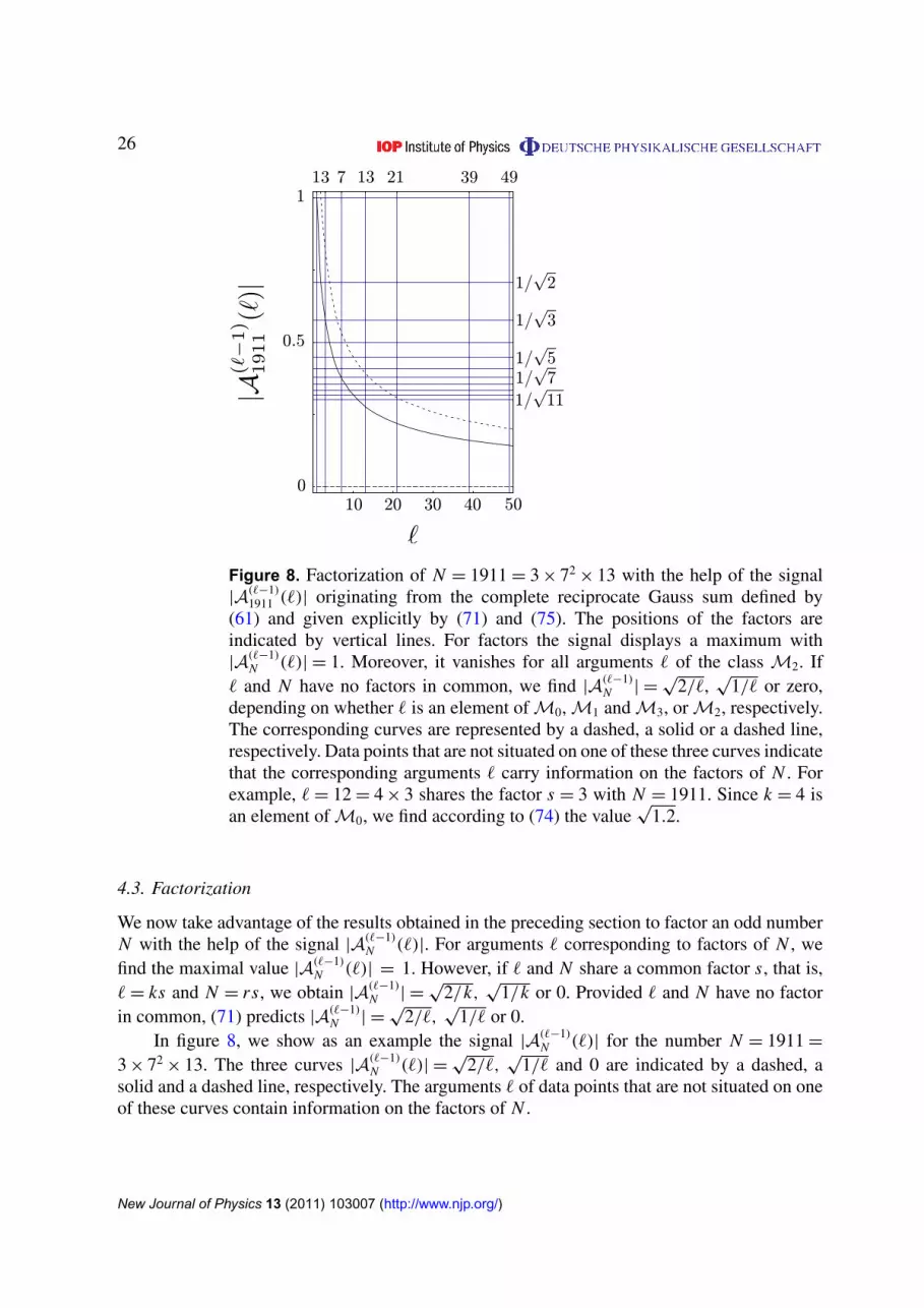
|A(`−1)1911 (`)| originating from the complete reciprocate Gauss sum defined by

(61) and given explicitly by (71) and (75). The positions of the factors areindicated by vertical lines. For factors the signal displays a maximum with|A(`−1)

N (`)| = 1. Moreover, it vanishes for all arguments ` of the class M2. If` and N have no factors in common, we find |A(`−1)

N | =√

2/`,√

1/` or zero,depending on whether ` is an element ofM0,M1 andM3, orM2, respectively.The corresponding curves are represented by a dashed, a solid or a dashed line,respectively. Data points that are not situated on one of these three curves indicatethat the corresponding arguments ` carry information on the factors of N . Forexample, `= 12 = 4 × 3 shares the factor s = 3 with N = 1911. Since k = 4 isan element ofM0, we find according to (74) the value

√1.2.

4.3. Factorization

We now take advantage of the results obtained in the preceding section to factor an odd numberN with the help of the signal |A(`−1)

N (`)|. For arguments ` corresponding to factors of N , wefind the maximal value |A(`−1)

N (`)| = 1. However, if ` and N share a common factor s, that is,`= ks and N = rs, we obtain |A(`−1)

N | =√

2/k,√

1/k or 0. Provided ` and N have no factorin common, (71) predicts |A(`−1)

N | =√

2/`,√

1/` or 0.In figure 8, we show as an example the signal |A(`−1)

N (`)| for the number N = 1911 =

3 × 72× 13. The three curves |A(`−1)

N (`)| =√

2/`,√

1/` and 0 are indicated by a dashed, asolid and a dashed line, respectively. The arguments ` of data points that are not situated on oneof these curves contain information on the factors of N .

New Journal of Physics 13 (2011) 103007 (http://www.njp.org/)

27

5. Conclusions and discussion

In the present article, we have analyzed different schemes to factor numbers based on threeclasses of Gauss sums. We have developed analytical criteria for deducing the factors of anumber N from a physical signal given by a Gauss sum, and have demonstrated the suggestedschemes by numerical examples. The continuous version of Gauss sum factorization has aremarkable scaling property. As a result, a single realization of the Gauss sum for the numberN yields information on the factors of another number N ′. The discrete version of this schemerests solely on the analysis of Gauss sums at integer arguments. The Gauss reciprocity relationallowed us to establish a link with yet another type of Gauss sum. Here, the roles of the argumentand the number to be factored are interchanged.

Unlike Shor’s algorithm, the factorization schemes discussed in this paper do not featurea reduction of the computational resources. Nevertheless, we are convinced that this approachwill open new perspectives on the connection between physics and number theory [20, 53]. Inparticular, our work is motivated by the search for physical systems that reproduce Gauss sums.In this spirit, the results of this paper provide the mathematical background for part II, wherewe address physical realizations of Gauss sums.

Acknowledgments

We have profited from numerous fruitful discussions with M Arndt, W B Case, B Chatel,C Feiler, M Gilowski, D Haase, M Yu Ivanov, E Lutz, H Maier, M Mehring, A A Rangelov,E M Rasel, M Sadgrove, Y Shih, M Stefanak, D Suter, V Tamma, S Weber and M S Zubairy.We thank D Suter for making his article [5] available to us before publication. WM and WPSacknowledge financial support from the Baden-Württemberg Stiftung. WPS also thanks theAlexander von Humboldt Stiftung and Max-Planck-Gesellschaft for support through the Max-Planck-Forschungspreis. IShA thanks the Israel Science Foundation for supporting this work.This work has also profited immensely from the stimulating atmosphere of the Ulm GraduateSchool Mathematical Analysis of Evolution, Information and Complexity under the leadershipof W Arendt.

Appendix A. Quantum algorithm for the phase of a Gauss sum

In this appendix, we briefly summarize a quantum algorithm [39, 40] proposed by W van Damand G Seroussi, which evaluates the phase of a certain class of Gauss sums. We compare andcontrast these Gauss sums with the ones central to our paper. Since the algorithm relies heavilyon the properties of multiplicative characters, we also briefly recall identities.

A.1. Gauss sums over rings

Gauss sums over a finite ring consisting of integers modulo n denoted by Z/nZ read

G(Z/nZ, χ, β)≡

n−1∑x=0

χ(x) exp

[2π i

βx

n

], (A.1)

where χ = χ(x) is a multiplicative character.

New Journal of Physics 13 (2011) 103007 (http://www.njp.org/)

28

The absolute value of G is given by

|G(Z/nZ, χ, β)| =√

n (A.2)

provided that n is prime. All other cases of n can be reduced to that one.In the present case study, the quadratic Gauss sum

G(a, b, c)≡

b−1∑m=0

exp[2π i

(m

c

b+ m2 a

b

)](A.3)

plays a central role. However, only for c = 0, gcd(a, b)=1 and b squarefree, which means thatb 6= n × q2, can we cast it into the form

G(a, b, 0)=

∑kεZ/bZ

(k

b

)exp

[2π i

ka

b

](A.4)

of a Gauss sum over a finite ring, where(

kb

)denotes the Legendre symbol. Hence, only in this

case can we perform the algorithm proposed in [39, 40].Furthermore, we note that for the quadratic Gauss sum G(a, b, 0), it is very easy to estimate

the phase γ , in contrast to the absolute value, which depends on the greatest common divisor ofa and c. In section 3, we use this attribute of quadratic Gauss sums to factor numbers.

A.2. Outline of the algorithm

In order to bring out most clearly the main principles of this phase-determining algorithm[39, 40], we choose the example of a finite ring Z/nZ over a prime n. If n is not prime, wehave to first find the factors of n and then execute the algorithm for each factor of n. With thehelp of the phases corresponding to each factor, it is possible [39, 40] to estimate the phase ofthe Gauss sum.

Moreover, in the next section we establish the relation

G(Z/nZ, χ, β)= χ−1(β)G(Z/nZ, χ, 1), (A.5)

which shows that it suffices to find the phase of G(Z/nZ, χ, 1) rather than G(Z/nZ, χ, β).With the help of Shor’s discrete log algorithm [61], the phase γ1 of χ−1(β) can be calculated inan efficient way. Hence, we are left with the task of finding the phase γ2 of G(Z/nZ, χ, 1).

The algorithm proceeds in four steps: first, we prepare the superposition state

|ψ〉 ≡1

√2(|�〉 + |χ〉) (A.6)

consisting of the state

|χ〉 ≡1

√n − 1

n−1∑x=0

χ(x)|x〉, (A.7)

and the ‘stale’ component |�〉. We emphasize that |χ〉 is a superposition of only n − 1orthonormalized states |x〉 since χ(0)= 0 as shown in the next section.

In the next step, we perform a quantum Fourier transformation (QFT)

UQFT|x〉 ≡1

√n

n−1∑y=0

exp[2π i

xy

n

]|y〉 (A.8)

New Journal of Physics 13 (2011) 103007 (http://www.njp.org/)

29

of |χ〉, which leads us to

UQFT|χ〉 =1

√n(n − 1)

n−1∑y=0

n−1∑x=0

χ(x) exp[2π i

xy

n

]|y〉. (A.9)

With the help of the definition of G, (A.1), we arrive at

UQFT|χ〉 =1

√n(n − 1)

n−1∑y=0

G(Z/nZ, χ, y)|y〉, (A.10)

which reduces with the identity (A.5) to

UQFT|χ〉 =G(Z/nZ, χ, 1)

√n(n − 1)

n−1∑y=0

χ−1(y)|y〉. (A.11)

In the third step, we produce the phase shift

Up|y〉 ≡ χ2(y)|y〉 (A.12)

on the basis states |y〉, which yields

Up UQFT |χ〉 =G(Z/nZ, χ, 1)

√n

|χ〉. (A.13)

Here, we have used again the definition of G, (A.1).The ‘stale’ component |�〉 is invariant under UQFT and Up. As a result the transformed

superposition state |ψ〉 = Up UQFT|ψ〉 reads

|ψ〉 =1

√2

(|�〉 +

G(Z/nZ, χ, 1)√

n|χ〉

), (A.14)

which due to expression (A.2) for the absolute value of G takes the form

|ψ〉 =1

√2(|�〉 + eiγ2|χ〉), (A.15)

where γ2 denotes the phase of G.In the fourth and final step, we implement, with the help of the initial superposition state

|ψ〉 (A.6) and the transformed state |ψ〉 (A.15), an algorithm for determining the phase γ2.In [39, 40], it is shown that this algorithm consisting of state preparation, QFT, creation of

phase shift and phase estimation can be performed in polylogarithmic time.

A.3. Properties of multiplicative characters

In this section we verify the identity

G(Z/nZ, χ, β)= χ−1(β)G(Z/nZ, χ, 1), (A.16)

which is crucial to the algorithm discussed in the preceding section. For this purpose we firstderive some properties of multiplicative characters and then use them to establish (A.16).

We start with the identity

χ(xy)= χ(x)χ(y) (A.17)

New Journal of Physics 13 (2011) 103007 (http://www.njp.org/)

30

of the multiplicative character χ , which for y ≡ 1 yields

χ(x · 1)= χ(x)= χ(x)χ(1), (A.18)

that is,

χ(1)= 1. (A.19)

Likewise, we find from (A.17) for y ≡ 0 the relation

χ(x · 0)= χ(0)= χ(x)χ(0), (A.20)

which is only true for arbitrary x provided

χ(0)= 0. (A.21)

Next, we substitute y ≡ x−1 into (A.17) and arrive at

χ(1)= χ

(x

1

x

)= χ(x)χ(x−1), (A.22)

which with the help of (A.19) reduces to

χ(x−1)= χ−1(x). (A.23)

As a consequence, we obtain the relation

χ(xβ−1

)= χ (x) χ

(β−1

)= χ(x)χ(β)−1. (A.24)

We are now in position to verify the identity (A.16). For this purpose, we introduce thesummation index y ≡ βx in the Gauss sum, (A.1), which reads

G(Z/nZ, χ, β)=

n−1∑y=0

χ(yβ−1) exp[2π i

y

n

]. (A.25)

Here, we emphasize that the summation has not changed due to the modular structure of thedomain of arguments x of the Gauss sum.

With the help of (A.24) and the definition (A.1) of G, we immediately arrive at (A.16).

Appendix B. Factorization with an N-slit interferometer

In this appendix, we summarize the essential ingredients of the pioneering proposal [49] by J FClauser and J P Dowling to factor odd numbers using a Young N -slit interferometer. For a moreelementary argument, see the appendix of [62].

We operate the interferometer with matter waves whose propagation is governed by theSchrödinger equation rather than light waves, whose evolution is described by the Maxwellequations. Needless to say, in the paraxial limit both wave equations agree.

We first derive an expression for the wave function on a screen located at a distance z froman N-slit grating with the period d . Screen and grating are parallel to each other. We then castthe Green’s function into a form that allows us to derive a criterion for the factorization of anodd integer N . Here, we use a property of Gauss sums derived in appendix C.

New Journal of Physics 13 (2011) 103007 (http://www.njp.org/)

31

B.1. Wave function on the screen

For the propagation of the initial wave function

ψ0(x)≡ ψ(x, 0)≡

N−1∑n=0

φ(x − nd) (B.1)

representing an array of N identical wave functions φ = φ(x) separated by d, we start from theHuygens integral [22]

ψ(x, t)=N (t)∫

∞

−∞

dy eiα(t)(x−y)2ψ0(y) (B.2)

for matter waves. Here we have introduced the abbreviation

α(t)≡M

2ht(B.3)

together with

N (t)≡

√α(t)

iπ(B.4)

and M denotes the mass of the particle.We substitute the initial wave function, (B.1), into the Huygens integral, (B.2), and

introduce the new integration variable ζ ≡ y/d − n, which yields

ψ(x, t)=

∫∞

−∞

dζ G( x

d− ζ, t

)φ(dζ ), (B.5)

where

G(ξ, t)≡ d N (t)N−1∑n=0

eiα(t)d2(ξ−n)2 (B.6)

is the Green’s function of the N -slit problem with the dimensionless position variable ξ .When we can treat the motion along the z-axis classically, the time t translates into the

longitudinal position z via the identity

t =z

vz, (B.7)

where vz is the velocity along the z-axis.With the help of the de Broglie relation Mvz = h2π/λ containing the wavelength λ of the

matter wave together with the definition of α, (B.3), we establish the identity

α(t)= α

(z

vz

)=

Mvz

2hz=π

λz(B.8)

and Green’s function, (B.6), takes the form

G

(ξ,

z

vz

)=

√d2

iλz

N−1∑n=0

exp

[iπ

d2

zλ(ξ − n)2

]. (B.9)

New Journal of Physics 13 (2011) 103007 (http://www.njp.org/)

32

We conclude by evaluating the Huygens integral, (B.5), in an approximate way. Wheneverφ = φ(x) is mainly concentrated around y = 0 and narrow compared to the smallest length scaleof G, we can evaluate G at ξ = 0 and factor it out of the integral, which leads us to

ψ

(x,

z

vz

)≈ φ G

(x

d,

z

vz

), (B.10)

where

φ ≡1

d

∫∞

−∞

dx φ(x). (B.11)

Hence, the intensity pattern |ψ(x, z/vz)|2 on the screen is mainly determined by the Green’s

function.

B.2. Different representations of the Green’s function

The factorization property [49] of the N -slit interferometer results from the periodicityproperties of the Green’s functionG, (B.9). To verify this claim, we now analyze the dependenceof G on λ.

Of particular importance is the situation when λ= ld2/z, where l is an integer. In this case,G given by (B.9) reduces to

G=

√1

il

N−1∑n=0

exp

[iπ

1

l(ξ − n)2

]. (B.12)

It is instructive to decompose the complete square in the phase into the individualcontributions and cast the sum in the form

G= ei8G, (B.13)

where

8≡π

lξ 2

−π

4, (B.14)

G ≡

√1

l

N−1∑n=0

exp(−2π i

n

lξ)γn (B.15)

with

γn ≡ exp

(iπ

n2

l

). (B.16)

Since the phase factor γn satisfies the periodicity property

γn+l = exp (iπl) γn, (B.17)

it is useful to represent the number N to be factored as a multiple k of l plus a remainder r , thatis, N = kl + r .

Similarly, the summation index n can be decomposed as n = jl + p. This property suggeststo express the sum over n into a double sum where the sum over j covers the k periods of lengthl and the one over p contains the elements of a single period. In the case l is not a factor of

New Journal of Physics 13 (2011) 103007 (http://www.njp.org/)

33

N , that is, when r is non-vanishing, there will be a remainder R due to the summation over anincomplete unit cell. Indeed, we arrive at

G =

√1

l

k−1∑j=0

l−1∑p=0

exp

[−2π i

jl + p

lξ

]γ jl+p +R(ξ) (B.18)

with

R(ξ)≡

√1

l

r−1∑p=0

exp

[−2π i

kl + p

lξ

]γkl+p. (B.19)

Due to the periodicity property (B.17), we find γ jl+p = exp[iπ jl] γp and the two sums in Gover j and p decouple. As a result G takes the form

G(ξ)=W (l)(ξ)1k(ξ − l/2)+R(ξ), (B.20)

where we have introduced the abbreviations

W (l)(ξ)≡

√1

l

l−1∑p=0

exp

[2π i

(p2 1

2l− p

ξ

l

)](B.21)

and

1k(ζ )≡

k−1∑j=0

exp[−2π i jζ ]. (B.22)

Moreover, the remainder R reduces to

R= exp [−2π ik(ξ − l/2)]

√1

l

r−1∑p=0

exp

[2π i

(p2

2l− p

ξ

l

)]. (B.23)

When we compare the sums in W (l) and the remainder R given by (B.21) and (B.23) wefind that they only differ in their upper limits. Indeed, the summation in W (l) extends over theperiod l, whereas the one in R only contains r terms.

B.3. Criterion for factorization

Since the function1k =1k(ζ ) is sharply peaked when ζ is an integer s, the Green’s function Ghas maxima at positions ξ = l/2 + s. Because N is odd, l must be also odd in order to be a factorof N . Hence, the phases interfere constructively at half-integers, that is, at ξ = q + 1/2 where qis an integer.

The weight of the peaks is given by |W (l)(ξ = q + 1/2)|2. As shown in appendix C it isequal to unity independent of q.

We therefore arrive at the following criterion [49] for finding factors of an odd number N :if l is a factor of N , the remainderR vanishes and the diffraction pattern consists of spikes at thepositions x = (q + 1/2)d of identical height. If l is not a factor of N the remainder R leads todiffraction patterns, which interfere with these spikes. As a result, their heights are not identicalanymore.

New Journal of Physics 13 (2011) 103007 (http://www.njp.org/)

34

Appendix C. Absolute value of a finite Gauss sum

In the factorization schemes based on the continuous Gauss sum SN (ξ) and the N -slitinterferometer discussed in section 2 and appendix B, respectively, the relation

|W (r)(a, b, c)|2 =1

r(C.1)

for the sum

W (r)(a, b, c)≡1

r

r−1∑p=0

exp

[iπ

r

(p2a + 2bp + pc

)](C.2)

plays a central role. It is noteworthy that (C.1) holds true for any integers a, b and c provided aand r are coprime and ar − c even. In the present appendix, we verify (C.1).

For this purpose, we first note that W (r) is periodic in b with period r . As a result we canexpand |W (r)

|2 into a Fourier series

|W (r)(a, b, c)|2 =1

r

r−1∑n=0

A(r)(n) exp

[−2π i

b

rn

](C.3)

with the expansion coefficients

A(r)(n)≡

r−1∑b=0

|W (r)(a, b, c)|2exp[2π i

n

rb]. (C.4)

In the second step, we substitute the definition (C.2) of W (r) into this expression for A(r)(n) andfind that

A(r)(n)=1

r 2

r−1∑p,p′=0

exp

[iπ

r

(p2a − p′2a + pc − p′c

)]1(p − p′ + n). (C.5)

Here, all terms containing the variable b are combined in

1(s)≡

r−1∑b=0

exp[2π i

s

rb]

=

{r, for s = k · r,0, else.

(C.6)

Because 06 p, p′, n < r , there are only two possibilities for which 1(p − p′ + n) is non-vanishing: p − p′ + n = 0 or p − p′ + n = r . In the first case, p must be smaller than r − nbecause p′ < r . In the second case p must be larger than or equal to r − n because 06 p′.Therefore, the Fourier coefficients given by (C.5) reduce to

A(r)(n)=1

r

r−n−1∑p=0

exp[−iπ

r

(2pna + an2 + nc

)]

+1

r

r−1∑p=r−n

exp[−iπ

r

(2pna + an2 + nc

)]e−π i(ar−c). (C.7)

If ar − c is an even number, we can combine these two sums into one sum

A(r)(n)=1

r

r−1∑p=0

exp[−2π i

na

rp]

exp

[−

iπ

r(an2 + nc)

], (C.8)

New Journal of Physics 13 (2011) 103007 (http://www.njp.org/)

35

which yields

A(r)(n)=

{1, for n = 0,0, else.

(C.9)

In the last step, we have used the fact that a and r are coprime.When we now substitute (C.9) into the Fourier representation (C.3), we immediately arrive

at (C.1).We conclude by analyzing the finite Gauss sum

W (r)m ≡

1

r

r−1∑p=0

exp[2π i

(p2 q

r+ p

m

r

)], (C.10)

which is a special case of W (r). Indeed, a comparison of (C.2) and (C.10) allows us toidentify the parameters a = 2q, b = m and c = 0. However, the discussion is now slightly morecomplicated. If r is odd it cannot share a divisor with a = 2q and we can apply (C.1). In thiscase, only the Fourier term with n = 0 is non-vanishing. On the other hand, if r is even, it shareswith a = 2q the factor 2, and also the term

A(r)(n = r/2)=1

r

r−1∑p=0

exp[−2π iqp − iπ

qr

2

]= exp

[−iπ

qr

2

](C.11)

is non-vanishing. With the help of (C.3), we find that

|W (r)(2q,m, 0)|2 =1

r

(1 + exp

[−iπ

(qr

2+ m

)])(C.12)

can be either zero if qr/2 + m is odd, or 2/r if it is even.

References

[1] Merkel W, Wölk S, Schleich W P, Averbukh I Sh, Girard B and Paulus G G 2011 Factorization of numberswith Gauss sums: II. Suggestions for implementation with chirped laser pulses New J. Phys. 13 103008

[2] Lang S 1970 Algebraic Number Theory (New York: Addison-Wesley)[3] Shor P 1994 Proc. 35th Annu. Symp. on Foundations of Computer Science (Santa Fe, NM) ed S Goldwasser

(New York: IEEE Computer Society Press) pp 124–34[4] Wölk S 2011 Factorization with Gauss Sums (München: Dr Hut)[5] Li J, Peng X, Du J and Suter D 2011 An efficient deterministic quantum algorithm for the integer square-free

decomposition problem arXiv:1108.5848v1[6] Mehring M, Müller K, Averbukh I Sh, Merkel W and Schleich W P 2007 Phys. Rev. Lett. 98 120502[7] Mahesh T, Rajendran N, Peng X and Suter D 2007 Phys. Rev. A 75 062303[8] Peng X and Suter D 2008 Europhys. Lett. 84 40006[9] Gilowski M, Wendrich T, Müller T, Jentsch C, Ertmer W, Rasel E M and Schleich W P 2008 Phys. Rev. Lett.

100 030201[10] Sadgrove M, Kumar S and Nakagawa K 2008 Phys. Rev. Lett. 101 180502[11] Sadgrove M, Kumar S and Nakagawa K 2009 Phys. Rev. A 79 053618[12] Bigourd D, Chatel B, Schleich W P and Girard B 2008 Phys. Rev. Lett. 100 030202[13] Weber S, Chatel B and Girard B 2008 Europhys. Lett. 83 34008[14] Tamma V, Zhang H, He X, Garrucio A and Shih Y 2009 J. Mod. Opt. 56 2125

New Journal of Physics 13 (2011) 103007 (http://www.njp.org/)

36

[15] Tamma V, Zhang H, He X, Garrucio A, Schleich W P and Shih Y 2011 Phys. Rev. A 83 020304Tamma V, Alley C O, Schleich W P and Shih Y 2010 Found. Phys. doi:10.1007/s10701-010-9522-3

[16] Chatel B, Degert J, Stock S and Girard B 2003 Phys. Rev. A 68 041402[17] Chatel B, Degert J and Girard B 2004 Phys. Rev. A 70 053414[18] Iwaniec H and Kowalski E 2004 Analytic Number Theory (Providence, RI: American Mathematical Society)

Ireland K and Rosen M 1990 A Classical Introduction to Modern Number Theory (Heidelberg: Springer)[19] Davenport H 1980 Multiplicative Number Theory (New York: Springer)[20] See for example Maier H and Schleich W P 2012 Prime Numbers 101: A Primer on Number Theory

(New York: Wiley-VCH)[21] Born M and Wolf E 1997 Principles of Optics (Cambridge: Cambridge University Press)[22] Feynman R P and Hibbs A R 1965 Quantum Mechanics and Path Integrals (New York: McGraw-Hill)[23] Wheeler J A 1989 Phys. Today 42 24[24] Dowling J P, Schleich W P and Wheeler J A 1991 Ann. Phys., Lpz. 48 423[25] Merkel W, Mack H, Lutz E, Paulus G G, Girard B and Schleich W P 2007 Phys. Rev. A 76 023417[26] Zamith S, Degert J, Stock S, de Beauvoir B, Blanchet V, Bouchene M A and Girard B 2001 Phys. Rev. Lett.

87 033001Degert J, Wohlleben W, Chatel B, Motzkus M and Girard B 2002 Phys. Rev. Lett. 89 203003

[27] Leichtle C, Averbukh I Sh and Schleich W P 1996 Phys. Rev. A 54 5299Leichtle C, Averbukh I Sh and Schleich W P 1996 Phys. Rev. Lett. 77 3999

[28] Schleich W P 2001 Quantum Optics in Phase Space (Berlin: Wiley-VCH)[29] Berry M V and Goldberg J 1988 Nonlinearity 1 1[30] Berry M V 1988 Physica D 33 26[31] Case W B, Tomandl M, Deachapunya S and Arndt M 2009 Opt. Express 17 20966[32] Berry M V, Marzoli I and Schleich W P 2001 Phys. World 14 39[33] Schleich W P and Barnett S M 1993 Quantum phase and phase dependent measurements Phys. Scr. T48[34] Sanders B C 1992 Phys. Rev. A 45 7746[35] Vandersypen L, Steffen M, Breytan G, Yannoni C, Sherwood M and Chuang I 2001 Nature 414 883[36] Lanyon B, Weinhold T, Langford N, Barbieri M, James D, Gilchrist A and White A 2007 Phys. Rev. Lett.

99 250505[37] Zubairy M S 2007 Science 316 554[38] Mermin N D 2007 Phys. Today 60 8

Mermin N D 2007 Phys. Today 60 10[39] van Dam W and Seroussi G arXiv:quant-ph/0207131[40] van Dam W and Seroussi G 2003 Quantum Algorithms for Estimating Gauss Sums and Calculating Discrete

Logarithms http://cs.ucsb.edu/vandam/gausssumdlog.pdf[41] Childs A M and van Dam W 2011 Rev. Mod. Phys. 82 1[42] Matsutani S and Onishi Y 2003 Found. Phys. Lett. 16 325[43] Stefanak M, Merkel W, Mehring M and Schleich W P 2008 Proc. Int. Symp. on Contemporary Physics

ed J Aslam and F H Riazuddin (Singapore: World Scientific) pp 87–94[44] Rangelov A A 2009 J. Phys. B: At. Mol. Opt. Phys. 42 021002[45] Jones J A 2008 Phys. Lett. A 372 5758[46] Wölk S, Feiler C and Schleich W P 2009 J. Mod. Opt. 56 2118[47] Stefanak M, Merkel W, Schleich W P, Haase D and Maier H 2007 New J. Phys. 9 370[48] Stefanak M, Haase D, Merkel W, Zubairy M S and Schleich W P 2008 J. Phys. A: Math. Theor. 41 304024[49] Clauser J F and Dowling J P 1996 Phys. Rev. A 53 4587[50] Summhammer J 1997 Phys. Rev. A 56 4324[51] Mack H, Bienert M, Haug F, Freyberger M and Schleich W P 2002 Phys. Status Solidi b 233 408[52] Mack H, Bienert M, Haug F, Straub F S, Freyberger M and Schleich W P 2002 Experimental Quantum

Computation and Information ed F De Martini and C Monroe (Amsterdam: IOS Press)[53] Merkel W et al 2006 Int. J. Mod. Phys. B 20 1893

New Journal of Physics 13 (2011) 103007 (http://www.njp.org/)

37

[54] Merkel W, Averbukh I Sh, Girard B, Paulus G G and Schleich W 2006 Fortschr. Phys. 54 369–84[55] Shapiro E A, Spanner M and Ivanov M Yu 2003 Phys. Rev. Lett. 91 237901[56] Spanner M, Shapiro E A and Ivanov M Yu 2004 Phys. Rev. Lett. 92 093001[57] Harter W G 2001 Phys. Rev. A 64 012312

Harter W G 2001 J. Mol. Spectrosc. 210 166[58] Ng H T and Nori F 2010 Phys. Rev. A 82 042317[59] Stenholm S 2007 private communication[60] Hannay J H and Berry M V 1980 Physica D 1 267[61] Shor P 1997 SIAM J. Comput. 26 1484[62] Mack R, Schleich W P, Haase D and Maier H 2009 Mathematical Analysis of Evolution, Information and

Complexity ed W Arendt and W P Schleich (Weinheim: Wiley-VCH) pp 395–431

New Journal of Physics 13 (2011) 103007 (http://www.njp.org/)