Embed Size (px)
Citation preview
Facu l t ad de C i enc i a s
Breath Figures Formation
José Manuel Guadarrama Cetina

S c h o o l o f S c i e n c e
Breath Figures Formation
Submitted by José Manuel Guadarrama Cetina in partial fulfillment of the require-ments for the Doctoral Degree of the University of Navarra
This dissertation has been written under my supervision in the Doctoral Program inComplex Systems, and I approve its submission to the Defense Committee.
Signed on January 22, 2013
Dr. Wenceslao González-Viñas

Declaración:Por la presente yo, D. José Manuel Guadarrama Cetina, declaro que esta tesis es frutode mi propio trabajo y que en mi conocimiento, no contiene ni material previamentepublicado o escrito por otra persona, ni material que sustancialmente haya formadoparte de los requerimientos para obtener cualquier otro título en cualquier centro deeducación superior, excepto en los lugares del texto en los que se ha hecho referenciaexplícita a la fuente de la información.
(I hereby declare that this submission is my own work and that, to the best of my knowl-edge and belief, it contains no material previously published or written by another per-son nor material which to a substantial extent has been accepted for the award of anyother degree of the university or other institute of higher learning, except where dueacknowledgment has been made in the text.)
De igual manera, autorizo al Departamento de Física y Matemática Aplicada de la Uni-versidad de Navarra, la distribución de esta tesis y, si procede, de la “fe de erratas” cor-respondiente por cualquier medio, sin perjuicio de los derechos de propiedad intelectualque me corresponden.
Signed on January 22, 2013
José Manuel Guadarrama Cetina
c José Manuel Guadarrama Cetina
Derechos de edición, divulgación y publicación:c Departamento de Física y Matemática Aplicada, Universidad de Navarra


A Dalia y Vladimir

Acknowledgements
Agradezco a mi esposa Dalia por haber aceptado este difıcil reto y por haberme apoyado y
acompanado todo este tiempo desde la distancia.
Agradezco a mi director de tesis Prof. Dr. Wenceslao Gonzalez-Vinas por confiar en mi
capacidad para la realizacion de la tesis, por sus finas atenciones durante estos casi cuatro anos
en Espana y su buen juicio en su direccion. A la Universidad de Navarra por recibirme y ofrecerme
un espacio para realizar mi proyecto de tesis doctoral. A la beca de Asociacion de Amigos por
todo el apoyo brindado durante este periodo de formacion tan importante. Al Profesor Dr. Javier
Burguete y a los profesores e investigadores del Departamento de Fısica y Matematica Aplicada.
En especial al Dr. Diego Maza de esta misma institucion por la ayuda prestada en la realizacion
de las fotografıas que aparecen en las Figuras 4.23 a 4.25. Al Gobierno espanol (FIS2008-01126,
FIS2011-24642) y al de Navarra por la financiacion parcial de los proyectos en los que esta inscrita
esta tesis.
My cordial thanks to Dr. Ramchandra Narhe for his huge collaboration and his advices on
this thesis work.
My cordial thanks to Prof. Dr. Daniel Beysens and Prof. Dr. Anne Mongruel for the
opportunity to work at the ESPCI-Paristech and all the rich discussion that have until now
maintained.
Agradezco al Profesor Gerardo Ruiz por el apoyo recibido durante las estancias realizadas en
el Taller de Fluidos de la Facultad de Ciencias de la UNAM, Mexico. Tambien agradezco a Sergio
Hernandez Zapata por su apoyo en el laboratorio.
Agradezco tambien a mis companeros doctorandos y colegas: Ana, Celia, Raheema, Neus,
Sara, Hugo, Ivan, Manuel, Miguel, Moorthi, por las largas horas de discusion companerismo.
Agradezco el enorme apoyo moral de mis padres y hermanas ya que sin ellos, no me hubiera
sido posible concretar este proyecto. En especial, quiero agradecer a mi hermana Lourdes y a su
esposo Mark Zalcik por su ayuda prestada durante la realizacion de esta tesis.
Agradezco a mi companero de piso Sachi por hacerme la vida facil en la ciudad de Pamplona.

Contents
Preface XI
1. Breath Figures 1
1.1. Introduction . . . . . . . . . . . . . . . . . . . . . . . . . . . . . . . . . . . . . . . . 1
1.2. Stages in the Dynamics of Breath Figures . . . . . . . . . . . . . . . . . . . . . . . 2
1.3. The Nucleation Stage . . . . . . . . . . . . . . . . . . . . . . . . . . . . . . . . . . 3
1.3.1. Homogeneous Nucleation . . . . . . . . . . . . . . . . . . . . . . . . . . . . 3
1.3.2. Heterogeneous Nucleation . . . . . . . . . . . . . . . . . . . . . . . . . . . . 5
1.4. The Intermediate Stage . . . . . . . . . . . . . . . . . . . . . . . . . . . . . . . . . 6
1.5. The Coalescence Stage . . . . . . . . . . . . . . . . . . . . . . . . . . . . . . . . . . 9
1.5.1. The Scaling Laws . . . . . . . . . . . . . . . . . . . . . . . . . . . . . . . . . 10
1.6. Another Model of BF Dynamics . . . . . . . . . . . . . . . . . . . . . . . . . . . . 11
2. Experimental Device and Tools for Image Analysis 13
2.1. Experimental Device . . . . . . . . . . . . . . . . . . . . . . . . . . . . . . . . . . . 13
2.1.1. Description of the Condensation Chamber . . . . . . . . . . . . . . . . . . . 13
2.2. Substrates, Substances, and Treatments . . . . . . . . . . . . . . . . . . . . . . . . 15
2.2.1. Physical Properties Values . . . . . . . . . . . . . . . . . . . . . . . . . . . . 17
2.3. Tools for Image Analysis . . . . . . . . . . . . . . . . . . . . . . . . . . . . . . . . . 18
2.3.1. Acquisition of Images . . . . . . . . . . . . . . . . . . . . . . . . . . . . . . 18
2.3.2. The Threshold Problem . . . . . . . . . . . . . . . . . . . . . . . . . . . . . 19
2.4. Errors . . . . . . . . . . . . . . . . . . . . . . . . . . . . . . . . . . . . . . . . . . . 21
2.4.1. The Error of Calculations with Matlab. . . . . . . . . . . . . . . . . . . . . 24
2.4.2. The Error of Calculations with ImageJ. . . . . . . . . . . . . . . . . . . . . 24
3. Breath Figures in Presence of a Humidity Sink 27
3.1. Introduction . . . . . . . . . . . . . . . . . . . . . . . . . . . . . . . . . . . . . . . . 28
3.2. Experimental Procedure . . . . . . . . . . . . . . . . . . . . . . . . . . . . . . . . . 29
3.2.1. Image Analysis . . . . . . . . . . . . . . . . . . . . . . . . . . . . . . . . . . 30
3.2.2. Integration Procedure for 〈r〉 . . . . . . . . . . . . . . . . . . . . . . . . . . 31
3.3. The Humidity Sink and the Depletion Zone . . . . . . . . . . . . . . . . . . . . . . 33
3.3.1. The Flux and the Depletion Zone . . . . . . . . . . . . . . . . . . . . . . . . 39
3.3.2. The Difference of Pressure around the Salty Drop . . . . . . . . . . . . . . 40
3.4. Drops Pattern Around the Humidity Sink . . . . . . . . . . . . . . . . . . . . . . . 43
ix
x CONTENTS
3.4.1. Mean Radius of the BF’s Droplets . . . . . . . . . . . . . . . . . . . . . . . 45
3.5. The Profile of the Pressure Gradient . . . . . . . . . . . . . . . . . . . . . . . . . . 47
3.6. Concluding Remarks . . . . . . . . . . . . . . . . . . . . . . . . . . . . . . . . . . . 50
4. Breath Figure under Solidification Temperature of Water 53
4.1. Introduction . . . . . . . . . . . . . . . . . . . . . . . . . . . . . . . . . . . . . . . . 54
4.2. Experimental Set Up and Procedures . . . . . . . . . . . . . . . . . . . . . . . . . . 55
4.3. Observations . . . . . . . . . . . . . . . . . . . . . . . . . . . . . . . . . . . . . . . 55
4.4. A Salty Drop under Solidification Temperature of Water:
Anisotropy on the Pressure Gradient. . . . . . . . . . . . . . . . . . . . . . . . . . 61
4.5. A Model of Ice Propagation . . . . . . . . . . . . . . . . . . . . . . . . . . . . . . . 65
4.5.1. Percolation . . . . . . . . . . . . . . . . . . . . . . . . . . . . . . . . . . . . 65
4.6. Summary and Concluding Remarks . . . . . . . . . . . . . . . . . . . . . . . . . . . 66
5. Two Immiscible Substances Condensing on a Cold Surface 79
5.1. Introduction . . . . . . . . . . . . . . . . . . . . . . . . . . . . . . . . . . . . . . . . 79
5.2. Experimental Procedure and General Observations . . . . . . . . . . . . . . . . . . 80
5.2.1. First Experiment: Single Vapor Condensation . . . . . . . . . . . . . . . . . 81
5.2.2. Second Experiment: Condensing one Vapor at once . . . . . . . . . . . . . 82
5.2.3. Third Experiment: Condensing Two Vapors Simultaneously . . . . . . . . . 83
5.3. Results . . . . . . . . . . . . . . . . . . . . . . . . . . . . . . . . . . . . . . . . . . . 83
5.4. Summary and Concluding Remarks . . . . . . . . . . . . . . . . . . . . . . . . . . . 102
Conclusions and Outlook 103
A. Appendix 1: Program Routines 105
A.1. Pre-analysis routines: Conversion PPM - JPEG . . . . . . . . . . . . . . . . . . . . 105
A.2. Salty-drop Analysis . . . . . . . . . . . . . . . . . . . . . . . . . . . . . . . . . . . . 108
B. Appendix 2: Characterization of the Condensation Chamber 119
B.1. Characterization . . . . . . . . . . . . . . . . . . . . . . . . . . . . . . . . . . . . . 119
C. Appendix 3: HVAC Diagram 123
Bibliography 125
Summary 129
Resumen 130
Preface
Objectives
The general objective of this work is to study the dynamics of water vapor condensation
over hydrophobic substrates in different conditions. Those conditions are: the presence of water
vapor sink, the lower temperature of solidification and a condensible but immiscible vapors. In
particular, the goal to start those studies was to build and provide an accurate image tool analysis
based in Matlab, Fortran and Octave routines. Concerning the water vapor condensation in
presence of a humidity sink, the goals were to describe the increment of water volume of the
humidity sink, the depletion zone formed around the sink [1]. Also the vapor pressure as a
function of water concentration on pattern outside of the depletion zone. We discovered a new
process of ice propagation [2] and the objective is to understand the phenomenon of propagation.
For the case of immiscible condensible vapors, the objective is to describe the dynamics of the
drop wise production and the aggregation of the two substances process into clusters [3].
The Breath Figures
Actually, my interest in Breath Figures arose when I received a positive answer from University
of Navarra to do my studies of PhD in complex systems. In addition, the idea of work with
thermodynamics calculations was enough to focus all my interest. The first time I have known
something of this phenomenon was after the shower, I stood in front the mirror to see the carpet
of the small droplets produced by the fog. I was trying to figure out how, when, where, and what
the difficulties could be on the study of such natural process. Of course, those thoughts were due
to the lack of experience. Three years after, my opinion at that respect have changed. When I
see a steamed mirror or a window, now I am trying to figure out what contact angle could it be.
This work is far from the assessments of thermodynamics, but it is fully formed of non linear
dynamics. Elsewhere in this work of thesis when I refer to Breath Figures (BF), I am referring
to water vapor condensing drop wise over a cold surface, and cold means the surface is kept at
lower temperature than the environment. I will remark the difference when I am talking about
other vapor substance different than water. Henceforth, Breath Figure will be (BF) and will
be exclusively for water vapor. The BF formation has three stages: 1) nucleation, 2) growth of
droplets only by condensation and no more nucleation appears, and 3) where coalescence events
rules the behavior of the dynamics and some time after, the growth, the renucleation of new
droplets which grow by condensation appear. Very good researches have done theory of high level
also, they have established the basis to describe a wide range of experimental observations. In
xi
xii Preface
addition, this work exhibits new design of configurations where is indispensable to apply many
resources of complex systems theory to explain the observations.
Context
The study of BF started in 1893 by the meteorologist J. Aitken [4, 5], and in 1911 by John
William Strutt (Lord Rayleigh) [6] ”After breathing on a window-pane we wrote our names on
the glass with the point of a finger. Now rater having waited until the moist deposit have
disappeared, and again breathing on the glass, the written characters became quite legible”.
Perhaps this was the first experiment related with hydrophobic surfaces and Breath Figure with
following conclusion ”This seems quite to agree with Lord Rayleigh’s explanation, grease on the
fingers causing the phenomenon.” At that time, to publish in Nature Journal appeared not
to be so complicated. However the really important issue to highlight is the fact that some
serious researches have begun to ask to themselves about what variables could be involved in this
phenomenon. Other interesting antecedent appeared in 1913 by John Aitken. He has explained
an experiment on surfaces carefully treated [7]. Nowadays, because huge efforts of many people,
some applications have been developed and technology of physical vapor deposition and also
technology of water vapor around its behavior.
Scope
The Breath Figure production is by itself an irreversible thermodynamic phenomenon out-
side of equilibrium. However, I am not handling my measurement and my analysis to give a
thermodynamic perspective. It is affordable of course but, to use the increment of the size of
the droplets, the variations of the temperature, as well, the boundaries conditions values of su-
persaturation pressure. With all these information we try to describe the growth and its time
evolution with meaning depth into the complexity of this phenomenon. The experiment features
can fit on chemistry, physical chemistry, engineering applications, physics theory, simulations, or
farthermost pure mathematics. The main feature of this work is the application of dynamics to
provide descriptions of liquid-solid interface interactions.
Some questions have arisen when the BF about the gradient vapor pressure distribution on
the vapor atmosphere close to the BF when interacts with a humidity sink. From the experi-
mental observations, we have carefully proceeded the image analysis in order to obtain geometric
measurements from the phenomenon. The values of partial pressures which are very difficult
to measure or detect, can be revealed by such analysis and throw diffusive equation. The low
dispersion on data let us to work with fittings and more imaginative and bold models. A new
configurations let us to observe and report a non discovered process on frost formation. The
properties of the evolution BF’s patterns under freezing water’s temperature at standard con-
ditions lead us to observe ice propagation as percolation process. This occurs when the three
water phases interact in small region. In other experiments (to following the logic stream) the
humidity sink is tested under frost phenomenon’s conditions to observe and afterward discover
the anisotropy of patterns can affect directly the salty drop’s growth.
It is a high priority to understand the mechanism of mixing two immiscible substances through
xiii
the population analysis of BF and condensation of other substance in the same cold surface from
image data. This phenomenology is very rich, because the population of droplets are sensitive
to heterogeneity or homogeneity on the spatial distributions. Actually, the coalescence’s theory
is very powerful and helpful to give ground to non classical growth’s laws and the complexity
behavior less studied on the specialized literature. Some theoretical already obtained results can
explain our own experimental observations. I am very confident on that theory with their scaling
laws and distributions functions help to understand the behavior and the tendencies. However
not all discoveries match with those results, and is where I am confident on my own observations
and measurements and, the wide possibilities to explain facts. With the philosophy ”the nature
has the last word overall cases”, I will to emphasize this study with only direct observations. I
will use the theory always to compare and to understand, and sometimes as a starting point of
analysis. Nevertheless, for some experiments, the results will not agree with theoreticians and
their calculations.
Outline
Concepts that belong to undergraduate level are left outside of this dissertation. There are
excellent bibliography almost anywhere. Instead, I pass directly to the substantial concepts. Each
chapter of this thesis work are thought in order to stand alone, and each one provides enough
information of the experiments, as well, as the theory used on the study.
In the introductory chapter 1, I display the content of general physics theory of Breath Figures
and I give a retrospective highlighted the results provided by the models and previous experiments.
In Chapter 2, I do the description of the experimental device used in this research. In the same
Chapter is signalized the troubleshooting on image analysis to extract a good (in statistical
way) amount of data. In Chapter 3, I give the physical description of experiment when a BF is
evolving in presence of a humidity sink. I use a simple model of flux to try to explain the depletion
zone around a salty drop. I report interesting results about the values of vapor partial pressure
obtained from direct measurements. In chapter 4, I report observations of a new discover process
on frost formation observed during a stage at the ESPCI-Paristech in Paris, France. When a BF
is produced over a surface at below temperature of solidification of water (−9 C). The water
droplets condensed are in a metastable phase of supercooled and by some perturbation a phase
transition occurs. The relevant observation is the percolation mechanism of ice propagation. As
well, evaporation of liquid droplets and vapor deposition are observed too. In Chapter 5, I report
experimental result when the vapor of two immiscible substances condense on the same repellent
surface. The measurements of the average radii and the coverage of the drops for each one evolve
with non classical growth laws. This situation is explained on the basis frame of scaling universal
relations.

xiv Preface
Chapter 1
Breath Figures
Figure 1.1: Breath Figures on my window in a cold morning.
1.1. Introduction
The phenomenon of Breath Figures (BF) is commonly found in nature and in our daily life.
It occurs when water vapor (WV) condenses as a dropwise process on a cold surface. When we
grab a bottle of some cold beverage out of the fridge in a hot day, we will immediately notice
that small droplets cover the surface of the glass. Another example is when we try to observe
ourselves in the mirror of the bathroom after taking a shower. The mirror will be covered with
”fog”. Physically, factors like the difference of the saturation pressures and the difference of
the temperatures between the water vapor and the glass can produce the transition onto liquid
phase. The next sections of this chapter are dedicated to explain the BF production. Theories,
simulations, and experiments have been done since the beginning of the 20th century. Nowadays,
solid-liquid interaction has been taking a rising interest in the discussion of this complex world
of BF’s patterns. The content written in this section is a compilation of those relevant studies.
In this chapter, the theory will provide the basis of understanding to obtain new results. Beyond
the theory described, other concepts will be cited and discussed later on.
1
2 Breath Figures
1.2. Stages in the Dynamics of Breath Figures
The properties of the surfaces play an important role in the formation of films and patterns.
Such properties are the surface dimension (can be modified) and the contact angle achieved at the
interface solid-liquid. The surface hydrophobicity (θc > 90) depends on the coatings, the micro
or nanometric etched patterns. The properties of wetting will also change if instead of a surface,
it is a porous medium, or a wire, like a spider web. As we will see, the phenomenon develops in
three general stages. There are exhaustive researches based on experiments and simulations since
1973 [8]. Those observations are affordable to develop in laboratory. I will not be the exception
here, all experiments reported in this work are related to the two stages of BF. I will give a
summary of what happens with those stages in a sequential order.
1. Nucleation stage There are two kind of nucleation processes: homogeneous and heteroge-
neous. The heterogeneous nucleation concept is fundamental to understand the formation
of dew. Now, it is considered the vapor at partial pressure Pss, which is larger than its
saturation pressure. It means that the vapor is in a metastable state and it will condense
into liquid phase, which is the state of minimum energy. The formation of liquid drops starts
by thermal fluctuations with the formation of thermodynamically stable small nuclei. The
small formed droplets are more stable than the water vapor and they do not evaporate. The
difference of temperatures between the supersaturated and the saturated vapor boosts the
system to pass an energy barrier and the water vapor condenses. The free energy ∆G for
spheric droplets can be written as [9]
∆G = −4
3πr3ρ
RT
µvlog
(
Ps
Pss
)
+ 4πr2γ (1.1)
where r, ρ, R, and T are the cluster radius, density, the gas constant and the temperature
define the change on volumetric energy required for the phase transition, µv, Ps, Pss and γ
are the molar mass, the partial pressures of saturation and supersaturation, and the surface
tension at the liquid vapor interface.
2. Growth stage. Here, all the nucleation sites have been occupied. The clusters formed
during the first stage, have formed drops. The new droplets will adsorb vapor on their
vicinity because of the difference of pressures with the atmosphere. The small droplets grow
without direct interaction (physical contact) among them and this is another characteristic
of the second stage of BF. The classical growth law1 for the average radius is [10],
〈r〉 ∼ t1/3 (1.2)
3. Coalescence stage. The third stage is governed by drop coalescence events. The main
characteristic is the self similar behavior. The drop’s s law of growth is proportional with t.
When droplets reach a certain size r, they start to interact with each others. They coalesce
and give away new droplets with new size [11],
r = (rD1 + rD2 )1/D (1.3)
1In Chapter 5 an experimental study of BF pattern with different growth law is included.
Section 1.3 3
where D is the drop dimension (usually three) and their mass center is the geometrical
mass center of two droplets. This is not totally true since it is possible to observe the
coalescence of more than two drops during the experiments. Even non spheric shape droplets
can be observed. In spite of this, the data analysis of many simulations and experimental
observations fit very well with this assumption. After the coalescence of two drops, there is
space released on the surface and a new BF could form among the bare spaces. The surface
occupation factor ǫ2 = (2〈r〉/〈a〉)2 behaves asymptotically towards a constant 0.55. That
means, that the distance distribution of droplets is (0.55〈a〉)1/2 = 2〈r〉 ≈ d
Another interesting proposal exists to describe the BF evolution such that, it is necessary to
include a fourth stage for long times [12]: after long times, many generations of droplets coexist
in this stage. The next section is a concise review of the nucleation process.
1.3. The Nucleation Stage
There are two types of nucleation2: the heterogeneous and the homogeneous nucleation. The
BF is an example of heterogeneous nucleation because the WV molecules nucleate on specific sites
on the substrate. The difference of pressures produces the impinging of the water molecules which
stick and aggregate on preferential sites. Concerning the homogeneous nucleation, the process is
totally different because there are not preferable sites to form the bulk.
1.3.1. Homogeneous Nucleation
Joseph Katz [13] has explained that homogeneous nucleation refers to the spontaneous creation
of a new phase3. The phase change may come from a parent metastable phase. Another interesting
example is the solidification of supercooled water. On this topic, A. Saito et al [14] and Tsutomu
Hozumi et al [15] have done research about this kind of nucleation. The solidification is also
observed in colloidal suspensions [16] and in the globular formation of proteins by hydrodynamic
mechanisms [17]. The homogeneous nucleation occurs within the supersaturated phase (gas, liquid
or solid) by the growth of embryos that have crossed a critical size. The size of those embryos can
achieve their super-critical size because of the impingement of monomers. A stationary condition
is assumed in order to explain that the reaction can occur at equilibrium concentration. In this
reaction the embryos and the monomers from the parent phase stay at the same temperature. In
classical theory of nucleation, the phenomenon can be interpreted with help of thermodynamics
and statistical physics.
∆G = ∆G(phase change) + ∆G(surface tension) (1.4)
If we consider the simplest case for vapor condensation, the partial pressure and the super-
saturation pressure provide boundary conditions for the nucleation process. The radii of clusters
and their surface energy can be determined by the free energy (Equation 1.1) which behaves as a
monotonically increasing function when (Ps/Pss) < 1.The vapor pressure under saturated condi-
tion is lower than the vapor pressure at supersaturated condition. If (Ps/Pss) > 1, condensation
2The analysis of nucleation process along the thesis work is not used because it is not in the goals and in the perspective
of this work. Withal, it is important to do a review to understand what the phenomenon of Breath Figures is.3This refers under the supersaturation condition.
4 Breath Figures
occurs. The initial increment of the cluster energy is due to the large value of the surface term.
When the clusters begin to increase this value becomes less important and the phase change is
imminent. The maximal free energy drives clusters to reach a critical radius r∗[18],
r∗ = [2σuv] /
[
ρRT ln
(
Pv
P∞
)]
, (1.5)
and this last (Equation 1.5) is known as Kelvin’s equation[16].
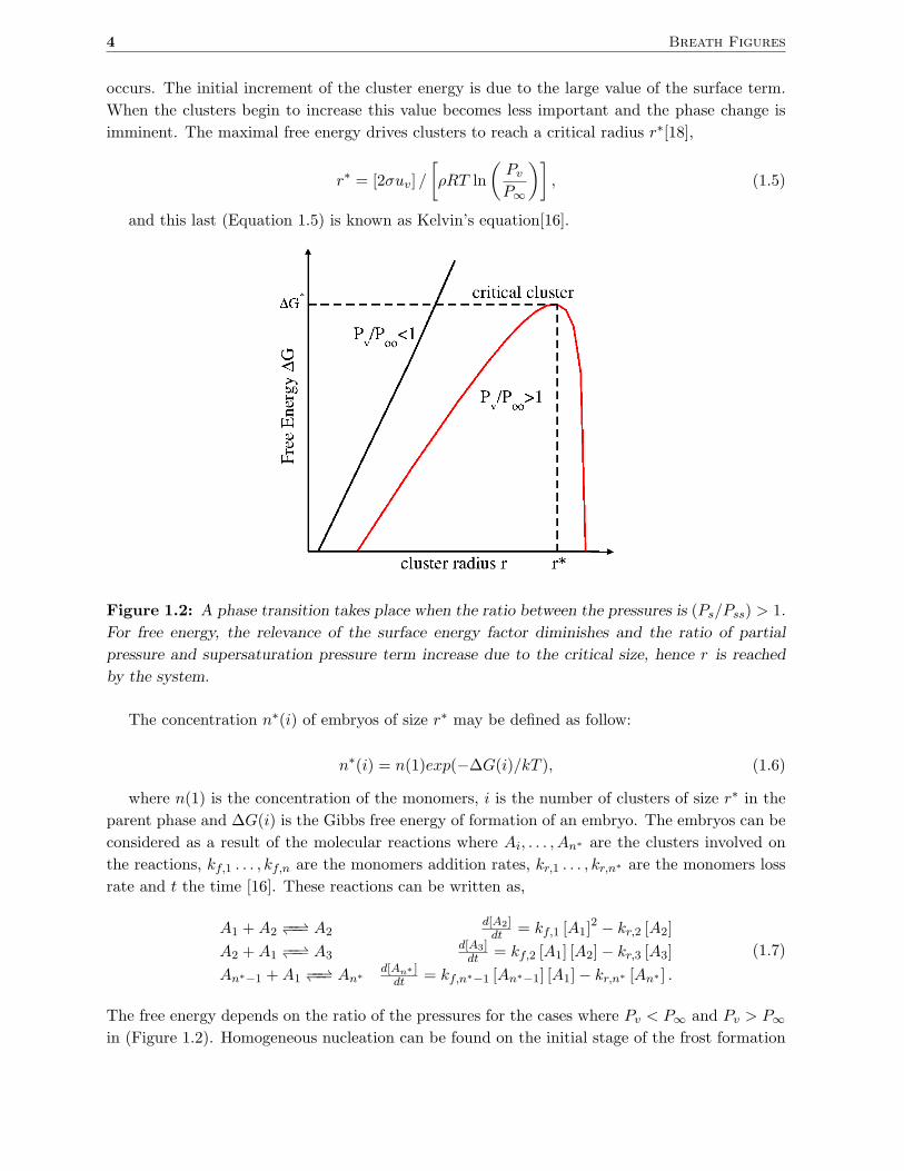
Figure 1.2: A phase transition takes place when the ratio between the pressures is (Ps/Pss) > 1.
For free energy, the relevance of the surface energy factor diminishes and the ratio of partial
pressure and supersaturation pressure term increase due to the critical size, hence r is reached
by the system.
The concentration n∗(i) of embryos of size r∗ may be defined as follow:
n∗(i) = n(1)exp(−∆G(i)/kT ), (1.6)
where n(1) is the concentration of the monomers, i is the number of clusters of size r∗ in the
parent phase and ∆G(i) is the Gibbs free energy of formation of an embryo. The embryos can be
considered as a result of the molecular reactions where Ai, . . . , An∗ are the clusters involved on
the reactions, kf,1 . . . , kf,n are the monomers addition rates, kr,1 . . . , kr,n∗ are the monomers loss
rate and t the time [16]. These reactions can be written as,
A1 +A2 −−−− A2d[A2]dt = kf,1 [A1]
2 − kr,2 [A2]
A2 +A1 −−−− A3d[A3]dt = kf,2 [A1] [A2]− kr,3 [A3]
An∗−1 +A1 −−−− An∗
d[An∗ ]dt = kf,n∗−1 [An∗−1] [A1]− kr,n∗ [An∗ ] .
(1.7)
The free energy depends on the ratio of the pressures for the cases where Pv < P∞ and Pv > P∞
in (Figure 1.2). Homogeneous nucleation can be found on the initial stage of the frost formation
Section 1.3 5
process (This can be linked to the topic of solidification of supercooled water in Chapter 4). In
meteorology, the clouds formation is a remarkable example of homogeneous nucleation because
all above conditions are present. In clouds, the phases of vapor, liquid and solid may coexist.
This means the cloud’s system presents activity when the liquid phase transforms into solid and
the vapor phase transforms into liquid. This process is called WBF since it was discovered by
Wegener, Bergeron, and Findeisen [19].
1.3.2. Heterogeneous Nucleation
Heterogeneous nucleation models require the establishment of embryos population at the equi-
librium of concentration of embryos and monomers in specific sites. The nucleation occurs on
liquids or solids that are in contact with surfaces or particles. The condensation and the diffusive
events are understood as the monomers’ aggregation to big molecules occupying a surface. Some
interesting observations of the heterogeneous nucleation stage have been performed through elec-
tron microscopy [20, 21]. In those references, the authors describe the nucleation by the Gibbs
energy as a function of the surface tension and geometric parameters (Equation 1.8 and Fig-
ure 1.3). The observations were done over superhydrophobic’s surface tension, low pressures
(∼100 Pa) and a temperature of -13 C.
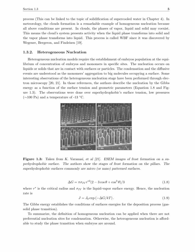
Figure 1.3: Taken from K. Varanasi, et al [21]. ESEM images of frost formation on a su-
perhydrophobic surface. The authors show the stages of frost formation on the pillars. The
superhydrophobic surfaces commonly are micro (or nano) patterned surfaces.
∆G = πσIV r∗2(2− 3 cos θ + cos3 θ)/3 (1.8)
where r∗ is the critical radius and σIV is the liquid-vapor surface energy. Hence, the nucleation
rate is
J = J0 exp (−∆G/kT ) . (1.9)
The Gibbs energy establishes the conditions of surfaces energies for the deposition process (gas-
solid phase transition).
To summarize, the definition of homogeneous nucleation can be applied when there are not
preferential nucleation sites for condensation. Otherwise, the heterogeneous nucleation is afford-
able to study the phase transition when embryos are around.
6 Breath Figures
Concerning the BF, the radius of a droplet rs in the nucleation stage is much smaller than its
distance neighbors rd. The new droplets collect vapor from the surroundings by surface diffusion.
This reduces the molecular concentration of the vapor. Thus, the droplets form an inhibition
region where no more nuclei of condensation can be found, so no new droplets appear there.
1.4. The Intermediate Stage
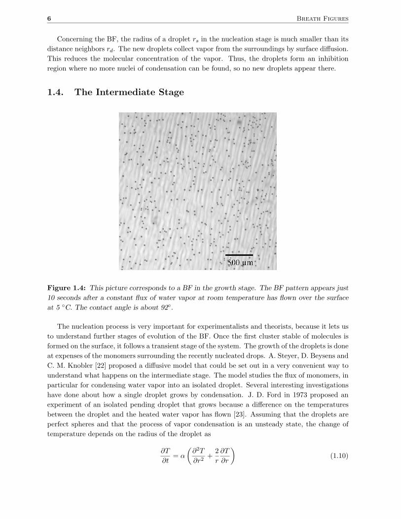
Figure 1.4: This picture corresponds to a BF in the growth stage. The BF pattern appears just
10 seconds after a constant flux of water vapor at room temperature has flown over the surface
at 5 C. The contact angle is about 92.
The nucleation process is very important for experimentalists and theorists, because it lets us
to understand further stages of evolution of the BF. Once the first cluster stable of molecules is
formed on the surface, it follows a transient stage of the system. The growth of the droplets is done
at expenses of the monomers surrounding the recently nucleated drops. A. Steyer, D. Beysens and
C. M. Knobler [22] proposed a diffusive model that could be set out in a very convenient way to
understand what happens on the intermediate stage. The model studies the flux of monomers, in
particular for condensing water vapor into an isolated droplet. Several interesting investigations
have done about how a single droplet grows by condensation. J. D. Ford in 1973 proposed an
experiment of an isolated pending droplet that grows because a difference on the temperatures
between the droplet and the heated water vapor has flown [23]. Assuming that the droplets are
perfect spheres and that the process of vapor condensation is an unsteady state, the change of
temperature depends on the radius of the droplet as
∂T
∂t= α
(
∂2T
∂r2+
2
r
∂T
∂r
)
(1.10)
Section 1.4 7
with the boundary conditions T (r, 0) = Tb for r << R (the initial radius r 6= 0) of the droplet.
T (R, t) = Ts t > 0, where Ts is the saturation temperature and ∂T∂r = 0 when r = 0 (for
symmetry). The authors have considered the heat flux at the condition r = R in order to solve
the Equation 1.10 by an approximation. The balance equation for heat at the interface liquid-
vapor is
k
(
∂T
∂r
)
r=R
= λρdR
dt. (1.11)
The Equation 1.11 is valid only at the singularity defined by the vapor-liquid interface. This
assumption is necessary to solve the problem of growth as a function of the temperature T . This
is very interesting because, there is no assumption of molecules concentration at any place. The
formal solution for T is
T = Ts + (Ts − Ti)2R
πr
∞∑
n=1
(−1)n
nsin
nπr
Rexp
−n2π2 αt
R2
. (1.12)
Solving the Equation 1.11, and applying Equation 1.12, at t = 0 and R = Ri it has been found
the ratio RRi
∼ 1+(1− exp f(t))1/2, where f(t) is the exponential function for n = 1. For t → ∞,
the ratio RRi
∼(
1 + CpTs−Ti
λ
)1/3describes the growth of an isolated drop pendant on air and
surrounded by vapor. This article [23] provides several experimental data of testing initial radii
and several differences of temperature. Another interesting investigation about the case when
an isolated drop settled on a surface and surrounded by vapor is given by Sokouler [24] the
condensation of a single drop can be treated as an inverted evaporation process. The growth law
for that drop should be V ∝ t3/2 without the effects of convection. In this case, the assumptions
require an environment of oversaturate constant vapor source, and volume relations require the
dependence on the spacing between the drops. When the reservoir of vapor is placed at a distance
similar to the mean drop separation d, in a steady state, the vapor flux through any area parallel
to the surface. The change of volume is,
dV
dt= J0Vmd2 (1.13)
where Vm is the molar flux, d2 is the mean square distance of the droplets. This agrees with D.
Beysens [25] who describes the growth of a drop’s carpet by surface diffusion. However, when
he considers an isolated drop, the Equation 1.14 describes the flux for certain radius outside the
drop.
2πd(r2Jr)
dr= 0 ⇒
dJrJr
= −2a
rdr. (1.14)
Here Jr is the total vapor flux, a is the radius of the droplet, and r is a radius whose starting
coordinate coincides with the center of the drop and its magnitude is comparable to d. The
essential idea is to set drop’s volume rate of change as a function of the vapor flux per unit of
area, but first, it is necessary to apply the relation of flux Jr on the Fick’s diffusion relation−→J = −D∇C to obtain
Jr = J0
( a
r2
)
∣
∣
∣
∣
b
a
= Da
r2(Ca − C∞) , (1.15)
8 Breath Figures
where J0 is the flux at the drop surface on a radial geometry a, C∞ and Ca < C∞ is the relation
of bulk concentration near and far from the drop. Again, the change of drop’s volume is analyzed
at the gas-liquid interface.dV
dt=
∫
JrdA, (1.16)
then,
V = η
[
4πDM
3ρRT(P∞ − Pa)
]3/2
t3/2, (1.17)
hence r ∼ t1/2. The experiments support this result. A. Steyer and D. Beysens [22] assume there
is a flux of monomers entering throw the contact line of an isolated droplet,
∂n
∂t= D
(
∂2n
∂r2+
1
r
∂n
∂r
)
. (1.18)
The droplet is a 3-dimension object and it is surrounded by monomers on a 2-dimension surface,
this assumption is also supported by T. M. Rogers, K. R. Elder and Rashmi C. Desai [26], where
the concentration gradient is depicted as,
V
(
2πRD∂n
∂r
)
= R2dR
dtwith:
n(r, t) = n0
R(t = 0) = 0
n(R, t) = 0
(1.19)
The Equation 1.18 is evaluated at the liquid-gas interface with the boundary conditions in Equa-
tion 1.19, where V contains information the contact angle and the volume of one monomer. Far
from the drop (at infinity), the flux of monomers φ is assumed constant. The spatial distribution
of monomers around the drop can be obtained from the steady solution of Equation 1.18,
n = A+B ln r, (1.20)
where A and B are constants. After applying the conditions (Equation 1.19), the explicit form
of monomers distribution becomes
n =φ
2πDln(r/R) (1.21)
and as a consequence of constant flux φ, the right side of the Equation 1.19, we have
R2R = φV, (1.22)
and right away the relation is obtained,
R ∼ t1/3. (1.23)
Similarly, other authors support the idea of the monomers that run in a 2-dimension surface like
P. L. Krapivsky [27]. This implies that the contact line plays the main role on the growth by
condensation. Based on a quasi static approximation, he predicts that the radius increases as
(t/ln(t))1/3. Some other aspects involved on heat and mass transfer can be reviewed on [28]. As I
mentioned above, something common during the early stages of condensation is that the droplets
are formed and grow very separated from each others Rd > Rs (Rs is the radius of a droplet
Section 1.5 9
and Rd the distance between neighbors). The droplets collect vapor by a diffusive process. This
reduces the concentration of the molecules of vapor adsorbed in those sites that have not been
occupied. Under this circumstances, the number of droplets is almost always constant.
dS
dt∼
1
N≃ const. (1.24)
where S is the average size of the droplet and N the number of droplets. In case of d =2 and
D =3, dRs/dt ∼ R−2 or Rs(t) ∼ t1/3.
1.5. The Coalescence Stage
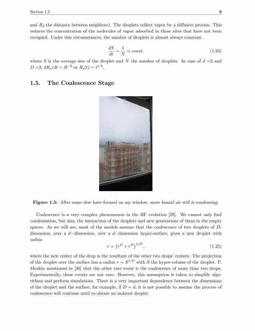
Figure 1.5: After some dew have formed on my window, more humid air still is condensing.
Coalescence is a very complex phenomenon in the BF evolution [29]. We cannot only find
condensation, but also, the interaction of the droplets and new generations of them in the empty
spaces. As we will see, most of the models assume that the coalescence of two droplets of D-
dimension, over a d−dimension, over a d−dimension hyper-surface, gives a new droplet with
radius
r =(
rD + rD)1/D
, (1.25)
where the new center of the drop is the resultant of the other two drops’ centers. The projection
of the droplet over the surface has a radius r ∼ S1/D with S the hyper-volume of the droplet. P.
Meakin mentioned in [30] that the other rare event is the coalescence of more than two drops.
Experimentally, these events are not rare. However, this assumption is taken to simplify algo-
rithms and perform simulations. There is a very important dependence between the dimensions
of the droplet and the surface, for example, if D = d, it is not possible to assume the process of
coalescence will continue until to obtain an isolated droplet.
10 Breath Figures
The coalescence events can be described in terms of the size s as following
ds
dt∼ s2/3, (1.26)
where s can be related with the drop’s radius as
dr
dt∼ const. (1.27)
1.5.1. The Scaling Laws
Fereydoone Family and Paul Meakin in [11] have established more general distribution func-
tions to describe the stage of coalescence. The authors remark the distinction between the ho-
mogeneous or heterogeneous nucleation on the analysis of the mean growth of the droplets. This
distinction is done because the referred work is based on simulation results. For those simulations,
the authors define an area substrate as Ld to condense vapors, to condense a defined number of
droplets in two configurations: in random and determined sites. Nevertheless, the following equa-
tions are valid for homogeneous nucleation and they are similar for a heterogeneous nucleation.
Here, the homogeneous term means the droplets are distributed on random sites and the term
heterogeneous is due to the selected sites for distribution of droplets. The difference between the
both points of view will be displayed below. Meanwhile, the mean size of droplets is
S(t) =
∑
s s2Ns(t)
∑
s sNs(t). (1.28)
The size relation with the average radius is R(t) ∼ S(t)1/D and this diverges as S(t) ∼ tz, and
R(t) ∼ tz/D (1.29)
where z depends on the droplet dimension D and the surface dimension d. The total number of
droplets N(t) decreases with the exponent z′
N(t) =∑
s
Ns(t) ∼ t−z (1.30)
It is possible to assume [31] that the number of droplets of size s at time t scales as
Ns(t) ∼ s−θf(s/S(t)), (1.31)
where f(x) is a bell-shaped function centered in x = 1 and with the form [30]
f(x) = x(θ−τ)g(x) + h(x). (1.32)
where g(x) decreases rapidly at any power of x as x → 0 and τ denotes the decay on smaller
droplets and θ is the scaling of the whole distribution and depends on d and D. The density
function proposed is
ρ =∑
s
sNs(t) ∼
∫
s1−θf(s/S(t)) ∼ S2−θ
∫
x1−θf(x) ∼ tz(2−θ), (1.33)
Section 1.6 11
Using the scaling form (Equation 1.31) in the definition of the density (Equation 1.33), we can
obtain directly that θ = 1 + d/D. The relation between θ and z is (θ + 1)/z = 2 for θ ≤2 with
z >0. As R is the only relevant parameter on the system, the exponent z is defined as
z =D
D − d. (1.34)
In case of heterogeneous nucleation, the equation which satisfying the defined initial sites are
pretty similardr
dt∝ rw (1.35)
and the growth of a single drop is r′ =(
rξ + δξ)1/ξ
with ξ = 1−w and r′ as the new value of the
radius, and w = 1 − D + d. The density function, now is re-written as ρ ∼ RD−d ∼ tz(D−d)/D.
An experimental discussion about this theory can be found in the R. D. Narhe and S. B. Ogale
[32]. This investigation shows some discrepancies on the analysis of the droplets size s and S(t)
obtained by two different mechanism of condensation.
1.6. Another Model of BF Dynamics
An analytic model for droplets growth consists in observing the diameter of droplets DA and
to consider three features of the self-similar regime.
For Briscoe and Galvin [33–35], the three stages of BF evolution are: the nucleation and
growth of the droplets just by condensation, and the coalescence with re-nucleation. The most
important aspect of this theory is the establishment of a differential equation to connect the
occupancy with the mean growth rate of the droplets. The drops diameter Di of intrinsic growth
can be generalized as
φIi =dDi
dt= kD−β
i (1.36)
with β as the intrinsic growth law exponent and k is assumed constant. Then, the fraction
occupation of the substrate in a certain area is
ǫ2 =
N∑
i=1
(π/4)D2i = N (π/4)D2
A, (1.37)
and taking into account Equation 1.36
NDAφIA = kN∑
i=1
D1−βi (1.38)
Hence, the intrinsic growth is obtained from dǫ2/dt (from Equation 1.38),
dǫ2
dt=
π
2(NDA)φNA + (π/4)D2
A
dN
dt. (1.39)
The following assumptions are necessary to establish the above differential equation:
a The geometry of the droplets is governed by the capillarity and the surface tension forces.
12 Breath Figures
b There is no hysteresis on the contact angle.
c The coalescence events are instantaneous.
d A coalescence event only involves two droplets.
e The initial size of the droplets is the same, their sites are random and there is not overlap of
droplets.
The Equation 1.39 and the relation π2 (NDA)φNA describe the increment of the occupation ǫ2
by the intrinsic growth, NφNA and DA are constants related to the growth of intrinsic droplets in
a respectively area. (π/4)D2A
dNdt denotes the growth due to the coalescence effect. The constant
(π/4)D2A is the expected change value on the area due to the coalescence events.
Chapter 2
Experimental Device and Tools for
Image Analysis
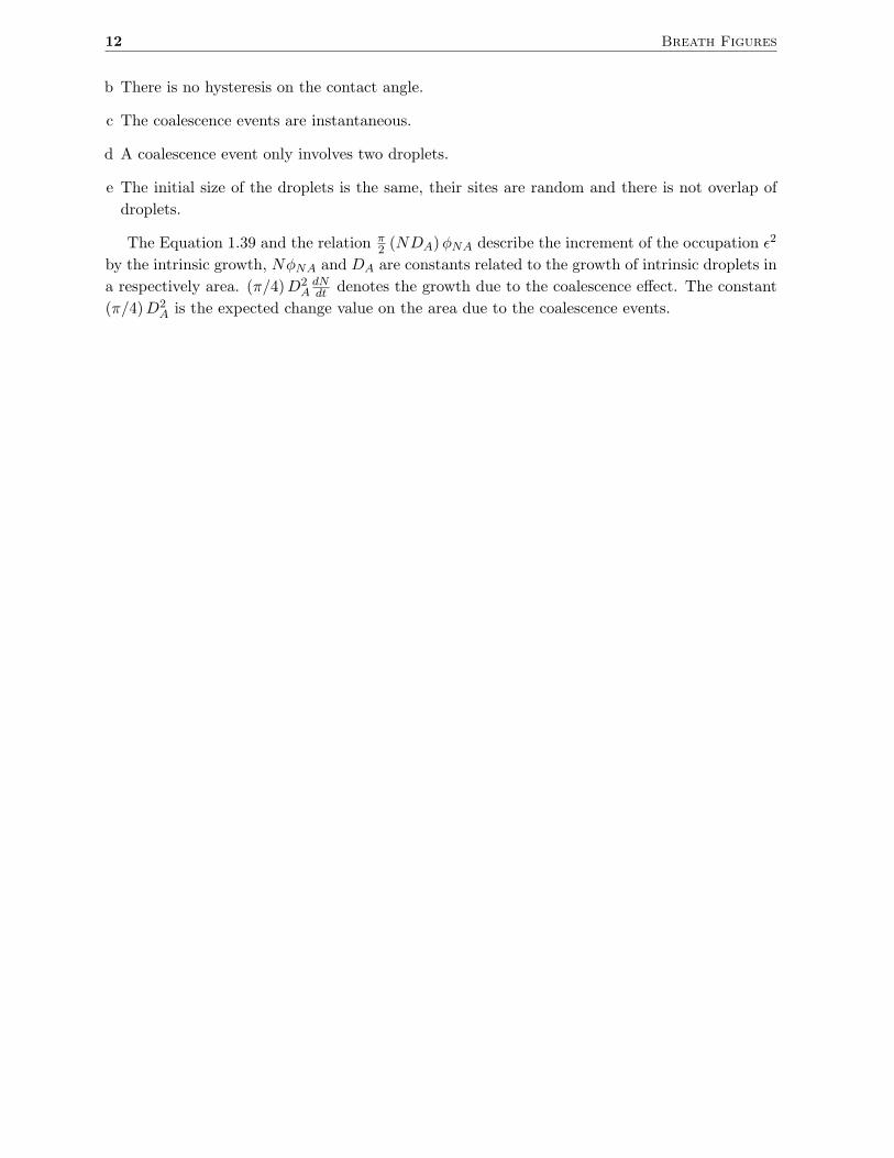
Figure 2.1: Experimental set-up
This chapter provides a description of the experimental device, and of, the physical properties
of the substances used to perform the experiments. The image analysis proceedings are described
too. We show on detail, the calculation of geometric properties and their uncertainties using
programs like ImageJ, Octave and Matlab.
2.1. Experimental Device
2.1.1. Description of the Condensation Chamber
The device can be described as a closed non hermetic chamber. It has three parts:
(1) In the top cavity, there is a cover with a non reflecting window. There are four inlets too (or
outlets, depending on the utilization). The inlets are placed every 90. The vapor flows in
a laminar flow regime at rates between 100 and 250 ml/min: the two faced inlets are used
to flow gases at the internal part of the chamber to have a stagnation point in the center.
At that place can be found established conditions and it is where the samples are set. The
13
14 Experimental Device and Tools for Image Analysis
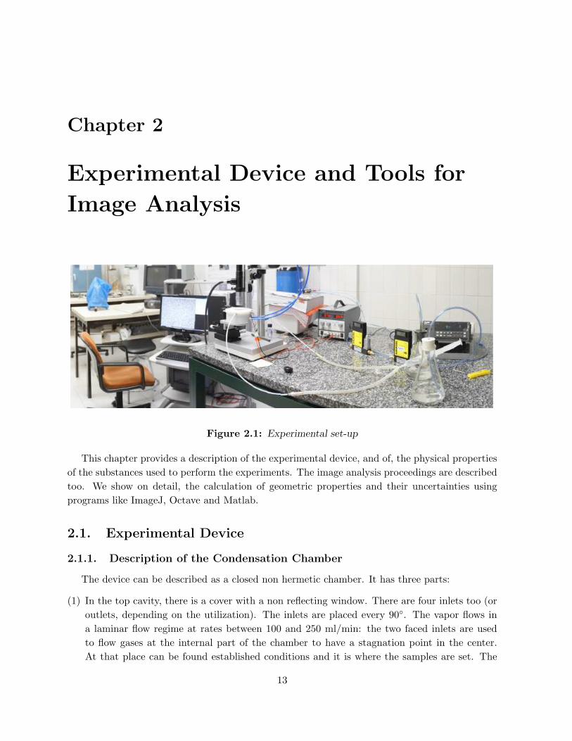
Figure 2.2: The Condensation Chamber. (A) Schematic view: (a) A post support of the
microscope. (b) The holders and supports of the in-line microscope and digital camera. (c)
The main tube to mount the microscope. (d) Translation stage X, Y , Z. (e) Weight to give
stability. (B) The schematic view of the condensation chamber: (1) Workplace to set samples
and to stream vapors. This places are divided by copper (good thermal conductor) plates. (2)
Room for a Peltier element. (3) A tank of recirculating water made of copper to dissipate the
heat extracted from the workplace. (C) The exterior of the chamber made of Delrin: (a) The
cover. (b) Window of anti-reflective glass. (c) There are two inlets and tubes to stream vapor
into the chamber, (d) And two inlets to do recirculation of cold water. (e) Thermocouples and
power source connections.
air flux is supplied by two AALBORG flux controllers which operate on the range of 0 to
500 ±0.2 ml/min. The inlets have an inner diameter of 2 mm and the associated Reynolds
number is ≈318. Moreover, in the Appendix 2 we show measurements of the velocity field
inside the chamber in order to characterize the hydrodynamical effects. Those measurements
were done by hot-wire velocimetry.
(2) There is a Peltier element inside of a small compartment that is beneath the workplace and a
copper tank. In the tank there is recirculating cold water (Figure 2.2B). With this device the
operation temperature can variate in a range -13 to 60 ±0.5 C. The operation temperature
depends on the polarity of the voltage operation. The Peltier element is a solid-state device
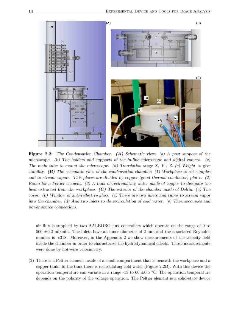
Section 2.2 15
that uses the Peltier’s effect to create a heat flux across the junction of two different types
of materials. This electronic component can be utilized as a heater or cooler. It transfers
heat from side to side against the temperature gradient when it is applied a electrical current.
The Peltier element on operation has an efficiency of an ideal refrigerator of 5 or 10 %. In
comparison with a reversible Carnot cycle it is very poor. Withal, its performance is enough
to keep constant on established operation temperatures. The size of this electronic component
are 3.4×3.4×0.4 cm3 and the input power to produce temperature difference of 65 C at 35
Watts (Figure 2.3).
(3) The chamber is mounted on a steel structure consisting of a post supporting an in-line micro-
scope with a support table base with possibility of micro metric stage X, Y , Z (Figure 2.2A).
Even though it is non a complex mechanism to operate, the system provides exceptional
stability condition to develop experiments of condensation of gases. The Delrin material and
the treated copper are resistant to the acid attacks and deformations (Figure 2.2C).
Figure 2.3: Peltier element extracts heat from a hot source to a sink by the action of electrical
current (left). An individual P −N solid-state array is shown (right).
2.2. Substrates, Substances, and Treatments
Many materials are hydrophobic like the polyurethane, and other plastics, silicon wafers, wax,
solid benzene, some carbon fibers, the zircon glass, the silane coated glass, etc. The chemical
etched metals or surfaces and the structured surfaces may increase the contact angle reducing
the contact area of liquid droplets. The glass has been coated with ITO (Indium Tin Oxide).
Also, it is a transparent conductive coating which can be used several times. Other substrates
used are glass cover slips coated with 3M EGC-1700 (or 3M). Due to its thinness, this substrate
is good to avoid thermal isolation effects. The 3M coated substrate and water develop a contact
angle of 92. The contact angle between the HMDSO C6H18OSi2 and 3M coating is 65. The
coating procedure is simple; just dipping the glass into the 3M and then wait for few minutes to
dry at room temperature. In some cases it is necessary to clean the substrates before using them.
In the specialized literature are many procedures and recipes for the substrate cleaning [36, 37].
Sometimes, those procedures are required to give an aggressive chemical thermal bath in order
to reorganize or alter the chemical bounds. For example when an ITO sample is cleaned with a
16 Experimental Device and Tools for Image Analysis
basic piranha bath, the hydrophobic property disappears awhile because the surface loses atoms
of oxygen therefore the contact angle is reduced. Other methods of cleaning substrates consist
only in washing the substrates with acetone, ultra-pure water or just ethanol in an ultrasonic
bath, then rinsing with ultra-pure water. Those are not chemically aggressive and work well
enough for our purposes.
The piranha based cleaning method (until the step 4, the other points are the common pro-
ceeding used to wash and clean samples) can be summarized in the next few steps:
1. Set the temperature of the thermal bath at 63C.
2. Put the samples (ITO’s) into a vessel. Add acetone (% 99) and cover the vessel. Wash in
an ultrasonic bath for 15 minutes.
3. Remove the samples from the acetone and rinse the samples with ultra-pure water (or
distillate water without organic residuals).
4. Set the samples in another clean vessel where there is ultra-pure water, peroxide and am-
monia in concentration 5:1:1 (50/30/30 ml). Cover the vessel and put into the bath at 63C
for 40 minutes. This is called the basic piranha technique. This step is very aggressive and
should be done with extra care.
5. Rinse the samples with ultra-pure water.
6. Dry the samples blowing nitrogen of % 99.99 (or dry filtered air) to avoid the production of
nucleation sites with the impurities of the common air.
7. Put the samples on a clean and closed vessel and wait at least 14 hours to recover the
hydrophobic property.
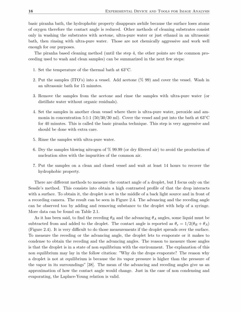
There are different methods to measure the contact angle of a droplet, but I focus only on the
Sessile’s method. This consists into obtain a high contrasted profile of that the drop interacts
with a surface. To obtain it, the droplet is set in the middle of a back light source and in front of
a recording camera. The result can be seen in Figure 2.4. The advancing and the receding angle
can be observed too by adding and removing substance to the droplet with help of a syringe.
More data can be found on Table 2.1.
As it has been said, to find the receding θR and the advancing θA angles, some liquid must be
subtracted from and added to the droplet. The contact angle is reported as θs = 1/2(θR + θA)
(Figure 2.4). It is very difficult to do those measurements if the droplet spreads over the surface.
To measure the receding or the advancing angle, the droplet lets to evaporate or it makes to
condense to obtain the receding and the advancing angles. The reason to measure those angles
is that the droplet is in a state of non equilibrium with the environment. The explanation of this
non equilibrium may lay in the follow citation: ”Why do the drops evaporate? The reason why
a droplet is not at equilibrium is because the its vapor pressure is higher than the pressure of
the vapor in its surroundings” [38]. The mean of the advancing and receding angles give us an
approximation of how the contact angle would change. Just in the case of non condensing and
evaporating, the Laplace-Young relation is valid.
Section 2.2 17
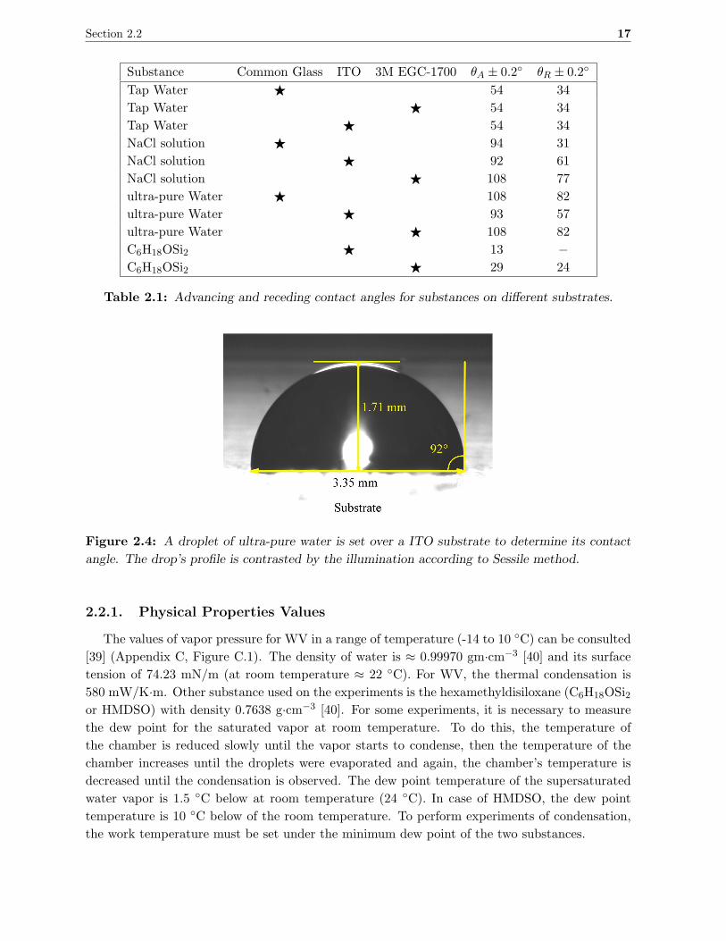
Substance Common Glass ITO 3M EGC-1700 θA ± 0.2 θR ± 0.2
Tap Water ⋆ 54 34
Tap Water ⋆ 54 34
Tap Water ⋆ 54 34
NaCl solution ⋆ 94 31
NaCl solution ⋆ 92 61
NaCl solution ⋆ 108 77
ultra-pure Water ⋆ 108 82
ultra-pure Water ⋆ 93 57
ultra-pure Water ⋆ 108 82
C6H18OSi2 ⋆ 13 −
C6H18OSi2 ⋆ 29 24
Table 2.1: Advancing and receding contact angles for substances on different substrates.
Figure 2.4: A droplet of ultra-pure water is set over a ITO substrate to determine its contact
angle. The drop’s profile is contrasted by the illumination according to Sessile method.
2.2.1. Physical Properties Values
The values of vapor pressure for WV in a range of temperature (-14 to 10 C) can be consulted
[39] (Appendix C, Figure C.1). The density of water is ≈ 0.99970 gm·cm−3 [40] and its surface
tension of 74.23 mN/m (at room temperature ≈ 22 C). For WV, the thermal condensation is
580 mW/K·m. Other substance used on the experiments is the hexamethyldisiloxane (C6H18OSi2or HMDSO) with density 0.7638 g·cm−3 [40]. For some experiments, it is necessary to measure
the dew point for the saturated vapor at room temperature. To do this, the temperature of
the chamber is reduced slowly until the vapor starts to condense, then the temperature of the
chamber increases until the droplets were evaporated and again, the chamber’s temperature is
decreased until the condensation is observed. The dew point temperature of the supersaturated
water vapor is 1.5 C below at room temperature (24 C). In case of HMDSO, the dew point
temperature is 10 C below of the room temperature. To perform experiments of condensation,
the work temperature must be set under the minimum dew point of the two substances.
18 Experimental Device and Tools for Image Analysis
2.3. Tools for Image Analysis
Image analysis is an important tool for this work. Frequently, it is found in the literature that
only simulation works offer many data to depict this kind of systems and about the experimental
work, only few reports can depict very well the evolution profile of complex systems. Some
calculus operations can be performed using routines for Matlab (mostly) from the data obtained.
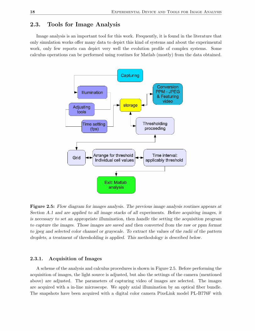
Figure 2.5: Flow diagram for images analysis. The previous image analysis routines appears at
Section A.1 and are applied to all image stacks of all experiments. Before acquiring images, it
is necessary to set an appropriate illumination, then handle the setting the acquisition program
to capture the images. Those images are saved and then converted from the raw or ppm format
to jpeg and selected color channel or grayscale. To extract the values of the radii of the pattern
droplets, a treatment of thresholding is applied. This methodology is described below.
2.3.1. Acquisition of Images
A scheme of the analysis and calculus procedures is shown in Figure 2.5. Before performing the
acquisition of images, the light source is adjusted, but also the settings of the camera (mentioned
above) are adjusted. The parameters of capturing video of images are selected. The images
are acquired with a in-line microscope. We apply axial illumination by an optical fiber bundle.
The snapshots have been acquired with a digital color camera PixeLink model PL-B776F with
Section 2.3 19
variable resolution from 800×600 to 2048×1536 pixels. The camera is mounted at the end of
the optics system of the microscope. The recording of images is done by a free Linux software
”Coriander”. The previous analysis starts with routines of ”FFmpeg” in order to separate colors,
modify formats (ppm to jpg, or others), or transform the stack of images from color to grayscale.
This Linux command is used to make videos of the experiments. The acquisition rate can variate
from 0.1 to 1 Hz depending on each experiment. depending on each experiment. In some cases
is desirable to use a high speed camera with a rate of 1000 fps for short times to observe certain
phenomena. In Appendix A a compendium of programs related with the image analysis can be
found.
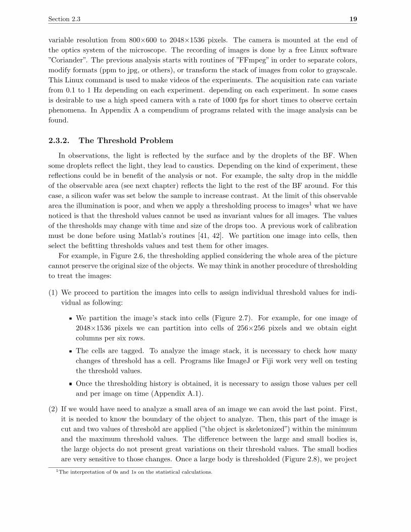
2.3.2. The Threshold Problem
In observations, the light is reflected by the surface and by the droplets of the BF. When
some droplets reflect the light, they lead to caustics. Depending on the kind of experiment, these
reflections could be in benefit of the analysis or not. For example, the salty drop in the middle
of the observable area (see next chapter) reflects the light to the rest of the BF around. For this
case, a silicon wafer was set below the sample to increase contrast. At the limit of this observable
area the illumination is poor, and when we apply a thresholding process to images1 what we have
noticed is that the threshold values cannot be used as invariant values for all images. The values
of the thresholds may change with time and size of the drops too. A previous work of calibration
must be done before using Matlab’s routines [41, 42]. We partition one image into cells, then
select the befitting thresholds values and test them for other images.
For example, in Figure 2.6, the thresholding applied considering the whole area of the picture
cannot preserve the original size of the objects. We may think in another procedure of thresholding
to treat the images:
(1) We proceed to partition the images into cells to assign individual threshold values for indi-
vidual as following:
We partition the image’s stack into cells (Figure 2.7). For example, for one image of
2048×1536 pixels we can partition into cells of 256×256 pixels and we obtain eight
columns per six rows.
The cells are tagged. To analyze the image stack, it is necessary to check how many
changes of threshold has a cell. Programs like ImageJ or Fiji work very well on testing
the threshold values.
Once the thresholding history is obtained, it is necessary to assign those values per cell
and per image on time (Appendix A.1).
(2) If we would have need to analyze a small area of an image we can avoid the last point. First,
it is needed to know the boundary of the object to analyze. Then, this part of the image is
cut and two values of threshold are applied (”the object is skeletonized”) within the minimum
and the maximum threshold values. The difference between the large and small bodies is,
the large objects do not present great variations on their threshold values. The small bodies
are very sensitive to those changes. Once a large body is thresholded (Figure 2.8), we project
1The interpretation of 0s and 1s on the statistical calculations.
20 Experimental Device and Tools for Image Analysis
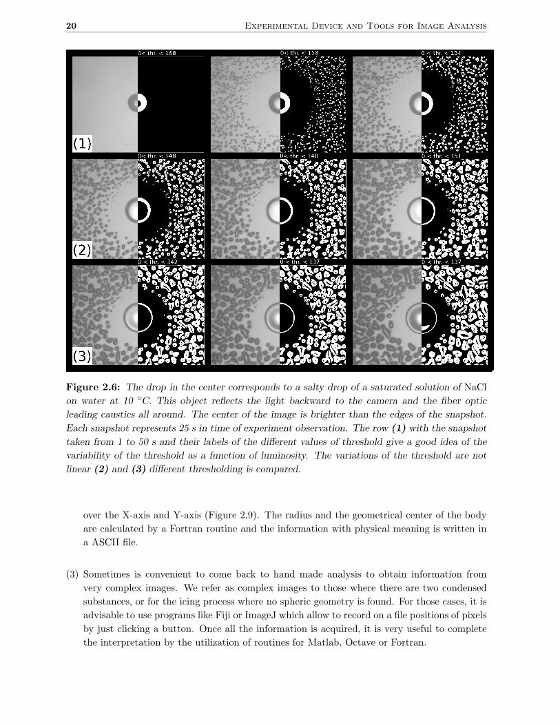
Figure 2.6: The drop in the center corresponds to a salty drop of a saturated solution of NaCl
on water at 10 C. This object reflects the light backward to the camera and the fiber optic
leading caustics all around. The center of the image is brighter than the edges of the snapshot.
Each snapshot represents 25 s in time of experiment observation. The row (1) with the snapshot
taken from 1 to 50 s and their labels of the different values of threshold give a good idea of the
variability of the threshold as a function of luminosity. The variations of the threshold are not
linear (2) and (3) different thresholding is compared.
over the X-axis and Y-axis (Figure 2.9). The radius and the geometrical center of the body
are calculated by a Fortran routine and the information with physical meaning is written in
a ASCII file.
(3) Sometimes is convenient to come back to hand made analysis to obtain information from
very complex images. We refer as complex images to those where there are two condensed
substances, or for the icing process where no spheric geometry is found. For those cases, it is
advisable to use programs like Fiji or ImageJ which allow to record on a file positions of pixels
by just clicking a button. Once all the information is acquired, it is very useful to complete
the interpretation by the utilization of routines for Matlab, Octave or Fortran.
Section 2.4 21
(4) In depth, for amorphous objects, instead of marking the edges of the objects in the picture,
it works very well to draw masks over them. The thresholding process is accurate during the
calculation of the areas and the counting the number of objects. The limitation is, the work
area is reduced and that the time spent drawing masks takes long time. This procedure is
applicable when it detected a special interesting area.
There are no straightforward measurements or/and computation of geometric amounts of the
droplets in the image stacks. Apparently, the method to choose depends on what part of the
system is sought after to apply one or other procedure of information extraction. The manual
methods rather than automatic processes are preferable when the shape of objects in the pattern
are not clearly defined. Otherwise, the automatic processes are good options when the analysis
of the objects in the pattern have geometric symmetries. For this last option, it must be done a
short previous procedure of preparation. In principle, it is necessary to choose the region where
the object is, and to know what maximum size it reaches. That means, to observe the maximum
time its size and to choose the limits to cut the image and reduce the image complexity. Before the
thresholding, it is possible to apply filters of fast Fourier transformations (FFT) too. Concerning
the measurements of the droplets of the BF, it is important to remark that not all the experiments
are candidates to apply an automatic analysis. Just few experiments can be treated with the cell
thresholding assignment. The option for those systems is the usage of a graphic tablet with a
digital stylus to mark the coordinates of the ends of the droplets, or to draw masks. After that,
it is recommended to run programs over the results to find the radii and other geometric values.
A very good example of the automatic image analysis is the BF in presence of a salty drop.
2.4. Errors
The different methodologies explained above have advantages and drawbacks. The procedures
for complex2 measurements can increase the error propagation. As it is mentioned before, it is
not desirable that the data have too much dispersion. Also it is suitable to have a balance among
the uncertain and the amount of data. In this section, I show a very basic protocol to compute
uncertainties for measurements obtained by programming in Matlab and ImageJ. With GNU
programs like Gimp, the maximum aspect of resolution for an image of 1536×2048 pixels. Taking
into account that this is the maximum the camera pixeLink’s resolution. At this respect, if we
use a microscope objective of 2X, the maximum size observable is ≈ 10 µm, which corresponds
to ≈ 4.65 pixels for clearest observation3 . The possibility that is left, is to consider an initial
error due to the noise and other non controllable factors during the experiments. We consider the
uncertainty is in a range of admissibility from 20 to 10 % of the mean area of the objects. The error
associated to the Matlab’s analysis comes from the process of binary thresholding. The selection
of thresholds values to represent a binary image are compared always with the size of objects
measured directly from original images. This measurement has assigned a ≈10 % as the error of
the appreciation of the bodies. Figure 2.8 shows the values of droplet radius (Figure 2.8) obtained
at different values of the threshold. The measured value of the central drop’s radius is 213±21.3
pixels or 459±45.9 µm. The value reported (the program is in Section 2) is 213.25±38 pixels,
2With many intermediate steps.3When the light contrasts, illumination, in the range of camera’s work temperature ,etc. are optimal.
22 Experimental Device and Tools for Image Analysis
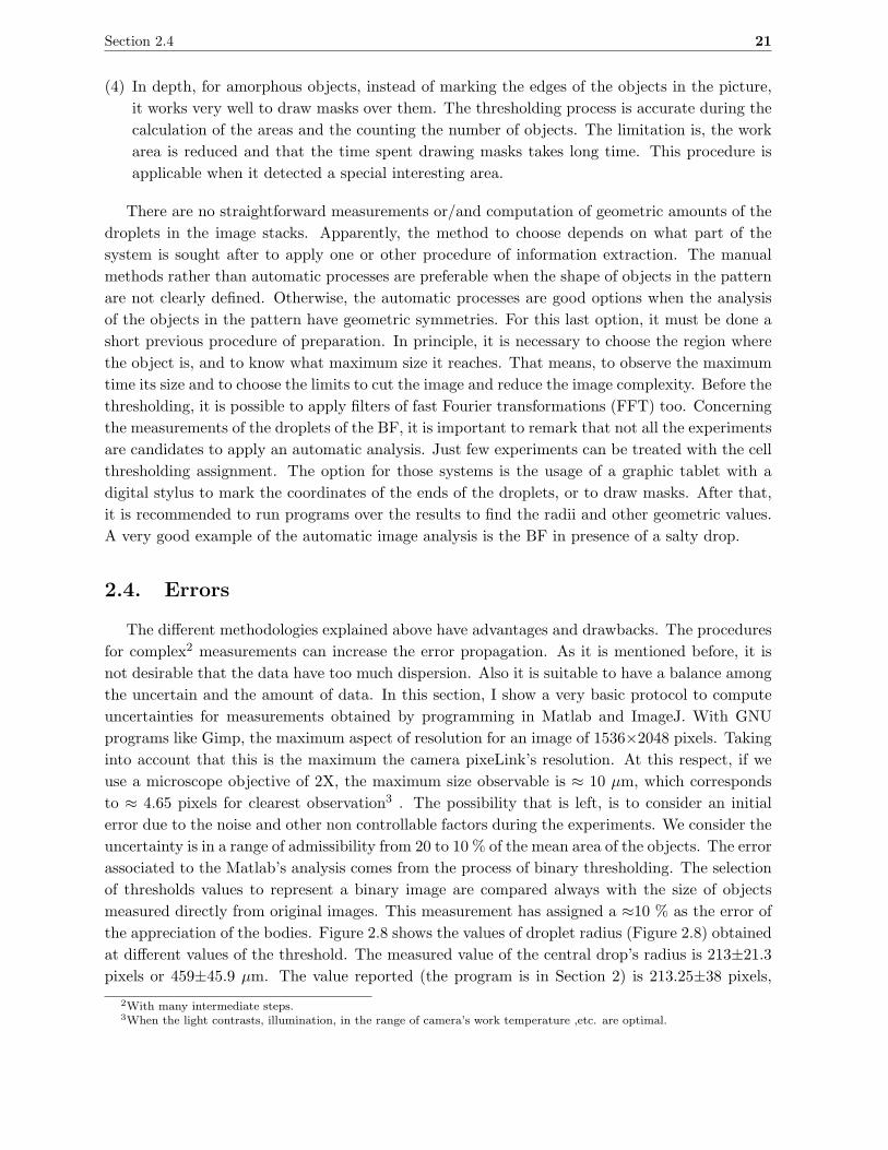
Figure 2.7: The snapshots have been partitioned and a thresholding has been applied according
to the methodological analysis described above. The change of the threshold value depends on
the position and the size of the droplets. The threshold is defined between upper and lower limits
to not blur the objects and preserve the number of droplets per cell. For this example, we refer
to the salty drop experiment. The corresponding series time of the experiment is: (a) to the time
t = 30 s, (b) to t = 250 s, (c) to t = 500 s and (d) to t = 900 s.
the interval where the peak has also and uncertainty, then is necessary to add the 10 % to the
uncertainty, thus 213.25±42 or 459±90 µm. In case of this example, the threshold value is 130
(Figure 2.9).
The uncertain associated with the Matlab’s analysis come from the process of binary thresh-
olding. The selection of thresholds values to represent a binary image are compared always with
the size of objects measured directly from original images. This measurement has assigned a
≈10 % as the uncertainty of the appreciation of the bodies. Figure 2.10 shows the values of
droplet radius (Figure 2.8) obtained at different values of the threshold. The measured value of
the central drop’s radius is 213±21.3 pixels or 459±45.9 µm. The value reported (the program
is in Section 2) is 213.25±38 pixels, the interval where the peak has also and uncertainty, then
is necessary to add the 10% to the uncertainty, thus 213.25±42 or 459±90 µm. In case of this
Section 2.4 23
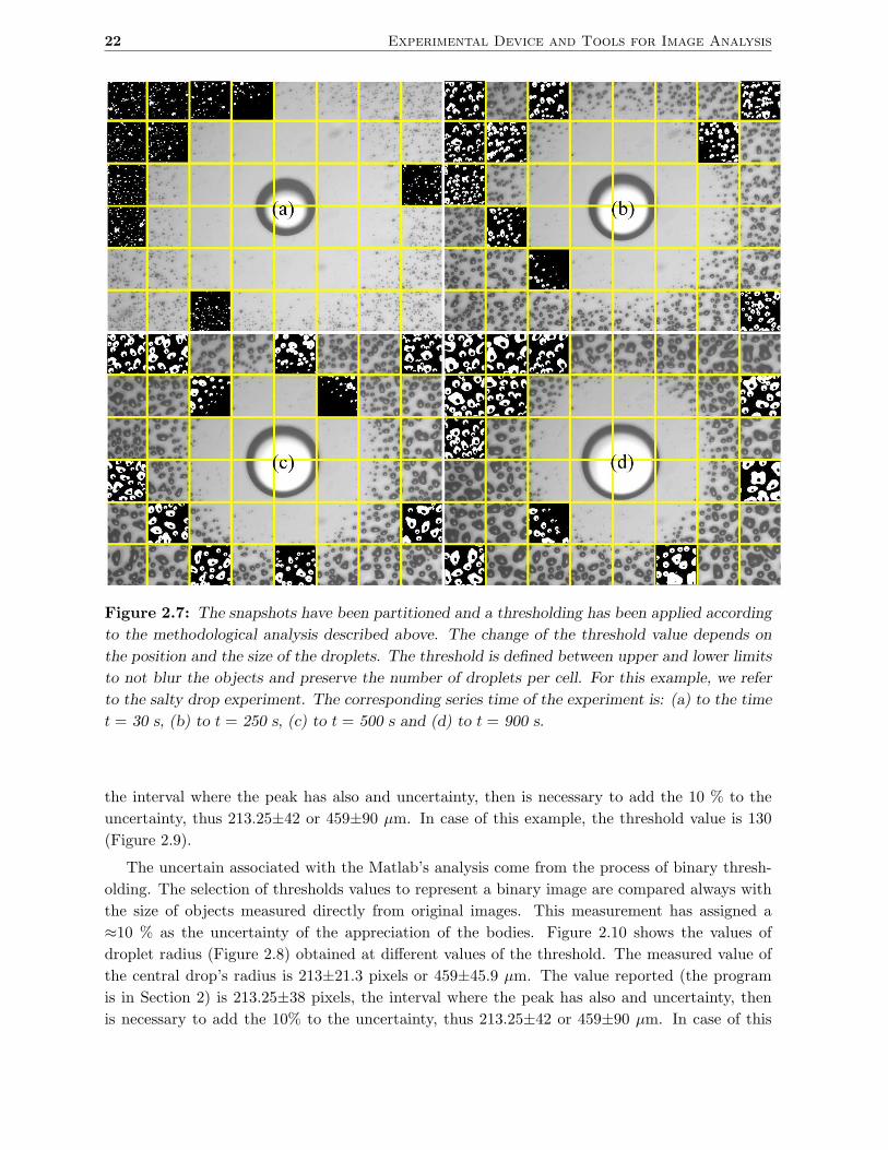
Figure 2.8: Different thresholding (from 40 and with an increment of 10 until 240, from left
to right) has been applied to the same image in order to describe how to find the proper value
threshold. The central drop is chosen as an example for uncertainty calculation.
Figure 2.9: (a) The projection’s droplet in horizontal orientation. (b) The projection on vertical
orientation. The limit of the central drop (for example) is chosen by applying different thresh-
olding. Then they are compared with the measure obtained from the original image. The entire
images with the threshold application are shown in Figure 2.8.
example, the threshold value is 130 (Figure 2.9).
24 Experimental Device and Tools for Image Analysis
50 100 150 200 250Threshold
140
160
180
200
220
240
R (
pixe
l)Threshold=130
R=213.25Ryreal
=211
Rxreal
=215.5
Rx
Ry
<R>
Matlab
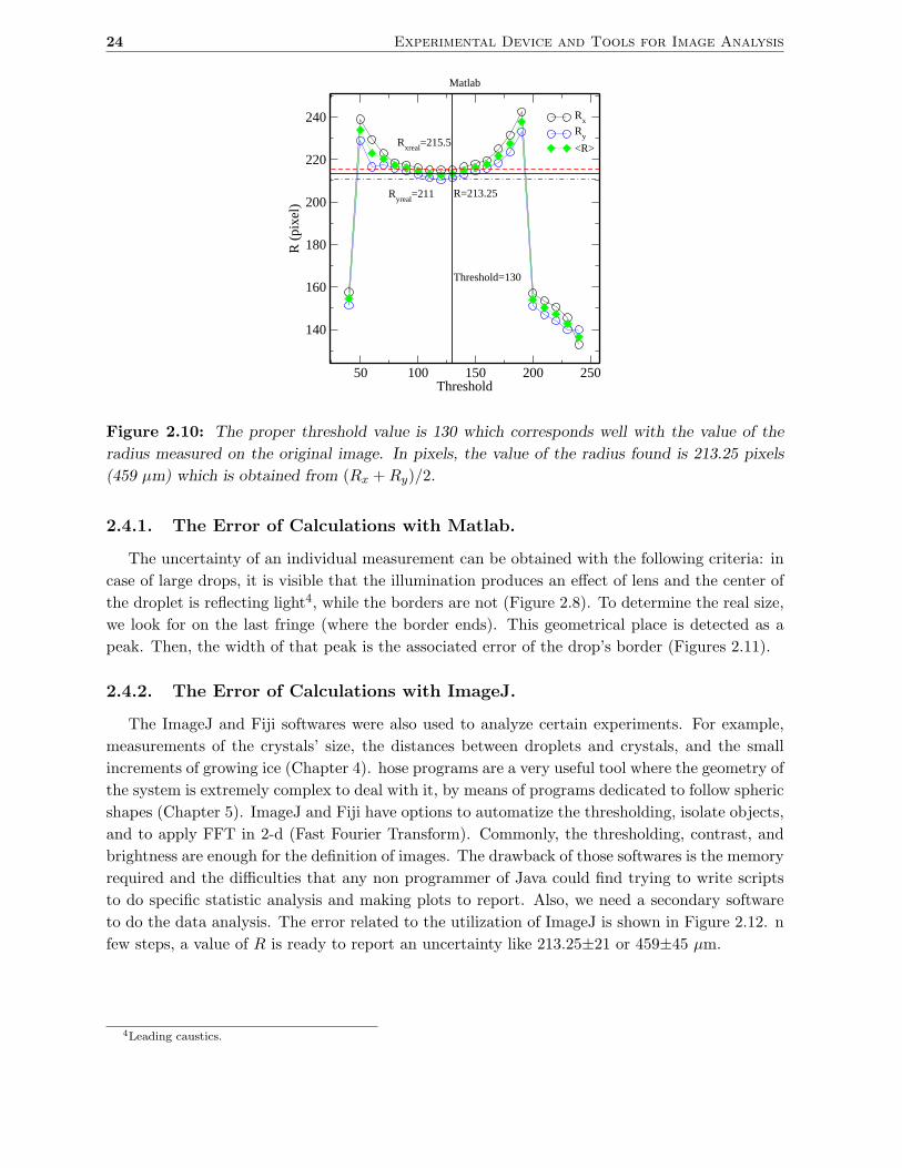
Figure 2.10: The proper threshold value is 130 which corresponds well with the value of the
radius measured on the original image. In pixels, the value of the radius found is 213.25 pixels
(459 µm) which is obtained from (Rx +Ry)/2.
2.4.1. The Error of Calculations with Matlab.
The uncertainty of an individual measurement can be obtained with the following criteria: in
case of large drops, it is visible that the illumination produces an effect of lens and the center of
the droplet is reflecting light4, while the borders are not (Figure 2.8). To determine the real size,
we look for on the last fringe (where the border ends). This geometrical place is detected as a
peak. Then, the width of that peak is the associated error of the drop’s border (Figures 2.11).
2.4.2. The Error of Calculations with ImageJ.
The ImageJ and Fiji softwares were also used to analyze certain experiments. For example,
measurements of the crystals’ size, the distances between droplets and crystals, and the small
increments of growing ice (Chapter 4). hose programs are a very useful tool where the geometry of
the system is extremely complex to deal with it, by means of programs dedicated to follow spheric
shapes (Chapter 5). ImageJ and Fiji have options to automatize the thresholding, isolate objects,
and to apply FFT in 2-d (Fast Fourier Transform). Commonly, the thresholding, contrast, and
brightness are enough for the definition of images. The drawback of those softwares is the memory
required and the difficulties that any non programmer of Java could find trying to write scripts
to do specific statistic analysis and making plots to report. Also, we need a secondary software
to do the data analysis. The error related to the utilization of ImageJ is shown in Figure 2.12. n
few steps, a value of R is ready to report an uncertainty like 213.25±21 or 459±45 µm.
4Leading caustics.
Section 2.4 25
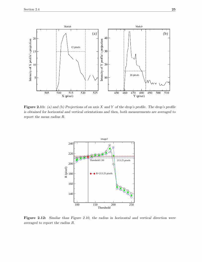
Figure 2.11: (a) and (b) Projections of on axis X and Y of the drop’s profile. The drop’s profile
is obtained for horizontal and vertical orientations and then, both measurements are averaged to
report the mean radius R.
100 150 200 250Threshold
140
160
180
200
220
240
R (
pixe
l)
213.25 pixels
R=213.25 pixels
imageJ
Threshold 130
Figure 2.12: Similar than Figure 2.10, the radius in horizontal and vertical direction were
averaged to report the radius R.

26 Experimental Device and Tools for Image Analysis
Chapter 3
Breath Figures in Presence of a
Humidity Sink
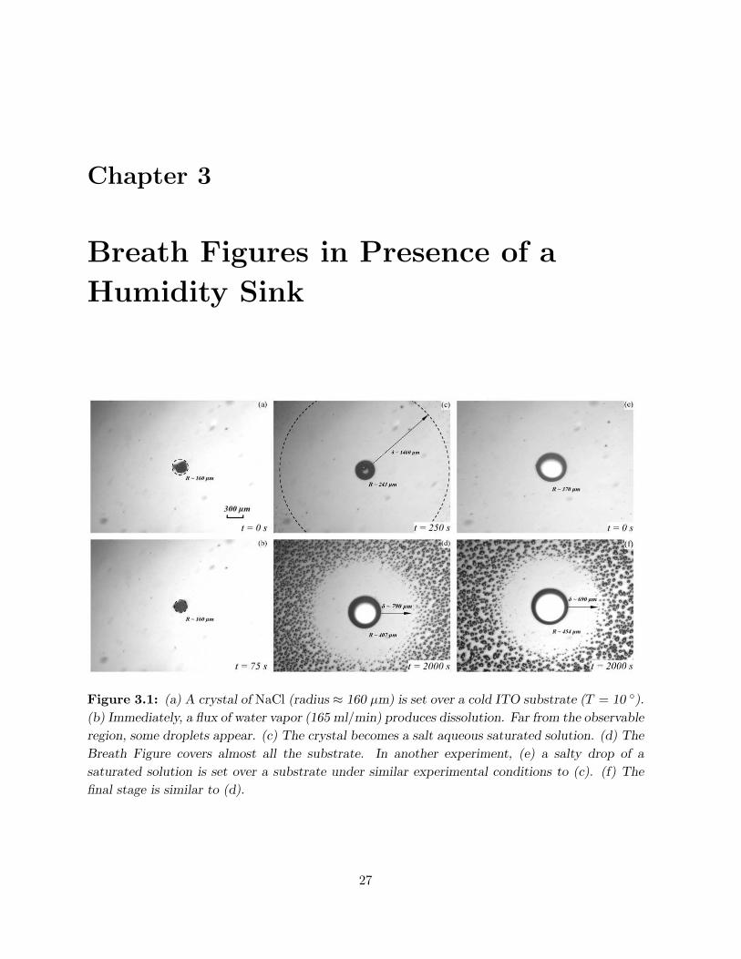
Figure 3.1: (a) A crystal of NaCl (radius ≈ 160 µm) is set over a cold ITO substrate (T = 10 ).
(b) Immediately, a flux of water vapor (165 ml/min) produces dissolution. Far from the observable
region, some droplets appear. (c) The crystal becomes a salt aqueous saturated solution. (d) The
Breath Figure covers almost all the substrate. In another experiment, (e) a salty drop of a
saturated solution is set over a substrate under similar experimental conditions to (c). (f) The
final stage is similar to (d).
27
28 Breath Figures in Presence of a Humidity Sink
3.1. Introduction
For the life in general, water is very important. In many processes water plays the main role in
life of human beings, animals and plants. Water on Earth is interconnected with the atmosphere,
oceans, aquifers by hydrological cycles. From global point of view, the water resources and
the recollection are becoming a matter of strategy to supply of national security in developed
countries. So the studies of water properties should have priority.
At physical chemistry level, when water plays the role of solvent or catalyst, it may modify
the thermal and chemical properties of the substances. The aim of this chapter is to understand
the BF formation process in presence of a humidity sink. The physical chemistry problem is
studied from the point of view of the dynamics where the volume change on time as water is
added to the salt crystal by WV condensation. Once the salt solution has reached a certain
water concentration, the BF is visible (on the observable area) and the average size of the water
droplets can be measured at certain distance of the salty drop. This information can be used
as an indicator of the values of the partial pressures distributed around to the humidity sink, as
well, the amount of water condensed. The research on the interaction of WV with a salty drop
started by J. S. Owens in 1922 [43]. Some decades, R. Williams and J. Blanc [44] have attempted
to explain what it is the influence on the surrounding of a crystal collecting WV. The subject of
the study it is a NaCl crystal in presence of condensing WV. They argued that the temperature
is the main variable and it could be related with the difference of pressures of supersaturated
WV. However, they have not offered a description of the entire process of condensation evolution.
Furthermore, C. Schafle, et al. [45] have said the BF formation is due just to a heterogeneous
nucleation without deep in the analysis and just by the examination the depletion zone of an
arrangement of sinks.
The initial idea of this research work is due to Dr. Ramchandra Narhe in 2007. He suggested
an experiment to create a concentration gradient by setting a humidity sink on a BF like a salt
crystal. The very well known growth laws of BF are used to understand the evolution of the system
in this configuration. The sink used to perform the experiments (Figure 3.1) is a NaCl+H2O salt
solution in a hemispheric droplet shape. The sink capacity to adsorb vapor will decrease as a
function of time, while the depleted zone between the BF will shrink. All the challenges have
come when we have tried to extract information from the visualizations. At the beginning of this
research, we have done the experiments to follow in time the BF formation and simultaneously
the salty drop evolution. That meant, the objective of the microscope was moved in all directions
trying to scan parts of the salty drop, parts of the depletion zone, and the drop’s carpet. The
first difficulty of this methodology was to match the images at different positions and at different
times. So, we have decided to set over the substrate a very small salty drop to observe the three
regions of the system. At that time, this resulted a very good idea but in practice was not so easy,
because not very small drops could be obtained using syringes and micropipets. The constant
problem has still been the size of the salty drop. To have control on the micro scale was not so
easy as we have thought. We have found that the way to set a small salty drop was to put a
drop on the substrate, then evaporate it and separate the small crystals with a needle. Once a
small crystal has been separated, a drop was obtained again by the humidity and because the
temperature of the substrate was decreased. After this, it was necessary to pay attention at the
Section 3.2 29
water vapor source. As a reservoir of vapor we have used a wet cloth. It resulted a not very
stable source as humidity decreased upon time. The solution to this was to install a pump to flow
N2 (or dry filtered air) through a flask bubbling ultra-pure water. The other improvement was
to install a temperature controller to avoid high variations of the temperature. Once all those
improvements have been applied, we noticed that we have not had any reference of what should
be the amount of salt on the solution. We prepared a salt saturated solution at T = 10C. Now,
finally the ideas of how to perform this experiment were completed, it was left improve the image
data processing. A lot of time we have spent in writing code, testing it and comparing the results.
The first difference between the old perspective and the new is, that with the new procedures we
could reduce the data dispersion and increase the time resolution. Now, we could do conjecture
about the phenomenon like the physical reference mentioned above. The exactly moment when
the crystal salt is totally dissolved is the time and radius reference. At this time, the salty drop
reaches the condition of saturated solution at the operation temperature. We have found that
the growth law of the salty drop depends on this value. The depletion zone evolution can be
explained using those references. We will see that the radius and time are useful to obtain the
partial pressures at the perimeter of the salty drop, on the depletion zone and where it ends.
How the vapor concentration is distributed around the salty drop is also a question to solve
in this work. The physical process of ”Breath Figure in presence of a humidity sink” has begun
to be observed with more detail. We have developed a methodology to do measurements and to
gather accurate information. At the same time, other questions have arisen from the calculations
like for example which could be a suitable analysis to understand the WV concentration and to
describe the system. This question has driven the analysis of 〈r〉 as a function of time t and an
area defined on the rings zone R+δ < d < δ+∆δ where ∆δ is the maximum value of the diameter
of a droplet in the BF and d is the width of the ring. Other question arised like: What are the
best spatial contour to compute 〈r〉t to give the best and realistic depiction of the BF? Other
questions have emerged too. What is the relation between R and δ? and, what is the difference
of pressures between the salty drop perimeter and the beginning of the BF? I will deal with these
questions in the next sections.
3.2. Experimental Procedure
The description of these series of experiments is based on the Chapter 2. The ITO was
chosen for the experiments and two possibilities to set the salty over the substrate were done: a
submilimeter salty drop is set over the substrate to do the experiment. Previously, it was made
a salt solution (for 10 C, the proportion of NaCl is 35.72 g on 100 g of water [40]). The other
procedure consists into set a salty drop, evaporate it by heating the substrate, spread the small
crystals, and focus the microscope over the smallest crystal, set the temperature at 10 C and flow
the water vapor. Both cases are very similar and the results are comparable (Figure 3.1). The
first methodology is easy to follow but the salty drop set over the substrate cannot be controlled
properly and during the observations the time reference and initial radius are missed. With the
second methodology, the references can be set. There is another benefit in the latter method.
It is easy to recognize the time where the crystal salt is dissolved and in consequence, the exact
time where the salty drop reaches the saturated condition.
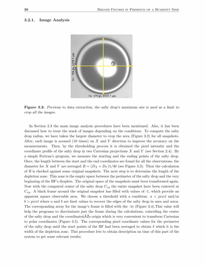
30 Breath Figures in Presence of a Humidity Sink
3.2.1. Image Analysis
Figure 3.2: Previous to data extraction, the salty drop’s maximum size is used as a limit to
crop all the images.
In Section 2.3 the main image analysis procedures have been mentioned. Also, it has been
discussed how to treat the stack of images depending on the conditions. To compute the salty
drop radius, we have taken the largest diameter to crop the area (Figure 3.2) for all snapshots.
After, each image is zoomed (10 times) on X and Y direction to improve the accuracy on the
measurements. Then, by the thresholding process it is obtained the pixel intensity and the
coordinate profile of the salty drop in two Cartesian projections X and Y (see Section 2.4). By
a simple Fortran’s program, we measure the starting and the ending points of the salty drop.
Once, the length between the start and the end coordinates are found for all the observations, the
diameter for X and Y are averaged R = (DX +DY )1/40 (see Figure 3.3). Then the calculation
of R is checked against some original snapshots. The next step is to determine the length of the
depletion zone. This zone is the empty space between the perimeter of the salty drop and the very
beginning of the BF’s droplets. The original space of the snapshots must been transformed again.
Now with the computed center of the salty drop Cxy the entire snapshot have been centered at
Cxy. A black frame around the original snapshot has filled with values of -1, which provide an
apparent square observable area. We choose a threshold with a condition: a < pixel and/or
b > pixel where a and b are limit values to recover the edges of the salty drop in ones and zeros.
The corresponding array for the image’s frame is filled with the -1s (Figure 3.4).This value will
help the programs to discriminate just the frame during the calculations, coinciding the center
of the salty drop and the coordinateaAZs origin which is very convenient to transform Cartesian
to polar coordinates (Figure 3.5). The corresponding pixel coordinate values for the perimeter
of the salty drop until the start points of the BF had been averaged to obtain δ which it is the
width of the depletion zone. This procedure lets to obtain description on time of this part of the
system to get some relevant results.
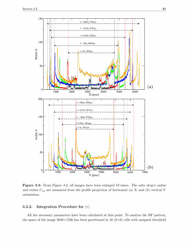
Section 3.2 31
Figure 3.3: From Figure 3.2, all images have been enlarged 10 times. The salty drop’s radius
and center Cxy are measured from the profile projection of horizontal (a) X and (b) vertical Y
orientation.
3.2.2. Integration Procedure for 〈r〉
All the necessary parameters have been calculated at this point. To analyze the BF pattern,
the space of the image 2048×1536 has been partitioned in 48 (8×6) cells with assigned threshold
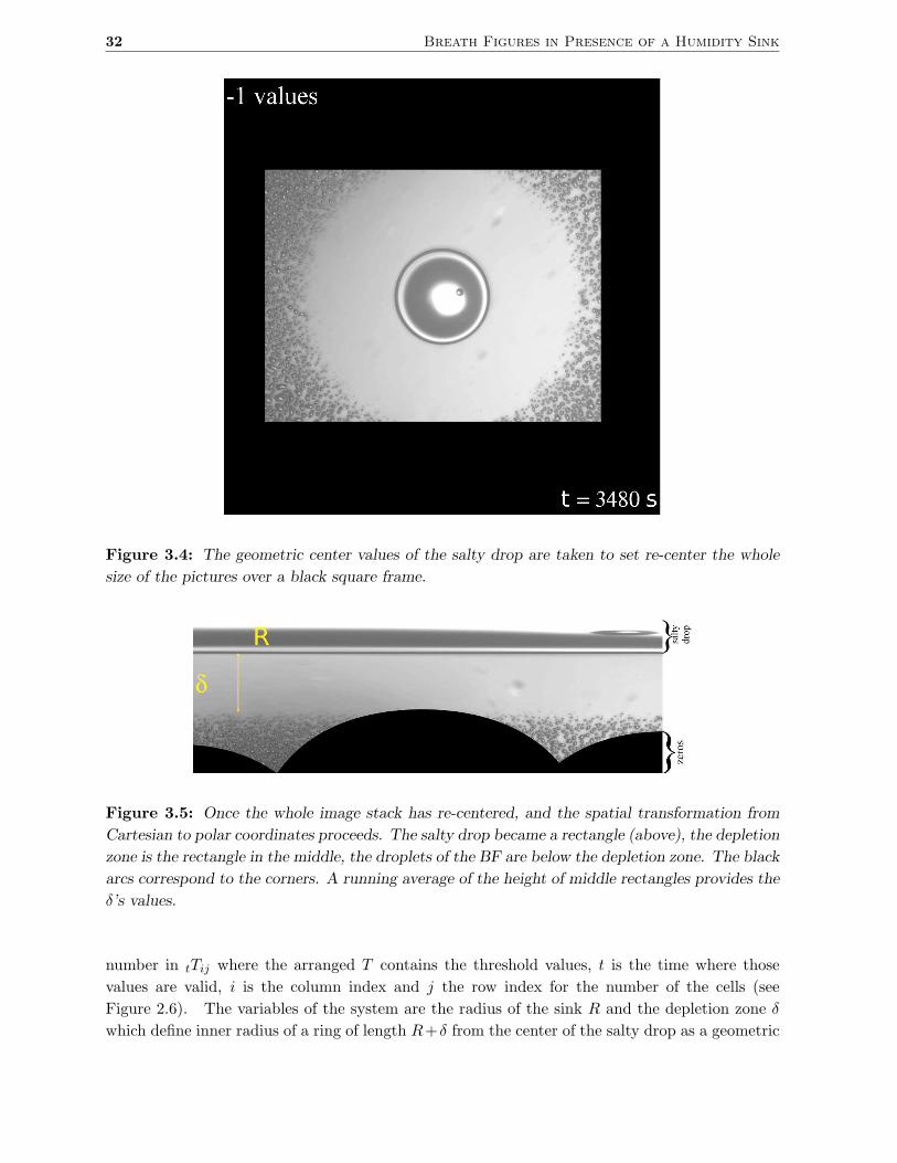
32 Breath Figures in Presence of a Humidity Sink
Figure 3.4: The geometric center values of the salty drop are taken to set re-center the whole
size of the pictures over a black square frame.
Figure 3.5: Once the whole image stack has re-centered, and the spatial transformation from
Cartesian to polar coordinates proceeds. The salty drop became a rectangle (above), the depletion
zone is the rectangle in the middle, the droplets of the BF are below the depletion zone. The black
arcs correspond to the corners. A running average of the height of middle rectangles provides the
δ’s values.
number in tTij where the arranged T contains the threshold values, t is the time where those
values are valid, i is the column index and j the row index for the number of the cells (see
Figure 2.6). The variables of the system are the radius of the sink R and the depletion zone δ
which define inner radius of a ring of length R+δ from the center of the salty drop as a geometric
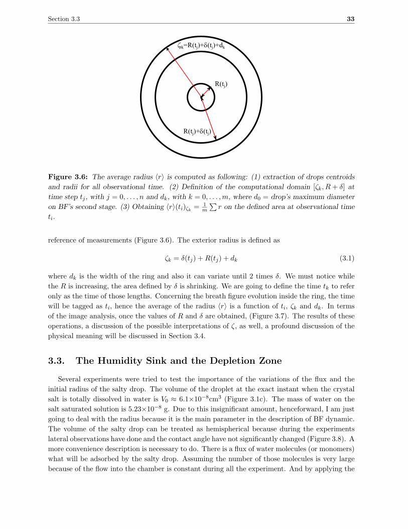
Section 3.3 33
Figure 3.6: The average radius 〈r〉 is computed as following: (1) extraction of drops centroids
and radii for all observational time. (2) Definition of the computational domain [ζk, R+ δ] at
time step tj , with j = 0, . . . , n and dk, with k = 0, . . . ,m, where d0 = drop’s maximum diameter
on BF’s second stage. (3) Obtaining 〈r〉(ti)ζk = 1m
∑
r on the defined area at observational time
ti.
reference of measurements (Figure 3.6). The exterior radius is defined as
ζk = δ(tj) +R(tj) + dk (3.1)
where dk is the width of the ring and also it can variate until 2 times δ. We must notice while
the R is increasing, the area defined by δ is shrinking. We are going to define the time tk to refer
only as the time of those lengths. Concerning the breath figure evolution inside the ring, the time
will be tagged as ti, hence the average of the radius 〈r〉 is a function of ti, ζk and dk. In terms
of the image analysis, once the values of R and δ are obtained, (Figure 3.7). The results of these
operations, a discussion of the possible interpretations of ζ, as well, a profound discussion of the
physical meaning will be discussed in Section 3.4.
3.3. The Humidity Sink and the Depletion Zone
Several experiments were tried to test the importance of the variations of the flux and the
initial radius of the salty drop. The volume of the droplet at the exact instant when the crystal
salt is totally dissolved in water is V0 ≈ 6.1×10⁻⁸cm3 (Figure 3.1c). The mass of water on the
salt saturated solution is 5.23×10⁻⁸ g. Due to this insignificant amount, henceforward, I am just
going to deal with the radius because it is the main parameter in the description of BF dynamic.
The volume of the salty drop can be treated as hemispherical because during the experiments
lateral observations have done and the contact angle have not significantly changed (Figure 3.8). A
more convenience description is necessary to do. There is a flux of water molecules (or monomers)
what will be adsorbed by the salty drop. Assuming the number of those molecules is very large
because of the flow into the chamber is constant during all the experiment. And by applying the
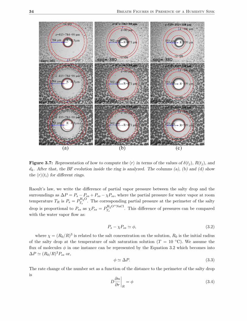
34 Breath Figures in Presence of a Humidity Sink
Figure 3.7: Representation of how to compute the 〈r〉 in terms of the values of δ(tj), R(tj), and
dk. After that, the BF evolution inside the ring is analyzed. The columns (a), (b) and (d) show
the 〈r〉(ti) for different rings.
Raoult’s law, we write the difference of partial vapor pressure between the salty drop and the
surroundings as ∆P = Ps −Pss +Pss −χPss, where the partial pressure for water vapor at room
temperature TR is Ps = PH
2O
Ts. The corresponding partial pressure at the perimeter of the salty
drop is proportional to Pss as χPss = PH
2O+NaCl
Ts. This difference of pressures can be compared
with the water vapor flow as:
Ps − χPss ≃ φ, (3.2)
where χ = (R0/R)3 is related to the salt concentration on the solution, R0 is the initial radius
of the salty drop at the temperature of salt saturation solution (T = 10 C). We assume the
flux of molecules φ in one instance can be represented by the Equation 3.2 which becomes into
∆P ≃ (R0/R)3Pss or,
φ ≃ ∆P. (3.3)
The rate change of the number set as a function of the distance to the perimeter of the salty drop
is
D∂n
∂r
∣
∣
∣
∣
R
= φ (3.4)
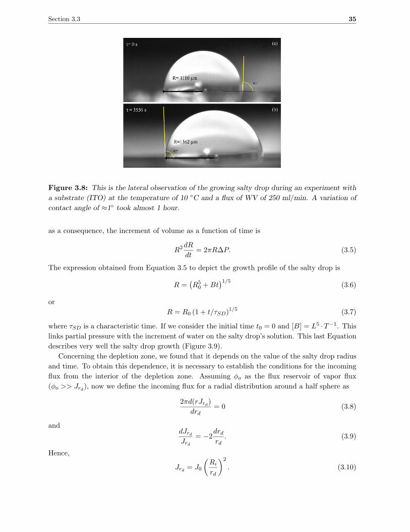
Section 3.3 35
Figure 3.8: This is the lateral observation of the growing salty drop during an experiment with
a substrate (ITO) at the temperature of 10 C and a flux of WV of 250 ml/min. A variation of
contact angle of ≈1 took almost 1 hour.
as a consequence, the increment of volume as a function of time is
R2 dR
dt= 2πR∆P. (3.5)
The expression obtained from Equation 3.5 to depict the growth profile of the salty drop is
R =(
R50 +Bt
)1/5(3.6)
or
R = R0 (1 + t/τSD)1/5 (3.7)
where τSD is a characteristic time. If we consider the initial time t0 = 0 and [B] = L5 ·T−1. This
links partial pressure with the increment of water on the salty drop’s solution. This last Equation
describes very well the salty drop growth (Figure 3.9).
Concerning the depletion zone, we found that it depends on the value of the salty drop radius
and time. To obtain this dependence, it is necessary to establish the conditions for the incoming
flux from the interior of the depletion zone. Assuming φo as the flux reservoir of vapor flux
(φo >> Jrd), now we define the incoming flux for a radial distribution around a half sphere as
2πd(rJrd)
drd= 0 (3.8)
anddJrdJrd
= −2drdrd
. (3.9)
Hence,
Jrd = J0
(
Ri
rd
)2
. (3.10)
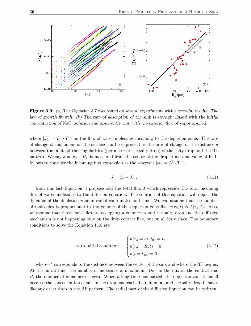
36 Breath Figures in Presence of a Humidity Sink
Figure 3.9: (a) The Equation 3.7 was tested on several experiments with successful results. The
law of growth fit well. (b) The rate of adsorption of the sink is strongly linked with the initial
concentration of NaCl solution and apparently, not with the exterior flux of vapor applied.
where [J0] = L3 · T−1 is the flux of water molecules incoming to the depletion zone. The rate
of change of monomers on the surface can be expressed as the rate of change of the distance δ
between the limits of the singularities (perimeter of the salty drop) of the salty drop and the BF
pattern. We say δ = |rd − Ri| is measured from the center of the droplet at some value of R. It
follows to consider the incoming flux expression as the reservoir [φo] = L3 · T−1.
J = φo − Jrd , (3.11)
from this last Equation, I propose add the total flux J which represents the total incoming
flux of water molecules to the diffusion equation. The solution of this equation will depict the
dynamic of the depletion zone in radial coordinates and time. We can assume that the number
of molecules is proportional to the volume of the depletion zone like n(rd, t) ∝ δ(rd, t). Also,
we assume that those molecules are occupying a volume around the salty drop and the diffusive
mechanism is not happening only on the drop contact line, but on all its surface. The boundary
conditions to solve the Equation 1.18 are
with initial conditions:
n(rd = r∗, t0) = n0
n(rd = R, t) = 0
n(t = t∞) = 0
(3.12)
where r∗ corresponds to the distance between the center of the sink and where the BF begins.
At the initial time, the number of molecules is maximum. Due to the flux at the contact line
R, the number of monomers is zero. When a long time has passed, the depletion zone is small
because the concentration of salt in the drop has reached a minimum, and the salty drop behaves
like any other drop in the BF pattern. The radial part of the diffusive Equation can be written
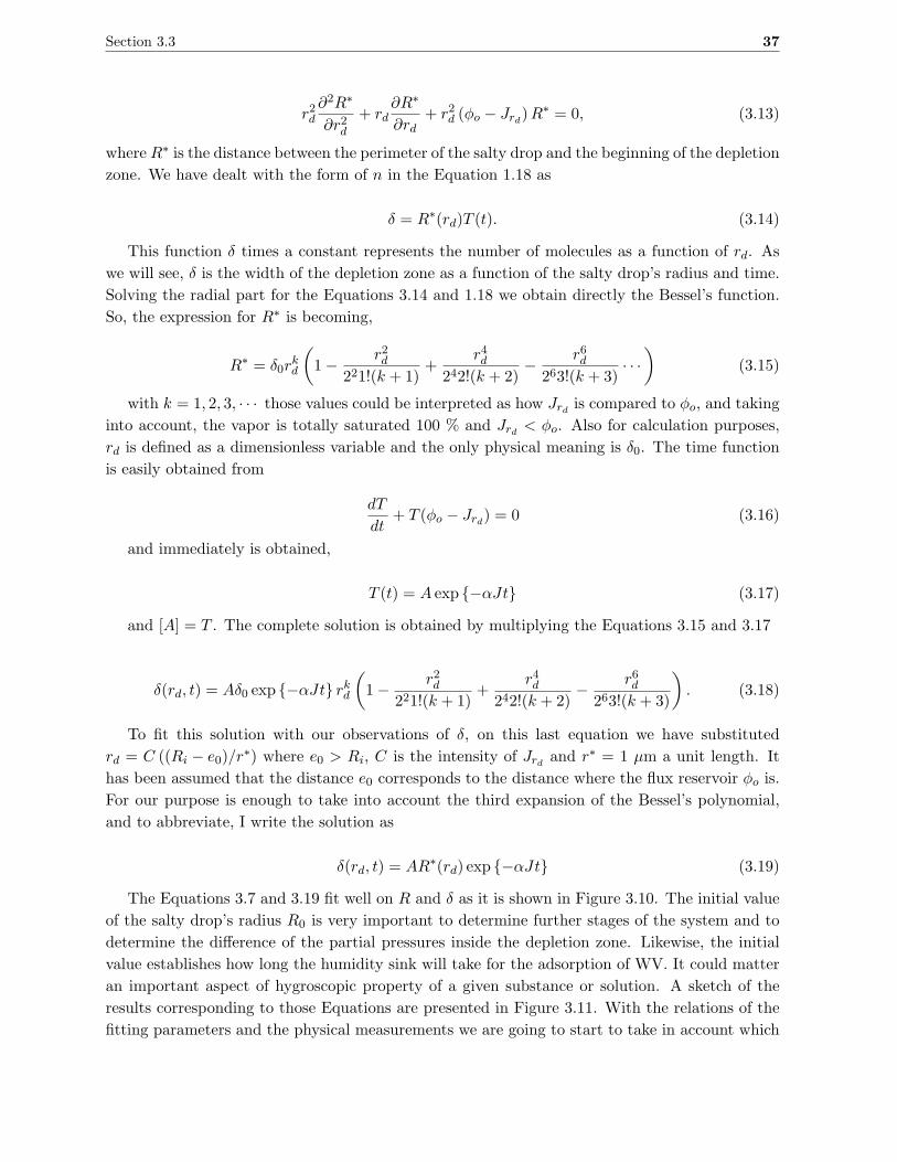
Section 3.3 37
r2d∂2R∗
∂r2d+ rd
∂R∗
∂rd+ r2d (φo − Jrd)R
∗ = 0, (3.13)
where R∗ is the distance between the perimeter of the salty drop and the beginning of the depletion
zone. We have dealt with the form of n in the Equation 1.18 as
δ = R∗(rd)T (t). (3.14)
This function δ times a constant represents the number of molecules as a function of rd. As
we will see, δ is the width of the depletion zone as a function of the salty drop’s radius and time.
Solving the radial part for the Equations 3.14 and 1.18 we obtain directly the Bessel’s function.
So, the expression for R∗ is becoming,
R∗ = δ0rkd
(
1−r2d
221!(k + 1)+
r4d242!(k + 2)
−r6d
263!(k + 3)· · ·
)
(3.15)
with k = 1, 2, 3, · · · those values could be interpreted as how Jrd is compared to φo, and taking
into account, the vapor is totally saturated 100 % and Jrd < φo. Also for calculation purposes,
rd is defined as a dimensionless variable and the only physical meaning is δ0. The time function
is easily obtained from
dT
dt+ T (φo − Jrd) = 0 (3.16)
and immediately is obtained,
T (t) = A exp −αJt (3.17)
and [A] = T . The complete solution is obtained by multiplying the Equations 3.15 and 3.17
δ(rd, t) = Aδ0 exp −αJt rkd
(
1−r2d
221!(k + 1)+
r4d242!(k + 2)
−r6d
263!(k + 3)
)
. (3.18)
To fit this solution with our observations of δ, on this last equation we have substituted
rd = C ((Ri − e0)/r∗) where e0 > Ri, C is the intensity of Jrd and r∗ = 1 µm a unit length. It
has been assumed that the distance e0 corresponds to the distance where the flux reservoir φo is.
For our purpose is enough to take into account the third expansion of the Bessel’s polynomial,
and to abbreviate, I write the solution as
δ(rd, t) = AR∗(rd) exp −αJt (3.19)
The Equations 3.7 and 3.19 fit well on R and δ as it is shown in Figure 3.10. The initial value
of the salty drop’s radius R0 is very important to determine further stages of the system and to
determine the difference of the partial pressures inside the depletion zone. Likewise, the initial
value establishes how long the humidity sink will take for the adsorption of WV. It could matter
an important aspect of hygroscopic property of a given substance or solution. A sketch of the
results corresponding to those Equations are presented in Figure 3.11. With the relations of the
fitting parameters and the physical measurements we are going to start to take in account which
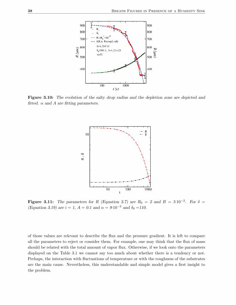
38 Breath Figures in Presence of a Humidity Sink
Figure 3.10: The evolution of the salty drop radius and the depletion zone are depicted and
fitted. α and A are fitting parameters.
Figure 3.11: The parameters for R (Equation 3.7) are R0 = 2 and B = 5·10−2. For δ =
(Equation 3.19) are i = 1, A = 0.1 and α = 9·10−3 and δ0 =110.
of those values are relevant to describe the flux and the pressure gradient. It is left to compare
all the parameters to reject or consider them. For example, one may think that the flux of mass
should be related with the total amount of vapor flux. Otherwise, if we look onto the parameters
displayed on the Table 3.1 we cannot say too much about whether there is a tendency or not.
Perhaps, the interaction with fluctuations of temperature or with the roughness of the substrates
are the main cause. Nevertheless, this understandable and simple model gives a first insight to
the problem.
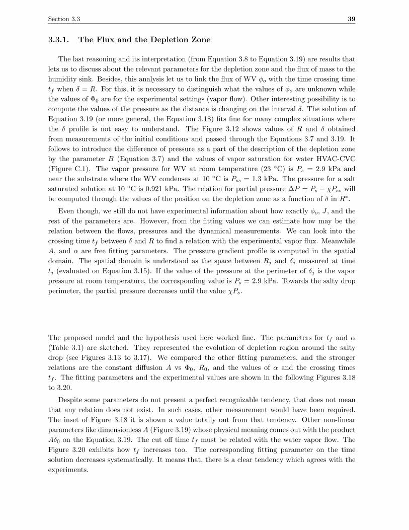
Section 3.3 39
3.3.1. The Flux and the Depletion Zone
The last reasoning and its interpretation (from Equation 3.8 to Equation 3.19) are results that
lets us to discuss about the relevant parameters for the depletion zone and the flux of mass to the
humidity sink. Besides, this analysis let us to link the flux of WV φo with the time crossing time
tf when δ = R. For this, it is necessary to distinguish what the values of φo are unknown while
the values of Φ0 are for the experimental settings (vapor flow). Other interesting possibility is to
compute the values of the pressure as the distance is changing on the interval δ. The solution of
Equation 3.19 (or more general, the Equation 3.18) fits fine for many complex situations where
the δ profile is not easy to understand. The Figure 3.12 shows values of R and δ obtained
from measurements of the initial conditions and passed through the Equations 3.7 and 3.19. It
follows to introduce the difference of pressure as a part of the description of the depletion zone
by the parameter B (Equation 3.7) and the values of vapor saturation for water HVAC-CVC
(Figure C.1). The vapor pressure for WV at room temperature (23 C) is Ps = 2.9 kPa and
near the substrate where the WV condenses at 10 C is Pss = 1.3 kPa. The pressure for a salt
saturated solution at 10 C is 0.921 kPa. The relation for partial pressure ∆P = Ps − χPss will
be computed through the values of the position on the depletion zone as a function of δ in R∗.
Even though, we still do not have experimental information about how exactly φo, J , and the
rest of the parameters are. However, from the fitting values we can estimate how may be the
relation between the flows, pressures and the dynamical measurements. We can look into the
crossing time tf between δ and R to find a relation with the experimental vapor flux. Meanwhile
A, and α are free fitting parameters. The pressure gradient profile is computed in the spatial
domain. The spatial domain is understood as the space between Rj and δj measured at time
tj (evaluated on Equation 3.15). If the value of the pressure at the perimeter of δj is the vapor
pressure at room temperature, the corresponding value is Ps = 2.9 kPa. Towards the salty drop
perimeter, the partial pressure decreases until the value χPs.
The proposed model and the hypothesis used here worked fine. The parameters for tf and α
(Table 3.1) are sketched. They represented the evolution of depletion region around the salty
drop (see Figures 3.13 to 3.17). We compared the other fitting parameters, and the stronger
relations are the constant diffusion A vs Φ0, R0, and the values of α and the crossing times
tf . The fitting parameters and the experimental values are shown in the following Figures 3.18
to 3.20.
Despite some parameters do not present a perfect recognizable tendency, that does not mean
that any relation does not exist. In such cases, other measurement would have been required.
The inset of Figure 3.18 it is shown a value totally out from that tendency. Other non-linear
parameters like dimensionless A (Figure 3.19) whose physical meaning comes out with the product
Aδ0 on the Equation 3.19. The cut off time tf must be related with the water vapor flow. The
Figure 3.20 exhibits how tf increases too. The corresponding fitting parameter on the time
solution decreases systematically. It means that, there is a clear tendency which agrees with the
experiments.
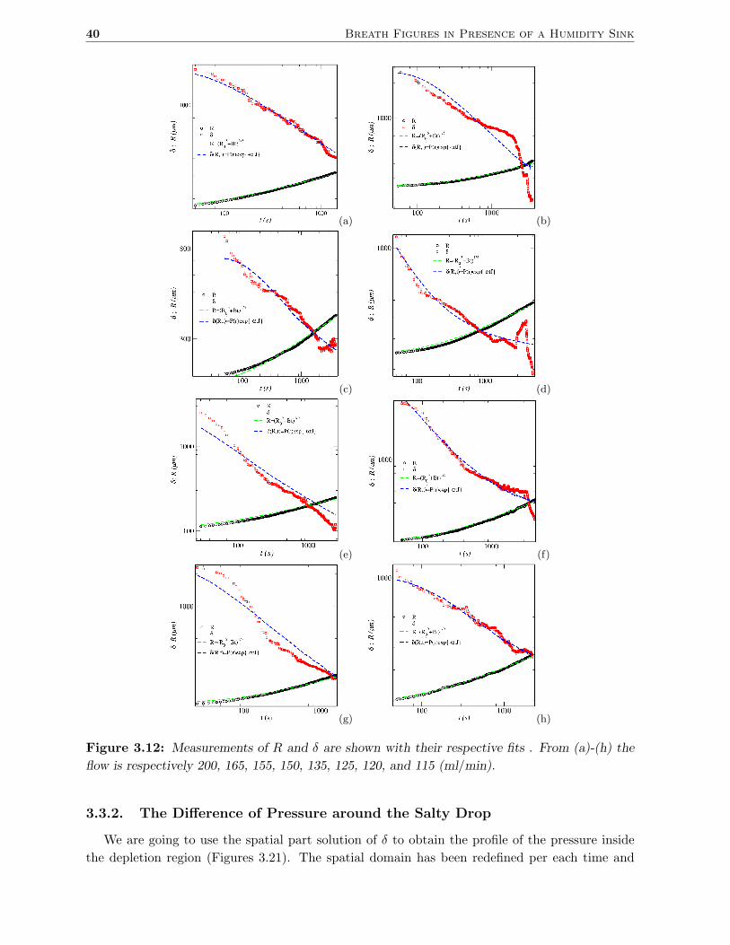
40 Breath Figures in Presence of a Humidity Sink
(a) (b)
(c) (d)
(e) (f)
(g) (h)
Figure 3.12: Measurements of R and δ are shown with their respective fits . From (a)-(h) the
flow is respectively 200, 165, 155, 150, 135, 125, 120, and 115 (ml/min).
3.3.2. The Difference of Pressure around the Salty Drop
We are going to use the spatial part solution of δ to obtain the profile of the pressure inside
the depletion region (Figures 3.21). The spatial domain has been redefined per each time and
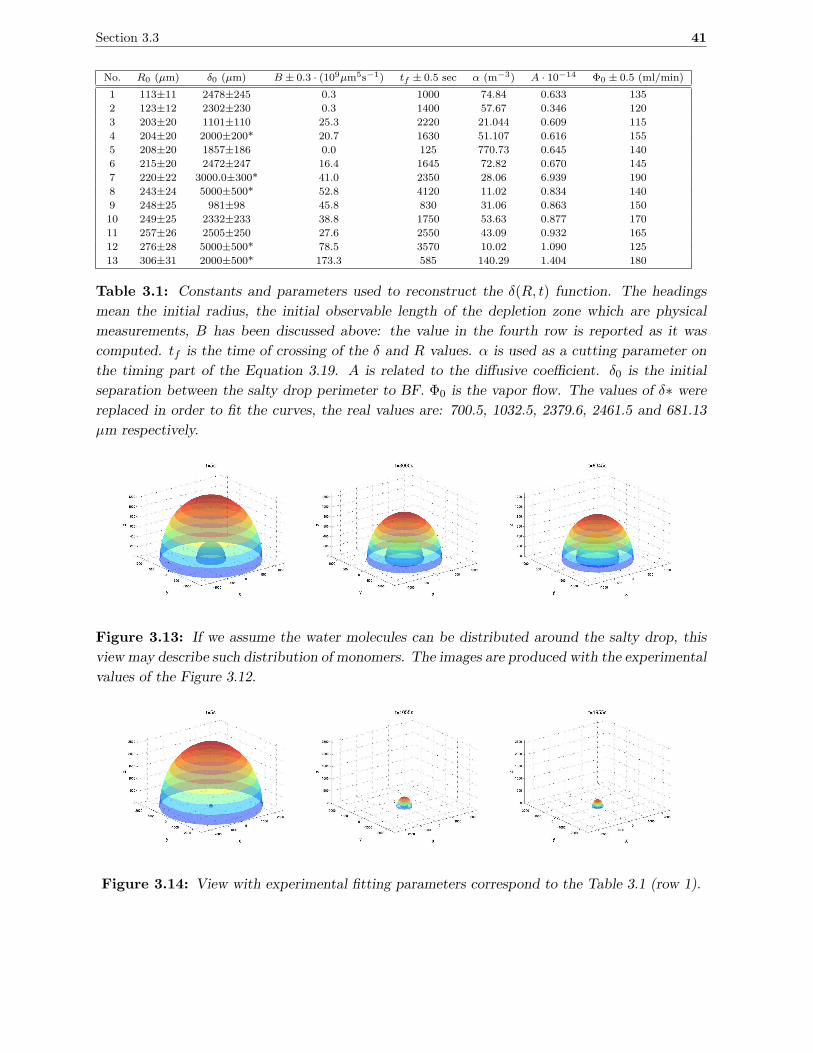
Section 3.3 41
No. R0 (µm) δ0 (µm) B ± 0.3 · (109µm5s−1) tf ± 0.5 sec α (m−3) A · 10−14 Φ0 ± 0.5 (ml/min)
1 113±11 2478±245 0.3 1000 74.84 0.633 135
2 123±12 2302±230 0.3 1400 57.67 0.346 120
3 203±20 1101±110 25.3 2220 21.044 0.609 115
4 204±20 2000±200* 20.7 1630 51.107 0.616 155
5 208±20 1857±186 0.0 125 770.73 0.645 140
6 215±20 2472±247 16.4 1645 72.82 0.670 145
7 220±22 3000.0±300* 41.0 2350 28.06 6.939 190
8 243±24 5000±500* 52.8 4120 11.02 0.834 140
9 248±25 981±98 45.8 830 31.06 0.863 150
10 249±25 2332±233 38.8 1750 53.63 0.877 170
11 257±26 2505±250 27.6 2550 43.09 0.932 165
12 276±28 5000±500* 78.5 3570 10.02 1.090 125
13 306±31 2000±500* 173.3 585 140.29 1.404 180
Table 3.1: Constants and parameters used to reconstruct the δ(R, t) function. The headings
mean the initial radius, the initial observable length of the depletion zone which are physical
measurements, B has been discussed above: the value in the fourth row is reported as it was
computed. tf is the time of crossing of the δ and R values. α is used as a cutting parameter on
the timing part of the Equation 3.19. A is related to the diffusive coefficient. δ0 is the initial
separation between the salty drop perimeter to BF. Φ0 is the vapor flow. The values of δ∗ were
replaced in order to fit the curves, the real values are: 700.5, 1032.5, 2379.6, 2461.5 and 681.13
µm respectively.
Figure 3.13: If we assume the water molecules can be distributed around the salty drop, this
view may describe such distribution of monomers. The images are produced with the experimental
values of the Figure 3.12.
Figure 3.14: View with experimental fitting parameters correspond to the Table 3.1 (row 1).
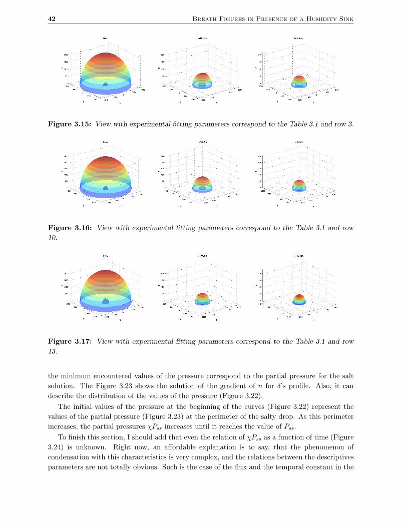
42 Breath Figures in Presence of a Humidity Sink
Figure 3.15: View with experimental fitting parameters correspond to the Table 3.1 and row 3.
Figure 3.16: View with experimental fitting parameters correspond to the Table 3.1 and row
10.
Figure 3.17: View with experimental fitting parameters correspond to the Table 3.1 and row
13.
the minimum encountered values of the pressure correspond to the partial pressure for the salt
solution. The Figure 3.23 shows the solution of the gradient of n for δ’s profile. Also, it can
describe the distribution of the values of the pressure (Figure 3.22).
The initial values of the pressure at the beginning of the curves (Figure 3.22) represent the
values of the partial pressure (Figure 3.23) at the perimeter of the salty drop. As this perimeter
increases, the partial pressures χPss increases until it reaches the value of Pss.
To finish this section, I should add that even the relation of χPss as a function of time (Figure
3.24) is unknown. Right now, an affordable explanation is to say, that the phenomenon of
condensation with this characteristics is very complex, and the relations between the descriptives
parameters are not totally obvious. Such is the case of the flux and the temporal constant in the
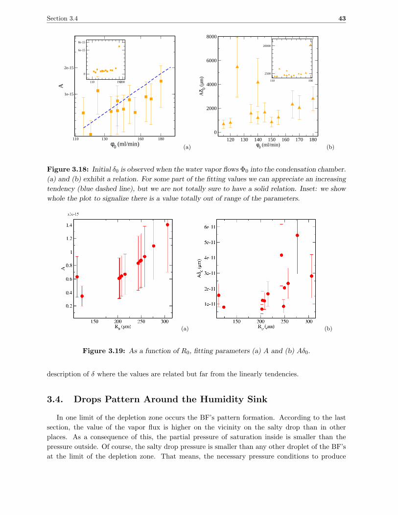
Section 3.4 43
110 130 160 180φ0 (ml/min)
1e-15
2e-15
A
110 190200
0
6e-15
8e-15
(a)
110 190
2500
20000
120 130 140 150 160 170 180φ0 (ml/min)
0
2000
4000
6000
8000
Aδ 0
(µm
)
(b)
Figure 3.18: Initial δ0 is observed when the water vapor flows Φ0 into the condensation chamber.
(a) and (b) exhibit a relation. For some part of the fitting values we can appreciate an increasing
tendency (blue dashed line), but we are not totally sure to have a solid relation. Inset: we show
whole the plot to signalize there is a value totally out of range of the parameters.
(a) (b)
Figure 3.19: As a function of R0, fitting parameters (a) A and (b) Aδ0.
description of δ where the values are related but far from the linearly tendencies.
3.4. Drops Pattern Around the Humidity Sink
In one limit of the depletion zone occurs the BF’s pattern formation. According to the last
section, the value of the vapor flux is higher on the vicinity on the salty drop than in other
places. As a consequence of this, the partial pressure of saturation inside is smaller than the
pressure outside. Of course, the salty drop pressure is smaller than any other droplet of the BF’s
at the limit of the depletion zone. That means, the necessary pressure conditions to produce
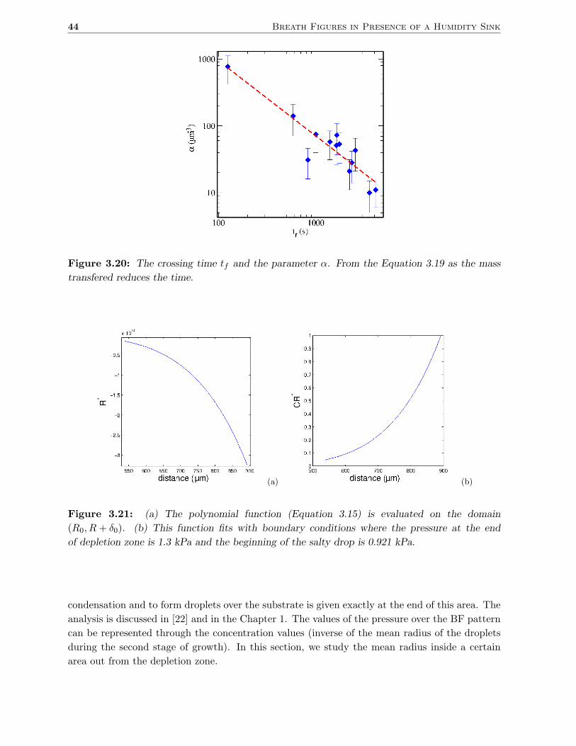
44 Breath Figures in Presence of a Humidity Sink
Figure 3.20: The crossing time tf and the parameter α. From the Equation 3.19 as the mass
transfered reduces the time.
(a) (b)
Figure 3.21: (a) The polynomial function (Equation 3.15) is evaluated on the domain
(R0, R+ δ0). (b) This function fits with boundary conditions where the pressure at the end
of depletion zone is 1.3 kPa and the beginning of the salty drop is 0.921 kPa.
condensation and to form droplets over the substrate is given exactly at the end of this area. The
analysis is discussed in [22] and in the Chapter 1. The values of the pressure over the BF pattern
can be represented through the concentration values (inverse of the mean radius of the droplets
during the second stage of growth). In this section, we study the mean radius inside a certain
area out from the depletion zone.
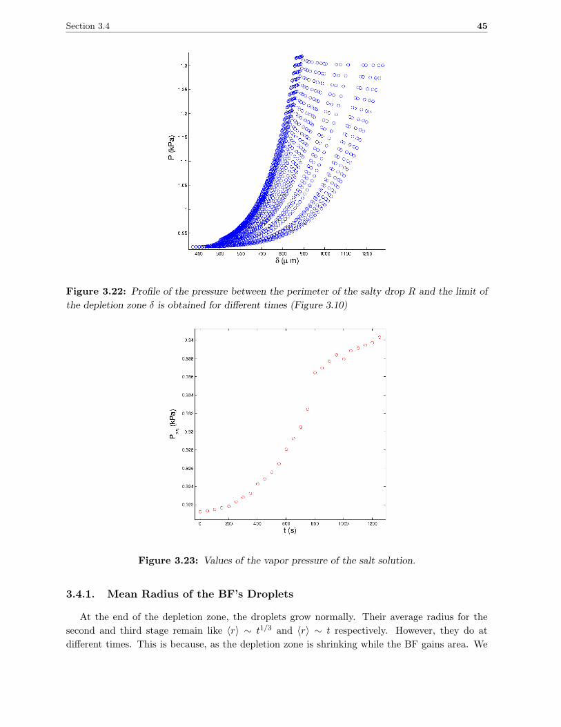
Section 3.4 45
Figure 3.22: Profile of the pressure between the perimeter of the salty drop R and the limit of
the depletion zone δ is obtained for different times (Figure 3.10)
Figure 3.23: Values of the vapor pressure of the salt solution.
3.4.1. Mean Radius of the BF’s Droplets
At the end of the depletion zone, the droplets grow normally. Their average radius for the
second and third stage remain like 〈r〉 ∼ t1/3 and 〈r〉 ∼ t respectively. However, they do at
different times. This is because, as the depletion zone is shrinking while the BF gains area. We
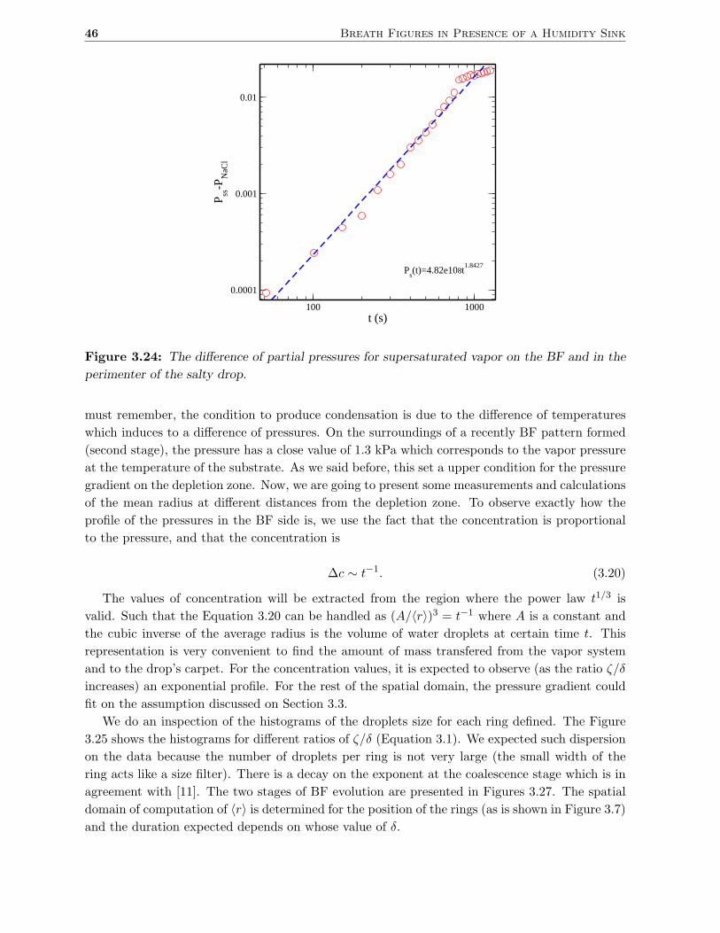
46 Breath Figures in Presence of a Humidity Sink
100 1000t (s)
0.0001
0.001
0.01
Pss
-PN
aCl
Ps(t)=4.82e108t
1.8427
Figure 3.24: The difference of partial pressures for supersaturated vapor on the BF and in the
perimenter of the salty drop.
must remember, the condition to produce condensation is due to the difference of temperatures
which induces to a difference of pressures. On the surroundings of a recently BF pattern formed
(second stage), the pressure has a close value of 1.3 kPa which corresponds to the vapor pressure
at the temperature of the substrate. As we said before, this set a upper condition for the pressure
gradient on the depletion zone. Now, we are going to present some measurements and calculations
of the mean radius at different distances from the depletion zone. To observe exactly how the
profile of the pressures in the BF side is, we use the fact that the concentration is proportional
to the pressure, and that the concentration is
∆c ∼ t−1. (3.20)
The values of concentration will be extracted from the region where the power law t1/3 is
valid. Such that the Equation 3.20 can be handled as (A/〈r〉)3 = t−1 where A is a constant and
the cubic inverse of the average radius is the volume of water droplets at certain time t. This
representation is very convenient to find the amount of mass transfered from the vapor system
and to the drop’s carpet. For the concentration values, it is expected to observe (as the ratio ζ/δ
increases) an exponential profile. For the rest of the spatial domain, the pressure gradient could
fit on the assumption discussed on Section 3.3.
We do an inspection of the histograms of the droplets size for each ring defined. The Figure
3.25 shows the histograms for different ratios of ζ/δ (Equation 3.1). We expected such dispersion
on the data because the number of droplets per ring is not very large (the small width of the
ring acts like a size filter). There is a decay on the exponent at the coalescence stage which is in
agreement with [11]. The two stages of BF evolution are presented in Figures 3.27. The spatial
domain of computation of 〈r〉 is determined for the position of the rings (as is shown in Figure 3.7)
and the duration expected depends on whose value of δ.
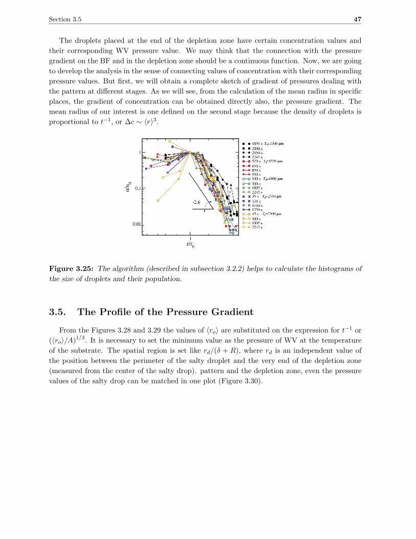
Section 3.5 47
The droplets placed at the end of the depletion zone have certain concentration values and
their corresponding WV pressure value. We may think that the connection with the pressure
gradient on the BF and in the depletion zone should be a continuous function. Now, we are going
to develop the analysis in the sense of connecting values of concentration with their corresponding
pressure values. But first, we will obtain a complete sketch of gradient of pressures dealing with
the pattern at different stages. As we will see, from the calculation of the mean radius in specific
places, the gradient of concentration can be obtained directly also, the pressure gradient. The
mean radius of our interest is one defined on the second stage because the density of droplets is
proportional to t−1, or ∆c ∼ 〈r〉3.
Figure 3.25: The algorithm (described in subsection 3.2.2) helps to calculate the histograms of
the size of droplets and their population.
3.5. The Profile of the Pressure Gradient
From the Figures 3.28 and 3.29 the values of 〈ro〉 are substituted on the expression for t−1 or
(〈ro〉/A)1/3. It is necessary to set the minimum value as the pressure of WV at the temperature
of the substrate. The spatial region is set like rd/(δ + R), where rd is an independent value of
the position between the perimeter of the salty droplet and the very end of the depletion zone
(measured from the center of the salty drop). pattern and the depletion zone, even the pressure
values of the salty drop can be matched in one plot (Figure 3.30).
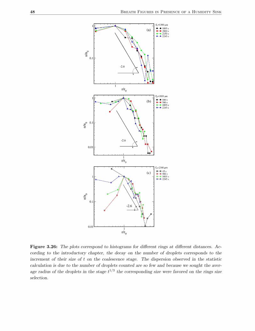
48 Breath Figures in Presence of a Humidity Sink
Figure 3.26: The plots correspond to histograms for different rings at different distances. Ac-
cording to the introductory chapter, the decay on the number of droplets corresponds to the
increment of their size of t on the coalescence stage. The dispersion observed in the statistic
calculation is due to the number of droplets counted are so few and because we sought the aver-
age radius of the droplets in the stage t1/3 the corresponding size were favored on the rings size
selection.
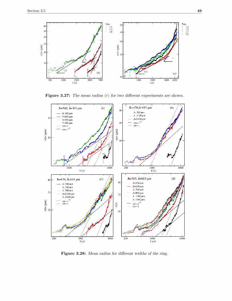
Section 3.5 49
Figure 3.27: The mean radius 〈r〉 for two different experiments are shown.
Figure 3.28: Mean radius for different widths of the ring.
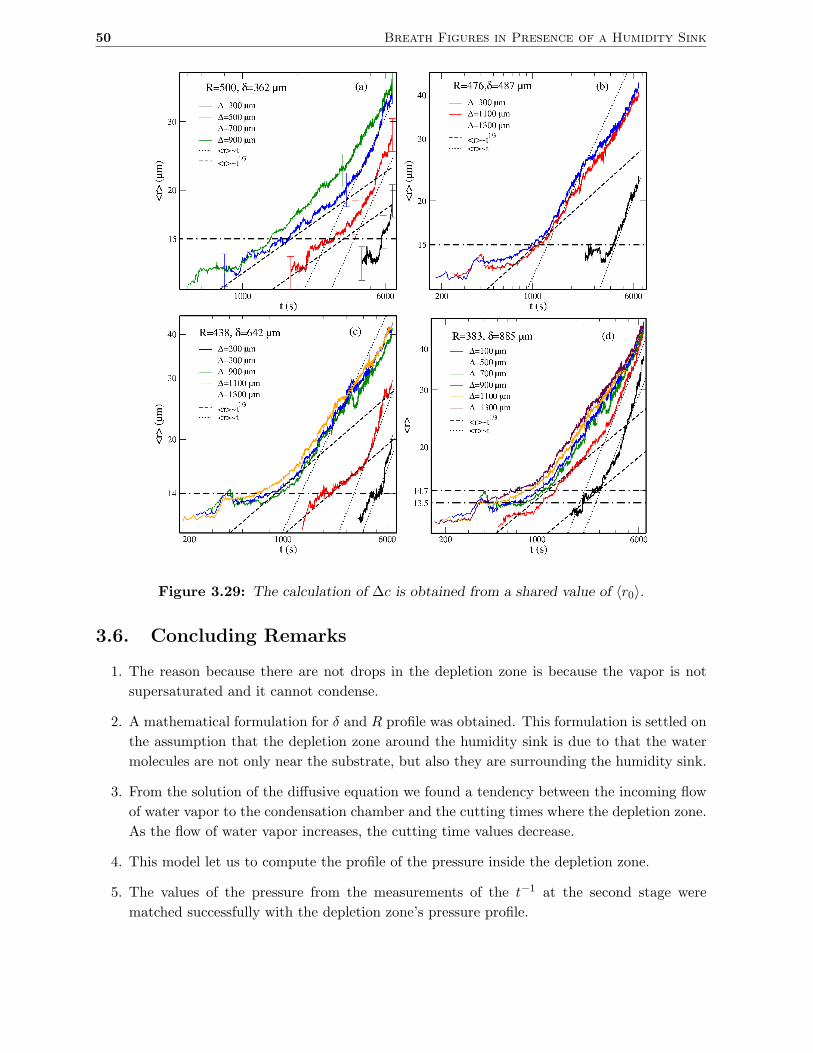
50 Breath Figures in Presence of a Humidity Sink
Figure 3.29: The calculation of ∆c is obtained from a shared value of 〈r0〉.
3.6. Concluding Remarks
1. The reason because there are not drops in the depletion zone is because the vapor is not
supersaturated and it cannot condense.
2. A mathematical formulation for δ and R profile was obtained. This formulation is settled on
the assumption that the depletion zone around the humidity sink is due to that the water
molecules are not only near the substrate, but also they are surrounding the humidity sink.
3. From the solution of the diffusive equation we found a tendency between the incoming flow
of water vapor to the condensation chamber and the cutting times where the depletion zone.
As the flow of water vapor increases, the cutting time values decrease.
4. This model let us to compute the profile of the pressure inside the depletion zone.
5. The values of the pressure from the measurements of the t−1 at the second stage were
matched successfully with the depletion zone’s pressure profile.
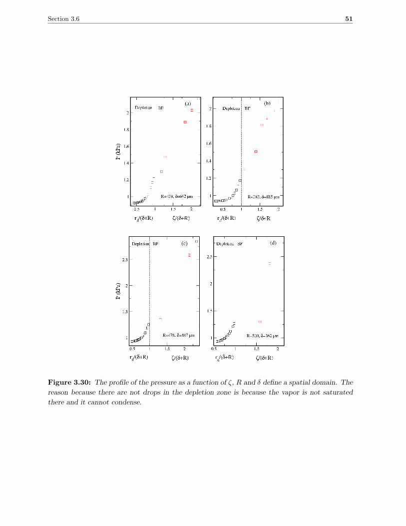
Section 3.6 51
Figure 3.30: The profile of the pressure as a function of ζ, R and δ define a spatial domain. The
reason because there are not drops in the depletion zone is because the vapor is not saturated
there and it cannot condense.

52 Breath Figures in Presence of a Humidity Sink
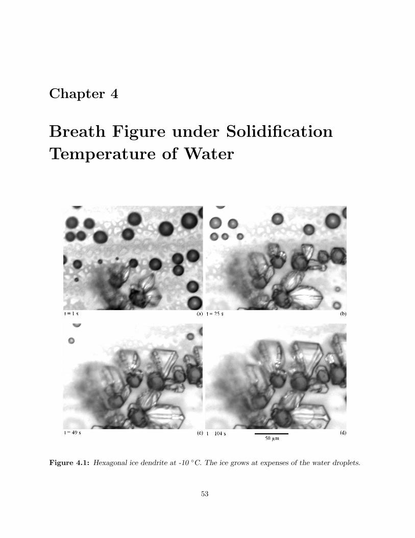
Chapter 4
Breath Figure under Solidification
Temperature of Water
Figure 4.1: Hexagonal ice dendrite at -10 C. The ice grows at expenses of the water droplets.
53
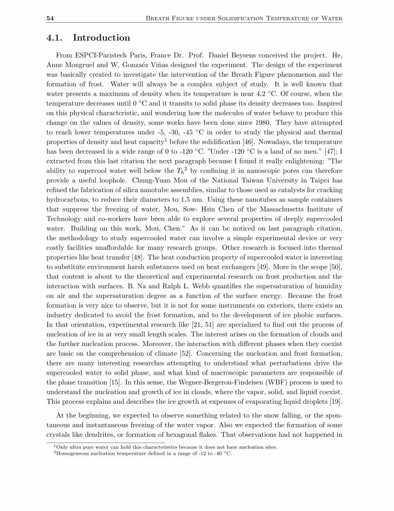
54 Breath Figure under Solidification Temperature of Water
4.1. Introduction
From ESPCI-Paristech Paris, France Dr. Prof. Daniel Beysens conceived the project. He,
Anne Mongruel and W. Gonzaez Vinas designed the experiment. The design of the experiment
was basically created to investigate the intervention of the Breath Figure phenomenon and the
formation of frost. Water will always be a complex subject of study. It is well known that
water presents a maximum of density when its temperature is near 4.2 C. Of course, when the
temperature decreases until 0 C and it transits to solid phase its density decreases too. Inspired
on this physical characteristic, and wondering how the molecules of water behave to produce this
change on the values of density, some works have been done since 1980. They have attempted
to reach lower temperatures under -5, -30, -45 C in order to study the physical and thermal
properties of density and heat capacity1 before the solidification [46]. Nowadays, the temperature
has been decreased in a wide range of 0 to -120 C. ”Under -120 C is a land of no men.” [47]; I
extracted from this last citation the next paragraph because I found it really enlightening: ”The
ability to supercool water well below the Th2 by confining it in nanoscopic pores can therefore
provide a useful loophole. Chung-Yuan Mou of the National Taiwan University in Taipei has
refined the fabrication of silica nanotube assemblies, similar to those used as catalysts for cracking
hydrocarbons, to reduce their diameters to 1.5 nm. Using these nanotubes as sample containers
that suppress the freezing of water, Mou, Sow- Hsin Chen of the Massachusetts Institute of
Technology and co-workers have been able to explore several properties of deeply supercooled
water. Building on this work, Mou, Chen.” As it can be noticed on last paragraph citation,
the methodology to study supercooled water can involve a simple experimental device or very
costly facilities unaffordable for many research groups. Other research is focused into thermal
properties like heat transfer [48]. The heat conduction property of supercooled water is interesting
to substitute environment harsh substances used on heat exchangers [49]. More in the scope [50],
that content is about to the theoretical and experimental research on frost production and the
interaction with surfaces. B. Na and Ralph L. Webb quantifies the supersaturation of humidity
on air and the supersaturation degree as a function of the surface energy. Because the frost
formation is very nice to observe, but it is not for some instruments on exteriors, there exists an
industry dedicated to avoid the frost formation, and to the development of ice phobic surfaces.
In that orientation, experimental research like [21, 51] are specialized to find out the process of
nucleation of ice in at very small length scales. The interest arises on the formation of clouds and
the further nucleation process. Moreover, the interaction with different phases when they coexist
are basic on the comprehension of climate [52]. Concerning the nucleation and frost formation,
there are many interesting researches attempting to understand what perturbations drive the
supercooled water to solid phase, and what kind of macroscopic parameters are responsible of
the phase transition [15]. In this sense, the Wegner-Bergeron-Findeisen (WBF) process is used to
understand the nucleation and growth of ice in clouds, where the vapor, solid, and liquid coexist.
This process explains and describes the ice growth at expenses of evaporating liquid droplets [19].
At the beginning, we expected to observe something related to the snow falling, or the spon-
taneous and instantaneous freezing of the water vapor. Also we expected the formation of some
crystals like dendrites, or formation of hexagonal flakes. That observations had not happened in
1Only ultra pure water can hold this characteristics because it does not have nucleation sites.2Homogeneous nucleation temperature defined in a range of -12 to -40 C.
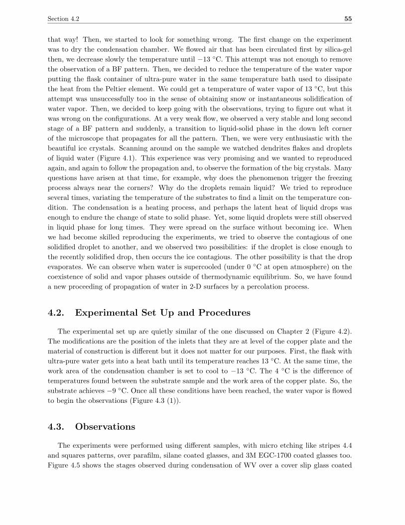
Section 4.2 55
that way! Then, we started to look for something wrong. The first change on the experiment
was to dry the condensation chamber. We flowed air that has been circulated first by silica-gel
then, we decrease slowly the temperature until −13 C. This attempt was not enough to remove
the observation of a BF pattern. Then, we decided to reduce the temperature of the water vapor
putting the flask container of ultra-pure water in the same temperature bath used to dissipate
the heat from the Peltier element. We could get a temperature of water vapor of 13 C, but this
attempt was unsuccessfully too in the sense of obtaining snow or instantaneous solidification of
water vapor. Then, we decided to keep going with the observations, trying to figure out what it
was wrong on the configurations. At a very weak flow, we observed a very stable and long second
stage of a BF pattern and suddenly, a transition to liquid-solid phase in the down left corner
of the microscope that propagates for all the pattern. Then, we were very enthusiastic with the
beautiful ice crystals. Scanning around on the sample we watched dendrites flakes and droplets
of liquid water (Figure 4.1). This experience was very promising and we wanted to reproduced
again, and again to follow the propagation and, to observe the formation of the big crystals. Many
questions have arisen at that time, for example, why does the phenomenon trigger the freezing
process always near the corners? Why do the droplets remain liquid? We tried to reproduce
several times, variating the temperature of the substrates to find a limit on the temperature con-
dition. The condensation is a heating process, and perhaps the latent heat of liquid drops was
enough to endure the change of state to solid phase. Yet, some liquid droplets were still observed
in liquid phase for long times. They were spread on the surface without becoming ice. When
we had become skilled reproducing the experiments, we tried to observe the contagious of one
solidified droplet to another, and we observed two possibilities: if the droplet is close enough to
the recently solidified drop, then occurs the ice contagious. The other possibility is that the drop
evaporates. We can observe when water is supercooled (under 0 C at open atmosphere) on the
coexistence of solid and vapor phases outside of thermodynamic equilibrium. So, we have found
a new proceeding of propagation of water in 2-D surfaces by a percolation process.
4.2. Experimental Set Up and Procedures
The experimental set up are quietly similar of the one discussed on Chapter 2 (Figure 4.2).
The modifications are the position of the inlets that they are at level of the copper plate and the
material of construction is different but it does not matter for our purposes. First, the flask with
ultra-pure water gets into a heat bath until its temperature reaches 13 C. At the same time, the
work area of the condensation chamber is set to cool to −13 C. The 4 C is the difference of
temperatures found between the substrate sample and the work area of the copper plate. So, the
substrate achieves −9 C. Once all these conditions have been reached, the water vapor is flowed
to begin the observations (Figure 4.3 (1)).
4.3. Observations
The experiments were performed using different samples, with micro etching like stripes 4.4
and squares patterns, over parafilm, silane coated glasses, and 3M EGC-1700 coated glasses too.
Figure 4.5 shows the stages observed during condensation of WV over a cover slip glass coated
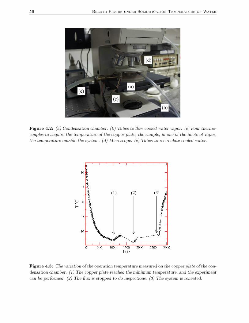
56 Breath Figure under Solidification Temperature of Water
Figure 4.2: (a) Condensation chamber. (b) Tubes to flow cooled water vapor. (c) Four thermo-
couples to acquire the temperature of the copper plate, the sample, in one of the inlets of vapor,
the temperature outside the system. (d) Microscope. (e) Tubes to recirculate cooled water.
Figure 4.3: The variation of the operation temperature measured on the copper plate of the con-
densation chamber. (1) The copper plate reached the minimum temperature, and the experiment
can be performed. (2) The flux is stopped to do inspections. (3) The system is reheated.
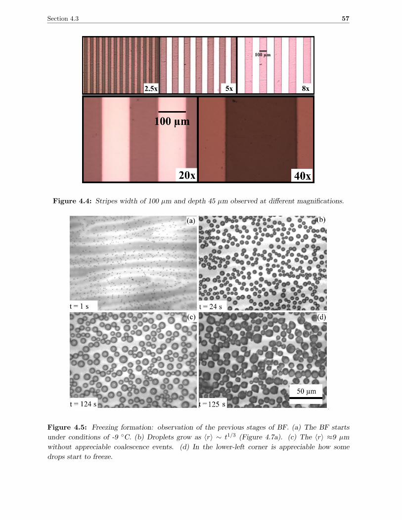
Section 4.3 57
Figure 4.4: Stripes width of 100 µm and depth 45 µm observed at different magnifications.
Figure 4.5: Freezing formation: observation of the previous stages of BF. (a) The BF starts
under conditions of -9 C. (b) Droplets grow as 〈r〉 ∼ t1/3 (Figure 4.7a). (c) The 〈r〉 ≈9 µm
without appreciable coalescence events. (d) In the lower-left corner is appreciable how some
drops start to freeze.
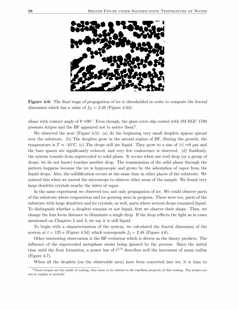
58 Breath Figure under Solidification Temperature of Water
Figure 4.6: The final stage of propagation of ice is thresholded in order to compute the fractal
dimension which has a value of fD = 2.48 (Figure 4.5d).
silane with contact angle of θ ≈90. Even though, the glass cover slip coated with 3M EGC 1700
presents stripes and the BF appeared not to notice them3.
We observed the next (Figure 4.5): (a) At the beginning very small droplets appear spread
over the substrate. (b) The droplets grow in the second regime of BF. During the growth, the
temperature is T ≈ -10C. (c) The drops still are liquid. They grow to a size of 〈r〉 ≈9 µm and
the bare spaces are significantly reduced, and very few coalescence is observed. (d) Suddenly,
the system transits from supercooled to solid phase. It occurs when one iced drop (or a group of
drops, we do not know) touches another drop. The transmission of the solid phase through the
pattern happens because the ice is hygroscopic and grows by the adsorption of vapor from the
liquid drops. Also, the solidification occurs at the same time in other places of the substrate. We
noticed this when we moved the microscope to observe other areas of the sample. We found very
large dendrite crystals nearby the inlets of vapor.
In the same experiment we observed too, not only propagation of ice. We could observe parts
of the substrate where evaporation and ice growing were in progress. There were too, parts of the
substrate with large dendrites and ice crystals, as well, parts where several drops remained liquid.
To distinguish whether a droplets remains or not liquid, first we observe their shape. Then, we
change the lens focus distance to illuminate a single drop. If the drop reflects the light as in cases
mentioned on Chapters 2 and 3, we say it is still liquid.
To begin with a characterization of the system, we calculated the fractal dimension of the
system at t = 125 s (Figure 4.5d) which corresponds fd = 2.48 (Figure 4.6).
Other interesting observation is the BF evolution which is driven as the theory predicts. The
influence of the supercooled metaphase seems being ignored by the process. Since the initial
time until the frost formation, a power law of t1/3 describes well the increment of mean radius
(Figure 4.7).
When all the droplets (on the observable area) have been converted into ice, it is time to
3Those stripes are the result of coating, they seem to be related to the repellent property of this coating. The stripes are
not so regular or periodic
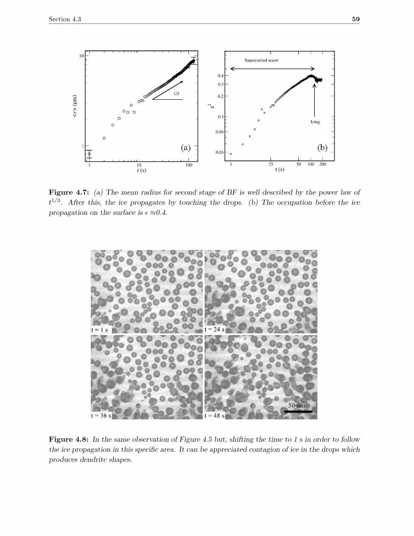
Section 4.3 59
Figure 4.7: (a) The mean radius for second stage of BF is well described by the power law of
t1/3. After this, the ice propagates by touching the drops. (b) The occupation before the ice
propagation on the surface is ǫ ≈0.4.
Figure 4.8: In the same observation of Figure 4.5 but, shifting the time to 1 s in order to follow
the ice propagation in this specific area. It can be appreciated contagion of ice in the drops which
produces dendritc shapes.
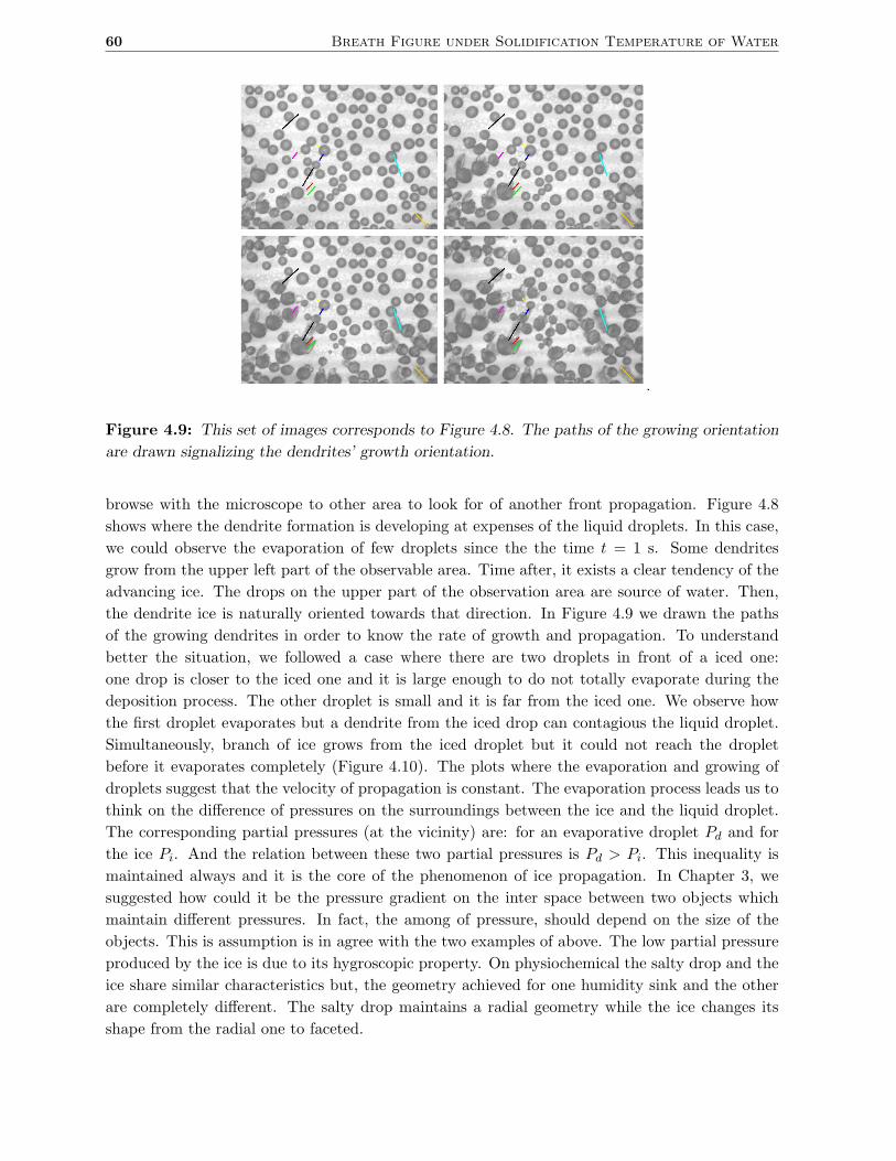
60 Breath Figure under Solidification Temperature of Water
Figure 4.9: This set of images corresponds to Figure 4.8. The paths of the growing orientation
are drawn signalizing the dendrites’ growth orientation.
browse with the microscope to other area to look for of another front propagation. Figure 4.8
shows where the dendrite formation is developing at expenses of the liquid droplets. In this case,
we could observe the evaporation of few droplets since the the time t = 1 s. Some dendrites
grow from the upper left part of the observable area. Time after, it exists a clear tendency of the
advancing ice. The drops on the upper part of the observation area are source of water. Then,
the dendrite ice is naturally oriented towards that direction. In Figure 4.9 we drawn the paths
of the growing dendrites in order to know the rate of growth and propagation. To understand
better the situation, we followed a case where there are two droplets in front of a iced one:
one drop is closer to the iced one and it is large enough to do not totally evaporate during the
deposition process. The other droplet is small and it is far from the iced one. We observe how
the first droplet evaporates but a dendrite from the iced drop can contagious the liquid droplet.
Simultaneously, branch of ice grows from the iced droplet but it could not reach the droplet
before it evaporates completely (Figure 4.10). The plots where the evaporation and growing of
droplets suggest that the velocity of propagation is constant. The evaporation process leads us to
think on the difference of pressures on the surroundings between the ice and the liquid droplet.
The corresponding partial pressures (at the vicinity) are: for an evaporative droplet Pd and for
the ice Pi. And the relation between these two partial pressures is Pd > Pi. This inequality is
maintained always and it is the core of the phenomenon of ice propagation. In Chapter 3, we
suggested how could it be the pressure gradient on the inter space between two objects which
maintain different pressures. In fact, the among of pressure, should depend on the size of the
objects. This is assumption is in agree with the two examples of above. The low partial pressure
produced by the ice is due to its hygroscopic property. On physiochemical the salty drop and the
ice share similar characteristics but, the geometry achieved for one humidity sink and the other
are completely different. The salty drop maintains a radial geometry while the ice changes its
shape from the radial one to faceted.
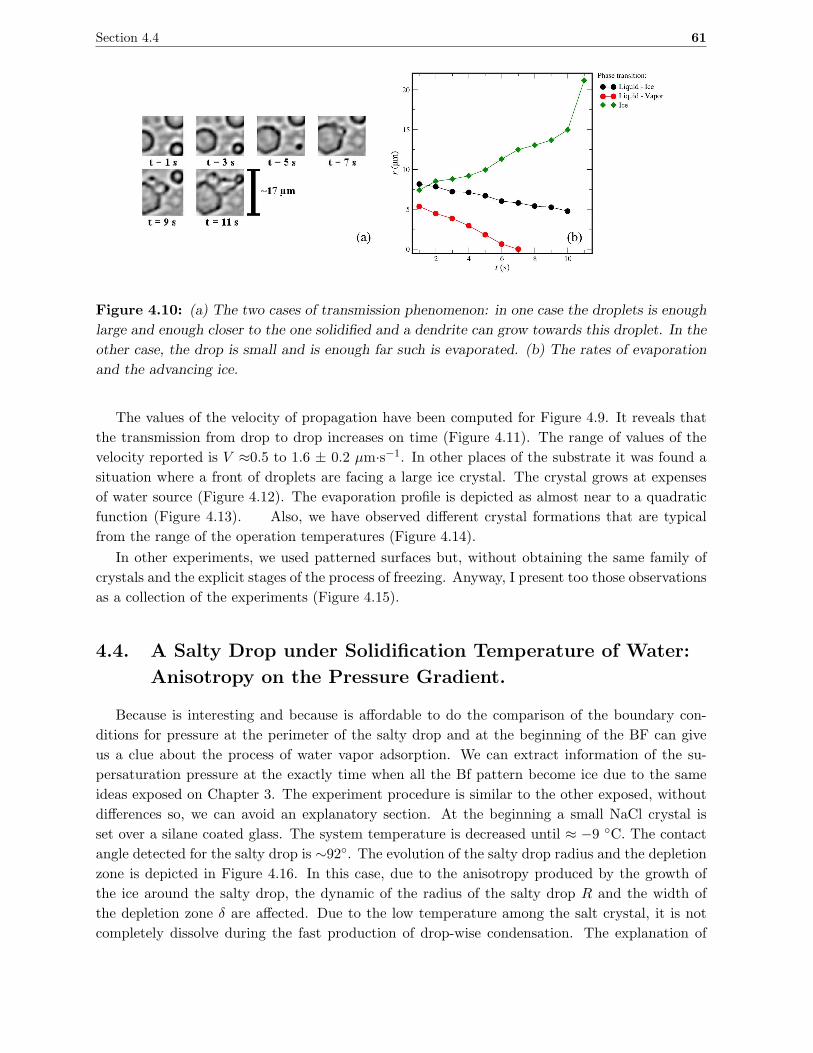
Section 4.4 61
Figure 4.10: (a) The two cases of transmission phenomenon: in one case the droplets is enough
large and enough closer to the one solidified and a dendrite can grow towards this droplet. In the
other case, the drop is small and is enough far such is evaporated. (b) The rates of evaporation
and the advancing ice.
The values of the velocity of propagation have been computed for Figure 4.9. It reveals that
the transmission from drop to drop increases on time (Figure 4.11). The range of values of the
velocity reported is V ≈0.5 to 1.6 ± 0.2 µm·s−1. In other places of the substrate it was found a
situation where a front of droplets are facing a large ice crystal. The crystal grows at expenses
of water source (Figure 4.12). The evaporation profile is depicted as almost near to a quadratic
function (Figure 4.13). Also, we have observed different crystal formations that are typical
from the range of the operation temperatures (Figure 4.14).
In other experiments, we used patterned surfaces but, without obtaining the same family of
crystals and the explicit stages of the process of freezing. Anyway, I present too those observations
as a collection of the experiments (Figure 4.15).
4.4. A Salty Drop under Solidification Temperature of Water:
Anisotropy on the Pressure Gradient.
Because is interesting and because is affordable to do the comparison of the boundary con-
ditions for pressure at the perimeter of the salty drop and at the beginning of the BF can give
us a clue about the process of water vapor adsorption. We can extract information of the su-
persaturation pressure at the exactly time when all the Bf pattern become ice due to the same
ideas exposed on Chapter 3. The experiment procedure is similar to the other exposed, without
differences so, we can avoid an explanatory section. At the beginning a small NaCl crystal is
set over a silane coated glass. The system temperature is decreased until ≈ −9 C. The contact
angle detected for the salty drop is ∼92. The evolution of the salty drop radius and the depletion
zone is depicted in Figure 4.16. In this case, due to the anisotropy produced by the growth of
the ice around the salty drop, the dynamic of the radius of the salty drop R and the width of
the depletion zone δ are affected. Due to the low temperature among the salt crystal, it is not
completely dissolve during the fast production of drop-wise condensation. The explanation of
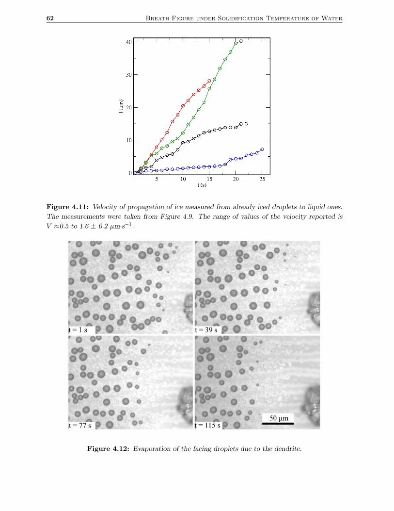
62 Breath Figure under Solidification Temperature of Water
Figure 4.11: Velocity of propagation of ice measured from already iced droplets to liquid ones.
The measurements were taken from Figure 4.9. The range of values of the velocity reported is
V ≈0.5 to 1.6 ± 0.2 µm·s−1.
Figure 4.12: Evaporation of the facing droplets due to the dendrite.
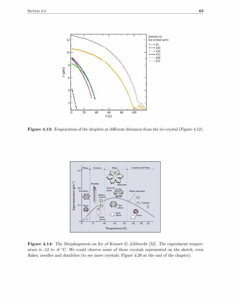
Section 4.4 63
Figure 4.13: Evaporation of the droplets at different distances from the ice crystal (Figure 4.12).
Figure 4.14: The Morphogenesis on Ice of Kennet G. Libbrecht [53]. The experiment temper-
ature is -12 to -6 C. We could observe some of those crystals represented on the sketch, even
flakes, needles and dendrites (to see more crystals, Figure 4.26 at the end of the chapter).
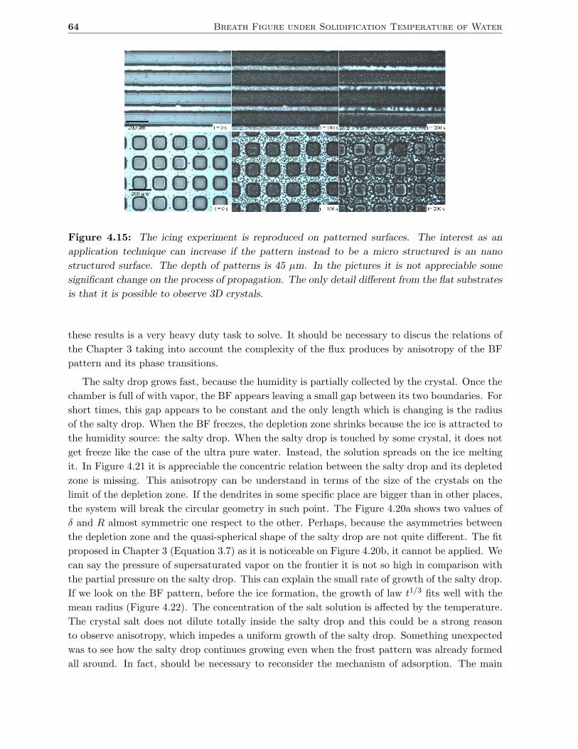
64 Breath Figure under Solidification Temperature of Water
Figure 4.15: The icing experiment is reproduced on patterned surfaces. The interest as an
application technique can increase if the pattern instead to be a micro structured is an nano
structured surface. The depth of patterns is 45 µm. In the pictures it is not appreciable some
significant change on the process of propagation. The only detail different from the flat substrates
is that it is possible to observe 3D crystals.
these results is a very heavy duty task to solve. It should be necessary to discus the relations of
the Chapter 3 taking into account the complexity of the flux produces by anisotropy of the BF
pattern and its phase transitions.
The salty drop grows fast, because the humidity is partially collected by the crystal. Once the
chamber is full of with vapor, the BF appears leaving a small gap between its two boundaries. For
short times, this gap appears to be constant and the only length which is changing is the radius
of the salty drop. When the BF freezes, the depletion zone shrinks because the ice is attracted to
the humidity source: the salty drop. When the salty drop is touched by some crystal, it does not
get freeze like the case of the ultra pure water. Instead, the solution spreads on the ice melting
it. In Figure 4.21 it is appreciable the concentric relation between the salty drop and its depleted
zone is missing. This anisotropy can be understand in terms of the size of the crystals on the
limit of the depletion zone. If the dendrites in some specific place are bigger than in other places,
the system will break the circular geometry in such point. The Figure 4.20a shows two values of
δ and R almost symmetric one respect to the other. Perhaps, because the asymmetries between
the depletion zone and the quasi-spherical shape of the salty drop are not quite different. The fit
proposed in Chapter 3 (Equation 3.7) as it is noticeable on Figure 4.20b, it cannot be applied. We
can say the pressure of supersaturated vapor on the frontier it is not so high in comparison with
the partial pressure on the salty drop. This can explain the small rate of growth of the salty drop.
If we look on the BF pattern, before the ice formation, the growth of law t1/3 fits well with the
mean radius (Figure 4.22). The concentration of the salt solution is affected by the temperature.
The crystal salt does not dilute totally inside the salty drop and this could be a strong reason
to observe anisotropy, which impedes a uniform growth of the salty drop. Something unexpected
was to see how the salty drop continues growing even when the frost pattern was already formed
all around. In fact, should be necessary to reconsider the mechanism of adsorption. The main
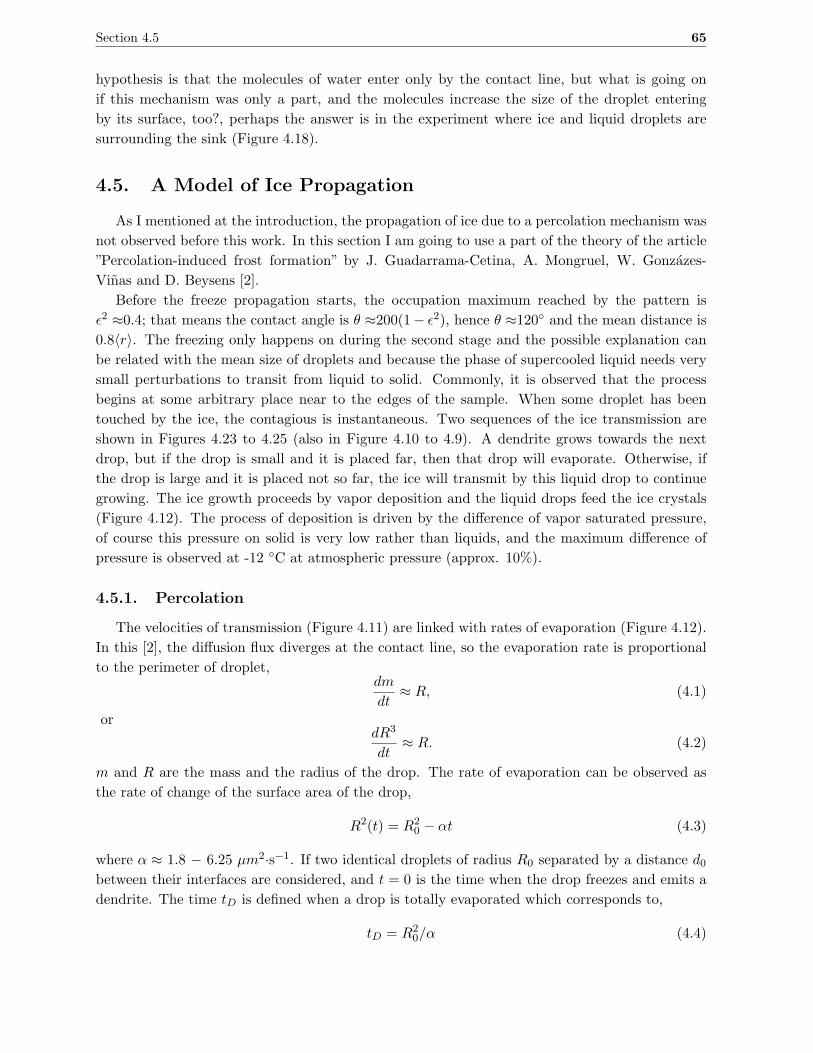
Section 4.5 65
hypothesis is that the molecules of water enter only by the contact line, but what is going on
if this mechanism was only a part, and the molecules increase the size of the droplet entering
by its surface, too?, perhaps the answer is in the experiment where ice and liquid droplets are
surrounding the sink (Figure 4.18).
4.5. A Model of Ice Propagation
As I mentioned at the introduction, the propagation of ice due to a percolation mechanism was
not observed before this work. In this section I am going to use a part of the theory of the article
”Percolation-induced frost formation” by J. Guadarrama-Cetina, A. Mongruel, W. Gonzazes-
Vinas and D. Beysens [2].
Before the freeze propagation starts, the occupation maximum reached by the pattern is
ǫ2 ≈0.4; that means the contact angle is θ ≈200(1− ǫ2), hence θ ≈120 and the mean distance is
0.8〈r〉. The freezing only happens on during the second stage and the possible explanation can
be related with the mean size of droplets and because the phase of supercooled liquid needs very
small perturbations to transit from liquid to solid. Commonly, it is observed that the process
begins at some arbitrary place near to the edges of the sample. When some droplet has been
touched by the ice, the contagious is instantaneous. Two sequences of the ice transmission are
shown in Figures 4.23 to 4.25 (also in Figure 4.10 to 4.9). A dendrite grows towards the next
drop, but if the drop is small and it is placed far, then that drop will evaporate. Otherwise, if
the drop is large and it is placed not so far, the ice will transmit by this liquid drop to continue
growing. The ice growth proceeds by vapor deposition and the liquid drops feed the ice crystals
(Figure 4.12). The process of deposition is driven by the difference of vapor saturated pressure,
of course this pressure on solid is very low rather than liquids, and the maximum difference of
pressure is observed at -12 C at atmospheric pressure (approx. 10%).
4.5.1. Percolation
The velocities of transmission (Figure 4.11) are linked with rates of evaporation (Figure 4.12).
In this [2], the diffusion flux diverges at the contact line, so the evaporation rate is proportional
to the perimeter of droplet,dm
dt≈ R, (4.1)
ordR3
dt≈ R. (4.2)
m and R are the mass and the radius of the drop. The rate of evaporation can be observed as
the rate of change of the surface area of the drop,
R2(t) = R20 − αt (4.3)
where α ≈ 1.8 − 6.25 µm2·s−1. If two identical droplets of radius R0 separated by a distance d0between their interfaces are considered, and t = 0 is the time when the drop freezes and emits a
dendrite. The time tD is defined when a drop is totally evaporated which corresponds to,
tD = R20/α (4.4)
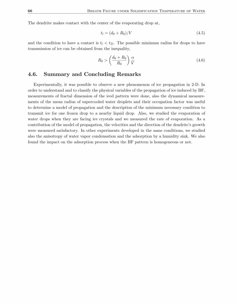
66 Breath Figure under Solidification Temperature of Water
The dendrite makes contact with the center of the evaporating drop at,
tl = (d0 +R0)/V (4.5)
and the condition to have a contact is tl < tD. The possible minimum radius for drops to have
transmission of ice can be obtained from the inequality,
R0 >
(
d0 +R0
R0
)
α
V(4.6)
4.6. Summary and Concluding Remarks
Experimentally, it was possible to observe a new phenomenon of ice propagation in 2-D. In
order to understand and to classify the physical variables of the propagation of ice induced by BF,
measurements of fractal dimension of the iced pattern were done, also the dynamical measure-
ments of the mean radius of supercooled water droplets and their occupation factor was useful
to determine a model of propagation and the description of the minimum necessary condition to
transmit ice for one frozen drop to a nearby liquid drop. Also, we studied the evaporation of
water drops when they are facing ice crystals and we measured the rate of evaporation. As a
contribution of the model of propagation, the velocities and the direction of the dendrite’s growth
were measured satisfactory. In other experiments developed in the same conditions, we studied
also the anisotropy of water vapor condensation and the adsorption by a humidity sink. We also
found the impact on the adsorption process when the BF pattern is homogeneous or not.
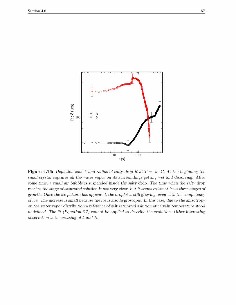
Section 4.6 67
1 10 100t (s)
100
R ;
δ (µ
m)
Rδ
Figure 4.16: Depletion zone δ and radius of salty drop R at T = -9 C. At the beginning the
small crystal captures all the water vapor on its surroundings getting wet and dissolving. After
some time, a small air bubble is suspended inside the salty drop. The time when the salty drop
reaches the stage of saturated solution is not very clear, but it seems exists at least three stages of
growth. Once the ice pattern has appeared, the droplet is still growing, even with the competency
of ice. The increase is small because the ice is also hygroscopic. In this case, due to the anisotropy
on the water vapor distribution a reference of salt saturated solution at certain temperature stood
undefined. The fit (Equation 3.7) cannot be applied to describe the evolution. Other interesting
observation is the crossing of δ and R.
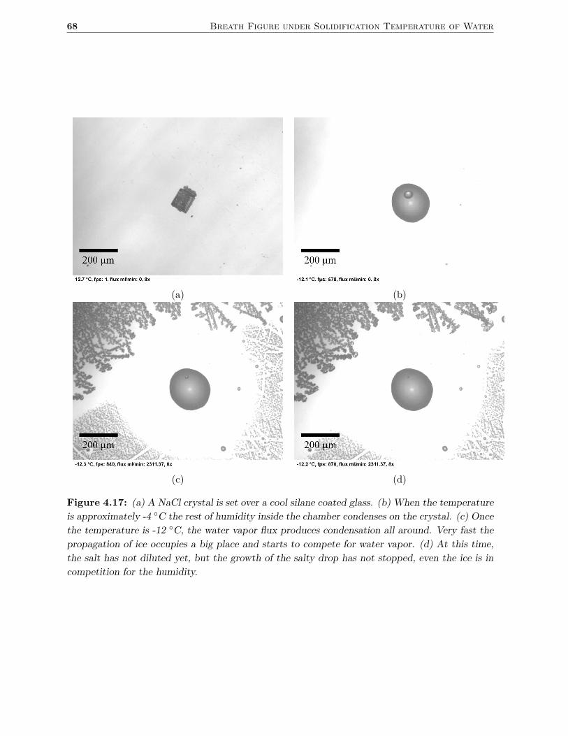
68 Breath Figure under Solidification Temperature of Water
(a) (b)
(c) (d)
Figure 4.17: (a) A NaCl crystal is set over a cool silane coated glass. (b) When the temperature
is approximately -4 C the rest of humidity inside the chamber condenses on the crystal. (c) Once
the temperature is -12 C, the water vapor flux produces condensation all around. Very fast the
propagation of ice occupies a big place and starts to compete for water vapor. (d) At this time,
the salt has not diluted yet, but the growth of the salty drop has not stopped, even the ice is in
competition for the humidity.
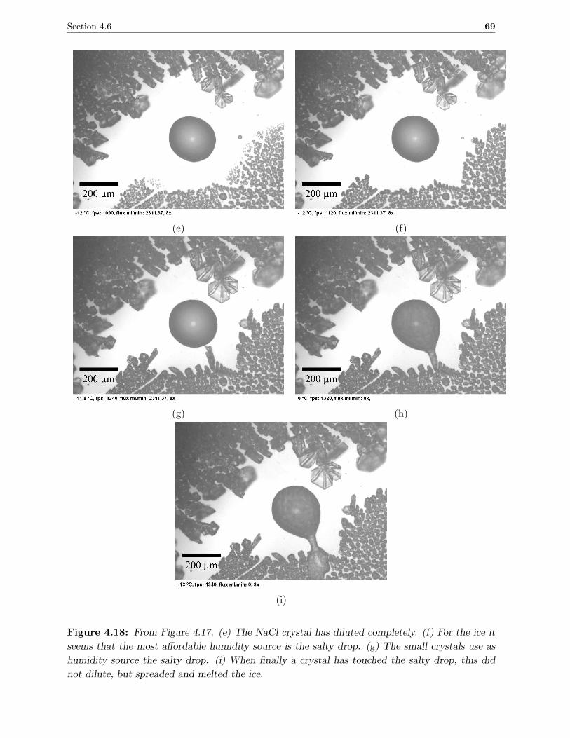
Section 4.6 69
(e) (f)
(g) (h)
(i)
Figure 4.18: From Figure 4.17. (e) The NaCl crystal has diluted completely. (f) For the ice it
seems that the most affordable humidity source is the salty drop. (g) The small crystals use as
humidity source the salty drop. (i) When finally a crystal has touched the salty drop, this did
not dilute, but spreaded and melted the ice.
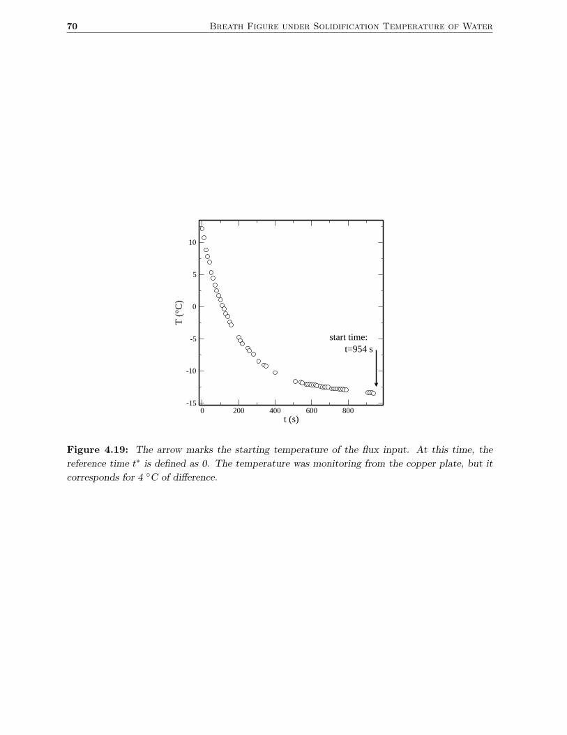
70 Breath Figure under Solidification Temperature of Water
0 200 400 600 800t (s)
-15
-10
-5
0
5
10
T (
°C)
t=954 sstart time:
Figure 4.19: The arrow marks the starting temperature of the flux input. At this time, the
reference time t∗ is defined as 0. The temperature was monitoring from the copper plate, but it
corresponds for 4 C of difference.
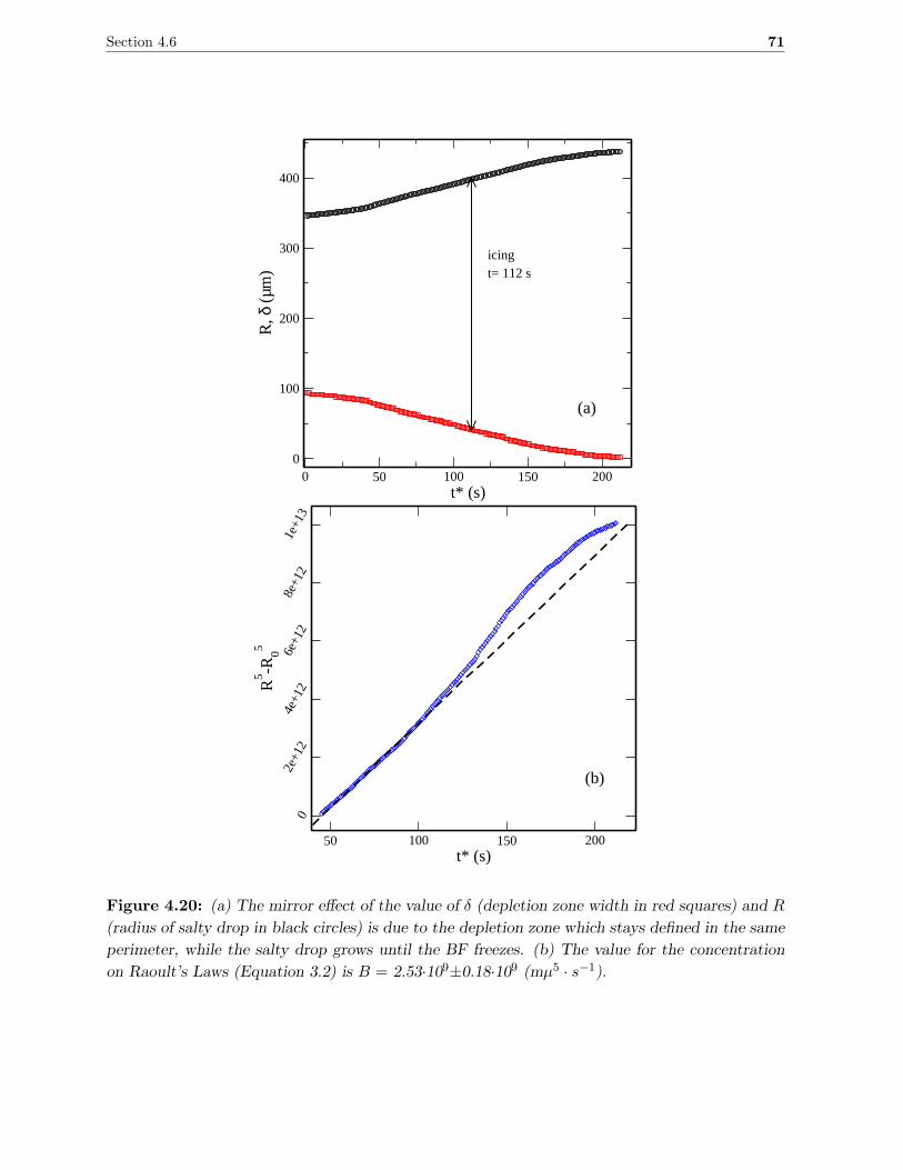
Section 4.6 71
0 50 100 150 200t* (s)
0
100
200
300
400
R, δ
(µm
)icingt= 112 s
(a)
50 100 150 200t* (s)
02e
+12
4e+1
26e
+12
8e+1
21e
+13
R5 -R
05
(b)
Figure 4.20: (a) The mirror effect of the value of δ (depletion zone width in red squares) and R
(radius of salty drop in black circles) is due to the depletion zone which stays defined in the same
perimeter, while the salty drop grows until the BF freezes. (b) The value for the concentration
on Raoult’s Laws (Equation 3.2) is B = 2.53·109±0.18·109 (mµ5 · s−1).
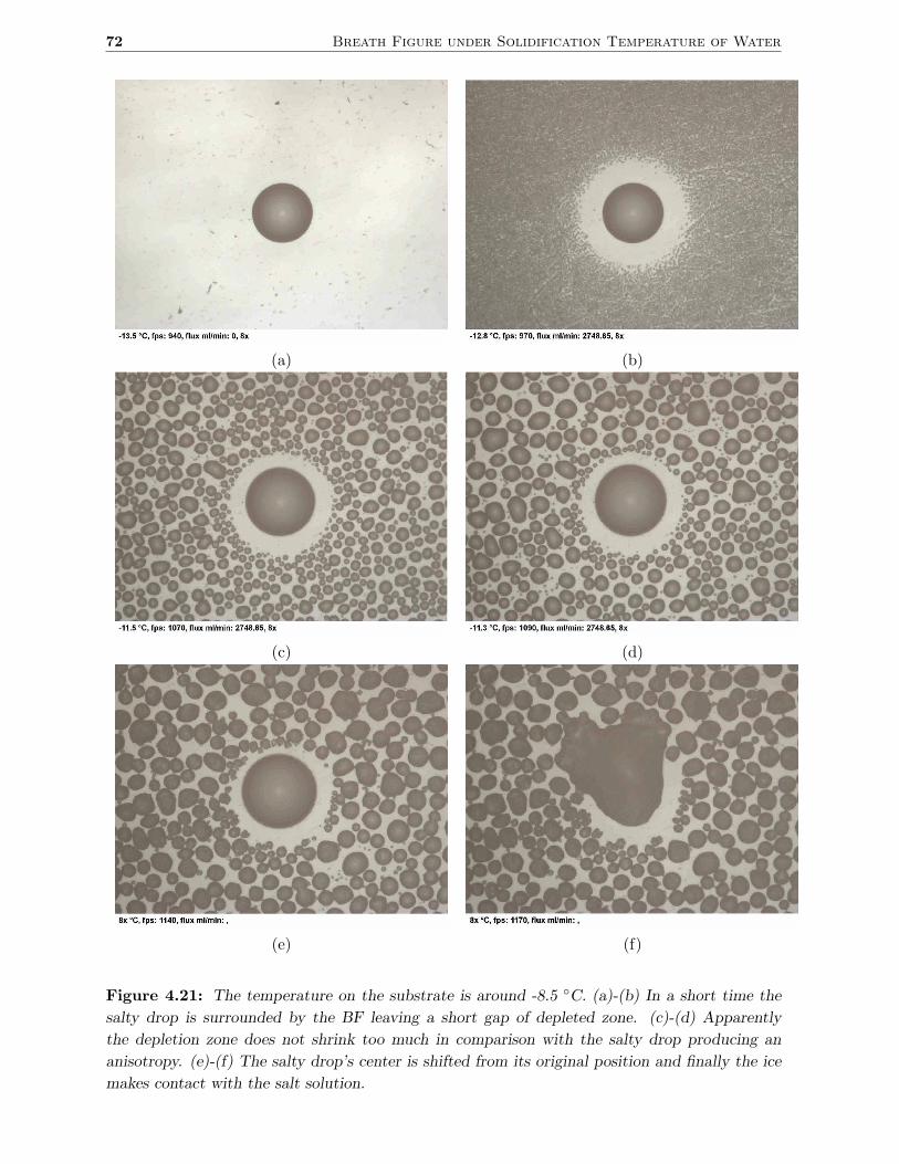
72 Breath Figure under Solidification Temperature of Water
(a) (b)
(c) (d)
(e) (f)
Figure 4.21: The temperature on the substrate is around -8.5 C. (a)-(b) In a short time the
salty drop is surrounded by the BF leaving a short gap of depleted zone. (c)-(d) Apparently
the depletion zone does not shrink too much in comparison with the salty drop producing an
anisotropy. (e)-(f) The salty drop’s center is shifted from its original position and finally the ice
makes contact with the salt solution.
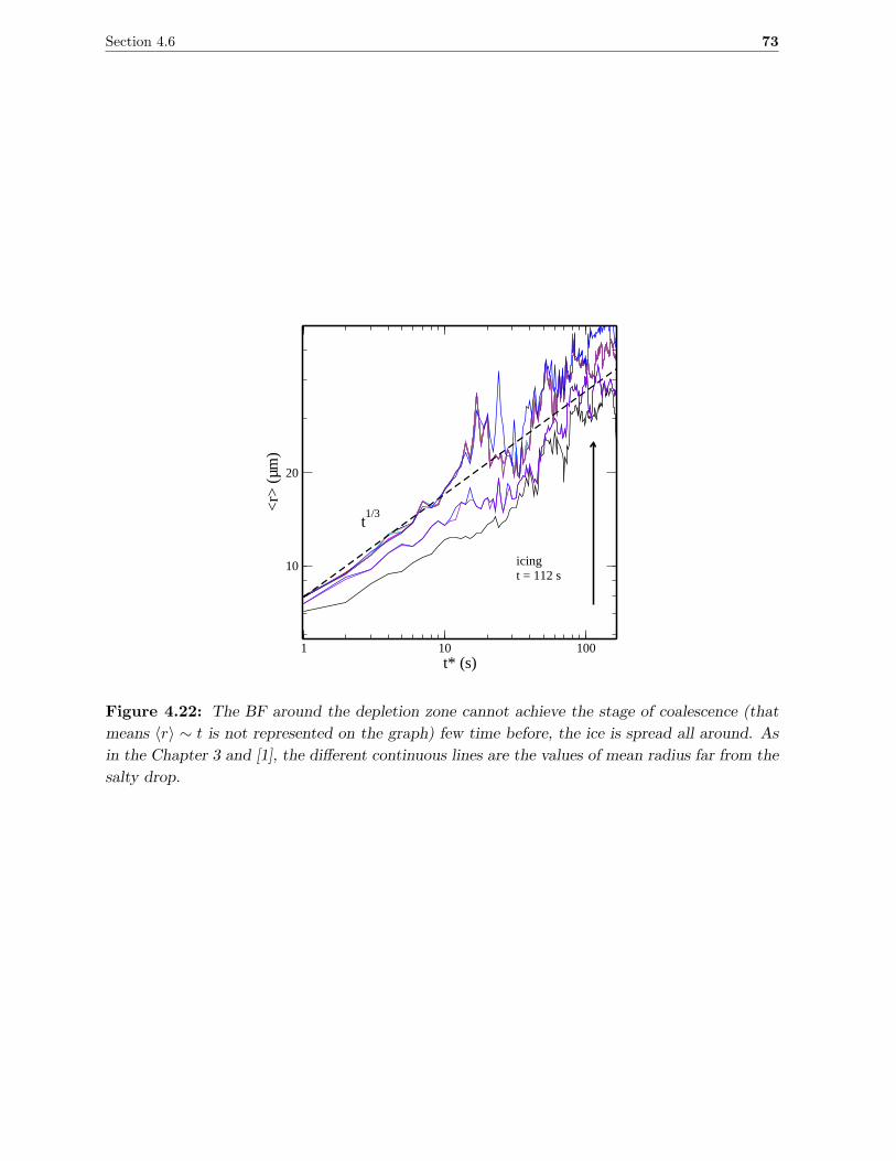
Section 4.6 73
1 10 100t* (s)
10
20
<r>
(µ
m)
icingt = 112 s
t1/3
Figure 4.22: The BF around the depletion zone cannot achieve the stage of coalescence (that
means 〈r〉 ∼ t is not represented on the graph) few time before, the ice is spread all around. As
in the Chapter 3 and [1], the different continuous lines are the values of mean radius far from the
salty drop.
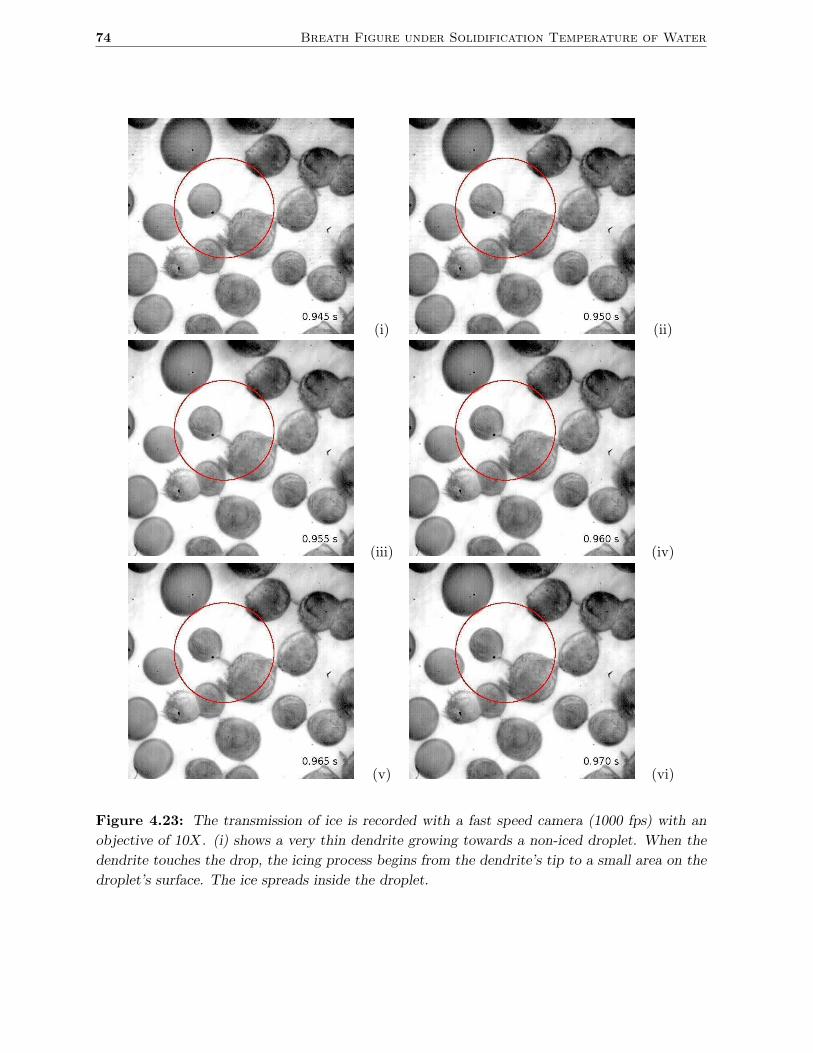
74 Breath Figure under Solidification Temperature of Water
(i) (ii)
(iii) (iv)
(v) (vi)
Figure 4.23: The transmission of ice is recorded with a fast speed camera (1000 fps) with an
objective of 10X. (i) shows a very thin dendrite growing towards a non-iced droplet. When the
dendrite touches the drop, the icing process begins from the dendrite’s tip to a small area on the
droplet’s surface. The ice spreads inside the droplet.
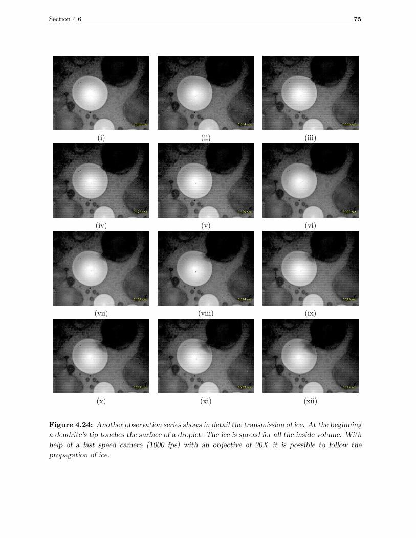
Section 4.6 75
(i) (ii) (iii)
(iv) (v) (vi)
(vii) (viii) (ix)
(x) (xi) (xii)
Figure 4.24: Another observation series shows in detail the transmission of ice. At the beginning
a dendrite’s tip touches the surface of a droplet. The ice is spread for all the inside volume. With
help of a fast speed camera (1000 fps) with an objective of 20X it is possible to follow the
propagation of ice.
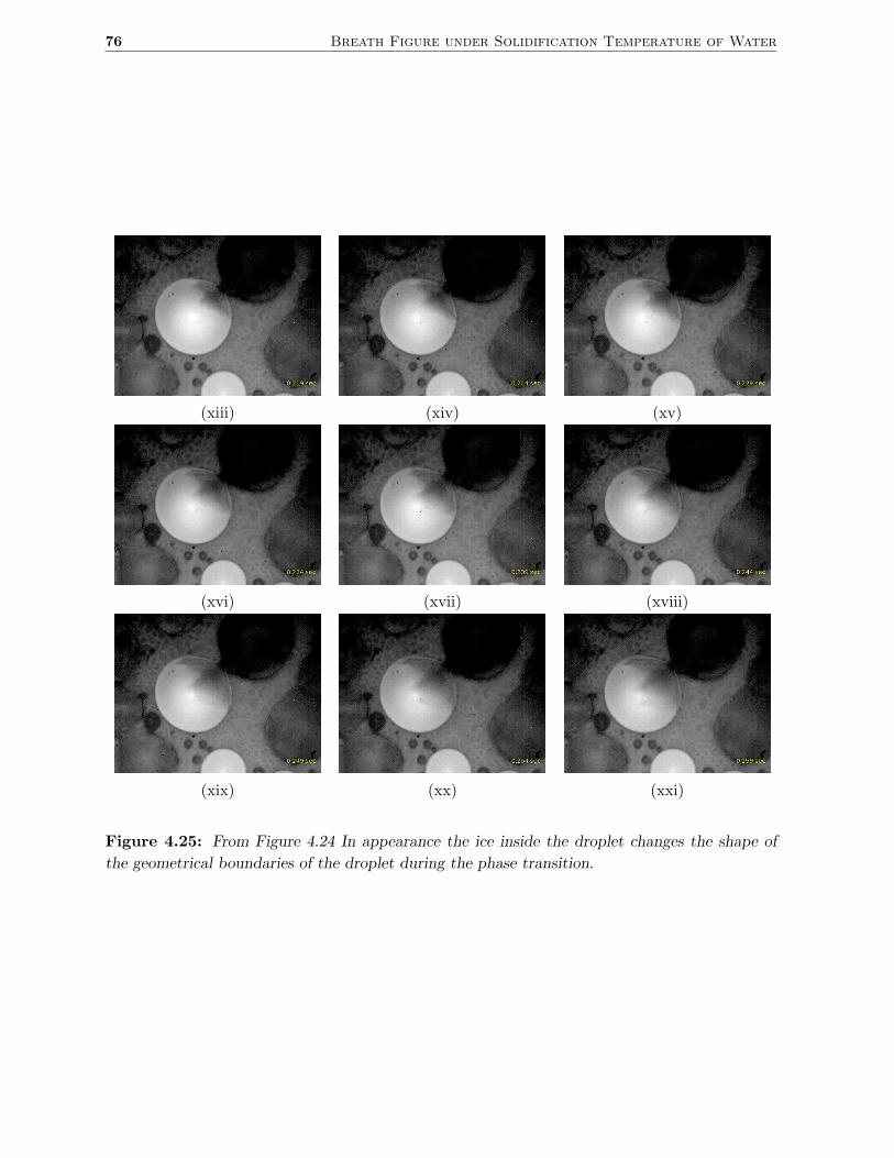
76 Breath Figure under Solidification Temperature of Water
(xiii) (xiv) (xv)
(xvi) (xvii) (xviii)
(xix) (xx) (xxi)
Figure 4.25: From Figure 4.24 In appearance the ice inside the droplet changes the shape of
the geometrical boundaries of the droplet during the phase transition.
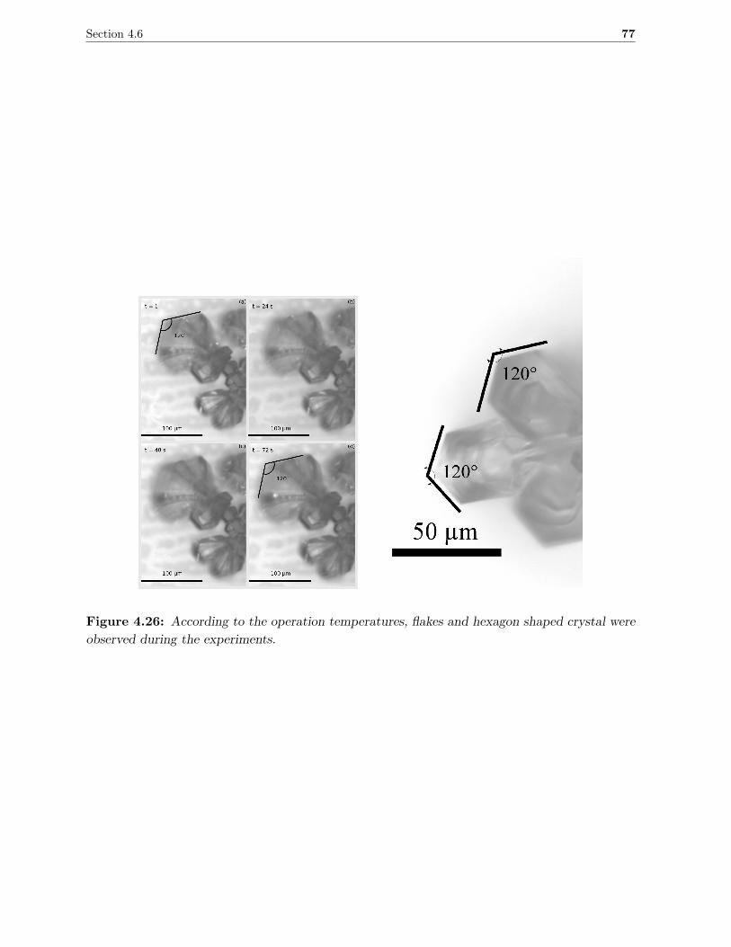
Section 4.6 77
Figure 4.26: According to the operation temperatures, flakes and hexagon shaped crystal were
observed during the experiments.

78 Breath Figure under Solidification Temperature of Water
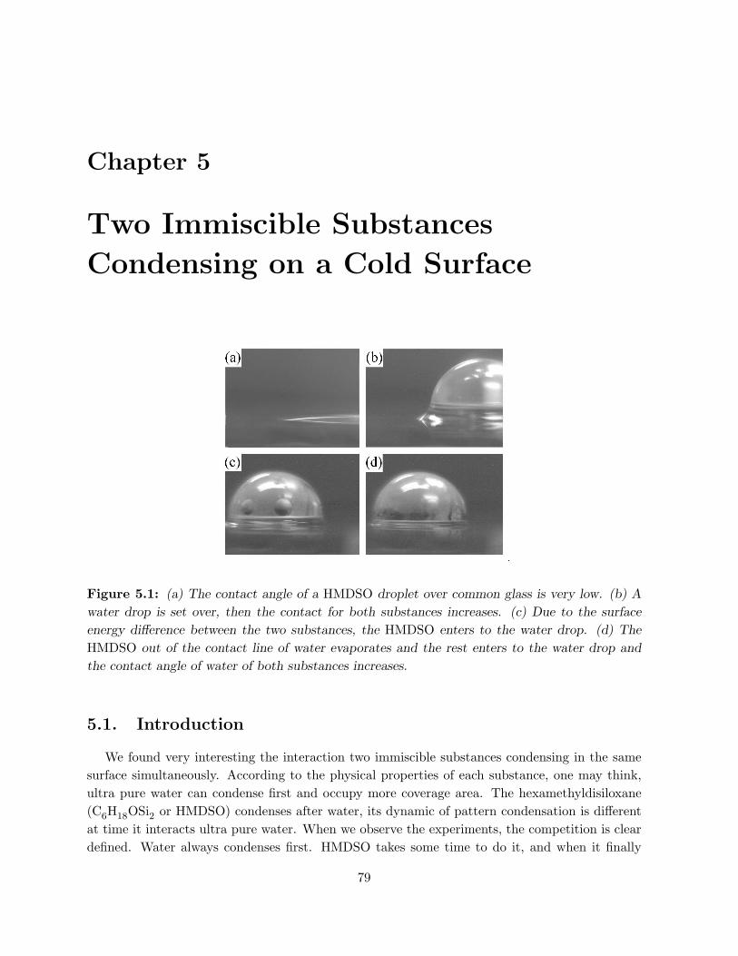
Chapter 5
Two Immiscible Substances
Condensing on a Cold Surface
Figure 5.1: (a) The contact angle of a HMDSO droplet over common glass is very low. (b) A
water drop is set over, then the contact for both substances increases. (c) Due to the surface
energy difference between the two substances, the HMDSO enters to the water drop. (d) The
HMDSO out of the contact line of water evaporates and the rest enters to the water drop and
the contact angle of water of both substances increases.
5.1. Introduction
We found very interesting the interaction two immiscible substances condensing in the same
surface simultaneously. According to the physical properties of each substance, one may think,
ultra pure water can condense first and occupy more coverage area. The hexamethyldisiloxane
(C6H18OSi2 or HMDSO) condenses after water, its dynamic of pattern condensation is different
at time it interacts ultra pure water. When we observe the experiments, the competition is clear
defined. Water always condenses first. HMDSO takes some time to do it, and when it finally
79
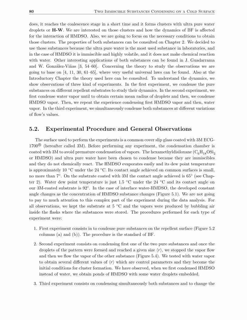
80 Two Immiscible Substances Condensing on a Cold Surface
does, it reaches the coalescence stage in a short time and it forms clusters with ultra pure water
droplets or H-W. We are interested on those clusters and how the dynamics of BF is affected
for the interaction of HMDSO. Also, we are going to focus on the necessary conditions to obtain
those clusters. The properties of both substances can be consulted on Chapter 2. We decided to
use those substances because the ultra pure water is the most used substance in laboratories, and
in the case of HMDSO it is immiscible and highly volatile, and it does not make chemical reaction
with water. Other interesting applications of both substances can be found in J. Guadarrama
and W. Gonzalez-Vinas [3, 54–60]. Concerning the theory to study the observations we are
going to base on [4, 11, 30, 61–65], where very useful universal laws can be found. Also at the
Introductory Chapter the theory used here can be consulted. To understand the dynamics, we
show observations of three kind of experiments. In the first experiment, we condense the pure
substances on different repellent substrates to study their dynamics. In the second experiment, we
first condense water vapor until to obtain certain mean radius of droplets and then, we condense
HMDSO vapor. Then, we repeat the experience condensing first HMDSO vapor and then, water
vapor. In the third experiment, we simultaneously condense both substances at different variations
of flow’s values.
5.2. Experimental Procedure and General Observations
The surface used to perform the experiments is a common cover slip glass coated with 3M ECG-
1700 R© (hereafter called 3M). Before performing any experiment, the condensation chamber is
coated with 3M to avoid premature condensation of vapors. The hexamethyldisiloxane (C6H18OSi2or HMDSO) and ultra pure water have been chosen to condense because they are immiscibles
and they do not chemically react. The HMDSO evaporates easily and its dew point temperature
is approximately 10 C under the 24 C. Its contact angle achieved on common surfaces is small,
no more than 7. On the substrate coated with 3M the contact angle achieved is 65 (see Chap-
ter 2). Water dew point temperature is just 1.5 C under the 24 C and its contact angle on
our 3M-coated substrate is 92. In the case of interface water-HMDSO, the developed constant
angle changes as the concentration of HMDSO substance changes (Figure 5.1). We are not going
to pay to much attention to this complex part of the experiment during the data analysis. For
all observations, we kept the substrate at 5 C and the vapors were produced by bubbling air
inside the flasks where the substances were stored. The procedures performed for each type of
experiment were:
1. First experiment consists in to condense pure substances on the repellent surface (Figure 5.2
columns (a) and (b)). The procedure is the standard of BF.
2. Second experiment consists on condensing first one of the two pure substances and once the
droplets of the pattern were formed and reached a given size 〈r〉, we stopped the vapor flow
and then we flow the vapor of the other substance (Figure 5.4). We tested with water vapor
to obtain several different values of 〈r〉 which are control parameters and they become the
initial conditions for cluster formation. We have observed, when we first condensed HMDSO
instead of water, we obtain ponds of HMDSO with some water droplets embedded.
3. Third experiment consists on condensing simultaneously both substances and to change the
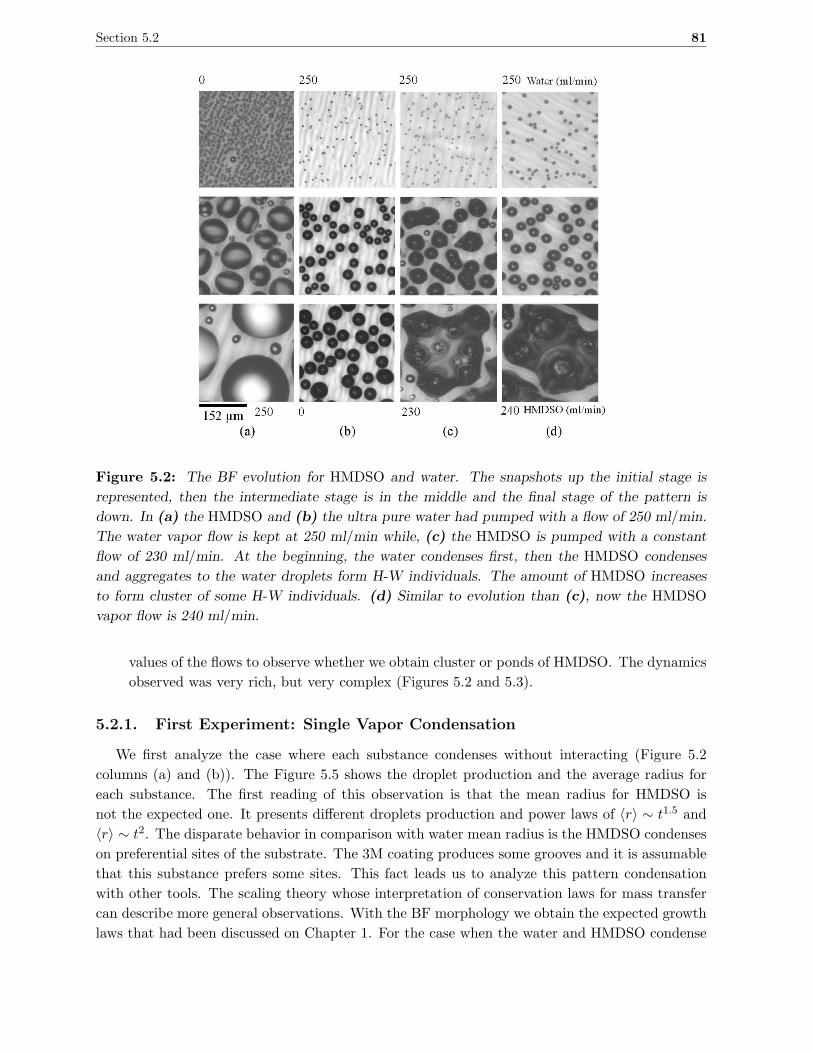
Section 5.2 81
Figure 5.2: The BF evolution for HMDSO and water. The snapshots up the initial stage is
represented, then the intermediate stage is in the middle and the final stage of the pattern is
down. In (a) the HMDSO and (b) the ultra pure water had pumped with a flow of 250 ml/min.
The water vapor flow is kept at 250 ml/min while, (c) the HMDSO is pumped with a constant
flow of 230 ml/min. At the beginning, the water condenses first, then the HMDSO condenses
and aggregates to the water droplets form H-W individuals. The amount of HMDSO increases
to form cluster of some H-W individuals. (d) Similar to evolution than (c), now the HMDSO
vapor flow is 240 ml/min.
values of the flows to observe whether we obtain cluster or ponds of HMDSO. The dynamics
observed was very rich, but very complex (Figures 5.2 and 5.3).
5.2.1. First Experiment: Single Vapor Condensation
We first analyze the case where each substance condenses without interacting (Figure 5.2
columns (a) and (b)). The Figure 5.5 shows the droplet production and the average radius for
each substance. The first reading of this observation is that the mean radius for HMDSO is
not the expected one. It presents different droplets production and power laws of 〈r〉 ∼ t1.5 and
〈r〉 ∼ t2. The disparate behavior in comparison with water mean radius is the HMDSO condenses
on preferential sites of the substrate. The 3M coating produces some grooves and it is assumable
that this substance prefers some sites. This fact leads us to analyze this pattern condensation
with other tools. The scaling theory whose interpretation of conservation laws for mass transfer
can describe more general observations. With the BF morphology we obtain the expected growth
laws that had been discussed on Chapter 1. For the case when the water and HMDSO condense
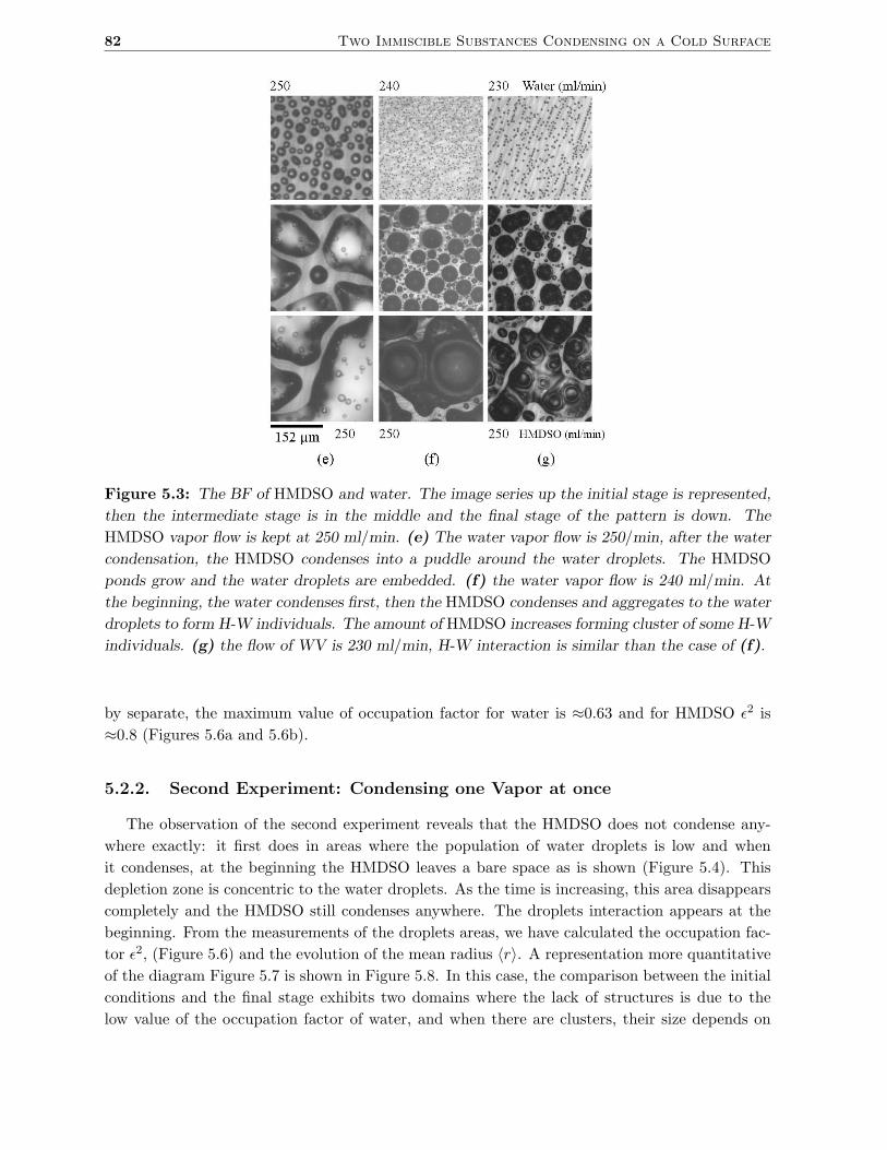
82 Two Immiscible Substances Condensing on a Cold Surface
Figure 5.3: The BF of HMDSO and water. The image series up the initial stage is represented,
then the intermediate stage is in the middle and the final stage of the pattern is down. The
HMDSO vapor flow is kept at 250 ml/min. (e) The water vapor flow is 250/min, after the water
condensation, the HMDSO condenses into a puddle around the water droplets. The HMDSO
ponds grow and the water droplets are embedded. (f) the water vapor flow is 240 ml/min. At
the beginning, the water condenses first, then the HMDSO condenses and aggregates to the water
droplets to form H-W individuals. The amount of HMDSO increases forming cluster of some H-W
individuals. (g) the flow of WV is 230 ml/min, H-W interaction is similar than the case of (f).
by separate, the maximum value of occupation factor for water is ≈0.63 and for HMDSO ǫ2 is
≈0.8 (Figures 5.6a and 5.6b).
5.2.2. Second Experiment: Condensing one Vapor at once
The observation of the second experiment reveals that the HMDSO does not condense any-
where exactly: it first does in areas where the population of water droplets is low and when
it condenses, at the beginning the HMDSO leaves a bare space as is shown (Figure 5.4). This
depletion zone is concentric to the water droplets. As the time is increasing, this area disappears
completely and the HMDSO still condenses anywhere. The droplets interaction appears at the
beginning. From the measurements of the droplets areas, we have calculated the occupation fac-
tor ǫ2, (Figure 5.6) and the evolution of the mean radius 〈r〉. A representation more quantitative
of the diagram Figure 5.7 is shown in Figure 5.8. In this case, the comparison between the initial
conditions and the final stage exhibits two domains where the lack of structures is due to the
low value of the occupation factor of water, and when there are clusters, their size depends on
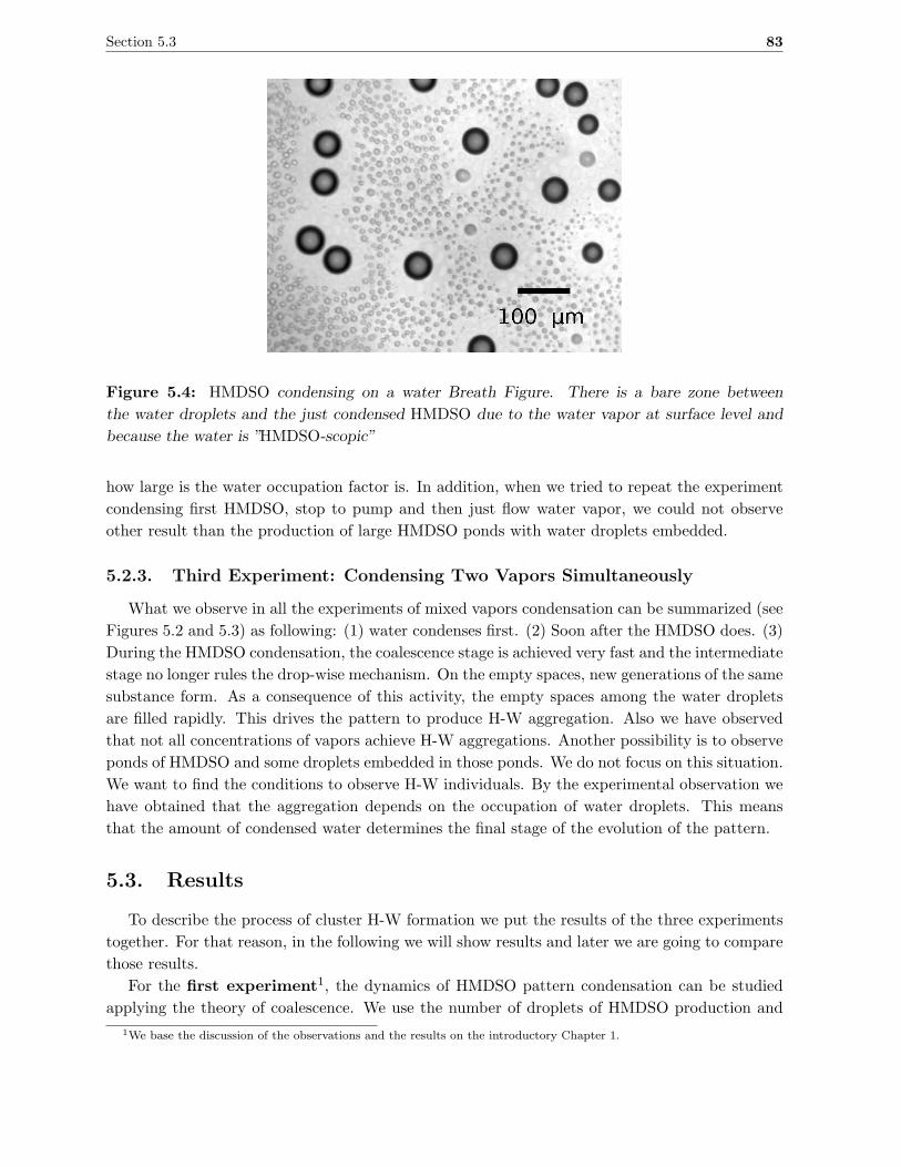
Section 5.3 83
Figure 5.4: HMDSO condensing on a water Breath Figure. There is a bare zone between
the water droplets and the just condensed HMDSO due to the water vapor at surface level and
because the water is ”HMDSO-scopic”
how large is the water occupation factor is. In addition, when we tried to repeat the experiment
condensing first HMDSO, stop to pump and then just flow water vapor, we could not observe
other result than the production of large HMDSO ponds with water droplets embedded.
5.2.3. Third Experiment: Condensing Two Vapors Simultaneously
What we observe in all the experiments of mixed vapors condensation can be summarized (see
Figures 5.2 and 5.3) as following: (1) water condenses first. (2) Soon after the HMDSO does. (3)
During the HMDSO condensation, the coalescence stage is achieved very fast and the intermediate
stage no longer rules the drop-wise mechanism. On the empty spaces, new generations of the same
substance form. As a consequence of this activity, the empty spaces among the water droplets
are filled rapidly. This drives the pattern to produce H-W aggregation. Also we have observed
that not all concentrations of vapors achieve H-W aggregations. Another possibility is to observe
ponds of HMDSO and some droplets embedded in those ponds. We do not focus on this situation.
We want to find the conditions to observe H-W individuals. By the experimental observation we
have obtained that the aggregation depends on the occupation of water droplets. This means
that the amount of condensed water determines the final stage of the evolution of the pattern.
5.3. Results
To describe the process of cluster H-W formation we put the results of the three experiments
together. For that reason, in the following we will show results and later we are going to compare
those results.
For the first experiment1, the dynamics of HMDSO pattern condensation can be studied
applying the theory of coalescence. We use the number of droplets of HMDSO production and
1We base the discussion of the observations and the results on the introductory Chapter 1.
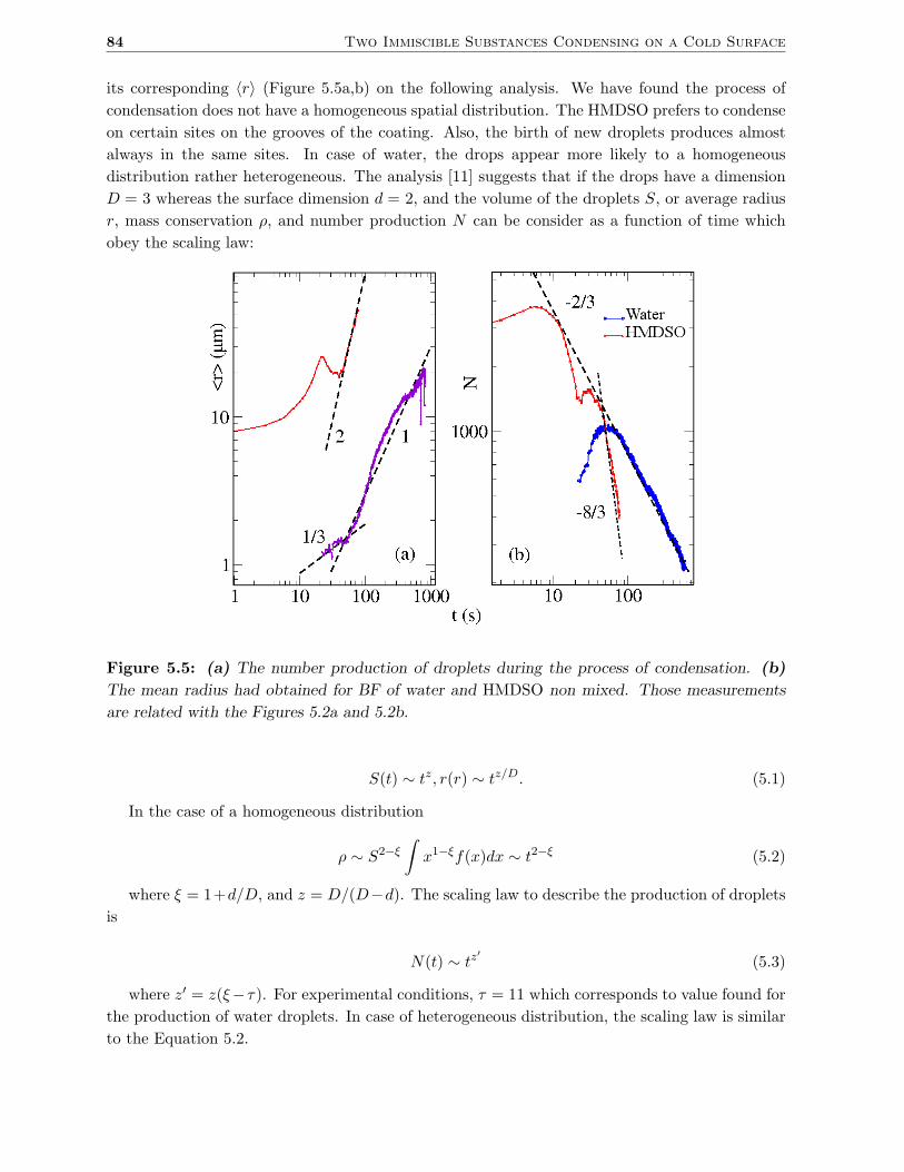
84 Two Immiscible Substances Condensing on a Cold Surface
its corresponding 〈r〉 (Figure 5.5a,b) on the following analysis. We have found the process of
condensation does not have a homogeneous spatial distribution. The HMDSO prefers to condense
on certain sites on the grooves of the coating. Also, the birth of new droplets produces almost
always in the same sites. In case of water, the drops appear more likely to a homogeneous
distribution rather heterogeneous. The analysis [11] suggests that if the drops have a dimension
D = 3 whereas the surface dimension d = 2, and the volume of the droplets S, or average radius
r, mass conservation ρ, and number production N can be consider as a function of time which
obey the scaling law:
Figure 5.5: (a) The number production of droplets during the process of condensation. (b)
The mean radius had obtained for BF of water and HMDSO non mixed. Those measurements
are related with the Figures 5.2a and 5.2b.
S(t) ∼ tz, r(r) ∼ tz/D. (5.1)
In the case of a homogeneous distribution
ρ ∼ S2−ξ
∫
x1−ξf(x)dx ∼ t2−ξ (5.2)
where ξ = 1+d/D, and z = D/(D−d). The scaling law to describe the production of droplets
is
N(t) ∼ tz′
(5.3)
where z′ = z(ξ−τ). For experimental conditions, τ = 11 which corresponds to value found for
the production of water droplets. In case of heterogeneous distribution, the scaling law is similar
to the Equation 5.2.
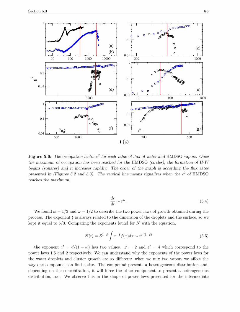
Section 5.3 85
Figure 5.6: The occupation factor ǫ2 for each value of flux of water and HMDSO vapors. Once
the maximum of occupation has been reached for the HMDSO (circles), the formation of H-W
begins (squares) and it increases rapidly. The order of the graph is according the flux rates
presented in (Figures 5.2 and 5.3). The vertical line means signalizes when the ǫ2 of HMDSO
reaches the maximum.
dr
dt∼ rω. (5.4)
We found ω = 1/3 and ω = 1/2 to describe the two power laws of growth obtained during the
process. The exponent ξ is always related to the dimension of the droplets and the surface, so we
kept it equal to 5/3. Comparing the exponents found for N with the equation,
N(t) = S1−ξ
∫
x−ξf(x)dx ∼ tz′(1−ξ) (5.5)
the exponent z′ = d/(1 − ω) has two values. z′ = 2 and z′ = 4 which correspond to the
power laws 1.5 and 2 respectively. We can understand why the exponents of the power laws for
the water droplets and cluster growth are so different: when we mix two vapors we affect the
way one compound can find a site. The compound presents a heterogeneous distribution and,
depending on the concentration, it will force the other component to present a heterogeneous
distribution, too. We observe this in the shape of power laws presented for the intermediate
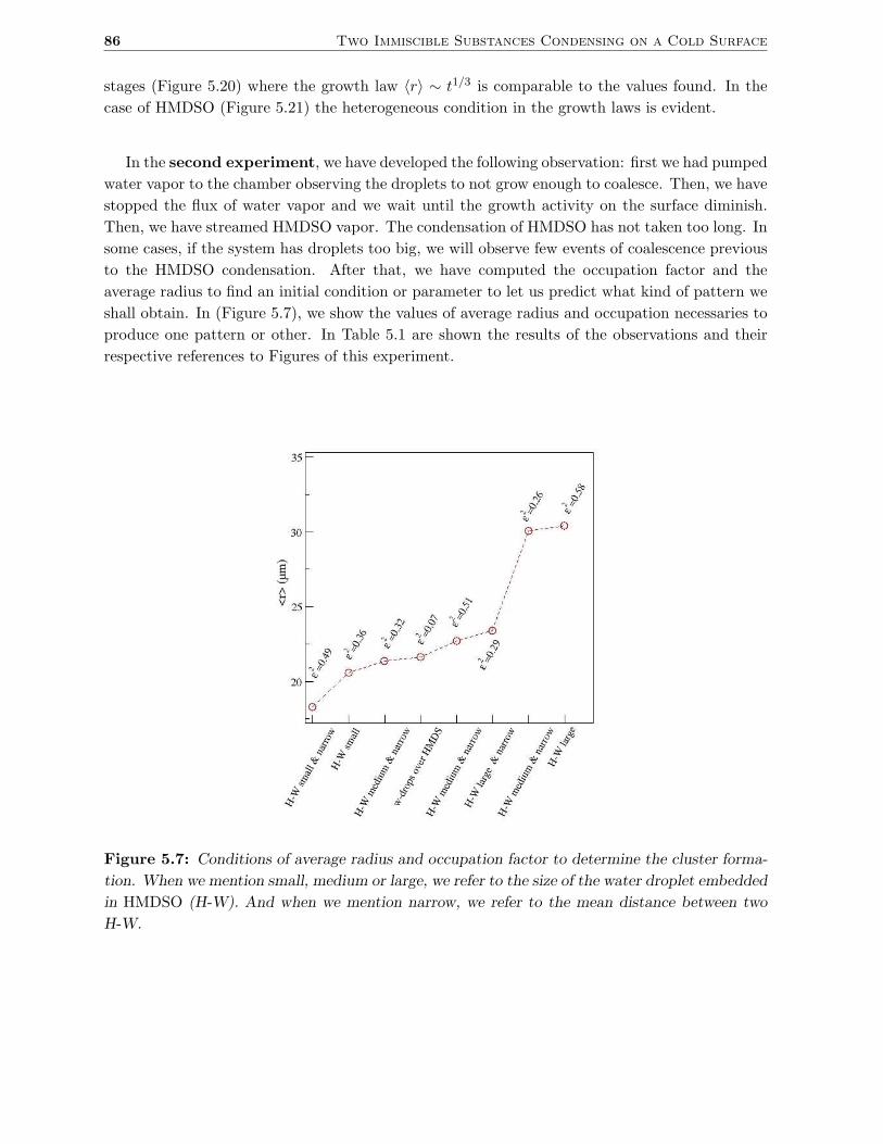
86 Two Immiscible Substances Condensing on a Cold Surface
stages (Figure 5.20) where the growth law 〈r〉 ∼ t1/3 is comparable to the values found. In the
case of HMDSO (Figure 5.21) the heterogeneous condition in the growth laws is evident.
In the second experiment, we have developed the following observation: first we had pumped
water vapor to the chamber observing the droplets to not grow enough to coalesce. Then, we have
stopped the flux of water vapor and we wait until the growth activity on the surface diminish.
Then, we have streamed HMDSO vapor. The condensation of HMDSO has not taken too long. In
some cases, if the system has droplets too big, we will observe few events of coalescence previous
to the HMDSO condensation. After that, we have computed the occupation factor and the
average radius to find an initial condition or parameter to let us predict what kind of pattern we
shall obtain. In (Figure 5.7), we show the values of average radius and occupation necessaries to
produce one pattern or other. In Table 5.1 are shown the results of the observations and their
respective references to Figures of this experiment.
Figure 5.7: Conditions of average radius and occupation factor to determine the cluster forma-
tion. When we mention small, medium or large, we refer to the size of the water droplet embedded
in HMDSO (H-W). And when we mention narrow, we refer to the mean distance between two
H-W.
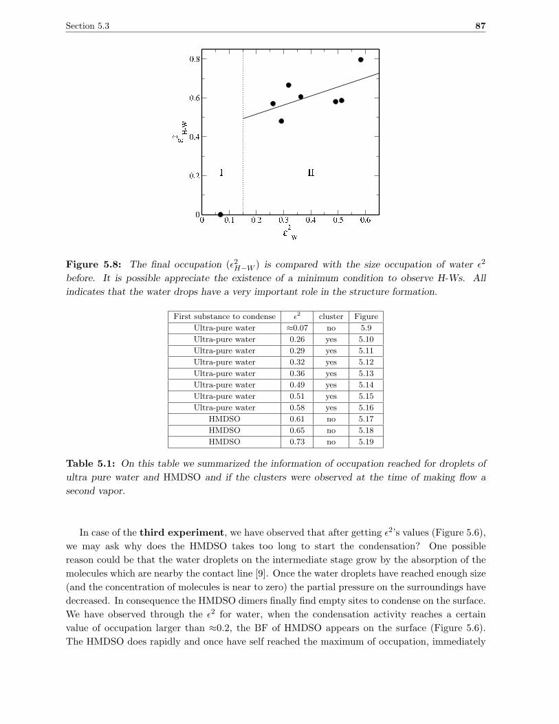
Section 5.3 87
0 0 0 0 0 0 0
e2
W
0
0
0
0
0
H
Figure 5.8: The final occupation (ǫ2H−W ) is compared with the size occupation of water ǫ2
before. It is possible appreciate the existence of a minimum condition to observe H-Ws. All
indicates that the water drops have a very important role in the structure formation.
First substance to condense ǫ2 cluster Figure
Ultra-pure water ≈0.07 no 5.9
Ultra-pure water 0.26 yes 5.10
Ultra-pure water 0.29 yes 5.11
Ultra-pure water 0.32 yes 5.12
Ultra-pure water 0.36 yes 5.13
Ultra-pure water 0.49 yes 5.14
Ultra-pure water 0.51 yes 5.15
Ultra-pure water 0.58 yes 5.16
HMDSO 0.61 no 5.17
HMDSO 0.65 no 5.18
HMDSO 0.73 no 5.19
Table 5.1: On this table we summarized the information of occupation reached for droplets of
ultra pure water and HMDSO and if the clusters were observed at the time of making flow a
second vapor.
In case of the third experiment, we have observed that after getting ǫ2’s values (Figure 5.6),
we may ask why does the HMDSO takes too long to start the condensation? One possible
reason could be that the water droplets on the intermediate stage grow by the absorption of the
molecules which are nearby the contact line [9]. Once the water droplets have reached enough size
(and the concentration of molecules is near to zero) the partial pressure on the surroundings have
decreased. In consequence the HMDSO dimers finally find empty sites to condense on the surface.
We have observed through the ǫ2 for water, when the condensation activity reaches a certain
value of occupation larger than ≈0.2, the BF of HMDSO appears on the surface (Figure 5.6).
The HMDSO does rapidly and once have self reached the maximum of occupation, immediately
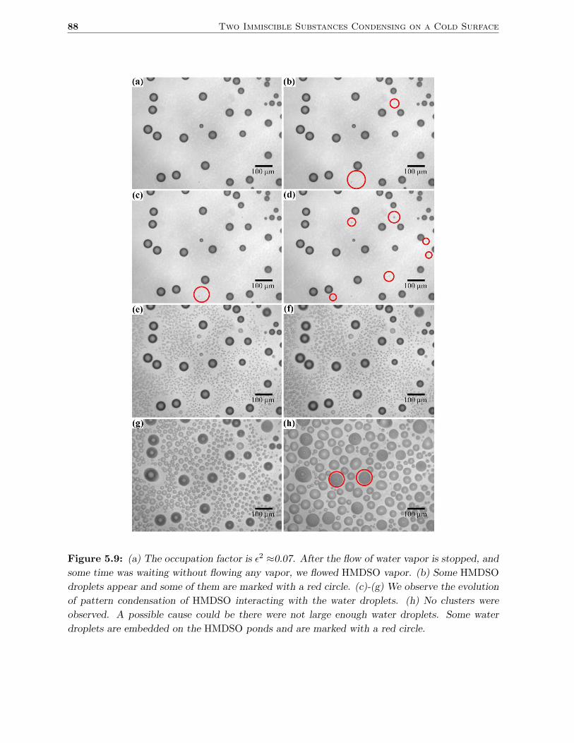
88 Two Immiscible Substances Condensing on a Cold Surface
Figure 5.9: (a) The occupation factor is ǫ2 ≈0.07. After the flow of water vapor is stopped, and
some time was waiting without flowing any vapor, we flowed HMDSO vapor. (b) Some HMDSO
droplets appear and some of them are marked with a red circle. (c)-(g) We observe the evolution
of pattern condensation of HMDSO interacting with the water droplets. (h) No clusters were
observed. A possible cause could be there were not large enough water droplets. Some water
droplets are embedded on the HMDSO ponds and are marked with a red circle.
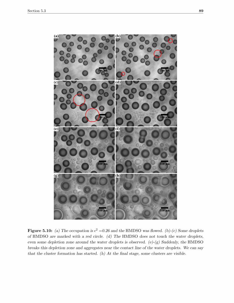
Section 5.3 89
Figure 5.10: (a) The occupation is ǫ2 =0.26 and the HMDSO was flowed. (b)-(c) Some droplets
of HMDSO are marked with a red circle. (d) The HMDSO does not touch the water droplets,
even some depletion zone around the water droplets is observed. (e)-(g) Suddenly, the HMDSO
breaks this depletion zone and aggregates near the contact line of the water droplets. We can say
that the cluster formation has started. (h) At the final stage, some clusters are visible.
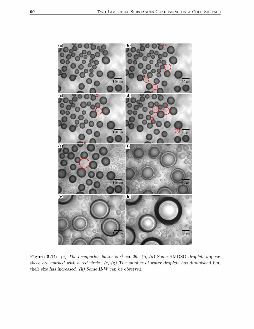
90 Two Immiscible Substances Condensing on a Cold Surface
Figure 5.11: (a) The occupation factor is ǫ2 =0.29. (b)-(d) Some HMDSO droplets appear,
those are marked with a red circle. (e)-(g) The number of water droplets has diminished but,
their size has increased. (h) Some H-W can be observed.
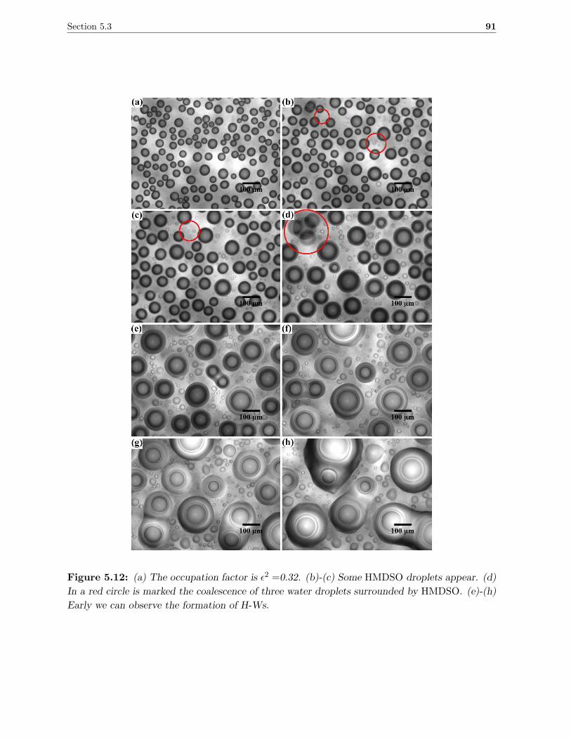
Section 5.3 91
Figure 5.12: (a) The occupation factor is ǫ2 =0.32. (b)-(c) Some HMDSO droplets appear. (d)
In a red circle is marked the coalescence of three water droplets surrounded by HMDSO. (e)-(h)
Early we can observe the formation of H-Ws.
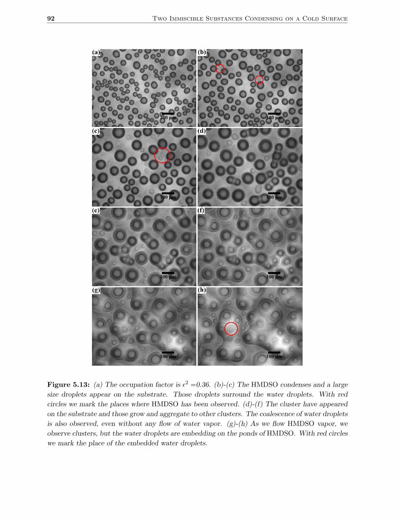
92 Two Immiscible Substances Condensing on a Cold Surface
Figure 5.13: (a) The occupation factor is ǫ2 =0.36. (b)-(c) The HMDSO condenses and a large
size droplets appear on the substrate. Those droplets surround the water droplets. With red
circles we mark the places where HMDSO has been observed. (d)-(f) The cluster have appeared
on the substrate and those grow and aggregate to other clusters. The coalescence of water droplets
is also observed, even without any flow of water vapor. (g)-(h) As we flow HMDSO vapor, we
observe clusters, but the water droplets are embedding on the ponds of HMDSO. With red circles
we mark the place of the embedded water droplets.
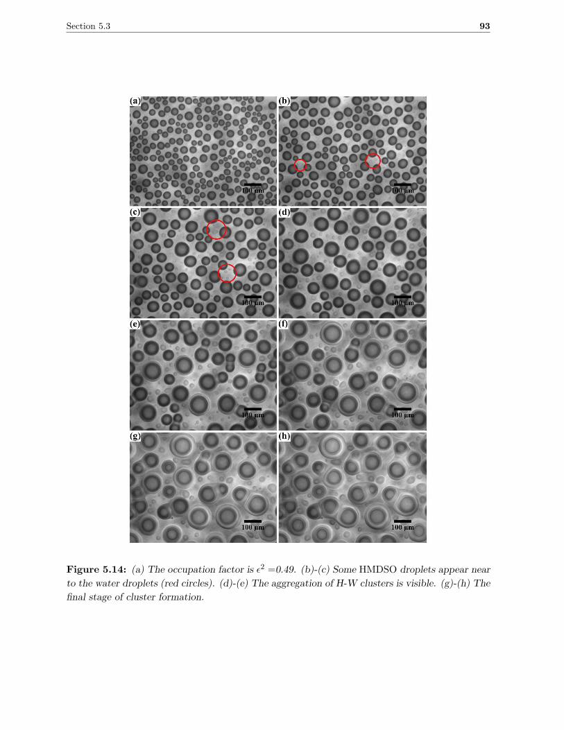
Section 5.3 93
Figure 5.14: (a) The occupation factor is ǫ2 =0.49. (b)-(c) Some HMDSO droplets appear near
to the water droplets (red circles). (d)-(e) The aggregation of H-W clusters is visible. (g)-(h) The
final stage of cluster formation.
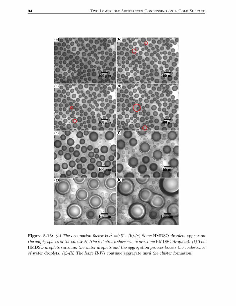
94 Two Immiscible Substances Condensing on a Cold Surface
Figure 5.15: (a) The occupation factor is ǫ2 =0.51. (b)-(e) Some HMDSO droplets appear on
the empty spaces of the substrate (the red circles show where are some HMDSO droplets). (f) The
HMDSO droplets surround the water droplets and the aggregation process boosts the coalescence
of water droplets. (g)-(h) The large H-Ws continue aggregate until the cluster formation.
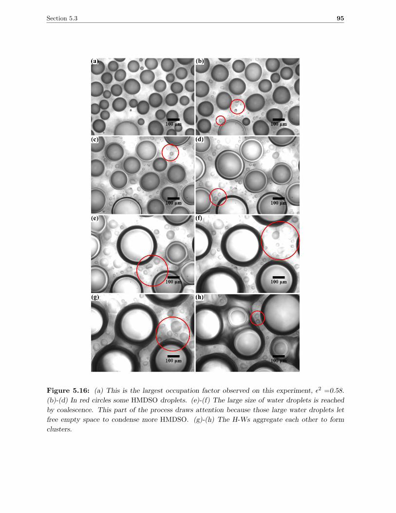
Section 5.3 95
Figure 5.16: (a) This is the largest occupation factor observed on this experiment, ǫ2 =0.58.
(b)-(d) In red circles some HMDSO droplets. (e)-(f) The large size of water droplets is reached
by coalescence. This part of the process draws attention because those large water droplets let
free empty space to condense more HMDSO. (g)-(h) The H-Ws aggregate each other to form
clusters.
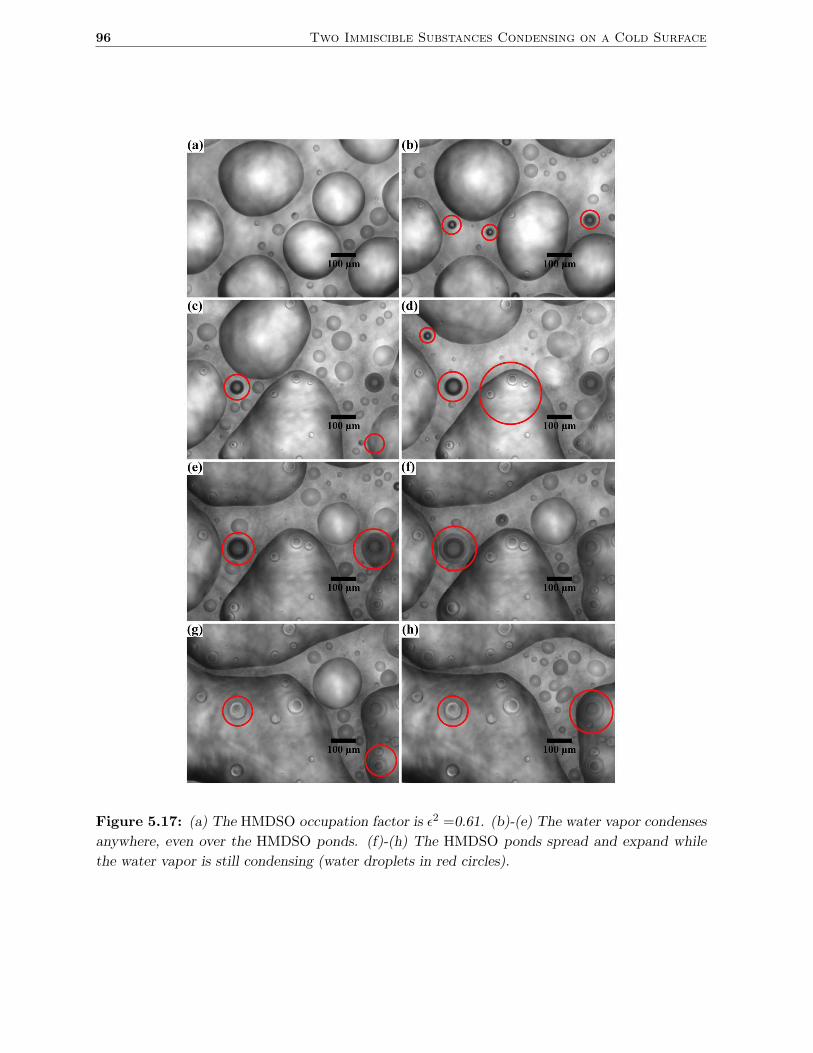
96 Two Immiscible Substances Condensing on a Cold Surface
Figure 5.17: (a) The HMDSO occupation factor is ǫ2 =0.61. (b)-(e) The water vapor condenses
anywhere, even over the HMDSO ponds. (f)-(h) The HMDSO ponds spread and expand while
the water vapor is still condensing (water droplets in red circles).
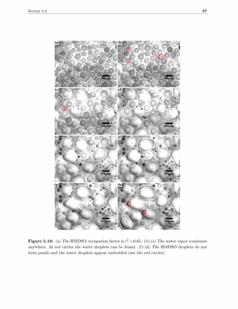
Section 5.3 97
Figure 5.18: (a) The HMDSO occupation factor is ǫ2 =0.65. (b)-(e) The water vapor condenses
anywhere. In red circles the water droplets can be found. (f)-(h) The HMDSO droplets do not
form ponds and the water droplets appear embedded (see the red circles).
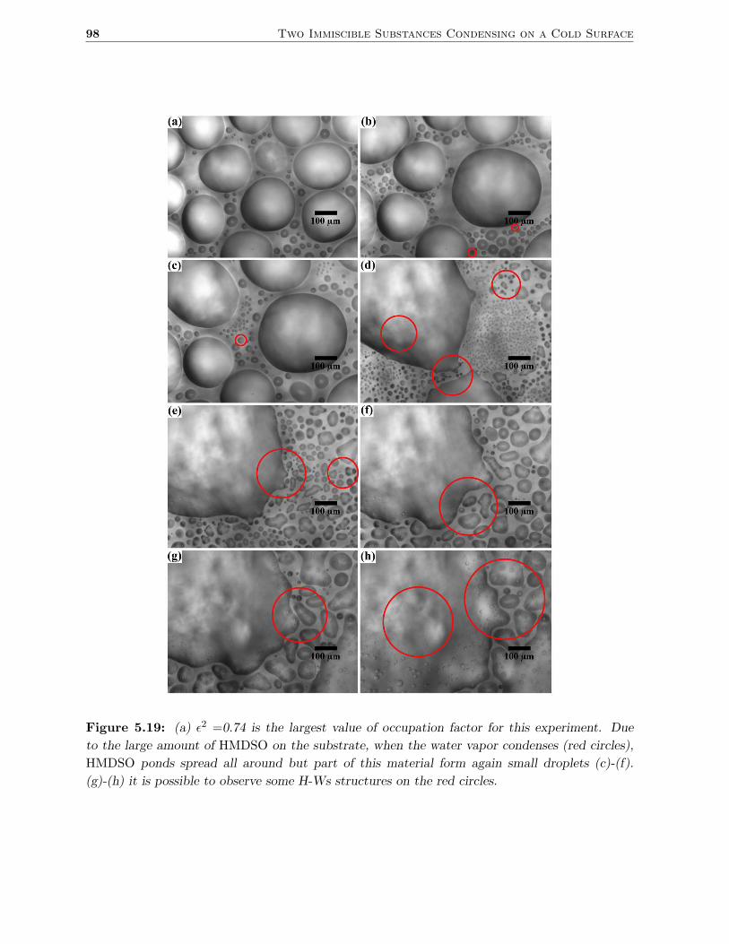
98 Two Immiscible Substances Condensing on a Cold Surface
Figure 5.19: (a) ǫ2 =0.74 is the largest value of occupation factor for this experiment. Due
to the large amount of HMDSO on the substrate, when the water vapor condenses (red circles),
HMDSO ponds spread all around but part of this material form again small droplets (c)-(f).
(g)-(h) it is possible to observe some H-Ws structures on the red circles.
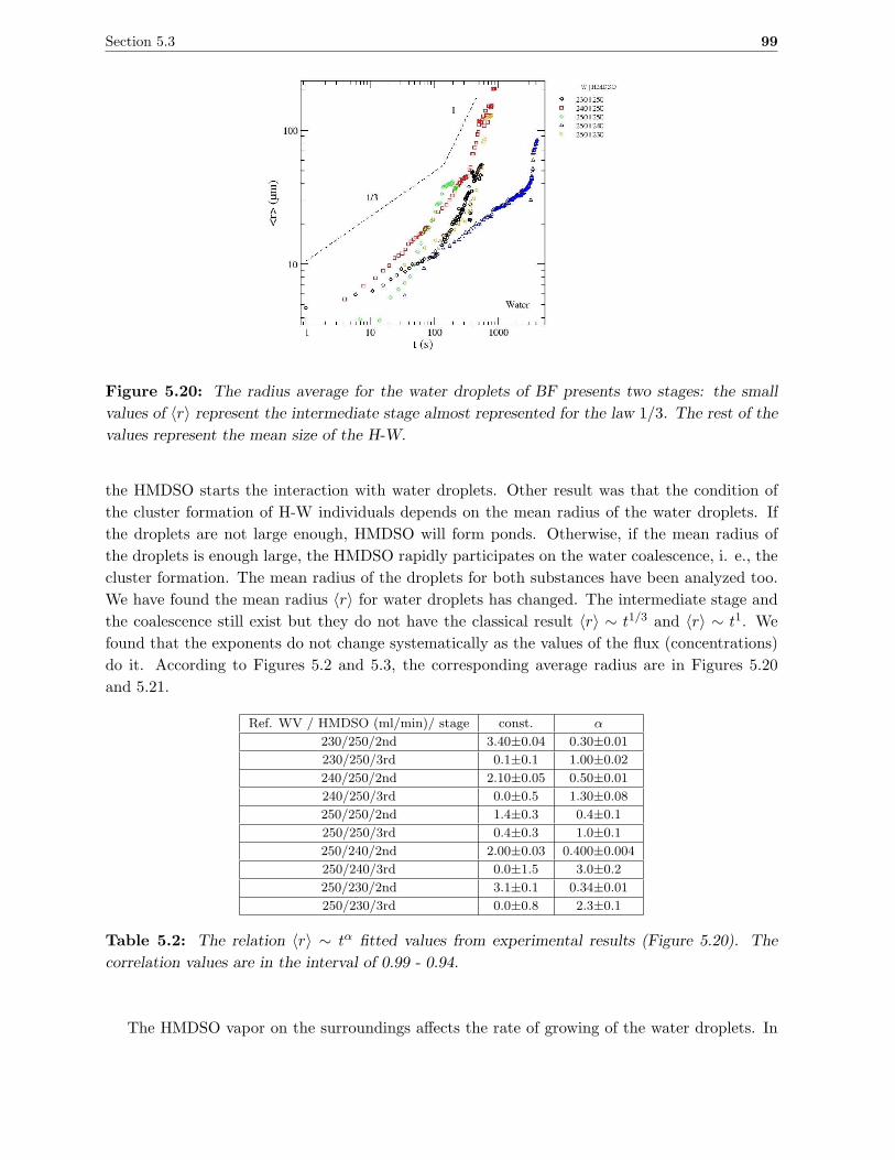
Section 5.3 99
Figure 5.20: The radius average for the water droplets of BF presents two stages: the small
values of 〈r〉 represent the intermediate stage almost represented for the law 1/3. The rest of the
values represent the mean size of the H-W.
the HMDSO starts the interaction with water droplets. Other result was that the condition of
the cluster formation of H-W individuals depends on the mean radius of the water droplets. If
the droplets are not large enough, HMDSO will form ponds. Otherwise, if the mean radius of
the droplets is enough large, the HMDSO rapidly participates on the water coalescence, i. e., the
cluster formation. The mean radius of the droplets for both substances have been analyzed too.
We have found the mean radius 〈r〉 for water droplets has changed. The intermediate stage and
the coalescence still exist but they do not have the classical result 〈r〉 ∼ t1/3 and 〈r〉 ∼ t1. We
found that the exponents do not change systematically as the values of the flux (concentrations)
do it. According to Figures 5.2 and 5.3, the corresponding average radius are in Figures 5.20
and 5.21.
Ref. WV / HMDSO (ml/min)/ stage const. α
230/250/2nd 3.40±0.04 0.30±0.01
230/250/3rd 0.1±0.1 1.00±0.02
240/250/2nd 2.10±0.05 0.50±0.01
240/250/3rd 0.0±0.5 1.30±0.08
250/250/2nd 1.4±0.3 0.4±0.1
250/250/3rd 0.4±0.3 1.0±0.1
250/240/2nd 2.00±0.03 0.400±0.004
250/240/3rd 0.0±1.5 3.0±0.2
250/230/2nd 3.1±0.1 0.34±0.01
250/230/3rd 0.0±0.8 2.3±0.1
Table 5.2: The relation 〈r〉 ∼ tα fitted values from experimental results (Figure 5.20). The
correlation values are in the interval of 0.99 - 0.94.
The HMDSO vapor on the surroundings affects the rate of growing of the water droplets. In
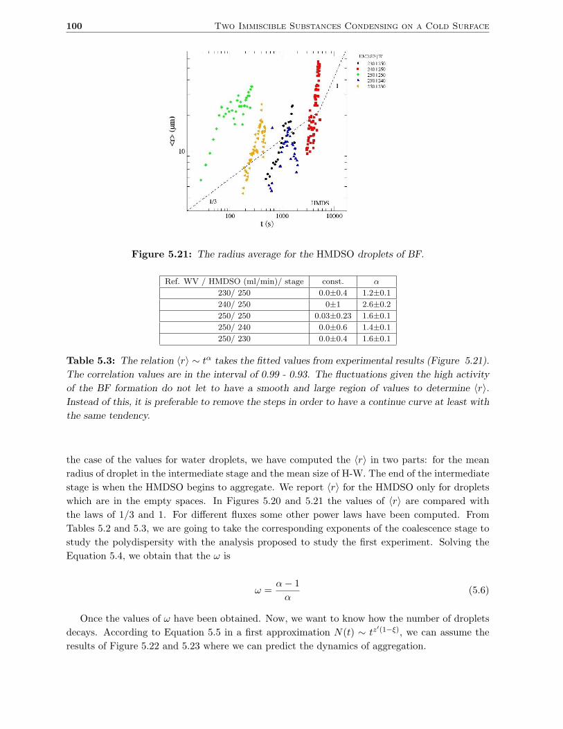
100 Two Immiscible Substances Condensing on a Cold Surface
Figure 5.21: The radius average for the HMDSO droplets of BF.
Ref. WV / HMDSO (ml/min)/ stage const. α
230/ 250 0.0±0.4 1.2±0.1
240/ 250 0±1 2.6±0.2
250/ 250 0.03±0.23 1.6±0.1
250/ 240 0.0±0.6 1.4±0.1
250/ 230 0.0±0.4 1.6±0.1
Table 5.3: The relation 〈r〉 ∼ tα takes the fitted values from experimental results (Figure 5.21).
The correlation values are in the interval of 0.99 - 0.93. The fluctuations given the high activity
of the BF formation do not let to have a smooth and large region of values to determine 〈r〉.
Instead of this, it is preferable to remove the steps in order to have a continue curve at least with
the same tendency.
the case of the values for water droplets, we have computed the 〈r〉 in two parts: for the mean
radius of droplet in the intermediate stage and the mean size of H-W. The end of the intermediate
stage is when the HMDSO begins to aggregate. We report 〈r〉 for the HMDSO only for droplets
which are in the empty spaces. In Figures 5.20 and 5.21 the values of 〈r〉 are compared with
the laws of 1/3 and 1. For different fluxes some other power laws have been computed. From
Tables 5.2 and 5.3, we are going to take the corresponding exponents of the coalescence stage to
study the polydispersity with the analysis proposed to study the first experiment. Solving the
Equation 5.4, we obtain that the ω is
ω =α− 1
α(5.6)
Once the values of ω have been obtained. Now, we want to know how the number of droplets
decays. According to Equation 5.5 in a first approximation N(t) ∼ tz′(1−ξ), we can assume the
results of Figure 5.22 and 5.23 where we can predict the dynamics of aggregation.
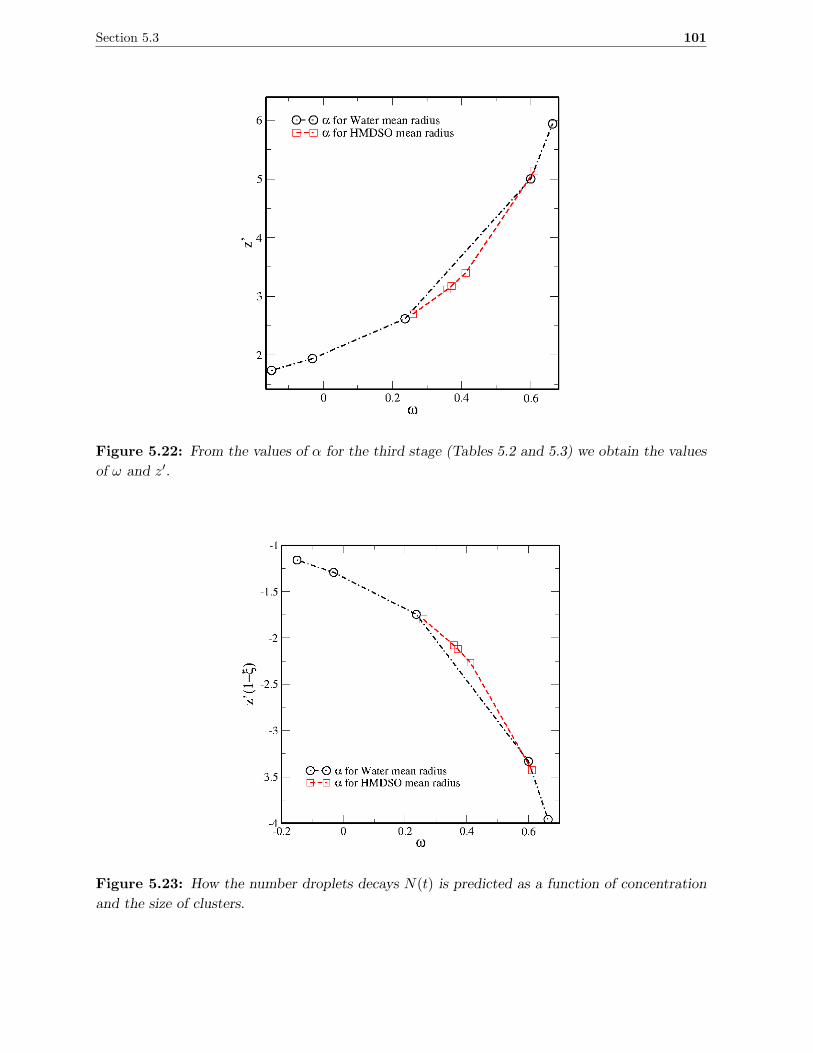
Section 5.3 101
Figure 5.22: From the values of α for the third stage (Tables 5.2 and 5.3) we obtain the values
of ω and z′.
Figure 5.23: How the number droplets decays N(t) is predicted as a function of concentration
and the size of clusters.
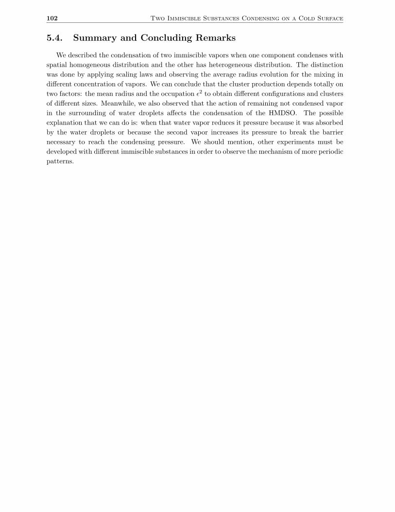
102 Two Immiscible Substances Condensing on a Cold Surface
5.4. Summary and Concluding Remarks
We described the condensation of two immiscible vapors when one component condenses with
spatial homogeneous distribution and the other has heterogeneous distribution. The distinction
was done by applying scaling laws and observing the average radius evolution for the mixing in
different concentration of vapors. We can conclude that the cluster production depends totally on
two factors: the mean radius and the occupation ǫ2 to obtain different configurations and clusters
of different sizes. Meanwhile, we also observed that the action of remaining not condensed vapor
in the surrounding of water droplets affects the condensation of the HMDSO. The possible
explanation that we can do is: when that water vapor reduces it pressure because it was absorbed
by the water droplets or because the second vapor increases its pressure to break the barrier
necessary to reach the condensing pressure. We should mention, other experiments must be
developed with different immiscible substances in order to observe the mechanism of more periodic
patterns.
Conclusions and Outlook
Conclusions
BF phenomena are ruled by several parameters. The most important variables are the tem-
perature, pressure, surface tension, vapor saturation and hydrodynamic flows. At microscopic
level, the interaction of molecules of vapor with defects on the surface also affects the contact
angle of droplets. However, other parameters related with chemical potentials and bounds can be
involved on the dynamics, like in the case of ice propagation. At the laboratory, we controlled the
temperature, the flow of vapors, and the liquid-solid contact angle. We could measure the radii
of drops. We characterized the dynamics when the BF is in a presence of a humidity sink (Chap-
ter 2). Because the humidity sink has a radial geometry, we suggest the Fick’s law J = −D∇n in
radial coordinates is the solution for the molecules’ flux. Through the mathematical solution, we
studied the relation between the water vapor flowed to the chamber and the time crossing of the
depletion zone and the radius of the salty drop. This attempt helps us to depict the pressure
gradient within the depletion zone and the singularities produced by the BF pattern and the
salty drop’s perimeter. This latter result is a clue to know the saturation pressure of vapor in the
surroundings of BF. In brief, the conclusions can be summarized as:
1. The depletion zone exists because there the vapor is not supersaturated and it cannot con-
dense.
2. The width of the depletion zone δ could be described as a solution of Bessel’s polynomials
and exponential function using the value of the radius of a sink R. This result lead us to
set a model of condensation to understand the depletion zone around the salty drop. This
model allows to compute the profile of the pressure in the depletion zone.
The relevance of the BF (with ultra-pure water) on frost formation and propagation of ice was
discovered during experiments (Chapter 4). The classical description of 〈r〉 ∼ t1/3 is also valid and
applicable for the intermediate stage of supercooled water droplets. The recognition of the phase
transition from liquid into solid is done through ǫ2. The phenomenology is very rich in physical
processes like the coexistence and interaction between solid, gas and liquid phases of water. Those
interactions can be classified into percolation and deposition. The process of evaporation through
dm/dt ∼ dR3/dt obeys the law R(t)2 = R20 − tα where R0 is the initial radius of two droplets
separated by a distance d0. Those results were corroborated with the experimental measurements.
The velocity of propagation is measured as the dendrites growth at expense of water droplets.
From those measurements it is possible to describe the conditions of minimum droplet’s radius
and critical time for the percolation process to exist. In other experiments performed at the same
103
104 Conclusions and Outlook
conditions, we studied also the anisotropy of water vapor condensation and the adsorption by
a humidity sink. We found how is the impact on the adsorption process when the BF pattern
is homogeneous or not. In this way, it is left to work on the theoretical explanations and more
controlled experiments.
We described the condensation of two immiscible vapors when one component condenses with
spatial homogeneous distribution and the other has heterogeneous distribution. The distinction
was done applying scaling laws and observing the average radius evolution for the mixing in
different concentration of vapors. We can conclude that the cluster production depends totally
on two factors: the mean radius and the occupation ǫ2 to obtain different configurations and
clusters of different sizes. Meanwhile, we also observed that the action of remaining vapor in the
surrounding of water droplets affects the condensation of the HMDSO. We can explain that the
water vapor reduces its pressure because it is adsorbed by the water droplets (the second vapor
increases its pressure to break the barrier necessary to reach the supersaturation pressure).
Outlook
Two branches of research can grow from this thesis work. The first one, is the field of the
hydrodynamics and microfluidics to study complex flux inside the condensation chamber with
walls at different temperatures in order to have forced convection, other work can be the study
of the vapor flow just in the interface liquid gas of the drops. With this study, we could prove
the assumption that all the vapor feeds the growing drops by the contact line. This work will
be performed in collaboration with School of Science (UNAM) in Mexico and School of Science
(University of Navarra). Another research of our interest is to understand the solution of BF when
are facing anisotropies in water vapor resources. The idea is to study easy cases by simulations
and supporting with experimental work, and also to test the models with real patterns. This work
will be developed between three the School of Science (UNAM), School of Science (University of
Navarra), and the University of Tarapaca in Chile. However in experimental research there are a
lot of things left to do. Concerning the salty drop and the Breath Figure, it is left to investigate
how is the behavior of other BF in presence of sinks made of others compounds. To study the
arrangement of sinks and the adsorption of humidity at the contact line. Concerning the frost
formation, to study the diffusion of salt on a frost pattern. For mixed vapors, to study some
other substances not only immiscible but, miscible too. Like the process of washing chlorophyll
from green leafs at different concentrations of water/ethanol. Also, the study of BF over beetle
tenebrionid stenocara’s elytra with ESPCI-Paristech in Paris, France and the distribution of
temperature over the elytra’s surface to induce water vapor condensation.
Appendix A
Appendix 1: Program Routines
A.1. Pre-analysis routines: Conversion PPM - JPEG
The follow routines have written to do a treatment of attributes of the image stacks. Those
are displayed here in logic execution order.
Bash Script for Linux to ’cut’ the area where the salty drop is placed. The size has chosenaccording to its maximum growth.
"recorte.sh"
#!/bin/bash
echo "numero de experimento"
read nnn
nom=ito$nnn
directorio=peque$nnn
mkdir $directorio
for i in $( cat $nom-originales.txt | awk ’ print $1 ’ )
do
convert -quality 100 -crop 543x522+792+519 $i $directorio/$i
done
This Matlab routine uses a threshold matrix to analyze a stack of images. Similar as the one used on the
radius of the central drop calculation, and according to the values of time and cell position, a recommended value
of the threshold will be applied. Once all the image has been binarized, the routine finds the droplets geometric
properties and the average radius, the occupation factor, and other values can be computed. To run this routine
it is necessary to have all the exits of all previous. Another important calculation what this routine does, is the
calculation of the mentioned parameters are setting as a function of the central drop radius, the depletion zone and
the size of interval in turns another small interval d which depends on the minimum and maximum radius of the
droplet size per interval. The next table is an example of threshold values applied to binaryze the image stack. In
this case an image of 2048×1536 pixels is divided into 6×8 cells, if we count in the matrix 48 cells starting from
the first column left and from the first row.
105
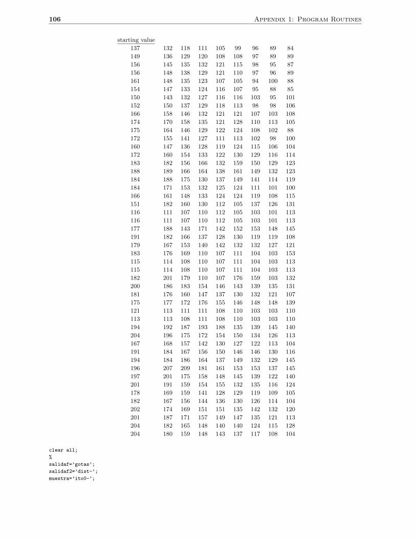
106 Appendix 1: Program Routines
starting value
137 132 118 111 105 99 96 89 84
149 136 129 120 108 108 97 89 89
156 145 135 132 121 115 98 95 87
156 148 138 129 121 110 97 96 89
161 148 135 123 107 105 94 100 88
154 147 133 124 116 107 95 88 85
150 143 132 127 116 116 103 95 101
152 150 137 129 118 113 98 98 106
166 158 146 132 121 121 107 103 108
174 170 158 135 121 128 110 113 105
175 164 146 129 122 124 108 102 88
172 155 141 127 111 113 102 98 100
160 147 136 128 119 124 115 106 104
172 160 154 133 122 130 129 116 114
183 182 156 166 132 159 150 129 123
188 189 166 164 138 161 149 132 123
184 188 175 130 137 149 141 114 119
184 171 153 132 125 124 111 101 100
166 161 148 133 124 124 119 108 115
151 182 160 130 112 105 137 126 131
116 111 107 110 112 105 103 101 113
116 111 107 110 112 105 103 101 113
177 188 143 171 142 152 153 148 145
191 182 166 137 128 130 119 119 108
179 167 153 140 142 132 132 127 121
183 176 169 110 107 111 104 103 153
115 114 108 110 107 111 104 103 113
115 114 108 110 107 111 104 103 113
182 201 179 110 107 176 159 103 132
200 186 183 154 146 143 139 135 131
181 176 160 147 137 130 132 121 107
175 177 172 176 155 146 148 148 139
121 113 111 111 108 110 103 103 110
113 113 108 111 108 110 103 103 110
194 192 187 193 188 135 139 145 140
204 196 175 172 154 150 134 126 113
167 168 157 142 130 127 122 113 104
191 184 167 156 150 146 146 130 116
194 184 186 164 137 149 132 129 145
196 207 209 181 161 153 153 137 145
197 201 175 158 148 145 139 122 140
201 191 159 154 155 132 135 116 124
178 169 159 141 128 129 119 109 105
182 167 156 144 136 130 126 114 104
202 174 169 151 151 135 142 132 120
201 187 171 157 149 147 135 121 113
204 182 165 148 140 140 124 115 128
204 180 159 148 143 137 117 108 104
clear all;
%
salidaf=’gotas’;
salidaf2=’dist-’;
muestra=’ito0-’;

Section A.1 107
formato=’.jpg’;
tipf=’.dat’;
nombre2=strcat(salidaf,tipf);
uuu=fopen(nombre2,’w+’);
%
% Datos inicales de centros X y Y.
%
format long e
frecuencia=5;
deltas=load(’ito-delta.dat’);
CentrosX=load(’ito-centrosx.dat’);
CentrosY=load(’ito-centrosy.dat’);
Radios=load(’ito-RADIO.dat’);
recortes=load(’recortes’); % revisar fecha de experimento
umbral=load(’tresholds’); %archivo con los valores de bin, tiempo y treshold.
[au bu]=size(umbral);
%l=0;
%for i=0:15:105
%l=l+1;
%if(i == 0)
%i=12;
%end
%tiempos(l)=i;
%end
tiempos=[4 10 30 60 120 150 240 330 450]’;
l=0;
for i=0:250:2000
l=l+1;
if(i==0)
i=1;
end
if(i==2000)
i=2048;
end
h(l)=i;
end
l=0;
for i=0:250:1500
l=l+1;
if(i==0)
i=1;
end
if(i==1500)
i=1536;
end
v(l)=i;
end
recx=recortes(1,4);
recy=recortes(1,5);
factor=1.390625*500/322.58;
nft=1;
inicio=4;
%numfoto=max(size(Radios));
numfoto=450;
%
% Inicia ciclo.
%
l=1;
for nft=inicio:numfoto
nfoto=num2str(nft);
nombre=strcat(muestra,nfoto,formato);
I=imread(nombre);
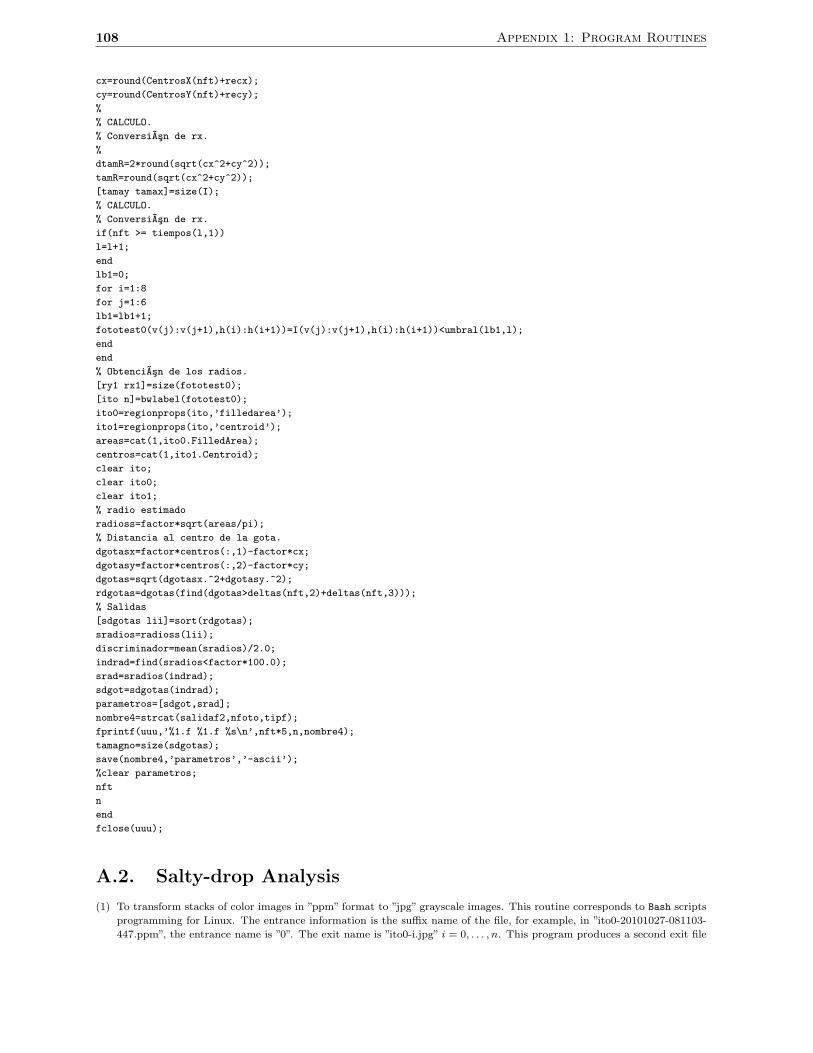
108 Appendix 1: Program Routines
cx=round(CentrosX(nft)+recx);
cy=round(CentrosY(nft)+recy);
%
% CALCULO.
% Conversi~Asn de rx.
%
dtamR=2*round(sqrt(cx^2+cy^2));
tamR=round(sqrt(cx^2+cy^2));
[tamay tamax]=size(I);
% CALCULO.
% Conversi~Asn de rx.
if(nft >= tiempos(l,1))
l=l+1;
end
lb1=0;
for i=1:8
for j=1:6
lb1=lb1+1;
fototest0(v(j):v(j+1),h(i):h(i+1))=I(v(j):v(j+1),h(i):h(i+1))<umbral(lb1,l);
end
end
% Obtenci~Asn de los radios.
[ry1 rx1]=size(fototest0);
[ito n]=bwlabel(fototest0);
ito0=regionprops(ito,’filledarea’);
ito1=regionprops(ito,’centroid’);
areas=cat(1,ito0.FilledArea);
centros=cat(1,ito1.Centroid);
clear ito;
clear ito0;
clear ito1;
% radio estimado
radioss=factor*sqrt(areas/pi);
% Distancia al centro de la gota.
dgotasx=factor*centros(:,1)-factor*cx;
dgotasy=factor*centros(:,2)-factor*cy;
dgotas=sqrt(dgotasx.^2+dgotasy.^2);
rdgotas=dgotas(find(dgotas>deltas(nft,2)+deltas(nft,3)));
% Salidas
[sdgotas lii]=sort(rdgotas);
sradios=radioss(lii);
discriminador=mean(sradios)/2.0;
indrad=find(sradios<factor*100.0);
srad=sradios(indrad);
sdgot=sdgotas(indrad);
parametros=[sdgot,srad];
nombre4=strcat(salidaf2,nfoto,tipf);
fprintf(uuu,’%1.f %1.f %s\n’,nft*5,n,nombre4);
tamagno=size(sdgotas);
save(nombre4,’parametros’,’-ascii’);
%clear parametros;
nft
n
end
fclose(uuu);
A.2. Salty-drop Analysis
(1) To transform stacks of color images in ”ppm” format to ”jpg” grayscale images. This routine corresponds to Bash scripts
programming for Linux. The entrance information is the suffix name of the file, for example, in ”ito0-20101027-081103-
447.ppm”, the entrance name is ”0”. The exit name is ”ito0-i.jpg” i = 0, . . . , n. This program produces a second exit file
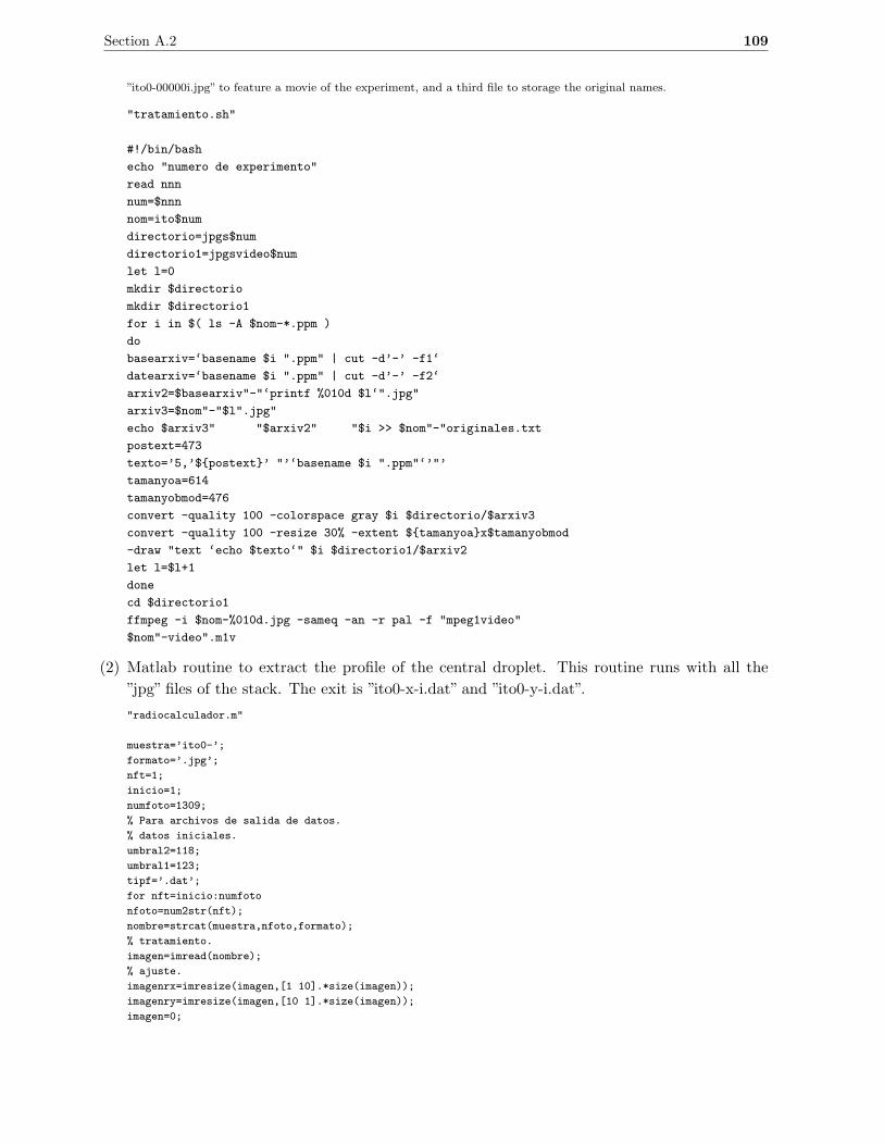
Section A.2 109
”ito0-00000i.jpg” to feature a movie of the experiment, and a third file to storage the original names.
"tratamiento.sh"
#!/bin/bash
echo "numero de experimento"
read nnn
num=$nnn
nom=ito$num
directorio=jpgs$num
directorio1=jpgsvideo$num
let l=0
mkdir $directorio
mkdir $directorio1
for i in $( ls -A $nom-*.ppm )
do
basearxiv=‘basename $i ".ppm" | cut -d’-’ -f1‘
datearxiv=‘basename $i ".ppm" | cut -d’-’ -f2‘
arxiv2=$basearxiv"-"‘printf %010d $l‘".jpg"
arxiv3=$nom"-"$l".jpg"
echo $arxiv3" "$arxiv2" "$i >> $nom"-"originales.txt
postext=473
texto=’5,’$postext’ "’‘basename $i ".ppm"‘’"’
tamanyoa=614
tamanyobmod=476
convert -quality 100 -colorspace gray $i $directorio/$arxiv3
convert -quality 100 -resize 30% -extent $tamanyoax$tamanyobmod
-draw "text ‘echo $texto‘" $i $directorio1/$arxiv2
let l=$l+1
done
cd $directorio1
ffmpeg -i $nom-%010d.jpg -sameq -an -r pal -f "mpeg1video"
$nom"-video".m1v
(2) Matlab routine to extract the profile of the central droplet. This routine runs with all the
”jpg” files of the stack. The exit is ”ito0-x-i.dat” and ”ito0-y-i.dat”.
"radiocalculador.m"
muestra=’ito0-’;
formato=’.jpg’;
nft=1;
inicio=1;
numfoto=1309;
% Para archivos de salida de datos.
% datos iniciales.
umbral2=118;
umbral1=123;
tipf=’.dat’;
for nft=inicio:numfoto
nfoto=num2str(nft);
nombre=strcat(muestra,nfoto,formato);
% tratamiento.
imagen=imread(nombre);
% ajuste.
imagenrx=imresize(imagen,[1 10].*size(imagen));
imagenry=imresize(imagen,[10 1].*size(imagen));
imagen=0;
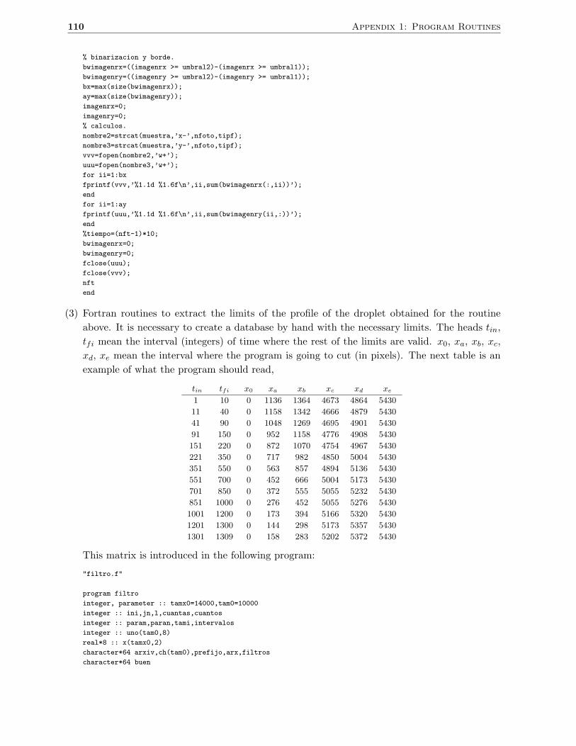
110 Appendix 1: Program Routines
% binarizacion y borde.
bwimagenrx=((imagenrx >= umbral2)-(imagenrx >= umbral1));
bwimagenry=((imagenry >= umbral2)-(imagenry >= umbral1));
bx=max(size(bwimagenrx));
ay=max(size(bwimagenry));
imagenrx=0;
imagenry=0;
% calculos.
nombre2=strcat(muestra,’x-’,nfoto,tipf);
nombre3=strcat(muestra,’y-’,nfoto,tipf);
vvv=fopen(nombre2,’w+’);
uuu=fopen(nombre3,’w+’);
for ii=1:bx
fprintf(vvv,’%1.1d %1.6f\n’,ii,sum(bwimagenrx(:,ii))’);
end
for ii=1:ay
fprintf(uuu,’%1.1d %1.6f\n’,ii,sum(bwimagenry(ii,:))’);
end
%tiempo=(nft-1)*10;
bwimagenrx=0;
bwimagenry=0;
fclose(uuu);
fclose(vvv);
nft
end
(3) Fortran routines to extract the limits of the profile of the droplet obtained for the routine
above. It is necessary to create a database by hand with the necessary limits. The heads tin,
tfi mean the interval (integers) of time where the rest of the limits are valid. x0, xa, xb, xc,
xd, xe mean the interval where the program is going to cut (in pixels). The next table is an
example of what the program should read,
tin tfi x0 xa xb xc xd xe
1 10 0 1136 1364 4673 4864 5430
11 40 0 1158 1342 4666 4879 5430
41 90 0 1048 1269 4695 4901 5430
91 150 0 952 1158 4776 4908 5430
151 220 0 872 1070 4754 4967 5430
221 350 0 717 982 4850 5004 5430
351 550 0 563 857 4894 5136 5430
551 700 0 452 666 5004 5173 5430
701 850 0 372 555 5055 5232 5430
851 1000 0 276 452 5055 5276 5430
1001 1200 0 173 394 5166 5320 5430
1201 1300 0 144 298 5173 5357 5430
1301 1309 0 158 283 5202 5372 5430
This matrix is introduced in the following program:
"filtro.f"
program filtro
integer, parameter :: tamx0=14000,tam0=10000
integer :: ini,jn,l,cuantas,cuantos
integer :: param,paran,tami,intervalos
integer :: uno(tam0,8)
real*8 :: x(tamx0,2)
character*64 arxiv,ch(tam0),prefijo,arx,filtros
character*64 buen
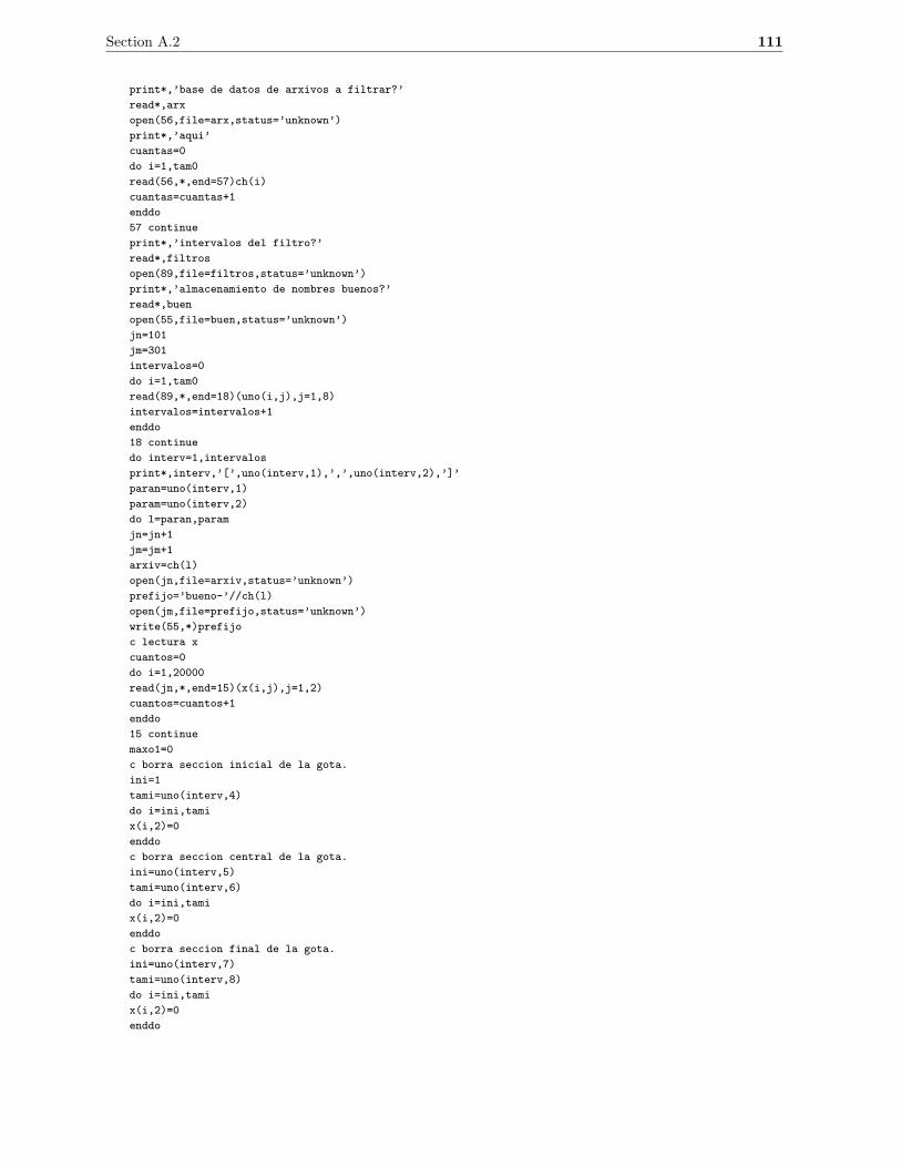
Section A.2 111
print*,’base de datos de arxivos a filtrar?’
read*,arx
open(56,file=arx,status=’unknown’)
print*,’aqui’
cuantas=0
do i=1,tam0
read(56,*,end=57)ch(i)
cuantas=cuantas+1
enddo
57 continue
print*,’intervalos del filtro?’
read*,filtros
open(89,file=filtros,status=’unknown’)
print*,’almacenamiento de nombres buenos?’
read*,buen
open(55,file=buen,status=’unknown’)
jn=101
jm=301
intervalos=0
do i=1,tam0
read(89,*,end=18)(uno(i,j),j=1,8)
intervalos=intervalos+1
enddo
18 continue
do interv=1,intervalos
print*,interv,’[’,uno(interv,1),’,’,uno(interv,2),’]’
paran=uno(interv,1)
param=uno(interv,2)
do l=paran,param
jn=jn+1
jm=jm+1
arxiv=ch(l)
open(jn,file=arxiv,status=’unknown’)
prefijo=’bueno-’//ch(l)
open(jm,file=prefijo,status=’unknown’)
write(55,*)prefijo
c lectura x
cuantos=0
do i=1,20000
read(jn,*,end=15)(x(i,j),j=1,2)
cuantos=cuantos+1
enddo
15 continue
maxo1=0
c borra seccion inicial de la gota.
ini=1
tami=uno(interv,4)
do i=ini,tami
x(i,2)=0
enddo
c borra seccion central de la gota.
ini=uno(interv,5)
tami=uno(interv,6)
do i=ini,tami
x(i,2)=0
enddo
c borra seccion final de la gota.
ini=uno(interv,7)
tami=uno(interv,8)
do i=ini,tami
x(i,2)=0
enddo
112 Appendix 1: Program Routines
c escribe el vector a analizar.
do i=1,cuantos
write(jm,*)(x(i,j),j=1,2)
enddo
close(jn)
close(jm)
enddo
enddo
close(100)
end
(4) Fortran routine to extract limits of the profile of the central drop in the horizontal orientation.
The entrance is a file with the list of files called ”ito0-x-i.dat”, this file can be obtained by the
execution of the Linux command,
ls ito0-x-?.dat > namex
the exit files will provide information of the radius of the central drop as a function of time,
the geometric center, and the extreme coordinates for the horizontal orientation.
"radiosx.f"
program radios
integer, parameter :: tamx0=14000
integer :: cent,k
real*8 :: x(tamx0,2),rx(tamx0,2),R(tamx0)
real*8 :: maxo0,maxo1
character*64 ch(tamx0),arxiv,arx
print*,’base de datos de arxivos a analizar?’
read*,arx
open(50,file=arx,status=’unknown’)
open(51,file=’ito-radiosx.dat’,status=’unknown’)
open(52,file=’ito-centrosx.dat’,status=’unknown’)
open(53,file=’ito-extremosx.dat’,status=’unknown’)
factor=1.390625*500/(3225.8*2)
k=0
do i=1,tamx0
read(50,*,end=18)ch(i)
k=k+1
enddo
18 continue
print*,k
print*,’centro probable de la gota (entero>0)?’
read*,cent
jn=101
do l=1,k
arxiv=ch(l)
open(jn,file=arxiv,status=’unknown’)
kk=0
do i=1,tamx0
read(jn,*,end=19)(x(i,j),j=1,2)
kk=kk+1
enddo
19 continue
c print*,l,kk
maxo0=0
do i=1,cent
maxo0=max(x(i,2),maxo0)
enddo
ll=0
Section A.2 113
do i=1,cent
if(x(i,2) .eq. maxo0) goto 20
ll=ll+1
enddo
20 continue
rx(l,1)=ll
maxo1=0
do i=cent,kk
maxo1=max(x(i,2),maxo1)
enddo
ll=cent
do i=cent,kk
if(x(i,2) .eq. maxo1) goto 21
ll=ll+1
enddo
21 continue
rx(l,2)=ll
R(l)=rx(l,2)-rx(l,1)
centrox=rx(l,2)-R(l)/2
write(51,*)l*5,R(l)*factor
write(52,*)centrox/10
write(53,*)rx(l,1)/10,rx(l,2)/10
close(jn)
enddo
close(50)
close(51)
close(52)
close(53)
end
(5) Fortran routine to extract limits of the profile of the central drop in the vertical orientation.
Similar than the last program, the entrance would be a matrix, and the exit will provide
geometric information of the central drop.
"radiosy.f"
program radios
integer, parameter :: tamx0=14000
integer :: cent,k
real*8 :: x(tamx0,2),rx(tamx0,2),R(tamx0)
real*8 :: maxo0,maxo1
character*64 ch(tamx0),arxiv,arx
print*,’base de datos de arxivos a analizar?’
read*,arx
open(50,file=arx,status=’unknown’)
open(51,file=’ito-radiosy.dat’,status=’unknown’)
open(52,file=’ito-centrosy.dat’,status=’unknown’)
open(53,file=’ito-extremosy.dat’,status=’unknown’)
factor=1.390625*500/(3225.8*2)
k=0
do i=1,tamx0
read(50,*,end=18)ch(i)
k=k+1
enddo
18 continue
print*,k
print*,’centro probable de la gota (entero>0)?’
read*,cent
jn=101
do l=1,k
arxiv=ch(l)
open(jn,file=arxiv,status=’unknown’)
114 Appendix 1: Program Routines
kk=0
do i=1,tamx0
read(jn,*,end=19)(x(i,j),j=1,2)
kk=kk+1
enddo
19 continue
c print*,l,kk
maxo0=0
do i=1,cent
maxo0=max(x(i,2),maxo0)
enddo
ll=0
do i=1,cent
if(x(i,2) .eq. maxo0) goto 20
ll=ll+1
enddo
20 continue
rx(l,1)=ll
maxo1=0
do i=cent,kk
maxo1=max(x(i,2),maxo1)
enddo
ll=cent
do i=cent,kk
if(x(i,2) .eq. maxo1) goto 21
ll=ll+1
enddo
21 continue
rx(l,2)=ll
R(l)=rx(l,2)-rx(l,1)
centrox=rx(l,2)-R(l)/2
write(51,*)l*5,R(l)*factor
write(52,*)centrox/10
write(53,*)rx(l,1)/10,rx(l,2)/10
close(jn)
enddo
close(50)
close(51)
close(52)
close(53)
end
(6) Fortran routine to obtain the mean radius. This routine needs the entrance of ”ito-radiosx.dat”,
”ito-radiosy.dat” and the possible center for both orientations.
"unidor.f"
program unidor
integer,parameter :: n=1000000
integer l
real*8 :: xr1(n,2),z(n),xr2(n,2)
open(100,file=’ito-radiosx.dat’,status=’old’)
open(101,file=’ito-radiosy.dat’,status=’old’)
open(102,file=’ito-RADIO.dat’,status=’unknown’)
open(103,file=’ito-RADIOP.dat’,status=’unknown’)
l=0
do i=1,n
l=l+1
read(100,*,end=18)(xr1(i,j),j=1,2)
read(101,*,end=18)(xr2(i,j),j=1,2)
z(i)=(xr1(i,2)+xr2(i,2))/2.0
enddo
Section A.2 115
18 continue
print*,l
do i=1,l
write(102,*)xr1(i,1)/2.0,z(i)
enddo
do i=1,l,30
write(103,*)xr1(i,1)/2.0,z(i)
enddo
close(100)
close(101)
close(102)
close(103)
end
(7) With the information of the center drop radius and its center per each time, this Matlab
routine relocate the original image ”jpg” into a new image which its center is the geometric
center of the central drop. Also, this routine increases the frame of the original picture into a
square frame. Once these operation are done, the image is converted into polar coordinates;
the central drop becomes a rectangle, the depletion zone and the rest of the pattern too. Now,
the distance between the central drop and small droplets can be computed. This program
should be copied into the same folder of the image stack in ”jpg” format.
salidaf1=’dens-’;
tipf=’.dat’;
salidaf11=’R-dens-’;
tipf=’.dat’;
frecuencia=5;
%%% Datos inicales de centros X y Y.
CentrosX=load(’ito-centrosx.dat’);
CentrosY=load(’ito-centrosy.dat’);
umbral=load(’umbrales’);
recortes=load(’recortes’); % revisar fecha de experimento
umbraln=umbral(1,2); % revisar fecha de experimento
recx=recortes(1,4);
recy=recortes(1,5);
factor=1.390625*500/322.58;
muestra=’ito0-’;
formato=’.jpg’;
nft=1;
inicio=1;
numfoto=20;
%numfoto=1309;
%numfoto=size(CentrosX);
%numfoto=size(CentrosX)(1); %octave
%intervalo=10
for nft=inicio:numfoto
%for nft=inicio:intervalo:numfoto
nfoto=num2str(nft);
nombre=strcat(muestra,nfoto,formato);
%I=jpgread(nombre);
I=imread(nombre);
cx=round(CentrosX(nft)+recx);
cy=round(CentrosY(nft)+recy);
% CALCULO %%%%%%%%%%%%%%%%%%%%%%%%%%%%%%%%%
% conversi~Asn de rx.
tiempo=(nft)*10;
dtamR=2*round(sqrt(cx^2+cy^2));
tamR=round(sqrt(cx^2+cy^2));
[tamay tamax]=size(I);
Ax=round(tamR-cx);
116 Appendix 1: Program Routines
Ay=round(tamR-cy);
II=ones(dtamR,dtamR)*(-1);
II(Ay:tamay+Ay-1,Ax:tamax+Ax-1)=I;
clear I;
[iimax jjmax]=size(II);
xcc=round(iimax/2);
ycc=round(jjmax/2);
ima=2*ceil(iimax/2)-1;
imax=round(ima/sqrt(2));
jma=2*ceil(jjmax/2)-1;
jmax=round(jma/sqrt(2));
xc=(imax+1)/2;
yc=(jmax+1)/2;
xmac=(ima+1)/2;
ymac=(jma+1)/2;
foto1(1:ima,1:jma)=II(xcc-(ima-1)/2:xcc+(ima-1)/2,ycc-(jma-1)/2:ycc+(jma-1)/2);
angulo=2*pi;
rrrmax=0.5-eps;
N=round(rrrmax*max(jma,ima));
M=(round(angulo*rrrmax*max(jma,ima)));
desenrollada=zeros(N,M);
factorM=angulo/(M-1);
factorN=rrrmax/(N-1);
c2=1:M;
c1=1:N;
cc2=(c2-1)*factorM;
ccrad1=factorN*(c1-1);
coorccx=round(ima*ccrad1’*sin(cc2))+xmac;
coorccy=round(jma*ccrad1’*cos(cc2))+ymac;
coorccc=coorccx+ ima*(coorccy-1);
desenrollada=foto1(coorccc);
clear foto1;
[teta rx]=size(desenrollada);
dry=10; %delta en r en pixeles.
% ciclo de obtenci~Asn de
for j=1:teta-dry
foto=desenrollada(j:j+dry,:);
conta(j)=sum(sum(foto > -1));
conta1(j)=sum(sum(foto > -1 & foto < umbraln));
clear foto;
end
aspecto=(conta1./conta)’;
nombre3=strcat(salidaf1,nfoto,tipf);
uuu=fopen(nombre3,’w+’);
fprintf(uuu,’%1.4f\n’,aspecto);
fclose(uuu);
clear aspecto;
end
(8) The following Matlab routine computes the distance
muestra=’dens-’;
formato=’.dat’;
%%%%%%%%%%%%%% Frecuencia de adquisici~Asn de fotos.
frecuencia=5;
factor=500*1.390625/322.58; %conversi~Asn pixel Atm.
%%%%%%%%%%%%%%%%%%%%% Datos inicales de di~Aametros X, Y y centros.
Radios=load(’-ascii’,’ito-RADIO.dat’);
Rpixel=round(Radios(:,2)/factor);
nft=1;
inicio=4;
numfoto=size(Radios);
% clear Radios;

Section A.2 117
%%%%%%%%%%%%%%%%%%%%%%%% INICIA LECTURA DE FOTOS
uuu=fopen(’ito-delta.dat’,’w+’);
for nft=inicio:numfoto
nfoto=num2str(nft);
nombre=strcat(muestra,nfoto,formato);
densi=load(nombre);
famosadelta(nft)=sum(densi(Rpixel:1200) < 0.0047 )*factor;
fprintf(uuu,’%1.1f %1.4f %1.4f\n’,Radios(nft,1),Radios(nft,2),famosadelta(nft)’);
clear densi;
end

118 Appendix 1: Program Routines
Appendix B
Appendix 2: Characterization of the
Condensation Chamber
As a starting work of collaboration between the laboratory of colloids and complex physics
at the Science Faculty of University of Navarra and the laboratory of fluid mechanic and turbu-
lence of Science Faculty, National University of Mexico, measurements of the flux inside a new
condensation chamber made in Mexico. The main purpose of this collaboration is to investigate
from the point of view of hydrodynamics to study the flux of vapors in many situations, like the
problem of the flux inside small cavity with walls at different temperature, the flux of immiscible
and miscible vapors.
B.1. Characterization
The characterization of the chamber under normal conditions (Ti < 10 C at the surface at
flux ≈ 250 ml/min) of operation was done with complementary measurements with the hot-wire
anemometry technique in the relevant regions like the zone nearby the inlets, the center of the
chamber and the exits at 90 of each inlet. The hot-wire probe is made of tungsten, and it works
at temperature and resistance of operation of To = 250 C and Ro = 8.95 MΩ. The probe is
set perpendicular with respect the surface work of the chamber and centered. This has been
displaced in X and Y directions. Per position, the acquisition of the velocity values was made
for one minute, it has been displaced every 2 mm. It has been proceeded with air and without to
decrease the temperature of the copper plate. Also, it has been done as in a normal experiment of
BF: the WV produced by bubbling air at room temperature is streamed at certain flux, and the
copper plated is cooled down at ≈10 C and a flow of 885 ml/min (per inlet). The results of both
techniques will be correlated with the direct observation of the whole work area. A correlation of
the magnitude of the velocity and the amount of accumulated water at one coordinate point is
expected. The field velocity on the concentric region of 70 cm2 exhibits a non symmetric velocity
field (Fig. B.2 and Fig. B.3). Due to the aquarium air pump used to flow the vapors, the flow
variates in the experiment of air. The flow reported for this case is 1328 ml/min.
119
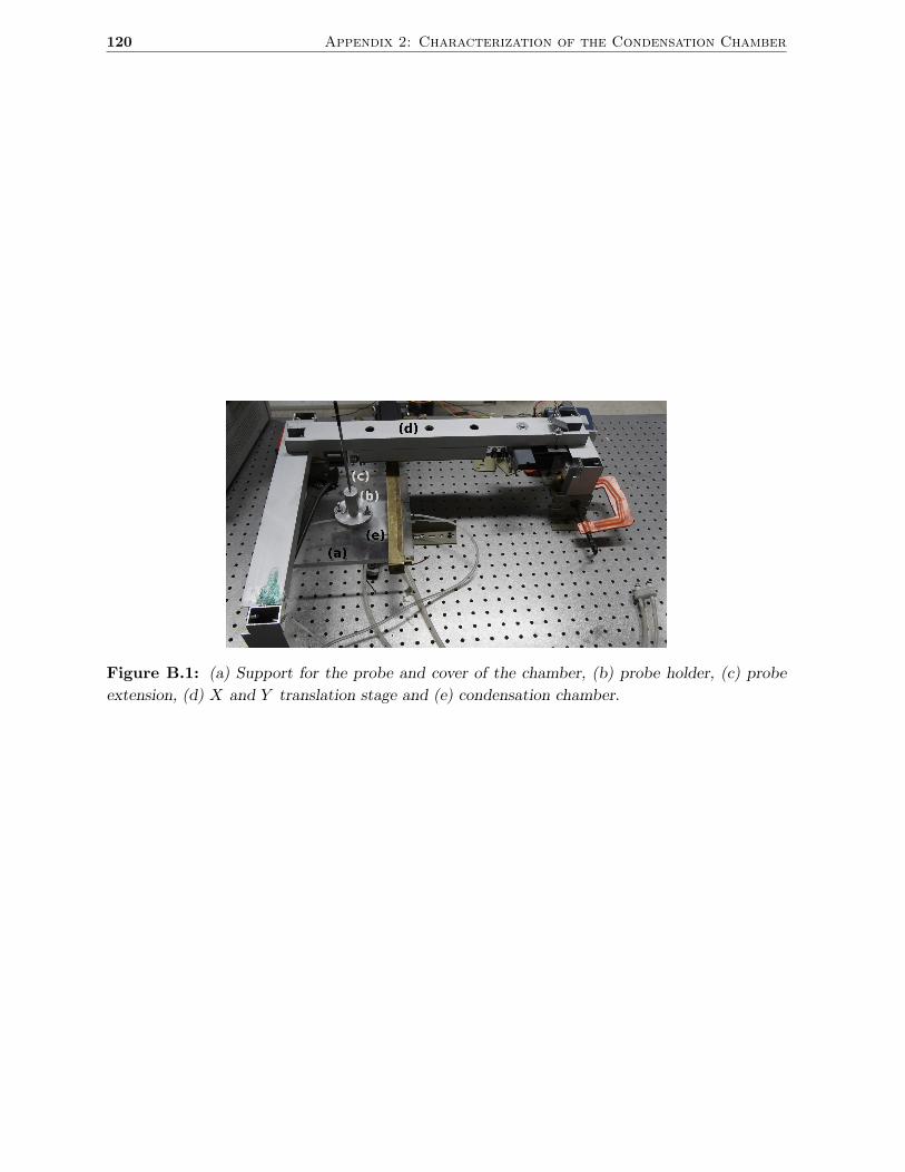
120 Appendix 2: Characterization of the Condensation Chamber
Figure B.1: (a) Support for the probe and cover of the chamber, (b) probe holder, (c) probe
extension, (d) X and Y translation stage and (e) condensation chamber.
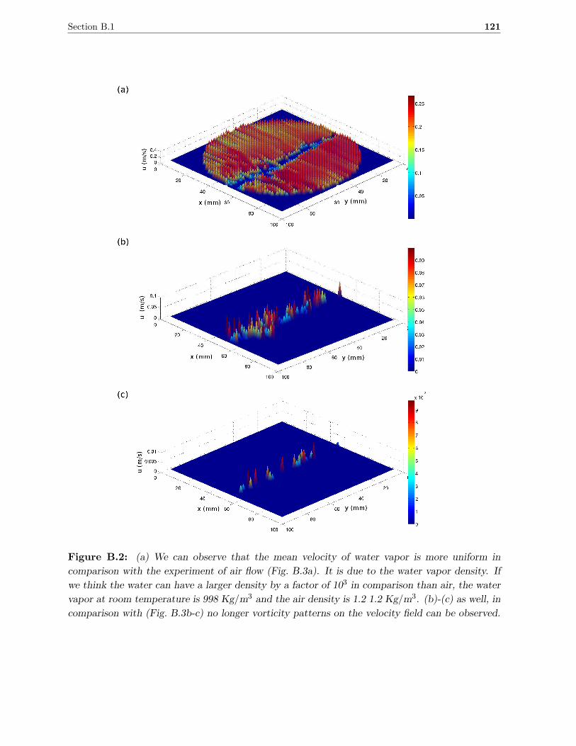
Section B.1 121
Figure B.2: (a) We can observe that the mean velocity of water vapor is more uniform in
comparison with the experiment of air flow (Fig. B.3a). It is due to the water vapor density. If
we think the water can have a larger density by a factor of 103 in comparison than air, the water
vapor at room temperature is 998 Kg/m3 and the air density is 1.2 1.2 Kg/m3. (b)-(c) as well, in
comparison with (Fig. B.3b-c) no longer vorticity patterns on the velocity field can be observed.
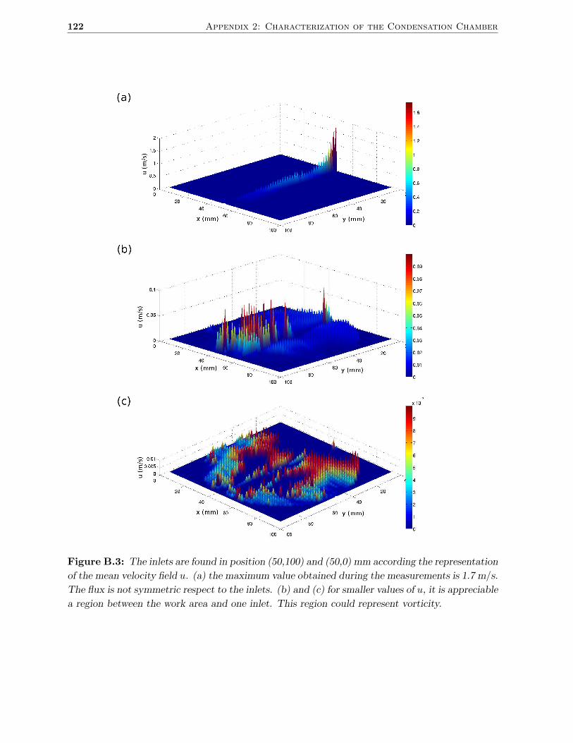
122 Appendix 2: Characterization of the Condensation Chamber
Figure B.3: The inlets are found in position (50,100) and (50,0) mm according the representation
of the mean velocity field u. (a) the maximum value obtained during the measurements is 1.7 m/s.
The flux is not symmetric respect to the inlets. (b) and (c) for smaller values of u, it is appreciable
a region between the work area and one inlet. This region could represent vorticity.
Appendix C
Appendix 3: HVAC Diagram
123
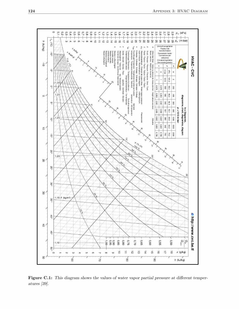
124 Appendix 3: HVAC Diagram
Figure C.1: This diagram shows the values of water vapor partial pressure at different temper-
atures [39].
Bibliography
[1] J. Guadarrama-Cetina, R. Narhe, W. Gonzalez-Vinas, D. Beysens. Droplet pattern and
condensation gradient around a humidity sink. Submitted .
[2] J. Guadarrama-Cetina, A. Mongruel, W. Gonzalez-Vinas, D. Beysens. Percolation-induced
frost formation. EPL (Europhysics Letters) 101 (1), (2013), p. 16009.
[3] J. Guadarrama-Cetina, W. Gonzalez-Vinas. Breath figures of two immiscible substances on
a repellent surface. Submitted .
[4] J. Aitken. Breath figures. Proceedings of the Royal Society of Edinburgh 20, (1893), pp.
94–97.
[5] J. Aitken. On some nuclei of cloudy condensation. Roy. Soc. Edin. 39, (1898), pp. 15–25.
[6] J. W. Giltay. Breath figures. Nature (86), (1911), pp. 585–585.
[7] J. Aitken. Breath figures. Nature (90), (1913), pp. 619–621.
[8] J. W. Rose, L. R. Glicksman. Dropwise condensation the distribution of drop sizes. Int. J.
Heat Mass Transfer 16, (1973), pp. 411–425.
[9] D. Beysens. Nucleation/nucleation. C. R. Physique 12, (2006), pp. 1082–1100.
[10] D. Beysens, C. M. Knobler. Growth of breath figures. Phys. Rev. Lett. 57 (12), (1986), pp.
1433–1436.
[11] F. Family, P. Meakin. Kinetics of droplet growth processes: Simulations, theory, and experi-
ments. Phys. Rev. A 40 (7), (1989), pp. 3836–3854.
[12] D. Fritter, D. Beysens. Experiment and simulation of the growth droplets on a surface (breath
figures). Phys. Rev. A. 43 (6), (1991), pp. 2858–2869.
[13] J. L. Katz. Homogeneous nucleation theory and experiment: A survey. Pure & Appl. Chern.
64 (11), (1992), pp. 1661–1666.
[14] A. Saito, Y. Utaka, S. Okawa, K. Matsuzawa, A. Tamaki. Fundamental research on the
supercooling phenomenon on heat transfer surfaces-investigation of an effect of characteristics
of surface and cooling rate on a freezing temperature of supercooled water. Int. J. Heat Mass
Transfer 33 (8), (1990), pp. 1607–1709.
[15] T. Hozumi, A. Saito, S. Okawa, T. Matsumura. Effect of bubble nuclei on freezing of super-
cooled water. Int. J. of Refrigeration 25, (2002), pp. 243–249.
125
126 BIBLIOGRAPHY
[16] A. W. Hodgson. Homogeneous nucleation. Advances in Colloid and Interface Science 21,
(1984), pp. 303–327.
[17] J. F. Lutsko. Communication: A dynamical theory of homogeneous nucleation for colloids
and macromolecules. J. Chem. Phys. 135, (2011), pp. 1–4.
[18] D. H. Rasmussen. Energetics of homogeneous nucleation - approach to a physical spinodal.
J. of Crystal Growth 56, (1981), pp. 45–55.
[19] A. V. Korolev. Rates of phase transformations in mixed-phase clouds. Q. J. R. Meteorol.
Soc. 134, (2008), pp. 595–608.
[20] K. Varanasi, T. Deng. Spatial control in the heterogeneous nucleation of water. App. Phys.
Lett. 094101 (95), (2009), pp. 1–3.
[21] K. Varanasi, N. Bhate. Frost formation and ice adhesion on superhydrophobic surfaces. App.
Phys. Lett. 234102 (97), (2010), pp. 1–3.
[22] A. Stayer, D. Beysens. Growth of droplets on a substrate by diffusion and coalescence. Phys.
Rev. A. 44 (12), (1991), pp. 8271–8277.
[23] J. D. Ford, A. Lekic. Rate of growth of drops during condensation. Int. J. Heat Mass Transfer
16, (1973), pp. 61–64.
[24] M. Sokuler, H.-J. Butt. Dynamics of condensation and evaporation: Effect of inter-drop
spacing. EPL 89, (1973), pp. 1–6.
[25] D. Beysens. The formation of dew. Atmospheric Research 39, (1995), pp. 215–237.
[26] T. M. Rogers, C. Desai. Droplet growth and coarsening during heterogeneous vapor conden-
sation. Phys. Rev. A 38 (10), (1988), pp. 5303–5309.
[27] P. L. Krapivsky. Growth of a single drop formed by diffusion and adsorption of monomers
on a two-dimensional substrates. Phys. Rev. E 47 (2), (1993), pp. 5303–5309.
[28] J. W. Rose. Condensation heat transfer fundamentals. Trans. IChem. E 76, (1998), pp.
143–152.
[29] R. D. Narhe, D. A. Beysens, Y. Pomeau. Dynamic drying in the early-stage coalescence of
droplets sitting on a plate. EPL 81, (2008), pp. 1–6.
[30] P. Meakin. Droplet deposition growth and coalescence. Rep. Prog. Phys. 55 (2), (1992), pp.
169–169.
[31] F. Family, P. Meakin. Scaling in the kinetics of droplet growth and coalescence: heterogeneous
nucleation. J. Phys. A: Math. Gen. 22, (1989), pp. 225–230.
[32] R. D. Narhe, K. P. A. M. D. Khandkar, A. V. Limaye, S. R. Sainkar, S. B. Ogale. Difference
in the dynamic scaling behavior of droplet size distribution for coalescence under pulsed and
continuous vapor delivery. Phys. Rev. Lett. 86 (8), (2001), pp. 1–9.
BIBLIOGRAPHY 127
[33] B. J. Briscoe, K. P. Galvin. The evolution of a 2d constrained growth system of droplets-breath
figures. J. Phys. D: Appl. Phys. 23, (1989), pp. 422–428.
[34] B. J. Briscoe, K. P. Galvin. Rapid communication: breath figures. J. Phys. D: Appl. Phys.
23, (1990), pp. 1265–1266.
[35] B. J. Briscoe, K. P. Galvin. Growth with coalescence during condensation. Phys. Rev. A
43 (4), (1990), pp. 422–428.
[36] M. Bachman. RCA-1 Silicon Wafer Cleaning (1999). Engeenering the Microworld at The
University of California, Irvine.
[37] W. Kern, E. J. Vossen. Thin film processes (1978).
[38] B. Elmar. Microdrops Evaporating on AFM Cantilevers, vol. 134 of Progress in Colloid and
Polymer Science. Springer Berlin / Heidelberg (2008). 10.1007/2882 2008 084.
[39] Unfortunatelly this information is not available. HVAC-CVC, http://www.cvc.be.tf.
[40] D. R. Lide. CRC Handbook of Chemistry and Physics. Taylor and Francis Group LLC, 87
edn. (2007).
[41] A. Quarteroni, F. Saleri. Scientific computing with matlab and Octave. Texts in computing
science and engineering. Springer, 2 edn. (2006).
[42] T. M. Inc. Matlab, the languaje of technical computing (1997).
[43] J. S. Owens. Condensation of water from the air upon hygroscopic crystals. Roy. Soc. Proc.
101, (1922), pp. 738–752.
[44] R. Williams, J. Blanc. Inhibition of water condensation by a soluble salt nucleus. J. Chem.
Phys. 74 (8), (1981), pp. 4675–4677.
[45] C. Schafle, P. Leiderer, C. Bechinger. Subpattern formation during condensation processes
on structured substrates. Europhysics Lett. 63 (3), (2003), pp. 394–400.
[46] D. E. Hare, C. M. Sorensen. The density of supercooled water. ii. bulk samples cooled to the
homogeneous nucleation limit. J. Chem. Phys. 87, (1987), pp. 40–45.
[47] A. Angell. Highs and lows in the density of water. Nature Nanotechnology 2, (2007), pp.
396–398.
[48] A. Saito, Y. Utaka, S. Okawa, K. Matsuzawa, A. Tamaki. Fundamental research on the
supercooling phenomenon on heat transfer surfaces investigation of an effect of characteristics
of surface and cooling rate on a freezing temperature of supercooled water. Int. J. Heat Mass
Trans. 33 (8), (1989), pp. 1697–1709.
[49] J. Castaing-Lasvignottes, T. David, J.-P. Bedecarrats, F. Strub. Dynamics modeling and ex-
perimental study of an ice generator heat exchanger using supercooled water. Eng. Conversion
and Management 47, (2006), pp. 3644–3651.
128 BIBLIOGRAPHY
[50] B. Na, R. L. Webb. A fundamental understanding of factors affecting first nucleation. Int.
J. Heat Mass Transfer 46, (2003), pp. 3797–3808.
[51] J. Qvist, H. Schober, B. Halle. Structural dynamics of supercooled water from quasielastic
neutron scattering and molecular simulations. J. Chem. Phys. 134, (2011), pp. 1–9.
[52] D. M. Murphy, T. Koop. Review of the vapour pressures of ice and supercooled water for
atmospheric applications. Q. J. R. Meteorol. Soc. 131, (2005), pp. 1539–1565.
[53] K. G. Libbrecht. Morphogenesis on ice: The physics of snow crystals. Eng. and Sc. (1),
(2001), pp. 10–19.
[54] J. Ji, Y. Zhao, L. Guo, B. Liu, C. Jib, P. Yang. Interfacial organic synthesis in a simple
droplet-based microfluidic system. Lab on a Chip, The Royal Society of Chemistry 12, (2012),
pp. 1373–1377.
[55] R. G. Sardesai, D. R. Webb. Condensation of binary vapours of immiscible liquids. Chemical
Eng. Science 34 (4), (1982), pp. 529–537.
[56] O. Tutkun. Condensation of vapours of binary immiscible liquids. Chem. Eng. and Processing
32, (1993), pp. 263–212.
[57] V. D. Rao, V. M. Krishna, K. Sharma, P. M. Rao. Convective condensation of vapor in the
presence of a non-condensable gas of high concentration in laminar flow in a vertical pipe.
Int. J. of Heat. and Mass Transfer 51, (2008), pp. 6090–6101.
[58] P. Borckmans, G. Dewel, A. de Wit, E. Dulos, J. Boissonade, F. Gauffre, P. de Kepper.
Diffusive instabilities and chemical reactions. Int. J. of Bifurcation and Chaos 12 (11),
(2002), pp. 2307–2332.
[59] U. Heiko, F. Bunz. Breath figures as a dynamic templating method for polymers and nano-
materials. Adv. Mater. 18, (2006), pp. 973–989.
[60] R. Kofman, M. Allione, F. Celestini, Z. Barkay, Y. Lereah. Preparation and analysis of a
two-components breath figure at the nanoscale. Eur. Phys. J. D 50, (2008), pp. 279–284.
[61] J. Rayleigh. Breath figures. Nature 2174 (86), (1911), p. 416.
[62] T. J. Baker. Breath figures. Philos. Mag. 44, (1922), p. 752.
[63] B. Lewis, J. Anderson. Nucleation and Growth of Thin Films. Academic London, 87 edn.
(1978).
[64] A. Steyer, P. Guenoun, D. Beysens. Spontaneous jumps of droplet. Phys. Rev. Lett 68 (1),
(1992), pp. 64–66.
[65] B. J. Briscoe, K. P. Galvin. The evolution of a 2d constrained growth system of droplets-breath
figures. J. Phys. D: Appl. Phys. 23 (68), (1990), pp. 422–428.
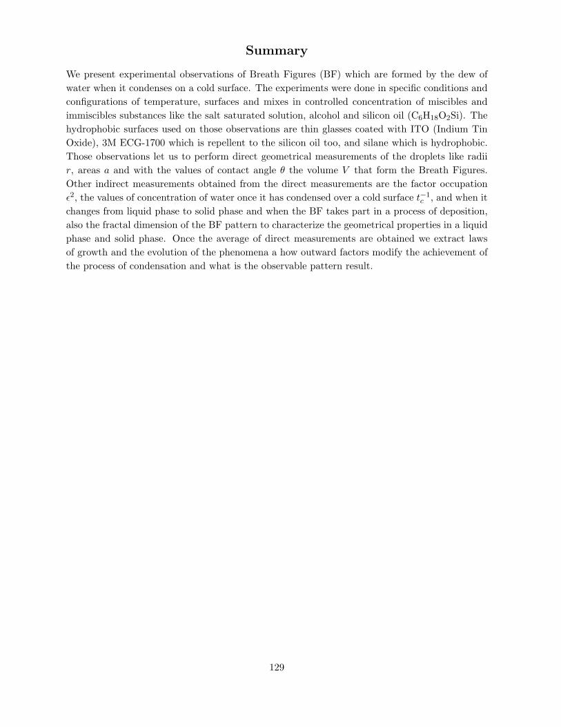
Summary
We present experimental observations of Breath Figures (BF) which are formed by the dew of
water when it condenses on a cold surface. The experiments were done in specific conditions and
configurations of temperature, surfaces and mixes in controlled concentration of miscibles and
immiscibles substances like the salt saturated solution, alcohol and silicon oil (C6H18O2Si). The
hydrophobic surfaces used on those observations are thin glasses coated with ITO (Indium Tin
Oxide), 3M ECG-1700 which is repellent to the silicon oil too, and silane which is hydrophobic.
Those observations let us to perform direct geometrical measurements of the droplets like radii
r, areas a and with the values of contact angle θ the volume V that form the Breath Figures.
Other indirect measurements obtained from the direct measurements are the factor occupation
ǫ2, the values of concentration of water once it has condensed over a cold surface t−1c , and when it
changes from liquid phase to solid phase and when the BF takes part in a process of deposition,
also the fractal dimension of the BF pattern to characterize the geometrical properties in a liquid
phase and solid phase. Once the average of direct measurements are obtained we extract laws
of growth and the evolution of the phenomena a how outward factors modify the achievement of
the process of condensation and what is the observable pattern result.
129
Resumen
Presentamos observaciones experimentales del fenomeno figuras de aliento (o BF por Breath
Figure) el cual se forma por el rocıo de agua cuando esta condensa en una superficie frıa. Se
han hecho experimentos con condiciones y configuraciones especıficas de temperatura, superficies
y concentraciones de mezclas de sustancias miscibles e inmiscibles como una solucion saturada
de sal, alcohol y hexametildisiloxano (C6H18O2Si). Las superficies hidrofobicas utilizadas en las
observaciones son vidrios recubiertos con oxido titanio e indio, 3M ECG-1700 el cual es repelente
al hexametildisiloxano tambien, ası como el silano tambien tiene propiedades hidrofobicas. Estas
observaciones nos permiten llevar acabo mediciones directas de la geometrıa de gotas, como el
radio r y el area a, angulos de contacto θ y volumenes V que forman los Breath Figures. Otras
medidas indirectas son obtenidas de mediciones directas son el factor de ocupacion ǫ2, los valores
de concentracion de agua una vez ha condensado sobre la superficie t−1c , y cuando esta cambia de
fase lıquida a solida y cuando el BF toma parte en el proceso de deposicion, tambien la dimension
fractal de los patrones del BF que caracterizan sus propiedades geometricas en la fase lıquida
o solida. Una vez que se ha obtenido el promedio de mediciones directas se esxtraen leyes de
crecimiento y la evolucion de los fenomenos y como factores externos modifican el desempeno del
proceso y las observables del patron resultante.
130


