Embed Size (px)
Citation preview

arX
iv:0
710.
0196
v3 [
hep-
ph]
10
Apr
200
8
Faddeev calculation of pentaquark Θ+
in the Nambu-Jona-Lasinio model-baseddiquark picture
H. Mineo a,b,c,1, J.A. Tjon a,d, K. Tsushima e,f,g,2 and Shin Nan Yang a
a Department of Physics, National Taiwan University, Taipei 10617, Taiwanb Institute of Atomic and Molecular Sciences, Academia Sinica,
P.O.Box 23-166, Taipei 10617, Taiwanc Institute of Applied Mechanics, National Taiwan University,
Taipei 10617, Taiwand KVI, University of Groningen, The Netherlands
e National Center for Theoretical Sciences, Taipei, Taipei 10617, Taiwanf Grupo de Fısica Nuclear and IUFFyM, Universidad de Salamanca,
E-37008 Salamanca, Spaing Thomas Jefferson National Accelerator Facility, Theory Center,
Mail Stop 12H2, 12000 Jefferson Avenue, Newport News, VA 23606, USA
April 10, 2008
Abstract
A Bethe-Salpeter-Faddeev (BSF) calculation is performed for the pentaquark Θ+ inthe diquark picture of Jaffe and Wilczek in which Θ+ is a diquark-diquark-s three-bodysystem. Nambu-Jona-Lasinio (NJL) model is used to calculate the lowest order diagramsin the two-body scatterings of sD and DD. With the use of coupling constants determinedfrom the meson sector, we find that sD interaction is attractive in s-wave while DDinteraction is repulsive in p-wave. With only the lowest three-body channel considered,we do not find a bound 1
2
+pentaquark state. Instead, a bound pentaquark Θ+ with 1
2
−
is obtained with a unphysically strong vector mesonic coupling constants.
1E-mail address: [email protected] address: [email protected]
1

1 Introduction
The report of the observation of a very narrow peak in theK+n invariant mass distribution[1, 2] around 1540 MeV in 2003, a pentaquark predicted in a chiral soliton model [3],triggered considerable excitement in the hadronic physics community. It has been labeledas Θ+ and included by the PDG in 2004 [4] under exotic baryons and rated with threestars. Very intensive research efforts, both theoretically and experimentally, ensued.
On the experimental side, practically all studies conducted after the first sightings wereconfirmed by several other groups produced null results, casting doubt on the existenceof the five-quark state [5, 6]. Subsequently, PDG in 2006 reduced the rating from threeto one stars [4]. More recently, the ZEUS experiment at HERA [7] observed a signal forΘ+ in a high energy reaction, while H1 [7], SPHINX [8] and CLAS [9] did not see it. Thisdisagreement between the LEPS [1] and other experiments could possibly originate fromtheir differences of experimental setups and kinematical conditions. So the experimentalsituation is presently not completely settled [10, 11, 12].
Many theoretical approaches have been employed, in addition to the chiral solitonmodel [3], including quark models [13], QCD sum rules [15], and lattice QCD [16] to un-derstand the properties and structure of Θ+. Several interesting ideas were also proposedon the pentaquark production mechanism. Review of the theoretical activities in the lastcouple of years can be found in Refs. [17, 18].
One of the most intriguing theoretical ideas suggested for Θ+ is the diquark picture ofJaffe and Wilczek (JW) [19] in which Θ+ is considered as a three-body system consistedof two scalar, isoscalar, color 3 diquarks (D’s) and a strange antiquark (s). It is based,in part, on group theoretical consideration. It would hence be desirable to examine sucha scheme from a more dynamical perspective.
The idea of diquark is not new. It is a strongly correlated quark pair and has beenadvocated by a number of QCD theory groups since 60’s [20, 21, 22]. It is known thatdiquark arises naturally from an effective quark theory in the low energy region, theNambu-Jona-Lasinio (NJL) model [23, 24]. NJL model conveniently incorporates oneof the most important features of QCD, namely, chiral symmetry and its spontaneouslybreaking which dictates the hadronic physics at low energy. Models based on NJL type ofLagrangians have been very successful in describing the low energy meson physics [25, 26].Based on relativistic Faddeev equation the NJL model has also been applied to the baryonsystems [27, 28]. It has been shown that, using the quark-diquark approximation, onecan explain the nucleon static properties reasonably well [29, 30]. If one further take thestatic quark exchange kernel approximation, the Faddeev equation can be solved analyti-cally. The resulting forward parton distribution functions [31] successfully reproduce thequalitative features of the empirical valence quark distribution. The model has also beenused to study the generalized parton distributions of the nucleon [32]. Consequently, wewill employ NJL model to describe the dynamics of a diquark-diquark-antiquark system.To describe such a three-particle system, it is necessary to resort to Faddeev formalism.
Since the NJL model is a covariant-field theoretical model, it is important to userelativistic equations to describe both the three-particle and its two-particle subsystems.To this end, we will adopt Bethe-Salpeter-Faddeev (BSF) equation [33] in our study. Forpractical purposes, Blankenbecler-Sugar (BbS) [34] reduction scheme will be followed toreduce the four-dimensional integral equation into three-dimensional ones.
In Sec II, NJL model in flavor SU(3) will be introduced with focus on the diquark. TheNJL model is then used to investigate the antiquark-diquark and diquark-diquark interac-tion with Bethe-Salpeter equation in Sec. III. In Sec. IV, we introduce the Bethe-Salpeter-Faddeev equation and solve it for the system of strange antiquark-diquark-diquark withthe interaction obtained in Sec. III. Results and discussions are presented in Sec. V, and
2

we summarize in Sec. VI.
2 SU(3)f NJL model and the diquark
The flavor SU(3)f NJL Lagrangian takes the form
L = ψ(i6∂ −m)ψ + LI , (1)
where ψT = (u, d, s) is the SU(3) quark field, and m = diag(mu,md,ms) is the currentquark mass matrix. LI is a chirally symmetric four-fermi contact interaction. By a Fierztransformation, we can rewrite LI into a Fierz symmetric form LI,qq = 1
2(LI + F(LI)),where F stands for the Fierz rearrangement. It has the advantage that the direct andexchange terms give identical contribution.
In the qq channel, the chiral invariant LI,qq, is given by [35]
LI,qq = G1
[
(ψλafψ)2 − (ψγ5λa
fψ)2]
−G2
[
(ψγµλafψ)2 + (ψγµγ5λa
fψ)2]
− G3
[
(ψγµλ0fψ)2 + (ψγµγ5λ0
fψ)2]
−G4
[
(ψγµλ0fψ)2 − (ψγµγ5λ0
fψ)2]
+ · · · , (2)
where a = 0 ∼ 8, and λ0f =
√
23I. If we define G5 by −G5(ψiγ
µψj)2 = −(G2 + G3 +
G4)(ψiγµλ0
fψj)2 −G2(ψiγ
µλ8fψj)
2 where i, j = u, d, then G3, G4, G5 are related by G5 =
G2 + 23Gv , with Gv ≡ G3 +G4. In passing, we mention that the conventionally used Gω
and Gρ are related to G5, Gv by Gω = 2G5 and Gρ = 2G5 − 43Gv .
For the diquark channel we rewrite LI into an form (ψAψT )(ψTBψ), where A and Bare totally antisymmetric matrices in Dirac, isospin and color indices. We will restrictourselves to scalar, isoscalar diquark with color and flavor in 3 as considered in the JWmodel. The interaction Lagrangian for the scalar-isoscalar diquark channel [36, 37] isgiven by
LI,s = Gs
[
ψ(γ5C)λ2fβ
Ac ψ
T] [
ψT (C−1γ5)λ2fβ
Ac ψ]
, (3)
where βAc =
√
32λ
A(A = 2, 5, 7) corresponds to one of the color 3c states. C = iγ0γ2 is
the charge conjugation operator, and λ′s are the Gell-Mann matrices.The Bethe-Salpeter (BS) equation for the scalar diquark channel [36, 37] is given by
τs(q) = 4iGs − 2iGs
∫
d4k
(2π)4tr[(C−1γ5τ2
fβA))S(k + q)(γ5Cτ2
fβA)ST (−q)]τs(q), (4)
where the factors 4 and 2 arise from Wick contractions. S(k) = (6k −M + iǫ)−1 withM ≡ Mu = Md, the constituent quark mass of u and d quarks, generated by solving thegap equation. τs(q) is the reduced t-matrix which is related to the t-matrix by ts(q) =(γ5Cτ2
fβAc )τs(q)(C
−1γ5τ2fβ
Ac ). The solution to Eq. (4) is
τs(q) =4iGs
1 + 2GsΠs(q2), (5)
with
Πs(q2) = 6i
∫
d4k
(2π)4trD[γ5S(q)γ5S(k + q)]. (6)
The gap equation for u, d and s quarks are given by
Mi = mi − 8G1 < qiqi >, (7)
3

with
< qiqi >≡ −iNc
∫
d4k
(2π)4trD(S(k)), (8)
where i = u, d, s.The loop integrals in Eqs. (6) and (8) diverge and we need to regularize the four-
momentum integral by adopting some cutoff scheme. With regularization, we can solvethe gap equation and t-matrix of the diquark in Eqs. (5) and (8) to determine theconstituent quark and diquark masses. However, since our purpose in this work is not anexact quantitative analysis but rather a qualitatively study of the interactions inside Θ+,we will not adopt any regularization scheme and simply use the empirical values of theconstituent quark masses M = Mu,d = 400 MeV, Ms = 600 MeV, and the diquark massMD = 600 MeV as obtained in the study of the nucleon properties [27, 28, 29, 31, 32].
3 Two-body interactions for strange antiquark-
diquark (sD) and diquark-diquark (DD) channels
In the JW model for Θ+, the two scalar-isoscalar, color 3 diquarks must be in a color3 in order to combine with s into a color singlet. Since 3 is the antisymmetric part of3× 3 = 3⊕ 6, the diquark-diquark wave function must be antisymmetric with respect tothe rest of its labels. For two identical scalar-isoscalar diquarks [ud]0, only spatial labelsremain so that the spatial wave function must be antisymmetric under space exchange andthe lowest possible state is p-state. Since in JW’s scheme, Θ+ has the quantum numberof JP = 1
2
+, s would be in relative s-wave to the DD pair. Accordingly, we will consider
only the configurations where sD and DD are in relative s- and p-waves, respectively.We will employ Bethe-Salpeter-Faddeev equation [33] to describe such a three-particle
system of sDD. For consistency, we will use Bethe-Salpeter equation to describe two-particles subsystems like sD and DD, which reads as,
T = B +BG0T, (9)
where B is the sum of all two-body irreducible diagrams and G0 is the free two-bodypropagator. In momentum space, the resulting Bethe-Salpeter equation can be written as
T (k′, k;P ) = B(k′, k;P ) +
∫
d4k′′
B(k′, k′′
;P )G0(k′′
;P )T (k′′
, k;P ), (10)
where G0 is the free two-particle propagator in the intermediate states. k and P are,respectively, the relative and total momentum of the system.
In practical applications, B is commonly approximated by the lowest order diagramsprescribed by the model Lagrangian and will be denoted by V hereafter. In addition, itis often to further reduce the dimensionality of the integral equation (10) from four tothree, while preserving the relativistic two-particle unitarity cut in the physical region.It is well known (for example, Ref. [38]) that such a procedure is rather arbitrary andwe will adopt, in this work, the widely employed Blankenbecler-Sugar (BbS) reductionscheme [34] which, for the case of two spinless particles, amounts to replacing G0 in Eq.(10) by
G0(k, P ) =1
(P/2 + k)2 −m21
1
(P/2 − k)2 −m22
→ −i(2π)41
(2π)3
∫
ds′
s− s′ + iǫ
4

× δ(+)(
(P ′/2 + k)2 −m21
)
δ(+)(
(P ′/2 − k)2 −m22
)
= −2πiδ
(
k0 −E1(|~k|) − E2(|~k|)
2
)
GBbS(|~k|, s), (11)
with
GBbS(|~k|, s) =E1(|~k|) + E2(|~k|)2E1(|~k|)E2(|~k|)
1
s− (E1(|~k|) + E2(|~k|))2 + iǫ, (12)
where s = P 2 and P ′ =√
s′/sP . The superscript (+) associated with the delta func-tions mean that only the positive energy part is kept in the propagator, and E1,2(|~k|) ≡√
~k2 +m21,2.
3.1 sD potential and the t-matrix
In Fig. 1 we show the lowest order diagram, i.e., first order in LI,qq in sD scattering. Dueto the trace properties for Dirac matrices, only the scalar-isovector (ψλa
fψ)2, the vector-
isoscalar (ψγµλ0fψ)2, and the vector-isovector (ψγµλa
fψ)2 will contribute to the vertex
Γ. Furthermore, the isovector vertex (ψΓλafψ)2 will not contribute since the trace in
p p
k k+q
Γ=λ or λ f fa a γµ
(a=0,8)
g γ Cλ βA5
f
2 g C γ λ β
A5f2-1
s- s-
Di Df = pDi
+q
DD
p -kDi
psi-
psf-
Γ
Figure 1: sD potential of the lowest order in LI,qq.
flavor space vanishes,∑8
a=0(λaf )33trf (λ2
fλafλ
2f ) = 0. Thus only the vector-isoscalar term,
(ψγµλ0fψ)2, remains.
For the on-shell diquarks, the lower part of Fig. 1 which corresponds to the scalardiquark form factor, can be calculated as
(pDi + pDf )µFv(q2) = i
∫
d4k
(2π)4tr[(gDC
−1γ5λ2fβ
Ac )S(k + q)γµS(k)(gDγ
5Cλ2fβ
Ac )ST (k − pDi)]
= 6ig2D
∫
d4k
(2π)4tr[S(k + q)γµS(k)S(pDi − k)], (13)
where we have made use of the relations C−1(γµ)TC = −γµ, trc[βAc β
Ac ] = 3. gD is defined
by
g−2D = − ∂ΠD(p2)
∂p2
∣
∣
∣
∣
∣
p2=M2
D
, (14)
with
ΠD(p2) ≡ 6i
∫
d4k
(2π)4tr[S(k)S(p − k)], (15)
5

and MD is the diquark mass. Fv(0) is normalized as 2pµFv(0) = −g2D
∂ΠD(p2)∂pµ
, such that
Fv(0) = 1. 1
Then the matrix element of the potential VsD can be expressed as
< sfDf |V |siDi > = (−v(psi))(−iVsD)(pDi, pDf )v(psf )
= (+16i)(−Gv)(−v(psi))γµv(psf )[
(λ0f )33 · trf
(
λ0f (λ2
f )2)]
× (pDi + pDf )µFv(q
2)
trf ((λ2f )2)
, (16)
i.e.,
VsD =64
3GvFv(q
2)VsD(pDi, pDf ), (17)
withVsD(pDi, pDf ) = (6pDi + 6pDf )/2. (18)
Here the factor +16i in Eq. (16) arises from the Wick contractions, and the factortrf ((λ2
f )2) in Eq. (16) is introduced to divide Fv(q2), since the factor trf ((λ2
f )2) is already
included in the expression of Fv(q2) by a trace in flavor SU(3)f space.
=t sD +
pDi
= pDi+q
p- psf-
t sD
si
p's-
p'D
Figure 2: The BS equation for sD.
The three-dimensional scattering equation for the sD system is now given by
tsD(pDi, pDf ) = VsD(pDi, pDf )
+ 4π
∫
d|~p ′
D||~p ′
D|2(2π)3
1
2
∫ 1
−1dxiG
BbSsD (|~p ′
D|, s2)KsD(|~pDi|, |~p′
D|, xi)tsD(~p′
D, pDf ),
(19)
where xi ≡ pDi · p′
D, p ≡ ~p/|p|, s2 = (pDi + psi)2 = (pDf + psf )2, p0
Di =√
~p 2Di +M2
D,
p0Df =
√
~p 2Df +M2
D and
KsD(|~pDi|, |~p′
D|, xi) ≡ 64
3GvFv((p
′D − pDi)
2)KsD(pDi, p′D)|
p′D
0=√
~p′2
D+M2
D
,
KsD(pDi, p′D) = (6pDi + 6p ′
D)(−6p ′
s +Ms)/2,
with Ms being the constituent quark mass of s and s.
1In the actual calculation we use the dipole form factor, Fv(q2) ≡ (1 − q2/Λ2)−2 with Λ = 0.84 GeV sincethe q2 dependence for Fv(q2) in the NJL model is not well reproduced.
6

We also present the results for the interactions between diquark and u or d, whichwould be of interest when we study non-strange pentaquarks. One can just repeat thederivations we describe in the above and easily obtain
VuD = VdD = − 16G1Fs(q2) + 32G5Fv(q
2)VsD(pDi, pDf ), (20)
in analogous to Eqs. (17) and (18).We add in passing that, within tree approximation, the sign of the potential for sD is
opposite to that of VsD due to charge conjugation, i.e.,
VsD(pDf , pDi) = −VsD(pDi, pDf ). (21)
We can immediately write down the scattering equation for the sD as,
tsD(pDf , pDi) = VsD(pDf , pDi)
+ 4π
∫
d|~p ′
D||~p ′
D|2(2π)3
1
2
∫ 1
−1dxfG
BbSsD (|~p ′
D|, s2)KsD(|~pDf |, |~p′
D|, xf )tsD(~p′
D, pDi),
(22)
where xf ≡ pDf · p ′
D, GBbSsD (|~p ′
D|, s2) = GBbSsD (|~p ′
D|, s2), and
KsD(|~pDf |, |~p′
D|, xf ) ≡ 64
3GvFv((p
′D − pDf )2)KsD(pDf , p
′D)|
p′D
0=√
~p′2
D+M2
D
,
KsD(pDf , p′D) = −(6pDf + 6p ′
D)(6p ′
s +Ms)/2, (23)
with p′s = p′s.
3.2 Representation in ρ-spin notation
In the sD (or sD) center of mass system the wave function which describes the relativemotion in J = 1
2 , is given by the Dirac spinor of the following form (see [39, 40]),
ΨsD,ms(p0s, ~ps) =
(
φs1(p0s, |~ps|)
~σ · ps φs2(p0s, |~ps|)
)
χms , (24)
ΨsD,ms(p0s, ~ps) =
(
~σ · ps φs2(p0s, |~ps|)
φs1(p0s, |~ps|)
)
χms ,
= γ5
(
φs1(p0s, |~ps|)
~σ · ps φs2(p0s, |~ps|)
)
χms , (25)
ΨsD(p0s, ~ps) ≡ Ψ†
sD(p0s, ~ps)γ
0, (26)
ΨsD(p0s, ~ps) ≡ Ψ†
sD(p0s, ~ps)γ
0, (27)
where ~pD = −~ps = −~ps, i.e., ΨsD(p0s, ~ps) = ΨsD(p0
s,−~pD) and ΨsD(p0s, ~ps) = ΨsD(p0
s,−~pD).In the following we simply write p′Q = |~p ′
Q|, p′Qi(f) = |~p ′
Qi(f)| , Q = s, s or D. Note that
the index 1 (2) corresponds to large (small) components for both s and s quark spinors.For a discretization in spinor space, we define the complete set of ρ-spin notation
([39, 41]) for the operators OsD = VsD, tsD, VsD and KsD = KsD, KsD of sD:
OsD,nm(pDf , pDi) ≡ tr[Ω†n(psf )OsD(pDf , pDi)Ωm(psi)], (28)
KsD,nm(pDf , p′D, xf ) ≡ tr[Ω†
n(psf )KsD(pDf , p′D, xf )Ωm(p′s)], (29)
7

where n,m = 1, 2, Ω1(p) = Ω√2
and Ω2(p) = ~γ · p Ω√2, Ω = 1+γ0
2 . Ω1(p) and Ω2(p) satisfy
tr[Ω†n(p)Ωm(p′)] = δn1δm1 + p · p ′
δn2δm2.Concerning the sD spinor, the large and small components can be reversed by γ5,
with the minus sign which comes from the definitions Eqs. (25) and (27): ΨsDOΨsD =−ΨsDγ
5Oγ5ΨsD. Then we can define ρ-spin notation for sD i.e., OsD = VsD, tsD, VsD
and KsD = KsD, KsD,
OsD,nm(pDi, pDf ) ≡ −tr[Ω†n(psi)γ
5OsD(pDi, pDf )γ5Ωm(psf )], (30)
KsD,nm(pDi, p′D, xi) ≡ −tr[Ω†
n(psi)γ5KsD(pDi, p
′D, xi)γ
5Ωm(p′s)]. (31)
From Eqs. (19,22,28-31), each component n (n = 1, 2) of spinors for the sD satisfythe following quadratic equation:
φ†sn(psi)tsD,nm(pDi, pDf )φsm(psf ) = φ†sn(psi)[
VsD,nm(pDi, pDf )
+4π2∑
l=1
∫
dp′D(2π)3
p′2D
1
2
∫ 1
−1dxiG
BbSsD (p′D, s2)KsD,nl(pDi, p
′D, xi)tsD,lm(p′D, pDf )
]
φsm(psf ).
(32)
A similar equation can be obtained for the sD by exchanging i↔ f and s↔ s in Eq.(32).
The explicit expressions of the ρ-spin notation for Vs(s)D and Ks(s)D are given inappendix B. We note that there are important relations:
VsD,nm(p, q) = −VsD,nm(p, q),
VsD(p, q) = −VsD(p, q),
KsD,nm(|~p |, |~q |, xpq) = −KsD,nm(|~p |, |~q |, xpq),
KsD(|~p |, |~q |, xpq) = −KsD(|~p |, |~q |, xpq).
By the partial wave expansion in Eq. (69) in appendix A, the BS equation for tsD,nm
in Eq. (32) for s-wave can be written as
tlsD=0sD,nm(pDi, pDf ) = V lsD=0
sD,nm(pDi, pDf )+4π
∫
dp′
D
(2π)3p
′2D
2∑
l=1
GBbSsD (p
′
D, s2)KlsD=0sD,nl (pDi, p
′
D)tlsD=0sD,lm(p
′
D, pDf ).
(33)
3.3 DD potential and t-matrix
In the case ofDD interaction, the lowest order diagrams are depicted in Figs. 3(a) and (b),with (a) the quark rearrangement diagram and (b) of the first order in LI,qq, respectively.
We first show that the quark exchange diagram in Fig. 3(a) does not contribute dueto its color structure, where a ∼ d and i ∼ l denote the color indices of the diaquarks andquarks, respectively. Since each diquark is in the color 3 [19, 36], the color factor for theqqD vertex is proportional to ǫaij . Hence the color factor of the quark exchange diagramis given by
ǫaijǫbikǫclkǫdlj = δabδcd + δadδbc. (34)
As we discussed earlier, the color of the DD pair inside Θ+ is of 3 in order to combinewith s to form a color singlet pentaquark. As color 3 state is antisymmetric under theexchange between diquarks in the initial and final states, the matrix element of Eq. (34)vanishes.
8
a b
c d
i
j k
l
a b
c d
Γ
Γ
quark exchange diagram contact interaction diagram
i
j j
k k
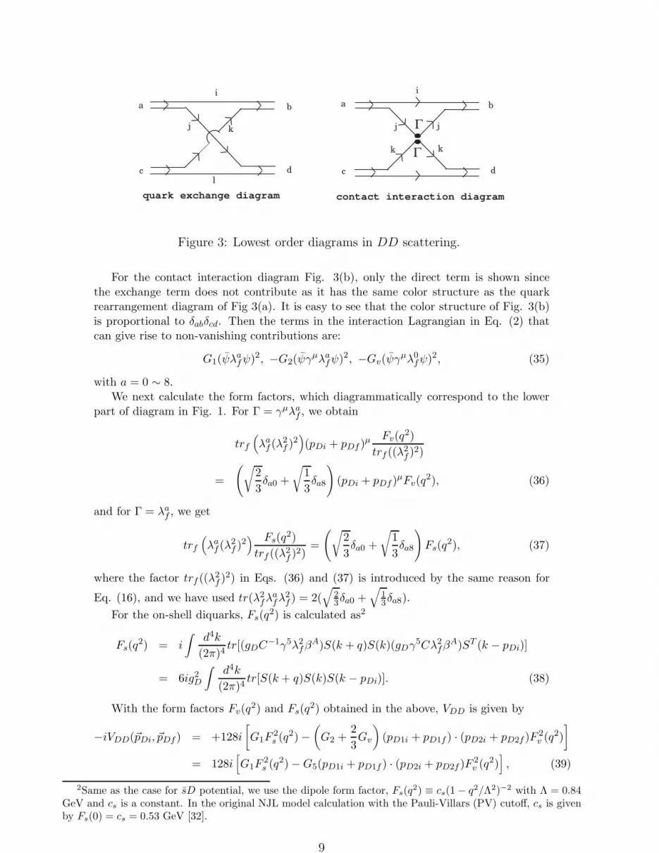
Figure 3: Lowest order diagrams in DD scattering.
For the contact interaction diagram Fig. 3(b), only the direct term is shown sincethe exchange term does not contribute as it has the same color structure as the quarkrearrangement diagram of Fig 3(a). It is easy to see that the color structure of Fig. 3(b)is proportional to δabδcd. Then the terms in the interaction Lagrangian in Eq. (2) thatcan give rise to non-vanishing contributions are:
G1(ψλafψ)2, −G2(ψγ
µλafψ)2, −Gv(ψγ
µλ0fψ)2, (35)
with a = 0 ∼ 8.We next calculate the form factors, which diagrammatically correspond to the lower
part of diagram in Fig. 1. For Γ = γµλaf , we obtain
trf(
λaf (λ2
f )2)
(pDi + pDf )µFv(q
2)
trf ((λ2f )2)
=
(
√
2
3δa0 +
√
1
3δa8
)
(pDi + pDf )µFv(q2), (36)
and for Γ = λaf , we get
trf(
λaf (λ2
f )2) Fs(q
2)
trf ((λ2f )2)
=
(
√
2
3δa0 +
√
1
3δa8
)
Fs(q2), (37)
where the factor trf ((λ2f )2) in Eqs. (36) and (37) is introduced by the same reason for
Eq. (16), and we have used tr(λ2fλ
afλ
2f ) = 2(
√
23δa0 +
√
13δa8).
For the on-shell diquarks, Fs(q2) is calculated as2
Fs(q2) = i
∫
d4k
(2π)4tr[(gDC
−1γ5λ2fβ
A)S(k + q)S(k)(gDγ5Cλ2
fβA)ST (k − pDi)]
= 6ig2D
∫
d4k
(2π)4tr[S(k + q)S(k)S(k − pDi)]. (38)
With the form factors Fv(q2) and Fs(q
2) obtained in the above, VDD is given by
−iVDD(~pDi, ~pDf ) = +128i
[
G1F2s (q2) −
(
G2 +2
3Gv
)
(pD1i + pD1f ) · (pD2i + pD2f )F 2v (q2)
]
= 128i[
G1F2s (q2) −G5(pD1i + pD1f ) · (pD2i + pD2f )F 2
v (q2)]
, (39)
2Same as the case for sD potential, we use the dipole form factor, Fs(q2) ≡ cs(1 − q2/Λ2)−2 with Λ = 0.84
GeV and cs is a constant. In the original NJL model calculation with the Pauli-Villars (PV) cutoff, cs is givenby Fs(0) = cs = 0.53 GeV [32].
9

where the factor +128i in a first line of Eq. (39) comes from the Wick contractions, andin a second line we have used the relation between couplling constants in meson sectors;G5 = G2 + 2
3Gv which is explained in section 2. The momenta of the diquarks in theinitial and final states in Fig. 4 are given by
pD1i(f) = (√s2/2, ~pDi(f)),
pD2i(f) = (√s2/2,−~pDi(f)), (40)
with q = pD1f − pD1i = pD2i − pD2f . s2 = 4(~p 2Di +M2
D) = 4(~p 2Df +M2
D) is the DD centerof mass energy squared.
= + DDtDD VDD VDD
P/2-p'
p
p
D1i
tD2i
pD1f
pD2f
P/2+p'
Figure 4: BS equation for DD.
As in the case of sD scattering, we use the BbS three-dimensional reduction schemeand the resulting equation for DD scattering reads as
tDD(~pDf , ~pDi) = VDD(~pDf , ~pDi)+
∫
d3p′
(2π)3VDD(~pDf , ~p
′
)GBbSDD (|~p ′ |, s2)tDD(~p
′
, ~pDi), (41)
with
GBbSDD (|~p ′ |, s2) =
1
4ED(|~p ′ |)(s2/4 − ED(|~p ′ |)2 + iǫ)
=1
4ED(|~p ′ |)(~p 2Df − ~p ′2 + iǫ)
, (42)
with ED(|~p ′ |) =√
~p ′2 +M2D.
In the JW model for Θ+, the diquark-diaquark spatial wave function must be anti-symmetric and we will consider here only the lowest configuration, namely, DD are inrelative p-wave. Partial wave expansion of Eq. (69) then gives
tl=1DD(pf , pi) = V l=1
DD (pf , pi) + 4π
∫
dp′
(2π)3p′2GBbS
DD (p′, s2)Vl=1DD (pf , p
′)tl=1DD(p′, pi), (43)
with pi(f) ≡ |~pDi(f)|, p′ ≡ |~p ′ |.
4 Relativistic Faddeev equation
4.1 3-body Lippmann-Schwinger equation
For a system of three particles with momenta ~k′is (i = 1, 2, 3), we introduce the Jacobimomenta with particle 3 as a special choice:
~k1 = µ1~P + ~p+ α1
~q3~k2 = µ2
~P − ~p+ α2~q3
~k3 = µ3~P + α3
~q3, (44)
10

with∑
µn = 1 and α3 = −α1 − α2. For the coefficients we find µn = mn/M , M =m1+m2+m3, and α1 = m1/m12, α2 = m2/m12, α3 = −1, where mij = mi+mj (i 6= j).In terms of the Jacobi momenta the total kinetic energy is given by:
Ktot =P 2
2M+
p 2
2m12+
q232m(12)3
, (45)
where m(ij)k = mkmij/M .New integration variables are chosen to be: p = fp3 p with fp3 =
√2m12 and q3 = fq3 q
with fq3 =√
2m(12)3, and in general for cyclic (ijk), fpi =√
2mjk and fqi =√
2m(jk)i.
In terms of the new integration variables we have
Ktot =P 2
2M+ p2 + q2, (46)
and the 3-body Lippmann-Schwinger equation for the T-matrix becomes:
T (~p, ~q) = V + fp33fq3
3∫
d3p′
(2π)3
∫
d3q′
(2π)3V G3(p
′, q′) T (~p ′, ~q ′), (47)
with G3(p, q) = 1/(z −Ktot). The parameter z is implicit in the arguments of T and G3
in Eq. (47), a convention to be followed hereafter.Similarly we define the Jacobi momenta ~pi, ~qi with particle i as the special choice. The
momenta are related to each other as
~pi = aij~pj + bij~qj, ~qi = cij~pj + dij~qj , (48)
where (ijk) are cyclic, and aij = −[mimj/(mi +mk)(mj +mk)]1/2, bij =
√
1 − a2ij = −bji,
cij = −bij and dij = aij .It can be shown that the total angular momentum is related to the angular momentum
~lpi and ~lqi by
~L =3∑
i=1
(
~ri × ~ki
)
=3∑
i=1
(
~lpi +~lqi
)
+~lc. (49)
With these three choices of Jacobi momenta we may introduce corresponding 3-particlestates | >n where particle n plays a special role. For the 3-particle T-matrix we have
< ~k1, ~k2, ~k3|T |α >=n< ~pn, ~qn|T |α >, (50)
or in terms of the Faddeev amplitudes Tn,
< ~k1, ~k2, ~k3|T |α >= T1(~p1, ~q1) + T2(~p2, ~q2) + T3(~p3, ~q3), (51)
with Tn(~pn, ~qn) =n< ~pn, ~qn|Tn|α >.For the pentaquark system we now chose particles 1 and 3 as the diquark and particle
2 to be the s. The Faddeev equations for T = T1+T2+T3 with Ti = ti+∑
j 6=itiG2(s)Tj (i =
1, 2, 3), with ti denoting the two-body t-matrix between particle pair (jk), become
T1(~p1, ~q1) = fp33fq3
3∫
d3p′3(2π)3
∫
d3q′3(2π)3
K13 G3(p′3, q
′3) T3(~p3
′, ~q3′)
+ fp23fq2
3∫
d3p′2(2π)3
∫
d3q′2(2π)3
K12 G3(p′2, q
′2) T2(~p2
′, ~q2′), (52)
where the channels 1 and 3 correspond to D(sD) states and channel 2 to the s(DD)states. Since diquarks obey Bose-Einstein statistics, we have T3(~p3, ~q3) = T1(−~p3, ~q3) and
11

T3(~p3, ~q3) = T1(−~p1, ~q1). We note that the symmetry property which requires the ampli-tude T be anti-symmetric with respect to interchange of the 2 diquarks is automaticallysatisfied by the angular momentum content L = lq1 = lp2 = 1, lp1 = lq2 = 0.
The s(DD) T-matrix T2 satisfies
T2(~p2, ~q2) = 2fp31fq
31
∫
d3p′1(2π)3
∫
d3q′1(2π)3
K21 G3(p′1, q
′1) T1(~p1
′, ~q1′). (53)
The kernels K13 and K12 are expressed in terms of the sD t-matrix
K13 = K12 = tsD(~p1, ~p1′; z − q21)
(2π)3
fq1
3δ(3)[~q1 − ~q1
′]. (54)
Similarly the kernel K21 is given by
K21 = tDD(~p2, ~p2′; z − q22)
(2π)3
fq2
3δ(3)[~q2 − ~q2
′]. (55)
The term with K13 can be worked out by making use of the δ-function relation
δ(3)[
~q1 − ~q1′] =
2
q1δ(
q21 − q′12)
δ(
cos θq3− cos θq′
3
)
δ(
φq′3− φq3
)
, (56)
and the linear relation ~q1′ = c13~p3
′ + d13~q3′, which lead to
δ(3)[
~q1 − ~q1′] =
1
q1c13d13p′3q
′3
δ
(
cos θp′3q′3− q′21 − c′213p
′23 − d2
13q′23
2c13d13p′3q
′3
)
× δ(
cos θq3− cos θq′
3
)
δ(
φq′3− φq3
)
. (57)
We mention that similar expression for a delta function in the term K12 can also beobtained by replacing 3 → 2.
Performing a partial wave expansion for the D(sD) amplitude
T1(~p1, ~q1) = 4πY ∗lp10(Ωp1
)Ylq10(Ωq1)TL
1 (p1, q1), (58)
and for the sD t-matrix tsD(~p1, ~p1′; z − q21),
tsD(~p1, ~p1′; z − q21) = 4πY ∗
lp10(Ωp1)Ylp10(Ωp′
1)t
(lp1)sD (p1, p
′1; z − q21), (59)
yield
TL1 (p1, q1)
= c3
∫ ∞
0q′3
2dq′3
∫ B13
A13
p′32dp′3 t
(lp1)sD (p1, p
′1; z − q21) X13
1
c13 d13 q1 p′3 q
′3
G3(p′3, q
′3) T
L3 (p′3, q
′3)
+c2
∫ ∞
0q′2
2dq′2
∫ B12
A12
p′22dp′2 t
(lp1)sD (p1, p
′1; z − q21) X12
1
c12 d12 q1 p′2 q′2
G3(p′2, q
′2) T
L2 (p′2, q
′2),
(60)
with
c3 =2√π
(fp3fq3/fq1)3, c2 =
2√π
(fp2fq2/fq1)3, (61)
and where the boundariesA,B for the p′ integration can easily be found from the conditionq21 = q′1
2 in Eq. (57), given by
Aij =
∣
∣
∣
∣
∣
cijq′j + qi
dij
∣
∣
∣
∣
∣
(62)
Bij =
∣
∣
∣
∣
∣
cijq′j − qi
dij
∣
∣
∣
∣
∣
, (63)
12

For the s(DD) amplitude T2, partical wave expansion gives,
TL2 (p2, q2) = 2c1
∫ ∞
0q′1
2dq′1
∫ B21
A21
p′12dp′1
× t(lp2)DD (p2, p
′2; z − q22) X21
1
c21 d21 q2 p′1 q′1
G3(p′1, q
′1) T
L1 (p′1, q
′1), (64)
where A21 and B21 are given by Eq. (63), and
c1 =2√π
(fp1fq1/fq2)3. (65)
In the above equations Xij are angular momentum functions depending on the stateswe consider. In our case, the sD 2-body channel is a s-wave, lp = 0, and the DD channela p-wave, lp = 1. Hence, for the 3-body channel with total angular momentum L = 1we have for the D(sD) 3-body channnel lp1 = 0, lq1 = L and lp3 = 0, lq3 = L, while fors(DD) lp2 = 1, lq2 = 0. The obtained Xij have the form
X13 =1
4π√
3Ylq30(θq3 q1
), X12 =1
4π√
3Ylq20(θq2 q1
), X21 =1
4π√
3Ylp20(θp2 p1
). (66)
4.2 Relativistic Faddeev equations
Following Amazadeh and Tjon [42] (see also [33]) we adopt the relativistic quasi-potentialprescription based on a dispersion relation in the 2-particle subsystem. Then the 3-bodyBethe-Salpeter-Faddeev equations have essentially the same form as the non relativisticversion.Taking the representation with particle 3 as special choice we may write down forthe 3-particle Green function a dispersion relation of the (1,2)-system, i.e.,
G3(p3, q3; s3) =E1(k1) + E2(k2)
E1(k1)E2(k2)
1
s3 − q23 − (E1(k1) + E2(k2))2, (67)
with E1(k1) =√
k21 +m2
1, E2(k2) =√
k22 +m2
2, and s3 = P 2 being the invariant 3-particleenergy square. In the 3-particle cm-system we have
√s3 = M +Eb. The resulting 2-body
Green function with invariant 2-body energy square s2 has then the form of the BSLTquasi-potential Green function
G2(p3; s2) =E1(k1) + E2(k2)
E1(k1)E2(k2)
1
s2 − (E1(k1) + E2(k2))2. (68)
This quasi-potential prescription for G3 has obviously the advantage that the 2-bodyt-matrix in the Faddeev kernel satisfies the same equation as the one in the 2-particleHilbert space with only a shift in the invariant 2-body energy. So the structure of theresulting 3-body equations are the same as in the non relativistic case.
5 Results and discussions
In the NJL model some cutoff scheme must be adopted since the NJL model is non-renormalizable. However, in this work we will not use any cutoff scheme but simplyemploy the dipole form factors for the scalar and vector vertices. Namely, the NJL modelis only used to study the Dirac, flavor and color structure of the sD and DD potentials.
For the values of the masses Mu,d, Ms and MD, we use the empirical values M = Mu =Md = 400 MeV and Ms = MD = 600 MeV [32]. We will treat the coupling constants
13

Gi (i = 1 ∼ 5) in Eq. (2) as free parameters. For the sD channel, it depends only onGv = G3 +G4 = 3
2 (G5 −G2) as seen in Eq. (16).In the NJL model calculation with the Pauli-Villars (PV) cutoff regularization [32],
the coupling constants Gπ, Gρ and Gω are related with the parameters used in our workby G1 = Gπ/2, G2 = Gρ/2 and G5 = Gω/2. Thus by using the values of mesonic couplingconstants in the NJL model, Gv is determined as Gv = 3
2(Gω/2 − Gρ/2) = 32(7.34/2 −
8.38/2) = −0.78 GeV−2. We remark that the sign of Gv is definitely negative sinceexperimentally omega meson is heavier than the rho meson. Then the interaction betweens and diquark in s-wave is attractive, as can be seen from the sD s-wave phaseshift shownin Fig. 5 with Gv = −0.78 GeV−2, while the interaction between s and diquark is repulsivewhich can be seen in Fig. 6. In both figures we find that the magnitudes of the phaseshiftis within 10 degrees, that is, Gv = −0.78 GeV−2 gives very weak interaction between s (s)and diquark. As we can see in Figs. 5 and 6, generally the phaseshift in s-wave is moresensitive to three momentum than that in p-wave. We note that sD and sD phaseshift arenot symmetric around the pE axis, which can be understood from the decompositions oftsD and tsD in the spinor space in appendix B. We further mention that if Gv is determinedfrom the Λ hyperon mass MΛ = 1116 MeV within the sD picture, one obtains Gv = 6.44GeV−2, which is different from Gv = −0.78 GeV−2 determined from meson sector in theNJL model in sign. In this case the rho meson mass is larger than the omega meson mass,that is, the vector meson masses are not correctly reproduced.
DD phaseshift is plotted in Fig. 7 where we have used the values of coupling constantsG1 = Gπ/2 = 5.21 GeV−2 and G5 = Gω/2 = 3.67 GeV−2 which are determined frommeson sectors in the NJL model calculation with the Pauli-Villars cutoff [32]. We caneasily see that the phaseshift δl is definitely negative i.e., the DD interaction is repulsive,and its dependence on three momentum pE is very strong and almost proportional to pE
both for s-wave and p-wave. This strong pE dependence of phaseshift comes from the p2E
dependence of a second term (pD1i + pD1f ) · (pD2i + pD2f ) in Eq. (39).The Gv dependence of the sD binding energy, EsD, is presented in Fig. 8. We find that
the sD bound state begins to appear around Gv = −5 ∼ −6 GeV−2, becomes more deeplybound as Gv becomes more negative. It is easily seen that EsD is almost proportionalto Gv . However even for the case of a weakly bound state with |EsD| less than 0.1 GeV,it will require a value of −Gv = 5 ∼ 6 GeV−2 which is about eight times larger thanthe −Gv determined from meson sector in the original NJL model with the PV cutoffregularization.
For the calculation of the pentaquark binding energy we use the relativistic three-bodyFaddeev equation which is introduced in section 4. If the pentaquark state is in JP = 1
2
+
state with which we are concerned in the present paper, the total force is attactive butthere is no pentaquark bound state.
On the other hand if the pentaquark state is in JP = 12−
state, a bound pentaquarkstate begins to appear when Gv becomes more negative than −8.0 GeV−2, a value in-consistent with what is required to predict a bound Λ hyperon with MΛ = 1116 MeV ina quark-diquark model as mentioned in Sec. 5. The lowest configuration which wouldcorrespond to a JP = 1
2
−state is for the spectator s to be in p−wave w.r.t. to a DD
pair in p−wave, or alternatively speaking, the spectator diquark in relative s-wave to sDin s-wave. Our results for the binding energy of a JP = 1
2
−pentaquark state for the
case with and without DD channel are given in Table 1. It is found that although theDD interaction is repulsive, including the DD channel gives an additional binding energywhich is leading to the more deeply pentaquark boundstate. It is because the couplingto the DD channel is attractive due to the sign of the effective kernel K21 in Eqs. (53,55). This depends on the recoupling coefficients X21, X12 in Eq. (66) and the 2-bodyt-matrices.
14

Gv[GeV−2] E0
B(5q)[MeV ] EB(5q)[MeV ]
-8.0 47 77
-9.0 87 139
-10.0 132 205
-12.0 226 333
-14.0 316 505
Table 1: The binding energy of JP = 12
−pentaquark state. E0
B(5q) (EB(5q)) is the bindingenergy without (including) the DD channel.
In Fig. 9 (10) the phaseshift of sD is plotted, where the coupling constant is fixedat Gv = −8.0 GeV−2 (Gv = −14.0 GeV−2). It is easily seen that in Figs. 9 and 10 thephaseshift of sD in s-wave is positive for small pE < 0.3 GeV and pE < 0.45 GeV, butit changes the sign around pE = 0.3 and pE = 0.45 GeV, thus the phaseshift of sD ins-wave is very sensitive to three momentum pE. Whereas the phaseshift of sD in p-waveis definitely positive.
In Fig. 11 we plot the phaseshift of sD with the coupling constant Gv = −14.0GeV−2 which is same as the one used in Fig. 10. Different from the phaseshift of sD thephaseshifts of sD in s and p-wave do not change the sign for higher three momentum pE ,i.e., the sign of the phaseshifts are definitely negative.
From the above results we find that even if we use a very strong coupling constant Gv
which is unphysical because it gives much larger mass difference of rho and omega mesonsthan the experimental value, Mω−Mρ = 13 MeV, it is impossible to obtain the pentaquark
bound state with JP = 12
+. With only the J = 1
2 three-body channels considered, we do
not find a bound JP = 12
+pentaquark state. The JP = 1
2
−channel is more attractive,
resulting in a bound pentaquark state in this channel, but for unphysically large valuesof vector mesonic coupling constants.
6 Summary
In this work, we have presented a Bethe-Salpeter-Faddeev (BSF) calculation for the pen-taquark Θ+ in the diquark picture of Jaffe and Wilczek in which Θ+ is treated as adiquark-diquark-s three-body system. The Blankenbecler-Sugar reduction scheme is usedto reduce the four-dimensional integral equation into three-dimensional ones. The two-body diquark-diquark and diquark-s interactions are obtained from the lowest order dia-grams prescribed by the Nambu-Jona-Lasinio (NJL) model. The coupling constants in theNJL model as determined from the meson sector are used. We find that sD interactionis attractive in s-wave while DD interaction is repulsive in p-wave. Within the truncatedconfiguration where DD and sD are restricted to p- and s-waves, respectively, we do notfind any bound 1
2+
pentaquark state, even if we turn off the repulsive DD interaction.It indicates that the attractive sD interaction is not strong enough to support a boundDDs system with JP = 1
2
+.
However, a bound pentaquark with JP = 12
−begins to appear if we change the vector
mesonic coupling constant Gv from −0.78 GeV−2, as determined from the mesonic sector,to around Gv = −8 GeV−2. And it becomes more deeply bound as Gv becomes morenegative.
15

Acknowledgements
This work was supported in part by the National Science Council of ROC under grant no.NSC93-2112-M002-004 (H.M. and S.N.Y.). J.A.T. wishes to acknowledge the financialsupport of NSC for a visiting chair professorship at the Physics Department of NTU andthe warm hospitality he received throughout the visit. K.T. acknowledges the supportfrom the Spanish Ministry of Education and Science, Reference Number: SAB2005-0059.
-20
-15
-10
-5
0
5
10
15
20
0 0.05 0.1 0.15 0.2 0.25 0.3 0.35 0.4 0.45 0.5
δ l [
deg]
pE [GeV]
Phaseshift of -sDS-waveP-wave
Figure 5: Three momentum pE dependence of the phaseshift δl for the sD interaction with thecoupling constant Gv = −0.78 GeV−2.
-20
-15
-10
-5
0
5
10
15
20
0 0.05 0.1 0.15 0.2 0.25 0.3 0.35 0.4 0.45 0.5
δ l [
deg]
pE [GeV]
Phaseshift of sDS-waveP-wave
Figure 6: Three momentum pE dependence of the phaseshift δl for the sD interaction with thecoupling constant Gv = −0.78 GeV−2.
16

-90
-80
-70
-60
-50
-40
-30
-20
-10
0
0 0.2 0.4 0.6 0.8 1
δ l [
deg]
pE [GeV]
Phaseshift of DDS-waveP-wave
Figure 7: Three momentum pE dependence of the phaseshift δl for the DD interaction.
0
0.05
0.1
0.15
0.2
0.25
0.3
0.35
0.4
0.45
0.5
6 8 10 12 14
-EB
(- sD)
[GeV
]
-Gv [GeV]
Figure 8: Gv dependence of the sD binding energy.
17

-80
-60
-40
-20
0
20
40
60
80
0 0.05 0.1 0.15 0.2 0.25 0.3 0.35 0.4 0.45 0.5
δ l [
deg]
pE [GeV]
Phaseshift of -sD, Gv=-8.0 GeV-2
S-waveP-wave
Figure 9: Three momentum pE dependence of the phaseshift δl for the sD interaction with thecoupling constant Gv = −8.0 GeV−2.
-80
-60
-40
-20
0
20
40
60
80
0 0.05 0.1 0.15 0.2 0.25 0.3 0.35 0.4 0.45 0.5
δ l [
deg]
pE [GeV]
Phaseshift of -sD, Gv=-14.0 GeV-2
S-waveP-wave
Figure 10: Three momentum pE dependence of the phaseshift δl for the sD interaction withthe coupling constant Gv = −14.0 GeV−2.
18

-40
-20
0
20
40
0 0.05 0.1 0.15 0.2 0.25 0.3 0.35 0.4 0.45 0.5
δ l [
deg]
pE [GeV]
Phaseshift of sDS-waveP-wave
Figure 11: Three momentum p dependence of the phaseshift δl for the sD interaction with thecoupling constant Gv = −14.0 GeV−2
Appendices
A Partial wave expansion
In the 2-body center of mass frame the partial wave expansion is defined by
t(~pf , ~pi) =∑
l
2l + 1
4πPl(cosθpipf
) < pf l|t|pil >
≡∑
l
(2l + 1)Pl(cosθpipf)tl(|~pf |, |~pi|), (69)
with ~pi(f) ≡ ~p 1i(f) = −~p 2i(f). Then tl(|~pf |, |~pi|) in Eq. (69) is written in terms of t(~pf , ~pi)by
tl(|~pf |, |~pi|) =1
2
∫ 1
−1dcosθpipf
Pl(cosθpipf)t(~pf , ~pi). (70)
The phase shift δl is given by
tl(p, p) = −8π√s2
peiδlsinδl, (71)
where p ≡ |~p1i| = |~p2i| = |~p1f | = |~p2f | and s2 = (p1i + p2i)2 = (p1f + p2f )2.
B The results for Vs(s)D,nm and Ks(s)D,nm (n, m = 1, 2)
In this appendix we show the results for Vs(s)D,nm and Ks(s)D,nm (n,m = 1, 2) defined inEqs. (28-31):
VsD,11(pDi, pDf , x) =p0
Di + p0Df
2,
19

VsD,12(pDi, pDf , x) = −pDf + xpDi
2= −psf + xpsi
2,
VsD,21(pDi, pDf , x) =pDi + xpDf
2=psi + xpsf
2,
VsD,22(pDi, pDf , x) =x
2(p0
Di + p0Df ),
and
KsD,11(pDi, p′D, xi) =
1
2
[
(p0Di + p
′0D)Ms + (
√s2 − p
′0D)(p
′0D + p0
Di) + p′2D + xip
′DpDi
]
,
KsD,12(pDi, p′D, xi) = −1
2
[
(p′D + xipDi)(Ms −√s2 + p
′0D) − p′D(p0
Di + p′0D)]
,
KsD,21(pDi, p′D, xi) =
1
2
[
(pDi + xip′D)(Ms +
√s2 − p
′0D) + xip
′D(p0
Di + p′0D)]
,
KsD,22(pDi, p′D, xi) = −1
2
[
xiMs(p0Di + p
′0D) − (pDip
′D + xip
′2D) + xi(p
′0D −√
s2)(p0Di + p
′0D)]
,
where x ≡ pDi · pDf , xi ≡ pDi · p′
D.VsD,nm and KsD,nm are related with VsD,nm and KsD,nm by
VsD,nm(p, q, xpq) = −VsD,nm(p, q, xpq),
KsD,nm(p, q, xpq) = −KsD,nm(p, q, xpq).
C Parametrizations for tsD and tsD
tsD can be parametrized as
tsD(pDi, pDf ) =∑
ρ,ρ′=±Λρ
[
F ρρ′
S + F ρρ′
T iσµνpµDfp
νDi
]
Λρ′ , (72)
where Λ± = 1±γ0
2 . Components of tsD is written as
tsD(pDi, pDf ) =
(
F++S + F++
T i~σ · ~n F+−T ~σ · ~v
F−+T ~σ · ~v F−−
S + F−−T i~σ · ~n
)
, (73)
where ~n = ~pDf × ~pDi, ~v = p0Df~pDi − p0
Di~pDf , and ± means upper and lower componentsin the spinor space i.e., (tsD)ρ,ρ′ = ΛρtsDΛρ′ .
The decomposition into upper and lower components in eq. (30) for tsD gives
tsD,11(pDi, pDf ) = −F−−S ,
tsD,12(pDi, pDf ) = −F−+T (xp0
DfpDi − p0DipDf ),
tsD,21(pDi, pDf ) = −F+−T (p0
DfpDi − xp0DipDf ),
tsD,22(pDi, pDf ) = −F++T pDipDf (x2 − 1).
We can parametrize tsD in the same way (= eq. (72))
tsD(pDf , pDi) =∑
ρ,ρ′=±Λρ
[
F ρρ′
S + F ρρ′
T iσµνpµDfp
νDi
]
Λρ′ , (74)
where Λ± = 1±γ0
2 .Similar to tsD the decomposition into upper and lower components by eq. (28) gives
tsD,11(pDf , pDi) = F++S ,
tsD,12(pDf , pDi) = F+−T (p0
DfpDi − xp0DipDf ),
tsD,21(pDf , pDi) = F−+T (xp0
DfpDi − p0DipDf ),
tsD,22(pDf , pDi) = F−−T pDipDf (x2 − 1).
20

References
[1] T. Nakano et al. [LEPS Collaboration], Phys. Rev. Lett. 91, (2003) 012002.
[2] S. Stepanyan et al. [CLAS Collaboration], Phys. Rev. Lett. 91, (2003)252001.
[3] D. Diakonov, V. Petrov and M.V. Polyakov, Z. Phys. A359, (1997) 305.
[4] S. Eidelman et al. [Particle Data Group Collaboration], Phys. Lett. B592, (2004) 1;W.-M. Yao [PDG], J. Phys.G33, (2006) 1.
[5] K.T. Knopfle, M. Zavertyaev and T. Zivko [HERA-B Collaboration], J. Phys. G30
(2004) S1363.
[6] K. Abe et al., [BELLE Collaboration], hep-ex/0411005.
[7] A. Raval (on behalf of the H1 and ZEUS Collaborations), Nucl. Phys. Suppl. B164
(2007) 113.
[8] Y.M. Antipov et al., [SPHINX Collaboration] Eur. Phys. J. A21 (2004) 455.
[9] M. Battaglieri et al. [CLAS Collaboration], Phys. Rev. Lett. 96 (2006) 042001.
[10] K. Abe et al., [BELLE Collaboration], Phys. Lett. B632 (2006) 173.
[11] K. Hicks, Proc. IXth Int’l Conference on Hypernuclear and Strange Particle Physics,Mainz, Germany, Oct. 10-14, 2006, hep-ph/0703004.
[12] S.V. Chekanov and B.B. Levchenko, hep-ph/0707.2203.
[13] F. Stancu and D.O. Riska, Phys. Lett. B575 (2003) 242.
[14] F. Stancu, Phys. Lett. B595 (2004) 269.
[15] T. Kojo, A. Hayashigaki and D. Jido, Phys. Rev. C74 (2006) 045206.
[16] F. Csikor, Z. Fodor, S.D. Katz and T.G. Kovacs, JHEP 11 (2003) 070; F. Csikor, Z.Fodor, S.D. Katz, T.G. Kovacs and B.C. Toth, Phys. Rev. D73 (2006) 034506; S.Sasaki, Phys. Rev. Lett. 93 (2004) 152001.
[17] M. Oka, Prog. Theor. Phys. 112, (2004) 1.
[18] R.L. Jaffe, Phys. Rept. 409, (2005) 1.
[19] R.L. Jaffe and F. Wilczek, Phys. Rev. Lett. 91, (2003) 232003.
[20] M. Ida and Kobayashi, Prog. Theor. Phys. 36, (1966) 846; D.B. Lichtenberg and L.J.Tassie, Phys. Rev. 155, (1967) 1601.
[21] R.L. Jaffe and K. Johnson, Phys. Lett. B60, (1976) 201; R.L. Jaffe, Phys. Rev. D14,(1977) 267, 281.
[22] For a review and further references, M. Anselmino, E. Predazzi, S. Ekelin, S. Fredriks-son, and D.B. Lichtenberg, Rev. Mod. Phys. 65, (1993) 1199.
[23] Y. Nambu and G. Jona-Lasinio, Phys. Rev. 122, 345 (1960); 124, 246 (1961).
[24] C.G. Callan Jr. and R. Dashen, Phys. Rev. D17, (1978) 2717.
[25] S.P. Klevansky, Rev. Mod. Phys. 64, (1992) 649.
[26] M. Takizawa, K. Tsushima, Y. Kohyama, and K. Kubodera, Nucl. Phys. A507,(1990) 611.
[27] S. Huang and J. Tjon, Phys. Rev. C49, 1702 (1994).
[28] N. Ishii, W. Bentz and K. Yazaki, Nucl. Phys. A587, 617 (1995).
[29] H. Asami, N. Ishii, W. Bentz, and K. Yazaki, Phys. Rev. C 51, 3388 (1995).
21

[30] A. Buck, R. Alkofer and H. Reinhardt, Phys. Lett. B286, 29 (1992).
[31] H. Mineo, W. Bentz and K. Yazaki, Phys. Rev. C60, 065201 (1999); Nucl. Phys.A703, 785 (2002).
[32] H. Mineo, S.N. Yang, C.Y. Cheung and W. Bentz, Phys. Rev. C72, (2005) 025202.
[33] G. Rupp and J.A. Tjon, Phys. Rev. C37, (1988) 1729.
[34] R. Blankenbeckler and R. Sugar, Phys. Rev. 142, (1996) 1051.
[35] S. Klimt, M. Lutz, U. Vogl and W. Weise, Nucl. Phys. A516, (1990) 429; U. Vogl,M. Lutz, S. Klimt and W. Weise, Nucl. Phys. A516, (1990) 469.
[36] U. Vogl and W. Weise, Prog. Part. Nucl. Phys. 27, (1991) 195.
[37] N. Ishii, W. Bentz and K. Yazaki, Nucl. Phys. A587, (1995) 617.
[38] C.T. Hung, S.N. Yang, and T.-S.H. Lee, Phys. Rev. C64, (2001) 034309.
[39] S.Z. Huang and J. Tjon, Phys. Rev. C49, (1994) 1702.
[40] M. Oettel, G. Hellstern, R. Alkofer and H. Reinhardt, Phys. Rev. C58, (1998) 2459.
[41] J.L. Gammel, M.T. Menzel and W.R. Wortman, Phys. Rev. D3, (1971) 2175.
[42] A. Ahmadzadeh and J. Tjon, Phys. Rev. 147, (1966) 1111.
22


