FDI Technology Spillovers, Geography, and Spatial Diffusion

Mi Lina and Yum K. Kwanb

a University of Lincoln b City University of Hong Kong

This version: 06 July 2015 Abstract: This paper investigates the geographic extent of FDI technology spillovers and associated

spatial diffusion. By adopting a spatiotemporal autoregressive panel model as the platform of our study,

the complex impact resulting from FDI penetration is separated into spatial direct and indirect effect

while accounting for feedback loops among regions. A set of spatially partitioned summary measures is

produced to identify and to quantify FDI spillovers from different channels with distinct geographic

scopes. Empirical results based on data from China document that the direct impacts of FDI presence to a

specific location itself are likely to be negative. Domestic firms mainly benefit from FDI presence in their

neighboring regions through knowledge spillovers that have wider geographic scope. Negative market

stealing effect nevertheless has no spatial boundary. Policy implications of these findings are discussed.

Key Words: FDI spillovers, spatial diffusion, spatial dynamic panel, Chinese economy. JEL Classification: R12, F21, O33.

* We would like to thank Professors Cheng Hsiao, Chia-Hui Lu, Eden S.H. Yu, Larry Qiu, and seminar participants at City University of Hong Kong, University of Waterloo, Wilfred Laurier University, University of Lincoln, and conference participants of The 24th CEA (UK) and 5th CEA (Europe) Annual Conference (The Hague, 2013) and International Conference on Economic Linkages through International Trade, Investment, Migration and Tourism (Chu Hai College of Higher Education of Hong Kong, 2015) for helpful comments and suggestions. All remaining errors are our own. This work is supported by the Research Center of International Economics of City University of Hong Kong (Project No. 7010009). Correspondence: Mi Lin, Lincoln Business School, University of Lincoln. Email address: linmixm@gmail.com.  

FDI Technology Spillovers, Geography, and Spatial Diffusion Abstract: This paper investigates the geographic extent of FDI technology spillovers and

associated spatial diffusion. By adopting a spatiotemporal autoregressive panel model as the

platform of our study, the complex impact resulting from FDI penetration is separated into spatial

direct and indirect effect while accounting for feedback loops among regions. A set of spatially

partitioned summary measures is produced to identify and to quantify FDI spillovers from different

channels with distinct geographic scopes. Empirical results based on data from China document that

the direct impacts of FDI presence to a specific location itself are likely to be negative. Domestic

firms mainly benefit from FDI presence in their neighboring regions through knowledge spillovers

that have wider geographic scope. Negative market stealing effect nevertheless has no spatial

boundary. Policy implications of these findings are discussed.

Key Words: FDI spillovers, spatial diffusion, spatial dynamic panel, Chinese economy. JEL Classification: R12, F21, O33.

 

1

1. Introduction

Firms tend to agglomerate in specific areas so as to reduce transaction cost and exploit external

economies. Such external economies are commonly known as Marshallian externalities of which

the central idea highlights that the concentration of production in a particular location generates

external benefits for firms in that location through knowledge spillovers, labor pooling, and close

proximity of specialized suppliers (Marshall, 1920).1 The foreign direct investment (FDI) location

literature has documented similar self-perpetuating growth or agglomeration pattern of

multinational corporations (MNCs) in space and over time (see, among others, Head et al., 1995;

Cheng and Kwan, 2000a, 2000b; Blonigen et al., 2005; Lin and Kwan, 2011). The externalities

arising from FDI penetration also have long received great attentions from both economists and

policy makers. Although the previous literature has provided some evidence of FDI spillovers at

both firm and industry level (Lin et al., 2009; Abraham et al., 2010; Hale and Long, 2011; Xu and

Sheng, 2012; Damijan et al., 2013; Merlevede et al., 2014; among other earlier contributions), little

is known about the extent to which the regional presence of FDI affects the aggregate productivity

of local private firms in spatial dimension. This paper studies FDI spatial spillovers using county-

level data supplemented with precise GPS information of China. More specifically, this paper asks:

Do domestic private firms benefit from FDI presence in their local and neighbouring regions? How

to identify and quantify the geographic extent of FDI spillovers? Do FDI spillovers attenuate with

distance? If so, how rapid is the geographic attenuation pattern?

There exists a vast literature on FDI spillovers. FDI presence may benefit domestic firms via

channels like labor turnover, demonstration of new technology, competition effect, reverse

engineering, and ‘learning by watching’ (see, among others, MacDougall, 1960; Kokko, 1994;

Blalock and Gerlter, 2008). FDI spillovers from MNCs to domestic firms can also be negative. A

leading example is ‘market stealing effect’ (Aitken and Harrison, 1999), which argues that, in the

short run, indigenous firms may be constrained by high fixed cost that prevents them from reducing

their total cost; therefore, foreign firms with cost advantages due to better technology can steal

market share from domestic firms via price competition. As a result, due to a lack of economies of

scale, the shrinking demand will push up the unit cost of domestic firms and decrease their

operation efficiency. Consequently, while the penetration of MNCs may bestow positive

externalities on domestic firms, it could also generate, at the same time, a negative demand effect,

which drags down the productivity of local firms. Another possible source of negative impact                                                                                                                1 Marshall (1920) argues that firms can benefit from two types of external economies: 1) economies arising from ‘the

use of specialized skill and machinery’ which depend on ‘the aggregate volume of production in the neighborhood’ and 2) economies “connected with the growth of knowledge and the progress of the arts” which tie to the ‘aggregate volume of production in the whole civilized world’.

 

2

comes from foreign firms poaching local talents from domestic firms to the detriment of domestic

firms’ productivity (Blalock and Gerlter, 2008). The net impact from FDI presence on domestic

firms hence depends on the magnitude of these two opposite externalities.

Though the theoretical arguments are well established, the empirical literature so far provides

mixed evidence of the existence, the sign, and the magnitude of FDI spillovers. This is partially due

to the fact that the above mentioned channels are operative at the same time even though their

impacts may have different scopes and they reach local firms in different manners. Empirical

exercises focusing on simple association between domestic firms’ productivity and FDI presence

can at best summarize an averaged or mixed impact resulting from various channels and

dimensions, but it can barely reveal the underlying mechanism of FDI spillovers. Focusing

predominantly on this averaged impact will likely dilute the genuine and rich variations of FDI

spillovers and result in misleading conclusion. Identification problem thus remains a challenging

but vital issue in the FDI spillovers literature.

In this paper, we use geography to identify and quantify FDI spillovers. Geographical distance

determines the costs and the attenuation pattern of technology diffusion, which may reduce the

likelihood for indigenous firms that are distant from MNCs to expropriate spillovers. The fact that

spatial interactions are shaped by feedback loops (i.e., from one location to its neighbors, and then

neighbors’ neighbors, and finally back to the original location indirectly) further complicates the

identification issue and the interpretation of resulting estimates. Our method described in section 3

is capable of quantifying separately the direct and indirect impacts, as well as producing a set of

partitioning summary measures to describe the rate of decay pattern over space and time. Further,

we exploit the fact that different spillover channels should have different geographic scopes to

identify spillovers from different sources. For instance, it is reasonable to expect positive

knowledge spillovers should have a wider geographic scope than negative poaching effect, though

both are intermediated via the labor turnover channel. In view of the rapid development in modern

information technology, the diffusion barrier and communication cost for knowledge spillovers

have been significantly reduced. Labor mobility across regions, however, is still subject to high

reallocation expenses that increase with distance. It is thus more difficult for MNCs to poach talents

from distant domestic firms, implying that poaching effect should decay relatively faster.

Consequently, knowledge spillovers can be identified with wider geographic scope, whereas

poaching effect can be identified with more local scope. Negative market stealing effect, on the

other hand, should have no boundary as its impact could easily spread out to the whole country

through integrated markets. Given the increasingly diverse and convenient distribution channels for

 

3

products, sales network nowadays is hard to be segmented. Market stealing impact hence should

appear not just locally but also in wide geographic scope. Our empirical findings confirm the above

conjectures. Negative poaching effect in our estimations appears only in low-order spatial loops

while positive knowledge spillovers become dominant in wider geographic scope (high-order

spatial loops). Negative market stealing effect, however, is always quantitatively significant

regardless of geographic scope.

Many analyses in previous literature treat each region in the sample to be an isolated entity. The

role of spatial dependence is neglected, even though inter-regional knowledge spillovers across

regions have been identified, both theoretically and empirically, as an important factor in the

process of productivity growth (Rey and Montouri, 1999; Madriaga and Poncet, 2007).

Econometically speaking, it is well known that ignoring spatial factors in estimation could result in

misspecification and identification problems when these factors actually exist (Anselin, 2001;

Abreu et al., 2005). There are also strong theoretical reasons why regional total factor productivities

(TFPs) might be spatially correlated. Ciccone and Hall (1996) prove theoretically that the density of

economic activity (defined as intensity of labor, human, and physical capital relative to physical

space) would affect productivity in spatial dimension through externalities and increasing returns.

They also provide empirical evidence showing that more than half of the variance of productivity

across U.S. states can be attributed to the differences in the spatial density of economic activity.

Section 2 of this paper provides exploratory spatial analysis of our data, in which we will present in

detail the evidence of spatial autocorrelation for regional TFPs in China.

While a common theme in the existing literature is that agglomeration promotes spatial spillovers,

the direction of the association between geographical distance and spillovers, however, is not as

clear as one would expect. Backed by the argument that the exchange of tacit knowledge requires

face-to-face contacts, Audretsch and Feldman (1996) and Gertler (2003) emphasize that knowledge

sharing is highly sensitive to geographical distance and geographical proximity would promote

knowledge spillovers. Boschma and Frenken (2010), nevertheless, propose the so-called proximity

paradox, i.e., though geographical proximity may be a crucial condition for economic agents to

interact and to exchange knowledge, too much proximity between these agents in other dimensions

might actually decrease their operational efficiency. In the context of current paper, while

geographical proximity increases the likelihood of knowledge sharing between domestic private

firms and MNCs, proximities in the market they serve (Aitken and Harrison, 1999), the common

input markets they share, their knowledge bases, and their organizational proximity (Boschma and

Frenken, 2010) may also result in negative impact on the productivity performance of domestic

 

4

private firms. Our empirical results document strong evidence of proximity paradox in the context

of FDI penetration. FDI spillovers to domestic firms in the same locality are negative regardless of

spillover channels.

We employ two proxies to capture FDI spillovers in this paper. Many recent studies emphasize the

role of labor market pooling in the process of spatial knowledge spillovers. Fallick et al. (2006) and

Freedman (2008) illustrate that industry co-agglomeration facilitates labor mobility (moving among

jobs). Ellison et al. (2010) further document that industries employing the same types of workers

tend to co-agglomerate. Duranton and Puga (2004) explore the micro-foundations based on spatial

externalities arising from sharing, matching and learning among individuals. Kloosterman (2008)

and Ibrahim et al. (2009) both argue that industry agglomeration promote knowledge spillovers

since it facilitates individuals to share ideas and tacit knowledge. In line with these studies, we

adopt regional employment share of foreign firms as one of the proxies for FDI spatial spillovers in

this paper to capture spillovers from labor market pooling. To capture the potential pecuniary

externalities suggested by Aitken and Harrison (1999) (such as market stealing or crowding out of

local firms) we also use regional sales income share of foreign firms as the second proxy.

The focus of this paper is to identify and quantify FDI spillovers in spatial dimension. With the

presence of spatial interaction terms among the regressors, we show in section 3 that the marginal

impact of a regressor on the dependent variable is no longer the associated regression parameter.

Rather, the marginal impact is a highly nonlinear function of the regression parameters and spatial

weight matrix. Point estimates of the above mentioned proxies in our benchmark model are thus of

less interests, given also that they capture mixed impacts resulting from various factors operating

simultaneously. These point estimates should be interpreted with caution. Section 3 of our paper

discusses in detail these complications, as well as our approach to address these empirical issues.

The regional presence of FDI is largely driven by the related policy in China. With an aim of

facilitating local firms to learn from nearby MNCs, five Special Economic Zones (SEZs) were set

up in the early 1980s to attract foreign capital by exempting MNCs from taxes and regulations.2

These five special economic zones are Shenzhen, Xiamen, Hainan, Zhuhai, and Shantou, which are

all located in coastal areas. In view of the early success of this experiment, similar schemes, such as

Open Coastal Cities (OCCs), Open Coastal Areas, Economic and Technological Development

Zones (ETDZs) and Hi-Tech Parks, were set up subsequently to cover broader and inner regions in

                                                                                                               2 Commonly known as the strategy of ‘swapping market access for technology’.

 

5

the later years.3 Figure 1 compares the FDI spatial density distribution (measured as fixed asset

share of FDI in a specific county) between 1998 and 2007. As shown in the graphs, FDI presence in

1998 mainly clusters in coastal and some central regions of China. The graph for 2007 indicates that

the clustering pattern has been getting stronger over time. While the majority of clusters remain in

coastal and central regions, FDI presence has been directed and spread to broader and inner areas in

China. In view of the fact that similar place-based strategy has been widely implemented in the rest

of the world, our empirical results also generate important implications on the experiment of policy-

driven clustering among indigenous firms and MNEs in developing countries.

[Insert Figure 1 here]

The rest of this paper is organized as follows. Section 2 describes the data and presents the results

of exploratory spatial data analyses. Section 3 presents a spatial dynamic panel model that

incorporates the spatial features observed section 2. Section 4 discusses various econometric issues

and presents empirical results. The final section concludes with a summary and suggestions for

future research.

2. Data and Exploratory Data Analysis

2.1 Data

Data employed in this paper come from the annual census of above-size manufacturing firms of

China from 1998 to 2007. The National Bureau of Statistics (NBS) of China conducts the census.

The database (known as the Chinese Industrial Enterprises Database, NBS-CIE database

henceforth) reports census data for Chinese manufacturing firms with annual sales revenue over 5

million RMB. There are several variables (including the Chinese standard location indicator,

province code, city code, county code, district code, as well as firms’ full address) can help us

identify the location of a firm. Of all these variables, province code, city code and county code are

most complete and consistent over the years. Information specifying the distance between

individual firms is not available. We hence define ‘region’ as a county in this paper. Consequently,

all variables in this paper are aggregate county-level data constructed from firm-level information.

This results in an unbalanced panel data set with 1357 counties in 1998 and 2023 counties in 2007,

                                                                                                               3 See Cheng (1994) for detailed review of the evolution of FDI policy in China.

 

6

respectively. The longitude and latitude information of the counties are obtained from the GADM

database of Global Administrative Areas.4

Domestic private firms in this paper are defined as firms that have not received equity capital from

foreign investors or from any level of China’s government.5 Appendix A reports the information of

firms’ ownership structures and their proportions in each year in the database. More specifically, in

this paper, domestic private firms are firms with ownership structures from column (1) to column

(7) in the table. FDI firms correspond to columns of ‘Foreign Firms’ and ‘Sino-Foreign Joint

Ventures’.

The first step of our data analysis is to estimate total factor productivity (TFP) at firm level and then

aggregate them up to the county level for later spatial econometric analysis. In Appendices B and C,

we describe in details our data cleaning process and the procedure of constructing county-level TFP

from firm-level data.

2.2 Exploratory Spatial Data Analysis

In this section we present exploratory analysis of our data. Our focus is to present and reveal the

salient features of spatial autocorrelation for the variable of interest, i.e., county level TFP of

domestic private firms in China. By definition spatial autocorrelation describes the coincidence of

value similarity with locational similarity (Anselin, 2001). Positive spatial autocorrelation means

high (or low) values of a variable tend to cluster together in space, and negative spatial

autocorrelation indicates high (low) values are surrounded by low (high) values. As standard

measures, both global and local Moran’s I statistics are commonly adopted in the literature to

measure the strength and significance of spatial autocorrelation. Global Moran’s I statistic is

defined as

1 1

20

1

( )( )

( )

n n

ij it t jt ti j

t n

it ti

w x xnIS x

µ µ

µ

= =

=

− −=

−

∑∑

∑ (1)

                                                                                                               4 GADM is a spatial database of the location of the world’s administrative areas (or administrative boundaries). The

database describes where these administrative areas are (the spatial features), and for each area it provides some attributes, such as the name, geography area, longitude and latitude, and shape. Source: http://www.diva-gis.org/.

5 This study does not attempt to address and evaluate the impact of FDI on the productivity of China’s state-owned enterprises. This issue may be investigated in future research.

 

7

where itx is the variable of interest (TFP) for county i at time t; tµ is the mean of variable x in

year t; ijw is a spatial weight that depicts the relative similarity of two localities (counties i and j )

in space. n is the number of counties. 0S is a scalar factor equal to the sum of all ijw . In this paper,

we define the spatial weight as inversed geographical distance between two localities, i.e.,

1 ( )

0ij

ij

if i jdw

if i j

− ≠⎧= ⎨ =⎩

(2)

where ijd denotes the geographical distance between counties i and j .

Similarly, local Moran’s I statistic is defined as

2

1, 1,2 22

( ) ( ) ( ) where .

1

n n

it t ij jt t jt tj j i j j i

it i ti

x w x xI S

S n

µ µ µµ= ≠ = ≠

− − −= = −

−

∑ ∑ (3)

Local Moran’s I is an example of Local Indicators of Spatial Association (LISA) defined in Anselin

(1995).

By comparing equations (1) and (3), it can be shown that, for a row standardized weights matrix,

the global Moran’s I equals the mean of the local Moran’s I statistics up to a scaling constant.

Consequently, while local Moran’s I statistics describe the extent of significant spatial clustering of

similar values around each particular locality (county i ), global Moran’s I yields one statistic to

summarize these local information across the whole study area. For both global and local Moran’s I,

a positive value for I statistic indicates that a county has neighboring counties with similarly high or

low attribute values (TFP), i.e., this county is part of a cluster. A negative value for I statistic

indicates that a county has neighboring counties with dissimilar values, i.e., this county is an

outlier.6

Table 1 reports the global Moran’s I statistics for aggregate county level TFP for domestic private

firms. As shown in the table, Moran’s I statistics are significant and positive in all cases, indicating

positive spatial autocorrelation for TFP. Notice that the magnitude of the statistics increases

significantly over time, indicating an escalating pattern of spatial clustering in terms of TFP

innovation for domestic private firms during the sample period. This observation motives us to

                                                                                                               6 Both local and global Moran’s I statistics require the underlying variable to be normally distributed. We apply the

Shapiro and Francia (1972) normality test to both TFP level and growth rate. At the 5% significance level, the null hypothesis of normal distribution cannot be rejected.

 

8

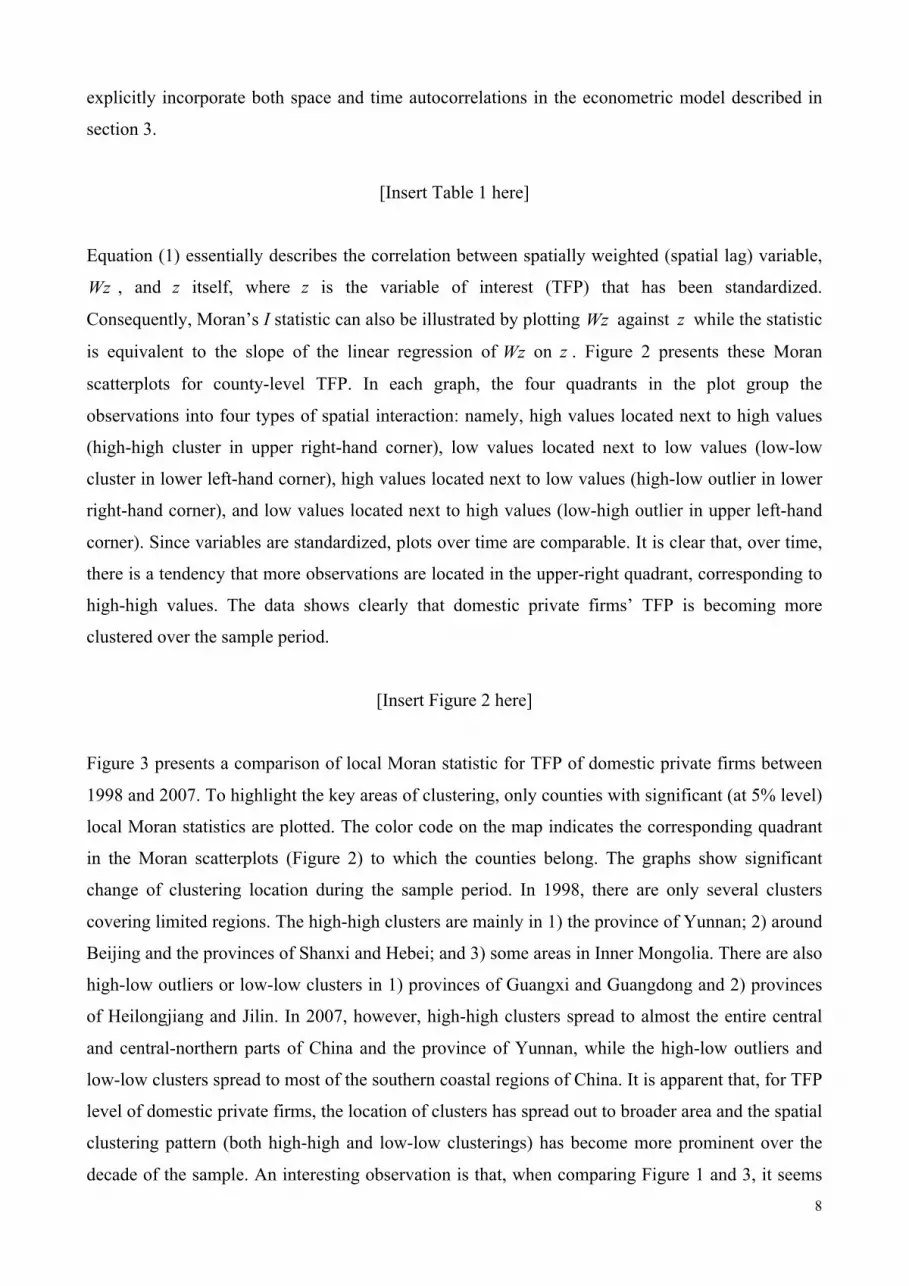
explicitly incorporate both space and time autocorrelations in the econometric model described in

section 3.

[Insert Table 1 here]

Equation (1) essentially describes the correlation between spatially weighted (spatial lag) variable,

Wz , and z itself, where z is the variable of interest (TFP) that has been standardized.

Consequently, Moran’s I statistic can also be illustrated by plotting Wz against z while the statistic

is equivalent to the slope of the linear regression of Wz on z . Figure 2 presents these Moran

scatterplots for county-level TFP. In each graph, the four quadrants in the plot group the

observations into four types of spatial interaction: namely, high values located next to high values

(high-high cluster in upper right-hand corner), low values located next to low values (low-low

cluster in lower left-hand corner), high values located next to low values (high-low outlier in lower

right-hand corner), and low values located next to high values (low-high outlier in upper left-hand

corner). Since variables are standardized, plots over time are comparable. It is clear that, over time,

there is a tendency that more observations are located in the upper-right quadrant, corresponding to

high-high values. The data shows clearly that domestic private firms’ TFP is becoming more

clustered over the sample period.

[Insert Figure 2 here]

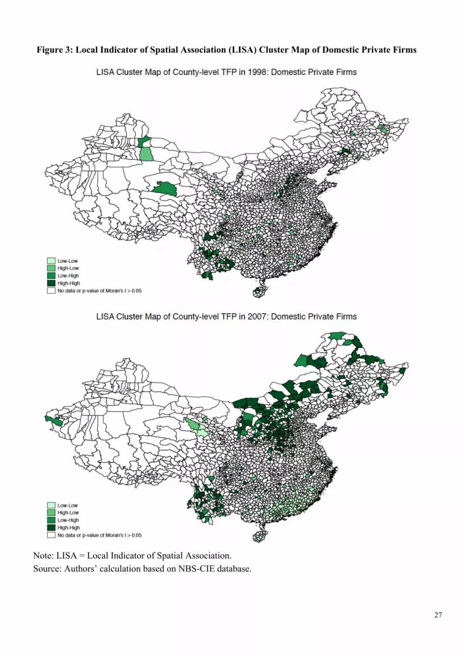
Figure 3 presents a comparison of local Moran statistic for TFP of domestic private firms between

1998 and 2007. To highlight the key areas of clustering, only counties with significant (at 5% level)

local Moran statistics are plotted. The color code on the map indicates the corresponding quadrant

in the Moran scatterplots (Figure 2) to which the counties belong. The graphs show significant

change of clustering location during the sample period. In 1998, there are only several clusters

covering limited regions. The high-high clusters are mainly in 1) the province of Yunnan; 2) around

Beijing and the provinces of Shanxi and Hebei; and 3) some areas in Inner Mongolia. There are also

high-low outliers or low-low clusters in 1) provinces of Guangxi and Guangdong and 2) provinces

of Heilongjiang and Jilin. In 2007, however, high-high clusters spread to almost the entire central

and central-northern parts of China and the province of Yunnan, while the high-low outliers and

low-low clusters spread to most of the southern coastal regions of China. It is apparent that, for TFP

level of domestic private firms, the location of clusters has spread out to broader area and the spatial

clustering pattern (both high-high and low-low clusterings) has become more prominent over the

decade of the sample. An interesting observation is that, when comparing Figure 1 and 3, it seems

 

9

that areas with high-high clustering of domestic private firms’s TFP are also areas with low FDI

density, while areas with low-low clustering are areas with high FDI density.

[Insert Figure 3 here]

To sum up, exploratory spatial data analysis reveals salient spatial autocorrelation feature for

county-level TFP of domestic private firms. There is a strong tendency that TFPs are getting more

clustered throughout the sample period. In the next section, we further explore these observations in

a spatiotemporal model that incorporates both spatial interactions across regions and spatial

technology diffusion of FDI.

3. The Empirical Model

To estimate the extent of FDI spillovers and its diffusion pattern over time and across space, we

generalize the spatiotemporal partial adjustment model in LeSage and Pace (2009, Chapter 7) to

come up with the spatial dynamic panel regression equation in (4) as the platform for our empirical

analysis, where the spatial weights ijw are inversely proportional to the geographical distance ijd

between two regions i and j as stated in (5)7:

1 1 1 11 1

2 21

3 31

_ _

_ _

_ _

N N

it it ij jt it ij jtj j

N

it ij jtj

N

it ij jtj

t i it

TFP TFP w TFP SOE presence w SOE presence

FDI employment w FDI employment

FDI sales w FDI sales

τ ρ β γ

β γ

β γ

δ α ε

− −= =

=

=

= + + +

+ +

+ +

+ + +

∑ ∑

∑

∑

(4)

1,2,... ; 1999 2007.i N t= = −

where

1 ( )

0ij

ij

if i jdw

if i j

− ≠⎧= ⎨ =⎩

(5)

The dependent variable itTFP in (4) is county level TFP described in Appendix C. We include two

explanatory variables as proxies for FDI penetration, namely, the employment share and the sales

income share of foreign firms in a county:

                                                                                                               7 Summary statistics of variables in Eq. (4) are reported in Appendix D.

 

10

_ and

_

FDIit

it TitFDIit

it Tit

EmploymentFDI employmentEmployment

Sales IncomeFDI salesSales Income

=

= (6)

where superscript T refers to all firms (both domestic and foreign) in a county, and superscript FDI

refers to foreign firms only. The two proxies are expected to identify different channels of FDI

spillovers. FDI employment share is expected to capture spillover effect that diffuses through the

labor market channel (e.g. positive spillovers such as technology transfers, learning-by-watching,

and knowledge spillovers via labor turnovers; negative spillovers such as poaching local talents

from domestic firms). In contrast, sales income share is expected to capture the pecuniary

externalities such as market stealing and crowding out of local firms. In view of the prominence of

the state-owned sector in China and its well documented impact on the private sector, we also

include the fixed-asset share of state-owned enterprises in a county as a third explanatory variable:

SOE_presenceit =

Fixed AssetsitSOE

Fixed AssetsitT (7)

where superscripts T and SOE refer to all firms and state-owned firms respectively. Finally, our

panel data structure allows us to include two fixed effects that mitigate the problem of omitted

variables. Time-specific fixed effect tδ captures macroeconomic or policy events that have

nationwide impact on productivity; and region-specific fixed effect iα captures unmeasured local

characteristics such as institution, geography, and education.

With spatial interactions and temporal adjustments explicitly incorporated by the two autoregressive

terms, 11

Nij jtjw TFP −=∑

and TFPit−1 , equation (4) implies that a change in a single observation

associated with any explanatory variable, located in region i as of time t, will generate direct impact

on the region itself (i.e. intra-regional impact /it s itTFP x+∂ ∂ ) and potentially indirect impact on other

region j (i.e. inter-regional impact /jt s itTFP x+∂ ∂ ), starting from time t and extending all the way to

indefinite future. These multipliers include the effect of spatial feedback loops. For instance, a first

order feedback effect means a change of observation itx in region i affects jtTFP in region j (region

i’s immediate neighbor) which in turn affects itTFP in region i via the spatial autoregressive term.

These feedback loops arise because region i is considered as a neighbor to its neighbors, so that

impacts passing through neighboring regions will create a feedback impact on region i itself. The

path of these feedback loops can be extended with the order of neighbors getting higher.

 

11

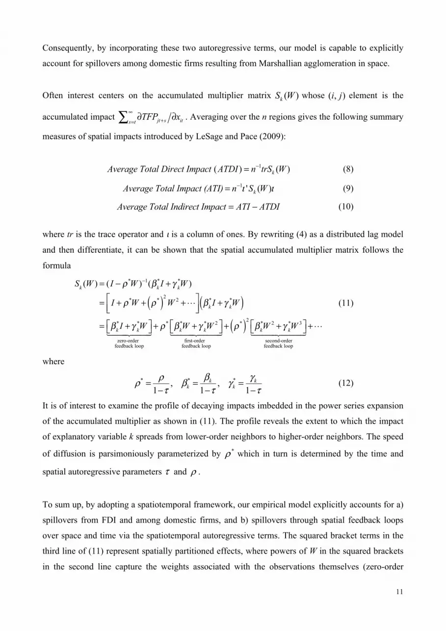
Consequently, by incorporating these two autoregressive terms, our model is capable to explicitly

account for spillovers among domestic firms resulting from Marshallian agglomeration in space.

Often interest centers on the accumulated multiplier matrix ( )kS W whose ( , )i j element is the

accumulated impact jt s its tTFP x∞

+=∂ ∂∑ . Averaging over the n regions gives the following summary

measures of spatial impacts introduced by LeSage and Pace (2009):

1( ) ( )kAverage Total Direct Impact ATDI n trS W−= (8)

1 ' ( )kAverage Total Impact (ATI) n S Wι ι−= (9)

Average Total Indirect Impact ATI ATDI= − (10)

where tr is the trace operator and ι is a column of ones. By rewriting (4) as a distributed lag model

and then differentiate, it can be shown that the spatial accumulated multiplier matrix follows the

formula

Sk (W ) = (I − ρ*W )−1(βk*I + γ k

*W )

= I + ρ*W + ρ*( )2W 2 +!⎡

⎣⎢⎤⎦⎥βk

*I + γ k*W( )

= βk*I + γ k

*W⎡⎣ ⎤⎦ zero-orderfeedback loop

" #$$$$$ %$$$$$+ ρ* βk

*W + γ k*W 2⎡⎣ ⎤⎦

first-orderfeedback loop

" #$$$$$$ %$$$$$$+ ρ*( )2

βk*W 2 + γ k

*W 3⎡⎣ ⎤⎦ second-orderfeedback loop

" #$$$$$$ %$$$$$$+!

(11)

where

* * *, ,1 1 1

k kk k

β γρρ β γτ τ τ

= = =− − −

(12)

It is of interest to examine the profile of decaying impacts imbedded in the power series expansion

of the accumulated multiplier as shown in (11). The profile reveals the extent to which the impact

of explanatory variable k spreads from lower-order neighbors to higher-order neighbors. The speed

of diffusion is parsimoniously parameterized by *ρ which in turn is determined by the time and

spatial autoregressive parameters τ and ρ .

To sum up, by adopting a spatiotemporal framework, our empirical model explicitly accounts for a)

spillovers from FDI and among domestic firms, and b) spillovers through spatial feedback loops

over space and time via the spatiotemporal autoregressive terms. The squared bracket terms in the

third line of (11) represent spatially partitioned effects, where powers of W in the squared brackets

in the second line capture the weights associated with the observations themselves (zero-order

 

12

impacts with 0W ), immediate neighbors (first-order impacts with 1W ), neighbors of neighbors

(second-order impacts with 2W ), and so on. These spatially partitioned summary measures are the

result of complex FDI spillovers being disentangled into narrow and wide geographic scopes, which

in turn can be used to identify and quantify spillovers from different channels. It is also due to these

complications, the focus of this paper will be on how to generate and interpret these spatially

partitioned effects base on the estimated model. To be more specific, equation (4) is estimated to

obtain consistent parameter estimates as an initial step. We then apply simulation-oriented Bayesian

approach to generate posterior distribution of the objects of interest. More details are described in

the following section.

4. Estimation Issues and Empirical Results

4.1 Estimation Issues

As the first step of our estimation analysis, System-GMM estimator is employed to obtain

consistent estimates of the parameters in Equation (4). Recent Monte-Carlo studies document that,

in the context of dynamic spatial panel model, system-GMM estimator performs well in terms of

bias, root mean squared error, and standard error accuracy. Kukenova and Monteiro (2009) perform

Monte-Carlo investigation and compare the performance of system-GMM with various other spatial

dynamic panel estimators.8 In the scenario that accounts for endogeneity problem, their results are

in favor of the system-GMM estimator. Jacobs et al. (2009) also perform a Monte-Carlo study on

the same topic but their research allows for the presence of both spatial lag and spatial error in the

model. Estimators proposed by Kelejian and Robinson (1993) and Kapoor, Kelejian and Prucha

(2007) are also invited for the performance comparison. Results of Jacobs et al. (2009) confirm the

findings of Kukenova and Monteiro (2009), i.e., system-GMM out performs other estimators.

Moreover, their Monte-Carlo evidence indicates that when system-GMM is adopted, differences in

bias, as well as root mean squared error, between spatial GMM estimates and corresponding GMM

estimates that ignore spatial correlation in error term are small. This research also documents that

the combination of collapsing the instrument matrix and limiting the lag depth of the dynamic

instruments substantially reduces the bias in estimating the spatial lag parameter, but hardly affects

its root mean squared error. In view of these recent developments in econometric literature, all point

estimates reported in this section are estimated by using the spatial system-GMM estimator. The

setup of moment conditions follows Kelejian and Prucha (1999), i.e., both space-time lagged

                                                                                                               8 These estimators include spatial MLE, spatial dynamic MLE (Elhorst, 2005), spatial dynamic QMLE (Yu et al., 2008),

LSDV, difference-GMM (Arellano and Bond, 1991), and system-GMM (Arellano and Bover, 1995; Blundell and Bond, 1998).

 

13

dependent variable and space lagged independent variables are included in the instrument list on top

of conventional instrument set for system-GMM suggested by (Arellano and Bover, 1995; Blundell

and Bond, 1998).

4.2 Empirical Results

Table 2 reports system-GMM estimation results of the spatiotemporal autoregressive panel model

in (4) and a conventional dynamic panel model without spatial interaction effects, i.e., no ρ and γ s

in (4). Both time and spatial autocorrelation coefficients are positive and significant, suggesting

fairly strong time and spatial self-reinforcing effects of total factor productivity for domestic private

firms at county level, suggesting significant spillovers among local firms resulting from Marshallian

agglomeration in space and over time. Estimated coefficients for own-regional (intra-regional) FDI

presence are in most cases negative and significant, indicating negative immediate impact from FDI

to domestic firms located in the same county. Note that, however, these two benchmark regressions

should be interpreted differently. For the spatiotemporal model, the partial derivative of TFP with

respect to a change in FDI presence not only measures the direct impact (as captured by 2β and 3β

in (4)) of this change on the own region but also measures its indirect impact (as captured by 2γ and

3γ in (4), the result of the feedback loop from the own region to neighboring regions and then back

to the own region). Consequently, the difference in the magnitude of coefficients is due to the fact

that conventional regression without spatial interactions is unable to capture these feedback effects

and thus provides potentially biased estimates.

The presence of SOEs, as captured by β1 and γ 1 , seems to generate negative impacts on domestic

firms. This is consistent with the results documented in the literature. SOEs tend to generate

crowding out effect as well as distortions in both input and output market. Note that the inter-

regional impact of SOEs presence, as captured by γ 1 , is small in magnitude and not significant.

This could be due to the fact that SOEs in China tend to focus on local regional markets for well-

documented cellular structure and localism; consequently, private firms are less affected by SOEs

from neighboring regions.

[Insert Table 2 here]

In what follows we describe how spatial direct and indirect impacts, as well as a set of partitioning

summary measures, can be generated from the estimated spatiotemporal model and how they can be

 

14

used to describe the extent of FDI spillovers over space and time. To account for spatial feedback

effects and draw inference from long-term equilibrium perspective, we report summary measures of

direct, indirect and total impacts as well as spatial partitioning of these impacts. To draw reliable

statistical inference from the sampling theory perspective on these impacts is not a straightforward

task as they are complicated, non-smooth functions of underlying model parameters as stated in (11)

and (12). On the other hand, a simulation-oriented Bayesian approach would have been relatively

straightforward if the posterior distribution of the underlying parameters were easy to sample from.

We apply the asymptotic theory in Kwan (1999) to interpret the asymptotic normal distribution of

the GMM estimator as an approximate posterior distribution, which in turn allows us to use

simulation method to compute the posterior distribution of various impact measures and their

spatial partitioning. More specifically, a random draw from the approximate posterior distribution

of the parameter vector ( , , , )θ τ ρ β γ= is ˆd Pθ δ θ= + , where θ is the value of the GMM estimate;

P is the lower-triangular Cholesky decomposition of the asymptotic covariance matrix of the GMM

estimator; and δ is a vector containing random draws from a standard normal distribution. Each

draw will result in one parameter combination for calculating impacts based on equations (8), (9)

and (10). Based on 5000 random draws, we can then compute very accurate estimate of the

moments and percentiles of the posterior distribution of the impacts.

Table 3 reports the marginal posterior distributions of direct, indirect and total impacts for the two

proxies of FDI penetration. Both posterior means of direct impact for FDI employment share and

sales income share are negative, suggesting FDI presence in a specific county is likely to generate

negative impacts on domestic private firms in the same county through taking over market share

and better employees from local firms. Nevertheless, the negative impact from market stealing may

pass through neighboring counties, as suggested by the negative indirect spillovers captured by FDI

sales income share. The knowledge spillovers through labor turnover, on the other hand, generate

positive and significant inter-regional spillovers. The inter-regional spillovers outweigh the intra-

regional spillovers in magnitude, resulting in positive average total FDI spillovers through labor

market in the long-term.

More precisely, assume that FDI employment share in all counties increases by 10% of the sample

mean (i.e., 0.111×10% = 0.011, see summary statistics in Appendix D), domestic private firms’

TFP on average would decrease by 0.844% (-0.768×0.011×100) due to direct impact from this

increase in FDI presence in the exact same county they are located. Domestic private firms’ TFP on

average would increase by 27.917% (25.379×0.011×100) due to indirect spillovers from the

increase in FDI presence in their neighboring counties, after accounting for impacts from spatial

 

15

feedback loops. Indirect spillovers outweigh the direct spillovers, leading to an overall increase of

27.072% (24.611×0.011×100) in TFP. On the other hand, if FDI sales income share in all counties

increases by 10% of the sample mean (i.e., 0.127×10% = 0.013), the associated direct spillovers

among to a 4.445% decrease in TFP and an even larger decrease of 53.468% due to indirect

spillovers. The total spillovers in this case amount to 57.912% decrease in TFP of domestic private

firms.

[Insert Table 3 here]

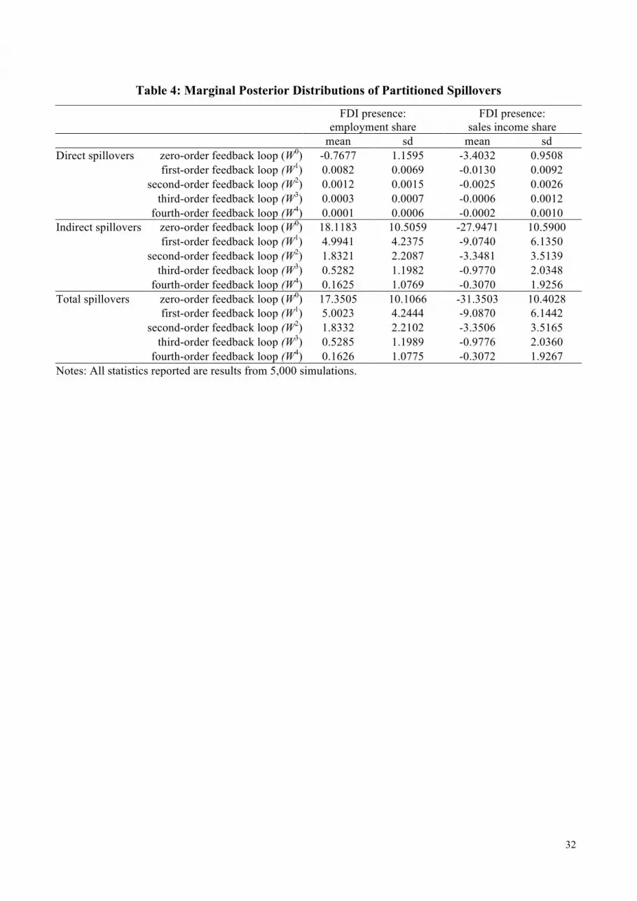
Table 4 reports statistics for spatially partitioned impacts based on 5,000 simulations. As discussed

in previous section, these summary partitioned measures not only describe the decay pattern of

spillovers but also decompose them into narrow and wide geographic scopes. The results indicate

that, for both of the two FDI proxies we adopted in this study, the intra-regional (direct) spillovers

and inter-regional (indirect) spillovers present very different spatial decay pattern. On average, the

intra-regional spillovers become almost negligible even in first-order feedback loop (impact from

immediate neighbors with W 1 being the weight). Notice that the magnitudes of first-order feedback

in both cases are very small, implying that the penetration of FDI in a specific county on average

will affect its immediate neighbors, which in return will generate some but almost negligible

feedback impacts to the domestic private firms in this specific county. The magnitudes of inter-

regional spillovers, however, are still quantitatively significant in the third-order feedback loop and

could even extend to the fourth-order feedback loop. These results suggest that, among spatial

feedback loops, the negative intra-regional FDI spillovers decay very fast and are almost bounded

locally while the inter-regional FDI spillovers present slower decay pattern and could extend to

higher order neighbors.

As spatially partitioned impacts decompose impacts into narrow and wide geographic scopes, the

results in Table 4 also filter and identify spillovers that pass through these scopes and reach

domestic firms in different manners. As discussed in previous section, spillovers through labor

turnover channel could be both negative (poaching local talents) and positive (knowledge spillover)

that are operative at the same time. Knowledge spillovers, nevertheless, should have wider

geographic scope than poaching effect. The results in Table 4 seem to have disentangled these two

impacts successfully. The negative impacts in narrow scope (direct spillovers) are due to poaching

whereas the positive knowledge spillovers become dominant in wider scope (indirect spillovers).

Negative market stealing effect as captured by sales income share is negative in both narrow and

wide scopes, which is consistent with our conjecture that such spillover has no boundary in a

 

16

rapidly integrated market.

[Insert Table 4 here]

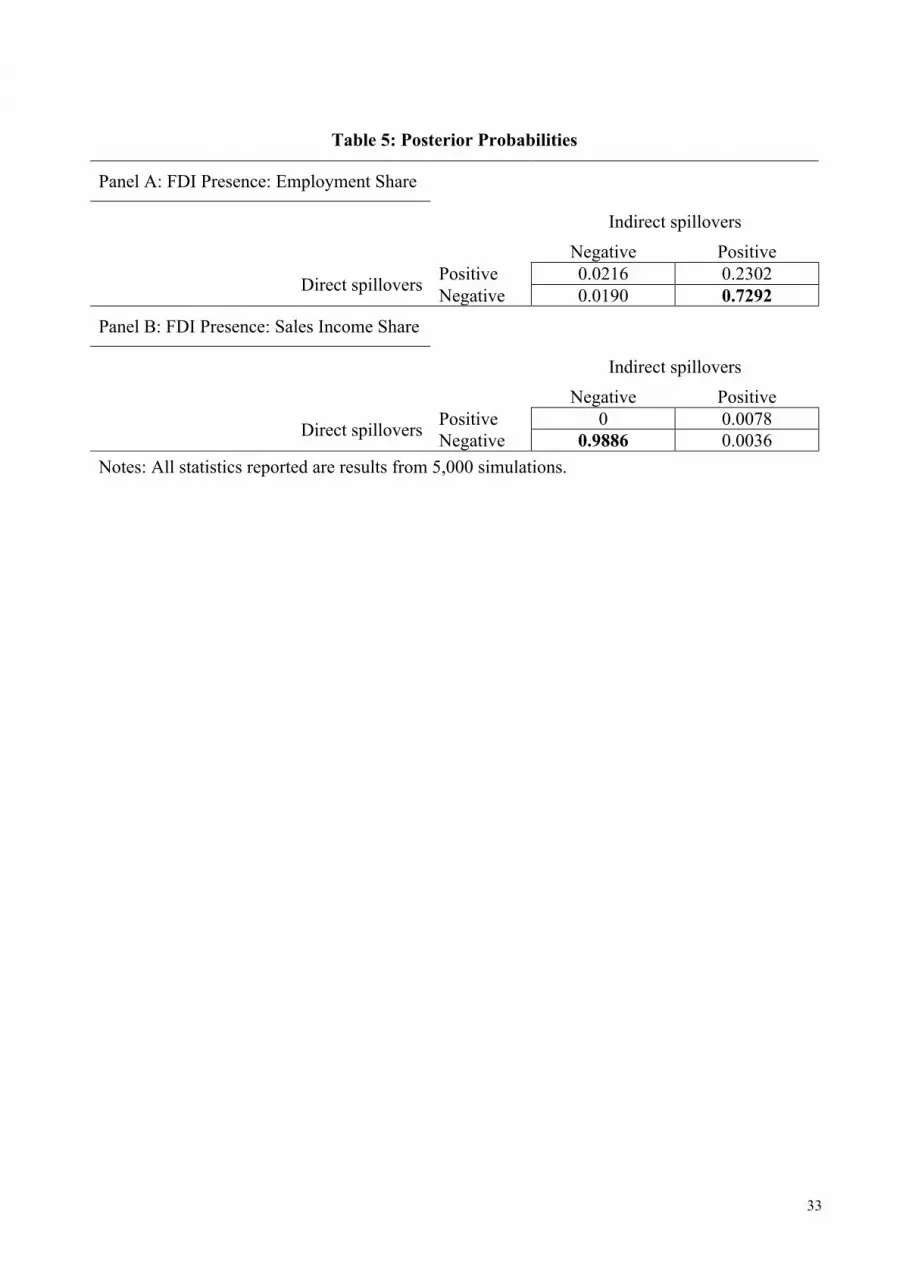
In Table 5, we present the posterior probabilities of spillovers for both FDI employment share and

FDI sales income share based on simulated data. This table describes the most likely outcome when

various spillover channels operate at the same time. In each 2 by 2 table, based on 5,000

simulations, we calculate the probabilities of positive or negative spillovers for both direct and

indirect impacts. The statistics reveal that the probabilities are not evenly distributed in all four

scenarios. As for FDI employment share (Panel A), the probability for positive indirect and

negative direct impacts is the highest (0.7292). This suggests that, through poaching or cherry

picking local employees, MNEs generate locally bounded negative effect on the productivity

performance of domestic firms located in the same county. Domestic firms located in neighboring

counties, on the other hand, are likely to benefit from FDI knowledge spillovers which diffuse

beyond borders. As for FDI sales income share (Panel B), the probability for both negative direct

and indirect impacts outcome is the highest (0.9886) among all four scenarios, suggesting a

sweeping market stealing effect that adversely affects domestic firms irrespective of geographical

distance.

Figure 4 depicts density-distribution sunflower plots following Dupont and Plummer (2003).9 With

the aid of these plots we are able to display density of bivariate data (direct and indirect impacts) in

a two dimensional graph. As presented in the figure, for FDI employment share, high- and medium-

density regions are mainly located in the quadrant of negative direct spillovers and positive indirect

spillovers. For FDI sales income share, high- and medium-density regions are mainly located in the

quadrant where both direct and indirect spillovers are negative. These results are consistent with the

posterior probabilities presented in Table 5. An additional interesting finding is that, as shown by

the fitted line, for both FDI employment share and sales income share, direct and indirect spillovers

are significantly and negatively correlated; with slope coefficients are -0.0165 and -0.0080

respectively. These negative correlations, as well as the fact that the one for FDI employment share

is much stronger (more than double compared to FDI sales income share), remain puzzling to us

and warrant further investigation in future research.

                                                                                                               9 These sunflower plots are obtained with the aid of Stata (version 11.2) function ‘sunflower’. In sunflower plots, a

sunflower is presented as several line segments with equal length, called petals. These petals radiate from a central point. There are two varieties of sunflowers, namely light sunflower and dark sunflower. Each petal of a light sunflower represents 1 observation and each petal of a dark sunflower represents several observations. Dark and light sunflowers represent high- and medium-density regions of the data, and marker symbols represent individual observations in low-density regions.

 

17

[Insert Table 5 and Figure 4 here]

5. Conclusions and Policy Implications

The diffusion and materialization of FDI spillovers are neither automatic nor universal; instead,

they are affected by various simultanuously operating factors drawn from both economic and

geographical dimensions. These factors are of different geographic scopes and reach domestic firms

in different manners. How to identify and then quantify these resulting impacts separately remain a

challenging yet important issue in the literature. We investigate in this paper the geographic extent

of various FDI spillover channels and their diffusion pattern by means of a large panel data set of

Chinese manufacturing firms and their location information down to county level. In particular,

geographical distance is used to disentangle spillovers with different scopes from a complex overall

effect. Working with a spatiotemporal panel regression model, we are able to identify and uncover

the sign, the magnitude, and the geographic attenuation pattern of FDI spillover effects from

different channels.

We find that intra-regional spillovers tend to be negative, irrespective of spillover channels. Inter-

regional spillovers, on the other hand, could be negative or positive depending on spillover

channels. These findings are consistent with common belief about the sign and scope of FDI

spillovers. Given that it is relatively costly to poaching local talents from distant domestic firms

whereas barries and communication cost for knowledge spillovers have been significantly reducing,

our method identifies negative poaching impact in narrow scope and positive knowledge spillovers

in wide scope. Our result also documents that negative market stealing effect does not have

boundary and could extend from narrow scope to wide scope via rapidly integrated market.

What is the policy take-away of this paper? In order to attract FDI and, most importantly, to

facilitate domestic firms to learn from nearby foreign firms with advanced technology, China’s

government has been providing incentive package for MNCs, as well as adopting place-based

policy since the early 1990s. Corresponding strategies include tax holiday or reduction, job-creation

subsidies, preferential loan to FDI, special economic zones and similar schemes, and construction

of industrial facilities (land and infrastructure are subsidized) provided by both central and local

governments. Many local governments also compete with their neighboring governments in this

regard, which partially results in severe strategic tax competition and ‘race to the top / race to the

bottom’ problem (Yao and Zhang, 2008). One major findings of this paper is that domestic firms

 

18

mainly benefit from FDI presence in their neighboring regions, whereas FDI direct impacts to a

specific location itself are likely to be negative. Consequently, as far as a particular local

government is of concern, it is important to rethink about the strategic tax competition approach for

attracting FDI, as the benefit from doing so may not be as large as commonly believed. A better

strategy for local governments is to cooperate with each other to provide better environment for

both MNCs and domestic firms, such as providing better infrastructure for transportation across

regions, lower regional tariff for capital and labor, and fair tax treatment for both MNCs and

domestic firms. To this end, coordination between local governments would be of utmost

importance.

  19

Appendix A: Ownership Structure and Their Corresponding Portions in NBS-CIE Database

Domestic Firms Foreign Firms Sino-Foreign Joint Ventures (JVs) Others

Privates SOEs

(1) (2) (3) (4) (5) (6) (7) (8): sum of (1) to

(7) (9) (10)

(11): (9) + (10)

(12) (13) (14)

(15): (12) + (13) + (14)

(16) (17) (18)

(19): (16) + (17) + (18)

(20)

Year No. of Firms Pure

Privates

Other Domestic

Private Firms

Collective Enterprise

Joint-Stock

Enterprise

Associated Economics

Limited Liability Company

Corporation Limited

Enterprises

All Domestic Privates

Pure SOEs

SOEs-Domestic

JVs SOEs

Pure F-type

FDI

Pure HMT-

type FDI

Joint Ventures between

F and HMT

FDI Sino-

Foreign JVs

Sino-HMT JVs

Other Sino-

Foreign JVs

Sino-Foreign

JVs Undefined

Total: (8) + (11) + (15) + (19) + (20)

1998 102830 11.25 3.36 30.44 4.44 1.54 2.49 1.18 54.70 16.48 5.87 22.35 2.84 3.88 0.03 6.75 6.43 6.76 0.27 13.46 2.74 100 1999 111715 13.17 4.53 27.44 4.48 1.43 3.17 1.39 55.60 14.80 5.96 20.76 3.13 4.97 0.04 8.14 5.89 6.60 0.25 12.75 2.76 100 2000 110090 19.10 5.80 22.25 4.08 1.19 4.27 1.47 58.17 11.99 5.34 17.33 3.41 5.50 0.05 8.96 5.77 6.84 0.23 12.85 2.69 100 2001 125235 26.56 7.86 16.84 3.66 0.95 5.57 1.52 62.96 8.97 4.32 13.29 3.83 5.82 0.05 9.70 5.44 6.19 0.22 11.85 2.21 100 2002 136163 32.63 9.12 13.26 2.84 0.71 5.98 1.52 66.06 7.26 3.65 10.90 4.28 5.69 0.07 10.04 5.34 5.36 0.20 10.89 2.10 100 2003 153585 37.94 10.95 9.38 2.22 0.52 6.46 1.47 68.95 5.30 2.70 8.00 4.72 6.35 0.05 11.12 5.01 4.89 0.16 10.06 1.88 100 2004 219335 44.28 11.83 5.59 1.56 0.31 7.70 1.21 72.47 3.21 1.76 4.97 5.72 6.58 0.05 12.36 4.79 4.11 0.13 9.03 1.18 100 2005 218401 44.93 13.76 4.47 1.28 0.26 7.44 1.19 73.34 2.44 1.37 3.81 5.97 6.88 0.05 12.91 4.41 3.68 0.10 8.19 1.76 100 2006 239352 47.68 14.12 3.75 1.36 0.21 7.08 1.01 75.21 1.89 1.09 2.98 5.89 6.70 0.05 12.64 4.09 3.31 0.09 7.49 1.69 100 2007 266311 48.43 16.27 2.96 1.14 0.17 6.90 0.92 76.78 1.42 0.86 2.28 5.92 6.55 0.05 12.52 3.67 2.91 0.09 6.67 1.75 100

Notes: This table is produced based on total record of 503079 firms with 1683017 observations after we clearn up the dataset by following the suggestions provided in Brandt et al. (2012). All statistics reported are results after data cleaning. A firm’s ownership structure is determined by its source and structure of Paid in Capital and their registered type. ‘Pure’ means the Paid in Capital is 100% from the corresponding source; for instance, ‘Pure Private’ means all the Paid in Capital of these firms are from private sector. HMT denotes foreign firms from Hong Kong, Macau, and Taiwan. F denotes foreign firms from countries / regions other than Hong Kong, Macau, and Taiwan. Source: Authors’ calculation based on NBS-CIE database.

 

 

20

Appendix B: Data and Variable

In this paper we employ data from the annual census of above-size manufacturing firms

conducted by the National Bureau of Statistics (NBS) of China (known as the Chinese Industrial

Enterprises Database, NBS-CIE database henceforth) from 1998 to 2007. Our data cleaning process

follows closely the suggestions provided in Brandt et al. (2012 and 2014). For this study, we drop

firms with employment (personal engaged) below 8 workers and firms with negative nominal

capital stocks, paid-up capital, sales revenue, value added, or intermediate inputs. We use industry

concordances provided by Brandt et al. (2012) as consistent industry identifier throughout the

sample period. Nominal input and output data are deflated by input and output deflators at 2-digit

industry level (1998 = 100), which are also obtained from Brandt et al. (2012).

Variables for capital stock in the original NBS-CIE database could not serve as good measures

for capital input. Firms in the database do not report fixed investment. Fixed capital stock data are

reported as the sum of book values in different years’ price level, which cannot be used directly for

TFP estimation. We thus compute a real capital stock series using the perpetual inventory approach

proposed in Brandt et al. (2012 and 2014).

We first make use of the capital stock data reported in 1993 annual enterprise survey and in 1998

NBS-CIE database to estimate average growth rate of the nominal capital stock between 1993 and

1998 at province by industry (2-digit) level. By using this estimated growth rate ( g ), together with

capital stock at original purchase price ( initialfa ) and the firm’s age (age ), we calculate the firm’s

initial nominal capital stock ( 0nk ) in the establishment year, nk0 = fainitial (1+ g)age

.10 The firm’s

real capital stock in the establishment year ( rk0 ) is obtained by deflating 0nk using investment

deflator (1998 = 100) constructed by Perkins and Rawski (2008).11 Nominal capital stock data after

the establishment year is then calculated by using the estimated growth rate ( g ). Assuming a 9%

depreciation rate, the real capital stock data in 1998 (or the firm’s first year in the sample) is then

calculated by using perpetual inventory method and Perkins and Rawski deflators. Real capital

stock after 1998 (or after the firm’s first year in the sample) is calculated by following the same

perpetual inventory method with 9% depreciation rate but use the first difference in firm’s nominal

capital stock measured at original purchase prices as fixed investment for each year.

                                                                                                               10 Following Brandt et al. (2012 and 2014), we assume that, for firms with establishment year earlier than 1978, their

experience before 1978 have negligible impact on the capital stock in 1998 and thus reset the establishment year for these firms to 1978.

11 Deflators up to 2006 are reported in Brandt et al. (2012). We thank Yifan Zhang for confirming our calculation of deflator for 2007 by following the chain-link approach in Perkins and Rawski (2008).  

 

21

Appendix C: Constructing County-level TFP from Firm-level Data

County-level TFP in Eq. (4) is constructed as the weighted average of firm-level ln( )TFP s

with the weights being the value added shares of the firm in the underlying county in each year.

Specifically, itTFP , for county i , in year t is constructed as

ln( )jitit jit

jitj i

vaTFP TFP

va∈

=∑

where jitva denotes the year t ’s value added for firm j located in county i .

Our estimation procedure for firm-level productivity in logarithm, ln( )TFP , largely follows the

algorithm initiated by Olley and Pakes (1996) and then further developed by Levinsohn and Petrin

(2003) with the aim to tackle the potential endogeneity problem arising from potential correlation

between input levels and unobserved firm-specific productivity shocks. This algorithm is

commonly referred as “proxy variable approach” in the literature (Amit et al., 2008). We

nevertheless do go beyond this conventional approach to incorporate some new developments in the

literature, which are mainly drawn from Ackerberg et al. (2006), Melitz and Levinsohn (2006) and

De Loecker and Warzynski (2012). Given that Levinsohn and Petrin (2003) (LP hereafter)

algorithm has become a standard method in the literature and has been reintroduced in many studies,

in the following we should focus on discussing the places in our procedure that have departed from

conventional LP routine.12

The first departure from the conventional LP routine is in the functional form used for

production function. Instead of using Cobb-Douglas production function, we adopt a translog

production function that includes all the (logged) inputs and their second order polynomial terms,

i.e., (logged) inputs squared and interaction terms between all (logged) inputs. This departure

avoids the assumptions of 1) perfect substitution between production factors; 2) constant output

elasticity across firms and over time; and 3) perfect competition in the production factors market

across firms and over time, which are all too restrictive to be valid in the empirical application (De

Loecker and Warzynski, 2012). More specifically, in a specific industry, for a value added translog

production function we have

2 2jt l jt k jt ll jt kk jt lk jt jt jt jtva l k l k l k wβ β β β β ε= + + + + + +

                                                                                                               12 For more comprehensive discussion on both theoretical and empirical issues of this topic, the interested reader is

referred to Ackerberg et al. (2006), Melitz and Levinsohn (2006), Van Beveren (2012), and De Loecker and Warzynski (2012).

 

22

where jtva , jtl , jtk , and jtw are respectively firm j ’s value added, labor input, capital input, and

unobserved productivity component at time t . All variables are in logarithm. jtε is an error term

that is assumed to be uncorrelated with all input choices. Firms will make input decisions based on

their productivity; thus, productivity component jtw  is correlated to input choices. Since data for

jtw usually is not available; consequently, conventional method like OLS will lead to bias

estimation, unless a valid proxy for productivity could be included in the regression as control

variable.

To proxy for productivity, we follow Levinsohn and Petrin (2003) to rely on material demand

function, which assumes that demand for the intermediate input, mjt , is a monotonous (increasing)

function of wjt , i.e., ( , )jt t jt jtm m k w= , where both jtk and jtw are state variables based on which

firms make their input decisions. The productivity component, jtw , is then constructed by inverting

this demand function to get ( , )jt t jt jtw h m k= .13

As the second departure from the conventional LP method, we explore and include additional

state variables and other demand conditions in (.)th . This departure follows Melitz and Levinsohn

(2006) and De Loecker and Warzynski (2012) with an aim to incorporate more variables that

potentially affect firms’ optimal input demand choice. Failing to do so would weaken the validity of

using intermediate inputs as a proxy for productivity. Consequently, we include in (.)th a vector

jtz , i.e., ( , , )jt t jt jt jtw h m k z= , where jtz includes a dummy for export status (equals 1 if export

value is positive), a dummy for R&D status (equals 1 if R&D expenditure is positive), a survival

propensity score described in Olley and Pakes (1996), and a demand condition derived in Melitz

and Levinsohn (2006) to allow for product heterogeneity and imperfect competition.14

The final departure from LP routine is that, instead of identifying labor coefficient in a first stage,

we identify all the coefficients at once and in the final stage. Ackerberg et al. (2006) illustrate that

                                                                                                               13 Included in (.)th are 2 2, , , and jt jt jt jt jt jtm m k m k m . 14 NBS-CIE database, like many other firm level datasets, does not report either physical output or physical attributes

for this output. A common solution is to use industry-level input and output deflators to deflate nominal terms. If firms in an industry produce homogeneous goods, an assumption that is implicitly assumed in the conventional LP routine, the above approach could yield a valid proxy for the unobserved physical output. However, since firms are likely to produce goods that are differentiated, firm level prices will fluctuate relative to the industry price index and hence break the link between deflated sales and physical output. Both Van Beveren (2012) and De Loecker and Warzynski (2012) illustrate the potential bias in the process of production function estimation, and thus in productivity, if this problem is not addressed appropriately. Under some modest assumptions, Melitz and Levinsohn (2006) show that including a demand condition, [(rt − !pt )− nt ] (where, everything in logarithm, rt − !pt ,   is total

industry deflated sales and tn is the number of firms in the industry) in a conventional deflated production function is sufficient enough to eliminate the impact of unobserved firm level prices.  

 

23

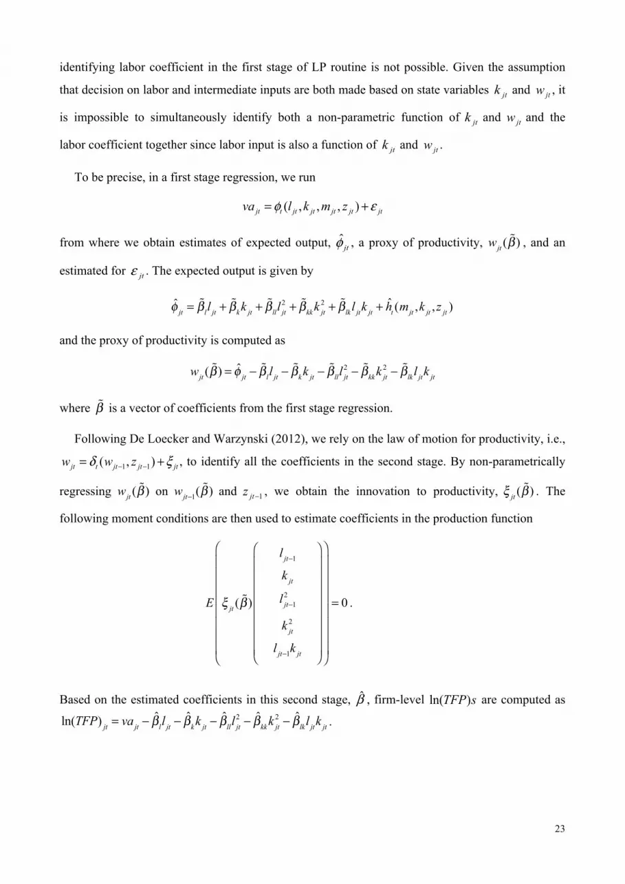
identifying labor coefficient in the first stage of LP routine is not possible. Given the assumption

that decision on labor and intermediate inputs are both made based on state variables jtk and jtw , it

is impossible to simultaneously identify both a non-parametric function of jtk and jtw and the

labor coefficient together since labor input is also a function of jtk and jtw .

To be precise, in a first stage regression, we run

( , , , )jt t jt jt jt jt jtva l k m zφ ε= +

from where we obtain estimates of expected output, ˆjtφ , a proxy of productivity, wjt ( !β ) , and an

estimated for jtε . The expected output is given by

φ jt =

!βll jt +!βkk jt +

!βlll jt2 + !βkkk jt

2 + !βlk l jtk jt + ht (mjt ,k jt , z jt )

and the proxy of productivity is computed as

wjt ( !β ) = φ jt −

!βll jt −!βkk jt −

!βlll jt2 − !βkkk jt

2 − !βlk l jtk jt

where !β is a vector of coefficients from the first stage regression.

Following De Loecker and Warzynski (2012), we rely on the law of motion for productivity, i.e.,

1 1( , )jt t jt jt jtw w zδ ξ− −= + , to identify all the coefficients in the second stage. By non-parametrically

regressing wjt ( !β ) on

wjt−1( !β ) and 1jtz − , we obtain the innovation to productivity,

ξ jt ( !β ) . The

following moment conditions are then used to estimate coefficients in the production function

E ξ jt ( !β )

l jt−1

k jt

l jt−12

k jt2

l jt−1k jt

⎛

⎝

⎜⎜⎜⎜⎜⎜⎜⎜

⎞

⎠

⎟⎟⎟⎟⎟⎟⎟⎟

⎛

⎝

⎜⎜⎜⎜⎜⎜⎜⎜

⎞

⎠

⎟⎟⎟⎟⎟⎟⎟⎟

= 0 .

Based on the estimated coefficients in this second stage, β , firm-level ln( )TFP s are computed as

ln(TFP) jt = va jt − βll jt − βkk jt − βlll jt

2 − βkkk jt2 − βlk l jtk jt .

  24

Appendix D: Summary Statistics at County Level

Percentile

Mean Standard Deviation 5% 25% 50% 75% 95% Obs.

TFP of Domestic Private Firms 2.6384 2.3566 0.1994 1.1455 2.2469 3.6115 6.3601 17187 FDI Presence: Employment Share 0.1112 0.1727 0 0 0.0320 0.1530 0.4968 18167 FDI Presence: Sales Income Share 0.1270 0.1987 0 0 0.0298 0.1726 0.5898 18167 SOEs Presence 0.3467 0.3300 0 0.0380 0.2464 0.6127 0.9876 18165 W * TFP of Domestic Private Firms 1.4648 0.6266 0.5139 0.9587 1.4327 1.9491 2.5028 18167 Space-time lagged TFP of Domestic Private Firms 1.3452 0.5966 0.4645 0.8608 1.2937 1.8077 2.3388 15519 W * FDI Presence: Employment Share 0.0664 0.0281 0.0229 0.0446 0.0650 0.0862 0.1133 18167 W * FDI Presence: Sales Income Share 0.0757 0.0299 0.0272 0.0531 0.0755 0.0997 0.1209 18167 W * SOEs Presence 0.1941 0.1010 0.0647 0.1129 0.1626 0.2699 0.3819 18165 Source: Authors’ calculation based on NBS-CIE database.

 

 

25

Figure 1: FDI Spatial Density Distribution at County Level

FDI Density (Fixed Asset Share) at County Level (1998)

FDI Density (Fixed Asset Share) at County Level (2007)

Source: Authors’ calculation based on NBS-CIE database. FDI density is measured by fixed asset share of FDI in each county, i.e., the value of fixed asset of foreign firms divided by the total fixed asset in a county. The color code on the map indicates the classes of density in quartiles, with the darkest color corresponding to the class of the highest density.

  26

Figure 2: Moran Scatterplot of County-Level TFP in 1998, 2003, and 2007

Notes: County level TFPs are constructed as the weighted average of firm-level ln(TFP)s with the weight being the value added share of each firm in the underlying county. All statistics are calculated based on row-standardized spatial weights matrix with 10 nearest neighbors. Source: Authors’ calculation based on NBS-CIE database.

 

-1-.5

0.5

1

Spat

ially

lagg

ed T

FP fo

r dom

estic

priv

ate

firm

s in

199

8, s

tand

ardi

sed

-1 0 1 2 3 4TFP for domestic private firms in 1998, standardised

Moran Scatterplot of Spatially Lagged TFPagainst TFP in 1998: Domestic Private Firms

Moran's I = .045 (p-value = < 0.001)

-1-.5

0.5

1

Spat

ially

lagg

ed T

FP fo

r dom

estic

priv

ate

firm

s in

200

3, s

tand

ardi

sed

-1 0 1 2 3TFP for domestic private firms in 2003, standardised

Moran Scatterplot of Spatially Lagged TFPagainst TFP in 2003: Domestic Private Firms

Moran's I = .082 (p-value = < 0.001)

-1-.5

0.5

1

Spat

ially

lagg

ed T

FP fo

r dom

estic

priv

ate

firm

s in

200

7, s

tand

ardi

sed

-2 -1 0 1 2 3TFP in 2007, standardised

Moran Scatterplot of Spatially Lagged TFPagainst TFP in 2007: Domestic Private Firms

Moran's I = .148 (p-value = < 0.001)

 

27

Figure 3: Local Indicator of Spatial Association (LISA) Cluster Map of Domestic Private Firms

Note: LISA = Local Indicator of Spatial Association. Source: Authors’ calculation based on NBS-CIE database.

 

28

Figure 4: Joint Posterior Distribution of Direct/Indirect Cumulative Spillovers

Source: Authors’ calculation based on simulated data.

 

29

Table 1: Global Moran’s I for County-Level TFP of Domestic Private Firms

Moran’s I Standard Deviation p-value

10 nearest neighbors TFP in 1998 0.0451 0.0106 < 0.001 TFP in 2003 0.0817 0.0097 < 0.001 TFP in 2007 0.1477 0.0102 < 0.001

5 nearest neighbors

TFP in 1998 0.0582 0.0141 < 0.001 TFP in 2003 0.0910 0.0120 < 0.001 TFP in 2007 0.1557 0.0122 < 0.001

Notes: All statistics are calculated based on row-standardized spatial weights matrix with 5 or 10 nearest neighbors have non-zero spatial weight wij. County level TFPs are constructed as the weighted average of firm-level ln(TFP)s with the weight being the value added share of each firm in the underlying county. Source: Authors’ calculation based on NBS-CIE database.

 

30

Table 2: Benchmark Regression

Dependent variable: TFP No spatial effects Spatiotemporal model

Time lagged TFP 0.259 0.307 (0.046) (0.044) SOE presence -3.667 -3.704 (0.482) (0.511) FDI presence: employment share -1.459 -0.540 (0.675) (0.811) FDI presence: sales income share -1.468 -2.353 (0.672) (0.650) Space-time lagged TFP 0.305 (0.152) Spatially lagged SOE presence -0.677 (1.354) Spatially lagged FDI presence: employment share 21.006 (12.311) Spatially lagged FDI presence: sales income share -32.423 (12.464) Hansen Statistic 3.433 11.121 Hansen Statistic P-value 0.842 0.744 D.O.F of Hansen Statistic 7 15 Number of Instruments 20 32 N 14560 14560 Notes: Results reported are two-step system-GMM estimates. Standard errors in parentheses. Windmeijer’s (2005) correction method for the two-step standard errors is employed. Year dummies are included in all regressions. Collapsed instrument matrix technique is employed to reduce the instrument count.

 

31

Table 3: Marginal Posterior Distributions of Cumulative Spillovers

Percentile mean sd 5% 25% 50% 75% 95% FDI: employment share

Direct spillovers -0.768 1.153 -2.649 -1.562 -0.774 -0.021 1.144 Indirect spillovers 25.379 15.875 1.300 14.596 24.362 34.747 52.458

Total spillovers 24.611 15.648 1.089 13.841 23.601 33.796 51.268 FDI: sales income share

Direct spillovers -3.419 0.949 -4.982 -4.063 -3.432 -2.783 -1.849 Indirect spillovers -41.129 18.909 -75.784 -51.474 -39.426 -27.895 -14.556

Total spillovers -44.548 18.773 -78.448 -54.815 -42.654 -31.242 -18.124 Notes: All statistics reported are results from 5,000 simulations.

 

32

Table 4: Marginal Posterior Distributions of Partitioned Spillovers

FDI presence: employment share

FDI presence: sales income share

mean sd mean sd Direct spillovers zero-order feedback loop (W0) -0.7677 1.1595 -3.4032 0.9508 first-order feedback loop (W1) 0.0082 0.0069 -0.0130 0.0092 second-order feedback loop (W2) 0.0012 0.0015 -0.0025 0.0026 third-order feedback loop (W3) 0.0003 0.0007 -0.0006 0.0012 fourth-order feedback loop (W4) 0.0001 0.0006 -0.0002 0.0010 Indirect spillovers zero-order feedback loop (W0) 18.1183 10.5059 -27.9471 10.5900 first-order feedback loop (W1) 4.9941 4.2375 -9.0740 6.1350 second-order feedback loop (W2) 1.8321 2.2087 -3.3481 3.5139 third-order feedback loop (W3) 0.5282 1.1982 -0.9770 2.0348 fourth-order feedback loop (W4) 0.1625 1.0769 -0.3070 1.9256 Total spillovers zero-order feedback loop (W0) 17.3505 10.1066 -31.3503 10.4028 first-order feedback loop (W1) 5.0023 4.2444 -9.0870 6.1442 second-order feedback loop (W2) 1.8332 2.2102 -3.3506 3.5165 third-order feedback loop (W3) 0.5285 1.1989 -0.9776 2.0360 fourth-order feedback loop (W4) 0.1626 1.0775 -0.3072 1.9267 Notes: All statistics reported are results from 5,000 simulations.

 

33

Table 5: Posterior Probabilities

Panel A: FDI Presence: Employment Share

Indirect spillovers Negative Positive

Direct spillovers Positive 0.0216 0.2302 Negative 0.0190 0.7292

Panel B: FDI Presence: Sales Income Share

Indirect spillovers Negative Positive

Direct spillovers Positive 0 0.0078 Negative 0.9886 0.0036

Notes: All statistics reported are results from 5,000 simulations.

34  

References

Abraham, F., Konings, J., & Slootmaekers, V., (2010). FDI spillovers in the Chinese manufacturing sector. Economics of Transition, 18, 143-182.

Abreu, M., De Groot, H. L. F., & Florax, R. J. G. M., (2005). Space and growth: A survey of empirical evidence and methods. Région et Développement, 21, 13-43.

Ackerberg, D. A., Kevin, C., & Garth F., (2006). Structural Identification of Production Functions, Unpublished Manuscript, UCLA Economics Department.

Aitken, B. J., & Harrison, A. E., (1999). Do domestic firms benefit from direct foreign investment? Evidence from Venezuela. American Economic Review, 89, 605-618.

Amit, G., Salvador, N., & David, R., (2008). Estimating Production Functions with Heterogeneous Firms. 2008 Meeting Papers 935, Society for Economic Dynamics.

Anselin, L., (1995). Local indicators of spatial association – LISA. Geographical Analysis, 27, 93–115.

Anselin, L., (2001). Spatial econometrics, in Baltagi B. (ed.) A Companion to Theoretical Econometrics, Blackwell, Oxford, 310–330.

Arellano, M., & Bond, S., (1991). Some tests of specification for panel data: Monte-Carlo evidence and an Application to employment equations. Review of Economic Studies, 58, 277-297.

Arellano, M., & Bover, O., (1995). Another look at the instrumental variable estimation of error-components models. Journal of Econometrics, 68, 29-51.

Audretsch, D. B., & Feldman, M., (1996). Spillovers and the geography of innovation and production. American Economic Review, 86, 630–640.

Blalock, G., & Gertler, P. J., (2008). Welfare gains from Foreign Direct Investment through technology transfer to local suppliers. Journal of International Economics, 74, 402-421.

Blonigen, B. A., Ellis, C. J., & Fausten, D., (2005). Industrial groupings and foreign direct investment. Journal of International Economics, 65, 75-91.

Blundell, R., & Bond, S., (1998). Initial conditions and moment restrictions in dynamic panel data models. Journal of Econometrics, 87, 115-143.

Boschma, R. A., & Frenken, K., (2010). The spatial evolution of innovation networks. A proximity perspective. In R. A. Boschma, R. Martin (eds), The Handbook of Evolutionary Economic Geography, pp. 120–135. Cheltenham: Edward Elgar.

Brandt, L., Van Biesebroeck, J., & Zhang, Y. F., (2012). Creative Accounting or Creative Destruction? Firm-level Productivity Growth in Chinese Manufacturing. Journal of Development Economics 97, 339-351.

Brandt, L., Van Biesebroeck, J., & Zhang, Y. F., (2014) Challenges of Working with the Chinese NBS Firm-Level Data, China Economic Review, 30, 339-352.

35  

Cheng, L. K., (1994). Foreign direct investment in China, Organisation for Economic Co-operation and Development, Report COM/DAFFE/IME/TD (94) 129, November 1994.

Cheng, L. K., & Kwan, Y. K., (2000a). What are the determinants of the location of foreign direct investment? The Chinese experience. Journal of International Economics, 51, 379-400.

Cheng, L. K., & Kwan, Y. K., (2000b). The location of foreign direct investment in Chinese regions: further analysis of labor quality. In: Ito T. and Krueger A.O. (Eds.), The Role of Foreign Direct Investment in East Asian Economic Development. Chicago, IL: University of Chicago Press.

Ciccone, A., & Hall, R. E., (1996). Productivity and the density of economic activity. American Economic Review, 86, 54-70.

Damijan, J. P., Rojec, M., Majcen, B., & Knell, M., (2013). Impact of Firm Heterogeneity on Direct and Spillover Effects of FDI: Micro-evidence from Ten Transition Countries, Journal of Comparative Economics, 41 (3), 895-922.

De Loecker, J., & Warzynski F., (2012). Markups and firm-Level export status. American Economic Review, vol. 102 (6), pages 2437-71, October.

Dupont, W. D., & Plummer, Jr. W. D., (2003). Density distribution sunflower plots. Journal of Statistical Software, 8: 1-11.

Duranton, G., & Puga, D., (2004). Micro-foundations of urban agglomeration economies. In J. V. Henderson, J. F. Thisse (eds) Handbook of Regional and Urban Economics, vol. 4, Chapter 48, pp. 2063–2117. Amsterdam: Elsevier/North-Holland.

Elhorst, J. P., (2005). Unconditional maximum likelihood estimation of linear and log-linear Dynamic models for spatial panels. Geographical Analysis, 37, 85-106.

Ellison, G., Glaeser, E., & Kerr, W., (2010). What causes industry agglomeration? Evidence from coagglomeration patterns. American Economic Review, 100, 1195–1213.

Fallick, B., Fleischman, C., & Rebitzer, J., (2006). Job-hopping in Silicon Valley: some evidence concerning the microfoundations of a high-technology cluster. Review of Economics and Statistics, 88, 472–481.

Freedman, M., (2008). Job hopping, earnings dynamics, and industrial agglomeration in the software publishing industry. Journal of Urban Economics, 64, 590–600.

Gertler, M. S., (2003). Tacit knowledge and the economic geography of context or the undefinable tacitness of being (there). Journal of Economic Geography, 3, 75–99.

Hale, G., & Long, C., (2011). Are there productivity spillovers from foreign direct investment In China? Pacific Economic Review, 16, 135-153.

Head, K., Ries, J., & Swenson, D., (1995). Agglomeration benefits and location choice - Evidence from Japanese manufacturing investments in the United-States. Journal of International Economics, 38, 223-247.

36  

Ibrahim, S., Fallah, M. H., & Reilly, R., (2009). Localized sources of knowledge and the effect of knowledge spillovers: an empirical study of inventors in the telecommunications industry. Journal of Economic Geography, 9, 405–431.

Jacobs, J. P. A. M., Ligthart, J. E., & Vrijburg, H., (2009). Dynamic panel data models featuring endogenous interaction and spatially correlated errors. Discussion Paper Tilburg University, Center for Economic Research.

Kapoor, M., Kelejian, H. H., & Prucha, I. R., (2007). Panel data models with spatially correlated error components. Journal of Econometrics, 140, 97-130.

Kelejian, H. H., & Robinson, D. P., (1993). A suggested method of estimation for spatial interdependent models with autocorrelated errors, and an application to a county expenditure model. Papers in Regional Science, 72, 297-312.

Kelejian, H. H., & Prucha., I. R., (1999). A generalized moments estimator for the autoregressive parameter in a spatial model, International Economic Review, 40, 509-533.

Kloosterman, R., (2008). Walls and bridges: knowledge spillover between ‘superdutch’ architectural firms. Journal of Economic Geography, 8, 545–563.

Kokko, A., (1994). Technology, market characteristics, and spillovers. Journal of Development Economics, 43, 279-293.

Kukenova, M. & Monteiro, J. A., (2009). Spatial dynamic panel model and system GMM: a Monte Carlo investigation. MPRA working paper No.14319.

Kwan, Y. K., (1999). Asymptotic Bayesian analysis based on a limited information estimator, Journal of Econometrics, 88, 99–121.

LeSage, J. P., & Pace, R. K., (2009). Introduction to Spatial Econometrics. CRC Press, London and New York.

Lin, M., & Kwan, Y. K., (2011). Sectional location of FDI in China. The World Economy, 34, 1181-1198.

Lin, P., Liu, Z., & Zhang, Y., (2009). Do Chinese domestic firms benefit from FDI inflow? Evidence of horizontal and vertical spillovers. China Economic Review, 20, 677-691.

Levinsohn, J., & Petrin, A., (2003). Estimating production functions using inputs to control for unobservables. Review of Economic Studies, 70, 317-341.

MacDougall, G. D. A., (1960). The benefits and costs of private investment from abroad: a theoretical approach. Economic Record, 36, 13-35.

Madariaga, N., & Poncet, S., (2007). FDI in Chinese cities: Spillovers and impact on growth. World Economy, 30, 837-862.

Marshall, A., (1920). Principles of Economics. 8th edition. London: Macmillan.

Merlevede, B., Schoors, K., & Spatareanu, M., (2014). FDI Spillovers and Time since Foreign Entry, World Development, 56, 108-126.

37  

Melitz, M., & Levinsohn, J. A., (2006). Productivity in a Differentiated Products Market Equilibrium. Unpublished.

Olley, S., & Pakes, A., (1996). The dynamics of productivity in the telecommunications equipment industry. Econometrica 64: 1263–1297.

Perkins, D. H., & Rawski T. G., (2008). Forecasting China’s Economic Growth to 2025, in Brandt, L., and Rawski, T. G., (eds.), China’s Great Economic Transformation, Cambridge University Press 829-886.

Rey, S. J., & Montouri, B. D., (1999). US regional income convergence: a spatial econometric perspective. Regional Studies, 33, 143-156.

Shapiro, S. S., & Francia, R. S., (1972). An approximate analysis of variance test for normality. Journal of the American Statistical Association, 67, 215–216.

Van Beveren, I., (2012). Total factor productivity estimation: A practical review, Journal of Economic Surveys, 26(1), 98-128.

Windmeijer, F., (2005). A finite sample correction for the variance of linear efficient two-step GMM estimators. Journal of Econometrics, 126, 25–51.

Xu, X., & Sheng, Y., (2012). Productivity spillovers from foreign direct investment: Firm level evidence from China. World Development, 40, 62-74.

Yao, Y., & Zhang, X. B., (2008). Race to the top and race to the bottom: Tax competition in rural China. IFPRI Discussion Paper No. 00799.

Yu, J. H., De Jong, R., & Lee, L. F., (2008). Quasi-maximum likelihood estimators for spatial dynamic panel data with fixed effects when both N and T are large. Journal of Econometrics, 146, 118-134.