Feature-Specific Difference Imaging

638 IEEE TRANSACTIONS ON IMAGE PROCESSING, VOL. 21, NO. 2, FEBRUARY 2012

Feature-Specific Difference ImagingShikhar Uttam, Member, IEEE, Nathan A. Goodman, Senior Member, IEEE, and Mark A. Neifeld, Member, IEEE

Abstract—Difference images quantify changes in the objectscene over time. In this paper, we use the feature-specific imagingparadigm to present methods for estimating a sequence of differ-ence images from a sequence of compressive measurements of theobject scene. Our goal is twofold. First is to design, where possible,the optimal sensing matrix for taking compressive measurements.In scenarios where such sensing matrices are not tractable, weconsider plausible candidate sensing matrices that either usethe available a priori information or are nonadaptive. Second,we develop closed-form and iterative techniques for estimatingthe difference images. We specifically look at �- and �-basedmethods. We show that �-based techniques can directly esti-mate the difference image from the measurements without firstreconstructing the object scene. This direct estimation exploits thespatial and temporal correlations between the object scene at twoconsecutive time instants. We further develop a method to estimatea generalized difference image from multiple measurements anduse it to estimate the sequence of difference images. For �-basedestimation, we consider modified forms of the total-variationmethod and basis pursuit denoising. We also look at a thirdmethod that directly exploits the sparsity of the difference image.We present results to show the efficacy of these techniques anddiscuss the advantages of each.

Index Terms—Compressive sensing (CS), difference images, fea-ture-specific imaging (FSI), �-reconstruction, �-reconstruction.

I. INTRODUCTION

T HE IDEA OF computing differences between images tobetter perform a given task is ubiquitous in research liter-

ature. Applications range from watermarking [1], [2] and ma-terial inspection [3] to video compression [4], biomedicine [5],astronomy [6], and change detection in remote sensing [7]. Inthis paper, using the concept of difference images, we presenttechniques to estimate a sequence of temporal changes in anobject scene of interest by taking compressive measurementsof the scene. Difference images result from subtracting the ob-ject scene at two time instants and therefore capture the changes

Manuscript received February 19, 2010; revised August 17, 2010, January 23,2011, and May 31, 2011; accepted July 27, 2011. Date of publication August22, 2011; date of current version January 18, 2012. The associate editor coordi-nating the review of this manuscript and approving it for publication was Prof.Margaret Cheney.

S. Uttam is with the School of Medicine, University of Pittsburgh, Pittsburgh,PA 15261 USA (e-mail: [email protected]).

N. A. Goodman is with the Department of Electrical and ComputerEngineering, University of Arizona, Tucson, AZ 85721 USA (e-mail:[email protected]).

M. A. Neifeld is with the Department of Electrical and Computer Engineeringand the College of Optical Sciences, University of Arizona, Tucson, AZ 85724USA (e-mail: [email protected]).

Color versions of one or more of the figures in this paper are available onlineat http://ieeexplore.ieee.org.

Digital Object Identifier 10.1109/TIP.2011.2165549

in the scene over time. The novelty here is that instead of con-ventionally imaging the scene, compressive projective measure-ments along with linear and nonlinear estimation techniques areused to estimate the changes by exploiting various propertiessuch as spatiotemporal cross correlation and difference-imagesparsity. The projective measurement of the object scene in-volves linearly mapping a higher dimensional object space toa lower dimensional measurement space leading to real-timedata compression1 and the resulting benefit in reduced sensorcost. This approach can be contrasted with the traditional ap-proach of conventional imaging, where the goal is to obtain apretty picture and then extract relevant information as a post-processing step. Another benefit is the improved detector-noise-limited measurement fidelity and, consequently, improved esti-mation performance particularly in the low signal-to-noise ratio(SNR) regime. This improvement is due to two related reasons:The first is we consider knowledge-enhanced measurements (orfeatures), where we incorporate available a priori scene infor-mation to define the lower dimensional space where the objectscene is projected. Second, due to this lower dimensional projec-tion, the same number of object-scene photons are incident ona smaller number of photodetectors compared with the conven-tional case, leading to improved measurement fidelity for fea-tures that matter the most.

This notion of using task-specific features informed by apriori knowledge is referred to as feature-specific imaging(FSI) in the literature. The work by Neifeld and Shankar [8]was the first formalization of this idea. The work itself wasmotivated by earlier work in computational imaging related tohardware–software codesign [9], development of informationmetrics [10]–[13], and nontraditional [14] and novel imagingsystems [15]–[17]. Here, our objective is twofold. First isto design, where possible, the optimal projection space forestimating difference images and, in scenarios where this is notpossible, to propose plausible candidates. Second is to developclosed-form and iterative techniques for estimating the differ-ence images. Toward this end, we consider estimation errorminimization based on the and norms. For an vector

, the and norms are defined asand , respectively.

The -based linear estimation method provides an efficientclosed form of the difference-image estimation operator [18].We also show that -based estimation allows us to directly esti-mate the difference image without first reconstructing the objectscene at the consecutive time instants. We show that an imme-diate consequence of direct estimation is the ability to exploitthe spatiotemporal cross correlation between the object scene atthe consecutive time instants. We further generalize the defini-tion of the difference image to include the difference between

1We make the notion of compression precise in Section II.

1057-7149/$26.00 © 2011 IEEE

UTTAM et al.: FEATURE-SPECIFIC DIFFERENCE IMAGING 639

the object scene at nonadjacent time instants and show how suc-cessive compressive measurements over the corresponding timeinterval can be used to directly estimate this generalized differ-ence image.

We next study the -based estimation as it allows us to ex-ploit the sparsity of the difference image. We set up the -basedestimation problem as a linear inverse problem with differentregularizers representing different points of view of the estima-tion problem. The first regularizing condition simply imposesthe sparsity constraint on the difference image. We then considera modified form of a total-variation (TV) regularizer. When wemake the reasonable assumption that the image is a function ofbounded variation (BV), TV is a natural measure used to captureedge discontinuities, i.e., an important feature in difference im-ages. Lastly, we look at overcomplete representations by consid-ering a modified form of basis pursuit (BP) denoising (BPDN).We empirically show that by using either available a priori in-formation or that learned from training data, we get better per-formance than the compressive sensing (CS) paradigm of a spar-sifying dictionary incoherently coupled with a random sensingmatrix (e.g., Gaussian or Bernoulli/Radermacher matrices).

CS was introduced through a series of papers by Candés,Romberg, Tao [19]–[23], and Donoho [24]. To make the CS ideaconcrete, let us consider signal that we sense (or mea-sure) by projecting it onto the set of vectors to get thefollowing measurements:

(1)

For a conventional imager, will comprise the standard Eu-clidean basis with yielding a traditional image of theobject scene. On the other hand, if the values are, e.g., thediscrete Fourier basis, then we take the frequency measurementsof the object, as in magnetic resonance imaging. Using matrixnotation, we can write (1) as . Given the set of mea-surements , the goal is to reconstruct signal . CS is inter-ested in solving this problem when the system is underdeter-mined , i.e., the number of measurements is muchless than the native dimensionality of the signal. Using data ac-quisition terminology, we take the undersampled measurementsof the signal. In general, this problem is ill-posed and has in-finitely many solutions. However, if we know that signal is

-sparse in some basis, then CS proves that it is possible torecover by making measurementsand by reconstructing with greedy algorithms or convex op-timization methods. -sparse means that the signal has only

nonzero coefficients in some basis . A more realistic sce-nario is to consider a compressible signal with largest coef-ficients containing most of the signal information. In this case,CS is able to recover the coefficients. The main differencebetween CS and FSI is in the nature of the sensing matrix em-ployed. In CS, the sensing matrix is a random matrix (Gaussianor Bernoulli/Radermarcher) satisfying the restricted isometryproperty. In FSI, on the other hand, the sensing matrix is de-signed using prior knowledge of the object scene. Either para-digm can be appropriate for a given situation, but if the partic-ular exploitation task and the prior scene information are known,then the FSI paradigm can be very useful.

This paper and our earlier initial work [25] are the first ap-plication of the FSI paradigm to estimating difference imagesfrom compressive scene measurements. Recently, based on theCS idea, Wakin et al. [26] have proposed a single-pixel camerathat sequentially takes compressive measurements of the scene.These measurements were then used to reconstruct the scene.Using this camera and incorporating difference images of theevolving background model and the test images, Cevher et al.[27] used CS theory to develop an interesting method to recoverforeground innovations. Elsewhere [28], Cevher et al. used Isingsupport model to capture the clustered nature of foreground ob-jects to reduce the number of compressive measurements re-quired for robust recovery of the background-subtracted sparseimage using a lattice-matching pursuit greedy algorithm. Theuse of a CS-based random sensing matrix allows the authorsto exploit computer-vision ideas to perform background sub-traction [29]. Our emphasis here is on the FSI sensing-matrixdesign in conjunction with various difference-image estimationtechniques. Consequently, we do not focus on identifying fore-ground innovations within the difference images themselves.Another distinction is that employing random measurements al-lows Cehver et al. [27] to relate the object scene with the mea-surements through the central limit theorem. In our case, due tothe structure that the sensing matrix possesses, such an associ-ation has not yet been established. Such an association wouldallow us to develop a sensing-matrix update model similar toa background update model employed in background subtrac-tion. Here, we take the first steps in employing FSI ideas to dif-ference-image estimation and defer sensing-matrix updates tofuture work.

In Section II, we give a formal definition of the differenceimage. In Section III, we detail our linear -based estimationmethod, whereas in Section IV, the -based estimation problemis discussed. Finally, in Section V, we present our results. Weconclude in Section VI.

II. DIFFERENCE IMAGE

We define the difference image to be the residual image re-sulting from subtracting the object scene at two consecutive timeinstants from each other. Fig. 1 illustrates the basic idea behinddifference images. Fig. 1(a) and (b) shows a scene with movingtargets at two consecutive time instants. Fig. 1(c) shows the dif-ference image resulting from subtracting imaged scene 1 fromimaged scene 2. Let and be the object scenes at con-secutive time instants and , respectively. Then, we definethe th difference image to be

(2)

Furthermore, generalizing this definition, we define the gen-eralized difference image between the object scene at th and

th time instants as

(3)

We will use this definition of the generalized difference imagein Section III-G when we discuss a method to directly estimate


Fig. 1. (a) Object scene � at time instant � . (b) Object scene � at timeinstant � . (c) Resulting truth difference image�� .

a generalized difference image by taking compressive measure-ments over the time period .

Compressive measurements reduce the dimensionality of themeasured data compared with the native dimensionality of thescene. Inherent in this comparison is the discretization of the ob-ject space with respect to a certain object resolution . Let theobject scene be by unit distance. Then, the pixel dimensionof the scene is by . Mathematically, thediscretized scene is generally expressed in a vector form withdimension . Setting , we think of the scene asan vector. Therefore, would be the dimension of thesensor array if conventional imaging were being used. Hence-forth, when we talk about reduced dimensionality of compres-sive measurements, it will be with respect to this maximal con-ventional imaging dimension.

Measurements of the scene are taken with respect to a cer-tain measurement basis whose matrix representation we referto as the sensing matrix . Compressive imaging systems opti-cally project (inner product) scene onto each row (measure-ment basis) , where , of resulting inmeasurements , where . Many potentialoptical architectures can be designed for taking these compres-sive measurements. For a more detailed discussion of these op-tical architectures, we refer the reader to [30].

The FSI architectures perform incoherent imaging. Inco-herent imaging systems are linear in intensity, thus limitingthe sensing-matrix entries to positive values. However, theoptimal mathematically derived sensing matrix can havenegative entries. To bridge the gap between practice andtheory, we need a way to physically implement the bipolarentries of the sensing matrix without violating the positivityrequirement. One such method is dual-rail signaling con-sisting of two complementary arms. One arm implements

(the positive entries of are kept, whereas the negativeones are set to zero) to get , and the second armimplements (the absolute values of the negative entriesare kept, whereas the positive ones are set to zero) to get

. The resulting measurement is then given by

. Moreflexibility can be added to this basic setup, as discussed in [8].

Another constraint on the sensing matrix comes from the pas-sive nature of the optical architecture. An imager cannot in-crease the number of photons collected by the photo detector.In other words, the total number of photons entering the opticalsystem is the same as the number leaving it. This condition man-ifests itself as the photon count constraint, which says that theabsolute maximum column sum of (or the induced 1 norm of

) is 1. To ensure this constraint is met for the sensing matrixbeing considered, the sensing matrix has to be normalized byits maximum column sum. Let . Then, thesensing matrix satisfying the photon count constraint is givenby .

From here, we assume that we have the capability to imple-ment optically the sensing matrix satisfying the photon countconstraint.

III. LINEAR -BASED ESTIMATION

A. Data Model

Let and be the object scene at the first two consecu-tive time instants and , respectively. Following the expla-nation in the previous section, the scene at both time instantsis assumed to be discretized and is represented as a vector ofsize . Let us also define and to be the two corre-sponding optical sensing matrices of size . The rowsimply taking measurements of the object scene. Thus, thesensing matrices can be thought of as projection ma-trices that project the scene from an -dimensional space toan -dimensional subspace. Using these sensing matrices, wetake measurements of the scene at the two time instants. Thedata model is given by

(4)

(5)

where and represent the sensor AWGN noise with thenoise variance and zero mean. Our goal is to estimate the dif-ference image , given measurements and , by findingthe estimation operator that minimizes the norm of the errorbetween the truth difference image and the estimated differenceimage. If we take a Bayesian approach to the linear model in (4)and (5), then minimizing the norm is the same as minimizingthe Bayesian MSE (BMSE). The Bayesian assumption allowsus to represent the scene as a stochastic process and, as a con-sequence, allows us to incorporate the (spatial) autocorrelationand (spatiotemporal) cross-correlation information between thescene at the two time instants in the estimation operator. Usingestimation theory terminology, we call the estimation operatorthe linear MMSE (LMMSE) estimation operator.

B. Indirect Image Reconstruction

Before we present our method, we briefly discuss a possibleapproach—in line with the classical use of MMSE opera-tors—for estimating difference images. We call this methodintermediate image reconstruction (IIR). As illustrated in


Fig. 2. (a) IIR. (b) Direct difference image estimation.

Fig. 2(a), it involves reconstructing each object scene sepa-rately from its respective measurements and then subtractingthese intermediate stage reconstructions to get the estimateddifference image.

Reconstructing the object scene at both time instants meansthat (4) and (5) can be separated into two standalone problems.We define the reconstructed object scenes for the two time in-stants as

(6)

where values, with , are the linear reconstructionoperators. For each , we separately minimize the BMSE as

(7)

with respect to .The resulting reconstruction operators and are given

by the well-known MMSE equation as follows:

(8)

where is the autocorrelation matrix of the object scene andis the noise covariance matrix. We always assume that we

have already subtracted off the mean from the scene. If this isnot the case, we can trivially modify (8) to account for the mean.If we make the additional assumption that the first two momentscompletely describe the scene statistics, then (8) will be the op-timal solution. These assumptions, however, are rarely true inpractice. Despite this restriction, as shown in Section V, it turnsout that LMMSE operators are good and computationally effi-cient estimation operators.

Given the reconstruction operators, the indirectly estimateddifference image is given by

(9)

C. DDIE

The intermediate step involving object-scene reconstructionin the IIR method is an unnecessary step. If we remove that stepby reconstructing the difference image directly from the mea-surements and , we can better estimate the truth differ-ence image. The reason is that we can incorporate not only thespatial correlation between pixels (autocorrelation of the scene)but also the temporal correlation (cross correlation between the

scene at the two time instants). We define the estimated differ-ence image as

(10)

where and are the jointly optimized estimation opera-tors. We call this the direct difference-image estimation (DDIE)technique. It is visualized in Fig. 2(b). We start by looking at thesimplest case of no sensor noise.

D. DDIE: Noise Absent

Our DDIE approach makes an initial assumption of perfectknowledge of the scene at the instant we start taking measure-ments. From a system’s perspective, this is a reasonable as-sumption to make. For example, the initial knowledge can beobtained from a sensor that has been on the scene for a longperiod of time. Therefore, for the time instant , we assumeperfect knowledge of the scene ( is an identity matrix), andfrom onward, we begin taking compressive measurements ofthe scene. We can now rewrite the data models (4) and (5) as

(11)

The BMSE we have to minimize is

(12)

Differentiating (12) with respect to and and equatingthe two derivatives to zero, we get the jointly optimized estima-tion operators to be

(13)

(14)

where , with , is the(spatiotemporal) cross-correlation matrix between the scene attwo consecutive time steps and and are the (spatial)autocorrelation matrices of the scene at the two time instants.

Now that we know the reconstruction operators, it is possibleto find the optimal sensing matrix (in the sense). In fact, it isgiven by

(15)

where is the matrix of the eigenvectors of and isany rank- orthonormal matrix. This is an expected result asfinding a sensing matrix that minimizes the MSE between thetruth and the estimated difference images in the absence of noiseis analogous to finding a matrix that maximizes the projectionvariance of the object scene, and this is the principal component(PC) solution. Looking at (15), we see that picks out thefirst eigenvectors of to form an -dimensional sub-space where the projection variance is maximized. Since is arank- orthonormal matrix, we get a rotated -dimensionalsubspace. As a simple case, the orthonormal matrix can be anidentity matrix; in which case, the eigenvectors are the PCs. It


is interesting to note that the optimal sensing-matrix solutioninvolves the eigenvectors of . can be interpreted in thefollowing way: Given the spatial autocorrelation of scene 1and the spatiotemporal cross correlation between scenes 1 and2, contains the extra information we get from the spatialautocorrelation of scene 2. The optimal sensing matrix selectsthe directions that maximize this information.

E. DDIE: Noise Present

In the presence of noise, the optimal sensing operators mustbe modified. Due to noise, the correlation information andare affected. The optimal LMMSE estimation operators in thepresence of noise are

(16)

(17)

where

(18)

Here, the no-noise case is modified to . Matrixreflects the loss in correlation information in the presence of

noise. If the noise were zero, then would go to zero andwould be identical to . However, in the presence of noise,

there is a reduction in the available correlation information, andthis reduction is quantified by .

In the presence of noise, finding an optimal sensing matrix ismathematically intractable. As a consequence, we look at a fewplausible candidate sensing matrices.

F. Sensing Matrices

PCA: We start by looking at two kinds of PCs. For the firstcase, we let the rows of the sensing matrix be the eigen-vectors of the spatial autocorrelation matrix. To a small extent,this is similar to the solution for the no-noise case in (15) ifwe were to let be an identity matrix. However, thiscase only considers the spatial correlation and ignores the tem-poral correlation. To utilize the temporal correlation informa-tion, we also consider the difference PCs (DPCs). DPCs are thePCs of the difference image. We compute them from the spa-tiotemporal correlation matrix of the difference images definedas .Since is a symmetric matrix, its spectral factorization willgive us the DPCs. There is a twofold advantage to DPCs. First,they implicitly use both spatial and temporal correlation infor-mation. Second, as we are trying to reconstruct the differenceimages and not the object scene itself, the PCs of the differenceimage are more suitable than PCs.

PCA waterfilling: PCA is a suboptimal solution in the pres-ence of noise as it does not adjust the energies (eigenvalues) ofthe eigenvectors with changing SNR. We remedy this by con-sidering weighted PCA, which redistributes the total available

energy among the different eigenvectors while accounting fornoise. This redistribution is achieved by maximizing the mutualinformation between scene and measurement , as-suming they are and random vectors, respectively.We briefly discuss the suboptimality of PCA and then give theweighted solution.

Let be the correlation matrix of scene . Then,gives the eigendecomposition of , where is a di-

agonal matrix with the eigenvalues in de-creasing order and columns of are the corresponding eigen-vectors. Now, let noise be added, and let the noise covariancematrix be given by . Note that the eigenvectors in are alsothe eigenvectors for white noise. As a result, in the presenceof noise, the eigenvalues are given by . Therefore, thepresence of noise simply adds the noise variance to all the eigen-values without adapting the eigenspectrum to the given SNR.

The PC sensing matrixmakes measurement , which lies in the subspace spannedby the first eigenvectors. We now consider the modi-fied sensing matrix , where

. We are still in the subspace spannedby the first eigenvectors, but now, the diagonal elements

, where , control the weighting given to eacheigenvector. We first maximize , given an unknown butfixed , and then use it to compute the weights , where

. By maximizing the mutual information over theinput distribution of , we get

(19)

where the maximizing input distribution is a multivariateGaussian. We know that a real-world object scene is not nor-mally distributed, but nevertheless, we show in Section V thatwe still get marked improvement over PCs. In the ideal scenarioof the scene being normally distributed, this solution will beoptimal. We assume the logarithm base to be 2.

To find the optimal weights , , we differen-tiate (19) with respect to under constraint ,where is the total energy in the object scene. Using the La-grange multiplier and requiring , the weights are

(20)

We choose the value of the Lagrange multiplier such that. From (20), we see that the

weights assigned to the different eigenvectors are a functionof and not just . According to (20), we must put theavailable energy where is large. This is the waterfillingsolution [31]. We perform waterfilling for both PCs and DPCsresulting in sensing matrices, i.e., waterfilled PCs (WPCs) andDPCs (WDPCs), respectively.

Optimal solution: Since it is not mathematically tractable tofind an optimal sensing matrix in the presence of noise, we alsonumerically search for the optimal solution. We perform thissearch using stochastic tunneling [32], i.e., a Monte Carlo-basedtechnique.


Fig. 3. Multistep DDIE. (a) Perfect knowledge of the scene is assumed at thetime instant � , and measurements are made from � on. Difference image isestimated by propagating forward the object-scene knowledge. This propagationis indicated by curved arrows from left to right. (b) At each pair of consecutivetime instants � and � , (21) is implemented to estimate the difference image�� and propagate the scene knowledge.

G. Multistep DDIE and LFGDIE

As depicted in Fig. 3(a), we assume knowledge of the sceneat the first time instant and, from then on, take measurements ofthe scene. Our model allows us to use a different sensing ma-trix at every successive time instant. For simplicity, however,we assume , where . Consequently, we havethesequence of measurements. Until now, we have looked at theDDIE method for estimating the difference image between theobject scene at the first two time instants. We now extend theDDIE method to estimate the se-quence of difference images from thesequence of measurements. We call this strategy the multistepDDIE. We also present a different approach to estimating thedifference-image sequence by jointly using measurements takenover multiple time instants.

The DDIE method assumes knowledge of scene 1 and takesmeasurements of scene 2 to estimate the difference image.Therefore, in the multistep DDIE, given measurements of theobject scenes at and , we need the knowledge of thescene at . The multistep DDIE acquires this knowledge bypropagating forward the knowledge of the scene at [seeFig. 3(a)]. The forward propagation is done using the followingrecursive equation:

recon

recon (21)

where recon refers to the DDIE method discussed inSection III-E. For , we replace with becausewe assume the perfect knowledge of the scene at . Equation(21) takes the estimate of the scene at and measurements at

and estimates the difference image . It then propa-gates forward the knowledge of the scene at by computing

the estimate at . This is illustrated inFig. 3(b).

We refer to our second approach as the th-frame gen-eralized difference-image estimation (LFGDIE). Given

, the LFGDIE directly estimates thegeneralized difference image between the object sceneat and .

To obtain the LFGDIE operators, we first define the LFGDIEdata model as

(22)

(23)

(24)

where is the identity sensing matrix symbolizing completeknowledge of the initial scene. Note that this model is an ex-tension of (4) and (5) because, here, we consider multiple mea-surements. The estimated generalized difference image is thengiven by

(25)

where values, with , are the jointly optimizedestimation operators. Rewriting (25) in the matrix form, we have

(26)

where and. Let us also define

, ,, ,

, and , where is aidentity matrix.

Minimizing the BMSE between and by differ-entiating it with respect to , , and , and equating thederivatives to zero, the reconstruction operators are

(27)

(28)

(29)

where

(30)

(31)

(32)

(33)

(34)


(35)

(36)

(37)

It is interesting to note that when , i.e., ,, , disappears, and and

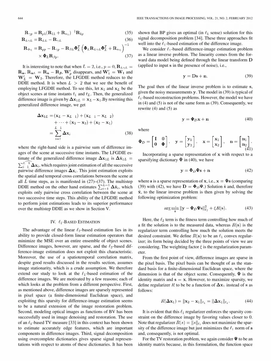
. Therefore, the LFGDIE method reduces to theDDIE method. It is when that we see the benefit ofemploying LFGDIE method. To see this, let and be theobject scenes at time instants and . Then, the generalizeddifference image is given by .By rewriting thisgeneralized difference image, we get

(38)

where the right-hand side is a pairwise sum of difference im-ages of the scene at successive time instants. The LFGDIE es-timate of the generalized difference image is

, which requires joint estimation of all the successivepairwise difference images . This joint estimation exploitsthe spatial and temporal cross correlations between the scene atall time steps, as is manifested in (27)–(37). The multistepDDIE method on the other hand estimates , whichexploits only pairwise cross correlation between the scene attwo successive time steps. This ability of the LFGDIE methodto perform joint estimations leads to its superior performanceover the multistep DDIE as we show in Section V.

IV. -BASED ESTIMATION

The advantage of the linear -based estimation lies in itsability to provide closed-form linear estimation operators thatminimize the MSE over an entire ensemble of object scenes.Difference images, however, are sparse, and the -based dif-ference-image estimation does not exploit this characteristic.Moreover, the use of a spatiotemporal correlation matrix,despite good results discussed in the results section, assumesimage stationarity, which is a crude assumption. We thereforeextend our study to look at the -based estimation of thedifference images. We are motivated by a few reasons; each ofwhich looks at the problem from a different perspective. First,as mentioned above, difference images are sparsely representedin pixel space (a finite-dimensional Euclidean space), andexploiting this sparsity for difference-image estimation seemsto be a natural extension of the image restoration problem.Second, modeling optical images as functions of BV has beensuccessfully used in image denoising and restoration. The useof an -based TV measure [33] in this context has been shownto estimate accurately edge features, which are importantcomponents in difference images. Third, signal decompositionusing overcomplete dictionaries gives sparse signal represen-tations with respect to atoms of these dictionaries. It has been

shown that BP gives an optimal (in sense) solution for thissignal decomposition problem [34]. These three approaches fitwell into the -based estimation of the difference image.

We consider -based difference-image estimation problemas a linear inverse problem. The linearity comes from the for-ward data model being defined through the linear transform(applied to input in the presence of noise), i.e.,

(39)

The goal then of the linear inverse problem is to estimate ,given the noisy measurements . The model in (39) is typical of

-based reconstruction problems. However, the model we havein (4) and (5) is not of the same form as (39). Consequently, werewrite (4) and (5) as

(40)

where

(41)Incorporating a sparse representation of with respect to a

sparsifying dictionary in (40), we have

(42)

where is a sparse representation of , i.e., (comparing(39) with (42), we have .) Solution and, therefore

, to the linear inverse problem is then given by solving thefollowing optimization problem:

(43)

Here, the term is the fitness term controlling how much ofa fit the solution is to the measured data, whereas is theregularizer term controlling how much the solution meets thedesired constraint. We define to be an convex regular-izer; its form being decided by the three points of view we areconsidering. The weighting factor is the regularization param-eter.

From the first point of view, difference images are sparse inthe pixel basis. The pixel basis can be thought of as the stan-dard basis for a finite-dimensional Euclidean space, where thedimension is that of the object scene. Consequently, is theidentity matrix and . However, to maximize sparsity, wedefine regularizer to be be a function of instead of asfollows:

(44)

It is evident that this regularizer enforces the sparsity con-straint on the difference image by favoring values closer to 0.Note that regularizer does not maximize the spar-sity of the difference image but just minimizes the norm ofand, consequently, is not optimal.

For the TV restoration problem, we again consider to be anidentity matrix because, in this formulation, the function space


of BV is defined to be on a discrete finite support. Regularizerfor the TV problem is usually defined to be either

(45)

or

(46)

where and are the isotropic and nonisotropicdiscrete TV regularizers, respectively. The and opera-tors are, respectively, the first-order horizontal and vertical dif-ference operators. Instead of imposing the TV condition on

, however, as in (44), we impose it on the difference image. Now, the regularizer is defined as either

(47)

or

(48)

It is easy to see that a bounded TV assumption for the objectscenes and results in also having BV. Therefore,this modified form does not violate any TV condition.

For the sake of completeness, we also look at the difference-image estimation using an overcomplete sparsifying dictionary

. Specifically, we consider the dictionary to be the symmetricbiorthogonal wavelet transform and the regularizer to be

. This results in the familiar BPDN model, which decom-poses the signal as superposition of the atoms of such thatthe norm of is smallest of all possible decompositions overthe dictionary. However, the set up here is slightly differentfrom traditional BPDN in that we include the sensing matrix

in the model. In traditional BPDN, the sensing matrix isan identity matrix. This modification does not affect the funda-mental problem. The classical BPDN problem can be thoughtof as finding the regularized denoised sparse representation ofthe object scene from the noisy version of the scene. The mod-ified BPDN, on the other hand, finds the regularized denoisedsparse representation of the object scene from measurements ofthe scene using the sensing matrix .

Notice that, by applying (42), we use to estimateand not . Therefore, because of the system con-

straint, there is the additional step of computing from theestimated . Estimating , however, allows us to take advan-tage of the correlation between the object scene at the two timeinstants. By solving (43), with , we compute ajoint estimate of and in the form of . Note that, although

is separable into and , is not. Similarly, in (40), wejointly exploit the scene at the two time instants by consideringregularization terms (44), (47) and (48) that are functions ofthe difference image. Regularizer (44) sparsifies the differenceimage, whereas regularizers (47) and (48) minimize the TV ofthe difference image. In fact, by acting directly on the differenceimage, (40) exploits the correlation between the scene at the twotime instants more strongly than (42).

Extension to estimating sequences of difference images fol-lows directly from the multistep DDIE and, more specifically,(21). We will use the -based techniques in the multistep set-ting. In Section V, we present the performance of these threeapproaches.

A. Learning Sensing and Sparsifying Matrices

Given the above approaches to -based difference-image es-timation, one question that naturally arises is whether we canlearn the optimal and from the available training data. Re-cently, Carvajalino and Sapiro [35] proposed a very interestingscheme to learn simultaneously and using training data.The sparsifying dictionary is assumed to be overcomplete. Thisassumption makes it difficult for us to apply it to our current con-text. Consider the forward model for computing the differenceimage from the object scene at two consecutive time instants.Let the time instants be and . Then, we have

(49)

Here, is a matrix with both and beingvectors. We know that is sparse. Therefore, ideally,

we would like to find such that, when , then .This, however, is not possible using the algorithm proposed byCarvajalino et al. because will be a matrix, which isnot an overcomplete dictionary. Our model has a unique charac-teristic that the forward representation is overcomplete, whereasthe one in the other direction is not. This is unlike most CS signalmodels where overcompleteness of the dictionary in this otherdirection is exploited to achieve sparsity. We can of course com-pute the pseudoinverse of but that is an solution. Wetherefore let be as defined in (41).

V. RESULTS

We now present our results for - and -based difference-image estimation methods. We evaluate the performance usingmeasured video imagery of an urban intersection (i.e., objectscene; see Fig. 1) as the input into a simulation that models com-pressive measurements. We use a Panasonic PV-GS500 videocamcorder to image the object scene. The reason we use conven-tionally imaged data as the truth data and simulate the compres-sive optical imaging system is to achieve flexibility in accuratelyimplementing different sensing matrices . This flexibility isrequired to analyze performance of our proposed sensing ma-trices in estimating sequence of difference images based onand norms. On the other hand, we now have to do computa-tionally what a compressive imaging system will do optically.Consequently, instead of considering the entire 480 720 ob-ject scene, we reduce the problem by looking at the scene in 88, 16 16, and 32 32 blocks. The blocks are stitched togetherto reconstruct the difference image.

To compute the spatial and temporal correlations, we use atraining set comprising 6000 frames of the object scene. Fromeach 480 720 frame, we chose at random 30 blocks of sizes 8

8, 16 16, and 32 32 to give us 180 000 samples to com-pute the spatial autocorrelation matrix. To obtain the spatiotem-poral cross-correlation matrix between object scenes at consec-utive time instants, we select pairs of successive frames and ran-domly select 30 pairs of 8 8, 16 16, and 32 32 blocks


Fig. 4. Eigenspectrum computed from the sample correlation matrix of thedifference images generated from the 6000 training set frames collected usingPanasonic PV-GS500 video camcorder (8 � 8 block size).

from each frame pair, to give us approximately 180 000 samplepairs again. A pair of blocks consists of two blocks each drawnfrom the same region of the two consecutive image frames. Sim-ilarly, we extend the spatiotemporal correlations over longertime lengths for the LFGDIE method where, instead of consid-ering two successive frames, we consider multiple consecutiveframes. Once computed, these correlation matrices are storedfor use in the testing stage.

The use of a spatiotemporal correlation matrix requires theassumption of wide-sense stationarity, which seldom holds inpractice with the possible exception of texture images. Despitethis, there is considerable literature on using second-order sta-tistics to perform various image processing and imaging tasks[36]–[40]. These tasks attempt to reduce the nonstationarityby, e.g., camera tilt compensation or, in the case of eigenfaceanalysis, by face centering and head orientation correction.Other methods have also been suggested for transformingnonstationary images to exhibit stationary characteristics [41],[42]. Such methods are at best approximate and not necessarilysuitable or directly applicable to this paper. Therefore, in thisfirst step toward developing an FSI-based imaging system,we empirically show that our proposed techniques yield goodperformance because of our ability to compress differenceimages by exploiting second-order statistics without artificialattempts at introducing stationarity. To illustrate this compres-sion, we compute the eigenspectrum of the difference imagesgenerated from the 6000 training set frames. Fig. 4 shows thatthis eigenspectrum decays rapidly. This decay is a consequenceof velocities and directions of motion being constrained inmany environments of interest. These constraints can be in theform of roads, sidewalks, trails, corridors, etc. Therefore, if wethink of difference images as a set of translated delta functionsin 2-D, the nonuniqueness of these translations due to the con-strained motion results in the eigenspectrum decay, allowingus to estimate the difference images, with high fidelity, fromcompressive measurements of the scene. The testing data alsocomprise of 6000 frames. These frames are subdivided into100 groups; each comprising the object scene at 60 consecutivetime instants. The testing set includes diverse cases of multipletargets moving at different speeds and directions. All perfor-mance plots (RMSE versus SNR and RMSE versus numberof measurements per block ) in the following analysis havebeen averaged over the 60 time steps and the 100 groups.

Fig. 5. Estimated difference image for SNR � �� dB and� � � using (a)WDPC, (b) Optimal, and (c) truth difference image.

As discussed in Section III, there is no mathematicallytractable optimal sensing matrix. Currently, we con-sider some possible choices for , which were discussed inSection III. To remind the reader, they are PCs, DPCs, WPCs,WDPCs, numerically computed optimal sensing matrix (op-timal) and Gaussian random sensing matrix (GPR). The GPRsensing matrix represents a set of fixed (aymptotically) basisprojections that do not use any a priori information about thescene. The entries of the GPR matrix are Gaussian distributedwith a mean of zero and a variance of one. We also considerthe identity matrix (conventional) to mimic the conventionalimager. We use the conventional imager for baseline perfor-mance comparison. The conventional imager always imagesthe whole scene, i.e., it always makesmeasurements per frame.

A. -Based Difference-Image Estimation

Fig. 5 gives an example of an estimated difference image froma sequence of difference images using the multistep DDIE. Theblock size is 8 8, the SNR value is 10 dB, and the numberof measurements per block is 5. For

-D object scene, translates to 27 000 measure-ments and a compression of measured data by 92.2%. The il-lustrated example has been computed with WDPC and optimalsensing matrices. We see that the performance of the optimalis visually close to that of the truth difference image. More im-portantly, the WDPC also estimates the difference image withgood results. Note that it is much easier and computationallyefficient to compute the WDPC than to numerically find the op-timal sensing matrix. We quantify these results by plotting theroot MSE (RMSE) as a function of SNR. We define RMSE as

RMSE (50)

The normalization is done using the truth difference image.

Fig. 6 plots the multistep DDIE method’s RMSE performanceas a function of SNR for and for the 8 8 blocksize. We see an improvement in quantitative performance with


Fig. 6. RMSE versus SNR plots for the 8� 8 block size. (a)� � �. (b)� �

�.� is the number of measurements per block.

Fig. 7. RMSE versus number of measurements� for SNR � �� dB for the 8� 8 block size.

more measurements, with RMSE significantly decreasing for. Fig. 7, however, shows that this is not true generally

for increasing measurements. With increasing , the perfor-mance first improves and then can degrade. This behavior is adirect result of enforcing the photon count constraint. For small

, any additional measurement adds more information. How-ever, because the total number of photons is fixed, as the numberof measurements increase, additional information per measure-ment goes down. Eventually, the additive noise overwhelms theincremental information, and we see a degradation in perfor-mance for larger . This is true for PC, DPC, and WPC sensingmatrices. However, both WDPC and optimal sensing matricesavoid the degradation in performance with increasing measure-ments because they are optimized for a given SNR. Measure-ments are considered until they improve performance. Once in-formation per measurement begins to be drowned out by noise,the additional measurements are ignored. There seems to be acertain discrepancy between the example estimates in Fig. 5 andthe plots in Fig. 6(b). Although the visually estimated differ-ence image looks good, the plots for have a relativelyhigh RMSE. This discrepancy is because minimization mini-mizes the MSE over an ensemble and does not explicitly enforcesparsity. Consequently, there are small deviations (from the truepixel values) spread out over the whole estimated differenceimage. These small deviations from the truth, when normalizedagainst the sparse truth difference image, bias the RMSE.

In Fig. 6, we can make a few observations about the efficacyof the various sensing matrices. As expected, waterfilling doesimprove performance of both PCs and DPCs by weighting theprojections according to noise statistics. This is more evident

Fig. 8. (a) Performance comparison between single-step and multistep DDIEmethods for � � � and SNR � �� dB using WDPCs. Changing RMSE iscompared over time. (b) Maximum divergence between single-step and multi-step DDIE methods for varying SNR.

in Fig. 6(b), where we take five measurements per block. Nu-merically searching for the optimal sensing matrix further im-proves upon WPCs and WDPCs. The advantage that the latterhave over a numerical search is that they are much simpler tocompute for changing SNR. Therefore, searching for the op-timal solution is reasonable only if improvement in performanceoutweighs the increased computational cost. In Fig. 5, we seethat this not the case. For the sake of completeness, we havealso plotted the RMSE performance of Gaussian random pro-jections (GRPs). We are aware that there is no theoretical frame-work for a nonadaptive GRP to outperform sensing matrices ex-ploiting a priori information. This is experimentally validated inthe plots, which show a GRP to be performing the worst. Lastly,for -based estimation, the conventional imager outperformsall the sensing matrices. This is to be expected as minimizingthe MSE alone does not give an advantage to compressive mea-surements over a conventional imager. We need an additionalconstraint, which, for our case, turns out to be sparsity. We showin the next subsection that we can actually beat the conventionalimager performance when we enforce sparsity via a nonlinearestimation.However, we stress that, as seen in Fig. 5, the qual-itative performance of WDPCs is visually close to that of thetruth difference image. In fact, from a practical perspective, itcan be used to provide a good input to a tracker.

The multistep DDIE, as defined in (21), forms a closed loopbetween the estimate of the scene and the difference image. Asa result, there will be degradation in performance over time. Tograde the performance of the multistep DDIE, we consider aclairvoyant scenario for estimating the sequence of differenceimages. We will refer to this special case as the single-stepDDIE. Assuming we are estimating the difference image of thescene between and , the single-step DDIE always as-sumes perfect knowledge of the scene at as follows:

(51)

Obviously, the single-step DDIE is practically infeasible.However, it does bound the performance of the multistep DDIEand, as such, allows us to evaluate the efficacy of the multistepstrategy. Fig. 8(a) shows the performance comparison betweenthe two for 60 time steps for and SNR dB.Since single-step DDIE assumes perfect knowledge at everystage, its RMSE as a function of time is nearly constant. The


Fig. 9. Eigenspectrum computed from the sample correlation matrix of the dif-ference images generated from the 3500 training set frames from PETS data set(16 � 16 block size).

RMSE for the multistep DDIE is the same as the single-stepDDIE at . With passing time, however, the performanceof multistep DDIE degrades as the RMSE drifts. However,as can be seen, the drift is slow, showing that the multistepDDIE is temporally robust. In Fig. 8(b), we plot the maximumdivergence of the multistep DDIE from the ideal single-stepDDIE for changing the SNR. Maximum divergence is themaximum value by which the multistep method diverges fromthe single-step method over the 60 time steps. The resultingplot is a line with a small slope indicating that the multistepDDIE does not diverge significantly for changing the SNR. Toemphasize further empirically the temporal robustness of themultistep DDIE, we consider a second data set, i.e., the PETS2007 data set. We use two camera views of the same objectscene from this data set, each with 4001 frames. We use 3500frames from the first camera view as the training set. We followthe exact procedure as for the previous data set to compute thespatiotemporal cross-correlation matrix (Fig. 9 illustrates thecompressibility of difference images from this data set in amanner similar to the previous data set). To ensure no overlapbetween the training and the testing sets, the images from theremaining 501 frames in the second camera view are usedfor the testing set. Fig. 10 shows the performance comparisonbetween single-step and multistep DDIE for the PETS data setfor 60 time steps. We see that the RMSE is slightly more thanthat in Fig. 8(a), but the trend is the same. The reason for aslight increase in RMSE is that the training and testing data setare significantly different. In our primary data set, we follow adata collection strategy where the training is done on the sameobject scene that is of interest for target tracking purposes, i.e.,the camera angle is fixed, but the training and testing data setsare defined at different nonoverlapping time intervals. The useof the PETS data set allows us to replicate our results for adifferent scenario where the camera must be trained on onescene and operate on another. Fig. 11 gives an example of anestimated difference image using the PETS testing data set. Thefirst image is the truth difference image at the 50th time step ofan image sequence. The corresponding multistep-DDIE-basedestimated difference image using the optimal sensing matrix isshown in Fig. 11(b) for and SNR dB. The blocksize is 8 8. We see the the visual quality of the estimate is notfar from the truth difference image after 50 time steps.

We now look at the performance of the LFGDIE method forestimating a sequence of difference images. We claimed that the

Fig. 10. PETS data set: Performance comparison between single-step andmulti-step DDIE methods for � � � and SNR � �� dB using WDPC.Changing RMSE is compared over time.

Fig. 11. PETS data set: Multistep-DDIE-based estimated difference image for� � � and SNR � �� dB using the optimal sensing matrix. (a) Truth differ-ence image. (b) Estimated difference image.

LFGDIE will perform better than the multistep DDIE as it isable to exploit temporal correlation between all time instants.Fig. 12 shows that this is indeed the case. RMSE performancehas improved compared with Fig. 6(b). As expected, however,the trends are still the same. The WDPC sensing matrix still out-performs all other candidate sensing matrices with the exceptionof the numerically searched optimal sensing matrix. Until now,we have considered the block size of 8 8. In Fig. 13, we graphthe RMSE performance as a function of SNR for the 16 16block size. We see that, for , there is an improvement inperformance over the 8 8 block size. In fact, the performancewe get for the 16 16 block with is similar to the perfor-mance of the 8 8 block with . Notice that , for16 16 block size, implies 1350 measurements for the wholescene, which translates to less than 0.4% measurements in com-parison with the conventional imager. Thus, we see that, for thelarger block size, we have improved performance with simulta-neously higher compression ratio. Fig. 14, however, shows thatthe amount of improvement in performance we get by goingfrom block size 8 8 to 16 16 is reduced when we go fromblock size 16 16 to 32 32. This happens because any sta-tionarity that holds for the small block sizes of 8 8 beginsto break for larger block sizes. As a result, the spatial structurerepresented by the sample autocorrelation and cross-correlationmatrices obtained from training data does not completely rep-resent the true correlation. The LFGDIE method also has thesame trends as the multistep DDIE. The -based estimation on


Fig. 12. RMSE versus SNR plots for the LFGDIE method. Block size is 8 �8 and� � �.

Fig. 13. RMSE versus SNR performance plots for block size 16� 16, for� �

�.

Fig. 14. Optimal-sensing-matrix based performance comparison between thethree block sizes 8 � 8, 16� 16, and 32� 32 for (a)� � � and (b)� � �.

the other hand does not depend on a stationarity assumption. Itsgoal is to find the best estimate based on the measured data thatenforces the sparsity constraint. In the following subsection, wediscuss the performance of -based estimation methods.

B. -Based Difference-Image Estimation

The advantage of using the norm is that we get preciselinear estimation operators, which allow for quick and easycomputation of the estimate of the difference image. The dis-advantage, however, has to do with the inability to exploit thesparsity of a difference image. Solving the convex optimizationproblem of (43) allows us to overcome this disadvantage.

Here, we consider the PC, DPC, WPC, WDPC, and GRPsensing matrices. All abbreviations are the same as before.Gaussian sensing matrices (i.e., GRP) have been suggested intheory of compressed sensing for measuring data because theyare incoherent with all representation bases. As a result, theyhave become nearly universal in applications of compressedsensing for being able to reconstruct signals of interest without

Fig. 15. Estimated difference image for SNR � �� dB and � � � for(a) sparsity-enforced difference image, (b) TV method, and (c) BPDN method.

Fig. 16. RMSE versus SNR curves for the 8� 8 blocks and for the TV method.(a)� � �. (b)� � �. (c)� � ��. (d)� � ��.

prior knowledge of the signal structure. Fig. 15 shows examplesof the estimated difference image for the 8 8 block size, usingthe three -based methods discussed in Section IV. Visually,all three methods are effective, although TV method performsbetter than the other two. Both isotropic and nonisotropic TVregularizers have similar performance. All the results shownhere are for the nonisotropic TV regularizer. In Fig. 16, we plotthe RMSE performance of the TV method as a function of SNR.The block size is 8 8, and . For ,all sensing matrices have similar performance. In fact, at lowSNR, all sensing matrices perform better than the conventionalimager. Thus, unlike -based estimation, -based methodsare better able to utilize the concentration of energy into afew measurements. This is surprisingly true even for the GRPsensing matrix. At low SNR, there is a higher premium onthe available energy, and as a consequence, a small number ofrandom measurements perform better than the conventional


Fig. 17. WDPC-sensing-matrix RMSE versus SNR curves for the three� -based difference image estimation methods. Block size 8� 8 and � � �.

imager, where the small energy is spread over all themeasurements. For , the curves for different sensingmatrices begin to separate. Yet, the performance of PC andDPC sensing matrices is similar. This is because the -basedestimation does not directly estimate the difference image but,instead, jointly estimates the scene at the two time instants. Asa result, we cannot take advantage of the difference image formthat -based estimation afforded us. We see that waterfillingimproves upon both PC and DPC sensing matrices, but due tothe same reason, the performance of WPC and WDPC sensingmatrices is also similar. The WPC and WDPC sensing matricesgive the best RMSE performance.

In Fig. 17, we compare the performance of the three -basedmethods by looking at the RMSE versus SNR curves for theWDPC sensing matrix. Within the three strategies, we seethat the TV method performs better than the sparsity-enforceddifference-image method and BPDN. However, the improve-ment is small, particularly when compared with the sparsity-en-forced difference-image method. By minimizing the gradient ofthe difference image, the TV method is best able to capture thechanges in intensity across the difference image. On the otherhand, difference images are also sparse; hence, enforcing spar-sity also gives good results. The BPDN method has a higherRMSE compared with the other two strategies. This is to beexpected because, although BPDN also minimizes the normwith respect to a sparsifying basis, it does not directly utilizethe difference image as is done by the regularization term of theother two methods. Instead, the BPDN method computes thejoint sparse representation of the object scene at the two timeinstants. This results in reduced performance. However, as cor-roborated in Fig. 15, the degradation in performance is small.Plotting RMSE as a function of shows us that we are able tobeat the performance of the conventional imager. This is illus-trated in Fig. 18. At low SNR and for smaller measurements, wesee a wide gap in performance between all sensing matrices andthe conventional imager. Note that the conventional imager al-ways makes measurements. As the numberof measurements increase, the performance of all the sensingmatrices begins to degrade. The rate of this degradation is afunction of SNR. It slows down as SNR increases. When theSNR is high, there is no advantage to be obtained from better uti-lizing the energy as there is enough energy for all measurements,and the conventional imager performs the best. Finally, we notethat sensing matrices using a priori information perform better

Fig. 18. RMSE versus number of measurements per block for 8� 8 blocks andfor the TV method. (a) SNR � �� dB. (b) SNR � �� dB. (c) SNR � � dB.(d) SNR � �� dB.

Fig. 19. Performance comparison between the � -based TV method using 8�8 and 32 � 32 blocks. (a) � � �.

than GRP. Looking at the RMSE versus SNR performance ofGRP, we see that it has the most error at all SNRs and for anynumber of measurements. At the same time, RMSE versusplots show that the rate at which the GRP performance degradesis fastest among all sensing matrices. Increasing block size leadsto improved performance for a fewer number of measurementsas a fraction of the total. Unlike the -based method, here, wedo not suffer from the stationarity assumption. In Fig. 19, weplot the performance of the TV method using the WDPC sensingmatrix for 8 8 and 32 32 block sizes. We see that the rateof performance degradation is significantly reduced for the 32

32 block sizes. The improved performance is mainly becausethe sparsity condition holds better for larger block sizes. If theblock size is very small, then even a sparse image might not besparse within that block. However, with increasing block size,we achieve sparsity and, as a result, get better performance.

This trend of improved performance with increasing blocksize augurs well for future practical implementation of our pro-posed strategies. A practical FSI system with the capability tohandle different sensing matrices could optically measure theentire scene at very fast speed. An optical system would not face


the same limitations that we have in terms of simulating mea-surements due to a large scene.

VI. CONCLUSION

In this paper, we have shown - and -based techniques forestimating a sequence of difference images from a sequenceof compressive measurements. We have presented qualitativeand quantitative results to attest that both techniques are ableto estimate successfully the difference images within the FSIparadigm. Each has its advantage. -based techniques giveclosed-form expressions for the linear estimation operators,which are easy to compute. On the other hand, -basedmethods exploit the natural sparsity of the difference image.Within -based techniques, we looked at the multistep DDIEand LFGDIE methods to reconstruct directly the differenceimage from the compressive measurements. For the -basedestimation problem, we looked at three different approachesto the linear inverse problem and compared their performance.We showed that the modified TV method performs the best,although the method that enforced the sparsity conditionperforms only slightly worse. Lastly, we showed that WDPCsensing matrix had the lowest RMSE for both - and -basedmethods, although for the latter WPC did equally well. Theperformance of all sensing matrices that utilized a priori infor-mation was better than the nonadaptive GRP sensing matrix. Infact, from a practical perspective, depending on the SNR andthe number of measurements that can be taken, anyone of themcan be used to provide a decent input to a tracker.

REFERENCES

[1] D. W. Xue and Z. M. Lu, “Difference image watermarking based re-versible image authentication with tampering localization capability,”Int. J. Comput. Sci. Eng. Syst., vol. 2, no. 3, pp. 213–218, 2008.

[2] S. K. Lee, Y. H. Suh, and Y. S. Ho, “Reversible image authenticationbased on watermarking,” in Proc. IEEE Int. Conf. Multimedia Expo.,2006, pp. 1321–1324.

[3] P. B. Heffernan and R. A. Robb, “Difference image reconstruction froma few projections for nondestructive materials inspection,” Appl. Opt.,vol. 24, no. 23, pp. 4105–4110, Dec. 1985.

[4] S. G. Kong, “Classification of interframe difference image blocks forvideo compression,” in Proc. SPIE, 2002, vol. 4668, pp. 29–37.

[5] D. Hahn, V. Daum, J. Hornegger, W. Bautz, and T. Kuwert, “Differ-ence imaging of inter- and intra-ictal spect images for the localizationof seizure onset in epilepsy,” in Proc. IEEE Nucl. Sci. Symp. Conf. Rec.,2007, pp. 4331–4335.

[6] C. Alcock, R. A. Allsman, D. Alves, T. S. Axelrod, A. C. Becker, D.P. Bennett, K. H. Cook, A. J. Drake, K. C. Freeman, K. Griest, M. J.Lehner, S. L. Marshall, D. Minniti, B. A. Peterson, M. R. Pratt, P. J.Quinn, C. W. Stubbs, W. Sutherland, A. Tomaney, T. Vandehei, and D.L. Welch, “Difference image analysis of galactic microlensing. I. dataanalysis,” Astrophys. J., vol. 521, no. 2, pp. 602–612, Aug. 1999.

[7] L. Bruzzone and D. F. Prieto, “Automatic analysis of the differenceimage for unsupervised change detection,” IEEE Trans. Geosci. Re-mote Sens., vol. 38, no. 3, pp. 1171–1182, May 2000.

[8] M. A. Neifeld and P. Shankar, “Feature-specific imaging,” Appl. Opt.,vol. 42, no. 17, pp. 3379–3389, Jun. 2003.

[9] S. Tucker, W. T. Cathey, and J. Edward Dowski, “Extended depth offield and aberration control for inexpensive digital microscope sys-tems,” Opt. Exp., vol. 4, no. 11, pp. 467–474, May 1999.

[10] S. Prasad, “Information capacity of a seeing-limited imaging system,”Opt. Commun., vol. 177, no. 1–6, pp. 119–134, Apr. 2000.

[11] E. Clarkson and H. H. Barrett, “Approximations to ideal-observer per-formance on signal-detection tasks,” Appl. Opt., vol. 39, no. 11, pp.1783–1793, Apr. 2000.

[12] W.-C. Chou, M. A. Neifeld, and R. Xuan, “Information-based opticaldesign for binary-valued imagery,” Appl. Opt., vol. 39, no. 11, pp.1731–1742, Apr. 2000.

[13] A. Ashok and M. Neifeld, “Information-based analysis of simple in-coherent imaging systems,” Opt. Exp., vol. 11, no. 18, pp. 2153–2162,Sep. 2003.

[14] M. P. Christensen, G. W. Euliss, M. J. McFadden, K. M. Coyle,P. Milojkovic, M. W. Haney, J. van der Gracht, and R. A. Athale,“ACTIVE-EYES: An adaptive pixel-by-pixel image-segmentationsensor architecture for high-dynamic-range hyperspectral imaging,”Appl. Opt., vol. 41, no. 29, pp. 6093–6103, Oct. 2002.

[15] D. L. Marks, R. Stack, A. J. Johnson, D. J. Brady, and D. C. Munson,“Cone-beam tomography with a digital camera,” Appl. Opt., vol. 40,no. 11, pp. 1795–1805, Apr. 2001.

[16] Z. Liu, M. Centurion, G. Panotopoulos, J. Hong, and D. Psaltis, “Holo-graphic recording of fast events on a CCD camera,” Opt. Lett., vol. 27,no. 1, pp. 22–24, Jan. 2002.

[17] P. Potuluri, M. Fetterman, and D. Brady, “High depth of field micro-scopic imaging using an interferometric camera,” Opt. Exp., vol. 8, no.11, pp. 624–630, May 2001.

[18] S. M. Kay, Fundamentals of Statistical Processing. EnglewoodCliffs, NJ: Prentice-Hall, 1993.

[19] E. J. Candès, J. K. Romberg, and T. Tao, “Robust uncertainty prin-ciples: Exact signal reconstruction from highly incomplete frequencyinformation,” IEEE Trans. Inf. Theory vol. 52, no. 2, pp. 489–509, Feb.2006 [Online]. Available: http://doi.ieeecomputersociety.org/10.1109/TIT.2005.862083

[20] E. J. Candès and T. Tao, “Near-optimal signal recovery from randomprojections: Universal encoding 2strategies?,” IEEE Trans. Inf. Theoryvol. 52, no. 12, pp. 5406–5425, Dec. 2006 [Online]. Available: http://doi.ieeecomputersociety.org/10.1109/TIT.2006.885507

[21] E. J. Candès and T. Tao, “Decoding by linear programming,” IEEETrans. Inf. Theory vol. 51, no. 12, pp. 4203–4215, Dec. 2005 [Online].Available: http://doi.ieeecomputersociety.org/10.1109/TIT.2005.858979

[22] E. J. Candès, J. K. Romberg, and T. Tao, “Signal recovery from incom-plete and inaccurate measurements,” Commun. Pure Appl. Math., vol.59, no. 8, pp. 1207–1223, 2005.

[23] E. J. Candès and J. K. Romberg, “Quantitative robust uncertainty prin-ciples and optimally sparse decompositions,” Found. Comput. Math.vol. 6, no. 2, pp. 227–254, Apr. 2006 [Online]. Available: http://dx.doi.org/10.1007/s10208-004-0162-x

[24] D. L. Donoho, “Compressed sensing,” IEEE Trans. Inf. Theory, vol.52, no. 4, pp. 1289–1306, Apr. 2006.

[25] S. Uttam, N. A. Goodman, and M. A. Neifeld, “Direct reconstructionof difference images from optimal spatial-domain projections,” in Proc.SPIE, 2008, vol. 7096, pp. 709 608-1–709 608-6.

[26] M. B. Wakin, J. N. Laska, M. F. Duarte, D. Baron, S. Sarvotham, D.Takhar, K. F. Kelly, and R. G. Baraniuk, “An architecture for com-pressive imaging,” in Proc. IEEE Int. Conf. Image Process., 2006, pp.1273–1276.

[27] V. Cehver, A. Sankaranarayanan, M. F. Duarte, D. Reddy, R. G. Bara-niuk, and R. Chellappa, “Compressive sensing for background subtrac-tion,” in Proc. 10th Eur. Conf. Comput. Vis., 2008, pp. 155–168.

[28] V. Cevher, M. F. Duarte, C. Hedge, and R. Baraniuk, “Sparse signalrecovery using Markov random fields,” presented at the Neural In-formation Processing Systems (NIPS), Vancouver, BC, Canada, 2008,EPFL-CONF-151 469, unpublished.

[29] M. Piccardi, “Background subtraction techniques: A review,” in Proc.IEEE Syst., Man Cybern., 2004, vol. 4, pp. 3099–3104.

[30] M. A. Neifeld and J. Ke, “Optical architectures for compressiveimaging,” Appl. Opt., vol. 46, no. 22, pp. 5293–5303, Aug. 2007.

[31] T. M. Cover and J. A. Thomas, Elements of Information Theory.Hoboken, NJ: Wiley, 2006.

[32] W. Wenzel and K. Hamacher, “A stochastic tunneling approach forglobal minimization,” Phys. Rev. Lett., vol. 82, no. 15, pp. 3003–3007,1999.

[33] S. Osher, L. Rudin, and E. Fatemi, “Nonlinear total variation basednoise removal algorithms,” Phys. D., vol. 60, no. 1–4, pp. 259–268,Nov. 1992.

[34] S. S. Chen, D. L. Donoho, and M. A. Saunders, “Atomic decompositionby basis pursuit,” SIAM Rev., vol. 43, no. 1, pp. 129–159, 2001.

[35] J. M. D. Carvajalino and G. Sapiro, “Learning to sense sparse signals:Simultaneous sensing matrix and sparsifying dictionary optimization,”IEEE Trans. Image Process., vol. 18, no. 7, pp. 1395–1408, Jul. 2009.


[36] L. Malagón-Borja and O. Fuentes, “An object detection system usingimage reconstruction with pca,” in Proc. Comput. Robot Vis., Can.Conf., 2005, pp. 2–8.

[37] M. Turk and A. Pentland, “Face recognition using Eigenfaces,” in Proc.IEEE Conf. Comput. Vis. Pattern Recognit., 1991, pp. 586–591.

[38] A. Pentland, B. Moghaddam, and T. Starner, View-based and modulareigenspaces for face recognition MIT, Cambridge, MA, Tech. Rep.,1994.

[39] H. Moon and P. Phillips, “Computational and performance aspects ofPCA-based face recognition algorithms,” Perception, vol. 30, no. 3, pp.303–321, Jan. 2001.

[40] H. S. Pal, D. Ganotra, and M. A. Neifeld, “Face recognition by usingfeature-specific imaging,” Appl. Opt., vol. 44, no. 18, pp. 3784–3794,Jun. 2005.

[41] R. Chin, “Restoration of images with nonstationary mean and autocor-relation,” in Proc. ICASSP, Apr. 1988, vol. 2, pp. 1008–1011.

[42] R. N. Strickland, “Transforming images into block stationary be-havior,” Appl. Opt., vol. 22, no. 10, pp. 1462–1473, May 1983.

Shikhar Uttam (S’00–M’10) received the B.Tech.degree from Jamia Millia Islamia, New Delhi, India,in 2002, and the M.S. and Ph.D. degrees from theUniversity of Arizona, Tucson, in 2006 and 2010, re-spectively, all in electrical engineering.

From 2005 to 2010, he was a member with theLaboratory for Sensor and Array Processing, De-partment of Electrical and Computer Engineering,University of Arizona. He is currently a PostdoctoralResearch Associate with the Biomedical Optical andImaging Laboratory, Department of Medicine and

with the Department of Bioengineering, University of Pittsburgh, Pittsburgh,PA. His current research interests include computational imaging, quantitativephase microscopy, spectral imaging, diffraction tomography, color-based imageprocessing, and machine learning.

Dr. Uttam is a member of SPIE and SIAM.

Nathan A. Goodman (S’98–M’02–SM’07) receivedthe B.S., M.S., and Ph.D. degrees from the Univer-sity of Kansas, Lawrence, in 1995, 1997, and 2002,respectively, all in electrical engineering.

From 1996 to 1998, he was a Radio-FrequencySystems Engineer with Texas Instruments, Dallas.From 1998 to 2002, he was a Graduate Research As-sistant with the Radar Systems and Remote SensingLaboratory, University of Kansas. In 2009–2010,he was a Visiting Senior Research Engineer withthe Georgia Tech Research Institute, Smyrna, GA.

He is currently an Associate Professor with the Department of Electrical andComputer Engineering, University of Arizona, Tucson. Within the department,he directs the Laboratory for Sensor and Array Processing. His researchinterests include novel system and processing concepts for radar, includingsparse-array and multistatic radar systems, adaptive waveform transmission fortarget recognition and air-to-ground surveillance, and compressed sensing forradar.

Dr. Goodman was a Technical Co-chair for the 2011 IEEE Radar Conferenceand will be the Finance Chair for the 2012 IEEE Sensor Array and MultichannelSignal Processing Workshop. He has served as a Reviewer for numerous jour-nals and conferences and currently serves as a Deputy Editor-in-Chief for Else-vier Digital Signal Processing. He was a recipient of the Madison A. and LilaSelf Graduate Fellowship upon returning to the University of Kansas for Ph.D.studies in 1998, the IEEE 2001 International Geoscience and Remote SensingSymposium Interactive Session Prize Paper Award, and a Best Paper Award atthe 2008 Army Science Conference.

Mark A. Neifeld (S’84–M’91) received the B.S.E.E.degree from the Georgia Institute of Technology, At-lanta, in 1985 and the M.S. and Ph.D. degrees fromthe California Institute of Technology, Pasadena, in1987 and 1991, respectively.

In 1991, he joined the Faculty of the Departmentof Electrical and Computer Engineering and the Op-tical Sciences Center, University of Arizona, Tucson.He is the author or coauthor of more than 100 journalarticles and more than 250 conference papers in theareas of optical communications and storage, coding

and signal processing, and optical imaging and processing systems. His currentresearch interests include information- and communication-theoretic methods inimage processing, nontraditional imaging techniques that exploit the joint opti-mization of optical and postprocessing degrees of freedom, coding and modu-lation for fiber and free-space optical communications, and applications of slowand fast light.

Dr. Neifeld is a Fellow of the Optical Society of America and a member ofSPIE and APS. He has served on the organizing committees of numerous con-ferences and symposia. He has also been a two-term Topical Editor for AppliedOptics and a three-time Guest Editor of special issues of Applied Optics.

Documents

Feature-Specific Difference Imaging