arX

iv:1

311.

5623

v2 [

astr

o-ph

.HE

] 9

Dec

201

3

Fermi-LAT Observations of the Gamma-ray Burst

GRB 130427A

1

M. Ackermann1, M. Ajello2, K. Asano3, W. B. Atwood4,M. Axelsson5,6,7, L. Baldini8, J. Ballet9, G. Barbiellini10,11,

M. G. Baring12, D. Bastieri13,14, K. Bechtol15, R. Bellazzini16,E. Bissaldi17, E. Bonamente18,19, J. Bregeon16, M. Brigida20,21,

P. Bruel22, R. Buehler1, J. Michael Burgess23, S. Buson13,14,G. A. Caliandro24, R. A. Cameron15, P. A. Caraveo25, C. Cecchi18,19,

V. Chaplin23, E. Charles15, A. Chekhtman26, C. C. Cheung27,

J. Chiang15,∗, G. Chiaro14, S. Ciprini28,29, R. Claus15,W. Cleveland30, J. Cohen-Tanugi31, A. Collazzi32, L. R. Cominsky33,

V. Connaughton23, J. Conrad34,6,35,36, S. Cutini28,29, F. D’Ammando37,A. de Angelis38, M. DeKlotz39, F. de Palma20,21, C. D. Dermer27,∗,

R. Desiante10, A. Diekmann40, L. Di Venere15, P. S. Drell15,A. Drlica-Wagner15, C. Favuzzi20,21, S. J. Fegan22, E. C. Ferrara41,

J. Finke27, G. Fitzpatrick42, W. B. Focke15, A. Franckowiak15,Y. Fukazawa43, S. Funk15, P. Fusco20,21, F. Gargano21,

N. Gehrels41, S. Germani18,19, M. Gibby40, N. Giglietto20,21,

M. Giles40, F. Giordano20,21, M. Giroletti37, G. Godfrey15,J. Granot44, I. A. Grenier9, J. E. Grove27, D. Gruber45,

S. Guiriec41,32, D. Hadasch24, Y. Hanabata43, A. K. Harding41,M. Hayashida15,46, E. Hays41, D. Horan22, R. E. Hughes47,

Y. Inoue15, T. Jogler15, G. Johannesson48, W. N. Johnson27,T. Kawano43, J. Knodlseder49,50, D. Kocevski15, M. Kuss16,J. Lande15, S. Larsson34,6,5, L. Latronico51, F. Longo10,11,

F. Loparco20,21, M. N. Lovellette27, P. Lubrano18,19, M. Mayer1,M. N. Mazziotta21, J. E. McEnery41,52, P. F. Michelson15, T. Mizuno53,

A. A. Moiseev54,52, M. E. Monzani15, E. Moretti7,6, A. Morselli55,I. V. Moskalenko15, S. Murgia15, R. Nemmen41, E. Nuss31,

M. Ohno43, T. Ohsugi53, A. Okumura15,56, N. Omodei15,∗,M. Orienti37, D. Paneque57,15, V. Pelassa23, J. S. Perkins41,58,54,

M. Pesce-Rollins16, V. Petrosian15, F. Piron31, G. Pivato14,T. A. Porter15,15, J. L. Racusin41, S. Raino20,21, R. Rando13,14,M. Razzano16,4, S. Razzaque59, A. Reimer60,15, O. Reimer60,15,

S. Ritz4, M. Roth61, F. Ryde7,6, A. Sartori25,

2

P. M. Saz Parkinson4, J. D. Scargle62, A. Schulz1, C. Sgro16,E. J. Siskind63, E. Sonbas41,64,30, G. Spandre16, P. Spinelli20,21,

H. Tajima15,56, H. Takahashi43, J. G. Thayer15, J. B. Thayer15,D. J. Thompson41, L. Tibaldo15, M. Tinivella16, D. F. Torres24,65,

G. Tosti18,19, E. Troja41,52, T. L. Usher15, J. Vandenbroucke15,V. Vasileiou31, G. Vianello15,66,∗, V. Vitale55,67, B. L. Winer47,K. S. Wood27, R. Yamazaki68, G. Younes30,69, H.-F. Yu45,

S. Zhu52,∗, P. N. Bhat23, M. S. Briggs23, D. Byrne42,S. Foley42,45, A. Goldstein23, P. Jenke23, R. M. Kippen70,

C. Kouveliotou69, S. McBreen42,45, C. Meegan23, W. S. Paciesas30,R. Preece23, A. Rau45, D. Tierney42, A. J. van der Horst71,

A. von Kienlin45, C. Wilson-Hodge69, S. Xiong23,∗, G. Cusumano72,V. La Parola72, J. R. Cummings41,73

3

1. Deutsches Elektronen Synchrotron DESY, D-15738 Zeuthen, Germany

2. Space Sciences Laboratory, 7 Gauss Way, University of California,

Berkeley, CA 94720-7450, USA

3. ICRR

4. Santa Cruz Institute for Particle Physics, Department of Physics

and Department of Astronomy and Astrophysics, University of California

at Santa Cruz, Santa Cruz, CA 95064, USA

5. Department of Astronomy, Stockholm University, SE-106 91 Stockholm,

Sweden

6. The Oskar Klein Centre for Cosmoparticle Physics, AlbaNova, SE-106

91 Stockholm, Sweden

7. Department of Physics, Royal Institute of Technology (KTH), AlbaNova,

SE-106 91 Stockholm, Sweden

8. Universita di Pisa and Istituto Nazionale di Fisica Nucleare,

Sezione di Pisa I-56127 Pisa, Italy

9. Laboratoire AIM, CEA-IRFU/CNRS/Universite Paris Diderot, Service

d’Astrophysique, CEA Saclay, 91191 Gif sur Yvette, France

10. Istituto Nazionale di Fisica Nucleare, Sezione di Trieste, I-34127

Trieste, Italy

11. Dipartimento di Fisica, Universita di Trieste, I-34127 Trieste,

Italy

12. Rice University, Department of Physics and Astronomy, MS-108,

P. O. Box 1892, Houston, TX 77251, USA

13. Istituto Nazionale di Fisica Nucleare, Sezione di Padova, I-35131

Padova, Italy

14. Dipartimento di Fisica e Astronomia “G. Galilei”, Universita

di Padova, I-35131 Padova, Italy

15. W. W. Hansen Experimental Physics Laboratory, Kavli Institute for

Particle Astrophysics and Cosmology, Department of Physics and SLAC

National Accelerator Laboratory, Stanford University, Stanford, CA

94305, USA

16. Istituto Nazionale di Fisica Nucleare, Sezione di Pisa, I-56127

Pisa, Italy

4

17. Istituto Nazionale di Fisica Nucleare, Sezione di Trieste, and

Universita di Trieste, I-34127 Trieste, Italy

18. Istituto Nazionale di Fisica Nucleare, Sezione di Perugia,

I-06123 Perugia, Italy

19. Dipartimento di Fisica, Universita degli Studi di Perugia,

I-06123 Perugia, Italy

20. Dipartimento di Fisica “M. Merlin” dell’Universita e del

Politecnico di Bari, I-70126 Bari, Italy

21. Istituto Nazionale di Fisica Nucleare, Sezione di Bari, 70126 Bari,

Italy

22. Laboratoire Leprince-Ringuet, Ecole polytechnique, CNRS/IN2P3,

Palaiseau, France

23. Center for Space Plasma and Aeronomic Research (CSPAR), University

of Alabama in Huntsville, Huntsville, AL 35899, USA

24. Institut de Ciencies de l’Espai (IEEE-CSIC), Campus UAB, 08193

Barcelona, Spain

25. INAF-Istituto di Astrofisica Spaziale e Fisica Cosmica, I-20133

Milano, Italy

26. Center for Earth Observing and Space Research, College of Science,

George Mason University, Fairfax, VA 22030, resident at Naval Research

Laboratory, Washington, DC 20375, USA

27. Space Science Division, Naval Research Laboratory, Washington,

DC 20375-5352, USA

28. Agenzia Spaziale Italiana (ASI) Science Data Center, I-00044

Frascati (Roma), Italy

29. Istituto Nazionale di Astrofisica - Osservatorio Astronomico

di Roma, I-00040 Monte Porzio Catone (Roma), Italy

30. Universities Space Research Association (USRA), Columbia,

MD 21044, USA

31. Laboratoire Univers et Particules de Montpellier, Universite

Montpellier 2, CNRS/IN2P3, Montpellier, France

32. NASA Postdoctoral Program Fellow, USA

33. Department of Physics and Astronomy, Sonoma State University,

Rohnert Park, CA 94928-3609, USA

5

34. Department of Physics, Stockholm University, AlbaNova, SE-106 91

Stockholm, Sweden

35. Royal Swedish Academy of Sciences Research Fellow, funded by a grant

from the K. A. Wallenberg Foundation

36. The Royal Swedish Academy of Sciences, Box 50005, SE-104 05

Stockholm, Sweden

37. INAF Istituto di Radioastronomia, 40129 Bologna, Italy

38. Dipartimento di Fisica, Universita di Udine and Istituto Nazionale

di Fisica Nucleare, Sezione di Trieste, Gruppo Collegato di Udine,

I-33100 Udine, Italy

39. Stellar Solutions Inc., 250 Cambridge Avenue, Suite 204, Palo Alto,

CA 94306, USA

40. Jacobs Technology, Huntsville, AL 35806, USA

41. NASA Goddard Space Flight Center, Greenbelt, MD 20771, USA

42. University College Dublin, Belfield, Dublin 4, Ireland

43. Department of Physical Sciences, Hiroshima University,

Higashi-Hiroshima, Hiroshima 739-8526, Japan

44. Department of Natural Sciences, The Open University of Israel,

1 University Road, POB 808, Ra’anana 43537, Israel

45. Max-Planck Institut fur extraterrestrische Physik, 85748 Garching,

Germany

46. Department of Astronomy, Graduate School of Science, Kyoto University,

Sakyo-ku, Kyoto 606-8502, Japan

47. Department of Physics, Center for Cosmology and Astro-Particle Physics,

The Ohio State University, Columbus, OH 43210, USA

48. Science Institute, University of Iceland, IS-107 Reykjavik, Iceland

49. CNRS, IRAP, F-31028 Toulouse cedex 4, France

50. GAHEC, Universite de Toulouse, UPS-OMP, IRAP, Toulouse, France

51. Istituto Nazionale di Fisica Nucleare, Sezione di Torino, I-10125

Torino, Italy

52. Department of Physics and Department of Astronomy, University of

Maryland, College Park, MD 20742, USA

6

53. Hiroshima Astrophysical Science Center, Hiroshima University,

Higashi-Hiroshima, Hiroshima 739-8526, Japan

54. Center for Research and Exploration in Space Science and Technology

(CRESST) and NASA Goddard Space Flight Center, Greenbelt, MD 20771, USA

55. Istituto Nazionale di Fisica Nucleare, Sezione di Roma “Tor Vergata”,

I-00133 Roma, Italy

56. Solar-Terrestrial Environment Laboratory, Nagoya University,

Nagoya 464-8601, Japan

57. Max-Planck-Institut fur Physik, D-80805 Munchen, Germany

58. Department of Physics and Center for Space Sciences and Technology,

University of Maryland Baltimore County, Baltimore, MD 21250, USA

59. University of Johannesburg, Department of Physics, University of

Johannesburg, Auckland Park 2006, South Africa,

60. Institut fur Astro- und Teilchenphysik and Institut fur

Theoretische Physik, Leopold-Franzens-Universitat Innsbruck, A-6020

Innsbruck, Austria

61. Department of Physics, University of Washington, Seattle, WA 98195-1560,

USA

62. Space Sciences Division, NASA Ames Research Center, Moffett Field,

CA 94035-1000, USA

63. NYCB Real-Time Computing Inc., Lattingtown, NY 11560-1025, USA

64. Adıyaman University, 02040 Adıyaman, Turkey

65. Institucio Catalana de Recerca i Estudis Avancats (ICREA),

Barcelona, Spain

66. Consorzio Interuniversitario per la Fisica Spaziale (CIFS),

I-10133 Torino, Italy

67. Dipartimento di Fisica, Universita di Roma “Tor Vergata”,

I-00133 Roma, Italy

68. Department of Physics and Mathematics, Aoyama Gakuin University,

Sagamihara, Kanagawa, 252-5258, Japan

69. NASA Marshall Space Flight Center, Huntsville, AL 35812, USA

70. Los Alamos National Laboratory, Los Alamos, NM 87545, USA

71. Astronomical Institute ”Anton Pannekoek” University of Amsterdam,

Postbus 94249 1090 GE Amsterdam, Netherlands

7

72. INAF - Istituto di Astrofisica Spaziale e Fisica Cosmica,

Via U. La Malfa 153, I-90146 Palermo, Italy

73. University of Maryland, Baltimore County / Center for Research and

Exploration in Space Science and Technology

∗To whom correspondence should be addressed. Email:

sjzhu@umd.du (S.J.Z.); jchiang@slac.stanford.edu (J.C.);

charles.dermer@nrl.navy.mil (C.D.D.); nicola.omodei@stanford.edu (N.O.);

giacomov@slac.stanford.edu (G.V.); Shaolin.Xiong@uah.edu (S.X.).

The observations of the exceptionally bright gamma-ray burst (GRB)130427A by the Large Area Telescope aboard the Fermi Gamma-raySpace Telescope provide constraints on the nature of such unique as-trophysical sources. GRB 130427A had the largest fluence, highest-energy photon (95 GeV), longest γ-ray duration (20 hours), andone of the largest isotropic energy releases ever observed from aGRB. Temporal and spectral analyses of GRB 130427A challengethe widely accepted model that the non-thermal high-energy emis-sion in the afterglow phase of GRBs is synchrotron emission radiatedby electrons accelerated at an external shock.

Introduction

Gamma-ray bursts (GRBs) are thought to originate from collapsing massive stars ormerging compact objects (such as neutron stars or black holes), and are associated withthe formation of black holes in distant galaxies.

GRB 130427A was detected by both the Large Area Telescope (LAT) and the Gamma-ray Burst Monitor (GBM) aboard the Fermi Gamma-ray Space Telescope. The LAT isa pair-conversion telescope that observes photons from 20 MeV to >300 GeV with a2.4 steradian field of view (1). The GBM consists of 12 sodium iodide (NaI, 8 keV– 1 MeV) and 2 bismuth germanate (BGO, 200 keV – 40 MeV) detectors, positionedaround the spacecraft to view the entire unocculted sky (2).

In the standard model of GRBs, the blast wave that produces the initial, bright promptemission later collides with the external material surrounding the GRB (the circumburstmedium) and creates shocks (see, e.g., (3)). These external shocks accelerate chargedparticles, which produce photons through synchrotron radiation. Until this burst, thehigh-energy emission from LAT-detected GRBs had been well described by this model,

8

but GRB 130427A challenges this widely accepted model. In particular, the maximumpossible photon energy prescribed by this model is surpassed by the the late-time high-energy photons detected by the LAT. The LAT detected high-energy γ-ray emission fromthis burst for almost a day, including a 95 GeV photon (which was emitted at 128 GeVin the rest frame at redshift z = 0.34 (4)) a few minutes after the burst began and a32 GeV photon (43 GeV in the rest frame) after more than 9 hours. These are moreenergetic and detected at considerably later times than the previous record holder, an18 GeV photon detected by the Energetic Gamma Ray Experiment Telescope (EGRET)aboard the Compton Gamma Ray Observatory more than 90 minutes after GRB 940217began (5).

Observations

At 07:47:06.42 UTC on 27 April 2013 (T0), while Fermi was in the regular survey mode,the GBM triggered on GRB 130427A. The burst was sufficiently hard and intense toinitiate an Autonomous Repoint Request (6), a spacecraft slewing maneuver that keepsthe burst within the LAT field of view for 2.5 hours, barring Earth occultation. At thetime of the GBM trigger, the Swift Burst Alert Telescope (BAT) was slewing between twopre-planned targets, and triggered on the ongoing burst at 07:47:57.51 UTC immediatelyafter the slew completed (7), 51.1 s after the GBM trigger. The CARMA millimeter-waveobservatory localized this burst to (R.A., Dec.) = (173.1367, 27.6989) (J2000) with a0.4′′ uncertainty (8). The Rapid Telescopes for Optical Response (RAPTOR) detectedbright optical emission from the GRB, peaking at a red-band magnitude of R = 7.03 ±0.03 around the GBM trigger time before fading to R∼10 about 80 seconds later (9).The Gemini-North observatory reported a redshift of z = 0.34 (4), and an underlyingsupernova has been detected (10). A total of 58 observatories have reported observationsof this burst as of September 2013.

At the time of the GBM trigger, the GRB was 47.3 from the LAT boresight, wellwithin the LAT field of view. The Autonomous Repoint Request brought the burstto 20.1 from the LAT boresight based on the position calculated by the GBM flightsoftware. It remained in the LAT field of view for 715 s until it became occulted by theEarth, re-emerging from Earth occultation at T0 + 3135 s. Within the first ∼80 ks afterthe trigger, the LAT detected more than 500 photons with energies >100 MeV associatedwith the GRB; the previous record holder was GRB 090902B, with ∼200 photons (11).In addition, the LAT detected 15 photons with energies >10 GeV (compared to only 3photons for GRB 090902B). Using the LAT Low Energy (LLE) event selection (12), whichconsiderably increases the LAT effective collecting area to lower-energy γ-rays down to10 MeV (with adequate energy reconstruction down to 30 MeV) (13, 14), thousands ofcounts above background were detected between T0 and T0 + 100 s.

9

Temporal characteristics

The temporal profile of the emission from GRB 130427A varies strongly with energy from10 keV to ∼100 GeV (Fig. 1 and Fig. 2). The GBM light curves consist of an initial peakwith a few-second duration, a much brighter multipeaked emission episode lasting ∼10 s,and a dim, broad peak at T0 + 120 s, which fades to an undetectable level after ∼300 s(also seen in the Swift light curve (7)).

The triggering pulse observed in the LLE (>10 MeV) light curve is more sharplypeaked than the NaI- and BGO-detected emission at T0. The LLE light curve betweenT0 + 4 s and T0 + 12 s exhibits a multipeaked structure. Some of these peaks havecounterparts in the GBM energy range, although the emission episodes are not perfectlycorrelated (e.g., the sharp spike in the LLE light curve at T0+9.5 s is not relatively brightin the GBM light curves) because of the spectral evolution with energy.

The LAT-detected emission, however, does not appear to be temporally correlatedwith either the LLE or GBM emission beyond the initial spike at T0. Photons withenergies >1 GeV are first observed ∼10 s after T0, after the brightest GBM emission hasended, consistent with a delayed onset of the high-energy emission (13). The delayedonset is not caused by a progressively increasing LAT acceptance due to slewing, becausethe slew started at T0 + 33 s. Instead, it reflects the true evolution of the GRB emission.

GRB spectra are generally well described by phenomenological models such as theBand function (15) or the smoothly broken power law (SBPL (16)). For the brightestLAT bursts, the onset of the GeV emission is delayed with respect to the keV-MeVemission and can be fit by an additional power-law component (13). This additionalcomponent usually becomes significant while the keV-MeV emission is still bright.

For GRB 130427A, however, the extra power-law component becomes significant onlyafter the GBM-detected emission has faded (Fig. 3). During the initial peak (T0 − 0.1 sto T0 + 4.5 s), there are only a few LAT-detected photons, and the emission is well-fit byan SBPL. For the brightest part of the burst (T0+4.5 s to T0+11.5 s), we did not use theGBM-detected emission because of the substantial systematic effects caused by extremelyhigh flux (SOM); however, there are no photons with energies greater than 1 GeV in thistime interval, and the energy spectrum >30 MeV is well described by a single powerlaw without a break (Fig. 3) (note that the LAT did not suffer from any pile up issues).Photons with energies greater than 1 GeV are detected in the last time interval (T0+11.5 sto T0 + 33.0 s), including a 73 GeV photon at T0 + 19 s. Unlike other bright LAT bursts,the LAT-detected emission from GRB 130427A appears to be temporally distinct fromthe GBM-detected emission, suggesting that the GeV and keV-MeV photons arise fromdifferent emission regions or mechanisms.

10

Temporally extended high-energy emission

To characterize the temporally extended high-energy emission, we performed an unbinnedmaximum likelihood analysis of the LAT >100 MeV data. We modeled the LAT photonspectrum as a power law with a spectral index α (i.e., the spectrum N(E) ∝ Eα). Wefound evidence of spectral evolution during the high-energy emission. In contrast toanother study (17), that used longer time intervals in the spectral fits, we found that theLAT >100 MeV spectrum of the GRB is well described by a power law at all times, butwith a varying spectral index (SOM).

Fig. 2 shows the behavior of the temporally extended LAT emission. During the firstpulse around T0, the >100 MeV emission is faint and soft; the pulse contains only a fewphotons, and their energies are all <1 GeV. This is followed by a period during whichthere is no significant >100 MeV emission, while the GBM emission is at its brightest.Starting at ∼T0 +5 s, the >100 MeV emission is detectable again, but remains dim until∼T0 + 12 s. The spectral index fluctuates between α ∼ −2.5 and α ∼ −1.7. At latetimes (>T0 +300 s), we measured typical spectral indices of α ∼ −2, consistent with theindices of other LAT bursts (13). During the time intervals with the hardest spectra, theLAT observed the highest energy photons — such as the 73 GeV photon at T0+19 s andthe record breaking 95 GeV photon at T0 + 244 s — which severely restrict the possiblemechanisms that could generate the high-energy afterglow emission (Table S2).

The temporally extended photon flux light curve is better fit by a broken power lawthan a power law. We found a break after a few hundred seconds, with the temporal indexsteepening from −0.85 ± 0.08 to −1.35 ± 0.08 (χ2/dof = 36/19 for a single power law,16/17 for a broken power law). In contrast, a break is not statistically preferred in theenergy flux light curve (χ2/dof = 14/18 for a single power law, 13/17 for a broken powerlaw), probably because of the larger statistical uncertainties. For a single power-law fitto the energy flux light curve, we found a temporal index of −1.17±0.06, consistent withother LAT bursts (13).

The GBM and Swift energy flux light curves are also shown in Fig. 2. The Swift X-RayTelescope (XRT) began observing the burst at T0+190 s; the reported XRT+BAT (0.3 –10 keV) light curve is a combination of XRT data and BAT-detected emission (15 – 150keV) extrapolated down into the energy range of the XRT. The XRT+BAT light curveshows the unabsorbed flux in the 0.3 – 10 keV range (7). During the initial part of theburst, the GBM (10 keV – 10 MeV) light curve peaks earlier than both the XRT+BAT(0.3 – 10 keV) and LAT (>100 MeV) light curves. The GBM light curve peaks again at∼ T0 + 120 s (see also (7)), while the LAT light curve shows a sharp and hard peak atT0 + 200 s. The BAT+XRT light curve peaks again as well at the same time as the LATlight curve, but the peak is much broader.

11

Interpretation

The energetics of GRB 130427A place it among the brightest LAT bursts. For GRB130427A, the 10 keV – 20 MeV fluence measured with the GBM in the 400 s followingT0 is ∼ 4.2 × 10−3 erg cm−2. The issue with pulse pileup and the uncertainties in thecalibration of the GBM detectors contribute to a systematic error which we estimate tobe less than 20%; the statistical uncertainty (0.01 × 10−3 erg cm−2 is negligible withrespect to the systematic one (SOM). The >100 MeV fluence measured with the LAT inthe 100 ks following T0 is (7±1)×10−4 erg cm−2. The total LAT fluence is therefore ≈20%of the GBM fluence, similar to other bright LAT GRBs (13, 19). For a total 10 keV –100 GeV fluence of 4.9×10−3 erg cm−2, the total apparent isotropic γ-ray energy (i.e., thetotal energy release if there were no beaming) is Eγ,iso = 1.40×1054 erg, using a flat ΛCDMcosmology with h = 0.71 and ΩΛ = 0.73, implying a luminosity distance of 1.8 Gpc forz = 0.34. This value of Eγ,iso is only slightly less than the values for other bright LAThyper-energetic events, which include GRB 080916C, GRB 090902B, and GRB 090926A(19)

The emission region must be transparent against absorption by photon-photon pairproduction, which has a significant effect at the energies of the LAT-detected emission.Viable models of GRBs therefore require highly relativistic, jetted plasma outflows withbulk jet Lorentz factors Γ & 100 (20). The 73 GeV photon at T0 + 19 s (Table S2)provides the most stringent limit on Γ. Assuming that the variability timescale reflectsthe size of the emitting region, and that the MeV and GeV emissions around the timeof the 73 GeV photon at T0 + 19 s are cospatial, the requirement that the optical depthdue to γγ opacity be less than 1 then implies that the minimum bulk Lorentz factor isΓmin = 455+16

−13. Here a SBPL fit to the GBM spectrum in the 11.5 – 33.0 s interval (TableS1) and a minimum variability timescale of 0.04 ± 0.01 s are used (SOM). The cospatialassumption is, however, questionable given the different time histories in the MeV andGeV emission. Moreover, values of Γmin that are smaller by a factor of 2 – 3 can berealized for models with time-dependent γ-ray opacity in a thin-shell model (21).

The delayed onset of the LAT-detected emission with respect to the GBM-detectedemission is an important clue to the nature of GRBs (13). For GRB 130427A, the LAT-detected emission becomes harder and more intense after the GBM-detected emission hasfaded (Fig. 3). This suggests that the GeV emission is produced later than the keV-MeV emission and in a different region. In particular, if the keV-MeV emission comesfrom interactions within the outflow itself, the GeV emission arises from the outflow’sinteractions with the circumburst medium.

The explosive relativistic outflow of a GRB sweeps up and drives a shock into the cir-cumburst medium. The medium could have, for instance, a uniform density n0 (cm

−3) ora n(r) ∝ r−2 density profile resulting from the stellar wind of the Type Ic supernova pro-genitor star associated with GRB 130427A (10). The LAT observations of GRB 130427Achallenge the scenario in which the GeV photons are nonthermal synchrotron radiation

12

emitted by electrons accelerated at the external forward shock (22, 23). In this model,the time of the brightest emission corresponds to the time tdec when most of the outflowenergy is transferred to the shocked external medium. The Lorentz factor Γ(tdec) of theshock outflow in the external medium at the deceleration time tdec is a lower limit forthe initial bulk outflow Lorentz factor Γ0, because a relativistic reverse shock would lowerthe shocked fluid Lorentz factor below Γ0, and the engine timescale TGRB can be longerthan td, the deceleration timescale for an impulsive explosion. The activity of the centralengine that produces the blast wave is revealed by the keV – MeV emission from parti-cles accelerated at colliding-wind shocks. For GRB 130427A, the GeV emission starts todecay as a power law in time by t ≈ 20 s (Fig. 2), and most of the keV-MeV radiationhas subsided by t ≈ 12 s (Fig. 1). The blast wave is in the self-similar deceleration phaseat t > tdec = max[td, TGRB], where TGRB is the engine timescale (over which most of theoutflow energy was released). Here td(s) ∼= 2.4[(Eγ,iso/1054erg)/n0]

1/3/(Γ0/1000)8/3 for a

uniform external medium, and td(s) ∼= 6.3(Eγ,iso/1055erg)(0.1/A∗)(500/Γ0)4 for a stellar

wind medium of density ρ = AR−2, with A = 5× 1011A∗ g cm−1.Most of the fluence from GRB 130427A was radiated before t ≈ 12 s, suggesting

that td . 12 − 15 s. Defining t1 = td/(10 s) yields t1 ≈ 1 − 2, which gives Γ(tdec) ∼=540[E55/t31n0( cm

−3)]1/8 for the uniform density case, where E55 = Eγ,iso/(1055 erg) is theisotropic energy release of the GRB. For a wind medium, Γ(tdec) ∼= 450E55/[(A∗/0.1)t1]1/4.Both values are close to the γγ opacity estimate of Γmin.

The presence of high-energy photons at times t ≫ tdec (Table S2) is incompatiblewith these γ rays having a synchrotron origin. Equating the electron energy-loss timescale due to synchrotron radiation with the Larmor timescale for an electron to execute agyration gives a conservative limit on the maximum synchrotron photon energy Emax,syn ≈23/2(27/16παf)mec

2Γ(t)/(1 + z) ≈ 79Γ(t) MeV (where αf is the fine structure constant(SOM)). Using Γ(t) derived by Blandford & McKee (24) in the adiabatic limit, we findthat the maximum synchrotron photon energy Emax,syn ≪ 7(E55/n0)

1/8[t/200 s]−3/8 GeV,which agrees with results from integration over surfaces of equal arrival time in the self-similar regime (25), when a scaling factor of 27/16π is included (SOM). The presence ofa 95 GeV photon at T0 + 244 s (Fig. 4 and Table S2) is incompatible with a synchrotronorigin even for conservative assumptions about Fermi acceleration. This conclusion holdsfor adiabatic and radiative external shocks in both uniform or wind media (see also (26)).The question of a wind or uniform density model is not settled, but combined forwardand reverse shock blast-wave model fits to the radio through X-ray emission from 0.67 dto 9.7 d after the GRB favor a wind medium (27), whereas inferences from Swift andLAT data suggest a uniform environment around GRB 130427A (7). Even in the extremecase where acceleration is assumed to operate on a timescale shorter than the Larmortimescale by a factor of 2π, synchrotron radiation cannot account for the presence ofhigh-energy radiation in the afterglow. Synchrotron emission above & 100 GeV is stillpossible, however, if an acceleration mechanism faster than the Fermi process is acting,such as magnetic reconnection (e.g., (28)).

13

The 95 GeV photon in the early afterglow and the 32 GeV photon at T0 + 34.4 kstherefore cannot originate from lepton synchrotron radiation in the standard afterglowmodel with shock Fermi acceleration (Fig. 4). If the emission mechanism for the GeVphotons is not synchrotron radiation, the highest energy photons can still be produced bylepton Compton processes. Synchrotron self-Compton (SSC) γ-rays, made when targetsynchrotron photons are Compton scattered by the same jet electrons that emit the syn-chrotron emission, is unavoidable. SSC emission is expected to peak at TeV and higherenergies during the prompt phase (although no GRB has been observed at TeV energies),and would cause the GeV light curve to flatten and the LAT spectrum to harden whenthe peak of the SSC component passes through the LAT waveband (29-31). Such a fea-ture may be seen in the light curves of GRB 090902B and GRB 090926A at 15 s – 30 safter T0 (13), but no such hardening or plateau associated with the SSC component isobserved in the LAT light curve of GRB 130427A, though extreme parameters might stillallow an SSC interpretation; see, e.g., (32). Except for the hard flare at t ≈ 250 s anda possible softening at ∼ 3000 s (and therefore not associated with a probable beamingbreak at t ≈ 0.8 d (7)), neither the integral photon or energy-flux light curves in Fig. 2show much structure or strong evidence for temporal or spectral variability from t = 20 sto t = 1 d. The NuSTAR observations of the late-time hard x-ray afterglow provideadditional evidence for a single spectral component (33).

These considerations suggest that other extreme high-energy radiation mechanismsmay be operative, such as external Compton processes. The most intense source of targetphotons is the powerful engine emissions, as revealed by the GBM and XRT promptemission. A cocoon or remnant shell is also a possible source of soft photons, but unlessthe target photon source is extended and radiant, it would be difficult to model thenearly structureless LAT light curve over a long period of time. Given the similaritybetween the XRT and LAT light curves Fig. 2), afterglow synchrotron radiation made byelectrons accelerated at an external shock would also be the favored explanation for theLAT emission, but this is inconsistent with the detection of high-energy photons at latetime.

The photon index of GRB 130427A, ≈ −2, is similar to those found in calculationsof electromagnetic cascades created when the γ-ray opacity of ultra-high energy (UHE,>100 TeV) photons in the jet plasma is large (34). An electromagnetic cascade inducedby ultra-relativistic hadrons would be confirmed by coincident detection of neutrinos, buteven for GRB 130427A with its extraordinary fluence, only a marginal detection of neutri-nos is expected with IceCube, and none has been reported (35). Because the UHE γ-rayphotons induce cascades both inside the radiating plasma and when they travel throughintergalactic space (e.g., (36, 37), a leptonic or hadronic cascade component in GRBs,which is a natural extension of colliding shell and blast wave models, might be requiredto explain the high-energy emission of GRB 130427A provided that the required energiesare not excessive. The observations described in this paper demonstrate non-synchrotronemission in the afterglow phase of the bright GRB 130427A, contrary to the hitherto

14

standard model of GRB afterglows.

References and Notes

1. W. Atwood et al., Astrophys. J. 697, 1071 (2009).

2. C. Meegan et al., Astrophys. J. 702, 791 (2009).

3. N. Gehrels, S. Razzaque, Front. Phys. (2013).

4. A. Levan et al., GCN Circ. 14455 (2013).

5. K. Hurley et al., Nature 372, 652 (1994).

6. A. von Kienlin, GCN Circ. 14473 (2013).

7. A. Maselli et al., Science this edition (2013).

8. D. Perley, GCN Circ. 14494 (2013).

9. W. T. Vestrand et al., Science this edition (2013).

10. D. Xu et al., Astrophys. J. in press; preprint available at http://arxiv.org/abs/1305.6832(2013).

11. A. Abdo et al., Astrophys. J. 706, L138 (2009).

12. LLE is a set of cuts that provides increased statistics at the cost of a higher back-ground level and greatly reduced energy and angular reconstruction accuracy.

13. M. Ackermann et al., http://arxiv.org/abs/1303.2908 (2013).

14. V. Pelassa et al., http://arxiv.org/abs/1002.2617 (2010).

15. D. Band et al., Astrophys. J. 413, 281 (1993).

16. A. Goldstein et al., Astrophys. J. Suppl. Ser. 199, 19 (2012).

17. P.-H. T. Tam et al., Astrophys. J. 771, L13 (2013).

18. D. Eichler et al., Astrophys. J. 722, 543 (2010).

19. S. B. Cenko et al., Astrophys. J. 732, 29 (2011).

20. P. Guilbert et al., Mon. Not. R. Astron. Soc. 205, 593 (1983).

15

21. J. Granot et al., Astrophys. J. 677, 92 (2008).

22. P. Kumar, R. Barniol-Duran, Mon. Not. R. Astron. Soc. 400, L75 (2009).

23. G. Ghisellini et al., Mon. Not. R. Astron. Soc 403, 926 (2010).

24. R. Blandford, C. McKee, Phys. Fluids 19, 1130 (1976).

25. T. Piran, E. Nakar, Astrophys. J. 718, L63 (2010).

26. Y.-Z. Fan et al., http://arxiv.org/abs/1305.1261 (2013).

27. T. Laskar et al., http://arxiv.org/abs/1305.2453 (2013).

28. D. Giannios, Astron. & Astrophys. 480, 305 (2008).

29. C. Dermer et al., Astrophys. J. 537, 785 (2000).

30. R. Sari, A. Esin, Astrophys. J. 548, 787 (2001).

31. B. Zhang, P. Meszaros, Astrophys. J. 559, 110 (2001).

32. R.-Y. Liu et al., Astrophys. J. 773, L20 (2013).

33. C. Kouveliotou et al., in prep (2013).

34. C. Dermer, A. Atoyan, New J. Phys. 8, 122 (2006).

35. E. Blaufuss, GCN Circ. 14520 (2013).

36. S. Razzaque et al., Astrophys. J. 613, 1072 (2004).

37. K. Murase, Astrophys. J. 745, L16 (2012).

Acknowledgments

The Fermi LAT Collaboration acknowledges support from a number of agencies and insti-tutes for both development and the operation of the LAT as well as scientific data analy-sis. These include NASA and DOE in the United States, CEA/Irfu and IN2P3/CNRS inFrance, ASI and INFN in Italy, MEXT, KEK, and JAXA in Japan, and the K. A. Wallen-berg Foundation, the Swedish Research Council and the National Space Board in Sweden.Additional support from INAF in Italy and CNES in France for science analysis duringthe operations phase is also gratefully acknowledged.

The Fermi GBM collaboration acknowledges support for GBM development, opera-tions and data analysis from NASA in the US and BMWi/DLR in Germany.

16

1e4

2e4

3e4

Counts/Bin

1e52e53e54e5

RATE [Hz]

1e5

2e5

3e5

Counts/Bin

1e62e63e64e6

RATE [Hz]

2e44e46e48e4

Counts/Bin

4e5

8e5

12e5

RATE [Hz]

25

50

75

Counts/Bin

400

800

1200

RATE [Hz]

1

2

3

Counts/Bin

0 5 10 15 20 25 30Time since GBM T0 (s)

102103104105

Energy [MeV

]

NaI (10 keV - 50 keV)

NaI (50 keV - 500 keV)

BGO (500 keV - 5 MeV)

LLE (>10 MeV)

LAT (>100 MeV)

LAT (>100 MeV)

Figure 1: Light curves for the Fermi-GBM and LAT detectors during the brightest partof the emission in 0.064-s bins, divided into five energy ranges. The NaI and BGO lightcurves were created from a type of GBM data (Continuous Time, or CTIME) that doesnot suffer from saturation effects induced by the extreme brightness of this GRB (SOM);for these light curves, we used NaI detectors 6, 9, and 10, and BGO detector 1. Theopen circles in the bottom panel represent the individual LAT γ Transient class photonsand their energies, and the filled circles indicate photons with a >0.9 probability of beingassociated with this burst (SOM).

17

10-11

10-10

10-9

10-8

10-7

10-6

10-5

10-4

10-3

10-2

10-1

Flux

GBM (10 keV - 10 MeV, erg cm−2 s−1 )

XRT+BAT (0.3-10 keV, erg cm−2 s−1 )

LAT energy flux (0.1-100 GeV, erg cm−2 s−1 )

LAT photon flux (0.1-100 GeV, ph. cm−2 s−1 )

−3.0

−2.5

−2.0

−1.5

Photo

nin

dex

0 100 101 102 103 104 105

Time since trigger (s)

10-1

100

101

102

Photo

nenerg

y (

GeV

)

0 20 40Time since trigger (s)

0

0.005

0.01

Flux [

0.1

- 1

00

GeV

] GBM photon flux(10 keV-10 MeV,10−2 ph. cm−2 s−1 )

Figure 2: Temporally extended LAT emission. Top: LAT energy flux (blue) and photonflux (red) light curves. The photon flux light curve shows a significant break at a fewhundred seconds (red dashed line), while the energy flux light curve is well described bya single power law (blue dashed line). The 10 keV to 10 MeV (GBM, gray) and 0.3to 10 keV (XRT+BAT, light blue) energy flux light curves are overplotted. The insetshows an expanded view of the first 50 seconds with a linear axes, with the photon fluxlight curve from the GBM (in units of 10−2 ph cm−2 s−1) plotted in gray for comparison.Middle: LAT photon index. Bottom: Energies of all the photons with probabilities >90%of being associated with the GRB (SOM). Filled circles correspond to the photon withthe highest energy for each time interval. Note that the photons plotted here are Source

class photons, whereas the photons in Figs. 1 and 3 are Transient class photons (SOM).The vertical gray lines indicate the first two time intervals during which the burst wasocculted by the Earth. As the ARR moved the center of the LAT FoV toward the GRBposition, the effective collecting area in that direction increased, so that after ∼100 s therate of photons increased even though the intrinsic flux decreased.

18

0 5 10 15 20 25 30 35Time since GBM T0 (s)

coun

ts/bin a b c

102103104105

Energy

(MeV

)

101 102 103 104 105 106 107 108

Energy (keV)

10-7

10-6

10-5

νFν (e

rg cm−2s−

1)

a

b

c

(a) -0.1 to 4.5 s: SBPL(b) 4.5 to 11.5 s: PL(c) 11.5 to 33.0 s: SBPL+PL

Figure 3: Time-resolved spectral models for the GBM- and LAT-detected emission. Top:The combined NaI and BGO light curve from Fig. 1 (arbitrarily scaled) with the LAT-detected photons overplotted (same as the filled circles in Fig. 1). The time intervals arecolored to correspond with the spectral models in the lower plot. The GBM data between4.5 and 11.5 s are not included because they are substantially affected by pulse pileup(SOM). Bottom: The models (thick lines) that best fit the data are plotted with 1-σ errorcontours (thin dashed lines). Each curve ends at the energy of the highest energy LATphoton detected within that time interval. An extra power law is statistically significantwhen fitting the data from T0 + 11.5 s to T0 + 33.0 s (SOM).

19

10-2

10-1

100

101

102

103

104

105

Time Since Trigger [sec]

100

101

102

103

E [

GeV

]

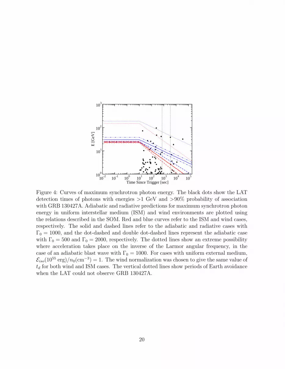
Figure 4: Curves of maximum synchrotron photon energy. The black dots show the LATdetection times of photons with energies >1 GeV and >90% probability of associationwith GRB 130427A. Adiabatic and radiative predictions for maximum synchrotron photonenergy in uniform interstellar medium (ISM) and wind environments are plotted usingthe relations described in the SOM. Red and blue curves refer to the ISM and wind cases,respectively. The solid and dashed lines refer to the adiabatic and radiative cases withΓ0 = 1000, and the dot-dashed and double dot-dashed lines represent the adiabatic casewith Γ0 = 500 and Γ0 = 2000, respectively. The dotted lines show an extreme possibilitywhere acceleration takes place on the inverse of the Larmor angular frequency, in thecase of an adiabatic blast wave with Γ0 = 1000. For cases with uniform external medium,Eiso(1055 erg)/n0(cm

−3) = 1. The wind normalization was chosen to give the same value oftd for both wind and ISM cases. The vertical dotted lines show periods of Earth avoidancewhen the LAT could not observe GRB 130427A.

20

Supplementary Materials

Systematics

The high flux during the brightest part of the burst saturated the GBM TTE data typefor all the GBM detectors, and as a result the TTE data from T0+4.9 s to T0+11.4 s wereunsuitable for analysis. The temporally binned CSPEC (1.024-s bins for 600 seconds aftera trigger, 128 energy channels) and CTIME (0.064-s bins for 600 seconds after a trigger,8 energy channels) data types were unaffected by saturation. However, due to the highevent rate, all data types were affected by pulse pileup during the brightest part of theburst, which significantly distorts the spectrum when the detector event rate surpasses∼80,000 counts per second. We excluded the data between T0+4.5 s and T0+11.5 s fromour spectral fits of the combined GBM and LAT emission.

Minimum variability analysis

The temporal variability of a GRB can give insight into the dynamics of the emissionregion, with direct implications for the opacity of the emitting region and, therefore,the bulk Lorentz factor. To study the variability of the γ-ray emission, we applied amodified version of the wavelet transform analysis presented in MacLachlan et al. 2013(38 ), where we used Maximum Overlap Discrete Wavelet Transform (MODWT) insteadof the Discrete Wavelet Transform (DWT). The former has superior statistical properties,especially in the context of the variance analysis (39 ). We applied this technique, whichdoes not require to assume a pulse shape, to the LLE >10 MeV data between T0 +3 andT0+20 s. The minimum variability time scale measured with this technique has previouslybeen shown to be a good proxy for the minimum rise time in GBM GRBs (40 ).

For GRB 130427A, we find an upper limit to the minimum variability timescale of0.04 ± 0.01 s, so that the shortest-duration significant features in the light curve havewidths of 0.08 ± 0.02 s. We double checked this result by using the Bayesian Blockalgorithm of Scargle (1998) (41 ), and again found time structures with a width of ∼0.08 sat the >5σ level. Given that the LLE light curve is brightest between T0+5 s and T0+15 s,it follows that the minimum variability time scale we calculated is most closely associatedwith this time interval. However, the minimum variability time scale is a measure of thetypical size of the emitting region, which is unlikely to change quickly within the promptemission.

Correlated variability analysis

We studied the temporal behavior of this GRB and searched for correlated variabilitybetween the keV and MeV-GeV emission, which, if present, would suggest that the low-and high-energy emission might arise from the same emission episode. We applied thediscrete correlation function method (42 ) to compare the global temporal behavior of low

21

and high energy emission, between T0−5 s and T0+20 s. For the first peak at T0 we foundthat the GBM emission lags the LLE emission, with an increasing lag with decreasingGBM energy; this is discussed in greater detail in the accompanying GBM paper on thisburst (43 ).

The saturation during the brightest part of this burst (T0 + 4.9 s to T0 + 11.4 s)prevented us from using TTE data, and as the analysis is very sensitive to bin size,the binned GBM data were not appropriate. We instead performed the analysis with theINTEGRAL/SPI-ACS light curve (∼80 keV – ∼10 MeV (44 ) and the LLE >10 MeV lightcurve. (The number of observed photons >100 MeV does not provide adequate statisticalpower to perform this kind of timing analysis on the LAT > 100 MeV data.) We foundsome indications that the correlation between the SPI-ACS and LLE emission decreaseswith increasing LLE energy, although this could be an effect of decreasing statistics.

Spectral analysis

In order to further explore the relation between the low- and high-energy emission, weperformed a time-resolved spectral analysis.

Production and availability of the spectra

We produced the spectra for LAT data by using the standard software package Fermi

ScienceTools (v9r31p1)1. LAT data above 100 MeV are available at the Fermi ScienceSupport Center2, while LLE and GBM data are available in the standard Browse interfaceof the HEASARC34.

The procedure to obtain the observed spectra, the background spectra and the re-sponses are described in details in (13 ).

In order to make it easier to reproduce our results we present the LAT spectra andresponses for all intervals for which we performed a spectral analysis in this paper (seeTable S2), and for the intervals used in (7 ). These files can be downloaded from ourpublic server5, and they can be loaded in XSPEC6.

Spectral modeling

For the higher-energy emission, we used the LLE >30 MeV events (the energy resolutionis poor between 10 and 30 MeV) and LAT >100 MeV Pass 7 Transient class events (1 ).For the GBM band, we used the TTE data between 8 keV and 900 keV from NaI detectors

1http://fermi.gsfc.nasa.gov/ssc/2http://fermi.gsfc.nasa.gov/ssc/data/3http://heasarc.gsfc.nasa.gov/W3Browse/fermi/fermille.html4http://heasarc.gsfc.nasa.gov/W3Browse/fermi/fermigbrst.html5https://www-glast.stanford.edu/pub data/6https://heasarc.gsfc.nasa.gov/xanadu/xspec

22

6, 9, and 10 (which had the smallest source angles and therefore the best exposures to thesource), and the corresponding BGO detector 1 (which is positioned on the same side ofthe spacecraft as NaI detectors 6, 9, and 10). For the NaI detectors, we excluded the datafrom the energy bins near the K-edge (16 ). The spectral fits were performed using bothRMFIT (version 4.3BA) and XSPEC (version 12.8), with consistent results. We reporthere the fits obtained with RMFIT by minimizing the Castor statistic (CSTAT), whichmodifies the Cash statistic for Poisson distributed data by a data-dependent quantity sothat the statistic asymptotes to χ2 as the number of counts becomes large7.

The models we considered were a power law (“PL”), a Band function (“Band”), anda smoothly broken power law (“SBPL”). The PL model has the form

fPL(E) = A

(

E

Epiv

)λ

,

where A is the normalization (in photons cm−2 s−1 keV−1) and Epiv, the pivot energy(which normalizes the model to the energy range being studied), is fixed to 100 keV. Inour analyses, the PL model was only used as an extra component.

The Band function is an SBPL whose curvature is defined by the spectral indices (15 ).It has the form

fBand(E) =

A(

EEpiv

)α

exp[

− (α+2)EEpeak

]

, E ≤ α−β2+α

Epeak

A(

EEpiv

)β

exp(β − α)[

α−β2+α

Epeak

Epiv

]α−β

, E > α−β2+α

Epeak

where α and β are the low- and high-energy indices, respectively, and Epeak is the energyat which the νFν spectrum reaches a maximum. We set Epiv = 100 keV.

We also used the more general SBPL model, parameterized as

fSBPL(E) = A

(

E

Epiv

)b

10(a−apiv), where

a = m∆ ln

(

eq + e−q

2

)

, apiv = m∆ ln

(

eqpiv + e−qpiv

2

)

,

q =log(E/Eb)

∆, qpiv =

log(Epiv/Eb)

∆,

m =λ2 − λ1

2, b =

λ2 + λ1

2,

where Eb is the break energy (in keV), λ1 and λ2 are the low- and high-energy indices,respectively, and ∆ is the break scale (in decades of energy) (16 ).

7https://heasarc.gsfc.nasa.gov/xanadu/xspec/manual/XSappendixStatistics.html

23

Temporally extended emission

For the analysis of photons with energies >100 MeV arriving before the first occultation(T0 + 710 s), we used the Transient class event selection selecting events within a 12-radius region of interest (ROI) centered on the burst location. This region of interestwas reduced to 8 for the last interval before the Earth occultation in order to reducebackground contamination by γ rays from the Earth’s limb produced by interactions ofcosmic rays with the upper atmosphere. After the first occultation we used the Source

class event selection, which has more stringent background rejection cuts than Transient

class events and is better suited for analyses of long time intervals and dimmer sources.We adopted also a smaller 10-radius ROI, which reflects the better PSF of the Source

class.We used an unbinned maximum likelihood analysis to model the high-energy emission

from the GRB. This was done with the standard software package Fermi ScienceTools(v9r31p1)8, and in particular the Python Likelihood analysis9. The GRB was modeled asa point source at the best available position of the afterglow (45 ). For every time intervalshown in Figure 2 in the main text, we tried both a power-law and a broken power-lawmodel for the spectrum of the source, but we found no statistically significant evidencefor a break. We also tried larger time intervals, and did not find significant improvementsby using the broken power law instead of a simple power law. Therefore, contrary to Tamet al. (18 ), we conclude that there is no statistically significant evidence for a break inthe LAT energy spectrum. Instead, we explain the excess at high energy seen by Tam etal. as an effect of spectral evolution (see next section). We therefore used a power law tomodel the spectrum of the source.

An isotropic background component is included in the fit. For the analysis withTransient class, the spectral properties of the isotropic component are derived using anempirical background model (46 ) that is a function of the position of the source in the skyand the position and orientation of the spacecraft in orbit. For the analysis with Source

class, instead, we used the publicy available Isotropic template10. These backgroundmodels accounts for contributions from both residual charged particle backgrounds andthe time-averaged celestial γ-ray emission. Their normalizations are kept free during thefit. A Galactic component, based on the publicy available model for the interstellar diffuseγ-ray emission from the Milky Way, is also included in the fit, with a fixed normalization.For all time intervals, we also included all the 2FGL sources within the ROI (47 ).

We usually use Source class events for analyses of time intervals longer than 100 s.However, for GRB 130427A, the signal-to-noise was in Transient than Source class pho-tons up until the first Earth occultation. We obtained consistent results with Source classevents, although the statistical uncertainties were larger.

8http://fermi.gsfc.nasa.gov/ssc/9http://fermi.gsfc.nasa.gov/ssc/data/analysis/scitools/python tutorial.html

10http://fermi.gsfc.nasa.gov/ssc/data/access/lat/BackgroundModels.html

24

Spectral Energy Distributions

We evaluated the spectral energy distribution (SED) from the LAT data for several dif-ferent time intervals, using the following procedure: In each time bin, we first performedan unbinned maximum likelihood analysis selecting the full energy range (100 MeV to100 GeV) using Pass7 v6 Source class photons. We selected events within 10 from thelocation of GRB 130427A. The diffuse Galactic background component normalization wasfixed, while the normalization of the isotropic background component was left free. Wemodeled GRB 130427A as a point source with either a spectrum described by a simplepower law with normalization and index free or a spectrum described by a broken powerlaws. We recorded the value of the normalization of the isotropic component for the bestfit model.

Then, we selected events for six energy ranges (100 MeV–237 MeV, 237 MeV–562MeV, 562 MeV–1.3 GeV, 1.3 GeV–3.2 GeV, 3.2 GeV–11.6 GeV, 11.6 GeV–100 GeV) andwe independently performed a likelihood analysis in each energy bin, fixing the isotropicbackground component normalization to the value previously obtained. The normaliza-tion and the photon index of the GRB source were left free. We calculated the SED pointsby multiplying the integrated flux in each energy bin by the square of the average energycalculated using the best-fit power-law index. We report our results in Figure S1, wherethe vertical bar position coincides with the estimated average energy. The choice of thetime bins was driven by features in the LAT light curve of Figure 2 (intervals a, b, andd) and the choice in (18 ) (intervals c, e).

We compared our results with Tam et al. (18 ), and we found that in all the timeintervals, the simple power-law model better describes the data well, and the broken powerlaw is not statistically required. Also, we notice that the SED in interval d is consistentwith the sum of the hard component spectrum of interval b and the soft componentspectrum in interval a and c. This points to the spectral evolution as source of the high-energy excess, rather than the simultaneous co-existence of two components, as claimedby (18 ).

Constraints on Γ

A minimum bulk Lorentz factor Γmin for GRB 130427A can be calculated by using thevariability timescale tvar, obtained as described above, to estimate the size scale ∆r′ ∼=Γctvar/(1 + z) of the emission region. The comoving photon energy density u′(ν ′) in thefluid frame is related to the measured spectral luminosity through the expression νLν =4πd2LΓ

2u′(ν ′), where ν ′ ∼= ν/Γ (for details, see SOM in (48 )). The value for Γmin∼= 500

is derived for the 73 GeV photon detected at 19.06 s after T0, as described in the text.This uses a value of tvar determined from the LLE light curve (see Minimum VariabilityAnalysis). The uncertainties in Γmin quoted in the text are formal uncertainties, relatedto the uncertainty in tvar , and do not include the uncertainties related to the errors in the

25

102 103 104 105

Energy [MeV]

10-6

10-5

a) 138-196 s

102 103 104 105

Energy [MeV]

10-6

10-5

b) 196-257 s

102 103 104 105

Energy [MeV]

10-6

10-5

E2 dN/dE [erg cm−2]

c) 257-750 s

102 103 104 105

Energy [MeV]

10-6

10-5

d) 138-750 s

102 103 104 105

Energy [MeV]

10-6

10-5

e) 3000-80000 s

Figure S1. Spectral Energy Distribution of LAT data in five different time intervals(a=138–196 s, b=196–257 s, c=257–750s, d=138–750 s, e= 3000s–80000 s).

26

best fit parameters and photon statistics, the latter giving ∼ 20% uncertainty of Γmin.The initial bulk Lorentz factor Γ0 can be determined by assuming that the duration

of the brightest LAT emission corresponds to the deceleration timescale td. For a uniformcircumburst medium with density n = n0(cm

−3), td = (3Eiso/4πΓ80nmpc

2)1/3/c ≡ 10t1 s,implying Γ0

∼= 540(E55/nt31)1/8, where Eiso ≡ 1055E55 erg, which is larger than Eγ,iso bya factor of ≈ 7. Relations for determining Γmin in a medium with a power-law densitygradient can be found in (49 ).

Maximum synchrotron energy

In the coasting and deceleration phases, the evolution of Γ with radius r for an adiabaticblast wave in a uniform circumburst medium (the ISM case) can be parameterized bythe function Γ(r) ∼= Γ0/

√

1 + (r/rd)3. Generalization to different radiative regimes andcircumburst density gradients can be made through the expression

Γ(r) =Γ0

√

1 + aqxq≡ Γ0Gq(x) , x ≡ r

rd, (1)

where rd = (3Eiso/4πnmpc2Γ2

0)1/3. By choosing q and aq appropriately, these parame-

terizations recover the exact asymptotes in the deceleration phase. For the adiabaticBlandford-McKee (1976) solution in the ISM case, q = 3 and a3 = 0.70, which is ob-tained from the expression r = (17E〉∫ ≀/16πΓ2nmpc

2)1/3 (24, 50 ). Alternately, one cantake aq = 1 and define rd such that Γ(r) recovers the self-similar solution.

The maximum synchrotron photon energy in the stationary frame of the black holeis ǫmax,syn = δDǫ

′cl (in units of mec

2), where the Doppler factor δD = [Γ(1 − βµ)]−1 →2Γ/(1 + Γ2θ2) in the limit Γ(r) ≫ 1 and θ ≪ 1. Equating the inverse of the timescaleto execute a complete Larmor orbit with the timescale for synchrotron losses gives theclassical, radiation-reaction limited value of ǫ′cl = 27/16παf

∼= 74 ∼= 38/0.511, whereαf = 1/137 is the fine-structure constant. A more stringent but less physically plausi-ble criterion equates the synchrotron timescale with the inverse of the Larmor angularfrequency, which will allow ǫ′cl to be a factor of 2π larger.

The time t∗ in the stationary frame relates to the time t in the observer frame foremission at radius r and angle θ = cos−1 µ to the line of sight through the expressiont = t∗ − rµ/c. Taking r as the radius of the forward shock, dr = βshcdt∗ = βshΓshcdt

′ =βshδD,shΓshcdt, so that

dt =dr

βshΓshδD,shc→ dr

2Γ2shc

(1 + Γ2shθ

2) ∼= dr

4Γ2c(1 + 2Γ2θ2) (2)

in the limit Γ ≫ 1 and θ ≪ 1, where the shocked fluid Lorentz factor Γ ∼= Γsh/√2 ≫ 1.

This differential equation can be rewritten in terms of rd and td = rd/2Γ20c using the

variables τ = t/td, and N = Γ0θ, giving 2dτ = dx(1 + 2N2 + aqxq), with solution

27

τ = [(1 + 2N2)x + aqxq+1/(q + 1)]/2. This expression was numerically inverted to give

x(τ, N). The maximum synchrotron photon energy ǫmax,syn at time t = tdτ is found bynumerically scanning through N = Γ0θ in the expression

ǫ(τ, N) =2Γ0Gq[x(τ, N)]ǫ′cl1 +N2G2

q[x(τ, N)](3)

to find its maximum value.When tdec > td, that is, when the engine duration TGRB > td, the above computation is

modified somewhat. When t > tdec, the computation is the same as for the case td < TGRB .When t < tdec, we let Γ(t) → Γ0(tdec), where Γ0(tdec) = (2ctdec)

−3/8(3Eiso/4πnmpc2)1/8 ∼=

1280[tdec(s)]−3/8(E55/n)1/8. Note, however, that even for TGRB < td = tdec, the shell

spreads radially and the reverse shock becomes mildly relativistic at t ∼ tdec. ThusΓ(tdec), representing the bulk Lorentz factor of the newly shocked material around thattime, could be a factor ≈ 2 lower than given by this expression. Here we use the moreoptimistic expression for Esyn,max.

Figure S2 shows results for an adiabatic blast wave in the ISM case with Γ0 = 500and 1000, and TGRB = 1 and 100 s, for z = 0.34 and E55/n0 = 1. The cases withTGRB = 1 and 100 s are illustrative, showing the effects of injection when TGRB < tdec(the impulsive regime), and when TGRB > tdec (the extended-engine regime). We useTGRB = 10 s when comparing with data from GRB 130427A, as this value correspondsto the timescale during which most of the energy is emitted, as shown by the GBM lightcurves. Note that Nmax is nonzero during the coasting phase when TGRB > td.

The curves, as labeled, show the on-axis values of Γ(t, N = 0), the off-axis values ofΓ(t, N = Nmax) that produce the highest energy synchrotron photons. Also shown arethe on-axis and off-axis values of Emax,syn. These values are nearly identical because thelarger Lorentz factors of the off-axis emission compete with reduction of Doppler boostingwhen the emitting plasma is moving at an angle to the line of sight. The angle wherethe highest energy synchrotron photon originates, in units of 1/Γ0, is shown by the longdashed curve. The results of Figure S2 agree with Eq. (4) of (25 ), scaled by the factor27/16π.

28

0

5

10

15

20

Nm

ax

10-1

100

101

102

103

104

time [sec]

100

101

102

103

10-1

100

101

102

103

104

time [sec]

0

5

10

15

20

Nm

ax

100

101

102

103

10-1

100

101

102

103

104

time [sec]10

-110

010

110

210

310

4

time [sec]

Γ(t)

Emax

[GeV]

td = 12 sec

TGRB

= 100 sec

E55

/n0 = 1

Γ0 = 500

td = 12 sec

TGRB

= 1 sec

E55

/n0 = 1

Γ0 = 500

td = 1.9 sec

TGRB

= 1 sec

E55

/n0 = 1

Γ0 = 10

3

td = 1.9 sec

TGRB

= 100 sec

E55

/n0 = 1

Γ0 = 10

3

Figure S2. Adiabatic evolution of the bulk Lorentz factor Γ with time t in a uniformcircumburst medium, showing the on-axis bulk Lorentz factor Γ(t, N = 0) (solid bluecurves), and the value of Γ(t, Nmax) that produces the most energetic synchrotron photonenergy at time t (dotted blue curves), where N ≡ Γ0θ and Nmax = Γ0θmax. In all cases,E55/n0 = 1. The maximum synchrotron photon energy from on-axis emission is givenby the solid red curves, and from off-axis emission by the dashed red curves. At earlytimes, the two are equal, and given by 2

√2× 38 MeV ×Γ0/1.34 ∼= 40 GeV for Γ0 = 500,

TGRB ≪ tdec. The green dot-dashed curve gives the value of Nmax that maximizes themaximum synchrotron photon energy. (a) Top left: Γ0 = 500, TGRB = 1 s. (b) Top right:Γ0 = 500, TGRB = 100s. (c) Bottom left: Γ0 = 1000, TGRB = 1 s. (d) Bottom right: Γ0

= 1000, TGRB = 100 s.

29

Time interval Model Norm. Ebreak ∆ λ1 λ2 C-STAT / dof

(a) -0.1 to SBPL 0.3145 ± 0.0015 291 ± 23 1.08 -0.334 ± 0.025 -3.394 ± 0.072 700 / 4744.5 s

(b) 4.5 to PL 189 ± 165 – – -3.34 ± 0.15 – 20 / 1511.5 s

(c) 11.5 to SBPL 0.1000 ± 0.0003 39.1 ± 3.3 1.11 -0.623 ± 0.050 -2.408 ± 0.012 1028 / 47433.0 s

SBPL 0.1003 ± 0.0005 60.0 ± 7.8 1.11 -0.784 ± 0.046 -2.515 ± 0.037 984 / 472

+PL (4.2+6.0

−3.0) × 10−4 – – -1.66 ± 0.13 –

(d) 33.0 to SBPL 0.0133 ± 0.0001 7.3 ± 3.2 1.21 0.37 ± 0.59 -2.238 ± 0.012 406 / 241196.0 s

SBPL 0.0133 ± 0.0001 7.3 ± 3.6 1.21 0.41 ± 0.65 -2.247 ± 0.020 401 / 239

+PL (1.6+2.8

−1.0) × 10−6 – – -1.22 ± 0.68 –

Table S1. The prompt emission spectral fit parameters, using GBM, LLE, an LAT data(except for interval b, which only uses LLE and LAT data). All times are relative toT0. We tried to fit a smoothly broken power law (“SBPL”) as well as an SBPL with anextra power-law (“PL”) component. Parameters are: normalization in photons cm−2 s−1

keV−1, Ebreak in keV, break scale ∆ (for SBPL) in decades of energy, low-energy indexλ1, and high-energy index λ2. C-STAT is the Castor statistic (a modified version of theCash statistic). See text for definitions of models. For all time intervals that were fit witha SBPL, we fixed the break scale ∆ to the best-fit value. The extra PL component isstatistically significant in interval c (∆CSTAT = 44 for 2 degrees of freedom). In intervald, we used only NaI detector 6.

E Erf T − T0

95 128 243.5573 97 19.0647 63 256.7041 55 611.0139 52 3410.2632 43 34366.5828 37 48.0126 35 85.1621 21 141.5315 20 217.89

Table S2. The 10 highest-energy LAT photons with probability >1− 10−3 of being asso-ciated with the GRB as opposed to background, determined using a likelihood analysis.Erf is the photon’s rest frame energy at the redshift z = 0.34. All photons are Source

class. E and Erf are in GeV, T − T0 in s.

30