Embed Size (px)
Citation preview
Fermi National Accelerator Laboratory FERMILAB-Pub-79/17-THY
Asymptotic Freedom in Deep Inelastic Pgocesses in the Leading Order and Beyond
ANDRZEJ 3. BURAS Fermi National Accelerator Laboratory
P.O. Box 500, Batavia, Illinois 60510 USA
ABSTRACT
The present status of Quantum Chromodynamics formalism for inclusive
deep-inelastic scattering is reviewed. Leading order and higher order asymptotic
freedom corrections are discussed in detail. Both the formal language of operator
product expansion and renormalization group, and the intuitive parton model
picture are used. Systematic comparison of asymptotic freedom predictions with
deep-inelastic data is presented. Extensions of asymptotic freedom ideas to other
processes such as massive u -pair production, semi-inclusive deep-inelastic scat-
tering, e’e- annihilation and photon-photon scattering are briefly discussed. The
importance of higher order corrections is emphasized.
*Based on the lectures given by the author at the VIth International Workshop on Weak Interactions, Iowa, 1978, and the academic training lectures presented at Fermilab, February, 1979.
a Operated by Universities Research Association inc. under contract with the Energy Research and Development Administration
i
Contents
FERMILAB-Pub-79/17-THY
P 1. Introduction
A. Preliminary Remarks
8. Out1 ine
II. Parton Model and Asymptotic Freedom Formulae
A. Preliminaries
1. Deep inelastic structure functions
2. Bjorken scaling and its intuitive interpretation
B. Basic Formulae of the Parton Model
1. Parton distributions
2. Electromagnetic structure functions
3. v and 7 cross-sections
4. v and v structure functions
5. Basic properties of the simple parton model
6. Beyond the simple parton model
c. Basic Formulae of Asymptotic Freedom
1. Leading order
1.1. Effective coupling constant
1.2. Intuitive approach
1.3. Formal approach
1.4. Marriage of the intuitive and the formal approach
2. Higher order corrections
2.1. Effective coupling constant
2.2. Non-singlet structure functions
2.3. Corrections to parton model sum rules
1
1
2
6
6
6
7
9
9
11
11
14
1.5
17
18
18
19
20
23
29
31
31
32
34
ii FERMILAB-Pub-79/17-THY
2.4. Singlet structure functions 35
2.5. Miscellaneous remarks 39
D. [Mass Corrections 40
1. Target mass corrections 41
2. Heavy quark mass corrections 44
E. Structure of Common Asymptotic Freedom Phenomenoiogy 45
1. Leading order 45
2. Higher orders 47
F. Parton Model Formulae for Higher Order Corrections Longitudinal Structure Functions
III. &antum Chromodynamics and Tools to Study it
48
53’
A. Lagrangian and Feynman Rules 53
B. Renormalization and Renormalization Group Equations 55
1. Dimensional regularization 55
2. Renormalization 57
3. Two subtraction schemes 59
3.1. Subtraction at p2 q p2 59
3.2. ‘t Hooft’s minimal subtraction scheme 60
4. Renormalization group equations 62
5. Calculations of renormalization group functions 65
C. Operator Product Expansion 68
D. Renormalization Group Equations for Wilson Coefficient Functions 72
E. Calculations of Anomalous Dimensions of Local Operators
IV. Q2 Dependence of the Moments of Structure Functions in Asymptotically Free Gauge Theories
A. Preliminaries
7.5
80
80
B. Non-singlet Structure Functions 82
c. Singlet Structure Functions 85
. . . 111 FERMILAB-Pub-79/17-THY
V. Q2 Dependence of Parton Distributions in the Leading Order
A. Intuitive Picture and Integro-differential Equations
B. Asymptotic Freedom Equations for the Moments of Parton Distributions
C. Equivalence of the Intuitive and the Formal Approach
D. Properties of Parton Distributions
E. Approximate Solutions of Asymptotic Freedom Equations
VI. Short Review of Asymptotic Freedom Phenomenology
A. Electroproduction and Muon Scattering
1. Structure functions
2. Moment analysis
B. v and 7 Deep-Inelastic Scattering (Charged Currents)
1. Total cross-sections
2. <Y’
3. a>, <xy>, <x” >
4. IdxFi(x, E) and Jdx x”Fi(x, Eh)
5. x distributions
6. v and 3 structure functions
7. Moment analyses of BEBC and CDHS
8. Comments on neutral current processes
c. Comments on Fixed Point Theories
D. Critical Summary
VII. Higher Order Asymptotic Freedom Corrections to Deep-Inelastic Scattering (Non-singlet Case)
A. Preliminaries
92
92
97
99
102
107
111
111
111
‘113
113
113
115
115
116
118
119
119
123
123
127
127
127 -3
B. Wilson Coefficient Functions of Non-singlet Operators to Order g” 130
c. Procedure for the Calculation of BiSn 136 9 D. Renormalization Prescription Independence of Higher Order
Corrections 138
iv FERMILAB-Pub-79/17-THY
E. Results for y $“” and Bysn . I
1. (l),n Two-loop anomalous dimensions y NS
2. Bisn in 9 Hooft’s scheme (electromagnetic currents)
3. B& k n in ‘t Hooft’s scheme (weak CUtTentS) 9
4. Corrections to sum rules and parton model relations
F. Phenomenology of the Order jj2 Corrections (Non-singlet Case)
G. An Schemes
H. Other Definitions of E2(Q2)
VIII. Higher Order Asymptotic Freedom Corrections to Deep-Inelastic Scattering ( Singlet Case)
A. Preliminaries
B. Moments of the Singlet Structure Functions
c. A(l),n $ Results for y G ’ Bk,n and Bk,n
1. Two-loop anomalous dimension matrix
2. Bt n and Bt n in 9 Hooft’s scheme 9 9
IX.
3. Comparison of various calculations
4. Discussion of the In 41t - y E terms
D. Numerical Estimates
E. Parton Model and Higher Order Corrections
F. More about Callan-Gross Relation
Asymptotic Freedom Beyond Deep Inelastic Scattering
A. Preliminaries
B. Factorization and Perturbative QCD
C. Lessons from Deep-inelastic Scattering
D. e+e- -f hadrons
E. Photon-Photon Collisions
F. Semi-inclusive Processes in QCD
141
141
142
143
145
146
151
155
157
157
157
168
168
169
173
175
176
178
183
187
187
190
191
192
195
201
FERJJILAB-Pub-79/17-THY
1. Preliminaries 201
2. Fragmentation Functions 203
3. Drell-Yan and semi-inclusive deep-inelastic scattering 211
G. Miscellaneous remarks 216
X. Summary 218
Acknowledgments
Appendix A: Basic Formulae of the Dimensional Regularization
Appendix B: Parton Distributions and ‘Matrix Elements of Local Operators. Charge Factors.
Footnotes
References
Tab1 es
Figure Captions
Figures
220
221
224
226
232
246
251
-l-
I. INTRODUCTION
FERMILAB-Pub-79/17-THY
A. Preliminary Remarks
Quantum Chromodynamics (QCD) is the most promising candidate for a
theory of strong interactions. It has the property of asymptotic freedom which
seems to be consistent with the deep inelastic data, and it provides a possibility of
confining quarks and gluons. The quark and gluon confinement in QCD has not yet
been proven. On the other hand, the theoretical structure of asymptotic freedom
in deep inelastic scattering, in the leading order and in the next to the leading
order in the effective strong interaction quark-gluon coupiing constant, seems to be
well understood by now. Also a great effort has been made in comparing
asymptotic freedom predictions with the experimental data. We think it is an
appropriate time to review the present situation.
The progress in understanding the structure of asymptotic freedom in deep-
inelastic scattering proceeded in several steps during the last six years. Just after
the discovery of asymptotic freedom (Gross and Wilczek, 1973a, b; Politzer, 1973),F’
all calculations relevant for the leading behavior of the moments of the deep-
inelastic structure function were performed (Georgi and Politzer, 1974; Gross and
Wilczek, 1974; Bailin, Love and Nanopoulos, 1974). Three years later these results
were put in a form useful for phenomenological applications (de Rujula, Georgi and
Politzer, 1974; Altarelli, Parisi and Petronzio, 1976; Glcck and Reya, 1977a,b;
Buras 1977; Buras and Gaemers, 1978; Hinchliffe and Llewellyn-Smith, 1977a;
Altarelli and Parisi, 1977; Tung, 1975, 1978; Fox, 1977)!%ntil recently almost all
asymptotic freedom phenomenology has been based on the leading order formulae.
During the last two years, the structure of the higher order asymptotic freedom
corrections to deep-inelastic scattering has been finally understood and completed
(Zee, Wilczek and Treiman, 1974; Caswell, 1974; Jones, 1974; Floratos, Ross and
-2- FERMILAB-Pub-79/17-THY
Sachrajda, 1977, 1979; Bardeen, Buras, Duke and Muta, 1978; Altarelli, Ellis,
Martinelli, 1978) and some phenomenological applicarions of these higher order
results have been made.
Parallel 10 the development in deep-inelastic scattering there has been a lot
of progress in the extension of asymptotic freedom ideas to other than deep-
inelastic processes and it is appropriate to present in this review some of the
results of these studies.
B. Outline
The main purpose of this review is to present
(i) the leading order of asymptotic freedom and its phenomenological
implications together with comparison with deep-inelastic data,
(ii) the structure of higher order asymptotic freedom corrections and their
effect on leading order results.
We shall also briefly discuss
(iii) leading order and higher order asymptotic freedom corrections to other
than deep-inelastic processes.
This review is organized in a rather unconventional way, which we shall try
to justify below. Section II will be what one could call a handbook of parton model
and asymptotic freedom formulae relevant for deep-inelastic scattering. We begin
this Section by recalling basic ideas behind the simple Parton Model with Bjorken
scaling and we quote some of its well-known formulae which will be useful in the
subsequent sections. We then present systematically all asymptotic freedom
expressions (leading and next to the leading order) necessary for the study of the
scaling violations in deep-inelastic scattering. This section ends with a general
structure of present day asymptotic freedom phenomenology in the form of a
procedure. This hopefully will enable anybody to make her (his) own QCD fit to
deep-inelastic data. One might think that it is a bad idea to begin a review with a
-3- FERMILAB-Pub-79/17-THY
vast array of formulae. In the standard reviews, one usually relegates them to an
appendix or to the last section of the text. We think, however, that such an
exposition of the formulae and of the general structure of asymptotic freedom at
the beginning will give the reader a good feeling about the whole subject and
hopefully will enable her (him) to begin her (his) own research in this field without
reading too much.
The derivations, discussions, explanations and intuitive interpretations of the
formulae of Section II are contained in the main part of the review, namely in
Sections III to VIII. Section III deals with QCD as the field theory of colored quarks
and gluons. The basic tools necessary to study QCD implications for deep-inelastic
scattering are systematically presented here. After recalling the Feynman rules
for QCD, we discuss briefly the concepts of regularization and renormalization. In
particular we illustrate with examples dimensional regularization (‘t Hooft and
Veltman, 1972) and the minimal subtraction scheme (‘t Hooft, 1973). Subsequently
we discuss renormalization group equations in general. Next we present the
operator product expansion and its relation to the moments of deep-inelastic
structure functions. Finally we derive renormalization group equations for the
Wilson coefficient functions and show with examples how to calculate anomalous
dimensions. This Section may be omitted by experts and pedestrian readers,
without loss of continuity.
In Section IV we present the formal approach to deep-inelastic scattering
based on the operator product expansion and renormalization group. We deal here
explicitly with the mixing of gluon and singlet fermion operators. The main result
of this section is an expression for the moments of an arbitrary structure function
in terms of the Wilson coefficient functions with an explicit Q2 dependence
calculated in the leading order.
-4- FERMILAB-Pub-79/17-THY
In Section V we turn to a more intuitive approach to asymptotic freedom
which, on the one hand, is a simple extension of parton model ideas and, on the
other hand, is equivalent to the formal approach developed in Section IV. The main
results of this section are the equations for the Q2 dependence of effective parton
distributions. We discuss various properties of these equations and give their
approximate analytic solutions.
In Section VI we list various implications of asymptotic freedom for deep-
ineiastic processes. Subsequently, we confront these predictions with the recent
high energy ep, pp, vN and TN data.
In Section VII we discuss asymptotic freedom beyond the leading order. This
section is rather formal, We discuss first the non-singlet case because it is simpler
than the singlet one. The renormalization dependence and independence of various
quantities is dealt with in some detail. Also a discussion of the meaning of the
parameter A, the sole scale parameter of the theory (except for masses), is given.
Corrections to various parton model sum rules and relations are presented. After a
phenomenological application of non-singlet formulae we turn in Section VIII to the
singlet case which we present in detail. We discuss some phenomenological
implications of the singlet formulae for deep-inelastic data. We also present
parton model formulae for these higher order corrections. We end Section VIII by
discussing longitudinal structure functions.
In Section IX we discuss briefly the extension of asymptotic freedom ideas to
other processes such as massive u-pair production, semi-inclusive deep-inelastic
scattering, e+e- annihilation and photon-photon scattering.
Finally in Section X we make a few concluding remarks. The paper ends with
two Appendices where the basic formulae of the dimensional regularization and the
relations between parton distributions and the matrix elements of local operators
are given.
-5- FERMILAB-Pub-79/ 17-THY
In the last six years there have been many very good reviews on asymptotic
freedom (e.g. Politzer, 1974; Gross, 1976; Ellis, 1976; Gaillard, 1977; Altarelli,
1978a;Nachtmann, 1977; LIewell yn-Smith, 1978a, Ross, 1979 f3 The new topic
discussed here, which has not been presented in the reviews above (except for some
discussion in the review by Ross), are the higher order corrections (Sections VII,
VIII). We have also attempted to present the whole material in a form easy for
phenomenological applications. While completing this review we received a very
nice review article by (Peterman, 1979) who also discusses, among other topics,
higher order asymptotic freedom corrections in some detail. Although unavoidably
there is some overlap between Peterman’s and our review, the structure and
presentation of both reviews is quite different.
-6- FERMILAB-Pub-79/17-THY
II. PART-ON MODEL AND ASYMPTOTIC FREEDOM FORMULAE
A. Preliminaries
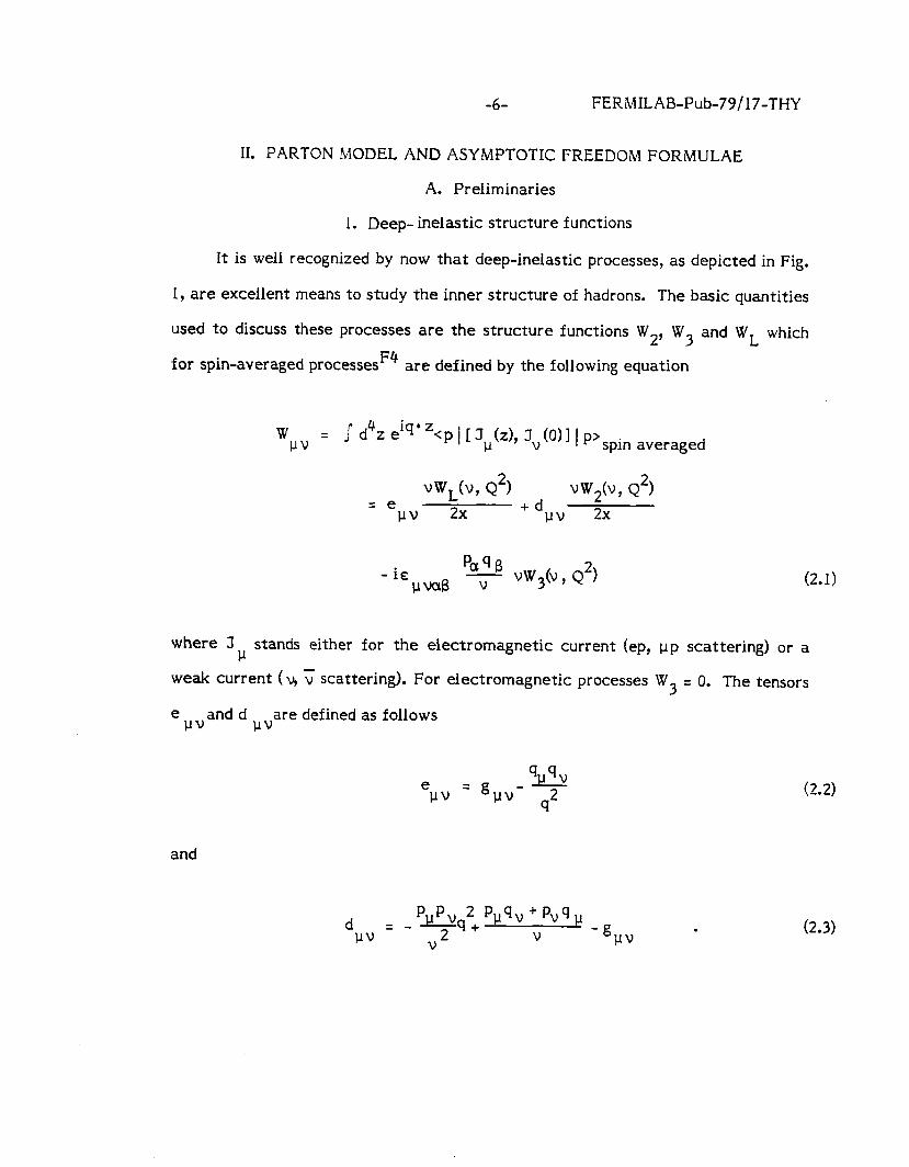
1. Deep- inelastic structure fUnCtiOnS
It is well recognized by now that deep-inelastic processes, as depicted in Fig.
1, are excellent means to study the inner structure of hadrons. The basic quantities
used to discuss these processes are the structure functions W 2, W3 and WL which
for spin-averaged processes F4 are defined by the following equation
W PV
= I d4z eiqaz ‘P I [ Jp’Z)~ Jv to)] 1 P’spin averaged
= e vWL(v, Q2)
+d uW2b, 4’)
pv 2x pv 2x
- ie %%3 pm3 v vW3b, 4') (2.1)
where J P stands either for the electromagnetic current (ep, pp scattering) or a
weak current (v, u scattering). For electromagnetic processes W3 = 0. The tensors
e lJV
and d PV
are defined as follows
e q,qV
PV = gpv- q2
and
d plpvq2+ ppqv + pvq p j.lv=- v2 V -gpv l
(2.2)
(2.3)
-7- FERMILAB-Pub-79/17-THY
Kinematical variables are defined in Fig. 1. For the purpose of subsequent
sections, we prefer to deal with the longitudinal structure function VW L rather
than with WI. vWL and WI are related to each other as follows
VWL = VW2 -2xw1 . (2.4)
The dependence of the structure functions on the variables I, and Q2 is dictated by
the underlying theory of strong interactions. The main object of this review is to
study WL, W2 and W3 in the framework of Asymptotically Free Gauge Theories
(Politzer, 1973, 1974; G ross and Wilczek, 1973a, b)F5First, however, let us recall
how the structure functions in question behave in a simple parton model.
2. Bjorken scaling and its intuitive interpretation
As we indicated in Eq. (2.11, the structure functions depend generally on both
v and Q2. However, if v and Q2 are sufficiently large so that all mass scales can
be neglected, the dimensionless structure functions vW2, vW3, Wl and v WL will
depend only on
x=g i.e., we shall have Bjorken scaling (Bjorken, 1969 )
(2.5)
(2.6)
(2.7) Wi; + F;(x)
-8- FERMILAB-Pub-79/17-THY
Here i stands for a process considered i = UN, YN, ep, up, etc. The simple parton
model was introduced by (Feynman, 1969) as an intuitive picture of Bjorken scaling
wherein
i) target mass effects
ii) quark mass effects
iii) interactions between quarks (partons)
iv) <p12 > of partons and other possible scales
are neglected. This beautiful model is so well known to experimentalists and
theorists that there is no need to describe it here in detail. A few comments and a
collection of the most important parton model formulae are, however, necessary.
In the parton model one imagines that a photon, W-boson or 2’ scatters off a
free, pointlike constituent-parton (qi) as shown in Fig. 2a. The corresponding
virtual Compton amplitude is presented in Fig. 2b. In this picture, x is the fraction
of the proton momentum carried by the parton qi. On a more quantitative level
(Bjorken and Paschos, 1969, 1970; Kuti and Weisskopf, 1971; Feynman, 1972) one
introduces parton distributions (quark, antiquark) qi(x) and ti(x) which measure the
probability for finding a parton of type i in a proton with the momentum fraction x,
Then for instance
F;p(x) = 1 e; X [qi(x) + ii(‘) I i
(2.8)
.th where ei stands for the charge aof the 1 parton.
Similarly all deep-inelastic structure functions and various relevant cross-
sections can be expressed in terms of parton distributions weighted by the
appropriate electromagnetic or “weak” charges. In the following we shall recall the
rules for construction of these parton model formulae and subsequently list the
most important expressions.
-9- FEXVILAB-Pub-79/17-THY
8. Basic Formulae of the Parton Model
1. Parton distributions
In a four quark model (u, d, s, c) (Glashow, Iliopoulos and Maiani, 1970) we
decompose the proton into valence part
V(x) = u,(x) + d$) 9 (2.9)
the non-charmed sea
S(x) z u,(x) + ds (x) + c(x) + a(x) + s(x) + x(x) 9 (2.10)
the charmed sea
C(x) G c(x) + 3x1 9 (2.11)
and we introduce a gluon distribution G(x). The u(x) and d(x) distributions are then
given as foliows
u(x) = uv(x) + us(x) (2.12)
and
d(x) = dv(x) + d,(x) l (2.13)
-lO- FERMILAB-Pub-79/17-THY
In what follows it will be convenient to denote generally any quark and anti-
.th quark distribution corresponding to the 1 flavor, by qi(X) and qi(X), respectively,
and introduce the following combinations
and
Notice that
qtx) = r, qit’) I
(2.14)
~tx) = C 4itx) i
(2.15)
c(x) = q(x) + ?j(x) = v(x) + S(x) + C(x) (2.16)
qjcx) = qi(X) - qj(x) .
(2.17)
(2.18)
V(x) = q(x) - q(x) . (2.19)
The distributions Aij(x), pj(x) and V(x) are non-singlets under flavor symmetry
SU(4), whereas C(x) and C(x) are singlets. The distinction between non-singlet and
singlet distributions will be very important when we come to discuss asymptotic
freedom effects.
-ll- FERMILAB-Pub-79 / 17-THY
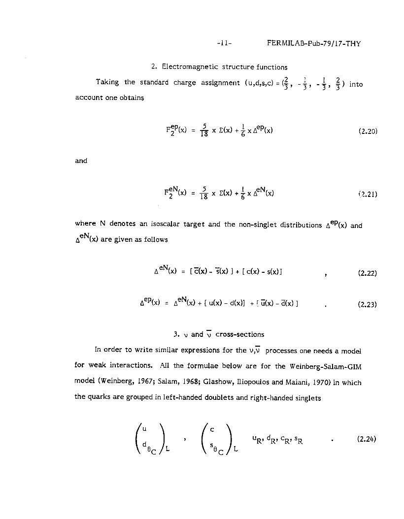
2. Electromagnetic structure functions
Taking the standard charge assignment (u,d,s,c) = ($ , - $, - .$, $ ) into
account one obtains
Fzp(x) = 6 x C(x) + L x Aep(x) 6
and
eN F2 (4 = 18 5 x C(x) +; x AeN
(2.20)
(2.2 1)
where N denotes an isoscalar target and the non-singlet distributions Aep(x) and
AeN are given as follows
AeN = [ F(x) - ?$c) 1 + [ C(X) - s(x) 1 9 (2.22)
Aep(x) = AeN + [ u(x) - d(x)] + [ c(x) - a(x) ] . (2.23)
3. v and 7 cross-sections
In order to write similar expressions for the v,v processes one needs a model
for weak interactions. All the formulae below are for the Weinberg-Salam-GIM
model (Weinberg, 1967; Salam, 1968; Glashow, Iliopoulos and Maiani, 1970) in which
the quarks are grouped in left-handed doublets and right-handed singlets
. (2.24)
-12- FERMILAB-Pub-79 / 17-THY
Here d 8C
=dcos eC+ssineC and se = s cos 0 C
c - d sin 3 c with 9 c being the
Cabibbo angle. Generalizations of the formulae below to more flavors of quarks
are straightforward.
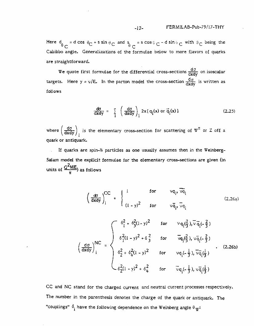
da We quote first formulae for the differential cross-sections - dxdy on isoscalar
da targets. Here y = u/E. In the parton model the cross-section - dxdy is written as
follows
& = C ( &) 2X[qitX) or<i(x)l 1 i
(2.25)
is the elementary cross-section for scattering of W’ or 2 off a
If quarks are spin-!4 particles as one usually assumes then in the Weinberg-
Salam mode1 the explicit formulae for the elementary cross-sections are given (in
units of G*l as follows
Q cc 1 for
( 1
‘qi9 Gi
dxdyi = (1 - y12 for ‘Tii, ‘4i
(2.26.4
c 6; + $(l- yJ2 for ’ qit~ ),‘sit- $1
i
for
6: + $1 - yj2 . (2.26b)
for ‘qit- ~ ), ~~i(~ )
$1 - yJ2 + 6; for
CC and NC stand for the charged current and neutral current Processes resPectivelY-
The number in the parenthesis denotes the charge of the quark or antiquark. The
“couplings” 6. have the following dependence on the Weinberg angle 8 w: 1
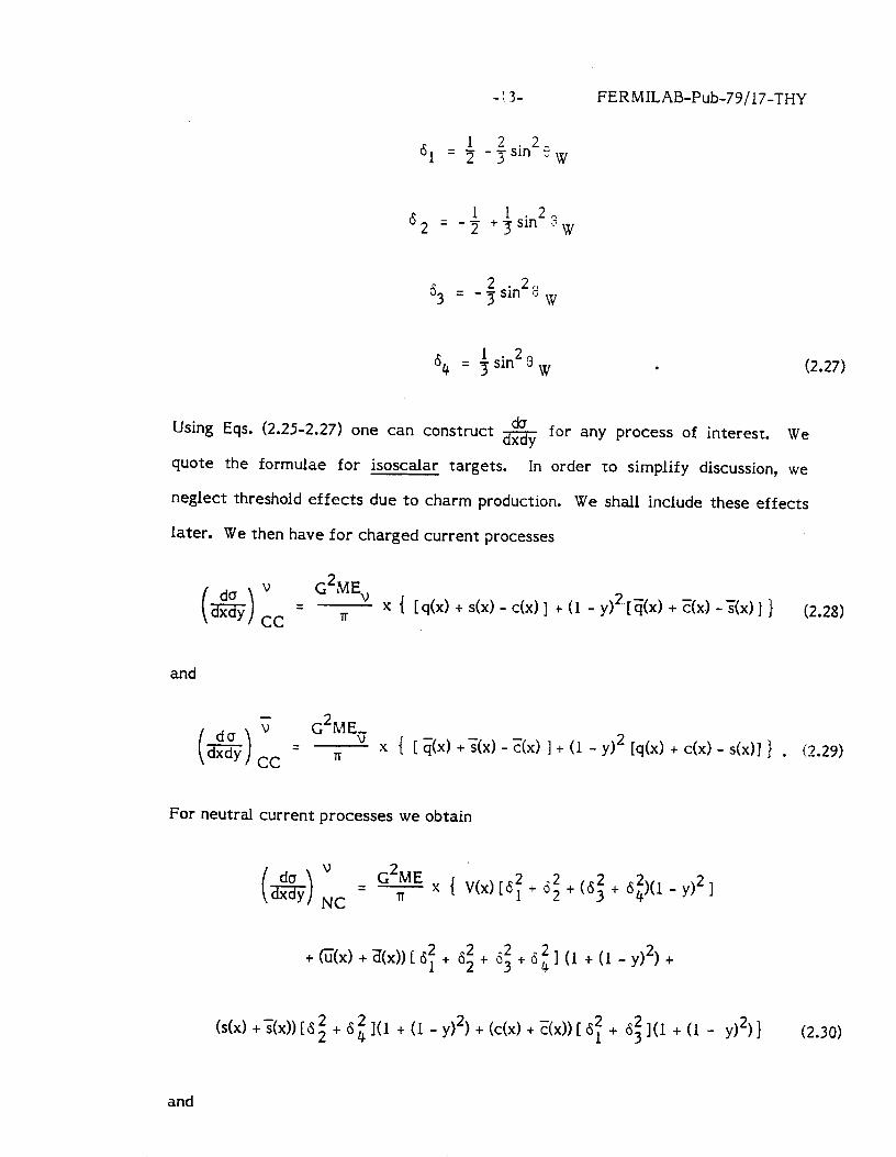
- : 3- FERMILAB-Pub-79/17-THY
1 cS1 = 7 - $sin2e w
62 = _ -jj- + f sin2 3 w
~5~ = - $ sin23 w
64 = $ sin2 8 w . (2.27)
Using Eqs. (2.25-2.27) one can construct do - for any process of interest. We dxdy quote the formulae for isoscalar targets. In order to simplify discussion, we
neglect threshold effects due to charm production. We shall include these effects
later. We then have for charged current processes
G’ME,
7T x t [q(x) + s(x) - c(x) ] t (1 - y)‘-[$x1 + 3X”) - S(x) II and
x { [ ;T<x> + ax> - ax> 1 + (1 - yJ2 [q(x) + c(x) - s(x)]
For neutral current processes we obtain
= G2ME Tr
+ (c(x) + 3(x)) c cs; + 6; + 6; + tit 1 (1 + (1 - yJ2) +
Md +3xM6; + 6; I(1 + (1 -yJ2) + (c(x) +Z(x))[$ + @l + (1 - y)2)}
(2.28)
. (2.29)
(2.30)
and
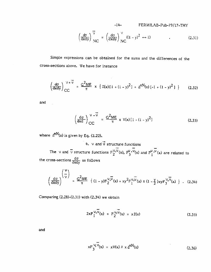
-14- FERMILAB-Pub-79/17-THY
(&) “,, = (&) ;,((I - YJ2 - 1) . (2.31)
Simple expressions can be obtained for the sums and the differences of the
cross-sections above. We have for instance
da dxdy { W[l + (1 - Y121 + AeN r-1 + (1 - yJ2 ] 1 (2.32)
and
( 1
v -7
ais- cc
2 = G+ x V(x)[l - (1 -y)21 (2.33)
where AeN is given by Eq. (2.22).
4. v and 3 structure functions
The V and 5 structure functions F~]?‘(x), F;“(x) and Fy 9’ (x) are related to do the cross-sections - dxdy as follows
= + { (1 - y)F;“(x) + xy2F;“(x) k (1 - f )xyF&) ) . (2.34)
Comparing (2.28)-(2.31) with (2.34) we obtain
2xF$x) = F;&x) = x C(x)
and
xF;‘(x) = XV(X) T x AeN
(2.35)
(2.36)
-1% FERMILAB-Pub-79/17-THY
for charged currents, and
and
2xF;‘v(x) = F;+(x) = Xc(X)[ 6; +6; + 6; + a;]
xF&) = XV(X) [ 6; + 6; - 6; -6; 1
(2.37)
(2.38)
for neutral currents.
Notice that FyVv (x) for both neutral current and charged current processes
behaves as non-singlet whereas F;’ for charged current processes behaves as a
pure singlet. Fipv for neutral current processes contains similarly to electromag-
netic structure functions (Eqs. 2.20 and 2.21) both singlet and non-singlet
contributions.
5. Basic properties of the simple parton model
There are many consequences of parton model ideas which have been
extensively discussed in the literature (e.g. Feynman, 1972; Llewellyn-Smith, 1972;
Landshoff and Polkinghorne, 1972; Close, 1979). We only mention few of them. F6 First there is Bjorken scaling in x for the structure functions and in x and y for the
da dxdy
cross-sections. This means for instance that < y > and c; /u,~ are energy
independent and the moments of the structure functions
dx Xn-2Fi(X) 5 M i(n) n = 2,3,...
0 i = 1,2,3,L (2.39)
are Q2 independent.
-16- FERMILAB-Pub-79/17-THY
Furthermore there exist certain sum rules and relations between structure
functions which deserve attention. These are in particular:
i) Adler Sum Rule (Adler, 1966)
1,l+ [e-F;p] = 2
ii) Gross-Llewellyn-Smith sum rule (Gross and Llewellyn-Smith, 1969)
J.oldx[@+F;p] = +6
iii) Bjorken Sum rule (Bjorken, 1967)
1
Jd[ x Fl %F;p = 1
0 1 and
iv) Callan-Gross reiation (Callan and Gross, 1969 )
F2 = 2xFl
(2.40)
(2.41)
(2.42)
(2.43)
or consequently FL = 0.
We should also remark that the parton model has been extended to other than
deep-inelastic processes. Famous examples are
e+e- + m+ anything
e+e- + hadrons
pp + u ‘u - + anything (2.44)
-17- FERMILAB-Pub-79/17-THY
and large pl processes.
The building blocks of all parton model formulae for processes listed under
(2.44) are again quark distributions (and fragmentation functions) which also enter
the deep-inelastic formulae. Consequently in the parton model there exist many
relations between various different processes. This fact as well as the simplicity
and intuitive picture behind the parton model already attracted many physicists ten
years ago. In spite of the successes of the parton model in the past, this model now
seems to be too simple to explain the data. In fact although Bjorken scaling is well
satisfied for 0.15 LX 2 0.25 over the relevant (deep-inelastic) Q2 range explored by
present experiments (2 2 Q22 100 GeV2), for x c 0.15 and x >0.25 definite Q2
dependence is seen in the data for ep and u p scattering. Similar scaling violations
have been observed in high energy v ,J processes. In addition, the ratio R = o L/o T
as measured in ep scattering is definitely different from zero contrary to equation
(2.43). AU th ese facts indicate that we have to go beyond the simple parton model
if we want to understand the data.
6. Beyond the simple parton model
Even before the discovery of scaling violations in deep-inelastic scattering
theorists found a beautiful interacting (Gauge-) Field Theory-Quantum Chromody-
namics with its property of asymptotic freedom and calculable pattern of scaling
violations. As we shall see in the course of this review, this theory has not only
much better theoretical background than the simple parton model but also fits
better the existing data. In addition in spite of a very heavy mathematical
machinery the predictions of the theory in question have a very simple intuitive
interpretation similar to the simple parton model but much richer.
It is perhaps useful to get a general overview and list how the simple parton
model properties are modified in asymptotically free gauge theories (ASF).
-18- FERMILAB-Pub-79/17-THY
First we write symbolically the ASF predictions for the moments of the
structure functions as follows
Ii dx x n-2F(x, Q2) = A,., [ln Q2 1 -dn 0
l+ fn - + . . . In Q2
(2.45)
where An, dn and f, are numbers to be discussed in the subsequent sections. Then
in the leading order (first term on the r.h.s. of equation Q..45jj, all parton model
formulae of this section remain unchanged except that now the parton distributions
depend on both x and Q2. in particular, all sum rules (e.g. 2.40-2.43) are satisfied.
The Q2 dependence of parton distributions is calculable.
During this past year it became clear that also parton model relations
between various processes (deep-inelastic scattering, Drell-Yan process, etc.) also
remain unchanged in the leading order.
On the other hand, if next-to-the-leading terms are taken into account (e.g.
second term in Eq. 2.45), sum rules (e.g. -. 7 41-2.43) are violated. One also expects
beyond the leading order corrections to the parton model relations connecting
‘various processes.
C. Basic Formulae of Asymptotic Freedom
In this Section we shall collect all asymptotic freedom formulae relevant for
phenomenological study of deep-inelastic scattering. The derivations, discussions
and intuitive interpretations of the formulae below, can be found in Sections III to
VIII.
1. Leading order
In the leading order of asymptotic freedom all parton model formulae of
Section 1I.B remain unchanged except that now parton distributions depend on Q2.
In Quantum Chromodynamics the Q2 dependence of parton distributions is given by
certain equations, which we present now.
-lY- FERMILAB-Pub-79/17-THY
1.1. Effective coupling constant
Contrary to the simple parton model, which corresponds to a free Field
Theory, QCD is an interacting field theory. The interactions between quarks and
gluons can be described by the effective coupling constant i2(Q2) which satisfies
the following equation
where
t=lnQ1 l.12
(2.46)
(2.47)
and g is the renormalized coupling constant. Furthermore B(g) is a renormalization
group function and p2 is the subtraction scale at which the theory is renormalized.
The presence of this scale is at the origin of scaling violations. The notion of B(g)
and of p2 will be given in Section III. Here it suffices to say that l3(g) can be
calculated in perturbation theory. We have
B(g) = - B, 32 - B, _8, + . . . 16n2 (161~~)
(2.48)
The parameters 8, and Bl have been calculated by (Politzer, 1973; Gross and
Wilczek, 1973a)and (Caswell, 1974; Jones, 1974) respectively. In QCD (SU(3) gauge
theory) they are given as follows
8, = 11 -$f (2.49a)
-2o- FERMILAB-Pub-79/17-THY
and
B, = 102 -T f . (2.49b)
Here f is the number of flavors.
Keeping only the first term on the r.h.s. of equation (2.48) and inserting B(g)
into Eqs. (2.46) one obtains the leading order formula for i2(Q2):
g2(Q2) = 16~~ 2
so+
The scale parameter A is related to 1-1 and g as follows
A2 = p2 exp 16r2 [ 1 Bog2
(2.50)
(2.51)
A is a free parameter which is to be found by comparing QCD predictions with
experimental data. It follows from Eq. (2.50) that the effective coupling constant
decreases with increasing Q2 and vanishes for Q2 = *. This is what we mean by
asymptotic freedom.
1.2 Intuitive approach
In the intuitive approach to asymptotic freedom (Kogut and Susskind, 1974f!o
be discussed in detail in Section V one imagines that by increasing Q2 of the photon
or W boson or equivalently by probing the inner structure of the hadron at smaller
distances one can resolve the quark into a quark and a gluon, gluon into quark-
antiquark pair and gluon into two gluons. These three basic processes are shown in
Fig. 3. It follows immediately from this picture that the parton distributions
depend on Q2. On a more quantitative level (Parisi, 1975; Altarelli and Parisi,
-21- FERMILAB-Pub-79 /I ‘/-THY
1977; Dokshitser, Dyakonov and Troyan, 1978a) one introduces “splitting” functions
Pij(z) which are the measure of the variation (with Q2) of the probability of finding a
parton i inside the parton j with the fraction of the parent momentum z = x./x.. Then ’ 1
the equations which determine the Q2 dependence of the parton distributions are given
as follows
dAi’(X, t) dt
ddx, t) = dt % s ‘* b(,, t)Pqq$ ) + 2f G(y, t)PqG(f )]
x y
dG(x, t) = ‘-O dt t* +, t)PGq(; ) + G(y, f)PCG(; )] 2lr xY C
(2.52)
(2.53)
(2.54)
where C , A ij and t have been defined in Eqs. (2.16), (2.17) and (2.47) respectively.
Furthermore
(2.55)
and ~j(X, t) defined in Eq. (2.18) satisfies Eq. (2.52).
The functions Pij(z) are explicitly given in QCD (Altarelli and Parisi, 1977;
Dokhsitser, Dyakonov and Troyan, 1978). They are
Pqq(z) = ; (& +; L
&(I - z) + 1
pqG(z) = ; [ z2 + (1 - z)2 1 (2.56)
(2.57)
-22- FERMILAB-Pub-79/17-THY
4 1 + (1 pGq(z) = 7 z - z)2 (2.58)
and
‘GGb) = 6 c (+ + 7 (1 - z, + z(l - z) + (; -A) a(1 -z)j . (2.59)
The distribution (1 - z);’ is defined by the following equation
I ' dz & 2 0 +
J' ' dz f'z/l-wf$' 0
(2.60)
where f(z) is any function regular at the end points. For z < 1, (1 - z)+ = 1 - z. The
properties of the splitting function Pii and of the solutions of Eqs. (2.52)-(2.54)
are discussed in Section V.
Finally we want to comment on how the integro-differential equations above
can be used in the phenomenological applications. One assumes or takes from the
data the distributions Aij(x, Qz), ,X(x, Qz) and G(x, Qi) at a certain value of
Q2 = Qz. These distributions serve as the boundary conditions for Eqs. (2.52)-(2.54)
which can be solved numerically. For practical purposes before writing a computer
program it is useful to get rid of terms (1 - z)L1 by employing the following formula
II H@ = H(x)ln(l - x) + I ’ dz
X dz Zl-izJ+ x (l-i) ( zH$) - H(x)) (2.61)
where H(x) is any function regular at the end points.
-23- FERMILAB-Pub-79/17-THY
1.3 Formal approach
In the formal approach to asymptotic freedom (Gross and Wilczek, 1974;
Georgi and Politzer, 1974) to be discussed in detail in Section IV one uses the
operator product expansion (Wilson, 1969) for the product of currents which enter
Eq. (2.1). We write symbolically
X2)30) = 1 ?(z2)z 0 +- 4-l i,n pl”‘Zpn i (2.62)
F8 where the sum runs over spin n, twist 2 operators such as the fermion non-singlet lJ”I”’ b
operator ONS and the singlet fermion and gluon operators 0 1-I 1”‘un and
+**I+) 9
OG ’ respectively. Explicit expressions for these operators are given in
Section III. w i Cn(z2) are the Wilson coefficient functions. We next define the
reduced matrix elements, A’ n, of the operators in question as follows
lJ1...un <PlO. I Ip > = A;p, . ..pu
1 n
Then we can write (Christ, Hasslacher, Mueller, 1972)
II dx x”-~F~(x, Q2) = 1 0 i
A$r2)C’k n I
(2.63)
(2.64)
(x, Q2) is an arbitrary deep-inelastic structure function (k = 1,2,3,L) and
are fourier transforms of the coefficient functions in Eq. (2.62).
Notice that in writing (2.64) we have been more explicit than in Eq. (2.62),
indicating that the coefficient functions depend on the structure functions
involved, and that the coefficient functions can be calculated in perturbation
theory in g. We have also indicated that the reduced matrix elements Ain depend
on P2.
-‘ii& FERMILAB-Pub-79/17-THY
As discussed in Section III there is a set of non-singlet operators corres-
ponding to various XK in Eq. (3.55). Since these operators neither mix under
renormalization with each other nor with the singlet operators, the Q2 dependence
of their coefficient functions is in common. Therefore in this review any linear
combination of non-singlet operators will be denoted for simplicity by a common 1-I l...pN
symbol ONs and the corresponding reduced matrix elements and coefficient
functions by An NS(u2) and C’;Irn(Q2/u2, g2) respectively. It should however be kept
in mind that AyS (u 2 ) depend generally on the process and the structure function
considered. This dependence is discussed in Appendix 8.
The Q2 dependence of the Wilson coefficient functions is governed by certain
equations called renormalization group equations which for the coefficient
functions of non-singlet operators take the following simple form
(2.65)
Here uis(g) is the anomalous dimension of the spin n non-singlet operator and B(g)
has been defined in Eq. (2.46). The renormalization group equations are discussed
in Sections III and IV. Here it suffices to give the solution of Eq. (2.65) which is
(2.66)
The 1 on the r.h.s. of Eq. (2.66) means simply Q2 = v2.
CF,:(l, g2) and y;,(g) can be calculated in perturbation theory. Up to and in-
cluding next-to-leading order corrections we have
k ’ NS
1 + i? BNS 161~~ k9n
k = 1,2,3
(2.67) I dL NS O+xBNS
16a2 L’n
-2% FERMILAB-Pub-79/
and
y Fls (l),n +yNS
g4
t16r2j2 ’
.7-THY
(2.68)
where Btyn, ysvn and ytifn are known numbers to be specified below. 6 & are
constants which depend on weak and electromagnetic charges. Specific examples
of c$& are given in Appendix B. Perturbative expansion for /3(g) is given in Eq.
(2.48).
In the leading order one keeps only the first terms on the r.h.s. of Eqs. (2.48),
(2.67) and (2.68). Then using (2.64), (2.66) and (2.50) one obtains a general
expression for the Q2 evolution of the moments of any non-singlet structure
function Fy
+S k = 1,2,3
0 dx x”-‘F;‘(x, Q2) =
where
O&n d” ‘NS --
NS- 2B 0
k=L (2.69a)
(2.70)
and we have put u 2 = Qz. (Oh The parameters yNs have been calculated by (Georgi
and Politzer, 1974; Gross and WiIczek, 1974) and are given as follows
$in = 8 3 l- c (2.71)
-26- FERMILAB-Pub-79/17-THY
Except for the value of A, the only unknown parameters in Eq. (2.69a) are the
Ai’( They can be determined from experiment by measuring Fk NS(x, Qt) at an
arbitrary value of Q2 = Q,. 2 Flf. mce the value of Qz in Eq. (2.69a) is arbitrary, as
required by the renormalization group equations, it is often convenient to get rid of
Qz by writing Eq. (2.69a) as follows
dx x”-~F~~(~, Q2) = 6ks /fS -d”NS
k = 1,2,3 0
(2.69bI
Here ANS n are (independent of Qi) constants which are related to An “‘(Qi) by Eq.
(4.19).
For singlet structure functions the situation is more complicated because, as
discussed in Section III, the operators Or$i, and 02 mix under renormalization. The
Q2 dependence of the corresponding Wilson coefficient functions Cl n and Ct n is 9 9 governed by two coupled renormalization group equations
[ P & + B(g)&
I ( c’k n
2 Q 9 112
Here $(g2) are the elements of
following perturbative expansion
9g 2 i,j = $,G . (2.72)
the anomalous dimension matrix. They have the
Y;(gZ) (Oh J& = Yji + y(l,,n g4 16n2 I1 (16~~)
2 + . . . . (2.73)
We shall discuss the solution of Eq. (2.72) in Section IV. Here it is sufficient to give
the generalization of Eqs. (2.69a,b) to any singlet structure function F$x, Q2). In
the leading order we have
j- l dx x”-~F;(x, Q2) = 0
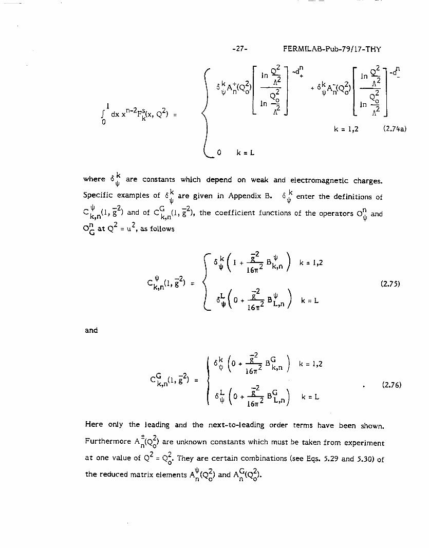
-27-
ln$
Q2 In 0
Ii2
FERMILAB-Pub-79/17-THY
k = 1,2 (2.74a)
c 0 k=L
where 6 k $
are constants which depend on weak and electromagnetic charges.
Specific examples of 6; are given in Appendix B. Lsk JI enter the definitions of
CQ, i2) and of Ct .(l, g2), the coefficient functions of the operators 0; and 9
0°C at Q2 = p2, as follows
k = I,2
and
I k = 1,2
C$l, i2, =
k=L
(2.75)
. (2.76)
Here only the leading and the next-to-leading order terms have been shown.
Furthermore Af(Qz) are unknown constants which must be taken from experiment
at one value of Q2 = Qz. They are certain combinations (see Eqs. 5.29 and 5.30) of
the reduced matrix elements A$Qz) and Ai(Q$
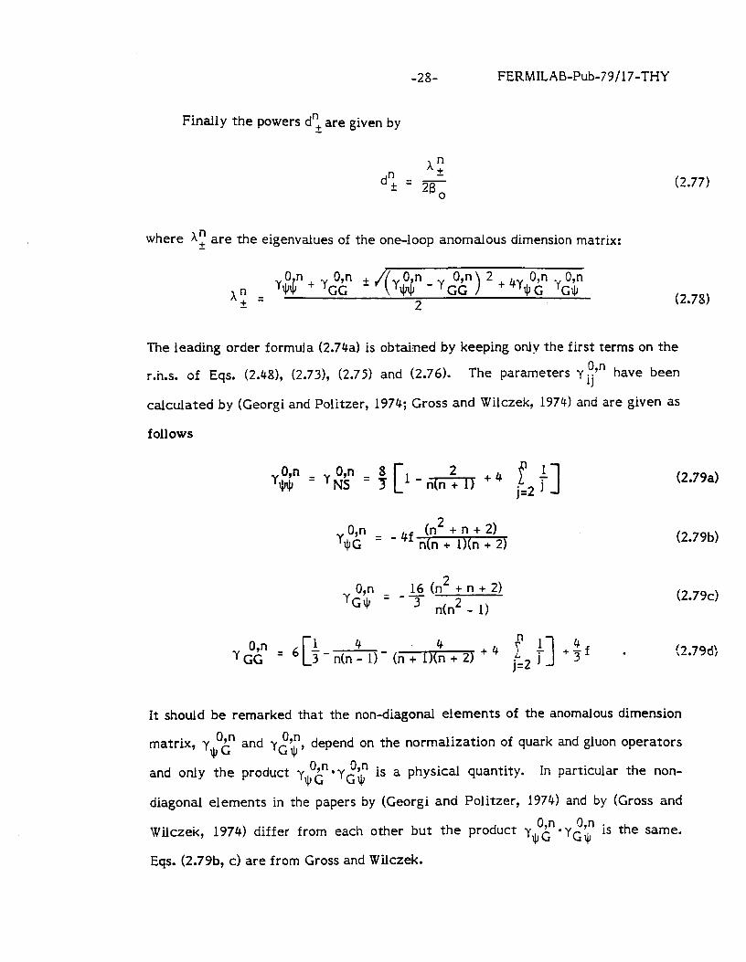
-2% FERMILAB-Pub-79/17-THY
Finally the powers dr’+ are given by
A” ?c d; = 28
0 (2.77)
where “2 are the eigenvalues of the one-loop anomalous dimension matrix:
Y$)$” + Y$J f /( f&n A”
Y$” - Y GG >
2 + 4y$Okn pin
+ = 2 (2.78)
The leading order formula (2.74a) is obtained by keeping only the first terms on the
r.h.s. of Eqs. (2.48, (2.73), (2.75) and (2.76). The Parameters
calculated by (Georgi and Politzer, 1974; Gross and Wilczek, 1974)
follows
y 04 ij have been
and are given as
y$=y$L; l- 1
2 1 Iii +4
j=2 T f 1 y;g = - 4f (n2 + n + 2)
n(n + l)(n + 2)
16 (n2 + n + 2) Yco3 q - 3 n(n2 _ 1)
y&? = 6 1 4 4 7-n(n-l)‘(n+l)(n+2) +4 +- if .
(2.79a)
(2.79b)
(2.79~)
(2.79d)
It should be remarked that the non-diagonal elements of the anomalous dimension
matrix, yJpo($ and yGo;“, depend on the normalization of quark and gluon operators
and only the product y $0;” .y;$ is a physical quantity. In particular the non-
diagonal elements in the papers by (Georgi and Politzer, 1974) and by (Gross and
Wilczek, 1974) differ from each other but the product yQokn l y,-$ is the same.
Eqs. (2.79b, c) are from Gross and Wilczek.
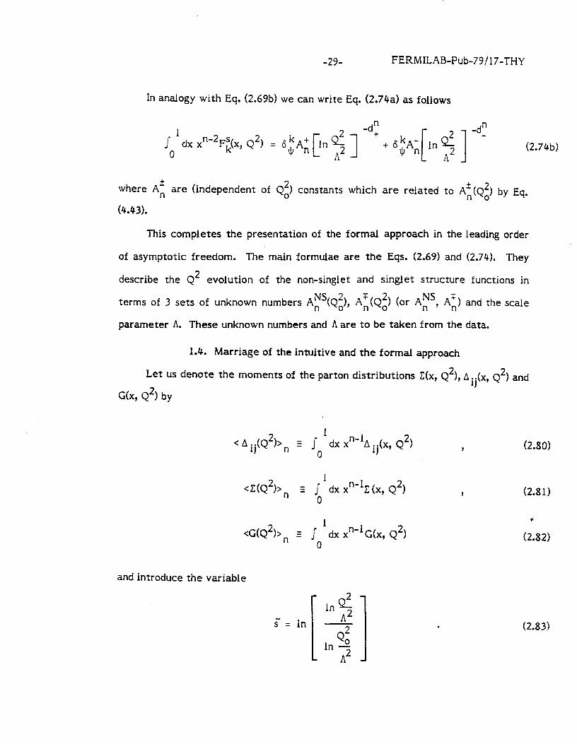
-29- FERMILAB-Pub-79/17-THY
In analogy with Eq. (2.69b) we can write Eq. (2.74a) as follows
‘,Idx x”-~F$x, Q~) = $A; [In d ] -d;
A2 (2.74b)
where Ai are (independent of Qz) constants which are related to Ai by Eq.
(4.43).
This completes the presentation of the formal approach in the leading order
of asymptotic freedom. The main formulae are the Eqs. (2.69) and (2.741. They
describe the Q2 evolution of the non-singlet and singlet structure functions in
terms of 3 sets of unknown numbers An “(Q$, AE(Qz) (or AtS, AX) and the scale
parameter A. These unknown numbers and A are to be taken from the data.
1.4. Marriage of the intuitive and the formal approach
Let us denote the moments of the parton distributions C(x, Q2), Aij(x, Q~) and
G(x, Q2) by
< A ij(Q’)>, 3 s 1
0 dX X"-lA ij(X, Q2) 9
cC(Q'),, z s 1
dx ~“-11 (x, Q2) 3 0
<c(Q2bn z s 1
dx x”-lG(x, Q2) n
and introduce the variable
s” = In
J
ln$
Q2 In o
A2
(2.80)
(2.81)
c
(2.82)
(2.83)
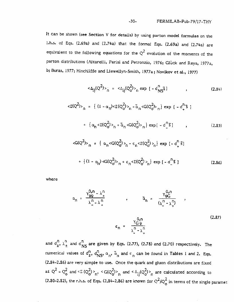
-3o- FERMILAB-Pub-79/17-THY
It can be shown (see Section V for details) by using parton model formulae on the
1.h.s. of Eqs. (2.69a) and (2.74a) that the formal Eqs. (2.69a) and (2.74a) are
equivalent to the following equations for the Q2 evolution of the moments of the
parton distributions (Altareili, Parisi and Petronzio, 1976; Gliick and Reya, 1977a,
b; Buras, 1977; Hinchliffe and Llewellyn-Smith, 1977a; Novikov et al., 1977)
<Aij(Q’)>n = <Aij(Q~)>n exp [ - dLsZ ] 9
<c(Q’)>, = ( (1 -ankC(Qz)>n -TU,CG(Q~)>~} exp E - d”3 1 +
+ { an <c(Qf$ >n + En <G(Qzb n ) exp i - d”:] 9
4Q2bn = { anG(Q;) ‘n - E,,<E(Q~) >n} exp [- ciy :I
+ { (1 - c+J <G(Qzbn + E,<C(Q~) >n} exp [ - d”g 1
(2.84)
i2.85)
(2.86)
where
an = yg - xy
A”- A:
(2.87)
and d:, n A, and diS are given by Eqs. (2.77), (2.78) and (2.70) respectively. The
numerical values of d”,, d” NS, an, sn and E n can be found in Tables 1 and 2. Eqs.
(2.84-2.86) are very simple to use. Once the quark and giuon distributions are fixed
at Q2 = Qz and <C (Qz) >n, <G(Qt)>, and <Aij(Qz)>n are caIculated according to
(2.80-2.82), th e r.h.s. of Eqs. (2.84-2.86) are known for Q 2 2 #Q, in terms of the single paramet
-31- FERMILAB-Pub-79/17-THY
A. This parameter can be found by fitting the left-hand side of the equations in
question to the data (see however discussion in Section VII). We shall demonstrate
in Section V that equations (2.84)-(2.86) are equivalent to the integro-differential
Eqs. (2.52)-(2.54).
This completes the presentation of the asymptotic freedom formulae in the
leading order.
2. Higher order corrections
In the literature most of the discussions of higher order asymptotic freedom
corrections have been done in the formal approach of Section 1.3. We shall begin
with this approach. Higher order asymptotic freedom formulae, expressed in terms
of parton distributions, will be given at the end of this Section.
2.1 Effective coupling constant
The solution of Eq. (2.46) with B(g) given by
inverse powers of In 2 A2
with the result
*2
z2(Q2) 16n2
= 1 -
B,ln d A2
% 7
0
In In C A2
in2 C?Z A2
Eq. expanded in
. (2.88)
Here and following (Buras, Floratos, Ross and Sachrajda, lY77)Fihas been chosen so
that there are no further
p2, A2 and g2 are related
terms of order l/(ln2 Q2/A2). A little algebra shows that
to each other by
7 AL = p 2 exp 167~~ 81 - - - - ln( !30g2)
1 . (2.89)
Eqs. (2.88) and (2.89) are generalizations of Eqs. (2.50) and (2.51), respectively.
-32- FERMILAB-Pub-79/17-THY
In what follows we want to present the corresponding generalizations of Eqs. (2.69)
and (2,74). The derivation of the formulae below is presented in great detail in
Sections VII and VIII.
2.2. Non-singlet structure functions
For non-singlet structure functions which do not vanish in the leading order,
namely FyS, FFS and FyS, the generalization of Eqs. (2.69a) and (2.69b) are given
as follows
MN% Q2) - 6 k k ’ - NsAfstQ;)
[ lnQ1.
A2 Q2 In o
A2
1 -dkS
k = 1,2,3 (2.90a)
J
and
Mrs (n, Q2) = 6 #:" c 1
ln$ -dFJS
A2 k = 1,2,3 (2.90b)
where Afs are (independent of Qz) constants which are related to At’(Q$ by
Eq. (7.22). Furthermore
where
(l),n RNS ‘NS
(Oh
k,n = Br,t ’ 28 - - ‘NS f3
k = 1,2,3 0 28; l ’
(2.91)
(2.92)
The parameters Bfz and ygin ? have been defined in Eqs. (2.67) and (2.68)
respectively and d” NS is given by Eq. (2.70). For the longitudinal structure function
we have
-33- FERMILAB-Pub-79/17-THY
SO1 & x”-~F~~(x, Q2) = L
&NS
NS BL,n
lnQf A2 [ I 2
In Q. 7
-d”Ns (2.93)
where Bysn is defined in Eq. (2.67). Because the longitudinal structure function 9
vanishes in the leading order it follows that in the order considered An NS(Qi) is the
same as in Eq. (2.69a). Furthermore in obtaining (2.93) the leading order formula
for g2(Q2) (2 50) should be used. It turns out that 6 (2) - gL ? l 9
NS - NS
and therefore Eq.
(2.93) can be written as follows (Zee, Wilczek, Treiman, 1974)
s1 0
dx x~-‘F;~(,, Q2) = BNS
L+-’ s l dx x”-~F;?x, Q2) 1
B lnQ1 O
(2.94)
A2 LO
0
where “LO” indicates that the moments of F2 NS(x, Q2) are given by the leading
order expression (2.69).
Finally we give formulae for Brt (l),n 9
and numerical resuits for yNs . The
parameters NS BL n have been calculated by (Zee, Wilczek and Treiman, 1974) and are ?
given as follows
BNS 16 1 bn = mm . (2.95)
BNS NS 1 ,n’ B2,n and By: have been calculated by (Bardeen, Buras, Duke, Muta, 1978) 9
and recalculated by (Floratos, Ross, Sachrajda, 1979f 12,F13 They are given as follows
BNS 3 { ? 1 n 2,n =
'jl,l~' 4I~-&J n 1
1 1
j=l 1 j=l ‘j-
(In h - yEI , (2.96)
-34-
BNS Ln
= By; - By; ? ,
and
BNS NS 4 4n+2 34 = B2,n -3 iii)
FERMILAB-Pub-79/ 17-THY
(2.97)
. (2.98)
The constant yE is the Euler-Masheroni constant yE = 0.5772... We shall comment
on the terms (In 4~ - yE) in subsection 2.5.
I l),n The two-loop anomalous dimensions -{is have been calculateo by (‘t%ratos,
Ross and Sachrajda, 1977). We give only their numerical values in Table 3 since the
corresponding analytic expressions in the original paper are rather complicated.
(l),n Relatively simple analytic expressions for yNs can be found in the paper by
(Gonzalez-Arroyo, Lopez and Yndurain, 1978).
2.3. Corrections to parton model sum rules
It follows from Eqs. (2.95) to (2.98) that the sum rules (2.41) to (2.43) are no
longer satisfied. The Adler sum rule (2.40), which expresses charge conservation,
is, however, still respected. We have (Bardeen, Buras, Duke, Muta, 1978; Altatelli,
Ellis, Martinelli, 1978)F’4
F;p+F;p] = 6 l- [ (33-Zln$]
and
‘,’ dx [F\Ip - Fyp] q ’ 1 -(33 28) 1 2
n A2 The violation of Callan-Gross relation (2.43) is expressed by Eq- (2.94).
(2.99)
(2.100)
-35- FERMILAB-Pub-79/17-THY
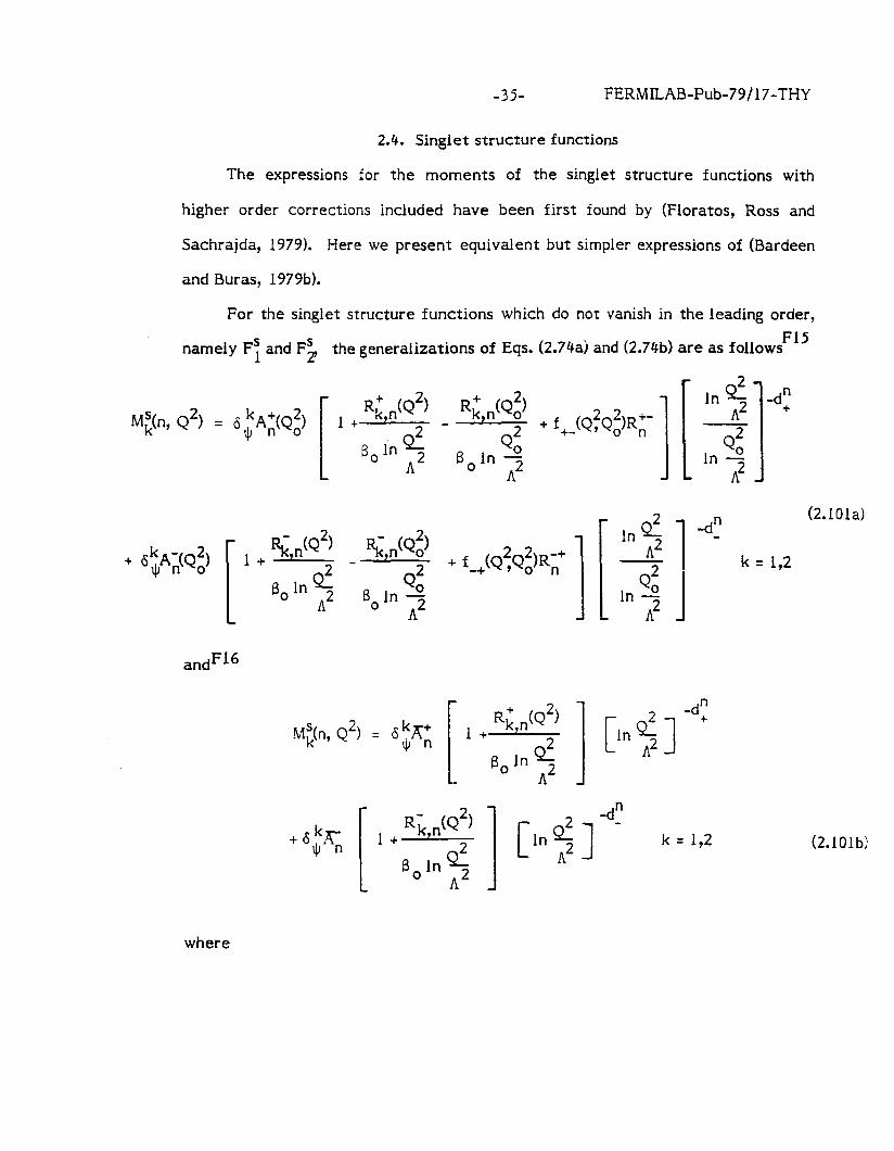
2.4. Singlet structure functions
The expressions for the moments of the singlet structure functions with
higher order corrections included have been first found by (Fioratos, Ross and
Sachrajda, 1979). Here we present equivalent but simpler expressions of (Bardeen
and Buras, 1979b).
For the singlet structure functions which do not vanish in the leading order,
namely Fs and F!,, the generalizations of Eqs. (2.74aj and (2.74b) are as follows F15
M$n, Q2) = &$Ai(Q$ R+ (Q2)
1 + k,n 2 3,ln Q
A2
Rk’ ,(Qz)
Q2 + f ._(QfQ;)R;-
B,ln o A2
+ +-,(Q;) R,&Q2)
-2
Bo In 3 1L
$ ,(Q ;)
Q2 B, In o
A2
+ f -+tQ;Q;)R;+
I [
ln$
Q2 In 0
A2
1 1 J
In 5
I
-d” +
Q2 In 0
A2
-d_”
k = 1,2
andF16
M$n, Q2) = 6t??n 1 + Rc n(Q2) ’ I 2 r 1 ln$
-d’:
B, In e A2
A2
+ 6 kAW $ n
R- (Q2) 1 -t k,n -3
1 BolnQf A2
-d_” k = 1,2
(2.101a)
(2.101b)
where
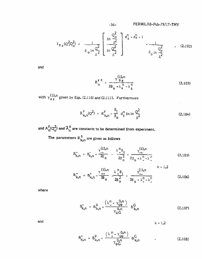
-36- FERMILAB-Pub-79/17-THY
dt - d: - 1
fTk(Q!Q;) = -- 1 Q2 7 (2.102)
3. In 0 A2
and
RT,* = y (lh
7+ 2B
0
with yp!ln given by Eqs. (2.110) and (2.11 I). Furthermore
2 R;,n(Q ) B
’ = R;,n - Fo F d” lnln 2 A2
and Ai and x,’ are constants to be determined from experiment.
The parameters Ri n are given as follows 9
where
and
+l),n pB %,n = S,n + 28 - $+ - 2~
,W,n 0
-+n +A -A
n ‘0 0 - f
R; n = B;,, y W,n x nB
+ 1 ++t---
y(l)4 k = I,2
+- 9 7 2fi; 2Bo+ x:-x”
k = 1,2
J, ( x n 0
Bk’,n = Bk,n ’ + - TJJQ >
BG k,n *
(2.103)
(2.104)
(2.105)
(2.106)
(2.107)
(2.108)
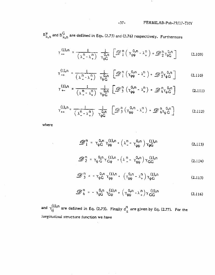
-37- FERMILAB-Pub-79/17-THY
B* G k n and B k n are defined in Eqs. (2.75) and (2.76) respectively. Furthermore 9 ,
y (lb = -- (2.109)
y(l),n = 1 1 -+
( A”- A;) YJpO&! - 9; Y$-x”)+ &Y$yJ r (
y(l)7n = 1 1 +-
( A”- $> Yq”g c ( 9; Y$- A:) + 9 qny$Ohn 3
yW,n = -I-+ (X”--x=>
where
(2.110)
(2.111)
(2.112)
(2.113)
(l),n yGG (2.114)
2%; = 04 (l),n - y$G YJ~,J, + (l),n
‘: ) y+G (2.115)
(2.116)
and $,l’ . . & are defined in Eq. (2.73). Finally d”, are given by Eq. (2.77). For the
longitudinal structure function we have
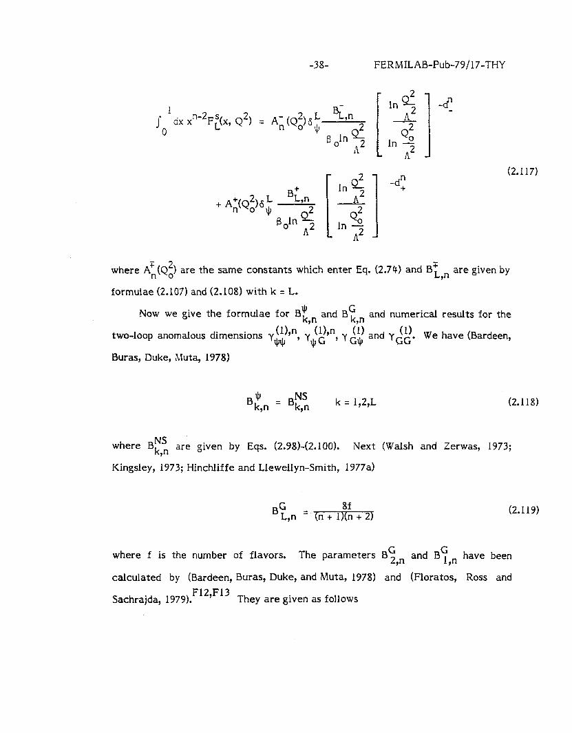
-38- FERMILAB-Pub-79/17-THY
dx x”-~F;(x,
Q2) 2 = A; (Q,)
6 L B;,n 0 +
3 oln Q2 2
12
+ A+(Q2)S L Bl,n n O 9
inPI A2 Q2
In 0 A2
In QZ -dh A2 - l- Q2
In o s A2
-d: (2.117)
where A’,(Qz) are the same constants which enter Eq. (2.74) and Bt n are given by 9 formulae (2.107) and (2.108) with k = L.
Now we give the formulae for Bt n G and B k.n and numerical results for the .
two-loop anomalous dimensions y (l),n ’ (l),n (1) (1) ,i,9 9 y,,, G * ‘Y Gi, and YGG* We have (Bardeen,
Buras, Duke, Muta, 1978)
B;,, = B;; k = 1,2,L 9 9 (2.118)
where BFz are given by Eqs. (2.98)-(2.100). Next (Walsh and Zerwas, 1973; 9
Kingsley, 1973; Hinchliffe and Llewellyn-Smith, 1977a)
BG 8f L,n = (n + I)(n + 2)
(2.119)
where f is the number of flavors. The parameters 8; n G and Bl,n have been 9
calculated by (Bardeen, Buras, Duke, and Muta, 1978) and (Floratos, Ross and
Sachrajda, 1979). F12,F13 They are given as follows
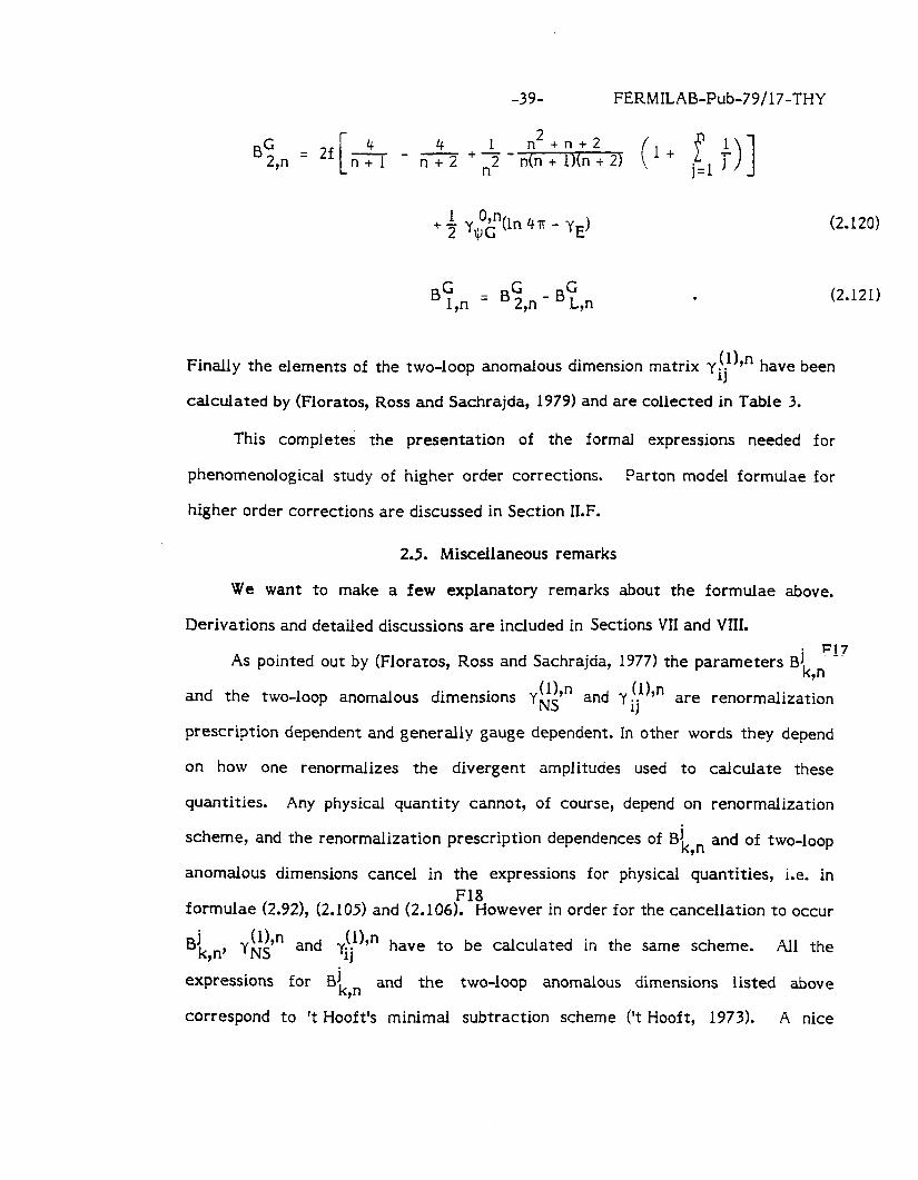
-39- FERMILAB-Pub-79/17-THY
BG 4 1 n*+n+2 n 1 2,n
= 2f [ 4 n+l
- n+2+-- n2 n(n + l)(n + 21
( 1+ j=l T c )I
BG G G 1,n = B 2,n - B L,n .
(2.120)
(2.121)
(114 Finally the elements of the two-loop anomalous dimension matrix Yij have been
caIcuIated by (Floratos, Ross and Sachrajda, 1979) and are collected in Table 3.
This completes the presentation of the formal expressions needed for
phenomenological study of higher order corrections. Parton model formulae for
higher order corrections are discussed in Section ILF.
2.5. Miscellaneous remarks
We want to make a few explanatory remarks about the formulae above.
Derivations and detailed discussions are included in Sections VII and VIII. . FIT’
As pointed out by (Floratos, Ross and Sachrajda, 19771 the parameters Blk n 9
(l),n and the two-loop anomalous dimensions yNs and yj;’ 4 . . are renormalization
prescription dependent and generally gauge dependent. In other words they depend
on how one renormalizes the divergent amplitudes used to calcuiate these
quantities. Any physical quantity cannot, of course, depend on renormalization
scheme, and the renormalization prescription dependences of Bjk n and of two-loop 9
anomalous dimensions cancel in the expressions for physical quantities, i.e. in Fl8
formulae (2.921, (2.105) and (2.106). However in order for the cancellation to occur
Bjk n, have to be calculated in the same scheme. All the 7 yEtn and y.(;)yn
expressions for Bk,n and the two-loop anomalous dimensions listed above
correspond to ‘t Hooft’s minimal subtraction scheme (‘t Hooft, 1973). A nice
-4o- FERMILAB-Pub-79 /17-THY
property of this scheme is that Bj W,n k,n’ yNS and y!ll) .. 4 calculated in this -scheme
are gauge independent (Caswell and Wilczek, 1974). Calculations of Bk n in other 9 schemes have been made by (Kingsley, 1973; Calvo, 1977; De Rujula, Georgi and
Politzer, 1977a; Altarelli, Ellis, Martinelli, 1978; Kubar-And& and Paige, 1979).Fly
The terms which involve (In HIT - y E) can be absorbed by redefining the scale
parameter A (Bardeen, Buras, Duke, Muta, 1978). Generally this can be done with
any term in Rlk n proportional to y i;” in the case of non-singlet structure 9
functions and with any term proportional to X, n in the case of singlet structure
functions. This freedom of defining A is related to the freedom of defining the
effective coupling constant when solving the renormalization group equations.
Therefore a numerical value of A extracted from experiment on the basis of
higher order formulae only has a meaning if the definition of the effective coupling
constant is given at the same time. The same comment applies to numerical values s F20
of parameters Rt( n. We shall give specific examples in Section VII. 9
D. Mass Corrections
SO far in this review we have discussed only the scaling violations due to QCD
effects. Certainly at low values of Q2 3 0 (few GeV2) target mass, heavy quark
mass effects and higher twist corrections will not be negligible. Here we shall indicate ho
the formulae presented above are modified in the presence of masses. We shall comment o
higher twist contributions later on.
In the last two years there has been a lot of progress in the understanding of
mass corrections in the framework of QCD but we think the question is not
completely solved. Neglecting the warnings for a moment which will be made
subsequently, the modifications due to mass effects in the formulae above are as
follows. We shall discuss here only target mass corrections and mass corrections in
the case of heavy quark production off light quarks in v and 7 scattering. More
general cases are discussed by (Georgi and Politzer, 1976) and (Barbieri, Ellis,
Galllard and Ross, 1976a, b).
-4l- FERMILAB-Pub-79 / 17-THY
1. Target mass-corrections
In Section 1I.C we have seen that asymptotic freedom predictions are
particularly simple when given for the moments (Cornwall and Norton, 1968)
1 Mh Q2) = j- dx x”-~F(x, Q2)
0 (2.122)
since to each given moment (n - 2) and for large values of Q2 only a small number
of operators of a given spin n (so-called twist-2 operators) contribute.
For lower values of Q2 the mass effects are non-negligible and this is no
longer true. In fact there are infinitely many operators of leading twist and
different spin which contribute to the n-th moment in the presence of masses. It
has been demonstrated by Nachtmann (1973) however, that one can redefine the
moments (2.122) in such a way that to the (n-2) moment only operators of spin n
will contribute as in the massless case.
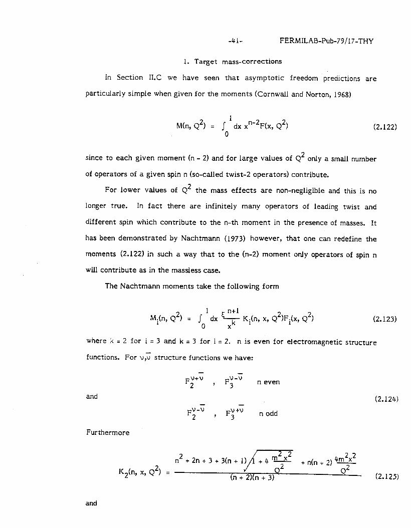
The Nachtmann moments take the following form
Mi(n, Q2) = l ‘dx * 0 Xk
Ki(n, x, Q’)Fi(x, Q2) (2.123)
where k = 2 for i q 3 and k = 3 for i = 2. n is even for electromagnetic structure
functions. For v,; structure functions we have:
p+v 2 , F;-’ n even
and
Fv-v 2 , F;” n odd
Furthermore
(2.124)
n2 + 2n + 3 + 3(n K2(n, x, Q2) =
+ l#T +n(n+2)
(n + 2)(n + 3) (2.125)
and
-42- FERMILAB-Pub-79/17-THY
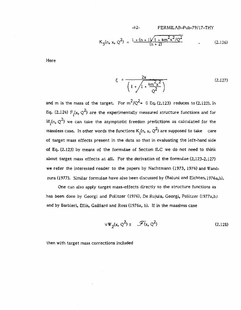
K3(n, x, Q2) =
Here
l+(n+l) (n + 2) . (2.126)
(2.127)
and m is the mass of the target. For m2!Q2+ 0 Eq. (2.123) reduces to (2.122). In
Eq. (2.124) Fi(x, Q2) are the experimentally measured structure functions and for
lMi(n, Q2) we can take the asymptotic freedom predictions as calculated for the
massless case. In other words the functions Ki(n, x, QL) are supposed to take care
of target mass effects present in the data so that in evaluating the left-hand side
of Eq. (2.123) by means of the formulae of Section I1.C we do not need to think
about target mass effects at all. For the derivation of the formulae (2.123-2.127)
we refer the interested reader to the papers by Nachtmann (1973, 1974) and Wand-
zura (1977). Similar formulae have also been discussed by (Baluni and Eichten, 1976a,b).
One can also apply target mass-effects directly to the structure functions as
has been done by Georgi and Politzer (19761, De Rujula, Georgi, Politzer (1977a,b)
and by Barbieri, Ellis, Gaillard and Ross (1976a, b). If in the massless case
vW2(x, Q2) s fix, Q2) (2.128)
then with target mass corrections included
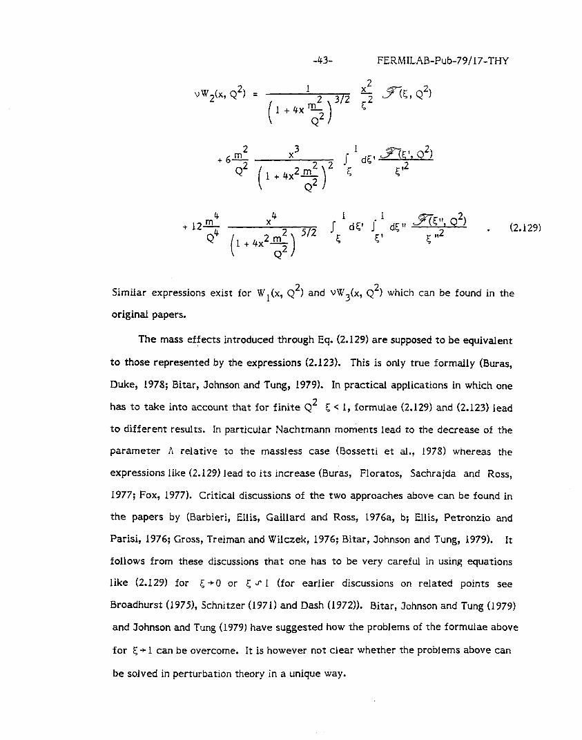
-43- FERMILAB-Pub-79/l-/-THY
vW2(x, Q2) = 1 $ c%C, Q2)
. (2.129)
Similar expressions exist for Wl(x, Q2) and VW3(x, Q2) which can be found in the
original papers.
The mass effects introduced through Eq. (2.129) are supposed to be equivalent
to those represented by the expressions (2.123). This is only true formally (Buras,
Duke, 1978; Bitar, Johnson and Tung, 1979). In practical applications in which one
has to take into account that for finite Q2 5 < 1, formulae (2.129) and (2.123) lead
to different results. In particular Nachtmann moments lead to the decrease of the
parameter A relative to the massless case (Bossetti et al., 1978) whereas the
expressions like (2.129) lead to its increase (Buras, Floratos, Sachrajda and Ross,
1977; Fox, 1977). Critical discussions of the two approaches above can be found in
the papers by (Barbieri, Ellis, Gaillard and Ross, 1976a, b; Ellis, Petronzio and
Parisi, 1976; Gross, Treiman and Wilczek, 1976; Bitar, Johnson and Tung, 1979). It
follows from these discussions that one has to be very careful in using equations
like (2.129) for 5 +O or 5 s 1 (for earlier discussions on related points see
Broadhurst (1975), Schnitzer (1971) and Dash (1972)). Bitar, Johnson and Tung (1979)
and Johnson and Tung (1979) have suggested how the problems of the formulae above
for 5 + 1 can be overcome. It is however not clear whether the problems above can
be solved in perturbation theory in a unique way.
-44- FERMILAB-Pub-79/17-THY
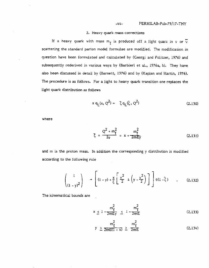
2. Heavy quark mass corrections
If a heavy quark with mass mf is produced off a light quark in v or 7
scattering the standard parton model formulae are modified. The modification in
question have been formulated and calculated by (Georgi and Politzer, 1976) and
subsequently rederived in various ways by (Barbieri et al., 1976a, b). They have
also been discussed in detail by (Barnett, 1976) and by (Kaplan and Martin, 1976).
The procedure is as follows. For a light to heavy quark transition one replaces the
light quark distribution as follows
x qL(x, Q2) + ?S qLc 9 Q2) (2.130)
where
2 Q +m
“5= 5 : 4
= X+2mEy (2.131)
and m is the proton mass. In addition the corresponding y distribution is modified
according to the following rule
( 1
i [ r 2 2
+ (1-y) (1 - yJ2
+;p k y-5 ( ,3 The kinematical bounds are
’ 2 l m: mf 2
-- 2mEy 2 ’ -- 2mE
2 mf m:
y 1 2mE(l - x) 2 m
et1 -i , . (2.132)
(2.133)
(2.134)
-45- FERMILAB-Pub-79/17-THY
from which it follows that the effect of a new quark is seen first at high y and
small x values. In addition since [ > x and qL( 5, Q”) is a decreasing function of F;
the heavy quark contribution is suppressed at all values of x relative to the
contribution of the light-to-light quark transition. Furthermore the y distributions
are distorted relative to the massless case. In summary the full power of the new
contributions due to heavy quark production is expected to be seen only at energies
well above the threshold. For a detailed description of these effects we refer the
reader to papers by (Barnett, 1976), (Kaplan and Martin, 1976) and (Albright and
Shrock, 1977).F21
We have dealt here only with mass effects due to light quark to heavy quark
transitions. The treatment of light or heavy quark production off heavy quarks is
more complicated and can be found in the papers by (Georgi and Poiitzer, 1976) and
(Barbieri, Ellis, Gaillard and Ross, 1976a, b).
E. Structure of Common Asymptotic Freedom Phenomenology
In order to help the reader to use the formulae of this section in
phenomenological applications we present here the structure of common asymp-
totic freedom phenomenology in the form of a recipe. This procedure should be
regarded only as a first try in testing the theory. ‘More fancy ways of confronting
asymptotic freedom predictions with the data are discussed in Sections VI, VII and VIII.
1. Leading order
In the leading order of asymptotic freedom all parton model sum rules and
relations are satisfied. Therefore all known parton model formulae (see Section
1I.B) for deep-inelastic processes are still valid except that now the parton
distributions depend on Q2.
-46- FERMILAB-Pub-79/17-THY
An idealized version of a procedure for testing asymptotic freedom
predictions would be then as follows:
Step 1. Write parton model formulae for all experimentally measured deep-
inelastic processes as ep, up, vN, TIN and in particular consider the quantities <x>,
<Y>, v’w2, u’w3, & and also the moments of structure functions.
Step 2. Collect all existing deep-inelastic data.
Step 3. Choose a value of Q2 = Qz for which perturbation theory makes sense
(say Q:: 2 GeV2, preferably higher) and for which the data are good enough so
that all quark distributions can be found at this value of Q2 for as broad a range in
x as possible.
Step 4. Find qi(x, Qzh
5. Step Choose a gluon distribution G(x, Q$. The shape of the gluon
distribution (e.g. the power of (1 - x)) is not specified directly by the data.
However the second moment n = 2 is fixed by energy-momentum conservation once
the quark distributions are known.
Step 6. Choose A. A good starting point is A= 0.5 GeV.
i) In the moment version: Step 7.
a. calculate< Aij(Q~)>,, <C(Qt)> n, cC(Qz) >,,.
b. calculate < Aij(Q2)>, and CC (Q2) >,, using Eqs. (2.84)-(2.85).
C. calculate the moments of structure functions using formulae of
Section 1I.B.
d. try to include target mass corrections using Nachtmann moments
keeping in mind warnings of Section 1I.D.
ii) In the local version:
a* calculate ‘ij(x, Q:), C(X, Qz) and G(x, Q$ and use them as boundary
conditions to the integro-differential Eqs. (2.52)-(2.54).
-47- FERMILAB-Pub-79/17-THY
b. solve these equations either numerically or by means of approximate
methods discussed in Section V.
C. insert the results for A..(x, Q2), C(x, Q2) in the standard parton ‘J
model formulae (Section I1.B) and calculate various cross-sections and
structure functions.
Step 8. Compare the results of Step 7 with the data. If the agreement is bad,
change a few FORTRAN cards in Steps 5 and 6 and possibly in Step 4.
Check whether fits with various values of Qi give results compatible Step 9.
with each other. This last step can be omitted if the formal Eqs. (2.69b) and (2.74b)
are used.
A few comments are necessary.
or x and y distributions as functions
In calculating the v,; total cross-sections
of energy, one has to integrate over Q2
essentially in the range from 0 to 2 ME. Since the effective coupling constant -2 2 g (Q ) is large for Q2 < 1 - 2 GeV2 and consequently perturbative methods are
inapplicable one has to make assumptions about the Q2 dependence of the quark
distributions for the low values of Q’. Presumably the best method is to use in this
Q2 range the data itself (Fox, 1978a).Another way to circumvent this problem is to
make cuts in Q2 in the data and consequently calculate the experimental as well as
theoretical cross-sections without including the low range of Q’ where perturbation
theory does not make sense (Buras, 1977).
2. Higher orders
The phenomenology of higher order asymptotic freedom corrections has only
reached an early stage of its development, and, consequently, we make only a few
comments here.
One can either directly compare formulae (2.90a, b) and (2.lOla, b) with the
data or devise methods by means of which the effects of higher order corrections
-48- FERMILAB-Pub-79/17-THY
on the leading order predictions are most clearly seen. A typical example of such a
method is the An scheme proposed by (Bate, 1978) and developed by (Bardeen et al .,
1978). We shall discuss this scheme and its various versions in Section VII and turn
now to a parton model formulation of asymptotic freedom beyond the leading
order.
F. Parton Model Formulae for Higher Order Corrections
We first recall that in the leading order of asymptotic freedom the formulae
for the Q2 development of deep-inelastic structure functions can be found by
means of two simple rules:
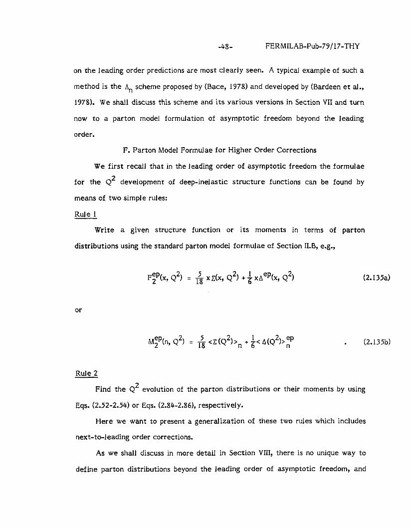
Rule 1
Write a given structure function or its moments in terms of parton
distributions using the standard parton model formulae of Section II.B, e.g.,
2 F;p(x, Q ) = 18 5 x1(x, Q2) + ; xAep(x, Q2)
or
2 M;p(n, Q ) = 18 5 <c (Q2)>, + ;< A(Q2)>zp
(2.135a)
. (2.13533)
Rule 2
Find the Q2 evolution of the parton distributions or their moments by using
Eqs. (2.52-2.54) or Eqs. (2.84-2.861, respectively.
Here we want to present a generalization of these two rules which includes
next-to-leading order corrections.
As we shall discuss in more detail in Section VIII, there is no unique way to
define parton distributions beyond the leading order of asymptotic freedom, and
-49- FERMILAB-Pub-79/17-THY
various definitions are possible. Here we shall present one (Baulieu and Kounnas,
1978; Kodaira and Uematsu, 1978) which is particularly useful in connection with
so-called perturbative QCD (Politzer, 1977a) on which we shall comment in Section
IX.
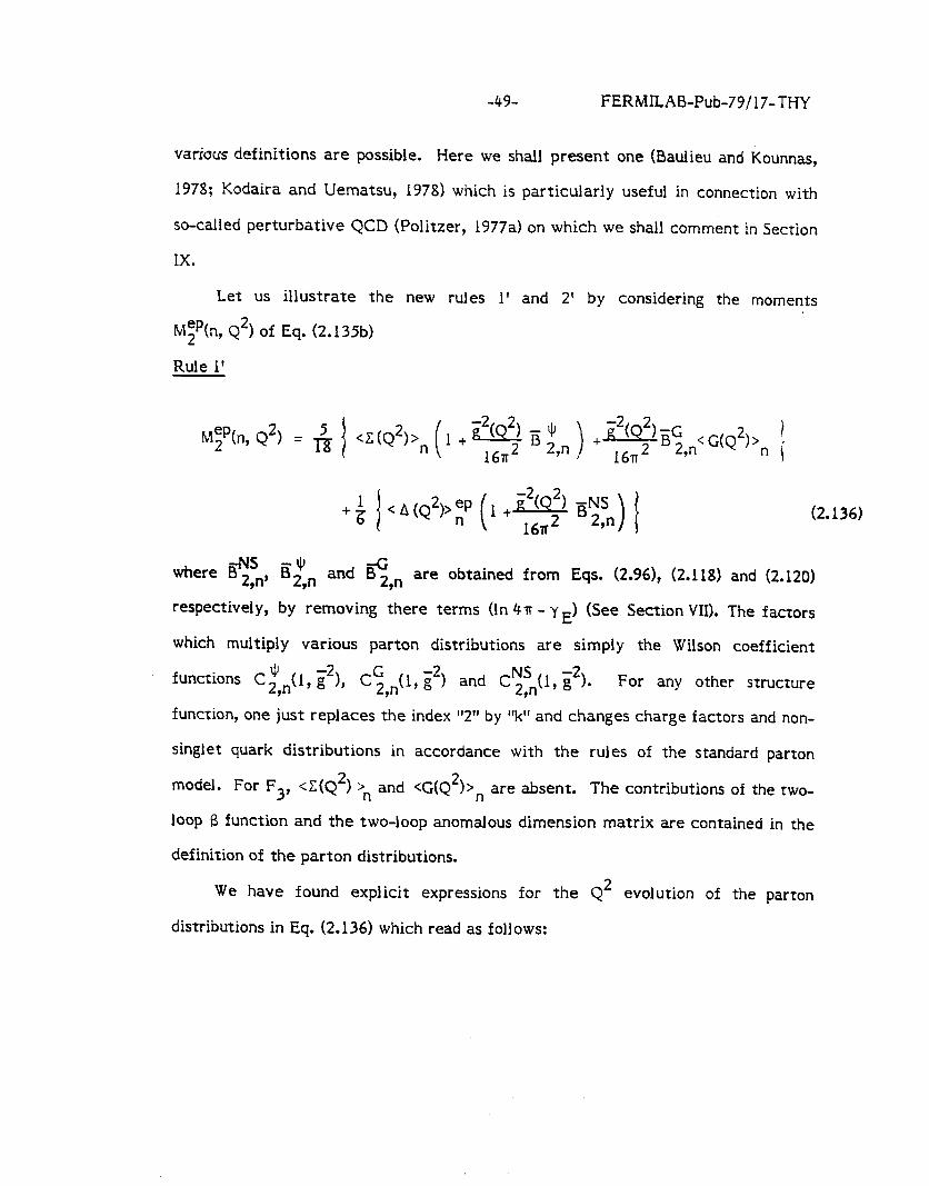
Let us illustrate the new rules 1’ and 2’ by considering the moments
M;p(n, Q2) of Eq. (2.135b)
Rule 1’
M:P(n, Q2) = & 1 <~(Q2bn (1 +-3 B ;,n) +yi;,n<G(Q2)>n 1
+ ; -2 2
1 +a(Q) BySn 16n2 ’
(2.136)
where es sJI -G 2,n’ 2,n and B 2,n are obtained from Eqs. (2.961, (2.118) and (2.120)
respectively, by removing there terms (In ~TF - y E) (See Section VII). The factors
which multiply various parton distributions are simply the Wilson coefficient
functions C&.,(1, g2), C!j .(I, i2) and C:yn(l, z2)* For any other structure 9
function, one just replaces the index “2” by “k” and changes charge factors and non-
singlet quark distributions in accordance with the rules of the standard parton
model. For F3, <C(Q2) >,, and <G(Q’)>, are absent. The contributions of the two-
loop 8 function and the two-loop anomalous dimension matrix are contained in the
definition of the parton distributions.
We have found explicit expressions for the Q2 evolution of the parton
distributions in Eq. (2.136) which read as follows:

-5o- FERMILAB-Pub-79/17-THY
Rule 2’
< Aij(Q2)>, = < A ij(Q4> n d”Ns
f&(Q’, Qz)
d” <c(Q2bn = { (1 - ~,kC (Qf$, - T~,<G(Q$, ) if&& [ 1 +
ij2(Q;, H$ (Q2, Q;)
+ { cr,<C(Q& + En<G(Q&, > = [ 1 4 g2(Q;,
H$(Q’, $1
(2.137)
(2.138)
cC(Q2bn = { an< G(Qz)$, - E~<Z(Q~)>~} ifd d’ HyG(Q2, Q2) [ 1 i2(Q;) 0
d” + i (1 - “,)<G(Q;) ‘,, + cn< C(Q;) >n ) - H_“,(Q’, Qf) (2.139)
where CY n, a,, and cn are given in Eq. (2.87), and dLs and d2 have been defined in
Eqs. (2.70) and (2.77) respectively. Notice similarities with the leading order
expressions (2.84-2.86). The factors H: which include higher order corrections are
given as follows:
HFs(Q2, Qz) = 1 + [z2(Q2) - g2(Q$]
16~2 Gs (2.140)
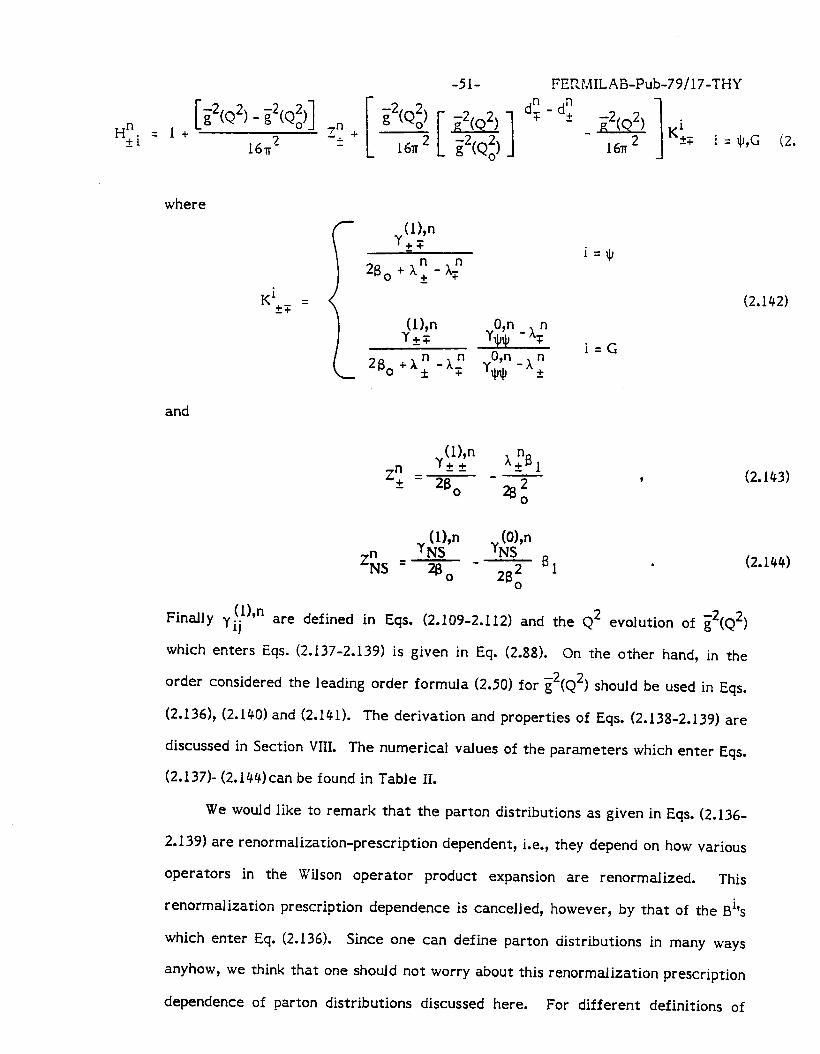
-51- FERMILAB-Pub-79/17-THY
Hyi = l+ [ i2(Q2) - g2(Q2,,]
167~2
where y(l),n +T
28, + x; - A; i- -4J
(2.142)
(1 An YkT
yg - A)
28, +xy -AS” i=G
C
Ki+T =
and
2; = Y!‘$” x “B 2 1 *B - - -
0 a32 0
(2.143)
(2.144)
Finally y :;lPn are defined in Eqs. (2.109-2.112) and the Q2 evolution of g2(Q2)
which enters Eqs. (2.137-2.139) is given in Eq. (2.88). On the other hand, in the
order considered the leading order formula (2.50) for g2(Q2) should be used in Eqs.
(2.1361, (2.140) and (2.141). The derivation and properties of Eqs. (2.138-2.139) are
discussed in Section VIII. The numerical values of the parameters which enter Eqs.
(2.137)- (2.144) can be found in Table II.
We would like to remark that the parton distributions as given in Eqs. (2.136-
2.139) are renormalization-prescription dependent, i.e., they depend on how various
operators in the Wilson operator product expansion are renormalized. This
renormalization prescription dependence is cancelled, however, by that of the Bits
which enter Eq. (2.136). Since one can define parton distributions in many ways
anyhow, we think that one should not worry about this renormalization prescription
dependence of parton distributions discussed here. For different definitions of
-52- FERMILAB-Pub-79/17-THY
parton distributions we refer the reader to the papers by (Altarelli, Ellis and
Martinelli, 1978) and (Floratos, Ross and Sachrajda, 1979). In particular Floratos et
al. present explicit expressions for the Q2 evolution of their parton distributions.
G. Longitudinal Structure Functions
Finally we quote the formula for the longitudinal structure function which we
shall derive in Section VIII. We have
FL(x, Q2) = [F F2(y, Q2) + 6 :)8f(l - ;)y c(~, Q’] (2.144)
where F2(y, Q2) and G(y, Q2) are the full structure functions F2 (singlet +
nonsinglet) and the gluon distribution, respectively. The leading order formulae for
the Q2 evolution of F2(y, Q2) and G(y, Q2) should be used in Eq. (2.144). For f = 4,
df) = 5/18 for ep scattering and J, = 1 for v and J scattering. 42) The
generalizations to arbitary number of flavors are straightforward.
-53- FERMILAB-Pub-79/17-THY
III. QUANTUM CHROMODYNAMICS AND TOOLS TO STUDY IT
In this Section we shall collect certain information about Quantum Chromo-
dynamics (QCD). We shall also present the tools necessary to extract QCD
predictions for deep-inelastic scattering. We shall discuss regularization, renorma-
lization, operator product expansion and renormalization group equations. Our
discussion is mainly devoted to those readers who would like to gain enough
information about these topics to be able to calculate such quantities as the B
function, the anomalous dimensions of quark and gluon fields and the anomalous
dimensions of various operators relevant for the discussion of scaling violations.
Therefore, in our presentation we shall try only to give the reader a feeling for
what is going on-very often by showing examples. We refer the interested reader
to the textbooks (Bogolubov and Shirkov, 1959; Bjorken and Drell, 1965; De Rafael,
1977) and to various oaoers, reviews and lectures (Zimmerman, 1971: Abers and
Lee, 1973: Politzer, 1974; Coleman, 1971: Gross and Wllczek,L973b, 1974;
Abarbanel, 1974: Gross, 1976: Crewther. 1976: Ellis. 1976: Lautrup, 1976; Taylor.
1976: Marciano and Pagels, 19781 where the material of this section is presented in
great depth. This section may be omitted by the experts, without loss of continuity.
A. Lagrangian and Feynman Rules
Quantum Chromodynamics is an SU(3)c color gauge theory which describes
the interactions between quarks and gluons. Quarks are arranged in color triplets
and come in f flavors. The QCD Lagrangian is given by
(3.1)
where a = 1,...8, o, 8 = 1,2,3 and the summation over repeated indices and over fla-
vors is understood. Furthermore
-54- FERMILAB-Pub-79/17-THY
Gd = 2 Ga-a Ga+gfabcGbGc Llv IIV VP P v 9 (3.2)
is the field strength and
(3.3)
is the covariant derivative. $ c1 and G; are fermion and gluon fields respectively.
Finally g is the strong interaction coupling constant. The matrices Xa obey the
commutation relations
[XQq = ifabclc (3.4)
with fabc being the structure constants of SU(3)c. It should be remarked that in
order to specify the theory completely one must add a gauge fixing term to -E4
which for commonly used gauges (covariant gauges) has the form:
-Tr [(auGu)21 /CI, where o is a gauge parameter. In these gauges one must add
Fadeev-Popov ghost interactions to the Lagrangian. In the axial gauge (G; = 0)
there are no ghosts but the calculations of Feynman diagrams are generally more
complicated than in covariant gauges. From (3.1) by means of standard techniques
(e.g. ‘t Hooft, Veltman, 1973; Gross, Wilczek, 1973b) one can derive Feynman rules
which are shown in Fig. 4.
The new features relative to Quantum Electrodynamics are
i) SU(3) group factors
ii) existence of the triple and quartic gluon couplings
and
iii) existence of fictitious ghost couplings.
Otherwise the calculations of QCD Feynman diagrams are very similar to the
corresponding QED calculations. The relevant group factors are defined as follows:
-55- FER:,lIL.48-Pub-79/17-THY
6 &C(G) = facd fbCd
S,bT(R) = fXjt,‘~j
For an SU(3) gauge theory with f flavors, as discussed here,
. (3.5)
C*(R) = ; , C(G) = 3 and T(R) = if 9 l (3.6)
To make the phenomenological applications easier, in all expressions presented in
this review, the values of the group theory factors as given by Eq. (3.6) have been
explicitly used.
B. Renormalization and Renormalization Group Equations
As in QED many calculations of QCD Feynman diagrams with one or more
loops lead to divergent results, and renormalizations of various quantities which
enter the calculations (vertices, propagators) are necessary in order to obtain finite
physical answers. There exists a whole machinery for extracting finite physical
answers from perturbation theory, called the Renormalization Program. It consists
of two steps i) regularization and ii) renormalization.
1, Dimensional regularization
The first step in any renormalization program is to identify the singularities
of a given Feynman diagram and extract them in such a way that renormalization
can be easily performed. One can achieve this in many ways, but a particularly
elegant and simple method is the dimensional regularization procedure of (‘t Hooft
and Veltman, 1972)F22 In which Feynman diagrams are evaluated in D=4-e
dimensions and singularities are extracted as poles: l/c, l/c2, etc.
Let us illustrate this method with a simple example. Consider the one-loop
diagram of Fig. 5a. It represents the virtual gluon correction to the quark
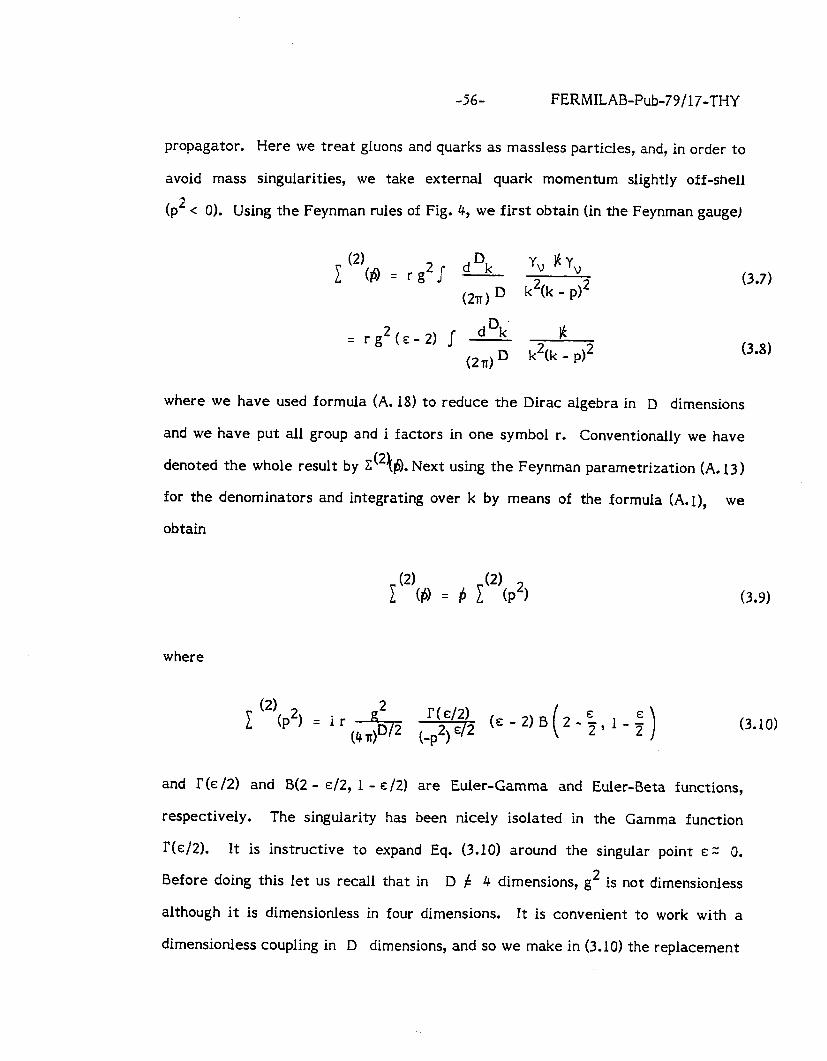
-56- FERMILAB-Pub-79/17-THY
propagator. Here we treat gluons and quarks as massless particles, and, in order to
avoid mass singularities, we take external quark momentum slightly off-shell
(pi < 0). Using the Feynman rules of Fig. 4, we first obtain (in the Feynman gauge)
1 (2)(8 = r g2 J d Dk ‘v Ib ‘v (2nr) D k2(k - p12
= rg2(,-21 J - dDk. Ic (2n) D k2(k - pJ2
(3.7)
(3.8)
where we have used formula (A. 18) to reduce the Dirac algebra in D dimensions
and we have put all group and i factors in one symbol r. Conventionally we have
denoted the whole result by C (2\h). N t ex using the Feynman parametrization (A. 13)
for the denominators and integrating over k by means of the formula (A.l), we
obtain
where
(3.9)
and r(e/2) and B(2 - c/2, 1 - E /2) are Euler-Gamma and Euler-Beta functions,
respectively. The singularity has been nicely isolated in the Gamma function
l?(~/2). It is instructive to expand Eq. (3.10) around the singular point E z 0.
Before doing this let us recall that in D f 4 dimensions, g2 is not dimensionless
although it is dimensionless in four dimensions. It is convenient to work with a
dimensionless coupling in D dimensions, and so we make in (3.10) the replacement
(3.10)
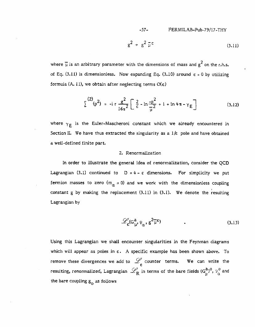
-57-
g2 -P g2 p
FERMILAB-Pub-79/17-THY
(3.11)
where 1 is an arbitrary parameter with the dimensions of mass and g2 on the r.h.s.
of Eq. (3.11) is dimensionless. Now expanding Eq. (3.10) around E: = 0 by utilizing
formula (A. 111, we obtain after neglecting terms O(E)
(2) 1 (p2) = -ir_gL[$-ln$+l+ln4n-~E]
16n2 (3.12)
where yE is the Euler-Mascheroni constant which we already encountered in
Section II. We have thus extracted the singularity as a l/c pole and have obtained
a well-defined finite part.
2. Renormalization
In order to illustrate the general idea of renormalization, consider the QCD
Lagrangian (3.1) continued to D = 4 - E: dimensions. For simplicity we put
fermion masses to zero (mo = 0) and we work with the dimensionless coupling
constant g by making the replacement (3.11) in (3.1). We denote the resulting
Lagr angian by
. (3.13)
Using this Lagrangian we shall encounter singularities in the Feynman diagrams
which will appear as poles in E. A specific example has been shown above. To
remove these divergences we add to 9 counter terms. We can write the E
resulting, renormalized, Lagrangian pR in terms of the bare fields (Gz)‘, ‘4: and
the bare coupling go as follows
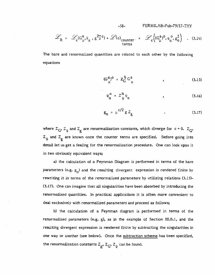
-58- FERMILAB-Pub-79/17-THY
The bare and renormalized quantities are related to each other by the following
equations
(3.15)
(3.16)
(3.17)
where +, J, 2 and Zg are renormalization constants, which diverge for E + 0. ZG,
Z9 and Zg are known once the counter terms are specified. Before going into
detail let us get a feeling for the renormalization procedure. One can look upon it
in two obviously equivalent ways;
a) the calculation of a Feynman Diagram is performed in terms of the bare
parameters (e.g. go) and the resulting divergent expression is rendered finite by
rewriting it in terms of the renormalized parameters by utilizing relations (3.15)-
(3.17). One can imagine that all singularities have been absorbed by introducing the
renormalized quantities. In practical applications it is often more convenient to
deal exclusively with renormalized parameters and proceed as follows;
b) the calculation of a Feynman diagram is performed in terms of the
renormalized parameters (e.g. g), as in the example of Section III.B.1, and the
resulting divergent expression is rendered finite by subtracting the singularities in
one way or another (see below). Once the subtraction scheme has been specified,
the renormalization constants Zg, z G9 Z3, can be found.
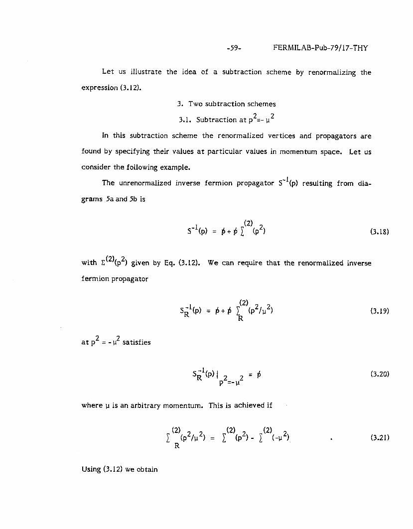
-59- FERMILAB-Pub-79/17-THY
Let us illustrate the idea of a subtraction scheme by renormalizing the
expression (3.12).
3. Two subtraction schemes
3.1. Subtraction at p2=- u2
In this subtraction scheme the renormalized vertices and propagators are
found by specifying their values at particular values in momentum space. Let us
consider the following example.
The unrenormalized inverse fermion propagator S-‘(p) resulting from dia-
grams 5a and 5b is
s-1(p) = h + h 1 (2)
(P2) (3.18)
with C(2)(p2) given by Eq. (3.12). We can require that the renormalized inverse
f ermion propagator
(2) S$P) = b + h lR (P2/u2)
at p2 = - u2 satisfies
S$P) 1 p2,q2
=6
where u is an arbitrary momentum. This is achieved if
1 (2)(p2,u2J = l(2)(P2) - 1(2)(-112) R
(3.19)
(3.20)
(3.21)
Using (3.12) we obtain
-6O- FERMILAB-Pub-79/17-THY
(2) lR (P2/u2) = irg2lnd
161~~ u2
Next writing
S$P) = Z$Sl(P)
we obtain from (3.181, (3.191, (3.12) and (3.22)
.
ZJ, q l+ir$[$-1t-i” T2
+ 1 +ln4n -yE 1 .
(3.22)
(3.23)
3.2. ‘t Hooft’s minimal subtraction scheme
The method presented above is not the only way to render S-‘(p) finite. By
putting condition (3.20) we have subtracted from C (2) 2 (p ) not only the singularity
I/E but also the finite terms. The subtraction procedure in which one subtracts
only the singularity l/c is called minimal subtraction scheme (MS) and has been
proposed by (‘t Hooft, 1973). Applying this procedure to Eq. (3.12) we obtain
(3.24)
2
MS In%-l-ln4r+yE
u2 1 and
zJll - l+ir-$ f MS -
(3.25)
(3.26)
Notice that the expression for the renormalization constant ZQ is very simple in
‘t Hooft’s scheme. Generally in the scheme in question any renormalization
constant is just a series of powers of l/c which greatly facilitates the calculations
of various renormalization group parameters; in particular the calculation of two-
loop anomalous dimensions (for a discussion see Section 3 of Ross, 1979). Notice
-6 I- FERMILAB-Pub-79 /17-THY
that Xg’ is different in the two renormalization schemes considered. This does not
(2) bother us, however, because Ci is not a physical quantity. cp is, in fact,
generally only one element of a physical expression. There are other elements in a
given physical expression which also depend on renormalization procedure. If all
these elements are put together, their renormalization prescription dependences
cancel each other as required for a physical quantity (Stuekelberg and Peterman,
1953). Specific examples of such situations, relevant for deep-inelastic scattering,
will be discussed in Section VII.
Our discussion of It Hooft’s minimal subtraction scheme was very superficial,
Full exposition of this elegant subtraction procedure can be found in the papers by
(‘t Hooft, 1973; Collins and Macfarlane, 1974; Gross, 1976). In particular Collins
and Macfarlane discuss a whole class of subtraction schemes which differ from the
one presented here by a different continuation of the renormalized coupling
constant to D dimensions. In general instead of (3.11) one can have
g2 + g2.;JEfk, g2)
where f(c, g2) is any function of e which has the property f(0, g2) = 1. Each
different continuation will lead to different finite parts in Eq. (3.25). As we shall
see in Section VII this type of ambiguity in the finite parts can be absorbed in the
definition of the effective coupling constant. In particular ,the MS scheme of
Section VII in which the terms involving (in 4~ -YE) are not present in Eqs. (2.96)
and (2.120) corresponds to
(3.27a)
fk, g2) = 1 -$(in41i-yE) . (3.27b)
-62- FERMILAB-Pub-79/17-THY
4. Renormalization group equations
So far we have shown how to regularize and renormalize Feynman amplitudes.
In the process we have introduced an arbitrary normalization scale 1-1. In the
p2 = u2 subtraction scheme p2 stands for the space-like momentum where we
specify the values of particular Green’s functions. In the ‘t Hooft’s scheme the
u =u in the renormalized expression appeared through the continuation of the
renormalized coupling constant to D = 4 - E dimensions. In both schemes the
value of 1-1 is arbitrary. Certainly the final result of a renormalization procedure
cannot depend on the value of p and any change in u can be compensated by the
change in g and the scales of the fields. This is most elegantly expressed by
renormalization group equations (Stueckelberg and Peterman, 1953; Gell-Mann and
Low, 1954; Bogolubov and Shirkov, 1959; Callan, 1970, 1972; Symanzik, 1970;
Wilson, 19691, which we shall discuss now very briefly.
It is convenient to work with the amputated, renormalized, one-particle (+,NG’
irreducible, proper vertex functions I’ R (pi, g, E) which are (suppressing
arguments) defined as follows
(NJI ,NG) (Nq, ,NG) rR
GR = NF
1 #,o) “nG GR(0,2)
(N&j The renormalized Green functions GR are given by
‘L\ ‘NC ) GR = < 0 IT(JI~...J~~
‘4 G 1.., GNG (0 >
(3.28)
(3.29)
and N JI
and NG stand for the number of external fermion legs and gluon legs
respectively. In this notation
-63- FERMILAB-Pub-79/17-THY
sR -1 z r t270)
R .
Similar expressions (N,/,,NG)
exist for the unrenormalized proper vertex functions
rU (pj, go, E) with all renormalized parameters and fields replaced by the
corresponding bare quantities. Because of (3.15) and (3.16) the proper vertex
functions rp ‘NG) and rFe’NG) are related to each other by
(3.30)
‘N$ ,NG) rR
N+/2 NC/2 (N+,N~) (PjYgY&9]1) = ‘9 ‘G ru (Pj, go, &)
and the limit
lim E+ 0
rppNG)(p., g, & ,p 1 = rp’NG)tp., g,p > J I
exists. ‘% ,NG)
Since ru does not depend on u i.e.
& ru ‘% yNG) = o
Y
we obtain from (3.33) and (3.31) the following renormalization group equations
C a vrii + B(g) 4 - 1 (N&) “J;y,,, (g) - t y,(g) rR = 0 where
Y+(g)= $J & in Z *
(3.31)
(3.32)
(3.33)
(3.34)
(3.35)
-64-
In ZG
and
B(g) = P g
FERMILAB-Pub-79/17-THY
(3.36)
(3.37)
The renormalization group functions y,,,(g), Y,(g) and B (g) depend only on g. yJ, (g)
and yGg) are called anomalous dimensions of the fermion field and gluon field
respectively. B(g) is the well-known function which governs the Q2 evolution of the
effective coupling constant as we shall discuss in more detail below. It should be
remarked that 6(g), y *
(g) and v,(g) depend only on the given theory and not on the
particular Green’s function considered.
We would like to remark that generally the renormalization group equations
(3.34) also involve the derivatives with respect to the masses and the gauge
parameter ~1. In order to simplify the presentation we neglect these derivatives
here. For a careful discussion of the renormalization of the gauge parameter we
refer the reader to Sec. 5.4 of the review by Gross (1976).
Equation (3.34) when combined with the standard dimensional analysis can be
used to relate the vertex functions evaluated at momenta pi to the same vertex
functions evaluated at resealed momenta e’pi. In applications to deep-inelastic
scattering t = In Q2/u 2. One obtains (see e.g. Gross, 1976)
(N+‘NG)(,tp rR i’
g) = r ‘% 9N”)(p itt)) exp R ‘9 1
bt _ 1 ii’t’ dg, N+Y~ (g’)+NG ‘Gtg’) 1 (3.38) Et
B (g’)
where jj(t> is an effective coupling constant which satisfies the following equation
; i(t = 0) = g (3.39)
-65- FERMILAB-Pub-79 /17-THY
and 6 is the physical dimension of rR.
We observe that once y8(g), u,(g) and B(g) are known, and I’R (Np,NG) is
calculated at momenta corresponding to a single value of t, say t = 0, then Eq. (N&)
(3.38) gives us rR at any resealed momenta etpi with t f 0.
that equations like (3.38) will be at the basis of discussions of scaling
predicted in QCD.
We shall see
violations as
5. Calculations of renormalization group functions
We can obtain y+(g) in g2 order by inserting ZJI of Eq. (3.26) into (3.35) with
the result (r = iC2(R) = i4/3)
y+(g) = F! (3.40)
which corresponds to the Feynman gauge (a = 1). In an arbitrary covariant gauge a
the result of Eq. (3.40) is to be multiplied by ~1. Alternatively we can calculate
c&O) ys (g) by using renormalization group Eq. (3.34). We insert Sii 2 rR as given by
Eqs. (3.19) and (3.25) into renormalization group equations and compare the powers
of g? Since the g2 expansion of B(g) begins with g3, 8 (g) can be dropped on the
r.h.s. of Eq. (3.34) if we are interested in y(g) in order g2. Therefore we obtain
first
C a pFp - 2 yQ(g)] rfy”) = 0
and consequently (in g2 order)
(3.41)
(3.42)
which by Eq. (3.22) or (3.25) leads to the previous result (3.40).
-66- FERMILAB-Pub-79/17-THY
Similarly one can calculate the anomalous dimension of the giuon field, UC(g),
by considering the diagrams of Fig. 6, with the result (Politzer, 1974; Gross and
Wilczek, 1973)
yG(g) = - g2 161~~ C (3.43)
where r is the gauge parameter.
In order to evaluate B(g) to order g3 one considers either the diagrams of Fig.
7a or the diagrams of Fig. 7b. If the resulting renormalized vertex functions are +0,31
R and $1) respectively then the equations for i3 (g) which follow from
renormalization group Eq. (3.34) are
- B(g) = - -$ cy,f(O’,,,,) .,,:I
B(g) = - -$ [u&f(2J)( 5) + 2+$ + Yl ]
(3.44a)
(3.44b)
where f (“‘3\p2/u2) and f(2’1){p2/u2) are defined as follows
rR (093) = g +
and
(3.45a)
(3.455) rR (291) = g + _B f(2,1) E1
16a2 ( 1 P2 --.- ._
Evaluating ff,s) and $zT1’ (Politzer, 1973; Gross and Wilczek, 1973) and using
(3.40) and (3.43) one obtains from both (3.44a) and (3.44b)
where
-67-
B(g) q -bo-$
FERMILAB-Pub-79/17-THY
B, = ll-ff .
(3.46)
(3.47)
The fact that the coefficient of g3 is negative (for f 2 16) has a very important
consequence-asymptotic freedom. Inserting (3.46) into (3.39) and choosing
t = In Q2/p2, as an example, we obtain
(3.48)
where we have introduced the parameter A which is related to u2 and i2( u2) = g2
by Eq. (2.51). For Q2 + CD this coupling constant which measures the effective
interaction between quarks and gluons at momentum scale Q decreases to zero.
This is what we mean by asymptotic freedom. As we shall see in subsequent
sections the smallness of g2(Q2) for sufficiently large Q2 will allow us to calculate
many quantities in perturbation theory in g2(Q2). This spectacular property is a
special property of non-abelian gauge theories. F23
b So far we have discussed renormalization, renormalization group equations
and asymptotic freedom in general. Before showing how these ideas can be used in
the study of deep-inelastic scattering we have to discuss operator product
expansion.
-6% FERMILAB-Pub-79/17-THY
C. Operator Product Expansion
The basic object in any discussion of deep-inelastic scattering is the spin
averaged amplitude T TV for the forward scattering of a current Jp off a hadronic
state 1 p>. Here J I-r stands either for the electromagnetic current (ep, up
scattering) or a weak current (v,; scattering). We first introduce the operator
T pv =
i I d4z eiq l ‘TO,, (z)$(O))
which is related to T I.lv by
T,, v(Q2f V) = ‘P I ‘,,v 1 P ‘spin averaged
(3.49)
(3.50)
Next the amplitude Tpv(Q2, v) can be decomposed into invariant amplitudes as
follows
T,JQ2, v) = e,,yrL(Q2,v) + dVvT2(Q2,v) -i c paqS - PvaB v T,(Q’, v) (3.51)
with v = p= q and Q2 = -q*. The tensors e and d PV PV
are defined in Eqs. (2.2) and
(2.3).
Following (Wilson, 1969) we can expand the product of currents, which enters
Eq. (3.491, as a sum of products of local operators 0. Lq”‘Pn
I of definite spin n times
certain coefficient functions Ci The index i stands for the type of operator and
will be specified below. In what follows we shall only consider so-called twist
(twist E dimension - spin) two operators which give the &minant
contributions to the moments of the structure functions in the Bjorken limit. The
-6$ FERMILAB-Pub-79/17-THY
higher twist operators are suppressed relative to twist two operators by powers in
Q2. At not too large values of Q2 they are expected (De Rujula, Georgi, Poiitzer,
1977a, b; Gottlieb,l978) to be of some importance only for x close to 1.
The operator product expansion for T is as follows lJV
( quqv
+ g,v- q2 ) qplqp2C1Ln * ($d2)
Writing next
‘Pl’i I-ll4,
Ip > = AL(u2)p ul...pu, - traces
and combining Eqs. (3.50)-(3.53) we obtain
T,,(Q’,v) =
(3.52)
(3.53)
(3.541
-7o- FERMILAB-Pub-79/17-THY
where x is the Bjorken variable (Q*/~v). In writing (3.54) we have dropped the
trace terms of Eq. (3.53). This is justified if target mass corrections (see Section
1I.D) can be neglected. The arguments of the coefficient functions indicate that
they will be calculated in perturbation theory in g2. The sum on the r.h.s. of Eq.
(3.54) runs over spin n, twist 2 operators such as
P 1”‘Pn ‘NS, K
P’1 a*. lJn
OIL = S’TaY p l=!#*...#n $I a- traces)
1-11 . . . Pn
OG = s(GkwJ7p*emefpn-l GpnV _ traces)
(3.55)
(3.56)
(3.57)
where S denotes symmetrization over all Lorentz indices. Since we shall deal only
with foward spin-averaged matrix elements we do not consider operators with
negative parity. u y.4,
ON5 are the fermion non-singlet (under physical symmetries)
operators whereas 0 +I+.) and o Py’~n IJ G are singlet fermion and gluon operators
respectively. The index K distinguishes between various non-singlet operators.
Since the Q* dependence of the Wilson coefficient functions, corresponding to
various non-singlet operators, is common we shall in the following drop the index K.
Using dispersion relations between deep-inelastic structure functions of Eq.
(2.1) and the invariant amplitudes of Eq. (3.511, and taking into account (3.54) one
can express the moments of the structure functions in terms of the Wilson
coefficient functions and the hadronic matrix elements of various local operators.
One obtains (Christ, Hasslacher, Mueller, 1972)
dx x”-*Fk(x, Q*) = I: k = 2,L 0 i
(3.58)
-71- FERMILAB-Pub-79/17-THY
and
s1 cjx x”-lF3(x, Q*) = 1 Aiu2)Ci3n . 0 i
(3.59)
Notice that by taking moments the operator product expansion has been projected
on a given spin; the (n - 2) moment of the structure function depends only on
operators of spin n. Since there are at most .three types of leading operators of a
given spin (Eqs. (3.55-3.57)) the theoretical analysis of QCD predictions for deep-
inelastic scattering is most conveniently done in terms of the moments of various
structure functions rather than in terms of structure functions themselves.
A few final remarks about operator product expansion (OPE) are necessary.
The matrix elements Ain depend on the target ) p>, and are uncalculable in
perturbation theory if the target is a composite object as for instance the proton.
The coefficient functions on the other hand do not depend on the target since they
are determined by the expansion (3.52). They can be calculated in perturbation
theory. In fact what OPE does for us is to separate perturbatively calculable
pieces (coefficient functions) in the expression for the moments of structure
functions from non-perturbative pieces-matrix elements of local operators. A
brief discussion on this factorization in the framework of the perturbative QCD can
be found in Section IX.
We shall now show that the Q* dependence of the coefficient function is
governed by the renormalization group equations similar to Eq. (3.34).
-72- FERMILAB-Pub-79/17-THY
D. Renormalization Group Equations for Wilson Coefficient Functions
We begin the discussion with the coefficient functions of the non-singlet
operators of Eq. (3.55). Suppressing for simplicity all the arguments, we write the
non-singlet part of the operator product expansion of two currents symbolically as
follows
JJ I NS = InNS ’ cNSon n
Sandwiching Eq. (3.60) between non-singlet (quark) states we obtain
<NSIJJ/NS> = 1 C;sO;sNS n 9
where
<NS lOis INS > = O;s,Ns .
(3.60)
(3.61)
(3.62)
In order to derive renormalization group equations for C:‘, we have to find first
renormalization group equations for < NS 1 JJI NS > and O& 9 NS.
ForcNS(JJ(NS > we have similarly to Eq. (3.34)
[ a
paFt + tw & -*y+(g) 1 <NS IJJ(NS> = o (3.63)
where y +
(g) is the anomalous dimension of the quark field (see Eq. 3.40). Due to
current conservation, the anomalous dimension of the current J is zero.
Next we define the wave function renormalization 2& of the operator Ois
bY
-73- 04
ONS o& = - GS
FERMILAB-Pub-79/17-THY
(3.64)
where Oiin is the bare operator.
For the matrix element O\s,Ns we therefore have
‘Q On ‘\S NS = n 9 OFiS NS
‘NS ’ (3.65)
with Z,,, defined by Eq. (3.16).
Repeating the steps which led us from Eq. (3.31) to Eq. (3.34) we obtain
1 O"NS,NS = '
where
(3.66)
(3.67)
is the anomalous dimension of the operator Ohs. Next combining Eqs. (3.611, (3.63)
and (3.66) and taking into account that the tensor structure in the expansion (3.60)
is different for different n (see Eq. 3.52), we finally obtain for each n
,g+;s($*) = 0 ’ (3.68)
Notice that we have now written explicitly the arguments of the coefficient
functions.
The case of singlet operators 0; and 0: is more complicated because these
operators mix under renormalization and Eq. (3.64) is replaced by
-74- FERMILAB-Pub-79/17-THY
0; = 1 ( q ab oflt” b
a,b = $,G
Here (2” -1
) is a 2 X 2 matrix. Consequently, Eq. (3.65) is generalized to
ozc = Y ,! zc(zn-l ,,,o;‘;
b a,b,c = $,G 9
where
OiC 9 g <clo;lc>
. (3.69)
(3.70)
(3.71)
and zc stands either for 2 or ZG 9 which are defined in Eqs. (3.16) and (3.17),
respectively. Therefore we have
1 0; c = 0 Y (3.72)
where y n ab are the elements of the 2x 2 anomalous dimension matrix and are
defined by
Equations (3.61) and (3.63) are generalized to the singlet case as follows:
<cjJJlc>= 1 C”,O;, n,b 7 ,
(3.73)
(3.74)
and
-75- FERMILAB-Pub-79/17-THY
C B(g)& - *y,“(g) 1 r: ($0; c = 0 . b Y (3.75)
Therefore, combining Eqs. (3.72) and (3.75) we finally obtain
. (3.76)
Equations (3.66) and (3.75) are the basic results of this Section. We shall
discuss the solutions of these equations in Sections IV, VII and VIII, and now we turn
to the calculation of the anomalous dimensions yis and y ib.
E. Calculations of Anomalous Dimensions of Local Operators
We first write the perturbative expansions of the matrix elements Ois NS
and Oi,cy dropping p* independent terms, as follows Y
O;sNS = Y + O(g4)
and
oEc = 6,,c+ Y
Y (3.77)
(3.78)
where rLs and r” bc are calculable numbers and p* is the space-like momentum of
the quark or gluon states (NS, C) between which the operators are sandwiched.
Furthermore, the perturbative expansions of y:,-(g) and y:b(g) are
2 y;,(g) = yNS 16r2 Opn A- + O(g4) (3.79)
and
-76- FERMILAB-Pub-79/17-THY
2
y:(g) = Yab 16a2 Oyn -a- + O(g4) . (3.80)
Inserting Eqs. (3.77) through (3.80) into Eqs. (3.66) and (3.72) and choosing 4
different combinations of a and c in Eq. (3.72), we obtain the following relations
between the coefficients of In -p*/p* in Eqs. (3.77) and (3.78) and the anomalous
dimensions of the operators
y&J = r&+*y,i
04 yab = ‘ab n + *Yzsab a,b = $,G .
(3.81)
(3.82)
Here yz stands for either yi or yl which are defined in Eqs. (3.40) and (3.43),
respectively.
It follows from (3.81) and (3.82) that in order to find yi;” and yz, we have
to calculate the matrix elements of local operators sandwiched between quark and
gluon states and pick out the coefficients of In -p*. For diagonal elements y 8
yNS Oyn and yc”;;” we have to add, in addition, twice the anomalous dimensions of the
quark and gluon fields which we have already calculated earlier.
The diagrams which enter the calculation of yiGn or yikn are shown in Fig. 8.
The diagrams which enter the calculation of the whole anomalous dimension matrix
in order g2 are shown in Fig. 10. The virtuai gluon corrections on the external lines
need not be calculated if 2y,z or 2~: is added explicitly as in Eqs. (3.81) and (3.82).
On the other hand, if these diagrams are included in the calculations, the
anomalous dimensions y ’ $
and yl should be dropped in Eqs. (3.81) and (3.82).
In order to evaluate the diagrams of Figs. 8 and 10 we have to extend the list
of Feynman rules of Fig. 4 by the rules for the vertices “x” which represent
operator insertions into a two-point function. Simple rules for the vertices in
-77- FERMILAB-Pub-79/17-THY
question have been found by (Gross and Wilczek, 1974) and are shown in Fig. 9. The
A ~ appearing there is an arbitrary four vector with the property
A2 = 0 . (3.83)
The derivation of these rules can be found in the appendix of the paper by Gross
and Wil czek. Additional rules necessary for the calculation of the anomalous
dimensions in order g4 can be found in the paper by (Floratos, Ross and Sachrajda,
1979). Here we shall only indicate how to reproduce formula (2.79a) for y 04 w’
We begin with the diagram of Fig. 8b. We work in the Feynman gaugeF24 and ob-
tain first
Ib = hs dDk Y, lG& Y,
(2tr)D (k*)2k - p)* (A k)“-1
h&2)1* w = (*ldD (k *)*(k _ p)* (Ak)“-’ (3.84)
where we have used formula (A.20) to- reduce the Dirac algebra in D dimensions
and we have put all group and i factors in one symbol h. Now as the reader may
convince herself (himself), if we are interested only in the coefficients of In p*, we
can put c = 0 at all places where this substitution does not lead to a singularity.
From this it follows (see below) that, equivalently, anomalous dimensions can be
found by calculating the coefficients of the divergent parts l/c. On the other
hand, if we are interested in the calculations of the so-called constant pieces (e.g.
1 + In ~JT - yE in Eq. 3.12) we have to keep all E factors different from zero until
the calculation is finished. In particular the “1,’ in Eq. (3.12) comes from the
product of c in (Eq. 3.8) and the divergence l/c in I’(&/*).
-78- FERMILAB-Pub-79/17-THY
Using the formulae of Appendix A, Eqs. (3.11), (3.83) and h= -iC2(R) with
C*(R) given by (3.6), we obtain
2 2 7 -InA
P2 1 aCtA p)“-’ + const . (3.85)
The factor (Ap)“-1 in Eq. (3.85) arises in the following way. After using the
Feynman parametrization of Eq. (A.13) one makes a change from k to c:
ii = k-p(l-x)
where x is the Feynman parameter. Therefore one obtains
(Ak)“-’ = (1 - X)nw'fAp)n" + (n - I)(1 - x)"'~~P)"'~& + . . . . (3.86)
The terms which involve more than one factor Al; can be dropped in Eq. (3.86)
because they lead after K integration to A* which is zero. An additional factor c\p
in the second term in Eq. (3.86) is obtained after ‘k integration, when Eq. (3.86) is
inserted into (3.84).
Adding zeroes order contribution ( [ 1 ] & dp)“-1) to Iby and comparing the
result with Eq. (3.78) and taking into account (3.81), we obtain the following
contribution of diagram 8b to y 04 Jnl,:
4C+R) - Iii (3.87)
Notice that result (3.87) could also be read off the coefficient of l/~. This is
particularly useful in the calculation of two-loop anomalous dimensions as discussed
in detail by (Floratos et al., 1977, 1979).
-79- FERMILAB-Pub-79/17-THY
The diagrams 8a and 8c give the following contribution to y g :
n 1 8C2(R) 1 7
j=* J (3.88)
and when the result for 2y” = *C*(R) is added to Eqs. (3.87) and (3.88), 9
we obtain
W y*9
= 2C2(R) 1 - n& + 4 i c j=* 1 1
(3.89)
*
which by Eq. (3.6) for C*(R) agrees with (2.79a). The calculation of the remaining
elements of the anomalous dimension matrix proceeds in a similar way.
-8O- FERMIL,43-Pub-79/17-THY
IV. Q* DEPENDENCE OF THE MOMENTS OF STRUCTURE FUNCTIONS IN ASYMPTOTICALLY FREE GAUGE THEORIES
A. Preliminaries .
In this section we shall find the Q* dependence of deep-inelastic structure
functions as predicted by asymptotic freedom in the leading order. The basic
formulae of this section (4.17, 4.18, 4.41) express the moments of structure
functions in terms of unknown (Q’ independent) matrix elements of certain
operators times their coefficient functions with explicit Q* dependence. In the
next section we shall cast formulae (4.17, 4.18, 4.41) into the standard parton
model expressions with Q* dependent quark distributions. The reason for a careful
discussion of structure functions in terms of Wilson coefficient functions first
rather than immediately in terms of parton distributions is that beyond the leading
order the definition of parton distributions is not unambiguous and the language
developed in this section is more appropriate. This section is slightly formal but we
invite the reader to go through it carefully since the techniques presented here will
be at the basis of Sections VII and VIII.
As we saw in Section III, the basic tools necessary to study QCD implications
for deep-inelastic scattering are the Wilson operator product expansion and the
renormalization group equations. The operator product expansion allowed us to
systematically identify the dominant contributions to the moments of the structure
functions at large Q* and to express them in terms of a sum of products of
(perturbatively) calculable coefficient functions and (by present methods) uncalcu-
lable matrix elements of certain operators between hadronic states. The Q*
dependence of the coefficient functions could then be found by means of
renormalization group equations. Explicitly we have
0 dx x”-*FL(x, Q*) = 1 A;(p*)C’
i L,n($yg2) (4.1)
-81- FERMILAB-Pub-79/17-THY
dx x”-*F2(x, Q*) q 1 A;(!J*)+ ‘)
(4.2) 0 i
and
dx x n-1F3(x, Q*) q ANS (3)~“’ d
0 n 3,n( u2 y g2) (4.3)
where the sum runs over spin n, twist 2 operators such as the fermion non-singlet
operator Ois and the singlet fermion and gluon operators 0; and O& respectively.
The A’,(u*), which are independent of Q*, are the reduced hadronic matrix
elements of the operators in question. They are defined in Eq. (2.63). We have
shown explicitly that A:( u2) depend on ? , the subtraction point (see discussion in
Section III). Notice that to the moments of F3 only one type of operators
contributes. This is explained in Section VI1.E. NS We would like to recall that in our notation On stands for any linear
combination of non-singlet operators which differ from each other by X” in Eq.
(3.55). Therefore as emphasized after Eq. (2.64) &is(u2) depend generally on the
process and the structure function considered. This dependence is discussed in
Appendix B.
We shall now find the explicit Q* dependence of the coefficient functions
C~,,(Q*/u*, g*) as given in the leading order of asymptotic freedom. To this end it
is convenient to decompose any structure function into a sum of singlet and non-
singlet contributions as follows
Fk(x, Q*) = F;‘(x, Q*) + F;(x, Q*) k = L,2,3 . (4.4)
Particular examples of such decomposition in the framework of the simple parton
model are given in Section 1I.B. The moments of the functions FFS and FE are
given as follows
-82- FERMILAB-Pub-79/17-THY
dx xn-2 NS 0
Fk (x, Q*) = AfS(u2)CNS 2 k,n( p2?g2) k=L~2
dx x 0
n-1F3(x, Q*) = A;‘(IJ*)C;‘~ Y
(4.5)
(4.6)
and
il 0
dx x”-*F;(x, Q*) = A;( u*)C; n Y k = 2,L . (4.7
B. Non-Singlet Structure Functions
The Q* dependence of CNS * * * is governed by the following kyn(Q h Y & ) renormalization group equations
L- lJ 8% + B(g) & -Y\S(gJ]c~~n(~Yg2) = O (4.8)
where FNs(g) is the anomalous dimension of the nonsinglet operator O\s and B(g) is
the renormalization group function which governs the Q* dependence of the
effective coupling constant
. (4.9)
Here t = In Q*/u* and g is the renormalized strong interaction coupling constant.
The solution of Eq. (4.8) is given as follows
To proceed further one has to calculate CNS kyntl, i*), Y is(g) and B (g) in perturbation
theory. In the leading order it is enough to calculate one-loop contributions to
Y\S(g,) and B(g’) using the methods of Section II, and take the zero loop (parton
NS model) values for C ,, ,( 1, i*). Thus in the leading order we have
-83- FERMILAB-Pub-79/17-THY
and
B(g) = - 8, A?- 16~r*
I
s 04 k = 2,3 cp;l;n(l, g*) = NS
7 (4.11)
(4.12)
(4.13) [ 0 k=L
where 6ks are constants which depend on weak and electromagnetic charges (see
(O),n Appendix B), and B. and yNs are given in Eqs. (2.49) and (2.71) respectively.
Inserting Eqs. (4.11) to (4.13) into (4.10) and performing the integral we obtain
k*(Q*) d”NS
3 k = 2,3
= i2( P2)
k=L
where
d” NS= 28 0
(4.14)
(4.15)
Now from Eqs. (4.9) and (4.12) we have
i*(Q*) = 16r* . (4.16)
where the scale parameter A is related to p and i*(p*) = g* by Eq. (2.51).
Combining Eqs. (4.5), (4.6), (4.14) and (4.16) we finally obtain
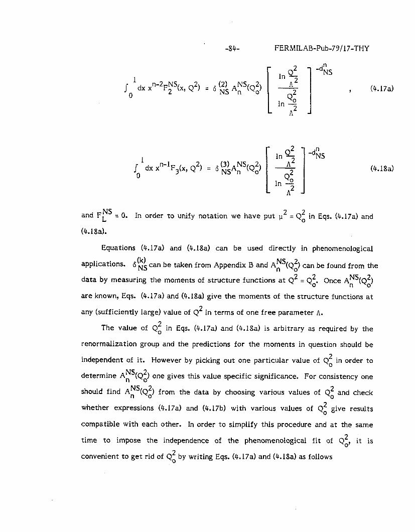
-84- FERMILAB-Pub-79/ 17-THY
-dis
il 0
dx x”-*F;~(x, Q*) = 6 (i’s A;‘(Q;) , (4.17a)
(4.18a) dx x 0
n-1F3(x, Q*) = 6 (ik~fiJS(Qj$ In 5 -dZXS
[ I Q2 In -2
A2
and Frs = 0. In order to unify notation we have put p2 = Qi in Eqs. (4.17a) and
(4.18a).
Equations (4.17a) and (4.18a) can be used directly in phenomenological
applications. 6 (k) NS can be taken from Appendix B and An NstQ;) can be found from the
data by measuring the moments of structure functions at Q2 = Qz. Once Af’(Qz)
are known, Eqs. (4.17a) and (4.18a) give the moments of the structure functions at
any (sufficiently large) value of Q* in terms of one free parameter A.
The value of Qi in Eqs. (4.17a) and (4.18a) is arbitrary as required by the
renormalization group and the predictions for the moments in question should be
independent of it. However by picking out one particular value of Qz in order to
determine Af’(Qz) one gives this value specific significance. For consistency one
should find Af’(Qi) from the data by choosing various values of Qz and check
whether expressions (4.17a) and (4.17b) with various values of Qi give results
compatible with each other. In order to simplify this procedure and at the same
time to impose the independence of the phenomenological fit of Q$ it is
convenient to get rid of Qi by writing Eqs. (4.17a) and (4.18a) as follows
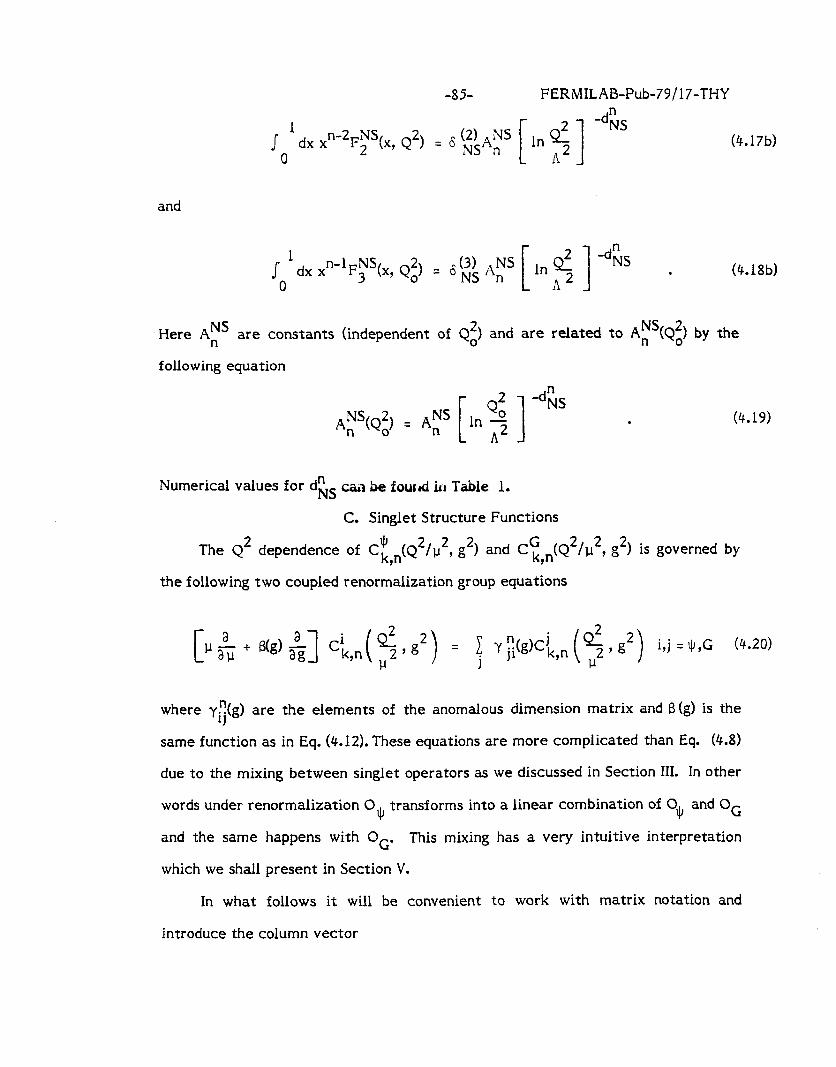
-85- FERMILAB-Pub-79/17-THY
II dx x”-*F~~(x, Q*) q 6 ($AzS -d”Ns
0 (4.17b)
and
j- ’ dx xn-lF~s(X, QE) = 6 E$ A;S ln $ [ 1 0 . (4.18b)
Here ANS n are constants (independent of Qi) and are related to An NS(Qf$ by the
following equation
ANS(Q*) - ANS
n o- n (4.19)
Numerical values for d\S C&I be fowd i.11 Table 1.
C. Singlet Structure Functions
The Q2 dependence of C&,(Q*/u*, g*) and ~&.,(Q*/IJ*P g*) is governed bY
the following two coupled renormalization group equations
[ p&+8(g)&] ct,n($,g2) = 5 y$gJC~,n($,g2) M=W @JO)
where y;(g) are the elements of the anomalous dimension matrix and 8 (g) is the
same function as in Eq. (4.12). These equations are more complicated than Eq. (4.8)
due to the mixing between singlet operators as we discussed in Section III. In other
words under renormalization 0 4J transforms into a linear combination of 0 Q and OC
and the same happens with OG. This mixing has a very intuitive interpretation
which we shall present in Section V.
In what follows it will be convenient to work with matrix notation and
introduce the column vector
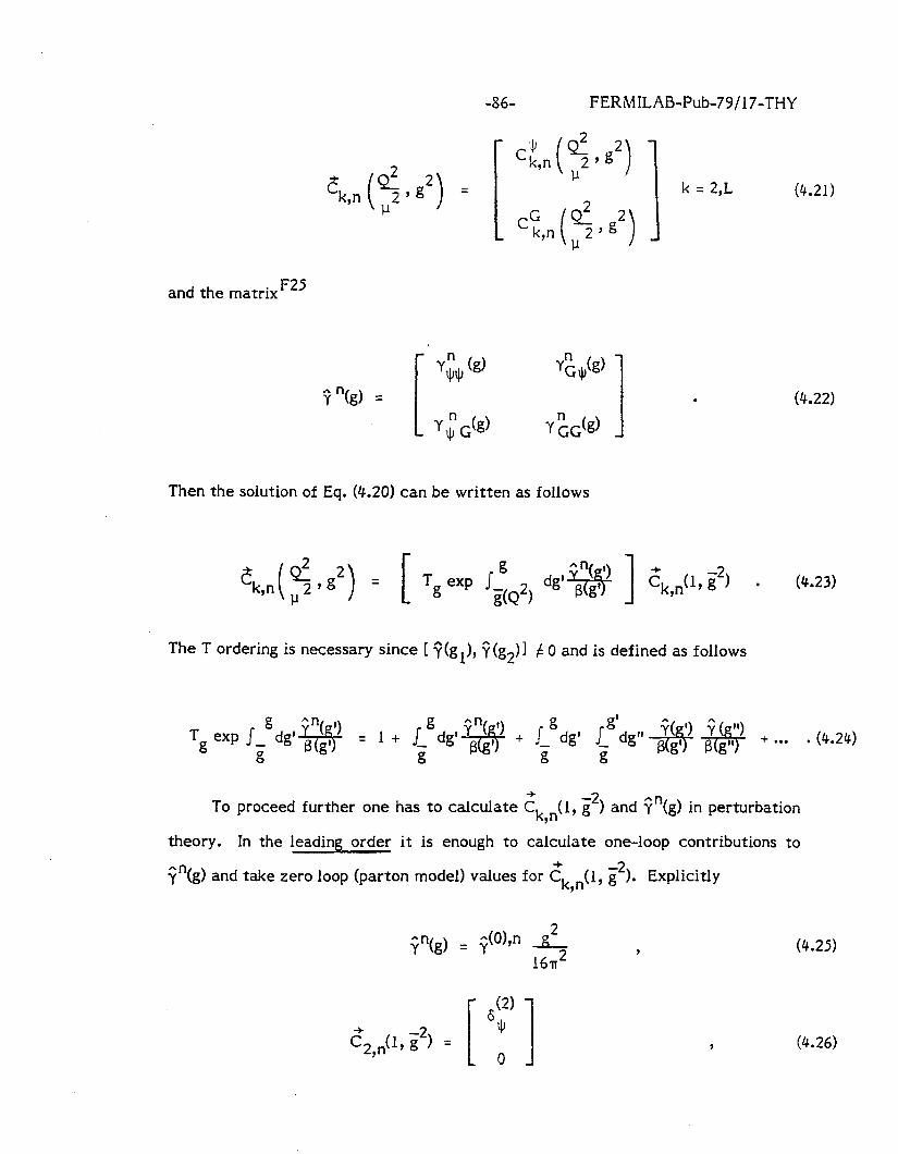
-86- FERMILAB-Pub-79/17-THY
E,,n($2) = and the matrixFz5
y”(g) = 1 . Y ;G(g)
(4.21)
(4.22)
Then the solution of Eq. (4.20) can be written as follows
zk,n ( 5 ) g’ ) = [ Tg exp .fiQ2, dg’@ ] zk,& ii*) . (4.23)
The T ordering is necessary since [ T(g,), y (g,)] f 0 and is defined as follows
Tg exp ,_” dg’$@ = 1 + I_gdg’& + Y-Y 9 J- gdg’ . (4.24) g g g
%‘dgll.#$ -&+ + . . .
To proceed further one has to calculate ck,,(l, i*) and T”(g) in perturbation
theory. In the leading order it is enough to calculate one-loop contributions to
e”(g) and take zero loop (parton model) values for dk,n(l, g*). Explicitly
q”(g) = y -(Oh _gl_ 161~~
(2) [ 1 “Q
0
9 (4.25)
7 (4.26)
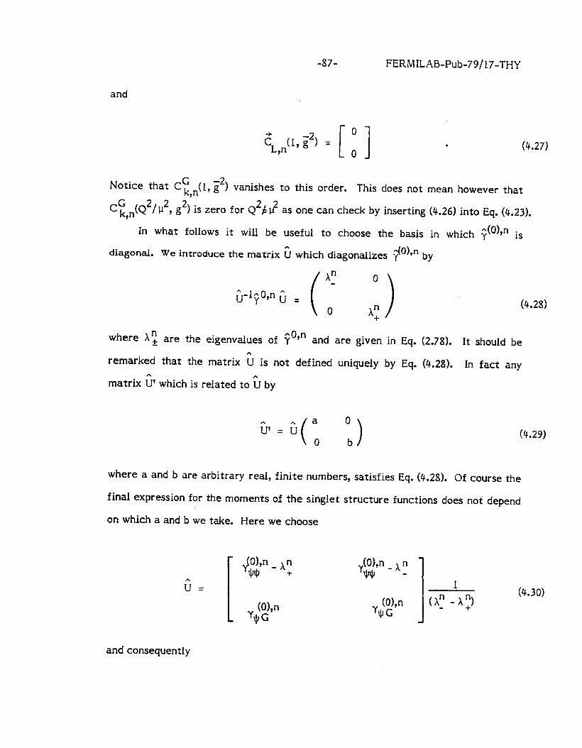
-87- FERMILAB-Pub-79/17-THY
and
EL .(I, g*, = 0
9 [ 1 0 . (4.27)
Notice that CG k,n(l, i*) vanish es to this order. This does not mean however that
C~,n(Q2/u2, g*) is zero for Q2f 3 as one can check by inserting (4.26) into Eq. (4.23).
In what follows it will be useful to choose the basis in which y +O),n is
diagonal. We introduce the matrix 6 which diagonalizes y d”h by
(4.28)
where ht are the eigenvalues of yoyn and are given in Eq. (2.78). It should be
remarked that the matrix ^v is not defined uniquely by Eq. (4.28). In fact any
matrix fit which is related to ^v by
G(“, “,) (4.29)
where a and b are arbitrary real, finite numbers, satisfies Eq. (4.28). Of course the
final expression for the moments of the singlet structure functions does noi depend
on which a and b we take. Here we choose
(Oh _ x n ywJ - 1
J 1
ydodf” 0; -x:1
(4.30)
and consequently
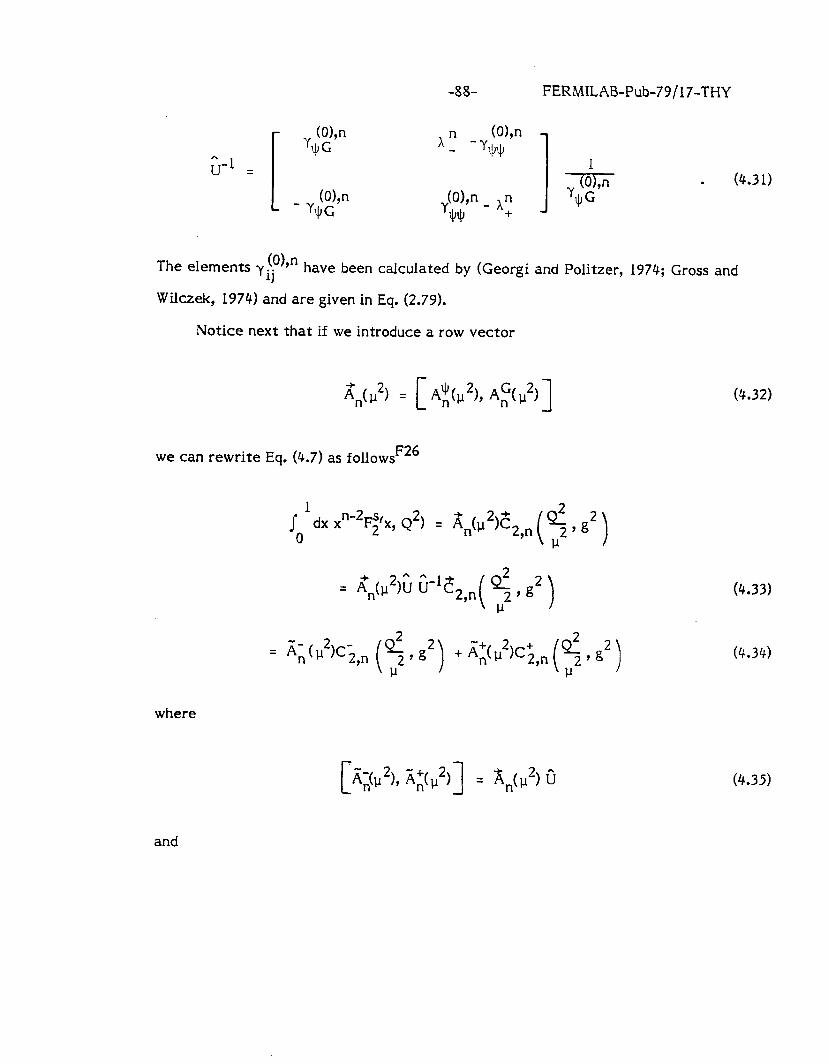
-8% FERMILAB-Pub-79/17-THY
(O),n c
(O),n
;I-’ = -w - Y$lJJ
(4.31) (Oh
- y$G K&n _ xn
3JJI + 1 The elements y . . (Oh
11 have been calculated by (Georgi and Politzer, 1974; Gross and
WiIczek, 1974) and are given in Eq. (2.79).
Notice next that if we introduce a row vector
1 we can rewrite Eq. (4.7) as follows F26
il 0
dx x”-*FTx, Q*) = A&*)? 2,n(s9g2)
where
+ *^ ^-I’ 2 = An(P Iv u C*,n i: ‘1 2’g
(4.32)
(4.33)
(4.34)
(4.35)
and
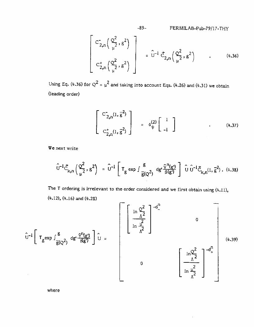
-89- FERMILAB-Pub-79/17-THY
(4.36)
Using Eq. (4.36) for Q* = p2 and taking into account Eqs. (4.26) and (4.31) we obtain
(leading order)
C;7nt’ 7 ii*)
[ I c; $7 ii*) 7
= &2) l 9 [ 3 -1 . (4.37)
We next write
6-1~k7n (5 7 g*) = 2-l [ Tg exp JiQ2, dgl$$$] b c‘1Ek7n(17 g*) l (4.38)
The T ordering is irrelevant to the order considered and we first obtain using (4.111,
(4.121, (4.16) and (4.28)
G-1 g TgexP J- 9 9 dQ*) dF+$- 1 A u=
.l
In OL A2
In J A2
0
-d” -
0
-d:
(4.39)
where
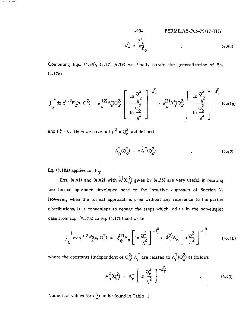
-9o-
A” FERMILAB-Pub-79/17-THY
. (4.40)
Combining Eqs. (4.34), (4.37)-(4.39) we finally obtain the generalization of Eq.
(4.17a)
SO1 dx x”-*F;(x, Q*) = 6 (‘)A;(Q;)
Q
lnQI A2 Q2
In 0 A2
lnQf A2 Q2
In o A2
and F[ = 0. Here we have put p2 = Qz and defined
Eq. (4.18a) applies for F3.
Eqs. (4.41) and (4.42) with ii given by (4.35) are very useful in relating
the formal approach developed here to the intuitive approach of Section V.
However, when the formal approach is used without any reference to the parton
distributions, it is convenient to repeat the steps which led us in the non-singlet
case from Eq. (4.17a) to Eq. (4.17b) and write
-d;
(4.41a)
(4.42)
dx x 0
“-*F;(x, Q*) = $)A; [ln$]-d’+ $?A: [ ins]“:
where the constants (independent of Q:) AZ are related to Az(Q:) as follows
Q2 -d; Az(Qz) = AX In o [ 1 A2
(4.41b)
. (4.43)
Numerical values for d”+ can be found in Table 1.
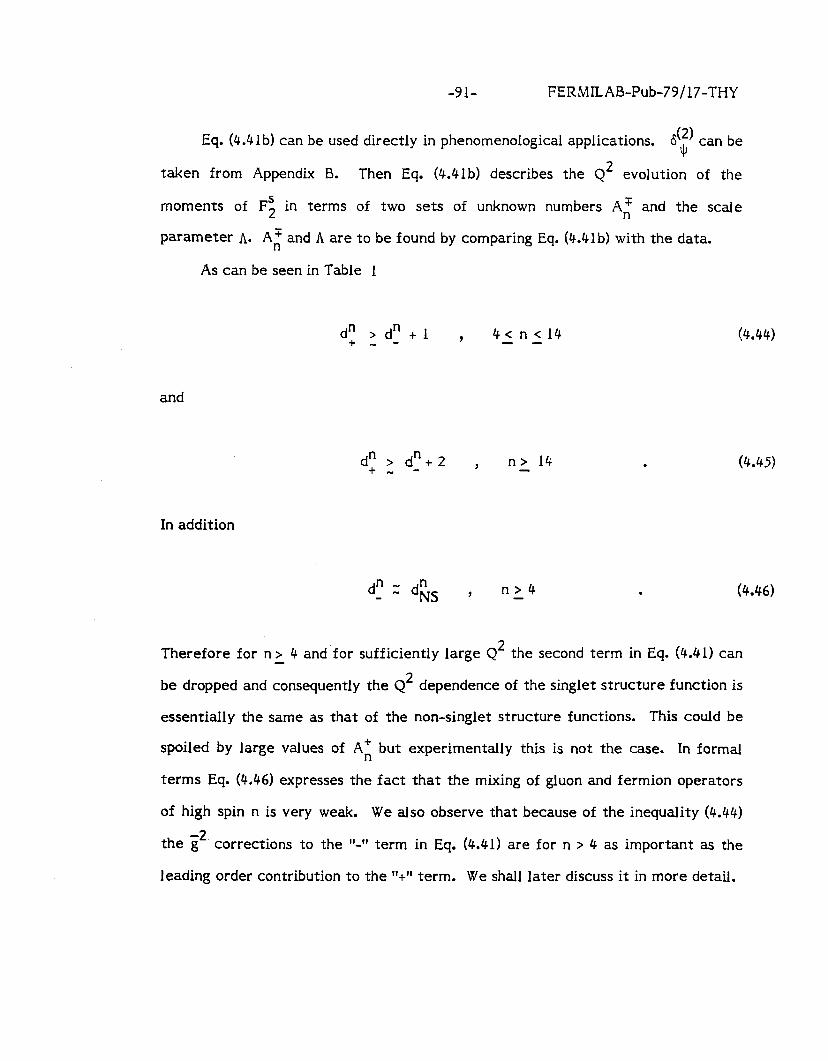
-91- FERMILAB-Pub-79/17-THY
Eq. (4.41b) can be used directly in phenomenological applications. 6(*) can be IJ
taken from Appendix B. Then Eq. (4.41b) describes the QL evolution of the
moments of F; in terms of two sets of unknown numbers AX and the scale
parameter A. AZ and A are to be found by comparing Eq. (4.41b) with the data.
As can be seen in Table 1
d; > d_” +l 7 _ _ 4<n<14
and
d:>d_“+2 , _ n> 14
In addition
d” .., - - d&s 7 - n>4
.
.
(4.44)
(4.45)
Therefore for n > 4 and for sufficiently large Q* the second term in Eq. (4.41) can
be dropped and consequently the Q* dependence of the singlet structure function is
essentially the same as that of the non-singlet structure functions. This could be
spoiled by large values of AA but experimentally this is not the case. In formal
terms Eq. (4.46) expresses the fact that the mixing of gluon and fermion operators
of high spin n is very weak. We also observe that because of the inequality (4.44)
the EL- corrections to the V’ term in Eq. (4.41) are for n > 4 as important as the
leading order contribution to the ‘I+” term. We shall later discuss it in more detail.
-92- FERMILAB-Pub-79/17-THY
V. Q* DEPENDENCE OF PARTON DISTRIBUTIONS IN THE LEADING ORDER
The discussion of the Q* dependence of the structure functions as presented
in Section IV was rather formal and it is useful to develop a more intuitive picture.
In fact, this can be done at least in the leading order. The result is simple and was
already announced in Section II: all well-known par-ton model expressions remain
unchanged except that now parton distributions depend on Q*. Thus if we only find
the Q2 dependence of parton distributions predicted by asymptotic freedom, we can
study QCD effects in deep-inelastic scattering by means of the standard parton
model formulae. The aim of this section is to present equations which determine
the Q2 dependence of parton distributions, solve them and show that they are
equivalent to the formalism developed in Section IV.
A. Intuitive Picture and Integro-differential Equations
We begin with the intuitive picture of (Kogut and Susskind, 1974). Imagine
the photon, 2’ boson or a W boson to be a microscope by means of which we probe
the inner structure of the proton or general1 y of a hadron. Increasing Q2 while
holding x fixed is equivalent to increasing the power of the microscope or looking
at shorter and shorter distances. By scanning the proton at fixed Q* and 0 < x < 1, - -
we obtain the picture of the proton at this particular value of Q*. According to the
simple parton model of Section ILB, the picture of the proton does not depend on
how strong a microscope we use. The pictures at different values of Q* are the
same. This is not the case in QCD. By increasing the power of our microscope
from Q: to Q$ > Q:, we can resolve a quark with momentum fraction x into a
quark with x’ < x and a gluon with x” = x - x1 as illustrated in Figure 3a. Similarly a
gluon with momentum fraction x can be resolved into a quark-antiquark pair as
illustrated in Fig. 3b. There exists also the process of Fig. 3c which can be
-93- FERMILAB-Pub-79/17-THY
interpreted as resolving a gluon into a gluon pair. Since a gluon couples neither to
y nor to Z” or W’, this does not happen directly. However, the existence of this
process affects the probability of finding a quark in a gluon since a gluon can either
fragment into a quark-antiquark pair or into a pair of gluons and the sum of these
two probabilities (plus the probability that the gluon does not fragment at all) is
just unity. In summary the picture of the proton or, equivalently parton
distributions, depend on Q*.
The Q* dependence is different for different parton distributions. Intuitively
valence quarks can effectively only emit gluons. They cannot be produced
effectively in the Fig. 3b process because this would lead to baryon number non-
conservation. As a result, valence quarks lose their momentum in favor of gluons
and consequently (through the process of Fig. 3b) in favor of the sea. In the simple
language developed above, by increasing Q* we cannot find a valence quark in a
gluon or in a sea quark but only in a valence quark itself. Of course this picture is
oversimplified since it assumes one can make a clear distinction between valence
and sea quarks as in Eqs. (2.12) and (2.13).
The behavior of the sea distribution with increasing Q* is different. Here
both processes (Figs. 3a and 3b) can contribute. On one hand, gluon bremsstrahlung
leads to a shift of the sea distribution to smaller values of x. On the other hand the
process of Fig. 3b increases the amount of sea at all (mostly at small) values of x.
As we shall see below, because of the coexistence of the two processes instead of
just one as in the case of valence quarks, the asymptotic freedom equations for the
Q2 evolution of the sea distribution are more complicated than for the valence
quark distribution. For the same reason also, equations for the Q2 development of
the gluon distribution are rather complicated. In the formal language of the
previous section the complex Q*-dependence of the gluon and sea distributions is
due to the mixing between gluon and singlet fermion operators. On the other hand,
the simple behavior of the valence quark distributions is due to the fact that the
-94- FERMILAB-Pub-79/17-THY
corresponding non-singlet operators do not mix under renormalization with the
singlet operators.
It is obvious from the picture developed above that the Q* dependence of the
parton distributions will be determined by the variation (with Q*) of the probability
of finding a parton i inside the parent parton j with the fraction of the parent
momentum, z = x./x.. 1 1
Adopting the notation of (Altarelli and Parisi, 1977) we write the variation of
the probability in question as
a&Q*) - ‘ijt’) 2lT (5.1)
where cr,(Q’) = -e and i,j stand for q and G. Then the equations which
determine the Q* dependence of the parton distributions are given as follows
d’+‘(x, t) = dt ag i,if V(y7 t)Pqq$) (5.2)
dqi(x7 t, dt = $@ Jxl 9 [qi(Y, t)Pqq(F) + G(y7 t)PqG(;)] i = l,...f (5.3)
dG(x, t) = dt 9 I,‘$ [I 0’7 t)PGq(;) + G(y, t)pGG+]
Here t = In Q*ip*, V(x, t) is the valence quark distribution and
(5.4)
ac, t) ’ ~ tqi(‘7 t, + 4i(x7 t)) i
-95- FERMILAB-Pub-79/17-THY
where the sum is over all flavors. The equation for ni(x7 t) is obtained from (5.2) by
replacing qi(X, t> by yi(x7 t). From Eq. (5.3) it is a trivial matter to obtain Eqs.
(2.52) and (2.53) of Section II.
Equations (5.2)-(5.4) have been obtained in QCD by (Altarelli and Parisi, 1977)
and (Dokshitser, Dyakonov and Troyan, 1978). Similar equations in the context of
other theories have been discussed previously by (Gribov and Lipatov, 1972) and by
(Kogut and Susskind, 1974). The structure of Eqs. (5.2)-(5.4) is easy to understand
in terms of the intuitive picture discussed above. The quark distribution at the
value x is determined by the quark (gluon) distribution in the range x c y < 1 and - -
the probability for the q(y)(G(y)) + q(x) transition which is given by
pqq(x/q)(PqG(x/y)). Similar comments apply to Eq. (5.4).
Notice that the functions P qq’ ‘qG and ‘Gq do not depend on flavor.
Strictly speaking this is only true for massless quarks.
The “splitting” functions Pij(z) can be calculated
vertices of Fig. 3. We refer the reader to the paper by
in QCD by considering the
(Altarelli and Parisi, 1977)
for details. The result of this calculation is summarized in Eqs. (2.56)-(2.59) of
Section II.
Here we shall only discuss certain properties of Pij(z). To this end it is
useful, following (Dokshitser, D’Yakonov and Troyan, 1978), to factor out group
theory factors from Pij(z) and introduce the functions Vij(z) as follows
Pqq(z) ‘, v z;l 3 w (z) (5.5)
(5.6) pq&) = Vq&d pGqtz) = ; vGqtd (5.7)
-96- FERMILAB-Pub-79/17-THY
PG&) z =< 1 3 vG&) (5.8)
The functions Pij(Z) and Vij(z) satisfy certain relations and sum rules which we shall
list now
i) Charge conservation
J+ ’ di Pqq(z) = 0 0
ii) Total momentum conservation
j- ’ dz z [ Pqq(z) + PCq(z) ] = 0 0
J ’ dz z [2fPqG(z) + PCC(z)] = 0 0
.
iii) Momentum conservation at the vertices of Fig. 3
vqqtd q v,,t 1 - d
vq&) = vqc(l - d VGG(z) = VCC(1 - Z)
(5.9)
(5.10)
(5.11)
The relations above are obvious. There exist in addition two other relations
(Dokshitser, 1977) which are very interesting although not completely clear:
-97-
iv) The crossing relation
FERMILAB-Pub-79/17-THY
vq&) = z vGqt;)
v) Quark-gluon symmetry
vqqtd + vGq(d = vq&) + V,-G(Z)
(5.12)
The crossing relation (5.12) leads to the well-known relation between the deep-
inelastic and e+e- structure functions (Drell, Levy and Yan, 1969; Gribov and
Lipatov, 1972; Lipatov, 1975; Bukhvostov, Lipatov and Popov, 1975). Equation
(5.13) could be interpreted as the equality of total probabilities for finding quark
and gluon in a quark, and quark and gluon in a gluon. It is possible, however, that
the relation (5.13) is just accidental.
The important consequence of relations (5.9)-(5.13) is that it is enough to
know one function Pii in order to determine the remaining three splitting
functions. As we shall see below this implies that in order to find the whole one-
loop anomalous dimension matrix as given by Eq. (2.79) it is enough to calculate
only one of its elements!! This does not turn out to be true for the two-loop
anomalous dimension matrix (see Section VIII).
8. Asymptotic Freedom Equations for the Moments of Parton Distributions
Here we shall show that the integro-differential equations (2.52)-(2.54) are
equivalent to the equations for the moments of parton distributions as given by Eqs.
(2.84)-(2.86).
We first quote the well-known convolution theorem for Mellin transforms
which says that if
(5.13)
-98- FERMILAB-Pub-79/17-THY
*‘d Hltx) = J, -f H2ty)H3(;) (5.14)
where Hi(x) are some functions, then
where
M;) = j- ’ dx x”-IHi 0
i = 1,2,3 . (5.16)
(5.15)
We next notice (Altarelli and Parisi, 1977) the relations between the moments
of the splitting functions P..(z) and the elements of the anomalous dimension 11
matrix Toyn (2.79)
dz z Yg
0 n-lPqq(z) = - 4
il dz zn-’ Y$$
0 pq&) = - 8f
I1 dz z 0
n-lPGq(Z) Y $
= - 4
(5.17)
(5.18)
(5.19)
and
dz z n-lpGG(,) = -$ . (5.20) 0
Conventionally we have kept different notations for the indices of Pij functions and
the indices of the elements of the anomalous dimension matrix. 8 in the formal
approach stands for q in the intuitive approach. G is the same in both approaches.
-99- FERMILAB-Pub-79/17-THY
The one-to-one correspondence between diagrams needed for the calculation of y 07n and the vertices needed for a similar calculation of the P.. functions is 11
illustrated in Fig. 10.
Finally recalling that in the one-loop approximation to the 8 function
a(Q’)= Im2
B,ln e A2
we can write
8 2nd od --=2az dQ*) dt
where
(5.21)
(5.22)
(5.23)
with Q: being some reference value of Q*.
Applying the convolution theorem to Eqs. (2.52)-(2.54) and using Eqs. (5.17-
5.20) and (5.22) we obtain differential equations for the moments of parton
distributions which can be trivially integrated to give the promised Eqs. (2.84)-
(2.86).
C. Equivalence of the Intuitive and the Formal Approach
In Section V.B we have demonstrated how the moment Eqs. (*.84)-(2.86) can
be obtained from the integro-differential Eqs. (2.52)-(2.54). Here we shall show
that Eqs. (2.84)-(2.86) can also be derived from the formal approach of Section IV.
-lOO- FERMILAB-Pub-79/17-THY
As we have discussed in Section II.B, any parton model formula for an
arbitrary structure function can be written as a sum of singlet (C(x)) and non-
singlet (A(x)) combinations of quark distributions weighted by the appropriate weak
and electromagnetic charges. The latter are represented in the formal approach by
the constants cS(~) and c$$. Therefore writing generally 4
NS F2 (2) (x, Q2) = tiNSxA(x, Q2)
and inserting it into Eq. (4.17a), we obtain
< A(Q2)>, E j- 1
0 dx x”‘1A (X, Q2) = Af’(Qz)
and consequently
ANS(Q2) q <A(Q2) ’ n 0 0 n
lnQ1 A2 [ 1 Q2
-In 0 A2
.
Therefore Eq. (5.25) is clearly identical to Eq. (2.84). Thus the matrix elements of
local operators normalized at p2 Z Qz are interpreted as the moments of quark
distributions at Q2 = Qz. The relation (5.26) between moments of quark
distributions and the matrix elements of local operators has been anticipated a long
time ago in the context of the parton model and light cone algebra (Jaffe, 1972).
The case of singlet structure functions is slightly more complicated. Writing
(5.24)
(5.25)
(5.26)
-lOl- FERMILAB-Pub-79/17-THY
FS(x Q’) = 6(21x ax, Q2) 2 ’ ‘SI (5.27)
and inserting it into Eq. (4.41a) we obtain first
<c (Q2) >n z I’dx xn-’ 0
C(x, Q2) = A;(Q;)
where by Eqs. (4.301, (4.35) and (4.42)
and
-d”
l- + Am;
A-(Q2) = A’(Q’h n 0 n o n + Az(Q&
A+(Q2) = A$(Q2)(1 - CL n 0 n 0 n ) - AG(Q2& n 0 n .
The parameters on and &,, are defined in Eq. (2.87). It follows from Eqs. (5.28)
to (5.30) that
A ‘(Q2) = <C(Q2) > n 0 0 n
Therefore if we take
AG(Q2) = <G(Q2) > n 0 0 n
the formal Eq. (5.28) is identical to the moment Eq. (2=85).
.
1 -d” +
(5.28)
(5.29)
(5.30)
(5.31)
(5.32)
-102- FERMILAB-Pub-79/17-THY
As pointed out by (Floratos, Ross and Sachrajda, 1979) Eq. (2.86) for the
moments <G(Q2) >n can be directly obtained from Eq. (2.85). To this end we find
<c(Qt)>, from Eq. (2.85) and make the relabelling, Qz * Q2, with the result
d;(Q’b, = dQ2bn [ (1 - cc,)exp[d~C ]+ c1 n exp [d!g ] 1 - <C(Q$ >n
l (5.33; ‘n C exp[d:SJ- exp[d_“: J]
Using next Eq. (2.85) on the r.h.s. of Eq. (5.33), we are led to Eq. (2.86).
D. Properties of Parton Distributions
The Q2 dependence of parton distributions, as predicted by asymptotic
freedom, can be obtained by integrating Eqs. (2.52)-(2.54) or equivalently (5.2)-
(5.3). Before doing this we shall first list basic properties of the Q2 evolution of
parton distributions. These properties can be obtained most directly from the
moment Eqs. (2.84)-(2.86).
a. The momentum fraction carried by valence quarks, < V >2, and <x >,, of the
valence quark distribution decrease with increasing Q2. This is consistent with the
intuitive picture developed in Section V.A. Explicitly from Eqs. (2.49a), (2.84) and
(2.79a) we have
<V(Q2)>, = cV(Qz) >2 exp -&p 1
and
<x(Q2) > = <x(Qt) >exp -~&zp 1
(5.34)
(5.3 5)
-103- FERMILAB-Pub-79/17-THY
where g is given by Eq. (5.23) and u((Q2) > is defined as follows
ac(Q2) > f < V(Q2) ‘3
< V(Q2) ‘2 . (5.36)
Notice that the rate of decrease of <V(Q2) >2 and of <x>,, increases with the
number of flavors, which is not difficult to understand in the intuitive picture of
Section V.A.
b. The momentum fraction carried by gluons, <G >2and sea, <S >2, increase
with increasing Q2. Since energy-momentum is conserved the momentum lost by
valence quarks must be carried by gluons and sea quarks. In the Altarelli-Parisi
Eqs. (5.2)-(5.3) energy-momentum conservation is ensured by the sum rules (5.10)
which by Eqs. (5.17)-(5.20) are quivalent to
o,(2) ?J+
O,(2) = 0 +YG$
0,m YGG
O,(2) = 0
+ y~G
and consequently we have by Eq. (2.78)
.
(5.37)
(5.38)
(5.39)
In more formal terms this just expresses the fact that the anomalous dimension of
the energy-momentum tensor is zero. In Eqs. (5.37-5.39) “(2)” stands for n = 2.
From Eqs. (2.87) and (2.79) we have for f flavors
o2 =g, = 3f 16 + 3f (5.40)
-104- FERMILAB-Pub-79 / 17-THY
and
and using (2.85) and (2.86), we verify momentum conservation
<EtQ2)>, + <G(Q2) >2 = <C(Q;b 2 + <G(Q2) > 0 2 .
(5.41)
(5.42)
Normalizing the total momentum of the hadron to 1 we obtain the following
asymptotic predictions
cGtQ
2 16 16+3f
(5.43)
(5.44)
Because <V( ,cj, >2 = 0 we also have cC(=)>~ = <S(W)>~. For instance, for f = 4,
asymptotically 43% of the proton (or other target) momentum will be carried by
the sea and the remaining 57% by gluons. For f = 6 asymptotically 47% of
momentum is carried by gluons and the remaining 53% by the sea. Notice that the
asymptotic fraction of momentum carried by quarks increases with the number of
flavors. Similarly the asymptotic fraction of momentum carried by gluons
increases with the number of colors since for a gauge group SU(N) the 16 in Eqs.
(5.40) and (5.41) is replaced by 2(N2 - 1). It should be remarked that these
asymptotic predictions do not depend on the target. On the other hand, at
moderate values of Q2 the momentum decomposition in the proton is, for instance,
different from that in the pion. For a recent discussion of these questions we refer
the reader to the paper by (Brodsky and Gunion, 1979).
-105- FERMILAB-Pub-79/17-THY
7%
the
the
At low values of Q2, roughly 45% of proton momentum is carried by gluons,
by the sea and the remaining 48% by valence quarks. We expect therefore, on
basis of predictions (5.43) and (5.44), a rapid increase with Q2 of the amount of
sea, and a very slow (fast) increase (decrease) of the momentum carried by
gluons (valence quarks). Thus, effectively, valence quarks lose their momentum
almost entirely in favor of the sea. This is confirmed by explicit calculations.
c. The average values of x, a >, of the sea and @on distributions decrease
with increasing 2 Q . Although the momentum carried by the sea and gluons
increases, their <x> values decrease as one can verify by means of Eqs. (2.84)-
(2.86). This is obvious if we recall the intuitive picture at the beginning of this
section or notice (Nachtmann, 1973) that di as given in Table 1, increase
monotonically with n and are positive for n > 2. Similar comments apply to higher
moments of o( >. Consequently we expect a decrease (as in the case of valence
quarks) of the sea and gluon distributions at large values of x and increase (due to
property b) of the distributions in question at small x values. This behavior has
profound consequences for the Q2 development of the deep-inelastic structure
functions. 2 d. The flavor symmetry breaking in the sea decreases with increasing Q .
Eq. (2.84) implies that
C(Q2) >n - dtQ2) >n q c(Q;) >n - <TRQ2) > 0 n] exp [- dLJS’] (5.45)
and similarly for any pair of different quark distributions. Thus asymptotically all
different quark distributions will be equal. Strictly speaking, Eq. (5.45) is only
approximate because it does not take care of thresholds effects. Consequently, for
the values of Q2 not much bigger than the (mass)’ of the relevant heavy quark, Eq.
(5.45) overestimates the rate of approach to the flavor symmetry limit.
-106- FERMILAB-Pub-79/17-THY
e. Generation of heavy quarks in the sea. It follows from Eq. (5.45) that if
we set the charm contribution equal to zero at some value of Q2 = Q$ then for
Q2 > Qz the distribution in question will be different from zero. This is due to the
q;i creation of Fig. 3b. Of course due to neglect of mass effects, Eq. (5.45)
overestimates the rate of generation of heavy quarks in the sea.
f. The Q2 evolution of the sea distribution depends on the shape of the gluon
distribution. Since the sea is produced in the process of Fig. 3b, its QL evolution
depends on the shape of the gluon distribution. From the intuitive picture
developed at the beginning of this section, it is clear that the steeper the gluon
distribution, the stronger the increase of the sea at small values of x. Similarly a
broad gluon distribution would lead to a non-negligible generation of sea quarks at
intermediate values of x, say x z 0.3. Since the shape of the gluon distribution is
rather poorly determined experimentally, in practical applications
of the gluon distribution are very often kept free and are varied to
to the data. Of course this freedom is limited to one value of QL
the parameters
get the best fit
= Qi and to the
moments n > 2, since the momentum carried by gluons is known due to momentum
conservation (Eq. 5.42) once the momentum carried by quarks is determined.
This completes the listing of the main properties of the Q2 evolution of
parton distributions as predicted by asymptotic freedom. We shall see below that
the knowledge of these properties greatly simplifies the discussion of QCD effects
in deep-inelastic scattering.
So far our discussion was rather qualitative. Choosing certain quark and
gluon distributions at Q = Qz we can either integrate numerically equations (2.52)-
(2.54) or invert numerically moment Eqs. (2.84)-(2.86) to find the distributions in
question for Q2 f Qi. The result of such a calculation is presented in Fig. 11. All
the properties discussed above are clearly seen.
-107- FERMILAB-Pub-79/17-THY
E. Approximate Solutions of Asymptotic Freedom Equations
For practical applications it is often convenient to have analytic expressions
for Q2 dependent parton distributions which to a good accuracy represent the
numerical solutions of Eqs. (2.52)-(2.54) or Eqs. (2.84)-(2.86). We shall here present
the method for obtaining such analytic expressions proposed by (But-as, 1977; But-as
and Gaemers, 1978). We shall also refer to other methods which can be found in
the literature.
Let us parametrize the solutions to Eqs. (2.52)-(2.54) or to Eqs. (2.84)-(2.86)
by analytic expressions as follows:
xV(x, Q2) = 3 fl,O 30
M-I lts~, 1 + n2(s0 ’ (1 - x1
for valence quark distribution,
rip xS(x, Q2) = A$)(1 - x)
for any sea distribution, and
n Gta XG(X, Q2) = AGOt - XI
(5.46)
(5.47)
(5.48)
for the gluon distribution.
Here s is given by Eq. (5.23) and B(n ,@, 1 + n2@) is Euler’s beta function.
Its appearance is necessary if we want to satisfy the known sum rule
.f ’ dx V(x, Q2) = 3 0
(5.49)
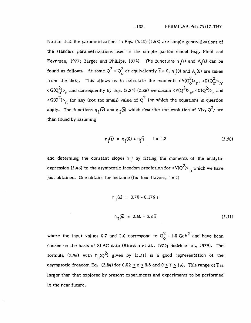
-108- FERMILAB-Pub-79 /17-THY
Notice that the parametrizations in Eqs. (5.46)-(5.48) are simple generalizations of
the standard parametrizations used in the simple parton model (e.g. Field and
Feynman, 1977; Barger and Phillips, 1974). The functions n im and Ai@ can be
found as follows. At some Q2 = Qz or equivalently ? = 0, ni(0) and Ai are taken
from the data. This allows us to calculate the moments < V(Qi)> n, <C (Qi)sn,
< G(Qz)>, and consequently by Eqs. (2.84)-(2.86) we obtain < V(Q2)>r,, <C (Q2) >n and
<G(Q2)>n for any (not too small) value of Q2 for which the equations in question
apply. The functions n ,(a and n 2@ which describe the evolution of V(x, Q2) are
then found by assuming
‘lie = rli(O) + rli's i= 1,2 (5.50)
and determing the constant slopes n il by fitting the moments of the analytic
expression (5.46) to the asymptotic freedom prediction for < V(Q2b n which we have
just obtained. One obtains for instance (for four flavors, f = 4)
q ,@ = 0.70 - 0.176:
q2(‘i) = 2.60 + 0.8s (5.51)
where the input values 0.7 and 2.6 correspond to Qz q 1.8 GeV2 and have been
chosen on the basis of SLAC data (Riordan et al., 1975; Bodek et al., 1979). The
formula (5.46) with qi(Q2) given by (5.51) is a good representation of the
asymptotic freedom Eq. (2.84) for 0.02 2 x 2 0.8 and 0 2 3 2 1.6. This range of S is
larger than that explored by present experiments and experiments to be performed
in the near future.
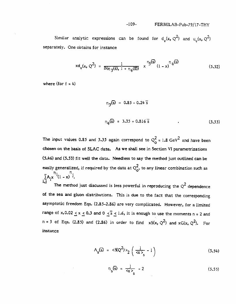
-lOP- FERMILAB-Pub-79/17-THY
Similar analytic expressions can be found for dv(x, Q2) and uv(x, Q2)
separately. One obtains for instance
x$,(x, Q2) = 1 B( n,(S), 1 + n4(9) (5.52)
where (for f = 4)
TJ,@ = 0.85 - 0.24;
n40 = 3.35 + 0.816s . (5.53)
The input values 0.85 and 3.35 again correspond to Qi = 1.8 GeV2 and have been
chosen on the basis of SLAC data. As we shall see in Section VI parametritations
(5.46) and (5.53) fit well the data. Needless to say the method just outlined can be
easily generalized, if required by the data at Qi, to any linear combination such as
lAixni(l - x)n j. i,i
The method just discussed is less powerful in reproducing the Q2 dependence
of the sea and gluon distributions. This is due to the fact that the corresponding
asymptotic freedom Eqs. (2.85-2.86) are very complicated. However, for a limited
range of x,0.02 < x c 0.3 and 0 es c 1.6, it is enough to use the moments n - - -- = 2 and
n = 3 of Eqs. (2.85) and (2.86) in order to find xS(x, Q2) and xG(x, Q2). For
instance
As@ = <s(Q2)> 2(&s-l) (5.54)
(5.5 5) Tl,o = -A- - 2 cx > S
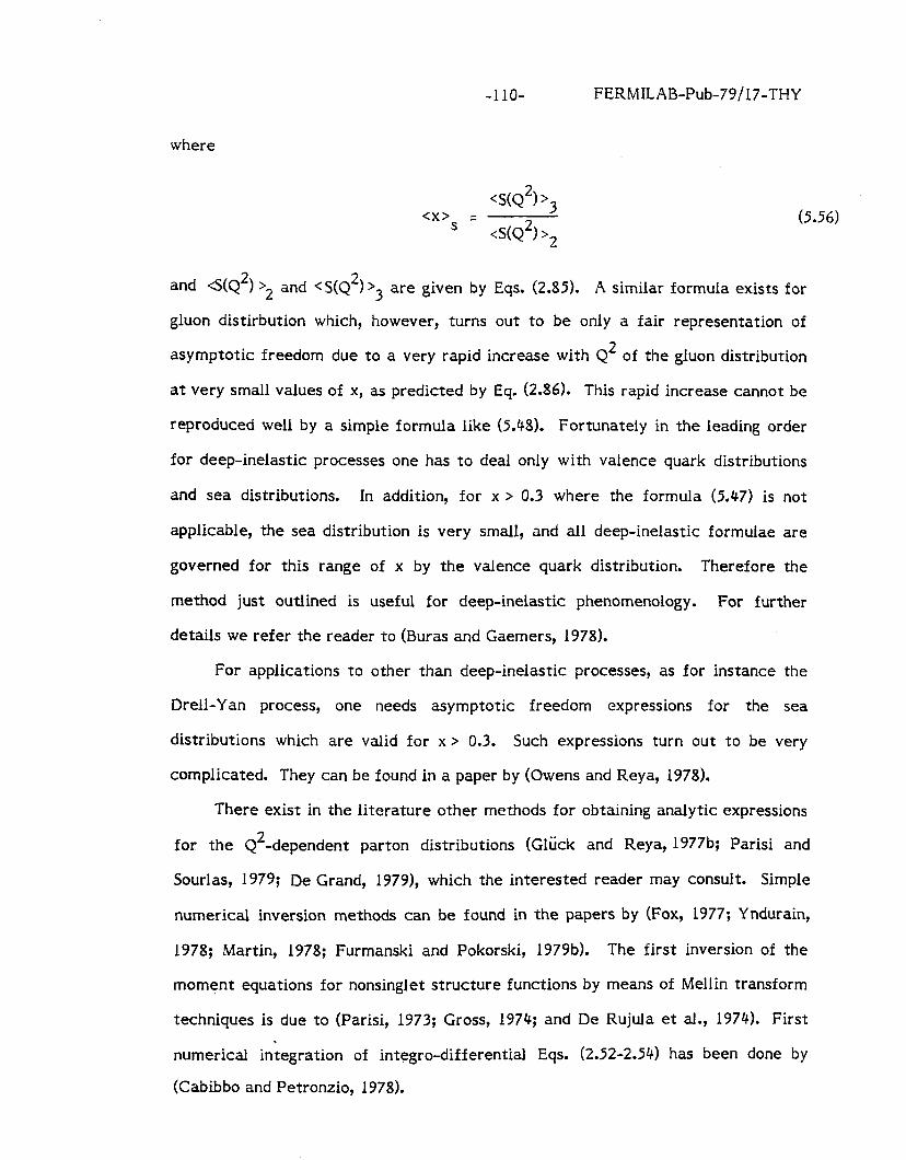
-llO-
where
<x> = <S(Q2) >3
S tStQ2) >2
FERMILAB-Pub-79/17-THY
(5.56)
and B(Q2) >2 and < S(Q2) > 3 are given by Eqs. (2.85). A similar formula exists for
gluon distirbution which, however, turns out to be only a fair representation of
asymptotic freedom due to a very rapid increase with QL of the gluon distribution
at very small values of x, as predicted by Eq. (2.86). This rapid increase cannot be
reproduced well by a simple formula like (5.48). Fortunately in the leading order
for deep-inelastic processes one has to deal only with valence quark distributions
and sea distributions. In addition, for x > 0.3 where the formula (5.47) is not
applicable, the sea distribution is very small, and all deep-inelastic formulae are
governed for this range of x by the valence quark distribution. Therefore the
method just outlined is useful for deep-inelastic phenomenology. For further
details we refer the reader to (Buras and Gaemers, 1978).
For applications to other than deep-inelastic processes, as for instance the
Drell-Y an process, one needs asymptotic freedom expressions for the sea
distributions which are valid for x > 0.3. Such expressions turn out to be very
complicated. They can be found in a paper by (Owens and Reya, 1978).
There exist in the literature other methods for obtaining analytic expressions
for the Q2-dependent parton distributions (Gliick and Reya, lP77b; Parisi and
Sourlas, 1979; De Grand, 1979), which the interested reader may consult. Simple
numerical inversion methods can be found in the papers by (Fox, 1977; Yndurain,
1978; Martin, 1978; Furmanski and Pokorski, 1979b). The first inversion of the
moment equations for nonsinglet structure functions by means of Mellin transform
techniques is due to (Parisi, 1973; Gross, 1974; and De Rujula et al., 1974). First
numerical integration of integro-differential Eqs. (2.52-2.54) has been done by
(Cabibbo and Petronzio, 1978).
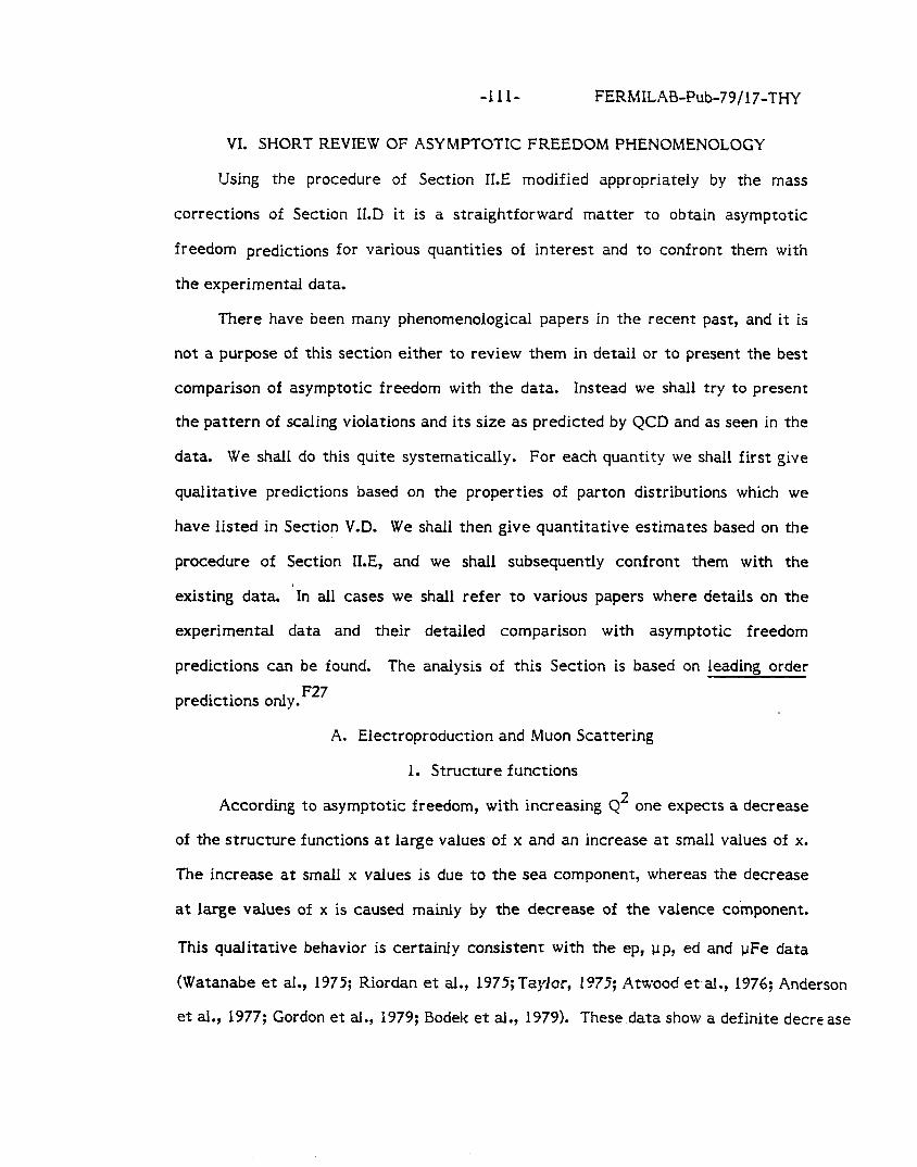
-lll- FERMILAB-Pub-79/17-THY
VI. SHORT REVIEW OF ASYMPTOTIC FREEDOM PHENOMENOLOGY
Using the procedure of Section 1I.E modified appropriately by the mass
corrections of Section 1I.D it is a straightforward matter to obtain asymptotic
freedom predictions for various quantities of interest and to confront them with
the experimental data.
There have been many phenomenological papers in the recent past, and it is
not a purpose of this section either to review them in detail or to present the best
comparison of asymptotic freedom with the data. Instead we shall try to present
the pattern of scaling violations and its size as predicted by QCD and as seen in the
data. We shall do this quite systematically. For each quantity we shall first give
qualitative predictions based on the properties of parton distributions which we
have listed in Section V.D. We shall then give quantitative estimates based on the
procedure of Section ILE, and we shall subsequently confront them with the
existing data. In all cases we shall refer to various papers where details on the
experimental data and their detailed comparison with asymptotic freedom
predictions can be found. The analysis of this Section is based on leading order
predictions only. F27
A. Electroproduction and Muon Scattering
1. Structure functions
According to asymptotic freedom, with increasing Q2 one expects a decrease
of the structure functions at large values of x and an increase at small values of x.
The increase at small x values is due to the sea component, whereas the decrease
at large values of x is caused mainly by the decrease of the valence component.
This qualitative behavior is certainly consistent with the ep, pp, ed and uFe data
(Watanabe et al., 1975; Riordan et al., 1975;Taylor, lY75; Atwood et-al., 1976; Anderson
et al., 1977; Gordon et al., 1979; Bodek et al., 1979). These data show a definite decrease
-112- FERMILAB-Pub-79 / 17-THY
of the structure function F2(x, Q2) for x > 0.25 and a Q2-independent behavior for
0.15 < x < 0.25. For x < 0.15 the data for ep and ed scattering are poor and nothing
definite can be said. The scaling violations in question increase with increasing x in
accordance with the increase of the anomalous dimensions with increasing n.
Asymptotic freedom fits, with or without mass effects, give good agreement with
the data above. The parameter A is found to be in the range 0.3 c A -C 0.5 GeV.
The details of such asymptotic freedom fits can be found in the papers by
(Parisi and Petronzio, 1976; De Rujula, Georgi and Politzer, 1977a; Cl&k and Reya,
1977a; Buras and Gaemers, 1978; Fox, 1977; Tung, 1978; Kogut and Shigimitsu,
1977a; Johnson and Tung, 1977a, b). We show a typical asymptotic freedom fit in
Fig. 12. The best data for structure functions at small values of x come from pp
scattering (Anderson et al., 1977; Gordan et al., 1979). F28 For x < 0.15, and
especially for x < 0.10, a definite increase with Q2 of FgP is observed. As shown in
Fig. 13, the agreement of asymptotic freedom with the data is again good with a
value of A consistent with that obtained from ep and ed scattering. We should like
to remark that the increase at small values of x is expected to be caused by the
increase of both the non-charmed sea as well as of the charmed sea component of
the proton.
The data above extend over the range of Q2 up to 60 GeV2 with the majority
of experimental points below Q2 = 30 GeV2. Recently results from a u Fe
experiment have been reported for Q2 up to 150 GeV (Ball et al., 1979). The
scaling violations observed in this experiment agree well with asymptotic freedom
predictions for Q2 < 20 GeV2 but disagree with it for larger values of Q2. In fact a
decrease of the structure functions for 0.15 < x < 0.25 and for Q2 < 20 GeV2 is
followed by an increase for Q2 > 20 GeV2. Whether these data cause a problem for
-113- FERMILAB-Pub-79/17-THY
QCD remains to be seen. The effect is much too strong to be explained by new
flavor production with the conventional charge assignment. It is of great interest
to see whether the new u-experiments at CERN and at Fermilab will confirm the
finidng of Ball et al.
2. Moment analysis
Anderson, Matis and Myrianthopoulos (1978) have made a comparison of the
asymptotic freedom predictions for the moments of F2(x, Q2) with the experimen-
tally extracted Nachtmann moments as defined by Eq. (2,124). Their analysis
includes ep, ed and up data. The agreement of QCD with the data is impressive as
can be seen in Fig. 14. The preferred value of the parameter A turns out to be
0.66 +, 0.08 GeV, a slightly higher value than that obtained from the direct analysis
of the structure functions.
B. v and7 Deep Inelastic Scattering (Charged Current)
Asymptotic freedom predictions for v and v deep-inelastic scattering can be
obtained by means of the parton model formulae of Section II and the Q2 dependent
parton distributions of Section V.
1. Total cross-sections 3 In the simple parton model the total cross-sections ov /Ev and CJ /EC are
independent of energy except for possible threshold effects due to heavy quark u v production. In addition o /o = v v l/3 in the absence of sea quarks and o /o :: 0.40
if the sea carries 5%-10% of the momentum of the nucleon as observed at
Gargamelle (E :: 5 GeV) (Eichten et al., 1973; Deden et al., 1975). In the presence
of asymptotic freedom effects o v’ 5 u v and also o /b depend on energy. This
energy dependence arises as follows. With increasing energy, a larger range of Q2
is explored and, consequently, the valence and sea contributions to any of the
cross-sections are effectively decreased and increased, respectively. The sea
contribution to v and T cross-sections is roughly the same except for the difference
-114- FERMILAB-Pub-79/17-THY
in charm production. On the other hand, the valence quark contribution is roughly 3
times larger in the v cross-section. Consequently in the range of energies explored
by present experiments, the energy dependence of (3” is expected to be governed by
the decrease of the valence quark distribution, i.e., ov /E is expected to fall
(Hinchliffe and Llewellyn-Smith, 1977b) with increasing energy. For v scattering
the decrease of the valence quark contribution is roughly compensated by the
increase of the sea. Thus “J/E is expected to be roughly constant at moderate
energies. At higher energies, where charm production is at full strength, a~ /E is
expected to rise slowly. Asymptotically it should approach ov /E. In summary, in
the range of energies explored by present experiments, one expects a decrease of
o” /E and a constant behavior followed by an increase for “3/E. Consequently the
ratio ~;/cr~ is expected to increase. These expectations (Al tarelli, Petronzio and
Parisi, 1976; Barnett, Georgi and Politzer, 1976; Buras, 1977; Glijck and Reya,
1977a; Barnett and Martin, 1977; Hinchliffe and Llewellyn-Smith, 197733; Buras and
Gaemers, 1978; Barger and Phillips, 1978; Fox, 1978; Avilez et al., 1977; Graham et
al., 1977; Roy et al., 1977) are confirmed by the recent high energy experiments
BEBC (Bosseti et al., 19771, CALT (Barish et al., 1977b; 19781, Serpukhov
(Asratyan, 1978) and CDHS (de Groot et al., 1979a) when combined with low energy
data as is shown in Figs. 15 and 16. We should like to remark, however, that above
E = 40 GeV the changes in the cross-sections are very weak both in the theory and
experiment, and to a good approximation the total cross-sections in the range
40 < E < 200 GeV can be represented by a simple parton model formula with Q2-
independent quark distributions, with the amount of the sea (valence) larger
(smaller) than that observed at Gargamelle.
The very slow change of the total cross-sections with energy is easily
understood. Integrating over x amounts to summing up the increasing and
decreasing with Q2 parts of the structure functions which compensate partly each
-115- FERMILAB-Pub-79/17-THY
other leading to a small ef feet. The same phenomenon happens in the case of c y >
on which we now comment briefly.
2. <y’
In the simple parton model for the strong interactions and for the structure of
weak interactions given by the Weinberg-Saiam model the distributions 1 duv
1 d% E dy and
E 7 are, in the absence of the sea quarks in the nucleon, flat and fl (1 - Y)~,
respectively. Consequently <yS = 0.5 and <y >y = 0.25. If the sea carries 5%-10%
momentum of the nucleon as observed at Gargamelle the distributions 1Q
1 d?J E -$ and
-- E dy
have additional small (1 - y)2 and small flat components respectively which
lead to <y >L, = 0.48 and <y >; = 0.3. If strong interactions as described by QCD are
switched on, the sea component increases and the valence component decreases
with energy. Consequently <y $ and <yT are expected to decrease and increase
with energy, respectively. These expectations are confirmed by the recent high en-
ergy experiments, CITFR (Barish et al., 1977a. 1978) and CDHS (De Groot, 1979a)
as shown in Fig. 17. The rate of change is, as in the case of total cross-sections,
very slow. In particular the CDHS group hardly sees any dependence. At
E = 200 GeV (Y ’ v " 0.46 and <y>i z 0.34. Asymptotically we expect
<Y’ V = ‘y>T = 0.44. Therefore if nothing but asymptotic freedom effects are
present at higher energies one should observe a detectable increase of ‘~‘3, but
almost constant <y> . 1 day
These slow changes with energy of < Y>~ and <Y>~, as well
lVd% -- as Of E dy and E dy - -, predicted by asymptotic freedom are very fortunate
because they will not mask the changes in y distributions due to W boson
propagator. The latter effect (for mW = 80 GeV) is much stronger in the range
500 < E c lo4 GeV than asymptotic freedom effects. We refer the interested
reader to a paper by Halprin (1978JF2’ where a detailed study of the W boson
propagator effects in y distributions can be found.
3. <x>, <xy>, cx” >
More useful quantities to test asymptotic freedom ideas than those discussed
in B-1 and 8.2 are the averages <x > and <xy>, or, more generally, the moments
-116- FERMILAB-Pub-79/17-THY
<x”> = ; J dx x” g , (6.1)
<xmyn> = is.r mn da
dx dy x Y dxay . (6.2)
On the basis of the properties of the Q2 dependence of parton distributions listed in
Section V.D and the formulae of Section II.B, both c x” > and <xmyn > should
decrease with increasing energy. As an example we show in Fig. 18 the data for
<Q2/E > = 2M<xy > which exhibit the expected energy dependence. The solid curve
in the figure corresponds to a typical asymptotic freedom fit with n = 0.5 GeV.
The data are from GGM (Eichten et al., 1973), BEBC (Bosetti et al., 1977), FNAL
(Berge et al., 1976), SKAT (Baranov et al., 1978) and CDHS (De Groot et al., 1979a)
and IHEP-ITEP (Asratyan et al., 1978).
4. ./ dx Fi(x, E) and I dx xnFi(x, Eh)
If asymptotic freedom or any renormalizable field theory ideas are correct,
then the structure functions Fi do not depend directly on the incoming energy E but
on Q2. This is obvious if we recall the intuitive picture of Section V.A. Therefore
it is not a very convenient way to test asymptotic freedom ideas by measuring the
integrals J’ dxFi(x, E). Experimentally they are extracted by using simple parton
model formulae and assuming factorization in x and y. This last assumption is not
true in QCD. The only way to compare the integrals of the structure functions in
question as presented for instance in the papers by (Bosetti et al., 1977; Barish et
al., 1978) is to relate them to the total cross-sections
latter using asymptotic freedom formulae as discussed
is made in Fig. 19 where we have used the relations
ov and -v and calculate the
previously. Such an exercise
+% 1,l F2(x, E)dx = 3TF ov E 4G2M
(6.3)
-i I?- FERMILAB-Pub-79/17-THY
Jo:F3(x, E)dx = + o’; O3 2G M
. (6.4)
The integral in Eq. (6.3) measures essentially the fraction of the proton
momentum carried by quarks and antiquarks. This fraction decreases very slowly
since some of the momentum is effectively transferred to gluons. The decrease of
the integral in Eq. (6.4) is mainly due to the decrease of the valence component of
the nucleon. Asymptotically the integral of F3 is expected to be zero.
.vnore sensitive tests of asymptotic freedom can be made by measuring the
moments
1 s dx X”Fi(X, Eh)
0 (6.5)
where Eh is the hadronic energy which is related to Q2 by
Q2 = 2xv = 2xM(Eh - M) = 2xMEh . (6.6)
In order to calculate the Eh dependence of the moments in Eq. (6.5) in the
framework of asymptotic freedom one computes first Fi(x, I$ from Fi(x, Q2) by
using Eq. (6.6). Subsequently the moments of Eq. (6.5) are calculated by a
straightforward integration. It should be however kept in mind that for finite fixed
energy Eh the lower limit of integration corresponds to Q2 = 0 for which
perturbative calculations do not make sense. If we take QZmin = 2 GeV2 to be the
minimal value of Q2 for which perturbative calculations are reliable then for
Eh = 5 GeV, 20 GeV and 200 GeV the corresponding minimal values of x are 0.10,
0.025 and 0.0025. Therefore only for $1 > 20 GeV can we reliably estimate the
n = 0 moment of Eq. (6.5) in perturbation theory. The situation is better for n > 0
-118- FERMILAB-Pub-79/17-THY
because these moments receive only a very small contribution from very small x
regions. In Fig. 20, which we took from the paper by (de Groot et al., 1979a), we
show the average values
x - .f ’ x F2(x, E,)dx/.f F2- 0
’ F 0 2
(x, Eh)dX
and
:F =I 1 2 3 0
x F3(x, Eh)dx/ j- ’ xF3k, JQdx 0
(6.7)
(6.8)
as functions of 5-I . The solid curve is the asymptotic freedom prediction with
A = 0.47 GeV.
5. x distributions
From the properties of parton distributions as discussed in Section V.D and 1 1 do. the formulae of Section 1I.B it immediately follows that the distribution E 17 dx in
both v and T processes should increase and decrease with energy at small and large
x values, respectively. These trends are in agreement with the existing high energy
data. We refer the interested reader to the paper by (Fox, 1978 ) where a detailed
comparison of asymptotic freedom predictions with the experimentally measured x
distributions has been made. Also very recent data for x distributions (Benvenuti et
al., 1979) exhibit the expected pattern of scaling violations. The x distributions
deserve certainly further experimental studies since among the quantities which
directly depend on energy and not on Q2 the quantities in question are expected to
show the largest asymptotic freedom effects.
-i 1% FERMILAB-Pub-79/17-THY
6. v and-3 structure functions
So far we have discussed only the energy dependence of various quantities
which can be measured in v and 3 induced processes. We concluded that, except
for the x distributions and the moments (6.51, the measurements of the energy
dependence are not very sensitive tests of asymptotic freedom ideas. Certainly the
best way to compare the theory with the data is to consider the structure functions
as functions of Q2. The Q2 dependence of FzyV is expected to be similar to that of
Fep i e 2’ l * they should increase at small values of x and decrease at large values of
x. On the other hand, the Q* dependence of F3 should be similar to that of the
valence quark distribution. These expectations are confirmed by the recent high
energy data obtained at CERN (Bosseti et al., 1978; de Groot et al., 1979a, b). As
an example we show in Fig. 21 the Q2 dependence of Fz as measured by de Groot
et al. The solid lines correspond to an asymptotic freedom fit with A = 0.47 GeV.
7. Moment analyses of BEBC and CDHS
One of the predictions of QCD is the n dependence for the anomalous
dimensions of various operators. This n dependence can be tested indirectly by
comparing the scaling violations as predicted by the theory with the experimental
data. Such a test is not ideal because one has to make assumptions about the
structure functions or parton distributions (in particular about the gluon distribu-
tion) at some value of Q2 = Q’, and for the whole range of x. Also there is one free
parameter, A. It would be useful to have a direct way of experimentally
“measuring” the n dependence of the anomalous dimensions in experiment. This is,
in fact, possible for the non-singlet anomalous dimensions as has been suggested
and measured by the BEBC group (Bosseti et al., 1978). Recently a similar analysis
has also been carried out by the CDHS group (de Groot et al., 1979c). Consider the
moments of the structure function F3 which in QCD are given as follows
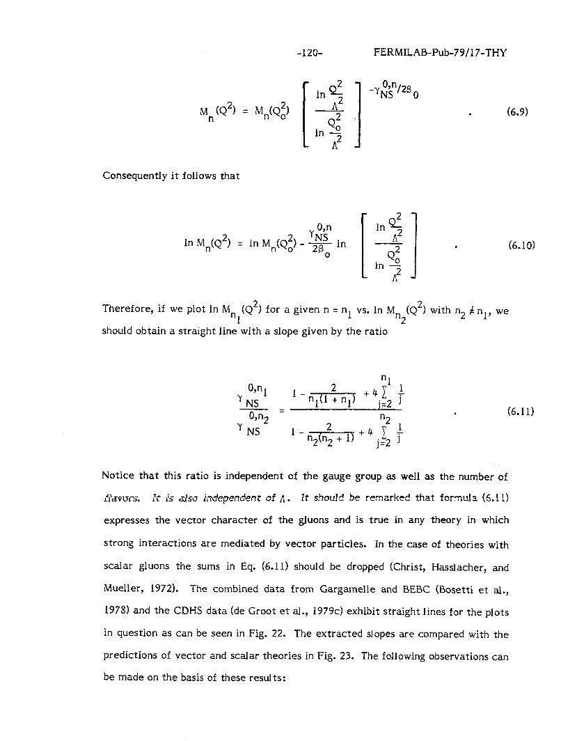
-120- FERMILAB-Pub-79/17-THY
Mn(Q2) = M&Q;)
Consequently it follows that
Q‘ In 0
- A2
O,n yNS In Mn(Q2) = In Mn(Qz) - 28 In
0
. (6.9)
. (6.10)
Therefore, if we plot In M “1
(Q2) for a given n = n1 vs. In M “2
(Q2) with n2 f nl, we
should obtain a straight line with a slope given by the ratio
OJY 1 2 “1
’ NS - nl(l+“l) +4l c
.=2 J 0,n2 = . (6.11)
’ n2
NS 2 ‘-iii +4 7 1 5- jC2 1
Notice that this ratio is independent of the gauge group as well as the number of
iYaolxs. f; Is &u indepedem of A. It should be remarked that formula (5.11)
expresses the vector character of the gluons and is true in any theory in which
strong interactions are mediated by vector particles. In the case of theories with
scalar gluons the sums in Eq. (6.11) should be dropped (Christ, Hasslacher, and
Mueller, 1972). The combined data from Gargamelle and BEBC (Bosetti et al.,
1978) and the CDHS data (de Groot et al., 1979c) exhibit straight lines for the plots
in question as can be seen in Fig. 22. The extracted slopes are compared with the
predictions of vector and scalar theories in Fig. 23. The following observations can
be made on the basis of these results:
-121- FERMILAB-Pub-79/17-THY
i) Gargamelle-BEBC results agree very well with the formula (6.11) and
disagree with the predictions of the scalar theory (Ellis, 1978).
ii) The ratios of the ordinary moments (Cornwall and Norton, 1969) extracted
by the CDHS group favor the vector theory whereas the ratios for the Nachtmann
moments lie al most exactly between predictions of vector and scalar gluon
theories.
iii) The predictions of the scalar theory are systematically below all the data
We may therefore conclude that the results above give some support to the belief
that the mediators of strong interactions are spin-l particles. Recently Abbott and
Barnett (1979)F31 reanalyzed the data of BEBC and CDHS and investigated how the
plots in Figs. 22 and 23 depend on the cuts in Q2 and how they could be effected
by higher-twist contributions. Their analysis weakened somewhat the conclusion made
above. We refer the reader to this interesting paper for details.
It should be remarked that although the plots of Figs. 22 and 23 may help to
distinguish between vector and scalar theories, only ratios of anomalous dimensions
are “measured” in this way. By taking ratios, some of the predictions of the theory,
namely the size of the anomalous dimensions, are lost. Furthermore, the anomalous
dimensions of non-singlet operators which we discussed here represent only a part
of the theory in which singlet operators are also present. Therefore to test the
theory more critically and in particular to distinguish it from other vector theories,
it is necessary to study the full QL evolution of structure functions with both
singlet and non-singlet contributions taken into account, as we did in the previous
subsections. Discussion of the predictions of other field theories will be presented
below.
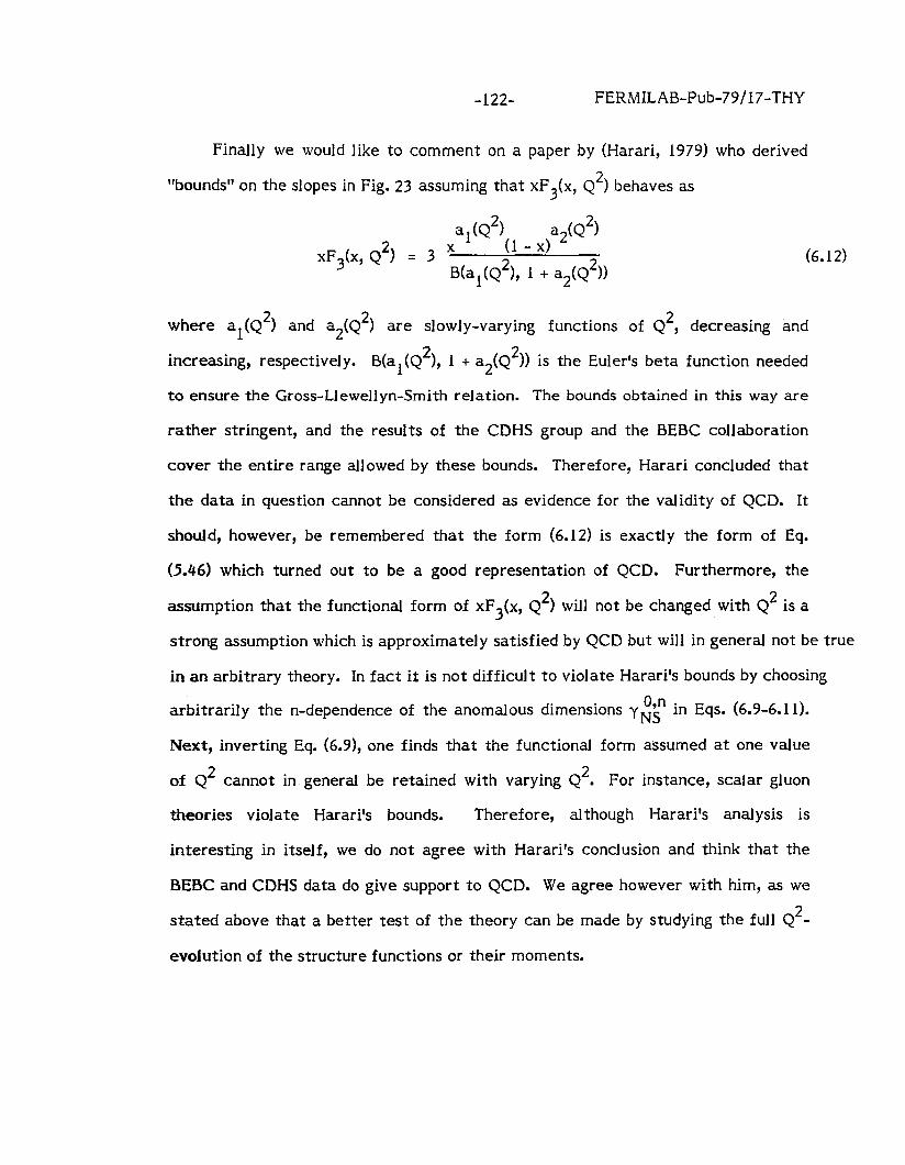
-122- FERMILAB-Pub-79/17-THY
Finally we would like to comment on a paper by (Harari, 1979) who derived
“bounds” on the slopes in Fig. 23 assuming that xF3(x, Q2) behaves as
xF3(x, Q2) = 3 ’ al(Q2)
(1 -x) a2(Q2)
B(al(Q2), 1 + a2(Q2)) (6.12)
where aI and a2(Q2) are slowly-varying functions of Q2, decreasing and
increasing, respectively. B(al(Q2), 1 + a2(Q2)) is the Euler’s beta function needed
to ensure the Gross-Llewellyn-Smith relation. The bounds obtained in this way are
rather stringent, and the results of the CDHS group and the BEBC collaboration
cover the entire range allowed by these bounds. Therefore, Harari concluded that
the data in question cannot be considered as evidence for the validity of QCD. It
should, however, be remembered that the form (6.12) is exactly the form of Eq.
(5.46) which turned out to be a good representation of QCD. Furthermore, the
assumption that the functional form of xF3(x, Q2) will not be changed with Q2 is a
strong assumption which is approximately satisfied by QCD but will in general not be true
in an arbitrary theory. In fact it is not difficult to violate Harari’s bounds by choosing
arbitrarily the n-dependence of the anomalous dimensions yNs Oyn in Eqs. (6.9-6.11).
Next, inverting Eq. (6.91, one finds that the functional form assumed at one value
of Q2 cannot in. general be retained with varying Q2. For instance, scalar gluon
theories violate Harari’s bounds. Therefore, al though Harari’s analysis is
interesting in itself, we do not agree with Harari’s conclusion and think that the
BEBC and CDHS data do give support to QCD. We agree however with him, as we
stated above that a better test of the theory can be made by studying the full Q2-
evolution of the structure functions or their moments.
-123- FERMILAB-Pub-79/17-THY
8. Comments on neutral current processes
In QCD, scaling violations are also expected in the neutral current processes
(Barnett and Martin, 1977; Buras and Gaemers, 1977; Barger and Phillips, 1978;
Hinchliffe and Llewellyn-Smith, 1977c). In particular, the well-known plot Rv vs. R;
is expected to change with energy. The present data on neutral currents are, however,
not precise enough to make any QCD analysis meaningful.
C. Comments on Fixed Point Theories
Until now our discussion of scaling violations concentrated on asymptotically
free gauge theories. Here we shall comment on theories in which the effective
coupling constant approaches for Q 2-+ QJ a constant value g* f 0 (so-called fixed
point at which B(g*) = 0). If g* is small then we may hope to calculate predictions
of these theories in perturbation theory in g*. It should be emphasized however
that the structure of fixed point theories is not well known. In particular, we do
not know whether a fixed point with a small value of g* exists. Therefore if we
assume g* to be small, use perturbation theory and show that the result disagrees
with the data, we still cannot claim that we have ruled out the theory in question.
It could namely happen that g* was large in fact and the true prediction of the
theory obtained by non-perturbative methods was consistent with the data.
Nevertheless it is interesting to see what happens if perturbation theory is
used. Since the ratios of anomalous dimensions in scalar gluon theories (obtained in
perturbation theory) are systematically below BEBC and CDHS data, we shall
discuss here only abelian vector theories. These theories have been studied
extensively by (Gliick and Reya, 1976, 1977a, 1979) and we shall only recall the
most important points of their analysis.
For the moments of non-singlet structure functions we have
-124- FERMILAB-Pub-79/17-THY
2 MNS(n Y Q2) = MNS(n Q*)exp - s ‘In Q ’ 0 c)
= M%, Q;) -I;iL’
where rlin is determined by its fixed point value
y;;” = ‘4E L 3 + ag
*4
j=2 1 1 .
(6.13)
(6.14)
The n dependence of yzs is exactly the same as in QCD. The Q2 dependence
in Eq. (6.13) is different but as noticed first by (Tung, 1975; Llewellyn-Smith, 1975) if g* is
properly chosen Eq. (6.13) can mimic the corresponding QCD prediction in the
range of Q2 available in present experiments. In particular Reya (1979) and Abbott and
Barnett (1979) find that abelian vector theories agree well with CDHS and BEBC data for
the moments of F3 if g *2
/161~~ z 0.04. Therefore if g* is small and the leading order formu-
lae (6.13)-(6.14) are used, the fixed point vector gluon theories cannot be at present
distinguished from QCD on the basis of scaling violations observed in non-singlet
structure functions. It has been pointed out however by Gliick and Reya that such a
distinction can be made on the basis of the singlet structure functions. They
propose to look at the second moment of FzN(x, Q2), which in the parton language
measures the fraction of the proton momentum carried by the quarks. In
experiment the moment in question is roughly equal to 0.5 at low values of Q2 and
decreases very slowly with increasing Q2. It turns out that only QCD and so-called
“fixed point QCD” (FP-QCD, QCD with the vanishing triple gluon vertex) agree
with this behavior. All other theories considered by Gliick and Reya predict an
increase of the second moment with Q2 (as pointed out by Abbott and Barnett (1979))
higher twist effects could invalidate these results).
-12% FERMILAB-Pub-79/17-THY
Gliick and Reya (1979) investigated also the full x and Q* dependence of
F\:N(x, Q*) and concluded that further discrimination between QCD and the FP-
QCD cannot be made on the basis of the present data on scaling violations.
Once again we would like to emphasize that when judging these results one
should keep in mind that the predictions of fixed point theories as discussed here
cannot be treated on the same footing as the QCD predictions. The reason is that
whereas we can believe in the results of perturbative calculations in QCD, there is
no reason that such calculations are justified for fixed point theories.
D. Critical Summary
As we have seen in this Section, asymptotic freedom (leading order)
predictions agree well with the scaling violations observed in ep, ed, up, v N and TN
deep-inelastic scattering. We should, however, be very careful in judging these
results. The reasons are as follows:
a) The mass corrections, which enter any asymptotic freedom analysis, are,
on the one hand, non-negligible at low values of Q* and, on the other hand, as
discussed in Section II not completely understood. Presumably the problem of
target mass corrections cannot be completely solved within perturbation theory.
The effects of heavy quarks can however be discussed in the framework of
perturbation theory except for the region close to various thresholds, where non-
perturbative effects are probably important. Since the ultimate QCD predictions
depend on the treatment of mass and threshold effects, further study of the effects
in question is very desirable. One way to circumvent partially the problem of mass
correction is to make QCD comparison with the data for (4x2m2/Q2) << 1, where
at least target mass effects are expected to be small.
-126- FERMILAB-Pub-79/17-THY
b) The effects of higher twist operators, which we have not included in our
analysis, may turn out to be of some importance at low values of Q*:: 0 (5 GeV2)
(for a recent analysis see Abbott and Barnett, 1979).
c) There is the question whether the use of leading order predictions at low
values of QL is justified in view of the existence of calculable higher order
corrections. We shall try to answer this question in the next two Sections.
-127- FERMILAB-Pub-79/17-THY
VII. HIGHER ORDER ASYMPTOTIC FREEDOM CORRECTIONS TO DEEP-INELASTIC SCATTERING (NON-SINGLET CASE)
A. Preliminaries
In the last three sections we have discussed leading order predictions of
asymptotic freedom for deep-inelastic processes. We have seen that these
predictions are in a good agreement with all experimental data with the value of
the scale parameter fl in the range from 0.3 GeV to 0.7 GeV. However, at
Q2 z few GeV* the leading asymptotic behavior cannot be the whole story and it is
of interest and of importance to ask whether higher order corrections in the
effective coupling constant g2(Q2) modify these results. In this and the next
section we shall discuss these corrections in great detail. We shall see that these
corrections are different for different structure functions and consequently various
parton model relations and current algebra sum rules, which were true in the
leading order, are no longer satisfied. The experimental verification of the
violations of these sum rules is very important although a difficult task.
There is still another reason why higher order calculations are important.
This is the fact that without them the value of A cannot be extracted from
experiment in a theoretically meaningful way (Bate, 1978). To see this consider
the moments of a non-singlet structure function as given by the leading order
expression and, to simplify the argument, take the appropriate roots
*@O -O,n
hn(Q2) 5 [ M,(Q*) 1 Y’s = ~,ln-$- . flLO
(7.1)
where An are Q*-independent numbers. If the experimentally measured moments
are
-12%
42 An In 0.49
FERMILAB-Pub-79/17-THY
(7.2)
then (in units of GeV)
A LO = 0.7
Now let us introduce next to the leading order corrections to the leading order
formula (7.1) and write it as
+Q*) = A,ln g +R A2n l (7.3)
If Rn = 6 An, where 8 is an n independent number, then we can rewrite (7.3) as
Gn(Q2) = An In Q ,:
with
Iv2 = A2em6
(7.4)
Now we have various options. We can work with Eq. (7.4) and say that we have
absorbed all higher order corrections by redefining the parameter A. In that case
A’ = ALO. We can also work with expression (7.3) but in this case
(7.5)
A2 = e6A2 LO (7.6)
-129- FERMILAB-Pub-79/17-THY
In practice Rn is not proportional to $, but one can always redefine A (Bardeen,
Buras, Duke, Muta, 1978) by using the equality
inIn $+R 2
A* n = AnlnQ
A2 I + [R,-&A,1 (7.7)
The freedom in defining A, as discussed here, is related to the freedom which we
have in defining the effective coupling constant g*(Q*) when solving renormali-
zation group equations. (F or more details, see Section VI1.F.) All these examples
show clearly that one cannot discuss numerical values of A in a theoretically
meaningful way without calculating higher order corrections and without specifying
the definition of the effective coupling constant.
Once a definition of g*(Q*) is made and is used in calculations of higher order
corrections in various processes it is possible to make a meaningful comparison of
higher order corrections to various processes. We shall see that these corrections
are generally different for different processes. This teaches us that it is in
principle unjustified to use the same value of A in the leading order expressions for
different processes. On the other hand, once higher order corrections are included
in the analysis and g2(Q2) is properly defined in a universal way, it is justified to
use the same value of A in different processes. We shall discuss all these questions
in greater detail and with specific examples, but first we have to calculate the
higer order corrections. As we shall see there are many subtle points related to
higher order calculations which one does not encounter in the leading order. These
are, for instance, various gauge dependences and renormalization prescription
dependences of separate elements of the higher order formulae. We shall deal with
all these questions in detail.
-130- FERMILAB-Pub-79117-THY
B. Wilson Coefficient Functions of Non-singlet Operators to Order g*
We begin the discussion of higher order corrections with the non-singlet
structure functions (e.g. F2 ep - F;“, F:p - FzP, F3, etc.) which we generally denote
by FfiJ’(x, Q*). In Quantum Chromodynamics the moments of FFS(x, Q*) are given
as follows
1 k = L,* (7.8)
. (7.9)
Here C~sn(Qzh* , g*> are the Wilson coefficient functions of the non-singlet
operators and An NS(U2) are the corresponding reduced hadronic matrix elements.
The ANSI s n are uncalculable by present methods and as discussed in the previous
sections must be taken from experiment. The coefficient functions
C;sn(Qz/ u*, g*) are, on the other hand, calculable in perturbation theory. They
satisfy the renormalization group equations (4.8) which have the following solution
= Cisn(l, g*)exp $Q*) Y;&‘)
&.I *I dg’ TpT 1 (7.10)
where Y is(g) is the anomalous dimension of the non-singlet operator O\s and -2 2 g (Q ) is the effective coupling constant. i*(Q*) satisfies the equation
& - g@@ ; gtt = O) = g . (7.11)
-131- FERMILAB-Pub-79/17-THY
Here t = In Q*/u * and g is the renormalized strong interaction coupling constant.
In order to find explicit expressions for the leading and next-to-the-leading
contributions to Cr;fFn(Q2/p2, g*) we expand y is@, B @ and Ctsn(l, i*) in powers
k&n ii* (l),n &@ = yNS 16-2 + ‘NS ? (7.12)
? (7.13)
and (through order g*)
c;rn(l, i*, =
k = 2,3
k=L
. (7.14)
k Here 6NS are constants which depend on weak and electromagnetic charges.
Inserting Eqs. (7.12)-(7.14) into Eq. (7.10)) expanding in i*(Q*) and inserting
the result into Eqs. (7.8) and (7.9)) we obtain after putting u* = Q:
d”
f$%, Q*) = 6ks A:+Q:) 1 + I g*(Q*) - ji*(Q;, 1
161~’ RNS
R2tQ21 NS
k,n I[ 3 g*(Q;)
k = 2,3
where (7.15)
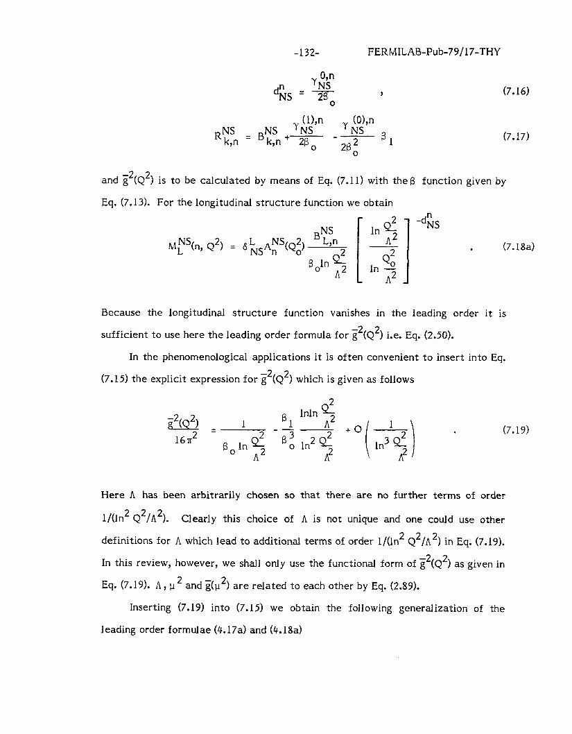
-132- FERMILAB-Pub-79/17-THY
0 ‘NS
d”Ns = 28 ? 0
RNS NS k,n = Bk,n+
and g*(Q*) is to be calculated by means of Eq. (7.11) with the P function given by
Eq. (7.13). For the longitudinal structure function we obtain
(7.16)
(7.17)
hlNS(n Q*) = 6 L L ’ NsA;s(Q;) lnd
A*
Q2 In 0
A* 1 -dFlS . (7.18a)
Because the longitudinal structure function vanishes in the leading order it is
sufficient to use here the leading order formula for g*(Q*) i.e. Eq. (2.50).
In the phenomenological applications it is often convenient to insert into Eq.
(7.15) the explicit expression for g*(Q*) which is given as follows
1 Bl -- f33
0
lnln Q A’
ln2 2 A*
+o 1
ln3 2 8
. (7.19)
Here h has been arbitrarily chosen so that there are no further terms of order
l/(ln* 4*/h*). Clearly this choice of A is not unique and one could use other
definitions for h which lead to additional terms of order l/(ln* Q*/h*) in Eq. (7.19).
In this review, however, we shall only use the functional form of g*(Q*) as given in
Eq. (7.19). A, 1-1~ and $u*) are related to each other by Eq. (2.89).
Inserting (7.19) into (7.15) we obtain the following generalization of the
leading order formulae (4.17a) and (4.18a)
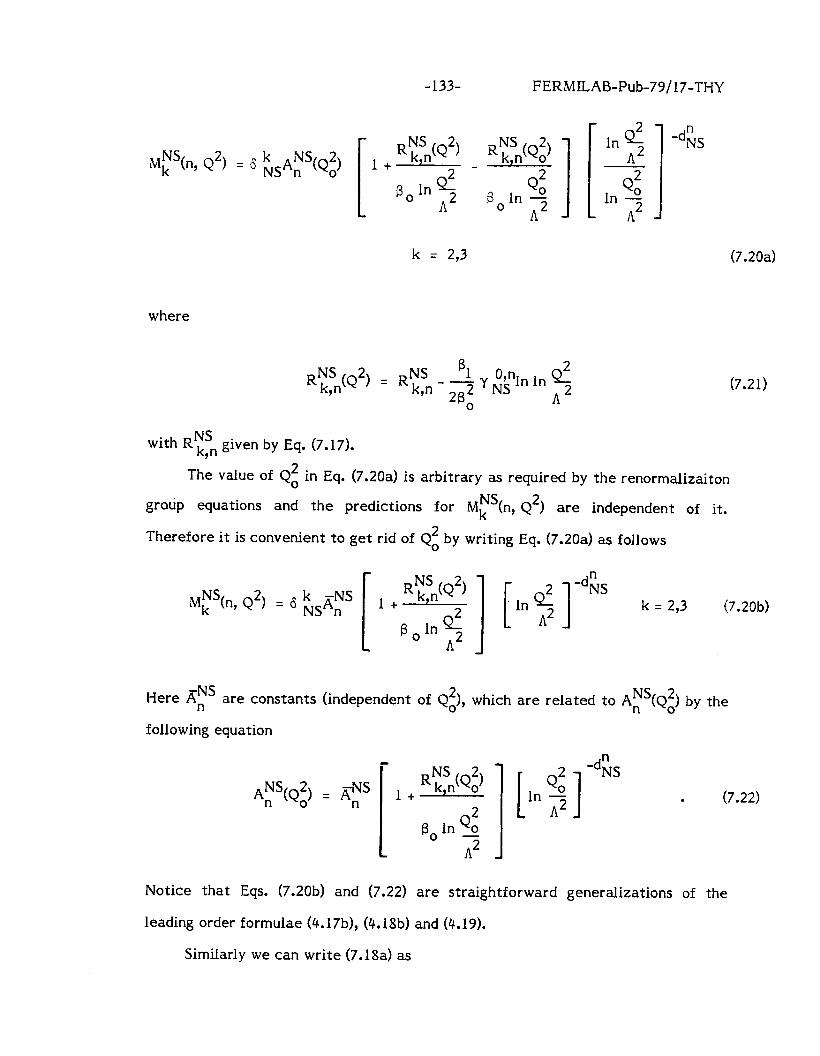
-133- FERMILAB-Pub-79/17-THY
MNS(n Q*) = 6 k NS * k ’ NSAn (Qo)
k = 2,3
where
5 R;yn(Q2) = R;sn - - y Oynln In Qz 28* NS
0 A*
lnd A* [ 1 Q2
In o A*
-dk5
(7.20a)
with RFSn given by Eq. (7.17). ?
The value of QE in Eq. (7.20a) is arbitrary as required by the renormalizaiton
group equations and the predictions for MfiJ’(n, Q*) are independent of it.
(7.21)
Therefore it is convenient to get rid of Qi by writing Eq. (7.20a) as follows
i 1 ‘lnQ f
-dl& k = 2,3 (7.20b)
Here A:’ are constants (independent of Qz), which are related to Ar’(Qz) by the
following equation
ANS(Q2) = KNs n 0 n I l + R~S,(Q~)
2 B, In Q,
A*
. (7.22)
Notice that Eqs. (7.20b) and (7.22) are straightforward generalizations of the
leading order formulae (4.17b), (4.18b) and (4.19).
Similarly we can write (7.18a) as
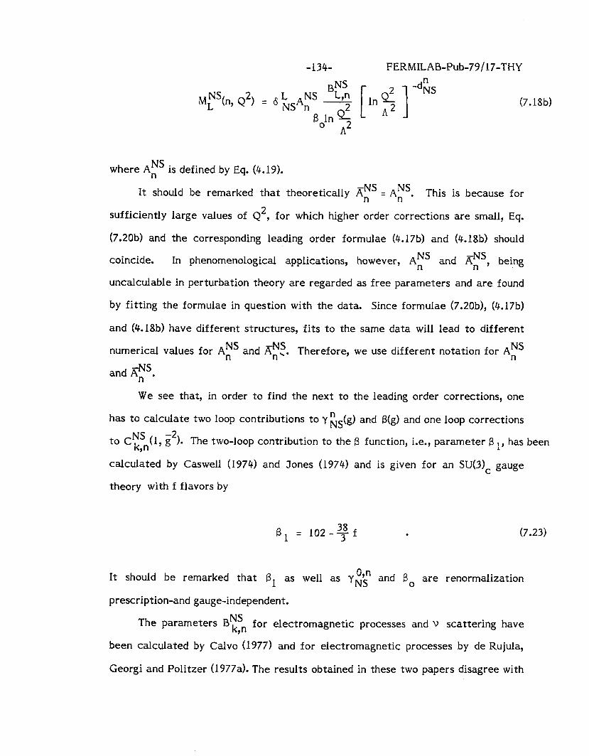
-134- FERMILAB-Pub-79 /17-THY
MN% Q*) = 6 L ’ (7.18b)
where A:’ is defined by Eq. (4.19).
It should be remarked that theoretically A:’ q A:‘. This is because for
sufficiently large values of Q*, for which higher order corrections are small, Eq.
(7.20b) and the corresponding leading order formulae (4.17b) and (4.18b) should
coincide. In phenomenological applications, however, n ANS and AZ’, being
uncalculable in perturbation theory are regarded as free parameters and are found
by fitting the formulae in question with the data. Since formulae (7.20b), (4.17b)
and (4.18b) have different structures, fits to the same data will lead to different
NS numerical values for An and $I:. Therefore, we use different notation for AfS
and A:‘.
We see that, in order to find the next to the leading order corrections, one
has to calculate two loop contributions to y n NS(g) and 8(g) and one loop corrections
to CFsn(l, g*,. Th e t ’
wo-loop contribution to the 8 function, i.e., parameter 8 1, has been
calculated by Caswell (1974) and Jones (1974) and is given for an SU(3jc gauge
theory with f flavors by
B, = 102~Yf . (7.23)
It should be remarked that B, as well as y$t and B, are renormalization
prescription-and gauge-independent.
The parameters BNS k n for electromagnetic processes and V scattering have ’
been calculated by Calvo (1977) and for electromagnetic processes by de Rujula,
Georgi and Politzer (1977a). The results obtained in these two papers disagree with
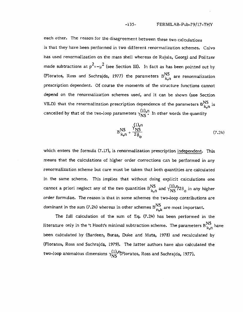
-13% FERMILAB-Pub-79/17-THY
each other. The reason for the disagreement between these two calculations
is that they have been performed in two different renormalization schemes. Calvo
has used renormalization on the mass shell whereas de Rujula, Georgi and Politzer
made subtractions at p*=-u* (see Section III). In fact as has been pointed out by
(Fl oratos, R oss and Sachrajda, NS 1977) the parameters Bk,n are renormalization
prescription dependent. Of course the moments of the structure functions cannot
depend on the renormalization schemes used, and it can be shown (see Section
VI1.D) that the renormalization prescription dependence of the parameters Bysn is (l),n
’ cancelled by that of the two-loop parameters yNs . In other words the quantity
4 l),n
BNS NS k,n + ?r$-
0 (7.24)
which enters the formula (7.17)) is renormalization prescription independent. This
means that the calculations of higher order corrections can be performed in any
renormalization scheme but care must be taken that both quantities are calculated
in the same scheme. This implies that without doing explicit calculations one
cannot a priori neglect any of the two quantities B ‘;i”, and YNS (l),?* B ’ o in any higher
order formulae. The reason is that in some schemes the two-loop contributions are NS dominant in the sum (7.24) whereas in other schemes B n k are most important. ?
The full calculation of the sum of Eq. (7.24) has been performed in the NS literature only in the ‘t Hooft’s minimal subtraction scheme. The parameters B k n have ’
been calculated by (Bardeen, Buras, Duke and Muta, 1978) and recalculated by
(Floratos, Ross and Sachrajda, 1979). The latter authors have also calculated the
two-loop anomalous dimensions y,, (‘),TFloratos, Ross and Sachrajda, 1977).
-136- FERMILAB-Pub-79/17-THY
We shall now outline the procedure for the calculation of the parameters
BNS k n and subsequently prove the renormalization prescription independence of the
sun: in Eq. (7.24).
C. Procedure for the Calculation of BFsn ’ We first notice that in order to find B’;i”, as defined in Eq. (7.14)) it is
sufficient to calculate C trn(Q2/p2, g*) in perturbation theory to order g* and put
Q* = p2. This is obvious from Eqs. (7.10) and (7.11). In order to calculate
C;;n(Q2/v2, g*) in perturbation theory we proceed as follows. We write first the
1.h.s. of Eq. (3.54) as
T&Q*, v) = 1 + n x
+d 1-I vT*,n (7.25)
where p* is the target momentum squared and we have indicated on the r.h.s. of
Eq. (7.25) that TL n, T2 n and T3 n will be calculated in perturbation theory. The ? ’ ’
tensors e and d PV I.lV.
are defined in Eqs. (2.2) and (2.3) respectively. Restricting
the discussion to the non-singlet contributions, we obtain by comparing (3.54) and
(7.25) the following relation for each n separately
C;;$,g*) A;‘($,g’) k=L,2,3 . (7.26)
We observe that in order to find CNS k,$Q h 9 g ) * * * we generally have to calculate
both Tfl and ANS. We have mentioned before that the matrix elements of local ’ n
operators between hadronic states are incalculable in perturbation theory.
Fortunately, the coefficient functions of operators do not depend on the states
-137- FERMILAB-Pub-79/17-THY
between which the operators are sandwiched, and, therefore, in the problem under
investigation we can choose any state for which perturbative calculations can be
performed. Consequently, in Eq. (7.26) T’;i”, are to be found from the virtual ? Compton scattering off quarks and A:’ stands for the matrix element of the spin n
non-singlet operator between quark states. In order to avoid mass singularities in
what follows, we shall keep the external quarks at space-like momenta p* < 0.
where
Next we expand the elements of Eq. (7.26) in a perturbation series as follows
ln d + A(,~),NS P2 I
t
1 k = 2,3 hk =
0 k=L
(7.27)
(7.28)
(7.29)
(7.30)
and the coefficients of the logarithms are fixed by the renormalization group
NS equations which C k n ’
and A:’ have to satisfy (see Section III). In order to simplify
k the notation we have dropped the overall factors 6 NS.
Inserting Eqs. (7.27-7.29) into (7.26) and comparing the coefficients of g* we
obtain
-138- FERMILAB-Pub-79/17-THY
BNS k,n =
(2),NS Tk,n
_ A(*),NS n
To 2 ,NS bn
k = 2,3
k=L . (7.31)
(2) NS We shall comment on the details of the calculation of Tk n’ , A(2)?NS and n BNS
9 k n ’ in Section VI1.E and turn now to a discussion of the renormalization
prescription dependence of BNS k n and of its CanCellath by the renormalization 9 (l),n scheme dependence of the two-loop anomalous dimensions yNs .
D. Renormalization Prescription Independence of Higher Order Corrections
Here we follow the proof of (Floratos, Ross and Sachrajda, 1977).
Consider two renormalization schemes a and b in which the matrix elements
of the operator Ois calculated to order g* are normalized differently as follows
(we drop the index NS)
and
Acp)( $,g*) = AZ [ I+-$ ($$$ln$ +rn)] . (7.33)
(7.32)
Here A: are the zero loop matrix elements which are obviously the same in both
schemes. In scheme a, at p* = -u* the renormalized matrix element An (a) - 1s equal
to the zero loop matrix element. This is a very common renormalization scheme.
In scheme b we have
-139- FERMILAB-Pub-79/17-THY
A;‘(-1, g*) = A0 n [l+srn] (7.34)
where r n are non-zero numbers specific to a given renormalization scheme. In
particular, ‘t Hooft’s minimal subtraction scheme (‘t Hooft, 1973) falls into the
class of b schemes.
Since T(*) k n are independent of renormalization scheme (the virtual .Compton
amplitude is finite and no renormalization is required) we have from Eqs. (7.31)-
(7.33) 1 Bb)
k,n - ‘n k = 2’3 ,(a)
k,n = B(b)
L,n k=L
. (7.35)
Thus B2,n and B3,, are renormalization prescription dependent, whereas BL n is ’
independent of renormalization scheme.
Recall next that
o&n = Zion i = a,b (7.36)
where Oopn * is the bare operator. From (7.32) and (7.33) we have therefore the
following relation between the renormalization constants Za and Zb
za =
Since the anomalous dimension of the operator 0” is defined by
.
n Yi log ‘i 1
Bare quantities fixed i = a,b
(7.37)
(7.38)
-140- FERMILAB-Pub-79/17-THY
we obtain from (7.371, (7.38) and the definition of the f3 function, e.g. Eq. (3.37),
the following relation between yi and yf:
Y: = vf: + *rnSO L (16n21*
or equivalently
(l),n yb
= y (1) a 4 + 2rnSo
Equations (7.35) and (7.40) taken together lead to
y(lh ,ta) + w&-
k,n 2B 0 = B(kb)n
’ +28, k = 2,3
(7.39)
(7.40)
(7.41)
i.e. the combination (7.24) is independent of renormalization scheme. F32
Just before Eq. (7.35) we stated that (2) Tk n are independent of the 9
(2) renormalization scheme. On the other hand it is obvious that Tk n depend on the ’ assumptions about the “quark target” used to extract the coefficient function. In
the discussion above we concentrated on a class of calculations in which the “quark
target” is massless with space-like momentum p* < 0. One could equally well
0) consider massive quarks with p* = 0, In that case Tk n would be different from the ’ (2) case considered here. Also An in a given renormalization scheme depends on the
(2) target (the state between which On is sandwiched). The dependences of Tk n and ’ A(*) n on the “quark target” cancel, however, in the calculation of Bk n as should be ’ the case. We shall illustrate this with an example in Section VIII. It is important to
keep in mind the points discussed in this Section when comparing various
calculations in the literature.
-141- FERMILAB-Pub-79/17-THY
E. Results for y$-‘” and Bzsn 9
(l),n As we have stressed several times one has to make sure that yNs and Btsn 9
are calculated in the same renormalization scheme in order that a physical answer
for the moments of structure functions is obtained. The calculation of the two-
(114 loop anomalous dimensions y NS NS is much more involved than that of B k n and ’
therefore it is useful to choose a renormalization scheme in which the calculation
of ,(l$n - N is simplest. The minimal subtraction scheme of ‘t Hooft, which we have
discussed in Section III, turns out to be a convenient scheme for this purpose.
(l),n 1. Two-loop anomalous dimensions y NS
It has been shown by (Floratos, Ross and Sachrajda, 1977) that in the
‘t Hooft’s renormalization scheme the two-loop anomalous dimensions can be simply
obtained from the coefficient of the l/c pole in the quark matrix element of the
nonsinglet operator calculated tc order g4, plus twice the two-loop anomalous
dimension of the quark field. The latter anomalous dimension is also obtained in
the ‘t Hooft’s scheme by calculating to order g4 the coefficient of l/c pole in the
quark self -energy. Typical diagrams for these two calculations are shown in Figs.
24 and 25. In the whole there are about 30 two-loop diagrams which one has to calculate
(l),NS in order to obtain yNS . All these diagrams have been calculated in the paper by
Floratos, Ross and Sachrajda where the interested reader can find the details of the F3
calculation. + he (l),NS analytic expressions for y n as given in the original paper is
very complicated. (l),n A simpler formula for yNs can be found in the paper by
( Gonzalez-Arroyo, et al., 1978). The numerical values for y(nl)yNS are given in
(lb Table 3. We would like to remark that y NS in the minimal subtraction scheme
are gauge independent (Caswell and Wilczek, 1974).
-142- FERMILAB-Pub-79/17=THY
2. Brsn in ‘t Hooft’s scheme (electromagnetic currents)
The first calc:lation of B”;1”, in the minimal subtraction scheme has been ’
done by (Bardeen, auras, Duke and Muta, 1978). Contrary to the calculation of the
two-loop anomalous dimensions, the calculation of B NS k n in the scheme in question is ? generally more complicated than in other schemes. The reason is that in the
‘t Hooft’s scheme the g* corrections to the matrix elements of local operators
A(*),NS n are non-zero and must be explicitly calculated in addition to the g*
corrections to the virtual Compton amplitude.
The calculation of the virtual Compton amplitude for scattering off quarks in
g* order involves the diagrams of Fig. 26. The diagrams contributing in g* order to
the matrix elements of non-singlet operator between quark states are shown in Fig. 8F34 . Explicit expressions for 70 z ,‘,Ns and A (*),NS
n can be found in the original paper. ’
Here we only remark that although 70 i hNs and p,(*),NS n are separately gauge
’ dependent the resulting expression for BNS ’ 2
’ n IS gauge independent as expected in the
minimal subtraction scheme. We have
n 1 c j=lT
n, even
41 1 3 +4 L- e -+n +(A +$-9 ’ s=ls j=lJ
+TYNS ‘+(ln 4’ - y E)
and
BNS L,n - :” (A -- n even .
(7.42)
(7.43)
The last result for BNS L n which is renormalization prescription independent has been 9 previously obtained by other authors (Zee, Wilczek, Treiman, 1974; Kingsley, 1973;
-143- FERMILAB-Pub-79/17-THY
Walsh and Zerwas, 1973). Recently the calculation of B!sn in the minimal , subtraction scheme has been repeated by (Floratos, Ross and Sachrajda, 1979) who
have reproduced the results of Eq. (7.42).
For the calculations of BNS . 2 n m renormalization schemes different from that 9
considered here we refer the reader to the papers by (Calvo, 1977; De Rujula,
Georgi and Politzer, 1977a;Altarelli, Ellis and Martinelli, 1978; Kubar-And& and
Paige, 1979; Abad and Humpert, 1978 ).
3. BNS . k n in the It Hooft’s scheme (weak currents) ’ In the evaluation of g* corrections to v and < deep-inelastic scattering it is
convenient to consider certain combinations of v ,v structure functions which have
simple properties under crossing. These are
and
FF + FuP 2
F;p - F3”P
F;p + FyP .
(7.44)
(7.45)
(7.46)
(7.47)
The remaining structure functions for scattering off neutron or nuclear targets can
be directly obtained from (7.44)-(7.47) using charge symmetry. For instance
-144- FERMILAB-Pub-79/17-THY
$p _ F;P = F;” 2
-F”p = Fip-Fzn 2 . (7.48)
In order to calculate g* corrections to F *, one considers again the diagrams of Figs.
8 and 26 except that now the diagrams with both vector currents replaced by
axial-vector currents also contribute. The combinations (7.44) and (7.45)
correspond to subtracting and adding crossed diagrams of Fig. 26, respectively.
The structure function F3 corresponds to the vector-axial-vector interference
and therefore the diagrams contributing to it are obtained from Fig. 26 by
replacing one of the vector currents by an axial vector current. Again the
calculation of the gL corrections to the combinations (7.46) and (7.47) corresponds
to subtracting and adding crossed diagrams respectively.
By inspecting the diagrams directly or by considering the decomposition (3.51)
and taking into account known properties of various structure functions under the
transformations u + v , x * -x one can easily find whether even or odd spin
operators contribute to each of the combinations (7.44-7.47). It turns out (Bailin,
3-v Love, Nanopoulos, 1974; Politzer, 1974) that to F2 and Fp only odd spin and to ,>”
2 and Fy-’ only even spin operators contribute.
Finally we have to determine which combinations are independent of gluon
operators, and therefore satisfy simple renormalization group equations as given in
Eq. (4.8). The combinations (7.44) and (7.46) transform obviously as non-singlets
under flavor symmetry and therefore satisfy equations like (4.8). Fjp + F;p is a
singlet combination as discussed in Section II. Therefore because of mixing
between gluon and fermion singlet operators this combination will satisfy more
complicated renormalization group equations, which we shall discuss in Section VIII.
On the other hand, FF” still satisfies Eq. (4.8) in spite of having contributions
-14% FERMILAB-Pub-79 / 17-THY
from singlet fermion operators. This is because the gluon operators of odd spin
transform differently under charge conjugation than the corresponding singlet
fermion operators and therefore there is no mixing.
In the minimal subtraction scheme the results for the parameters Bk n 7
relevant for v, 7 scattering are as follows (Bardeen, Buras, Duke and Muta, 1978)
BF-U 24
= By’, ,
,3-v Ln = Bysn
9
B;‘v _ BNs -3 ‘%I+2 3,n - 2,n 3 ni
9 n odd
n odd
(7.49)
n odd - n even . (7.51)
where BySn and Bysn 9 9 are given by (7.42) and (7.43) respectively. Result (7.50) has
been previously obtained by (Zee, Wilczek, and Treiman, 1974). For the calculation
of B$ in different renormalization schemes from those considered 9 and ByiU I
here we refer the reader to the papers by (Calvo, 1977; Altarelli, Ellis and
Martinelli, 1978).
4. Corrections to sum rules and parton model relations
It is well known that in the leading order of asymptotic freedom parton model
-2 relations and sum rules are satisfied. The g corrections discussed in this section
can generally introduce violations of the sum rules and relations in question.
Notice in particular that the g2 corrections to the Q2 dependence of F3(x, Q2)
differ from the corresponding corrections for F2(x, Q2).
Evaluating formulae (7.49)-(7.51) for n = 1 and recalling that y\S = 0 for n = 1
due to current conservation one obtains corrections to the Gross-Llewellyn-Smith
-146- FERMILAB-Pub-79/ 17-THY
sum rule (Gross and Llewellyn-Smith, 1969) and the Bjorken sum rule (Bjorken,
1967) as shown in Eqs. (2.99) and (2.100) respectively. In Fig. 27 we have plotted
predictions of Eqs. (2.99) and (2.100) versus Q2/A2. We observe that the
deviations from the two sum rules in question are predicted to be non-negligible
and accurate measurements should detect them.
We defer the discussion of QCD corrections to the Callan-Gross relation (Eq,
2.43) to Section VIII.
F. Phenomenology of the Order g2 Corrections (Non-singlet Case)
In this section we shall compare the formula
MNS(n Q2) k -NS k ’ = ‘NSAn I [ 3 lnQI.
-d”NS
A2 (7.52)
with experiment (Bardeen, Buras, Duke and Muta, 1978). The only free parameters
-NS in Eq. (7.52) are the constants An and the scale parameter A. These parameters
are to be found by fitting the formula (7.52) to the data for as large a range of Q2
as possible.
As we have discussed in Section VII.A, there is freedom in defining the
effective coupling constant and, correspondingly, the parameter A. The A which
NS NS enters Eq. (7.52) corresponds to R k,n given by Eq. (7.17) with Bk n calculated in 9 ‘t Hooft’s wjlnimti scheme and to the following form of g2(Q2)
= 1
B, In T2
Bl
7 0
2 In In F2
11
in2 QZ A2
1
ln3 2 A2
(7.53)
-147- FERMILAB-Pub-79 /17-THY
Clearly this definition of A is not unique, and we shall now discuss other possible defi-
nitions.
The effect of the redefinition of A is equivalent through order g2(Q2) to the
shift of RFyn(Q2) by a constant amount proportional to the one-loop anomalous
‘@ dimension y NS . In fact resealing A in Eq. (7.52) to A’ by
A = KA’ (7.54)
where K is a constant, and dropping terms of order $(Q2) generated by this
resealing one obtains
MNS(n Q2) = d k ANS k ’ NS n ’ J
B,ln y, . A2
L I
where
R’;;n(Q2) = R;yn(Q2) + y$n K .
? -l
. (7.55)
(7.56)
The A’ thus corresponds to the s” corrections given by Eq. (7.56) and g’(Q’) having
the form of Eq. (7.53) with A replaced by A’.
It should be remarked that Eqs. (7.52) and (7.55) are equivalent represen-
tations of next to the leading corrections. On the other hand they correspond to
different estimates of the higher order terms 0 g (Q2)) not included in the analysis. r
This is obvious, since in going from Eq. (7.52) to (7.55) we drop terms of O@(Q2)).
It should be remarked that since the n dependences in Eqs. (7.52) and (7.55) are
-148- FERMILAB-Pub-79/17-THY
different from each other so will be the free parameters Afs and A extracted in
both cases. However if the estimates of terms of O(2) by Eqs. (7.52) and (7.55) are
not very different from each other, the equations in question should give equally
good fits to experimental data. To illustrate this we have compared two different
schemes for h with data of BEBC for the moments of Fi (Bardeen et al., 1978).
The first scheme we call the minimal subtraction scheme, and we denote the
corresponding value of A by AMS. This scheme is defined by Eq. (7.52) with A
replaced by ~~~ The second scheme is defined by choosing in Eq. (7.54)
K = exp [ -Yz(ln HIT - y E) 1 . (7.57)
We shall denote the corresponding h by Am Effectively (see (7.55)) the MS
scheme is represented as the MS scheme by Eq. (7.52), but with A replaced by AK
and Rf$,(Q’) replaced by R k n -Ny (Q2) which is given as follows
E;sn(Q2) = RFsn(Q2) - K y $f(ln 4?~ - y E) . 9 9 (7.58)
Recalling Eqs. (7.17) and (7.42) we observe that the MS scheme does not involve the
terms (In 4n - YE). The comparison of these two schemes for A with the BEBC data
leads to the following values for hMS and Am
A MS = 0.40 GeV
hKE = 0.52 GeV (7.59)
-149- FER?iIILAB-Pub-79/17-THY
In obtaining these values, Nachtmann moments of Eq. (2.123) have been used. The
fits to the data are indistinguishable from each other and are represented in Fig. 28
by a single curve. The leading order prediction (not shown in the figure)
My%, Q2) ILo -4A
with
A Lo = 0.73 GeV .
(7.60)
follows very closely the solid line of Fig. 28. We shall discuss below more sensitive
ways of comparing higher order predictions with the 1 eading order results.
We recall that in fitting the data both A’s and An’s have been treated as free
parameters. Therefore the fitted values of the uncalculable matrix elements An’s
are different for different schemes. The similarity of the LO, IMS and MS fits
simply indicates that it is possible for the An’s and >- in each case to conspire to
mask the combined n- and Q2-dependence of the order g2 corrections. Of course
the similarity of the fits of higher order corrections (MS and MS schemes) and of
leading order predictions is, strictly speaking, only true over some not too large
range in Q2 as is the case for the presently available data.
It is instructive to calculate the term
(7.61)
I+ Rag,
L) (7.62)
-150- FERMILAB-Pub-79/17-THY
in Eq. (7.52), which is equal unity in the leading order. The numerical values for
the quantity (7.62) are given for the MS and MS schemes in Table IV. We observe in
accordance with earlier expectations (Gross, 1974; Gross, Wilczek and Treiman,
1976) that, for large values of n and for not too large values of Q2 higher order
corrections are large and perturbative calculations cannot be trusted. This NS behavior is mainly due to the constants B k n which for k f L grow like (In n)2. We
9 observe also that the terms (7.62) are much smaller in the MS scheme as compared
to the MS scheme. The MOM scheme of Table IV is discussed in Section VI1.H.
As we already discussed above some part of the effects due to higher order
corrections in the second term in Eq. (7.52) can be absorbed over a not too large
range of Q2 in the (incalculable by present methods) hadronic matrix elements of
local operators. This makes the phenomenological study of higher order corrections
in deep-inelastic processes complicated. We shall see in Section IX that the
situation is much better in photon-photon scattering where
expression and the next to the leading order predictions
the leading order
are free of the
incalculable matrix elements of local operators.
The values of A as given in Eqs. (7.59) and (7.61) have been obtained for f = 4
and without taking quark mass effects into account. At low values of Q2 (few
GeV2), the massless approximation is probably justified for the light quarks, but not justi-
fied for the charm quark contributions. The effect of heavy quark masses (in the B function)
for the extraction of the value of A in the analysis with higher order corrections
included has been recently studied by (Abbott and Barnett, 1979), who find the
values of A ,which are smaller by roughly 20% than those in Eqs. (7.59) and (7.61).
We think that heavy quark mass effects deserve further study.
-151- FERMILAB-Pub-79/17-THY
G. A, Schemes
As we discussed at the beginning of this section, if the coefficient of
l/(B,ln Q2/A2) in Eq. (7.52) were independent of Q2 and had exactly the same n
dependence as yI($, then all g2 corrections could be absorbed in the parameter A,
and the higher order formula would look like the leading order expression.
Conversely, we could say that the leading order formula assumes that the next-to-
leading order corrections have the same n dependence as the yI($. Therefore it is
of interest to see whether the next-to-leading order corrections, which we have
calculated in this Section, exhibit a non-trivial n-dependence different from yiin.
To this end it is useful to cast Eq. (7.52) into a different form (Bate, 1978; Bardeen
et al., 1978). One can, for instance, (Bardeen et al., 1978) perform the integral in
Eq. (7.10) exactly using y :S and B(g) of Eqs. (7.12) and (7.13), respectively, and
define an n-dependent An as follows F35
h 04 n
This leads to
MFS(n, Q2) = d ks$Is
n
where j$ satisfies the following equation
,(l),n
24 - d”Ns ii2 n
16n2
(7.63)
-I d”Ns 1 . (7.64)
(7.65)
-152- FERMILAB-Pub-79/17-THY
It turns out that the factor involving y i$” ’ in Eq. (7.64) is always very near unity
in the region of interest, hence Eq. (7.64) has essentially the same form as the
leading order Eq. (7.60). Therefore the difference between the leading order and
the higher order corrections, so far as the n dependence is concerned, resides
(k) -NS almost entirely in the scale A,, . Notice that if B k n were proportional toy Ovn, 9 NS
A(k) n would be independent of n. There is one weak point in the An scheme discussed
above. Although MFS(n, Q2) is renormalization-prescription independent, An as
defined in Eq. (7.63) depends on the renormalization scheme through gFsn. 7
Similarly, the third factor in Eq. (7.64) depends on the renormalization scheme
through ~51’~~ -NS s l
Fortunately, in the ‘t Hooft’s scheme the B k n give the dominant 9
contribution to the higher order corrections and the third factor in Eq. (7.64) is
close to unity. Therefore, in the ‘t Hooft’s scheme discussed here, the A:’ as
defined in Eq. (7.63) is a useful quantity for testing the n dependence of the higher
order corrections. It should be kept in mind, however, that one can find
renormalization schemes in which the main n dependence of higher order
(lb corrections resides in yNs ; in this case A:) of Eq. (7.63) would be useless for
testing the higher order corrections.
04 In order to compare the n-dependence of h n with the data, one fits
MF’(n, Q2) as given by Eq. (7.64) to the data for each n separately and extracts in
this way the experimental values for An. It turns out (Bardeen et al., 1978) that for
n < 5 the n dependence predicted by formula (7.63) is in fair agreement with the
BEBC data for F3 (Bosetti et al., 1978). For higher values of n the BEBC data do
not agree with Eq. (7.63). Recently the analysis in question has been repeated by
(Duke and Roberts, 197%) who also took into account the CDHS data for F3
(de Groot et al., 1979a)and Fermilab (Gordon et al., 1978) and SLAC data for Fg-“.
A similar analysis has been carried out in a slightly different way by (Andersson et
-153- FERMILAB-Pub-79/17-THY
al., 1979). It follows from the analysis of Duke and Roberts (see Fig. 29 F %at there
is remarkable agreement of formula (7.63) with the data for F$-” and agreement
for low n with the CDHS data for F3. We may conclude that there are indications
in the data for the n dependence of An as predicted by QCD.
A comparison of the higher order prediction (7.52) and the leading order
prediction (7.60) can be done in a simpler way than discussed above, at the price of
introducing a weak Q2 dependence into An. The method discussed below is very
similar to that proposed by (Bate, 1978).
Eq. (7.52) can be written as follows
MN% Q2) k ’ = 6 k $S
NS n
where
-d”NS (7.66)
A(kJtQ2) _ 7 exp ‘!!?n(Q2) n -1 1 04 . (7.67)
’ NS
Now the difference between the leading order and higher order corrections resides
t totally in A,(Q’). U A ex using Eqs. (7.17) and (7.21) we can write
Ank)(Q2) = ii Z,(Q’,h ) (7.68)
where
Zn(Q2, 71) = [ T2] -8l’28’ exp [ 2ifiLn ---J ] exp [s] . In 2 (7.691 0
-154- FERMILAB-Pub-79/17-THY
Notice that the first factor on the r.h.s. of Eq. (7.69) represents the Q* evolution of
(k) 2 An (Q ). The second factor, on the other hand, introduces additional n dependence
04 as compared with the An scheme of Eq. (7.63). Since this additional n dependence
(a 15% decrease from n ‘k) 2 = 2 to 10) is very weak, the n dependence of AA (Q ) is
(k) essentially the same as that of An , which changes roughly by a factor 2 over the
range from n = 2 to 10. The Q2 dependence of the first factor in Eq. (7.69) is such
that for f = 4 and x = 0.3 and x= 0.5, at Q2 = 100 GeV’, Z&Q’, 7) is suppressed by
the factors 1.23 and 1.29, respectively.
In summary, the ALk)(Q2)scheme as defined by Eq. (7.66) is (except for the
(k) overall factor) quite similar to the An scheme of Eq. (7.64), but very accurate
experiments should detect the Q2 dependence as predicted by Eq. (7.69). In Fig. 30
we have shown Aj12)(Q2) for ? = 0.5 and f = 4 as functions of n and Q2. For
comparison we plot the last factor in Eq. (7.70) which represents the An gcheme. (k It
(k) 2 should be remarked that An (Q ) in Eq. (7.67) is renormalization-prescription
independent.
Finally we would like to remark that (Anderson et al., 1979) have extracted
,+2) (2) 2 n using the formula (7.66) and neglecting the Q2 dependence of An (Q ). Their
results agree very well with Eq. (7.63). In order to test the Q2 dependence of
(2) 2 An (Q ) as given by (7.67) one should repeat Anderson’s analysis in various ranges
of Q2, e.g. 2-5 GeV’, 5-10 GeV’, LO-30 GeV’, etc. The prediction of the theory is
(2) that for a fixed n value a slow decrease of An with increasing Q2 should be
observed. The present data are however not accurate enough to detect this Q2
dependence. Notice that the Q2 dependence in question is entirely due to the two-
loop contributions to the 6 function.
-155- FERMILAB-Pub-79/17-THY
H. Other Definitions of c2(Q2)
In the previous subsections we have discussed the MS and MS schemes for the
effective coupling constant. The corresponding parameters RySn 7 and l?:Sn are
9 related to each other by Eq. (7.58 ) and the numerical values of the quantities of
Eq. (7.62) for these two schemes are collected in Table IV. We observe that in the
expansion in the inverse powers of logarithms the next-to-the-leading order
corrections to MF’(n, Q2) are smaller in the MS scheme than in the MS scheme.
Generally one can introduce other definitions of g2(Q2) for which the parameters R
are related to the corresponding parameters of the MS and MS scheme as follows
= I$“,- 9
K y$J(a - 1.95) .
Here a is a constant, which distinguishes between various schemes and
1.95 = In; 4WYE. In particular Barbieri et al. (1979) and Celemaster and Gonsalves
(1979) have discussed g2(Q2) as defined by momentum space subtraction. The -2 2 g (Q ) so defined is gauge dependent but the gauge dependence is very weak.
Cel emaster and Gonsavles have used the Landau gauge for which a = 3.5. The case
discussed by Barbieri et al. corresponds to a = 3.6. We observe that in both cases
the parameters R are smaller than in the MS and MS schemes. One could conclude
from this that the next-to-the-leading order corrections in the schemes based on
momentum subtraction are smaller than in the MS and MS schemes. However in
order to be able to draw any conclusion one has to determine first from experiment
the values of A for momentum subtraction schemes. We have made the following
-156- FERMILAB-Pub-79/17-THY
exercise. We took x = 0.50 GeV extracted from the BEBC data and ‘E; = 0.30 GeV a
value more relevant for the CDHS data and calculated the moments My’(n, Q~) in
the MS scheme for these two cases. Next we found the values of A mom
(momentum subtraction) by fitting the moments M2 NS(n, Q2) calculated in the
momentum subtraction scheme with a q 3.5 to the moments M2 NS(n, Q2) calculated
in the E scheme. For 7~ 0.50 GeV and n = 0.30 GeV the corresponding values of
A mom turn out to be Amom = 0.85 GeV and Amom = 0.55 GeV. The effective
coupling constants in the three schemes considered for A = 0.40 GeV, n= 0.50 GeV
and A mom q 0.85 GeV are plotted in Fig. 31. We observe the following inequalities
which correspond to
RNS 2,n > l+j; > RySn I,,,. Furthermore we observe that in all cases considered 9 9
the effective coupling constant is smaller than that given by the leading order
expression. The numerical values of the quantities of Eq. (7.62) for the three
schemes are shown in Table IV. We conclude that in the expansion in the inverse
powers of logarithms the next-to-the-ieading order corrections to MyS(n, Q2)
calculated in the momentum subtraction scheme with a = 3.5 are larger than those
in the MS scheme but smaller than in the MS scheme.
In spite of this analysis we cannot say which of the schemes considered leads
to the best convergence of the perturbative series. In order to be able to answer
this question one would have to calculate higher orders in g2(Q2) not included in the
analysis. Needless to say the n dependence of An(Q2) or An discussed in the
previous subsection is independent of the definition of z2(Q2).
-157- FERMILAB-Pub-78/17-THY
VIII. HIGHER ORDER ASYMPTOTIC FREEDOM CORRECTIONS TO DEEP-INELASTIC SCATTERING (SINGLET CASE)
A. Preliminaries
In the last section we have discussed next-to-leading asymptotic freedom
corrections to the moments of the non-singlet contributions to the deep-inelastic
structure functions. In this section we shall extend the analysis to the singlet
contributions. Such an analysis requires the calculation of the two-loop anomalous
dimension matrix and of the one-loop corrections to the fermion singlet and gluon
Wilson coefficient functions. As in the non-singlet case, one has to take care that
all these quantities are calculated in the same renormalization scheme. In the
minimal subtraction scheme one-loop corrections to the fermion singlet and gluon
Wilson coefficient functions have been calculated by (Bardeen, Buras, Duke and
Muta, 1978) and by (Floratos, Ross and Sachrajda, 1979). The latter authors have
also computed the two-loop anomalous dimension matrix. The study of the next-to-
the-leading corrections in the singlet sector is complicated by the mixing of gluon
and fermion singlet operators. The problem of mixing for the next-to-the-leading
order corrections was first solved by (Floratos, Ross and Sachrajda, 1979). Here we
shall present an equivalent, but slightly simpler , approach of (Bardeen and Buras,
1979b)F3$ost of our discussion will be rather formal and only at the end of this
section shall we present a parton model formulation of asymptotic freedom beyond
the leading order.
B. Moments of the Singlet Structure Functions
We shall now derive Eqs. (2.101)-(2.117) of Section II. We begin with
F2(x, QL). In the formal approach of Section IV the moments of the singlet part of
F2 are given as follows
-158- FERMILAB-Pub-79/17-THY
h$(n,Q’) : l,i”” x”-~F~~x,Q~) = Ai(u2)C$,n ($ , g’) 1-I
with all symbols defined in Section 1V.A.
The Q2 dependence of the coefficient functions C~,n(Q2/~2, g2) and
C:,n(Q2/p2, g2) is governed by the renormalization group Eq. (4.20) which has the
following solution
~2,n($g2) = [Tgexp ‘,BbZ,d&$$$ ] 52,n(I,i2)
with g(u2) = g. As in Section 1V.C we have introduced here the column vector
E2,n($y 9’) =
m cll’ $,g2 0 ( 1 P2
‘(jn ‘Yg2 Y i 1 u2
(8.2)
. (8.3)
The 2 x 2 anomalous dimension matrix F”(g)- is shown explicitly in Eq. (4.22). It has
the following perturbative expansion
^v “(g) = +n L + $l),n L + ,.. 167~’ (16n2J2
. (8.4)
We shall now express the T ordered exponential in Eq. (8.2) in terms of the
coefficients in the expansions (7.13) and (8.4). Denote first
%g, 9 = Tg exp I- g dp’j$f dQ2)
(8.5)
and write it as
-159- FERMILAB-Pub-79/17-THY
fag, ijl = %g) [ exp($lni)] ?‘(a (8.6)
where G(g) is a 2 x 2 matrix which we shall now find. To simplify the notation we
shall drop the index n in Eqs. (8.7)-(8.1 I).
Differentiating both sides of Eqs. (8.5) and (8.6) with respect to g we obtain
respectively
agW(g,a = @J t(g) exp A0 c 3 ;f- I+ iJ-'tj$
0 (8.7)
and
a,WCg, 3 = agv(g) - "v(g) $ $ . (8.8) 0
Equating the r.h.s. of these two equations we obtain after some manipulations the
following differential equation for e(g)
a gi(g) + $ [ $itg,] = (g$ +Eg) i(g)
Writing next
G(g) = ? + AZ- v^ 16~’ ’
where 1 is a unit matrix, we obtain the following algebraic equation for t2
2^v2 + -0 ,-.
1 I $1) FOB1
k’V2 z-B+--- 0 0 62 0
.
. (8.91
(8.10)
(8.11)
-160- FERMILAB-Pub-79/17-THY
AO,n . In order to solve Eq. (8.11) it is useful to choose the basis in which y IS diagonal.
As in Section 1V.C we introduce the matrix U which diagonalizes y Ao9n by
A” 0 b-lp O,nG =
(- )
. (8.12) 0 x” +
A Explicit expression for a U matrix which does this job is given in Eq. (4.30).
In the basis in which yopn ’ A (l),n IS diagonal, the matrices y and G2 are given as
follows
(8.13)
and
Diagonalizing Eq. (8.11) and using Eqs. (8.12)-(8.14) we obtain
y(lh pB -- - 1 -- +- 5- q 28, 28;
+l),n p B
%’ = ii, + 1 --+- 2B2
0
. (8.14)
(8.15)
(8.16)
-161- FERMILAB-Pub-79/17-THY
v;+ = - y (l),n
-+ (8.17)
a3 O+x ;-A:
v;- = - y (lh +- 230+x~-xn
. (8.18)
Explicit expressions for y (l&n, y (l),n, ,(l),n and ,(l),n -- ++ -+ +- are given in Eqs.
(2.109) to (2.112). A s iscussed in Section 1V.C the 6 matrix which diagonalizes d’
T o,n is not uniquely defined by Eq. (8.12), and any other matrix related to ^u by Eq.
(4.29) will also satisfy Eq. (8.12). It follows from this that only the diagonal
elements yO,n, Y(‘),~ (l),n (l),n -- ++ and the product y+- .y-+ are independent of our choice
of fi. Eqs. (2.109)-(2.112) correspond to ?J given by Eq. (4.30).
To proceed further we introduce a column vector
C& <YE2 - Y ( 1 ’ P
G,n ( ). Qf,g2 112
= ^v-lc’ 2,n($,g2) ’
The components C z,,(Q2/p 2, g2) are easily obtained by first writing
ir-‘k2,n( $, g’) = ?‘ii(g, gJ ii-l?52,n(l, i2,
(8.19)
(8.20)
and then using Eqs. (8.61, (8.12)-(8.14). The result is
-162- FERMILAB-Pub-79/17-THY
and
- ‘2,n( .
‘)y putting Q2 = p2 in Eq. (8.19). Furthermore Here Ciyn(l, g2) are obtained k
-_ d ,n cs2
l-l2 1
( 1 $42 1-I
“G,n
where ? a 2,n(Q2/ u29 g2) are given as follows
1 (8.21)
(8.22)
(8.23)
A”+ d:” = 28, . (8.24)
We next expand C zyn( 1, g2) and C: Y n( 1, i2) ’ m a power series in g2 as follows
1+&j+ 16~r~ 2,n (8.25)
and
-163- FERMILAB-Pub-79/17-THY
($Jl, g2) = 6;) if- BG 167~~ 2yn
where 6f) depend on weak and electromagnetic charges. Defining also the
perturbative expansion for C g,,(l, g2) by
(8.26)
C& i2, = C;f 1 + 2 B’ Y 161~’ 2yn 1
we obtain from Eqs. (8.19), (8.25), (8.26) and (4.31)
(8.27)
and the formulae (2.107) and (2.108) for Bz n. Y Equation (8.27) is the generalization
‘of the leading order expression (4.37). With all the formulae above at hand, we
could now perform matrix multiplication in Eq. (8.21), and we would reproduce the
Eq. (2.13) in the paper by (Floratos, Ross and Sachrajda, 1979). In order to obtain
slightly simpler equations we proceed in a different way.
We first write Eq. (8.1) as
(8.28)
Ms(n, Q2) = “An(u2)c’ 2,n($ ,g’)
where $( $) is a two component row vector given by
Ant P2) = [ A;(u’), A;( u2) I
(8.29)
(8.30)
Defining next
-164- FERMILAB-Pub-79/17-THY
1 + 2- ?G,;r ) 161~~
(8.31)
we obtain
M$n, Q2) = ?(u2)e; n Y + A$12)c+ “2,n( ‘tf2 ,g’) (8.32)
with C -2;ntQ2/u2, g2) g’ iven by Eqs. (8.22) and (8.23).
Next using Eq. (7.19) for g2(Q2), we obtain the final expression for the
moments of F2(x, Q2)
M;(n, Q2) = &t2)K- 9 n
R; .(Q2) Y
8, In 2 A2
where
-d;
R;JQ’) = A&
R; n - - Y 4
(8.33)
(8.34)
and the constants Rz Y n are given as follows
T T y (I_)4
R2,n T+ = BZyn +28, -
A& y(l),n
7+
28, + hi - 1; . (8.35)
Anrare constants which are related to ii(u2) by
-165- FERMILAB-Pub-79/17-THY
--T -d;
An = + i’(p2) [ i2(lJ2) ] (8.36)
2 K ’ are independent of u . Equation (8.33) is the generalization of the leading
order formula (4.41b). It should be remarked that K t and Rz n are independent Y
of the choice of the matrix U.
The matrix U of Eq. (4.30) differs from that used in the paper of (Floratos,
Ross and Sachrajda, 1979). However as the interested reader may check y (l),n , -- y(l),n
++ and ,(lh ,(lh
-+ +- are the same as in the paper in question.
Let us brlef!y discuss Eq. !8.33). It is probably the simplest possibie
representation of the next-to-leading order corrections for the singlet structure
functions. We would like to emphasize two important features of Eq. (8.33)
i) no reference is made to a special value of Q2 = Q$ and
ii) no reference is made to the parton distributions.
The property i) has already been discussed in Section IV in connection with the
leading order expressions. It is required by renormalization group equations and
incorporating it in M?Jn, Q2) simplifies phenomenological applications. In particu-
lar the Step 9 of the procedure of Section II can be omitted if Eq. (8.33) is used.
Concerning ii) we would like to recall that the parton distributions cannot be
uniquely defined beyond the leading order of asymptotic freedom (see Section VIIIE for de-
tails). Many definitions are possible, which differ from each other by next-to-leading order
corrections. Therefore the study of higher order effects on the Q’ evolution of quark and
gluon distributions does not make much sense because the result of such a study is not a
prediction of the theory but depends sensitively on one’s definition of parton
distributions. Furthermore equations for the Q2 evolution of parton distributions
-ic&- FERMILAB-Pub-79/17-THY
are much more complicated than Eq. (8.33). Therefore we think that the simplest
and most straightforward tests of higher order corrections can be done directly by
means of Eq. (8.33) and (7.20b) without any reference to parton distributions. Still
with a given definition of parton distributions, the parton language may be useful in
comparing asymptotic freedom predictions in various processes such as deep-
inelastic scattering, Drell-Yan process, etc. Therefore at the end of this section
we shall discuss a parton model formulation of higher order corrections.
After having discussed some attractive features of Eq. (8.33) we should
mention a possible limitation in the use of it. We observe that the last term in the
expression for R;,n in Eq. (8.35) is singular when dy = d_” + 1. While this singularity
does not appear for physical values of n and f, it can lead to anomalously large
higher order corrections to the ‘,-,, contributions and an apparent breakdown of
perturbation theory.
The singularity in R; ,n
is of course spurious and must be cancelled by other
terms in Eq. (8.33). At this stage it should be recalled that A,’ are rather
complicated functions (see Eqs. (8.31) and (8.36)) of the matrix elements of singlet
fermion and gluon operators and of various renormalization group parameters which
we lumped together in order to obtain a simple expression and get rid of lo 2 = Q;
dependence. In doing this we have generated singularities in 5 ,n and AA for non-
integer f and n which cancel each other in the full expression. In fact, on the basis
of Eqs. (8.31) and (8.361, rn can be written as follows
“; = AA + +o (3.37)
where Ai is non-singular and the singularity is in R;’ which is given as follows
-167- FERMILAB-Pub-79/17-THY
R;+ = +n
-+ Y
Qz is an arbitrary scale. Inserting Eq. (8.37) into (8.33) we convince ourselves that
the singularity in Rn is indeed cancelled by that in R;;‘.
From a detailed numerical study of the singularities in %,n (Bardeen and
Buras, 1979b) it follows that only in the case of n = 2 and then only for f = 5 and 6 F3 is the separation of the singular part as shown in Eq. (8.37) necessary. F or all other
physical values of n and f, the existence of a nearby singularity does not disturb the
validity of the perturbative nature of the corrections and Eq. (8.33) can be safely
used.
For completeness however we would like to mention that one can derive an
equation for M52(“, Q2) which, although is slightly more complicated than Eq. (8.33)
and involves explicitly Q$ can be easily continued to non-integer values of f and n.
This is the Eq. (2.1 Ola) which can be easily derived by performing matrix
multiplication in Eq. (8.21), instead of absorbing the first factor on the r.h.s. of Eq.
(8.21) into matrix elements of local operators as was done in the present derivation.
So far we have discussed only F$x, Q2). The formula for the singlet part of
the longitudinal structure function can be derived in a similar way by replacing the
Eqs. (8.25) and (8.26) by
(8.38)
C;,n(l, g22, = gL i?- B’ + 1Ga2 L,n
and
(8.39)
~;,~(l, g2, = 6; z BG 16-rr2 Lyn
(8.40)
The result is
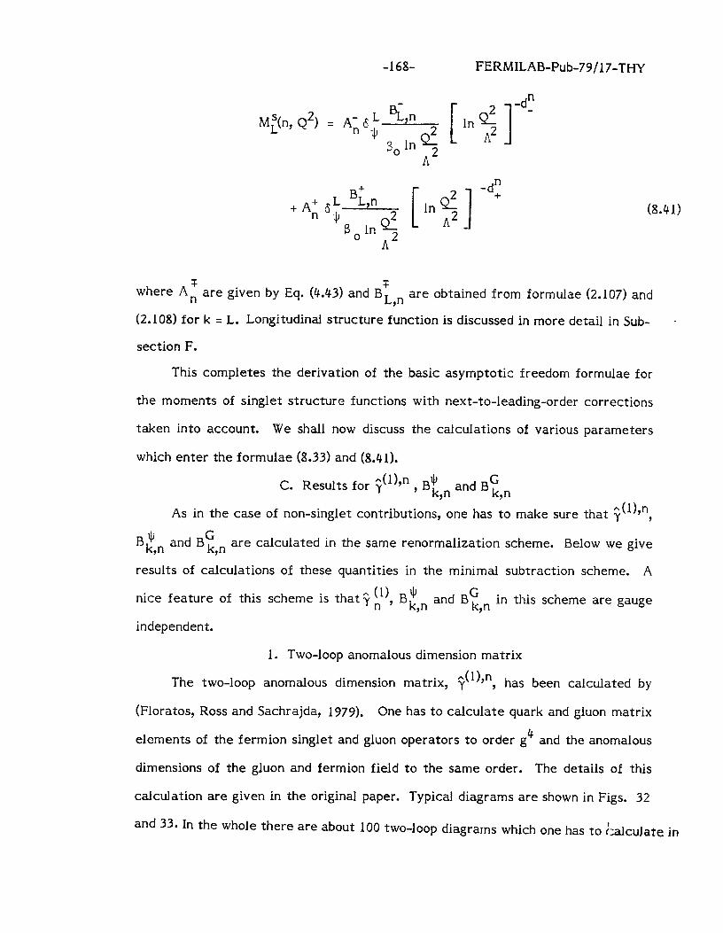
-168- FERMILAB-Pub-79/17-THY
ML(n, Q2) = A- 6 L %,n n 4J
[ 1 InQI
-d;
A2 (8.41)
where AZ are given by Eq. (4.43) and 8: n are obtained from formulae (2.107) and Y (2.108) for k = L. Longitudinal structure function is discussed in more detail in Sub- -
section F.
This completes the derivation of the basic asymptotic freedom formulae for
the moments of singlet structure functions with next-to-leading-order corrections
taken into account. We shall now discuss the calculations of various parameters
which enter the formulae (8.33) and (8.41).
4l),n J, C. Results for y G y Bk,n and B k,n
As in the case of non-singlet contributions, one has to make sure that y A(l),n ,
Btn and Y Bt n Y are calculated in the same renormalization scheme. Below we give
results of calculations of these quantities in the minimal subtraction scheme. A
nice feature of this scheme is that y n , h (1) BlCi G kn and Bkn in this scheme are gauge Y Y
independent.
1. Two-loop anomalous dimension matrix
4l),n The two-loop anomalous dimension matrix, y , has been calculated by
(Floratos, Ross and Sachrajda, 1979). One has to calculate quark and gluon matrix
elements of the fermion singlet and gluon operators to order g4 and the anomalous
dimensions of the gluon and fermion field to the same order. The details of this
calculation are given in the original paper. Typical diagrams are shown in Figs. 32
and 33. In the whole there are about 100 two-loop diagrams which one has to &alculate in
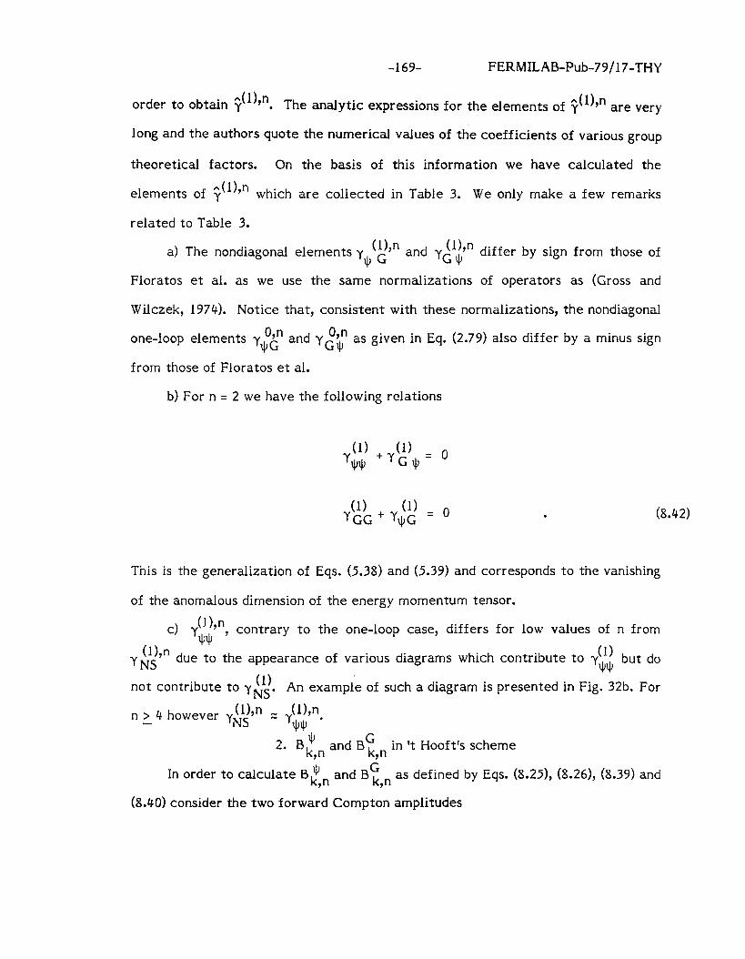
-169- FERMILAB-Pub-79/17-THY
4,n order to obtain y . The analytic expressions for the elements of y A(l),n are very
long and the authors quote the numerical values of the coefficients of various group
theoretical factors. On the basis of this information we have calculated the
A(1)d-i elements of y which are collected in Table 3. We only make a few remarks
related to Table 3.
a) The nondiagonal elements y (1) n (‘)+ and yG $y 4JG
differ by sign from those of
Floratos et al. as we use the same normalizations of operators as (Gross and
Wilczek, 1974). Notice that, consistent with these normalizations, the nondiagonal
one-loop elements y (iin and y&n as given in Eq. (2.79) also differ by a minus sign
from those of Floratos et al.
b) For n = 2 we have the following relations
(1) +yG$= o
. (8.42)
This is the generalization of Eqs. (5.38) and (5.39) and corresponds to the vanishing
of the anomalous dimension of the energy momentum tensor.
cj y(JLn
y f-b w ,
contrary to the one-loop case, differs for low values of n from
due to the appearance of various diagrams which contribute to (1) y 4JQ
but do (1) not contribute to yNs. An example of such a diagram is presented in Fig. 32b. For
(l),n n > 4 however yNs (l),n =: YqJJ, l
dJ G
2* Bk,n and B k,n in ‘t Hooft’s scheme
s In order to calculate Bk n and Bt n as defined by Eqs. (8.251, (8.261, (8.39) and Y Y
(8.40) consider the two forward Compton amplitudes
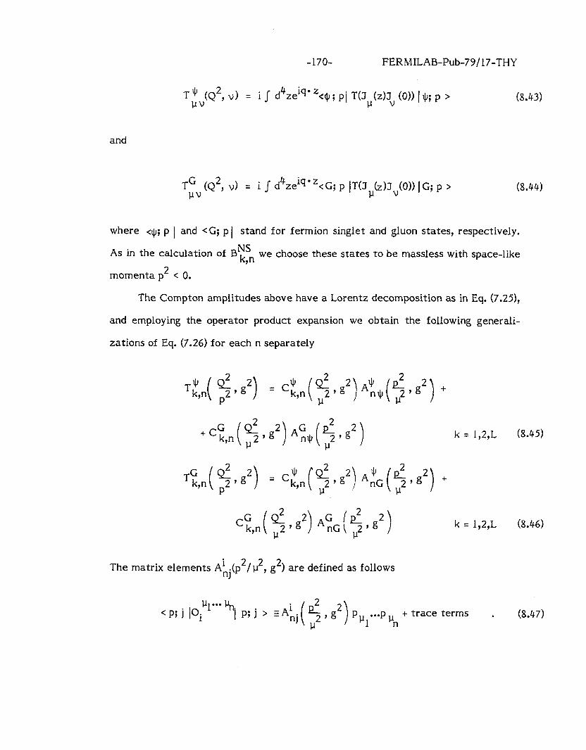
-170- FERMILAB-Pub-79/17-THY
TG (Q2,v) = 4 UV
iJd ze iqo ‘q~ ; pi T(Ju(z)Jv (ON 19; p > (8.43)
and
TFv (Q2, v) = i I d4zeiq l ‘t G; p IT(Jv(z)JV(0)) 1 G; p > (8.44)
where c+; p 1 and <G; p 1 stand for fermion singlet and gluon states, respectively.
As in the calculation of BNS k Y n we choose these states to be massless with space-like
momenta p2 < 0.
The Compton amplitudes above have a Lorentz decomposition as in Eq. (7.251,
and employing the operator product expansion we obtain the following generali-
zations of Eq. (7.26) for each n separately
T;,n( G!zg2) = c:,n($g2)A:@-$2) +
k = 1,2,L
k = 1,2,L
The matrix elements Akj(p2/u2, g2) are defined as follows
< Pi j loi lJ”I”’ “n
P,, *e-P,, + trace terms . 1 n
(8.45)
(8.46)
(8.47)
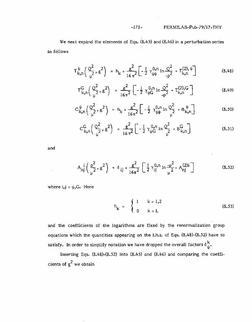
-171- FERMILAB-Pub-79/17-THY
We next expand the elements of Eqs. (8.45) and (8.46) in a perturbation series
as follows
_gs_ = hk+16n2
TG k,n
’ 2
-VljJG Oyn In e + Bi n 3 Y 1
and
(8.48)
(8.49)
(8.50)
(8.5 1)
(8.52)
where i,j = $,G. Here
1 k = 1,2 hk = (8.53)
0 k=L
and the coefficients of the logarithms are fixed by the renormalization group
equations which the quantities appearing on the 1.h.s. of Eqs. (8.48)-(8.52) have to
satisfy. In order to simplify notation we have dropped the overall factors 6:.
Inserting Eqs. (8,48)-(8.52) into (8.45) and (8.46) and comparing the coeffi-
cients of g2 we obtain
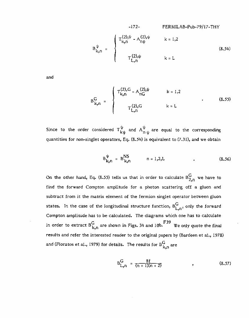
-172- FERMILAB-Pub-79,‘17-THY
GWJ _ A(2)Y$ Tk,n n$ k= 1,2
Bin = (8.54) Y
k=L
and
TfiG _ A k = 1,2 Y
BG k,n = t&G
TL,n k=L
\
. (8.55)
Since to the order considered T$ and A$ krC, “4J
are equal to the corresponding
quantities for non-singlet operators, Eq. (8.54) is equivalent to (7.31), and we obtain
B; n = B;‘, Y Y n = 1,2,L . (8.56)
On the other hand, Eq. (8.55) tells us that in order to calculate Btn we have to Y find the forward Compton amplitude for a photon scattering off a gluon and
subtract from it the matrix element of the fermion singlet operator between gluon
states. In the case of the longitudinal structure function, BE n, only the forward Y Compton amplitude has to be calculated. The diagrams which one has to calculate
G in order to extract B k,n are shown in Figs. 34 and lob. F39
We only quote the final
results and refer the interested reader to the original papers by (Bardeen et al., 1978)
and (Floratos et al., 1979) for details. The results for Bi n are Y
BG 8f Ln = (n + l)(n + 2) (8.57)
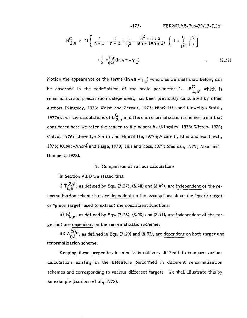
FERMILAB-Pub-79/17-THY
. (8.58)
Notice the appearance of the terms (In 4~ - y E) which, as we shall show below, can
be absorbed in the redefinition of the scale parameter A. Bt n, which is Y renormalization prescription independent, has been previously calculated by other
authors (Kingsley, 1973; Walsh and Zerwas, 1973; Hinchliffe and Llewellyn-Smith,
lP77a). For the calculations of in different renormalization schemes from that
considered here we refer the reader to the papers by (Kingsley, 1973; Witten, 1976;
Calvo, 1976; Llewellyn-Smith and Hinchliffe, 1977a; Altarelli, Ellis and Martinelli,
1978; Kubar -Andre/ and Paige, 1979; Hill and Ross, 1979; Sheiman, 1979 i Abad and
Humpert, 1978).
3. Comparison of various calculations
In Section VI1.D we stated that
i) TF)n ,i Y as defined by Eqs. (7.27), (8.48) and (8.49), are independent of the re- Y normalization scheme but are dependent on the assumptions about the “quark target”
or ,,gluon target,, used to extract the coefficient functions;
ii) BL n, as defined by Eqs. (7.28), (8.50) and (8.51), are independent of the tar- Y get but are dependent on the renormalization scheme;
iii) A::‘, as defined in Eqs. (7.29).and (8.52), are dependent on both target and -¶ renormalization scheme.
Keeping these properties in mind it is not very difficult to compare various
calculations existing in the literature performed in different renormalization
schemes and corresponding to various different targets. We shall illustrate this by
an example (Bardeen et al., 1978).
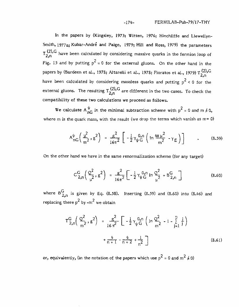
-174- FERMILAB-Pub-79/17-THY
In the papers by (Kingsley, 1973; Witten, 1976; Hinchliffe and Llewellyn-
Smith, 1977a; Kubar-And& and Paige, 1979; Hill and Ross, 1979) the parameters T 6%
2,n have been calculated by considering massive quarks in the fermion loop of
Fig. 15 and by putting p2 = 0 for the external gluons. On the other hand in the
papers by (Bardeen et al., 1978; AItarelli et al., 1978; Floratos et al., 1979) T2(tyG Y
have been calculated by considering massless quarks and putting p2 c 0 for the
external gluons. The resulting T 2(z,),G are different in the two cases. To check the 9
compatibility of these two calculations we proceed as follows.
We calculate A 4J nG in the minimal subtraction scheme with p2 = 0 and m f 0,
where m is the quark mass, with the result (we drop the terms which vanish as m+ 0)
‘x,( $d2) = $2 [ -tY$(+$ -YE)] . (8.59)
On the other hand we have in the same renormalization scheme (for any target)
(8.60)
where B G 2 n is given by Eq. (8.58). ? Inserting (8.59) and (8.60) into (8.46) and
replacing there p2 by -m2 we obtain
4 4 +---,j n+l n+2 1 (8.61)
or, equivalently, (in the notation of the papers which use p2 = 0 and m2 f 0)
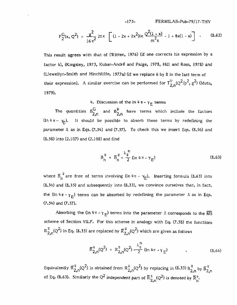
-17% FERMILAB-Pub-79/17-THY
2 F;(x, Q2) = -g- 2f x
161~~ L- (1 - 2x + 2x2)ln G2(l-x)-
m2x 1 + 8x(1 -
x) 1 . (8.62)
This result agrees with that of (Witten, 1976) (if one corrects his expression by a
factor 4), (Kingsley, 1973, Kubar-And& and Paige, 1978, Hill and Ross, 1978) and
(Uewellyn-Smith and Hinchliffe, 1977a) (if we replace 6 by 8 in the last term of
their expression). A similar exercise can be performed for T’ 2,n(Q2/p2, g2) (Mu%
1979).
4. Discussion of the In 4 IT - yE terms
The quantities 2 n and BG Bz n have terms which include the factors 9 9
(In 4 TI - yE). It should be possible to absorb these terms by redefining the
parameter A as in Eqs. (7.54) and (7.57). To check this we insert Eqs. (8.56) and
(8.58) into (2.107) and (2.108) and find
(8.63)
where BnT are free of terms involving (In 4~ - yE). Inserting formula (8.63) into
(8.34) and (8.35) and subsequently into (8.33), we convince ourselves that, in fact,
the (In 4~ - y E) terms can be absorbed by redefining the parameter A as in Eqs.
(7.54) and (7.57).
Absorbing the (In HIT - y E) terms into the parameter A corresponds to the MS
scheme of Section VI1.F. For this scheme in analogy with Eq. (7.58) the functions
Rz .(Q2) in Eq. (8.33) are replaced by Br 9 2,n(Q2) which are given as follows
E!&(Q2) = Rz .(Q*) . 9 (8.64)
Equivalently Rz,,(Q’) is obtained from Rs ,(Q2) by replacing in (8.35) B;n by g:, 9 9 9
of Eq. (8.63). Similarly the Q2 independent part of Ei n(Q2) is denoted by Ei. ?
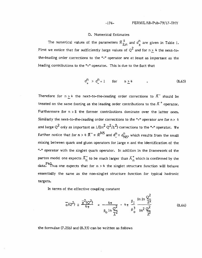
-176- FERMILAB-Pub-79/17-THY
D. Numerical Estimates
The numerical values of the parameters Rtn and d: are given in Table 1. 9
First we notice that for sufficiently large values of Q2 and for nL 4 the next-to-
the-leading order corrections to the ‘I-” operator are at least as important as the
leading contributions to the rl+‘c operator. This is due to the fact that
d: > d” + 1 for n>4 . (8.65)
Therefore for n > 4 the next-to-the-leading order corrections to A- should be
treated on the same footing as the leading order contributions to the K + operator.
Furthermore for n > 8 the former contributions dominate over the latter ones.
Similarly the next-to-the-leading order corrections to the “+‘I operator are for n > 4
and large Q2 only as important as 1/(ln2 Q2/A2) corrections to the “-” operator. We
further notice that for n > 4 R’ z RNS and d” 2 dks, which results from the small
mixing between quark and gluon operators for large n and the identification of the
“-I’ operator with the singlet quark operator. In addition in the framework of the
parton model one expects K-n to be much-larger than x: which is confirmed by the
data. F4?hus one exp ects that for n > 4 the singlet structure function will behave
essentially the same as the non-singlet structure function for typical hadronic
targets.
In terms of the effective coupling constant
(8.66)
the formulae (7,20b) and (8.33) can be written as follows
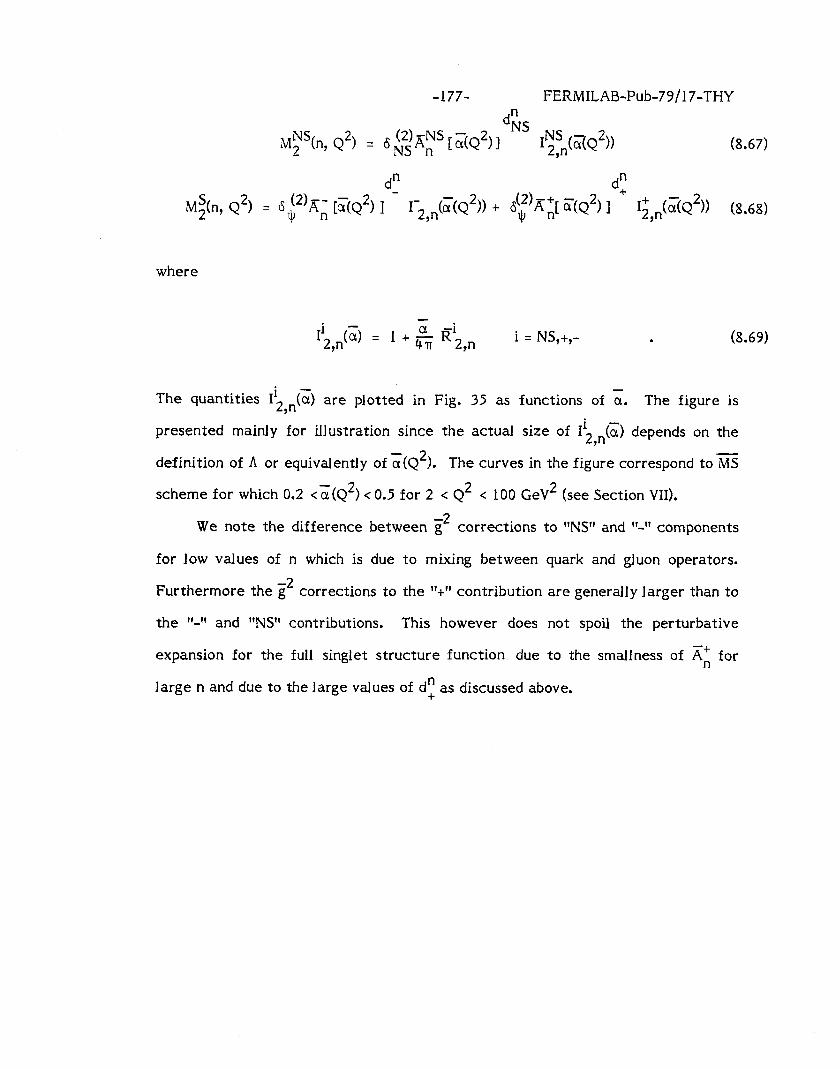
-177- FERMILAB-Pub-79/l 7-THY
&$‘(n, Q*) q 6 ~~$ls 1 ;;(Q2) 1 dF+JS I;$?tQ*)) (8.67)
M$n, Q2) = 6i2)Kn [G(Q2) Id’ I;,,(g(Q2)) + Gti$)K$ z(Q2) Id’ I;,n(?iQ2)) (8.68)
where
Ii2 .(Z) = 1 + & Ri2 n i = NS,+,- 9 9 . (8.69)
The quantities Ii2J-) ~1 are plotted in Fig. 35 as functions of a. The figure is
presented mainly for illustration since the actual size of Ii2n(G) depends on the
definition of A or equivalently of a(Q2). The curves in the figure correspond to=
scheme for which 0.2 <i(Q2) < 0.5 for 2 < Q2 < 100 GeV* (see Section VII).
We note the difference between i’ corrections to ttNS’l and I’-‘( components
for low values of n which is due to mixing between quark and gluon operators.
Furthermore the g* corrections to the I’+” contribution are generally larger than to
the ‘t-1’ and “NS” contributions . This however does not spoil the perturbative
expansion for the full singlet structure function due to the smallness of “i for
large n and due to the large values of dy as discussed above.
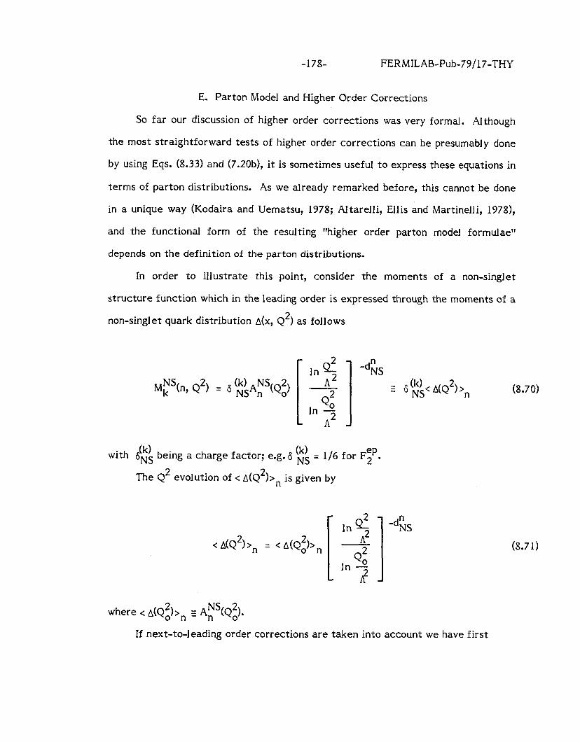
-178- FERMILAB-Pub-79/17-THY
E. Parton Model and Higher Order Corrections
So far our discussion of higher order corrections was very formal. Al though
the most straightforward tests of higher order corrections can be presumably done
by using Eqs. (8.33) and (7.20b), it is sometimes useful to express these equations in
terms of parton distributions. As we already remarked before, this cannot be done
in a unique way (Kodaira and Uematsu, 1978; Altarelli, Ellis and Martinelli, 19781,
and the functional form of the resulting “higher order parton model formulae”
depends on the definition of the parton distributions.
In order to illustrate this point, consider the moments of a non-singlet
structure function which in the leading order is expressed through the moments of a
non-singlet quark distribution A(x, Q2) as follows
@(, Q2) = 6 k ’
-dLS : g(k) Ns’ h(Q2) ‘n (8.70)
vO 1 1 In - A2
with 6(Nk: (k) being a charge factor; e.g. 6 NS = l/6 for F:P.
The Q2 evolution of < A(Q2)>, is given by
In QZ -d& < A(Q2)>, = < A(Q$, A2 - [ 1 Q2
In o I?
(8.71)
where < A(Q~&, E Ay’(Qz)*
If next-to-leading order corrections are taken into account we have first
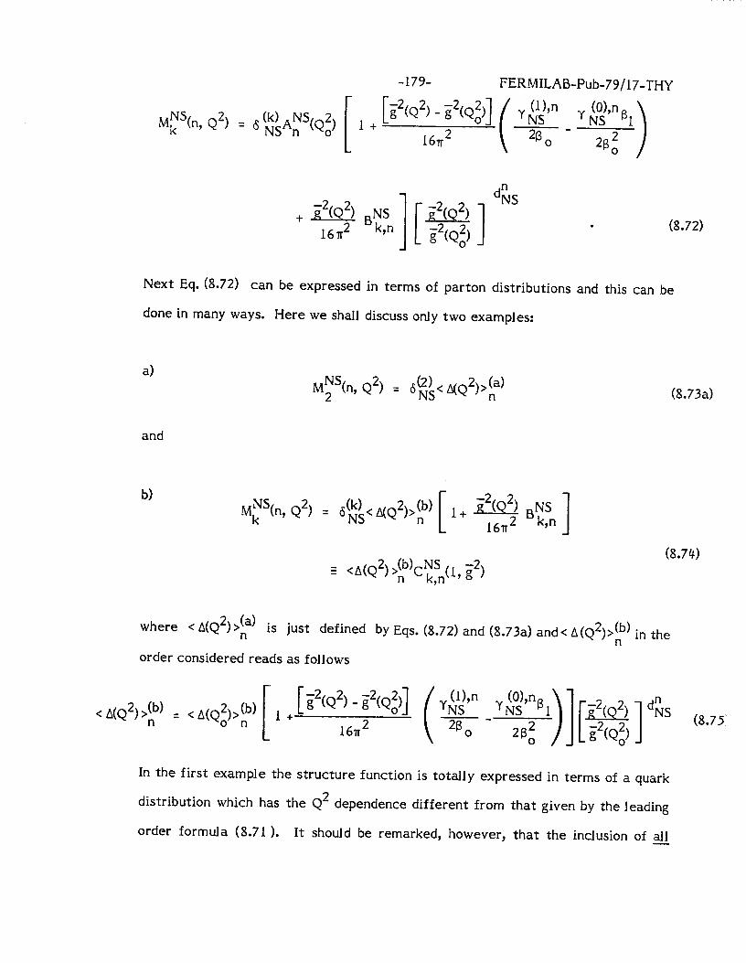
-179- FERMILAB-Pub-79/17-THY
+ E2(Q2) NS d”NS
16~’ Bk,n I[ 1 ii2(Q2)
i2(Q;) . (8.72)
Next Eq. (8.72) can be expressed in terms of parton distributions and this can be
done in many ways. Here we shall discuss only two examples:
a) and
b)
MyS(n, Q2) = 6::~ A(q2)>F)
MNS(n Q2) = k ’
-2( 2, NS l+-Bkn 161~~ ’ I
G <A(Q2) >(bt+ n k,-,(l, i+i2)
(8.73a)
(8.74)
where < A(Q2)>(a) . is n just defined by Eqs. (8.72) and (8.73a) and< a(~~)>:) in the
order considered reads as follows
< A(Q2) >(b) = < A(Q2)>(b) 1 + [ g2(Q2) - i2(Q;)]
n 0 n 161~~ (%$ -‘y;$+)][&&] d’s (8.75’
In the first example the structure function is totally expressed in terms of a quark
distribution which has the Q” dependence different from that given by the leading
order formula (8.71 ). It should be remarked, however, that the inclusion of all -
-180- FERMILAB-Pub-79/17-THY
higher order corrections into the definition of parton distributions can only be done
for one structure function, e.g. F2 as in Eq. (8.73a). The reason is that the parameters Bk n ,
depend on the structure function considered, and if the parton distribution is defined by
using F2, the formulae for the remaining structure functions (Fl, F3) will involve
explicit higher order corrections in addition to the parton distributions in question.
In the second example the term which depends on the structure function has
been factored out. Writing Eq. (8.74 ) as
MF’(n, Q2) = < A(Q2)>no tFn(Q2)
and using the convolution theorem of Eqs. (5.14-5.16) we obtain
F;%, Q2) = j- 1
X dy o rs( ; , Q2)A(b)(y, Q2)
(8.76)
(8.77)
The factor ok NS(x, Q2) can be interpreted as an elementary cross-section for
scattering of a current off a quark with an effective Q2 dependent distribution
A b) (y, Q2). This interpretation can be extended to other processes such as Drell-Yan,
large pl processes, etc., with o different for different processes. Therefore in this
formulation all measurable cross-sections are expressed as a convolution of
universal quark distributions and process dependent (also structure function
dependent) elementary parton cross-sections. This picture is at the basis of the
perturbative QCD to be discussed briefly in Section IX. It should be remarked,
however, that the parton distributions and the elementary parton cross-sections
defined in this way are separately renormalization-prescription dependent and
generally gauge dependent. These renormalization prescription and gauge
dependences cancel in the final expression if the same gauge and renormalization
scheme are used in the calculations of A (b) 2 (x, Q ) and o(x, Q 2 ). Since one can define
-181- FERMILAB-Pub-79/17-THY
parton distributions in many ways anyhow, one should not worry about this
renormalization prescription dependence of parton distributions discussed here.
The only important thing is to define the parton distributions consistently in the
same renormalization scheme for all structure functions and all processes.
Equations (8.73a) and (8.74a) can be generalized to the singlet structure functions.
In the case of definition a) one has (Altarelli, Ellis, Martinelli, 1978; Floratos, Ross and
Sachrajda, 1979)
M$n, Q2) = 6 (‘)<C (Q2)> (a) d.J n (8.73b)
where <C (Q*) >(a) _ n has rather complicated dependence on Q*. Explicit expressions for
<C (Q2) ,(a) n can be found in (Floratos et al., 1979). Notice that in this example all
higher order corrections (including those from gluon distribution) have been absorbed in
the definition of the singlet quark distribution.
Here we shall discuss in detail only the singlet analog of Eq. (8.74)
(Baulieu and Kounnas, 1978; Kodaira and Uematsu, 1978; Ellis, Georgi, Machacek,
Politzer and Ross, 1979). For the discussion of the distributions of Eq. (8.73b) we
refer the reader to the papers by (Altarelli, Ellis and Martinelli, 1978) and
(Fl oratos, R oss and Sachrajda, 1979). Equation (8.75 ) is just the non-singlet
formula (2.137). In order to derive Eqs. (2.138) and (2.139) we proceed as follows.
Using Eqs. (8.29) and (8.2) we first obtain
M$n, Q2) = An(p2)E2
(8.78)
-181a- FERMILAB-Pub-79/17-THY
with An(p2) and &g, 9 defined by Eqs. (8.30) and (8.5)’ respectively. Next in
analogy with Eq. (8.74 ) the moments <C(Q2),, and <G(Q2) >n are defined as
follows (we drop the index b in what follows)
[dQ*) >,,, < G(Q~)> n I E Anr,,2)$(g, 3
and consequently using Eq. (8.3) for Q* = p2 we obtain
M$n, Q2) = <C (Q2)>nC:n(l, g2) + <c(Q2)>,C$ .(l, g2) . Y Y
(8.79)
(8.80)
-182- FERMILAB-Pub-79/17-THY
Notice that since $(g, 3 = 1 for Q2 = u2, the parton distributions defined by (8.79 )
are just the matrix elements of various local operators renormalized at u2 = Q*. It
is now a simple matter to obtain Eqs. (2.138) and (2.139). In order to use some of
the results of Section VIILB we write (putting u2 = QE) Eq. (8.79) as follows
[ dQ2) >n, <G(Q2) >J = [ <C (Q;b,, <G(Q;) >J b ;I-l&g, $J fr-’ (8.81)
and use
[ 1 d”
- ii2(Q2) i2(Q;)
0
X
-2( 2) h l* h 1 - RQ u- v2u
161~~ (8.82)
where the matrix ?‘̂ v,“u is given by Eqs. (8.14)-(8.18). Inserting ( 8.82) into (8.81)
and using Eqs. (4.30) and (4.31) for 6 and G-1 we are led to the formulae (2.138) and
(2.139) which d escribe the Q2 evolution of <C (Q2) >n and <G(Q2)>,. Numerical
values of the parameters which enter these formulae are collected for the MS
scheme of Section VII in Table 2. In addition, g*/16 ~1~ 6 0 .03 for Q2 J‘ 5 GeV* and
therefore the next-to-leading order corrections in Eqs. (2.138) and (2.139) are
relatively small. Consequently the QL evolution of the parton distributions defined
by Eq. (8.79)’ with g2 corrections calculated in the m scheme, should not be very
different from the Q2 dependence predicted by the leading order expression of
-183- FERMILAB-Pub-79/17-THY
Section V. It would be interesting in the future to invert Eqs. (2.138) and (2.139) to G
obtain G(x, Q2) and X(x, Q2). The large value of the parameter K -+ for n = 4 and
f = 4 is related to the previously discussed singularity at dy = d_” + 1 which appears
for f z 3.8. The singularity in K G -+ is, however, cancelled by the factor multiplying
KG+ in Eq. (2.141)’ and the resulting correction is small. We would like also to remark
that due to properties (5.38)’ (5.39) and (X.42)’ Eqs. (2.138) and (2.139) satisfy energy
momentum conservation.
Al though the QL dependence of the quark and gluon distributions defined in
the MS scheme does not differ very much from the leading order predictions, the
input distributions for quark and gluon distributions which have to be taken from
the data will differ considerably at low Q* and large x from those used in the
-4J leading order phenomenology. The reason is that the parameters E;Sn and B2 n are Y Y
large for large values of n.
Finally as in the case of the non-singlet structure functions we can invert Eq.
(8.80) to obtain
F; (” Q*) = i ' dY [o;(; , Q2)x(y, Q2) + u ;(; , Q2)G(y, Q2) X 1 (8.83)
where o$(G, Q2) is, except for the charge factor, equal to o ys$ , Q2), and
o ;(; , Q2) can be interpreted as elementary cross-section for scattering of a
current (y, W, 2) off a gluon with an effective Q2-dependent distribution G(y, Q2).
So far nobody has done a detailed comparison of the higher order corrections
to the singlet structure functions with the experimental data but such a comparison
will be available in the near future (Field and Ross, 1979; Duke and Roberts,
1979b). F41 Some applications of these definitions of the parton distributions (Eqs. 8.73a, b,
8.74 and 8.80) in semi-inclusive processes are discussed by Altarelli et al. (1979b) and
Buras (1979).
F. More About Callan-Gross Relation
In this section we shall express the longitudinal structure function FL(x, Q2)
in terms of quark and gluon distributions. Combining Eqs. (7.18a) and (8.41) and
-184- FERMILAB-Pub-79/17-THY
utilizing Zq. (4.43) we first obtain the following expression for the moments of
FL(x, Q2)
ML(n, Q2) = Mp’(n, Q2) + M$n, Q2)
= GksA;S(Q;)
where
+ 6;A;tQ;) BL,n 2
8,JnQ A2
+(-A;(Q~) BL,n
f3,ln QZ A2
lnQf A2 [ I Q2
In o A2
-d:
[ lnQ1.
A2 Q2 In s2
A 1 -d;
Bin = Btn+ BG Y Y Ln
9 and BL G Y n and B L
Y n are given by Eqs. (2.98) and (2.1201, respectively.
Inserting Eq. (8.85 ) into (8.84 ) and using Eqs. (5.29-5.32) we obtain
ML(n, Q2) =
4J BL,n
B,lnd A2
M2(n, Q2) + BG
Lyn 2 B,InQ
A2
(8.84)
(8.85)
(8.86)
-185- FERMILAB-Pub-79/17-THY
where the Q2 dependence of M2(n, Q2) and of < G(Q2),, is given in the order
considered by the leading order formulae of Sections IV and V. As the reader may
convince himself Eq. (8.86) can also be derived from Eqs. ( 8.77) and (8.83 ) by
replacing there the indices k or 2 by the index L.
Finally using the convolution theorem of Eqs.
expressions for JI G bL n and B L n, as given in Eqs. (7.431, Y Y
(5.14)-(5.16) and the explicit
(8.56) and (8.571, we obtain
-7 FL(x, Q2) = ’ 2 j- ‘CiJ x2
8olne ’ y -q 9 F2(y, Q2) + d (218f(l
9 - ;)Y G(y, QL)J (8.87)
A2
In the case of four flavors &i2) = 6 for ep scattering and 6:’ = 1 for v 7 scattering Y .
Equation ( 8.87) with 6 (2) 5
60) = 9
= 18 agrees with Eq. (127) of (Al tarelli, 19781, and for
8 1 with Eq. (24) of (Kodaira and Uematsu, 1978) if we take into account that
the definition of FL(x, Q2) in the latter paper differs from our definition by a
factor x.
It should be emphasized that the parameter A which enters Eq. (8.87) need
not be the same as that obtained from the phenomenological applications of the
leading order or next-to-leading order expressions for the Q’ evolution of the
structure functions Fl, 2 F and F3 which do not vanish in the leading order. In fact
the value of A in Eq. (8.87) cannot be meaningfully determined from experiment un-
less 1/(1n2 Q2/A2) corrections to FL are computed. Therefore in comparing ( 8.87 )
with experiment we are free to choose A to be different from that extracted from
phenomenological applications of asymptotic freedom equations for other structure
functions. We do not think this point was realized previously in the literature.
-186- FERMILAB-Pub-79/17-THY
Experimentally the formula (8.87) is consistent with the ep data (Riordan et
al., 1975) for x < 0.4 (Hinchliffe and Llewellyn-Smith, 1977a) but disagrees with
these data for I arge x (De Rujula et al., 1977a). The predictions of the theory for
large x lie systematically below the data. This is also confirmed by the recent
analyses (Bodek et al., 1979 and Mestayer, 1978). The disagreement between
theoretical predictions and the data for FL might not be a problem for QCD,
however, and could be due to our neglect of higher twist F42 operators, non-
perturbative effects, etc., which are present in QCD but are difficult to calculate.
In particular it has been suggested by (Schmidt and Blankenbecler, 1977) that the
diquark systems in the proton could be responsible for the observed large values of
FL at large x. Recent phenomenological applications of this idea can be found in the
paper by (Abbott, Berger, Blankenbecler and Kane, 1979). Certainly the longitudinal
structure functions deserve further study.
-187- FERMILAB-Pub-79/17-THY
IX. ASYMPTOTIC FREEDOM BEYOND DEEP-INELASTIC SCATTERING
A. Preliminaries
So far our discussion of asymptotic freedom effects concentrated on deep-
inelastic scattering. In the past year there has been a lot of progress in
understanding the structure of asymptotic freedom in other than deep-inelastic
processes. For completeness we shall briefly review here some of the results of
these studies. We shall only discuss basic ideas and present results of various
calculations without confronting them with the data.
Historically, the study of asymptotic freedom in the inclusive deep-inelastic
scattering began in the framework of the formal approach of Section IV and only in
the last two years have calculations been made in the intuitive approach of Section
V and, in particular, in the framework of so-called perturbative QCD, which we
have not discussed so far. In the case of semi-inclusive processes, as for instance
massive u-pair production, or processes in which hadron momenta are measured in
the final state, progress proceeded in the reverse order. Most of the calculations
were first done in the framework of perturbative QCD and only recently have
studies been made to develop a technique similar to the powerful methods of
operator product expansion and renormalization group equations.
As we discussed in detail in this review, the operator product expansion (OPE)
allows us to identify systematically the dominant contributions to the moments of
the structure functions at large Q2 and to express them in terms of a sum of
products of (perturbatively) calculable coefficient functions and (by present
methods) incalculable matrix elements of certain operators taken between
hadronic states. The Q2 dependence of the coefficient functions can then be found
by means of renormalization group equations. In other words the OPE assures the
factorization of non-perturbative pieces (matrix elements of local operators) from
-188- FERMILAB-Pub-79/17-THY
perturbatively calculable pieces (coefficient functions). We would like to stress
that this factorization is true to all orders in the renormalized coupling constant gL
and in all logarithms of Q’ (leading, next-to-the leading, etc.). Such a proof has
been missing for semi-inclusive processes and the strategy (Politzer, 1977a, b;
Sachrajda, 1978a, b) has been to calculate these processes in perturbation theory in
g2 and to show that the non-perturbative pieces (mass singularities) can be factored
out and absorbed in the (by present methods) uncalculable wavefunctions of the
incoming and the outgoing hadrons. There have been very many papers on this
subject, and it is impossible to quote all of them here. An incomplete list of
theoretical papers involved with the question of factorization includes the works by
(Politzer, 1977a, b; Sachrajda, 1978a, b; Dokshitser, Dyaknov and Troyan, 1978;
Llewellyn-Smith, 1978b; Mueller, 1974, 1978; Libby and Sterman, 1978; Kazama and
Yao, 1978’1979; Amati, Petronzio and Veneziano, 1978a, b; Ellis, Georgi, Machacek,
Politzer and Ross, 1978a, 1979; Gupta and Mueller, 1979; Kripfganz, 1979; Frazer and
Gunion, 1979a, b). References to phenomenol ogical studies of semi-inclusive
processes can be found for instance in the reviews by (Field, 1979; Hwa, 1978;
Berger, 1979; Halzen, 1979).
In the theoretical papers above one can find demonstrations of all order
proofs of factorization (Ellis, et al., 1978a, 1979; Amati, et al., 1978a, b; Libby and
Sterman, 1978; Mueller, 1978) and a formulation of the whole study of semi-
inclusive processes similar to the formal approach of Section IV (Gupta and
Mueller, 1979).
Before we proceed with our review let us illustrate the idea of factorization
in the framework of perturbative QCD with the example of deep-inelastic
scattering (Politzer, 1977a).
-189- FERMILAB-Pub-79/17-THY
B. Factorization and Perturbative QCD
We consider the diagrams of Fig. 36 contributing to the photon-quark 2 F43 scattering to order g , and as in the calculations of Section VII we take the
incoming (massless) quarks slightly off-shell (p2 < 0). The result is most simply
expressed in terms of moments in x (Bjorken variable), and we obtain
i9.1)
where AZ stands for the empty (“bare”) blob in Fig. 36 and, as in Eq. (7.271,
r = T;Z,)PNS . n 9 The result (9.1) is not very useful for various reasons:
i) it is singular for p2-+ 0;
ii) the constants r n depend on our assumptions about the target, i.e., the 3
incoming quark. We could, for instance, perform the calculation with pL = 0 but
keep the quark mass m f 0. In that case we would obtain
(9.2)
where Fn f rn. In general rn or Fn are also gauge dependent. This is exactly the
same problem which we discussed in Section VIII, but we mention it here again
because it also enters the calculations of Drell-Yan and other semi-inclusive
processes as we shall see below. Of course we know already how this problem is
solved (see Section VIII), and we shall leave it for a moment.
The problem i) is solved by first rewriting Eq. (9.1) as follows (we drop
constant terms)
FERMILAB-Pub-79 /17-THY
0 Mn = A; l+~yNslnZZ
16~r~ 2 P2 I (9.3)
and then absorbing the p2 dependent singular factor into A”,. We obtain therefore
%n Mn q An(u2) l-g- 2 ‘NS ln $
16.rr2 2 v2 (9.4)
where u is an arbitrary scale which we introduced to protect the Q2 dependent
factor from the singularity at p2 = 0.
In the parton language we can interpret An(u2) as the moments of a parton
distribution at Q2 = u2. In the formal language this is just the matrix element of
Eq. (7.29). The second factor on the r.h.s. of Eq. (9.4) describes how the moments
Mn behave for Q2 f u2. Notice that this factor is free of any singularity for p2 + 0.
In formal terms it is just the coefficient function calculated to first order in g2
(keeping only the leading logarithm). This factorization of singular (non-
perturbative) terms from well-behaved terms can be proven to all orders in
perturbation theory in g2 (see references above). When all orders in g2 are summed
and in each order only leading logarithms are kept, then the leading order
corrections of asymptotic freedom discussed in the previous sections are obtained.
Summing next-to-leading logarithms to all orders in g2, one obtains the next-to-
leading order corrections of asymptotic freedom of Sections VII and VIII, and so on.
C. Lessons from Deep-Inelastic Scattering
In our presentation of asymptotic freedom effects in processes other than
deep-inelastic scattering we shall discuss both the leading and next-to-leading
order corrections, and it is useful to summarize the lessons which we gained from
the study of deep-inelastic scattering. They are as follows:
, -191- FERhULAB-Pub-79/17-THY .
a) In the leading order there is no reason that the numerical values of the
scale parameter A should be the same for different processes.
b) If next-to-leading order effects are taken into account and the effective
coupling constant defined universally for various processes,then it is justified to use
the same value of A in different processes (here we tacitly assume that still higher
order corrections Q&(Q2)) are small).
c) The definition of parton distributions is not unambiguous beyond the
leading order. Therefore in comparing the parton distributions extracted from
various processes one has to make sure that the definition of parton distributions is
common to all processes.
d) dne has to make sure that all renormalization prescription-dependent parts
of a physical expression are calculated in the same scheme, so that at the end a
renormalization prescription-independent answer is obtained
e) One has to check that the final answer for the coefficient functions does
not depend on the (in principle arbitrary) assumptions about the gluon and quark
target us&d in perturbative calculations to extract the coefficient functions.
We shall keep these lessons in mind while discussing various processes. We
begin our presentation with e’e- annihilation.
D. e+c’ + hadrons
This process has been studied in the framework of asymptotically free gauge
theories already a long time ago (Appelquist and Georgi, 1973; Zee, 1973).
Therefore we only quote the result and discuss it briefly.
Consider the ratio
(9.5) . R- o(e+e- + hadrons) g(e+e- + lJ+lJ
-192- FERMILAB-Pub-79/17-THY
In the simple parton model and in QCD one obtains for Q2 : E: m+ oo . .
Ra = 3 1 ei2 i
(9.6)
where 3 is the number of colors, ei are the charges of the quarks and the sum runs
over the flavors. The fact that R approaches a constant value is a consequence of
the lack of renormalization of the conserved electromagnetic current. For finite
values of Q2 there are calculable asymptotic freedom corrections to Eq. (9.6), and
the formula for R reads as follows
R = R= C
1 + i2(Q2) b + ii%& b + . . . 16?t2 ’ (16n2)2 2 1 . (9.7)
The coefficient bl has been calculated by (Jost and Luttinger, 1950; Appelquist and
Georgi, 1973; Zee, 1973) and is given as follows
bl = 4 . (9.8)
Neglecting for the moment 2(Q2) corrections and using the leading order
-2 2 expression for g (Q ) (Eq. 2.50) one obtains
(9.9)
bl is positive and, therefore, R, will be approached from above. In Fig. 37 R is
plotted as a function of f- Q2 for f = 4 and -~two values of A. The contribution of
the heavy lepton (AR = 1) have been added there. The experimental values of R range
at Q2- r - 5 GeV from 4.5 to 5.0 (see review by Feldman, 1979). The CI~TVSS in Fig. 37
-193- FERMILAB-Pub-79/17-THY
are shown only to illustrate the size of the second term in Eq. (9.9). A careful corn-
parison of Eq. (9.9) with the data involves smearing over the resonances and inclusion
of threshold effects. We refer the interested reader to the papers by (Poggio, Quinn
and Weinberg, 1976; Moorhouse, Pennington and Ross, 1977; Barbieri and Gatto, 1977;
Shankar, 1977) for details. Recalling lesson a) there is no reason why the value for
A extracted from the data on the basis of Eq. (9.9) should be the same as that
obtained from the leading order analysis of deep-inelastic scattering. A meaningful
comparison of QCD effects in e+e- annihilation with those expected in deep-
inelastic scattering can, therefore, only be made once the 2 corrections are taken -2 2 into account as in Eq. (9.7). Using Eq. (2.88) for g (Q ) calculated to two loops, we
obtain from (9.7)
R =R co bl
@,ln$ A2
2
81 In In Q-
A2 “‘2 -
0 In’@ A2
L +
i3: ln2 Q! A2
+ . . . I . (9.10)
Of course the exact value for b2 in the expansion in Eq. (9.10) depends on the
definition of g2(Q2) or, equivalently, on the definition of A. Resealing A to A’ with
A = KA’ (9.11)
changes the last term in Eq. (9.10) to
b2 +Bobl In K’
(9.12)
-194- FERMILAB-Pub-79/17-THY
with A replaced by fl’ in the first two terms. The calculation of b2has been recently done
by (Dine and Sapirstein, 1979; Ross, Terrano and Wolfram, 1979; Celemaster and Gonsalves,
1979) with the result b2 = 89.3, 24.3, -27.2 for h4S, !% and MOM schemes, respectively.
Since i2/16n2 is 0 (0.03) for Q2 z 30 GeV2 we observe that 2 corrections to R are
relatively small.
E. Photon-Photon Collisions
It is well-known that photon-photon inelastic collisions in e+e- storage rings
become an increasingly important source of hadrons as the center-of-mass energy
is raised (Brodsky, Kinoshita and Terazawa, 1971; Terazawa, 1973; Budnev et al.,
1975). Whereas the e+e- annihilation cross-section decreases quadratically with
energy, the cross-section for e+e- + e+e- + hadrons increases logarithmically with
energy. The dominant contribution to the latter cross-section arises from the
annihilation of two nearly on-shell photons emitted at small angles to the beam.
Here we shall study the case in which one of the virtual photons is very far off-
shell (large Q2) and the other one is close to the mass shell (small p2) as shown in
Fig. 38.
The subprccess
Y +Y -f hadrons (9.13)
can be viewed as deep-inelastic scattering on a photon target. The corresponding
virtualCompton amplitude is shown in Fig.38b,and as in the standard deep-inelastic ..,
scattering one can introduce structure functions as Fi, this time photon structure
functions. In the early days process (9.13) was studied in the framework of the
Vector Dominance Model (VDM) and predictions similar to that for standard deep-
inelastic scattering have been obtained, i.e., Bjorken scaling in the simple parton
model and logarithmic scaling violations in the framework of asymptotically free
gauge theories (Ahmed and Ross, 1975a). It turns out, however, that in addition to
the VDM contributions there are contributions to photon-photon scattering in which
the photon behaves as a point-like particle (Walsh and Zerwas, 1973; Kingsley,
1973). In the parton model these contributions are represented by the box diagram
-195- FERMILAB-Pub-79/17-THY
of Fig. 38~. The box diagram contribution can not only be exactly calculated, but at
large values of Q2 increases as In Q2 and dominates over the (incalculable in
perturbation theory) vector dominance terms. The latter are suppressed by powers
of In Q2 as in the standard deep-inelastic scattering. Neglecting VDM contribu-
tions, the parton model result for the photon structure function F:(x, Q2) for large
Q2 has the form
F;(x, 4’) 1 PM = 2 2P(Xh Q2 (9.14)
where a is the electromagnetic coupling constant and p(x) is given as follows
p(x) = 8 6y xPqG(x) (9.15)
Here P ,,(x) is the familiar splitting function of Eq. (2.57) which expresses the
probability of finding a quark in a gluon (now photon). Furthermore
6 31 4 y= iei (9.16)
where the sum runs over the flavors and ei are the quark charges. “3” stands for
the number of colors.
It has been pointed out by (Witten, 1977) that there are asymptotic freedom
corrections to the parton model result of Eqs. (9.14) and(9.15). Witten calculated
these corrections in the leading order of asymptotic freedom and his calculation
has recently been extended to the next-to-leading order (Bardeen and Buras,
1979a). All these corrections are independent of the unknown matrix elements of
local operators in contrast to the case of standard deep-inelastic scattering, and
can be exactly calculated. Moreover, at sufficiently large values of Q2 these
exactly calculable ter,ms are more important than the VDM contributions.
-1% FERMILAB-Pub-79/17-THY
Therefore the process under consideration is, from a theoretical point of view, an
excellent place to study properties of higher order corrections. The two
calculations above have been done using operator product expansion and renormali-
zation group methods. Witten’s result has been rederived last year by Llewellyn-
Smith (1978~) and recently by (Frazer and Gunion, 1979) in the framework of
perturbative QCD. Furthermore, the process in question has been studied in the
intuitive approach of Section V (De Witt, Jones, Sullivan, Willen and Wyld, 1979;
Brodsky, De Grand, Gunion and Weis, 1978, 1979P4!n what follows we shall present
in more detail the formal approach to photon-photon scattering.
The formal approach to photon-photon scattering has been first discussed by
(Witten, 1977). The moments of the photon structure function Fl(x, Q2) are given
as follows
s1 0
dx x”-‘F;(x, Q2) = 1 C; n i 9
g2 , g2, IJ
(9.17)
where c1 = e2/4n is the electromagnetic coupling constant. The sum on the r.h.s.
of Eq. (9.16) runs over spin n, twist 2 operators such as the fermion non-singlet
operator ONs, singlet fermion and gluon operators, 0 4)
and OG, and the photon
operator 0 y. The latter operator which is not present in the analysis of the deep-
inelastic scattering off hadronic targets, is the analog of the gluon operator OG
with the non-abelian field strength tensor G aB replaced by the electromagnetic
tensor F ClB (see Eq. (3.57)). As noted by Witten, Oy must be included in the
analysis of photon-photon scattering. The reason is that, al though the Wilson
coefficients Ci are O(a), the matrix elements <y ) 0” 1 y> are O(1). Therefore the Y
photon contribution in Eq. (9.17) is of the same order in a as the contributions of
quark and gluon operators. The latter have Wilson coefficients O(1) but matrix
elements in photon states O(a). We want to evaluate Eq. (9.17) to lowest order in o
but to all order in g. In lowest order in ~1
-197- FERMILAB-Pub-79/17-THY
i = +,G,NS
where the functions on the r.h.s. of Eq. (9.18) are the familiar Wilson coefficients
which we discussed in Sections II-VIII. (Recall that the coefficient functions do not
depend on the target.) Therefore the first three terms involving hadronic operators
will be suppressed by powers of logarithms except for n = 2 due to the vanishing of
the anomalous dimension of the hadronic energy momentum tensor. Moreover, the
matrix elements of hadronic operators in photon states cannot be calculated in
perturbation theory. In the language used above the three terms in Eq. (9.17)
involving hadronic operators belong to Vector Dominance contributions. We are, in
fact, mainly interested in the coefficient function of the photon operator, whose
matrix element between photon states is known,
(9.18)
<yIoylY’ = 1 .
C:,n(Q2/u2, g2, ~1) satisfy the following renormalization group equations
(9.19)
a l$i
Qf 2 29g ,a i = + ,NS,G,y (9.20) 1-1
where y.. 11
are the elements of the 4 x 4 anomalous dimension matrix which has in
lowest order in c1 the following structure
(9.21)
-198- FERMILAB-Pub-79/17-THY
Here Tr(g’) is the standard hadronic anomalous dimension matrix of Eq. (4.22)
extended by one column and one row to include the anomalous dimension of the
non-singlet operator. -f Kn(g2, a) is a three component vector
kn(g2, 03 = n 2 K,$g 7 a), K;(g’, a), Kis(g2, ~1) 1 which represents the mixing between the photon operator and the remaining three
operators. The components Kn 1
can be calculated in perturbation theory and have
the following expansion
e2 K;(g’, a) = - - K&n .‘g2 K(l)$ 16~? j 2 j
j = $,NS
(167r’) (9.23)
(9.22)
and
K;(g2, a) = _ 4 Kt)‘” (9.24) (16~~)
Examples of diagrams necessary for the calculation of the coefficients Kppn, (l),n K.
and Kt)yn I I
are shown in Fig. 39.
Because of the mixing between the photon operators and hadronic operators
the coefficient function Cg,n(Q2/u2, g2, a) depends on the matrix qt(g’) and the
coefficients ?$,(I, g2), Cyfn(l, 8’) and C!$n(l, g2), in addition to the mixing
anomalous dimensions K)and the coefficient function C $,,(l, g2, a). The resulting
expression for the moments of F:(x, Q2) is as follows
dx x”-‘F;(x, Q2) = a2 an In 2 0 I2
+ “an In In (9.25)
where the terms O(l/(ln Q2/x2)) include the VDM contributions.
-199- FERMILAB-Pub-79/17-THY
The constants an have been calculated by (Witten, 1977) and the parameters
gr, and bn by (Bardeen and Buras, 1979a). The a, depend on one-loop anomalous
dimensions and one loop B functions while the zn depend, in addition, on the two-
loop contributions to the B functions. Finally, the En depend on the two-loop
anomalous dimensions and the one-loop contributions to the Wilson coefficient
functions, in addition to the renormalization group parameters on which “an and an
depend. Analytic expressions for an, “a,., and En and their detailed derivations can
be found in the original papers. The numerical values for these parameters are
collected in Table V. The numerical values of E,.., depend on the definitions of the
scale parameter X. The Kn in Table V are for the= of Section VII. Notice that
we do not give the values of b2, which involves the perturbatively uncalculable
photon matrix element of the hadronic energy momentum tensor.
Remembering lesson b) of Section C we take for x the value of 0.5 GeV which
we have extracted from deep-inelastic scattering in Section VII using the same __.
definition for A. Equation (9.25) is plotted in Fig. 40 for various values of n on Q2.
In Fig. 40 L.O. stands for the first term in Eq. (9.26) and PM stands for the parton
model result of Eq. (9.15). We conclude that asymptotic freedom effects suppress
the photon-structure function at large values of n or equivalently large x and that
this suppression is enhanced by higher order corrections as compared to the leading
order result. A similar result for the higher order corrections to the moments of
Fz(x, Q2) is obtained if g2(Q2) is defined by momentum subtraction. In that case
the parameters b,, are replaced (Celemaster and Gonsalves, 1979) by
brnorn = 6 n n + a,[ 1.541 (9.26)
-2oo- FERMILAB-Pub-79/17-THY
and x = 0.5 GeV by Amom = 0.85 GeV as extracted in this scheme from deep-
inelastic scattering (see Section VI1.I-I). More elaborate comparison of higher order
corrections with the I eading order result and the higher order corrections in deep-
inleastic scattering can be found in the paper by (Bardeen and Buras, 1979a).
For recent reviews of the photon-photon physics in connection with QCD
ideas we refer the interested reader to the papers by (Llewellyn-Smith, 1978c;
Brodsky, et al., 1978; Brodsky, 1978; Kajantie, 1979; Koller, Walsh and Zerwas,
1979; Hill and Ross, 1979). In particular Hill and Ross discuss heavy quark mass
effects in photon-photon scattering which turn out to be important.
F. Semi-inclusive Processes in QCD
1. Preliminaries
We shall now turn to the presentation of the basic structure of QCD formulae
for semi-inclusive processes. To this end it will be useful to introduce certain
notation which we shall illustrate with the familiar deep-inelastic scattering.
Consider a photon of momentum q which scatters off a parton of momentum p. If
P is the momentum of the hadron to which the parton in question belongs then we
can introduce the following variables
d- x = 2P.q
Z=& .
and 5, the fraction of the hadron momentum carried by the struck parton.
(9.27)
(9.28)
The deep-inelastic photon-hadron cross-section can then be written in QCD as
-2Ol- FERMILAB-Pub-79/17-THY
u H(x, Q2) = 1 J dx”JdS&(x j
- “XS )u~(~, Q2) ’ 5 fr(S, Q2) 1
= c il j x
‘+ 0 ;f, Q2) [ 5 f;( 5, 4') 1 . (9.23)
Here o j P
is the photon-parton cross-section and f .H * I
IS the distribution of partons of
type j in the hadron. The sum runs over all types of partons, i.e. quarks and gluons.
Eq. (9.29) just represents Eqs. (8.77) and (8.83). Eq. (9.29) is illustrated in Fig. 41.
In the leading order of asymptotic freedom
u;(x, Q2) = I .fs (1 - “x) j =a5
(3.30) 1 0 j=G
and
4 fp(S, Q2) f Sqj(s, 4’) or SClj(s 3 4’) (9.31)
with Q2 dependence given by Eqs. (2.52-2.54). Inserting Eqs. (9.30) and (9.31) into
(9.29) we obtain the standard result
oH(x, Q2) = 1 e? [ Xqj(X, Q2) + X4j(X, Q2)l j ’
. (9.32)
which is also true in the simple parton model if QL is neglected. If next-to-the-
leading order corrections are taken into account the following things happen
i) there are g2(Q2) corrections to the photon-quark cross-sections of Eq.
(9.30);
-202- FERMILAB-Pub-79/17-THY
ii) the Q2 dependence of quark distributions is modified (see Eqs. 2.137-2.139);
iii) the photon-gluon cross-section, which is of order g2(Q2), also enters the
final formula for aH(x, 4’).
As discussed extensively in Section VIII the points i)-iii) are related to each other.
For instance the explicit g2(Q2) corrections to various parton cross-sections depend
on the definition of parton distributions beyond the leading order.
In what follows we shall briefly discuss QCD formulae for semi-inclusive
processes, which will turn out to have a structure similar to that of Eq. (9.29).
2. Fragmentation functions
In addition to quark distributions, extensively discussed in previous sections,
important quantities in the study of semi-inclusive processes are the fragmentation
functions (Feynman, 1972; Field and Feynman, 1977 ) which describe how a parton
decays into a final hadron. The best process (at least from a theoretical point of
view) to study these functions is the semi-inclusive e+e- annihilation in which a
single hadron is detected in the final state:
e+e- -t h(P) + anything
This process is shown in Fig. 42.
The relevant variables are, in analogy with Eqs. (9.27) and (9.28),
(9.33)
(9.34)
and
2 = 23is
Q2 (9.35)
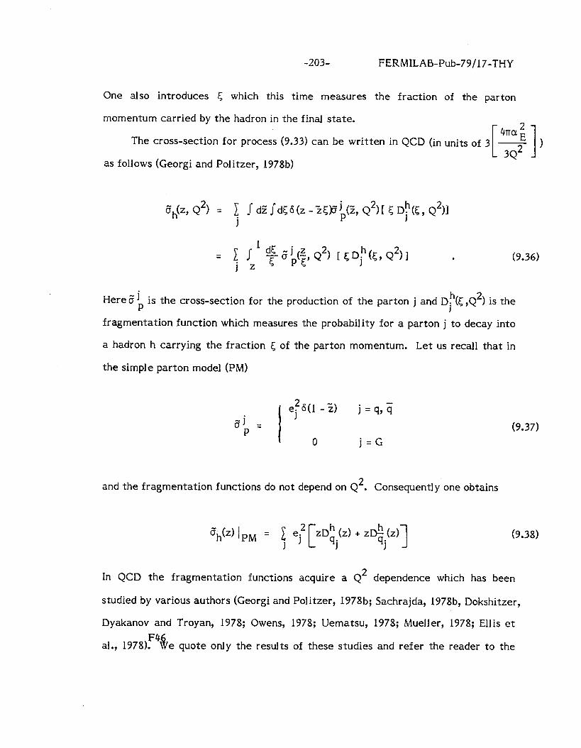
-203- FERMILAB-Pub-79/17-THY
One also introduces 5 which this time measures the fraction of the parton
momentum carried by the hadron in the final state. 4lTo;
The cross-section for process (9.33) can be written in QCD (in units of 3 - [ 1 34’ 1
as follows (Georgi and Politzer, 1978b)
’ dE -j(= Q2) C $(5, Q2)1 -pP~’ . (9.36)
HereGj * p IS the cross-section for the production of the parton j and D:(c ,Q2) is the
fragmentation function which measures the probability for a parton j to decay into
a hadron h carrying the fraction < of the parton momentum. Let us recall that in
the simple parton model (PM)
I
j=q,i ,j =
P 0 j=G
and the fragmentation functions do not depend on Q2. Consequently one obtains
a”$d /PM = zDh (z) + z& (z) qj 4j 3
(9.37)
(9.38)
In QCD the fragmentation functions acquire a QL dependence which has been
studied by various authors (Georgi and Politzer, 1978b; Sachrajda, 197833, Dokshitzer,
Dyakanov and Troyan, 1978; Owens, 1978; Uematsu, 1978; Mueller, 1978; Ellis et
al., 1978)r4&e quote only the results of these studies and refer the reader to the
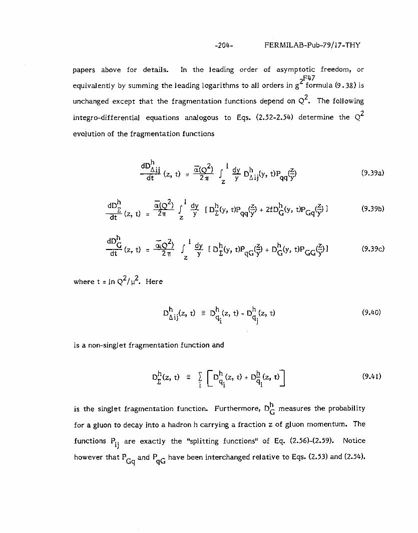
-204- FERMILAB-Pub-79/17-THY
papers above for details. In the leading order of asymptotic freedom, or
equivalently by summing the leading logarithms to all orders in g 2F47
formula (9.38) is
unchanged except that the fragmentation functions depend on Q2. The following
integro-differential equations analogous to Eqs. (2.52-2.54) determine the Q2
evolution of the fragmentation functions
dDh CL2 ld f [ D$y, t)Pqq(;) + 2f I&, t)PGq$j 3 dtC (z, t) = + i,
(9.39a)
(9.39b)
dDh $,z, t) = * l,i + [ D;(y, tPq& + D$y, t)P& 1 (9.39c)
where t = In Q2/ u2. Here
Diij(z, t) q D; (z, t) - Dh (z, t) i qj
(9.40)
is a non-singlet fragmentation function and
D,h(z, t) - “[
D; (z, t) + + (z, t) i i i 1 (9.41)
is the singlet fragmentation function. Furthermore, Dk measures the probability
for a gluon to decay into a hadron h carrying a fraction z of gluon momentum. The
functions Pij are exactly the “splitting functions” of Eq. (2.56)-(2.59). Notice
however that PCs and PqG have been interchanged relative to Eqs. (2.53) and (2.54).
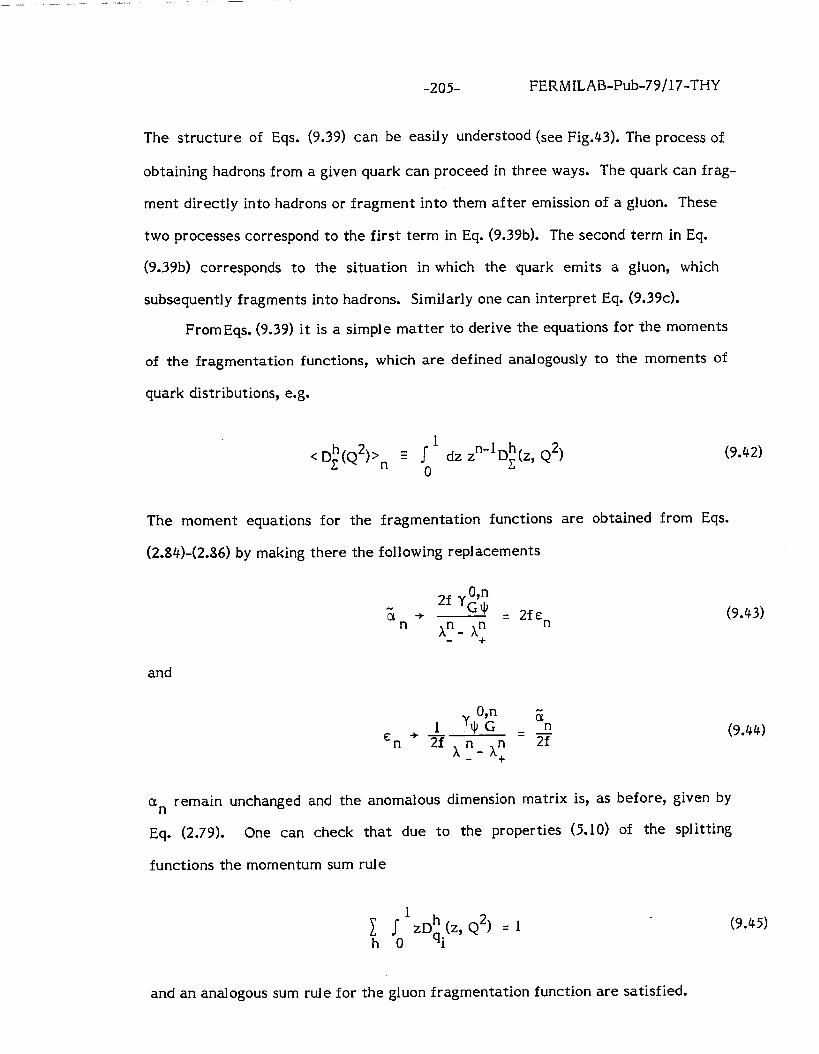
-205- FERMILAB-Pub-79/17-THY
The structure of Eqs. (9.39) can be easily understood (see Fig.43). The process of
obtaining hadrons from a given quark can proceed in three ways. The quark can frag-
ment directly into hadrons or fragment into them after emission of a gluon. These
two processes correspond to the first term in Eq. (9.39b). The second term in Eq.
(9.39b) corresponds to the situation in which the quark emits a gluon, which
subsequently fragments into hadrons. Similarly one can interpret Eq. (9.39~).
FromEqs. (9.39) it is a simple matter to derive the equations
of the fragmentation functions, which are defined analogously to
quark distributions, e.g.
1 < D;(Q2)>n = j- dz z”-‘D;(z, 4’)
0
for the moments
the moments of
(9.42)
The moment equations for the fragmentation functions are obtained from Eqs.
(2.84)-(2.86) by making there the following replacements
(9.43)
and
(9.44)
an remain unchanged and the anomalous dimension matrix is, as before, given by
Eq. (2.79). One can check that due to the properties (5.10) of the splitting
functions the momentum sum rule
1 1 j- zD; (z, 4’) = 1 h0 i
(9.45)
and an analogous sum rule for the gluon fragmentation function are satisfied.
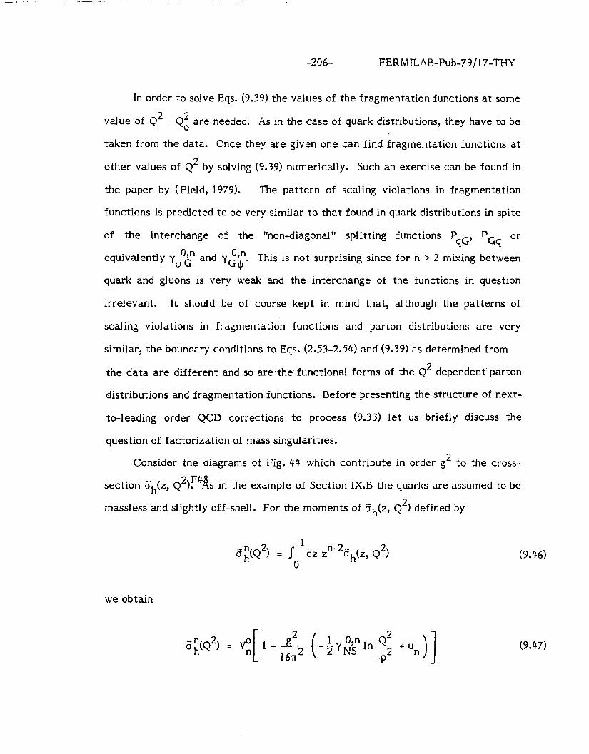
-206- FERMILAB-Pub-79/17-THY
In order to solve Eqs. (9.39) the values of the fragmentation functions at some
value of Q2 = Qz are needed. As in the case of quark distributions, they have to be
taken from the data. Once they are given one can find fragmentation functions at
other values of Q2 by solving (9.39) numerically. Such an exercise can be found in
the paper by (Field, 1979). The pattern of scaling violations in fragmentation
functions is predicted to be very similar to that found in quark distributions in spite
of the interchange of the “non-diagonal” splitting functions P w ‘Gq Or
equivalently y $2 and y$$. This is not surprising since for n > 2 mixing between
quark and gluons is very weak and the interchange of the functions in question
irrelevant. It should be of course kept in mind that, although the patterns of
scaling violations in fragmentation functions and parton distributions are very
similar, the boundary conditions to Eqs. (2.53-2.54) and (9.39) as determined from
the data are different and so arethe-functional forms of the Q2 dependent- parton
distributions and fragmentation functions. Before presenting the structure of next-
to-leading order QCD corrections to process (9.33) let us briefly discuss the
question of factorization of mass singularities.
Consider the diagrams of Fig. 44 which contribute in order gL to the cross-
section G,(z, Q2)F4w s in the example of Section 1X.B the quarks are assumed to be
massless and slightly off-shell. For the moments of Z,(z, Q2) defined by
Z,“(Q’, = j- 1
dzz 0
n-2:&, Q2)
we obtain
2 -$yl,$nln% + u
-P n )I
(9.46)
(9.47)
-207- FERMILAB-Pub-79/17-THY
where Vz stands for the empty (“bare”) blob in Fig. 44, yiin is the standard non-
singlet anomalous dimension and un are constant numbers analogous to the m’s of
Eq. (9.1). As in Eq. (9.1) also here there is a mass singularity for p2 + 0 and un
depends on the assumption about the quarks. For m2 f 0 and p2 = 0 a different un
would be obtained. Equation (9.47) can be rewritten as follows
+uf))] [ I+$(-$y$J*n$ +u~))] (9.48)
where u2 is a scale and
&I) + p = u . n n n (9.49)
Combining the first two factors on the r.h.s. of Eq. (9.48) we obtain
Zh(Q2) = V(u2) n n (9.50)
In the parton language we can interpret V,(p’) as the moments of the
fragmentation function at Q2 = u2. In the formal language of (Mueller, 1978),
Vn(u2) is an analogue of the matrix element of local operator and is called the
time-like cut vertex. In the same language the matrix elements of local operators
are called space-like cut vertices. The second factor on the r.h.s. of Eq. (9.50)
which is free of any singularity as p2 + 0 is the analogue of the coefficient
function. This time a coefficient function of the time-like cut vertex in an expansion
similar to the operator product expansion.
This factorization of singular (non-perturbative) terms from well behaved
terms which can be calculated in perturbation theory can be proven to all orders in
-20% FERMILAB-Pub-79/17-THY
g2 and in all logarithms (Ellis et al., 1978, 1979; Amati et al., 1978a, b; Mueller,
1978).
(2) (1) Notice that through Eq. (9.49) un depends on un or equivalently on the
normalization of the cut vertex at p2 = p2. Different renormalization schemes will
(2) therefore lead to different values of un . As in the case of deep-inelastic
scattering, also here this renormalization prescription dependence will be cancelled
by that of the two-loop anomalous dimensions of the cut vertices when the full Q2
evolution of the fragmentation function to all order in g2 and in the first two
orders in E2 is calculated. We observe, therefore, that the study of the next-to-
leading order corrections to the Q2 evolution of the fragmentation functions
proceeds in an analogous way to that for quark distributions. The structure of the
formal and intuitive formulae (beyond the leading order approximation) for the
process (9.33) is very similar to that presented in the previous sections for deep-
inelastic scattering. Questions of definitions of fragmentation functions, of the
definition of z2(Q2) and of the cancellation of renormalization-prescription
dependences also arise here. Consequently also the comments i)-iii) made after Eq.
(9.32) also apply toEn(z, 4’) as given in Eq. (9.36).
Eq. (9.50) can be rewritten as follows
L;; =<D(Q*)‘, 1 + “(2) g2 16~’ n 1
where
<D(Q*)>n = Vn(u2) ’ ‘NS O,n 2
1 - 5 7 lnQ2 161~ .’ P 1
(9.51)
(9.52)
are the moments of the fragmentation functions and
-209- FERMILAB-Pub-79 /17-THY
(9.53)
are the moments of the cross-section for quark production calculated to order g2.
When all orders in g2 -2 2 and the two first orders in g (Q ) are taken into account,
<D(Q’) >,., acquires the full Q2 dependence with two-loop anomalous dimensions of the
cut vertices and the two-loop B function included. Furthermore, in Eq. (9.53) g2 is
h . replaced by g2(Q2). We recall once more that, although Gn is unambiguous, the
Mh separation of a, into the fragmentation function and the cross-section for parton
production is arbitrary beyond the leading order. -2 2 The full study of g (Q ) corrections to the process e+e- + h + anything has not
yet been discussed in the literature. In particular, it is not known whether the two-
loop anomalous dimensions for time-like cut vertices are the same as those for
space-like cut vertices (I ocal operators).
3. Drell -Y an and semi-inclusive deep-inelastic scattering
In the simple parton model, parton distributions and parton fragmentation
functions are the building blocks of any expression for inclusive and semi-inclusive
processes. These building blocks do not depend on the process, although in
different processes they enter in different well-defined ways. Thus if we can
extract all parton distributions from deep-inelastic processes and fragmentation
functions from e+e- annihilation, then the cross-sections for other processes such
as the Drell-Yan process (Drell and Yan, 1971), semi-inclusive deep-inelastic scat-
tering, etc. can be predicted.
We have seen that, in QCD, parton distributions and fragmentation functions
acquire a Q2 dependence, and it is of interest to ask whether the QCD predictions
for semi-inclusive processes amount to using these Q2 dependent functions in the
-210- FERMILAB-Pub-79 /17-THY
parton model formulae for the processes in question. This has been studied by
many authors during the last year, in particular by (Politzer, 1977a; Sachrajda,
1978a, b; Dokshitser, Dyakanov and Troyan, 1978; Llewllyn-Smith, 1978b; Amati et
al., 1978a, b, c; Ellis, Georgi, Machacek, Politzer and Ross, 1978, 1979; Gupta and Mueller,
1979; Buras, 1979). In what follows we shall present the formulae for the two processes
eH + e + h + anything , (9.54)
and
HlH2 + u+u- + anything (9.55)
in the leading order and next-to-leading order of asymptotic freedom. Subse-
quently, we shall briefly discuss the basic features of these formulae which are
characteristic for all QCD expressions for semi-inclusive cross-sections.
The cross-sections for the processes (9.542 and (9.55) are given in QCD as
follows:
GHh(x, z, Q2) = 1 ./. d”zdx;lSldS+ (x - x”S,)&(z - tc,) j,k
z$(:, 2, Q2) $fjH($, Q2) 1 [ c2D;(5,, Q2)l
= ‘+ 1,l d%$‘k(~,<,Q2) [$fjH(S,, Q2) 11 52D;(5,, 4’) 1 (9.56)
for process (9.54) and
-21 l- FERMILAB-Pub-79/17-THY
do 4~; r dxl dx2 --
iq - J -4
34’ ‘1 x2 offH2(Xl’ 37 x129 Q2) (9.57)
with
~H~H~(x~, ~29 ~129 4’) = 7 j fi1G2d51d526(xl - “xl6 l)6(x2 - Z2<,) j,G
jkCx x” j; cJ p 1’ 2’ 12’ Q2)[ SlfjH1( 51, Q’)] [C 2fr2(C2, Q’)] (9.58)
= 1 j-l dA j- ’ dS2 obk ( z ,; ,$, Q2) [SlfJ?Cl, Q’)] [C2f;2(S2, Q2g j,k x1 51 x2 52 2
for process (9.55). In Eq. (9.57) oE is the electromagnetic coupling constant. The
processes are shown schematically in Figs. 45 and 46. Variables xi, “xi, 5 i in Eqs.
(9.57) and (9.58) are obvious generalizations of the variables of Eqs. (9.27) and
(9.28). The new variable xl2 is given as follows
2(Pl’ qXP2 - q) X 12 = Q’(P,. P,)
and Z12 is obtained from xl2 by replacing Pi by pi. Furthermore T = Q 2 /s, where
s = (P, + P,)2.
In Eq. (9.56) Gbk stands for the photon-parton j cross-section with the parton
k in the final state. The parton j belongs to the incoming hadron H and its
distribution is given by $fjH(cl, Q2) with 5 1 being the momentum fraction of H
carried by parton j. The parton k, on the other hand, fragments into the hadron h,
and this process is described by the fragmentation function C,D# 2, 4’). The
sums in Eq. (9.56) run over all types of partons i.e. quarks and gluons. Similar
-212- FERMILAB-Pub-79/17-THY
jk comments apply to Eq. (9.58) with u P being the cross-section for parton j-parton k
scattering or annihilation with a p+ p- pair in the final state.
Formulae (9.56) and (9.58) are obtained by summing various QCD diagrams to
all orders in g2. Keeping leading logarithms in each order corresponds to the
leading order in g2(Q2). Summing next-to-leading logarithms corresponds to next-
to-leading order in g2(Q2) and so on. As in deep-inelastic scattering and semi-
inclusive e+e- annihilation, one encounters mass singularities which must be
factored out and absorbed in the incalculable (in perturbation theory) wave
functions of the incoming and outgoing hadrons: parton distributions and
fragmentation functions or in more formal language space-like and time-like cut
vertices. The structure of mass singularities (anomalous dimensions) turns out to
be the same for incoming hadrons as in deep-inelastic scattering and for outgoing
hadrons as in e+e- annihilation. Therefore the parton distributions and parton
fragmentation functions be defined universally independent of the process
considered. We write ,lcan,l because, due to ambiguities in the definition of parton
distributions and parton fragmentation functions beyond the leading order of
asymptotic freedom, one could in principle define parton distributions in a different
way for different processes. This of course would not be a very useful thing to do.
Let us discuss Eqs. (9.56) and (9.58) in slightly more detail. In the leading
order of asymptotic freedom
oP - jk(;;, 2, Q2) = djk e26(1 - Z)6(1 - 2) j (9.59)
and
j=q
#fil’ G2’ q2, Q’i =
$ej26(1 -Gl)S(l -2,)s L-GI -2,+X S; ( x:2 12 for k=;
. i3.60)
0 otherwise
-213- FERMILAB-Pub-79/17-THY
where l/3 is the color factor. Therefore, inserting Eqs. (9.59) and (9.60) into Eqs.
(9.56) and (9.58) we obtain
aHh(x, z, Q2) = f ef [xfF(x, Q’)] [,D:(z, a2)] (9.61)
and
UH~H~(X~, ~2’ Q2)= f 1 ef[xlfjH1(xl, Q~)] [x2fsH2
j,? (x2,Q2+(1-&) (9.62)
where j runs over all flavors,j denotes antiquarks and f r(x, Q2) (f r(x, Q2)) are just
the quark (antiquark) distributions of Section V. fjH(x, Q2) and D$z, Q2) satisfy
Eqs. (2.53-2.54) and (9.39), respectively. There is no explicit gluon contribution to
the cross-sections 5 Hh and o H H to this order in i2(Q2). Gluons, however, 1 2
contribute indirectly in this order through the scaling violations in the quark
distributions and quark fragmentation functions. The formulae (9.61) and (9.62)
are, except for the Q2 dependence, exactly the same as in the simple parton model.
Notice in particular the factorization between the x and z dependence for CHh and
between the x1 and x2 dependence for aH H (except for the 6 function). 1 2
If next-to-leading order corrections are taken into account the Q2 depen-
dence of parton distributions and parton fragmentation is modified, and there are -2 2 g (Q > corrections to the parton cross-sections of Eqs. (9.59) and (9.60). In addition
there are explicit contributions involving gluons. For instance, there is an explicit
contribution of quark-gluon scattering to the u-pair production and an explicit
appearance of the gluon fragmentation function in the semi-inclusive deep-inelastic
cross-sections. Furthermore the factorization property shown in Eqs. (9.61) and ,’
(9.62) is broken through the i2(Q2) corrections to the parton cross-sections.
For explicit calculations of next-to-leading order corrections to u-pair
production, we refer the reader to the interesting papers by (Altarelli, Ellis,
,2.14- FERMILAB-Pub-79/17-THY
Martinelli, 1978, 1979a; Kubar-Andre and Paige, 1979; Harada, Kaneko and Sakai,
1979; Contogouris and Kripfganz, 1979b; Abad and Humpert, 1979). As discussed
in particular by (Altarelli et al., 1979a) and (Kubar-Andre and Paige, 1979) the -2 2 g (Q ) corrections to the q4 annihilation are very large. Unfortunately the authors
of these two papers used in their calculations the leading order predictions for the
QL evolution of the quark distributions whereas, consistently to this order, one
should include the next-to-leading order corrections to the quark distributions in
-2 2 addition to the g (Q ) corrections to the parton cross-sections. If the parton
distributions are defined as in Eq. (2.136) the next-to-leading order corrections to
their Q2 evolution are small. However, the definitions of quark distributions
(beyond the leading order) in the two papers above differ from ours and it would be
interesting to check how the author’s conclusions about the size of the g2(Q2)
corrections are changed when the Q2 dependence of parton distributions is properly
taken into account.
In summary: -2 2 since the g (Q ) corrections to the elementary parton cross-
sections depend on the definition of parton distribution (or fragmentation functions)
beyond the leading order approximation, both g2(Q2) corrections to the parton
cross-sections and to the parton distributions (fragmentation functions) must be
consistently incl uded in a phenomenol ogical analysis. Only then can a physical
answer independent of a particular definition of parton distributions (fragmentation
functions) be obtained.
The explicit calculations of i2(Q2> corrections to semi-inclusive deep-
inelastic scattering have been done by (Sakai, 1979; Altarelli et al., 1979b; Baier and
Fey, 1979) who find breakdown of factorization between z and x at the 10% to 20% level for
intermediate z and x values and larger breakdown of factorization for higher z and x values.
The comparisons of these predictions with the data are now in progress. Altarelli et al.
-2 14a- FERMILAB-Pub-79 /17-THY
(1979b) have also calculated g2(Q2) corrections to e+e-+ hl + h2 + anything which turn
out to be large only at the kinematical boundaries. Furthermore the qq contribution
(order 2(Q2)) to massive p-pair production has been calculated by Contogouris and
Kripfganz, 1979a; Schellekens and Van Neerven, 1979). This contribution turns out to
be small in presently accessible kinematic range of T .
-215- FERMILAB-Pub-79/17-THY
G. Miscellaneous Remarks
There are quite a few applications of perturbative QCD which we have not
discussed in this review. These include jets, large pI processes, pl distributions in
massive u-pair production etc. These topics have been nicely discussed for
instance in the papers by Ellis, Gaillard and Ross, 1976; Sterman and Weinberg,
1977; Farhi, 1977; Georgi and Machacek, 1977; Cutler and Sivers, 1977; Combridge,
Kripfganz and Ranft, 1977; Floratos, 1978; Furmanski, 1978, 1979; Ellis, 1978b;
Brodsky, 1978; Field, 1978, 1979; Llewellyn-Smith, 1978b; Sachrajda, 1978~;
Dokshitser, Dyakonov and Troyan, 1978a; Berger, 1979; Hwa, 1978; Halzen, 1979;
Veneziano, 1979; Politzer, 1979; Brown, 1979; De Rujula, Ellis, Floratos and
Gaillard, 1978; Einhorn and Weeks, 1978; Fox and Wolfram, 1979; Keller and Walsh,
1978; Shizuya and Tye, 1979; Fritzsch and Streng, 1978; Altarelli, 1978b; Furmanski
and Pokorski, 1979a; Konishi, Ukawa and Veneziano, 1978; Contogouris, Gaskell and
Papadopoulos, 1978) where the interested reader may find further references.
The study of non-perturbative effects in the inclusive and semi-inclusive
processes can be found in the papers by (Andrei and Gross, 1978; Appelquist and Shankar, 1978; Baulieu et al., 1978; Ellis, Gaillard and Zakrzewski, 1979; Carlitz
and Lee, 1978; Shifman, Vainshtein and Zaharov, 1979).
-216- FERMILAB-Pub-79/17-THY
X. SUMMARY
In this review we have presented in detail asymptotic freedom predictions for
inclusive deep-inelastic scattering. We have also briefly discussed the structure of
QCD formulae for other inclusive and semi-inclusive processes such as massive
u-pair production, semi-inclusive deep-inelastic scattering, e+e- annihilation, and
yy scattering. We have presented confrontations of asymptotic freedom
predictions with the deep-inelastic data, and we may conclude that asymptotic
freedom survives these confrontations very well with the possible exception of the
longitudinal structure function where the situation is still unclear. The disagree-
ment between theoretical predictions and the data for FL might not be a problem
for QCD, however, and could be due to our neglect of higher twist operators, non-
perturbative effects, etc., which are present in QCD but are difficult to calculate.
We have devoted a considerable part of this review to a discussion of higher
order corrections, the study of which began only two years ago. We have seen that
the structure of QCD formulae with higher order corrections taken into account is
fairly complicated and involves many features not encountered in the leading order.
These new features include:
i) gauge and renormalization-prescription dependences of separate elements
of the physical expressions;
ii) well-defined dependence of the functional form of the explicit higher order
corrections on the definition of g2(Q2) or, equivalently, on A;
iii) freedom in the definition of parton distributions and parton fragmentation
functions beyond the leading order approximation.
These features have to be kept in mind when carrying out calculations to
make sure that various parts of the higher order calculations are compatible with
-217- FERMILAB-Pub-79/17-THY
each other. Only then can a physical result be obtained which is independent of
gauge, renormalization scheme, particular definition of jj2(Q2), and particular
definition of the parton distributions.
Although the structure of higher order corrections to the Q2-dependence of
parton distributions and fragmentation functions is fairly complicated, the
formulae for inclusive and semi-inclusive processes expressed in terms of these
effective Q2-dependent functions are simple and have intuitive interpretations
similar to that of the standard parton model.
We have seen that the higher order corrections are quite large and, moreover,
that there are some indications for their presence in the deep-inelastic scattering
data. This is most clearly seen in the n-dependence of the parameter A extracted
from the data on the basis of the leading order formulae. This n-dependence agrees
well with that obtained from higher order calculations.
We think it is important to calculate higher order QCD corrections for other
than deep-inelastic processes. This has been already done for massive u-pair
production, photon-photon scattering and e+e- annihilation. In the near future
results for the higher order corrections to fragmentation functions and large pI
processes should be available. At this point we would like to re-emphasize that
without the higher order calculations a meaningful detailed comparison of QCD
effects in various processes cannot be made. This again shows the importance of
the calculations in question.
Besides higher order corrections there are other effects which deserve
further study. These are target mass effects, heavy quark mass effects, higher
twist operator effects and non-perturbative effects.
-218- FERMILAB-Pub-79/17-THY
In spite of the fact that there is still much to be done, both theoretically and
phenomenologicall y, we believe that a lot of progress has been made in the past
few years in the calculations of QCD predictions and in their confrontation with
newer and more statistically significant data.
ACKNOWLEDGMENTS
It is a great pleasure to thank Carl Albright for a very careful reading of the
whole manuscript, his critical comments and suggestions. I would like to thank Bill
Bardeen for extensive discussions, illuminating comments and suggestions, in
particular in connection with Sections III, VI.C, VII and VIII.
In the course of writing this review I benefitted also from discussions or
correspondence with L. Abbott, H.L. Anderson, M. Barnett, E. Berger, A. Bialas,
R. Blankenbecler, S. Brodsky, D. Creamer, M. Dine, D. Duke, T. De Grand, S. Ellis,
R.K. Ellis, H. Harari, K. Litwin, A. Mueller, T. Muta, C. Quigg, D. Ross, W.K. Tung,
J. Sapirstein, K.I. Shizuya, J. Sullivan, N. Sakai and many other colleagues in
particular from Theory Groups at Fermilab and SLAC. I would also like to thank
the SLAC Theory Group for hospitality where some part of this review has been
written, and K.E. Lassila and B.L. Young for inviting me to the VIth International
Workshop on Weak Interactions, Iowa, 1978.
Finally, it is a pleasure to thank Trudi Legler for impressive typing of the a
manuscript.
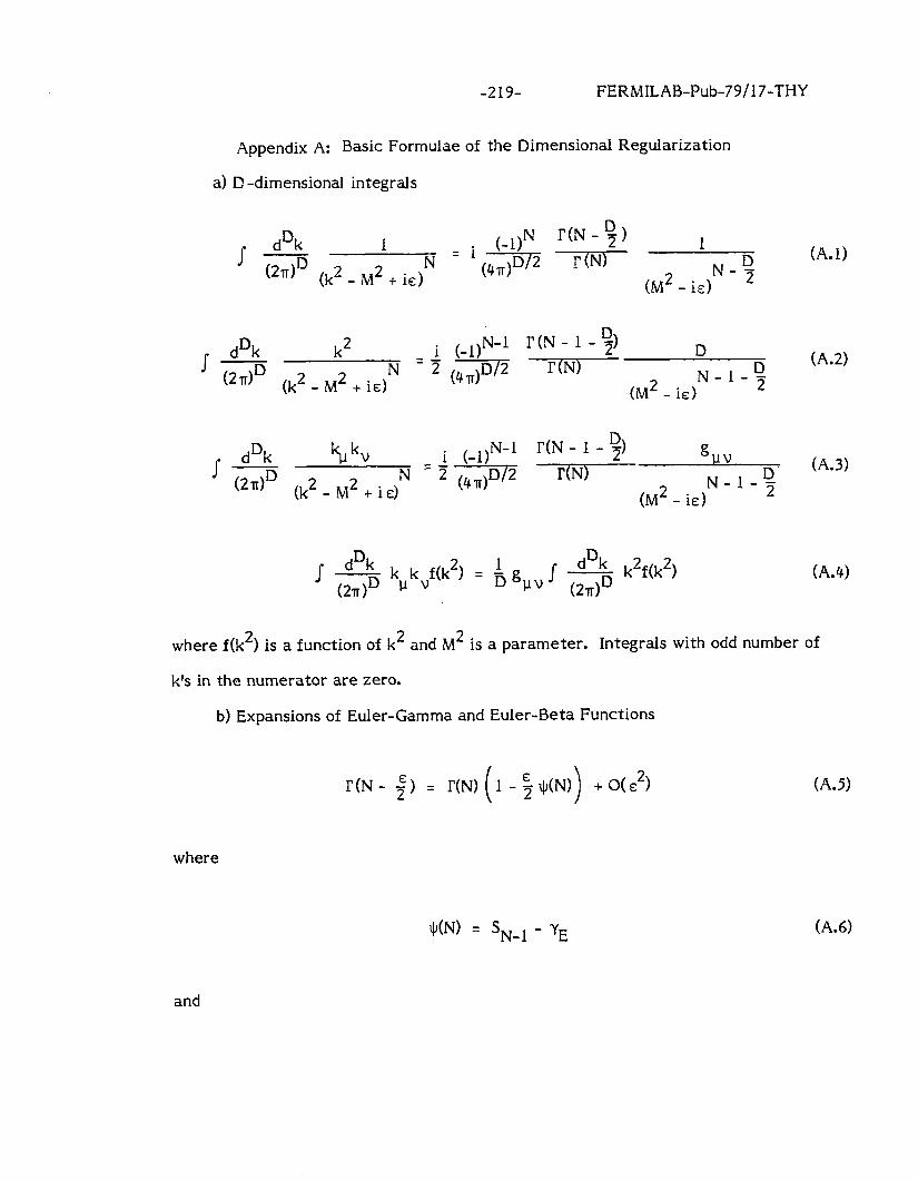
-219- FERMILAB-Pub-79/17-THY
Appendix A: Basic Formulae of the Dimensional Regularization
a) D-dimensional integrals
dDk I-----
1 ( l)N r(N-;)
(2T)D (k2 _ M2 + ic)N “($72 r(N)
1 D
(M2 _ ic)N - ’
dDk f-
k2 i (-l)N-1 r(N - 1 - $1 D
(2 dD (k2 - M2 + ic) N = 2 (z r(N)
(M2 - is) N-l-;
dDk s-
kc( kv i ( l)N-1 I’(N - 1 - ;I gull
(21dD (k2-M2+ic) N =q&pn r(N)
(M2 - ic) N-l-;
I L!%- k k (21TjD p v
f(k2) = h guy .f - dDk k2f(k2) (2dD
(A.11
(A-2)
(A.31
(A.41
where f(k2) is a function of k2 and M2 is a parameter. Integrals with odd number of
k’s in the numerator are zero.
b) Expansions of Euler-Gamma and Euler-Beta Functions
r(N- 2”) = l’(N)(l-5$(N)) +Ok2) (A.51
where
4’(N) = SN 1 - yE (A.6)
and
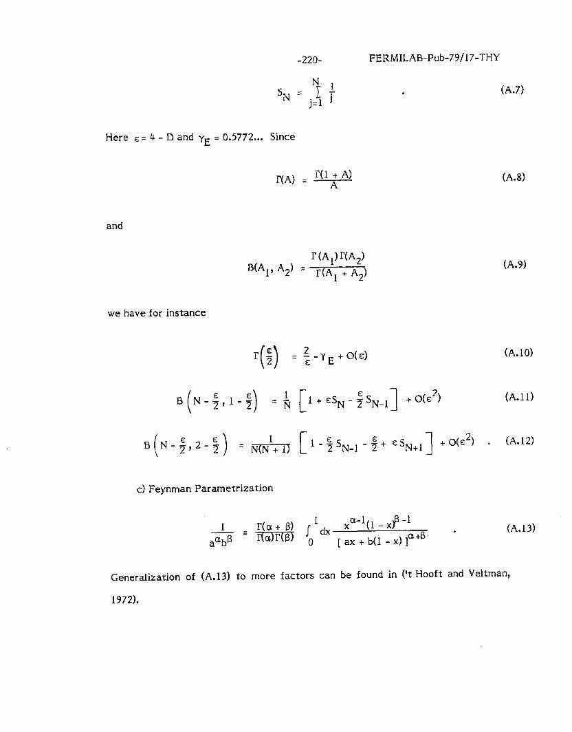
-220- FERMILAB-Pub-79/17-THY
Here E = 4 - D and yE = 0.5772... Since
I’(1 + A) r(A) = A
and
B(A1’ A2) = r (Al) lX42) r(A 1 + A2)
we have for instance
(A.8)
(A-9)
(A.lO)
(A.1 1)
l-$s~-l-$+ &-$+I. 3 + O(E2) l (A.12)
c) Feynman Parametrization
1 rb+ 8) sldx x a-1(1 - x)@ -1
-=-iTEmm o .
aClbB [ ax + b(l - x) ]a’B (A.13)
Generalization of (A.13) to more factors can be found in (‘t Hooft and Veltman,
1972).
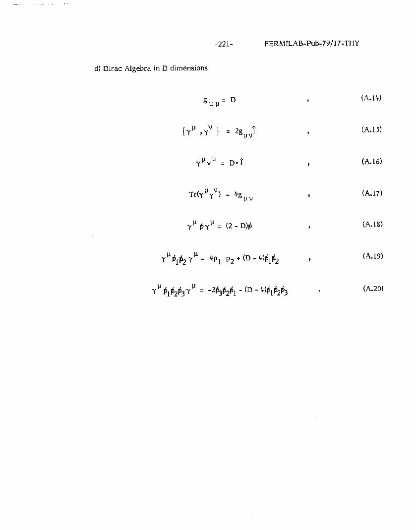
-221-
d) Dirac Algebra in D dimensions
FERMILAB-Pub-79/17-THY
gllv= D
YPYl-l = D-f
Tr(ypyv) = 4g,,.
y’fiy’= (2-D)$
YQlp2 YN = 4~1 p2 + (D - 4)hlb2 Y
Y ’ fil$2fi3 Y ’ = -2fi34Sl - (D - 4)hl&4 l
(A.14)
(A.15)
(~.16)
(A. 17)
(~.18)
(A.19)
(A.20)
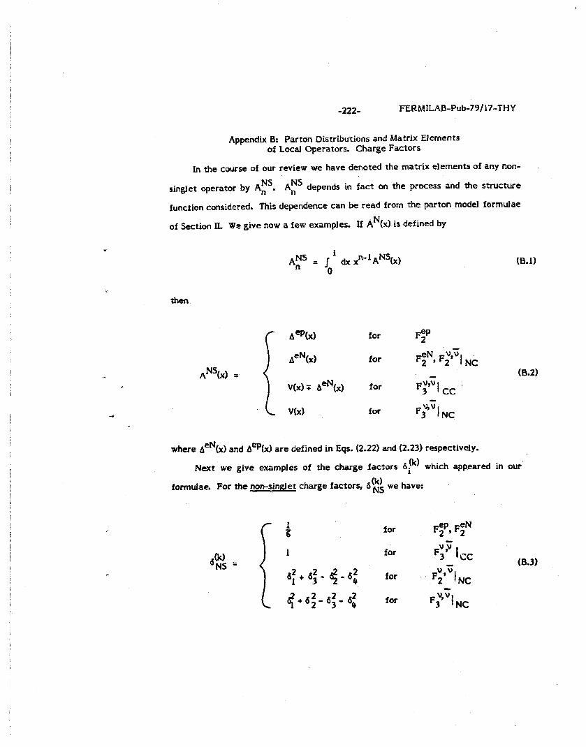
-222- FERMlLAB-Pub-79/17-THY
Appendix B: Parton Distributions and Matrix Elements of Local Operators. Charge Factors
h the course of our review we have denoted the matrix elements of any non-
NS singlet operator by A, . ANS n depends in fact on the process and the structure
function considered. This dependence can be read from the parton model formulae
of Section II. We give now a few examples. If AN(x) is defined by
(0.1)
then
AN’(x) = .I A epbd for Fep 2
AeN
V(x) 7 AeN
for
for
FeN - 2 ~Fzy’uIN~
(8.2) F$ CC
VW for
where AeN and Aep(x) are defined in Eqs. (2.22) and (2.23) respectively.
(k) Next we give examples of the charge factors Ai which appeared in our’
(k) formulae. For the non-singlet charge factors, 6 NS we have:
for FP, FzN
&k) NS =
for - (B-3)
for ,F;svt NC

-223-
(k) For the singlet charge factors, “J, , we have:
for
FERMILAB-&b-79/ i7-THY
Fep FeN 2’ 2
for FiSV CC . -1 (8.4)
for F;‘” NC -1
The formulae above are for the case of four flavors but it is a simple matter to
generalize them to any number of flavors.
The relations between A’,CQg) and part& distributions are given in Eqs.
(5.29) and (5.30). Combining these equations with Table ?I and the expectation
Az(Q$ > Az(QE) for n 24 we observe that AJQE) >> AA for n 14.
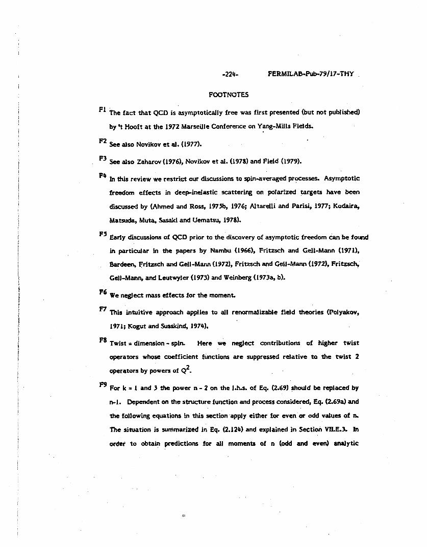
-224- FERMXLAB-Pub-79/J7-THY
FOOTNOTES
F1 The fact that QCD is ‘&ymptotically free was first presented (but not pubJished1
by ‘t Hooft at the 1972 Marseille Conference on Yang-Mills Fields. .
F2 See also Novikov et al. (1977).
F3 See also Zaharov (19761, Novikov et al. (1978) and Field (1979).
F4 In this review we restrict our discussions to spin-averaged processes. Asymptotic
freedom effects in deep-inelastic scattering on polarized targets have been
discussed by (Ahmed and Ross, 19754 1976; Altareili and Parisi, 1977; Kodaira,
Matsuda, Muta, Sasaki and Uematsu, 1978).
F5 Early discussions of QCD prior to the discovery of asymptotic freedom can be found
in particular in the papers by Nambu (19661, Fritxsch and Cell-Mann (19711,
Bardcen, Pritzsch and Cdl-Mann (19721, Fritzsch and Gell-Mann (1972& Fritzsch,
Cdl-Mann, and Leutwyler (1973) and Weinberg (1973a, b).
F6 We neglect mass effects for the moment.
F7 This intuitive approach applies to all renormalizable field theories (Polyakov,
1971; Kogut and Susskind, 1974).
F% Twist P dimension - spin. Here we neglect contributions of higher twist
operators whose coefficient functions are suppressed relative to the twist 2
operators by powers of Q2.
F9 For k = 1 and 3 the power n - 2 on the f.h.s. of Eq. (2.69) should be replaced by
n-l. Dependent on the structure function and process considered, Eq. (2.694 and
the following equations in this section .apply either for cvcn’or odd v&es of n.
The situation is summarized in Eq. (2.124) and explained in Section VlLE.3. In
order to obtain predictions for all moments of n (odd and evm) analytic
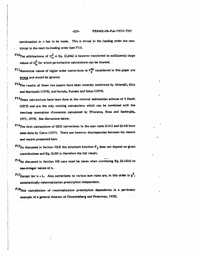
-22%. FERMILAB-Pub-79/17-THY
continuation in n has to be made. This is trivial in the leading order but non-
. trivial in the next-to-leading order (see F33).
i Fl%he arbitrariness of Qz in Eq. (2.69a) is however restricted to sufficiently large
i values of Qz for which perturbative calculations can be trusted .
j F1 lbjumerical values of higher order corrections to Fzp considered in this paper are
wrong and should be ignored.
I F12The results of these two papers have been recently confirmed by Altarelli, Ellis
and Martinelli (19791, and Harada, Kaneko and Sakai (1979).
I F1%hese calculations ha ve been done in the minimal subtraction scheme of ‘t Hooft
(1973) and are the only existing caldations which can be combined with the
two-loop anomalous dimensions calculated by (Floratos, Ross and Sachrajda,
1977, 1979). See discussions below.
F141he first calculations of QCD corrections to the sum rules (2.41) and Q-43) have L
I been done by Caivo (1977). There are however discrepancies between his results \-
and results presented here. -_
PlS i As discussed in Section VILE the structure function F3 does not depend on @on
contributions and Eq. (2.90) is therefore the full result. --.
F16As discussed in Section VIII care must be taken when continuing Eq. (2.lOlb) to
-integer values of n.
F17Except for k = L. Also corrections to various sum ruies are, in.this order in g2,
automatically renormalization prescription independent.
‘%his cancellation 0 f renormalization prescription dependence is a particular
example of a general theorem of (Stueckdberg &d Peterman, 1953). . . 3
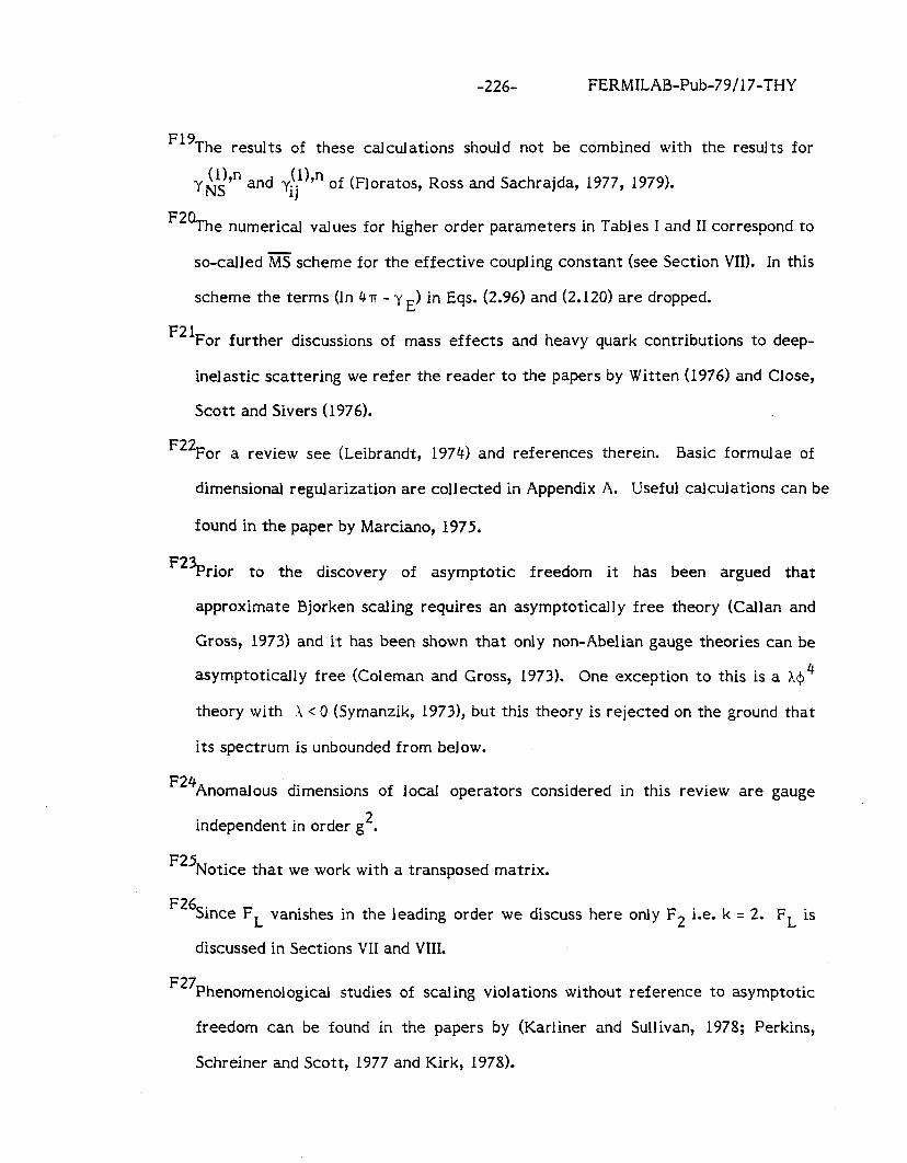
-226- FERMILAB-Pub-79/17-THY
F19 The results of these calculations should not be combined with the results for
(l),n yNS -’ and yi;’ ? of (Floratos, Ross and Sachrajda, 1977, 1979).
F20Th e numerical values for higher order parameters in Tables I and II correspond to
so-called MS scheme for the effective coupling constant (see Section VII). In this
scheme the terms (In HIT - y E) in Eqs. (2.96) and (2.120) are dropped.
F21 For further discussions of mass effects and heavy quark contributions to deep-
inelastic scattering we refer the reader to the papers by Witten (1976) and Close,
Scott and Sivers (1976).
F22 For a review see (Leibrandt, 1974) and references therein. Basic formulae of
dimensional regularization are collected in Appendix A. Useful calculations can be
found in the paper by Marciano, 1975.
F23p . rior to the discovery of asymptotic freedom it has been argued that
approximate Bjorken scaling requires an asymptotically free theory (Callan and
Gross, 1973) and it has been shown that only non-Abelian gauge theories can be
asymptotically free (Coleman and Gross, 1973). One exception
theory with X < 0 (Symanzik, 1973), but this theory is rejected on
its spectrum is unbounded from below.
to this is a Xo 4
the ground that
F24 Anomalous dimensions of local operators considered in this review are gauge
independent in order g2.
F25 Notice that we work with a transposed matrix.
F26Since FL vanishes in the leading order we discuss here only F2 i.e. k = 2. FL is
discussed in Sections VII and VIII.
F27 Phenomenological studies of scaling violations without reference to asymptotic
freedom can be found in the papers by (Karliner and Sullivan, 1978; Perkins,
Schreiner and Scott, 1977 and Kirk, 1978).
-227- FERibIILAB-Pub-79/17-THY
F2% or an excellent review of the deep-inelastic muon data we refer the reader to
the paper by (Francis and Kirk, 1979).
F29 For recent calculations of asymptotic freedom and W boson propagator effects at
very high energies (1 - 100 TeV) see the papers by HaIprin and Oakes (1979) and
Oakes and Tung (1978).
F3% should be emp hasized that the predictions of scalar theories as presented here
are based on an unproven assumption that perturbative calculations are reliable
for these theories. See discussion in Section V1.C.
F31See also Abbott (1979).
F32 Generalization of this proof to all orders in g2(Q2) has been discussed by Moshe
(1978) and Schellekens (1979). For a very nice discussion of this topic see
Peterman (1979).
F33 W,n It turns out that yNs = y”, + (-l)nyE where y”, and y”, may be analytically
continued in n. Because of the factor (-1)” the even and odd values of yNs (lh (see
F9) must be (in the process of inversion) analytically continued to u”, + y: and
Y; - yt respectively. The fact that y: f 0 can be related to flavor symmetry
breaking in antiquark distributions (Ross and Sachrajda, 1979).
F34 We recall that we have calculated the diagrams of Fig. 8 in Section III in order to
find yl,($, the coefficient of In -p2/u2 in Eq. (7.29). This time we are interested
(2),NS in the constant pieces An .
F35The parameters ENS k n correspond to the MS scheme of Eq. (7.58) and are obtained 9 from Eq. (7.42) by dropping there (In 41t - yE) terms. Notice that the n
dependence of An (k) is independent of the definition of g2(Q2).
-228- FERMILAB-Pub-79/17-THY
F36Similar conclusions have been reached by Anderson et al. (1979).
F37 The material of subsections VII1.B and VII1.D has been done in a collaboration
with W.A. Bardeen.
F38For n = 2, 4, 6, 8 and 10 the position of the singularity is at f = 5.583, 3.788,
1.627, 0.142 and -0.988 respectively. The corresponding residue in R; tn are equal
to -15.43, 1.36, 0.2, 0.007 and -0.02.
F39 Notice that the diagrams of Fig. 10b enter also the calculation of yg in which
case one is interested only in the coefficient of In -p2/p2 (see Eq. 8.52). This (2) $J time we are interested in the constant pieces AnG .
F40 See Appendix B.
F41 While completing this review we received a paper by (Anderson et al., 1979) where
a comparison of higher order corrections with the measured moments of F;P and
Fid has been done. The agreement with the data is good with the value of bMS =
0.459 + 0.111. This is consistent with the value obtained from the analysis of
non-singlet structure functions (Eq. 7.59).
F42See Nanopoul os and Ross (1975). For a recent analysis see (Abbott, Atwood and Barnett, 197!?1.
F43 Strictly speaking the diagrams of Fig. 36 represent the contribution of the
photon-quark scattering to the photon-proton cross-section. In order to calculate
the full photon-proton cross-section also the contribution of the photon gluon
scattering has to be considered (see Section VIII).
F44See also Keller, Walsh and Zerwas (1978) and Kajantie (1979). Gunion and Jones (1979)
F45 have discussed the parameter nn in the intuitive approach.
See for instance Ellis, Georgi, Machacek, Politzer and Ross (1979) except that we
denote differential cross-sections as do/dx by o(x), do/(dxdz) by o(x, z) etc. For
simplicity and following these authors we consider only the cross-sections which
are projected out by contracting the indices of the virtual photon with the tensor
-229- FERMILAB-Pub-79/17-THY
F46p revious studies of the fragmentation functions in the context of QCD can be
found in Callan and Goldberger (1975) and Mueller (1974). Semi-inclusive deep-
inelastic scattering has been discussed previously by many authors, in particular
by Georgi and Politzer (1978 a) and by Mendez (1978).
F47Some of the order g2 corrections to e+e- + h(P) + anything are shown in Fig. 44.
F481n th’ IS example we do not discuss the g2 corrections which arise from gluon
production and its subsequent decay into hadrons.
-230- FERMILAB-Pub-79/17-THY
REFERENCES
Abad,J. and B. Humpert, 1978, Phys. Lett. 77B, 105.
Abad, J. and 8. Humpert, 1979, Phys. Lett. 80B, 286.
Abarbanel, H.D.I., 1974, SLAC Report No. 179, Volume 1, 399.
Abbott, L.F., and R.M. Barnett, 1979, SLAC-PUB-2325.
Abbott, L.F., 1979, SLAC-PUB-2296.
Abbott, L.F., E.L. Berger, R. Blankenbecler and G. Kane, 1979, SLAC-PUB-2327.
Abbott, L.F., W.B. Atwood and R.M. Barnett, 1979, SLAC-PUB-2374).
Abers, ES., and B.W. Lee, 1973, Physics Reports 9C, 1.
Adler, S.L., 1966, Phys. Rev. 143, 1144.
Ahmed, M.A., and G.G. Ross, 1975a, Phys. Lett. 59B, 369.
Ahmed, M.A., and G.G. Ross, 1975b, Phys. Lett. 56B, 385.
Ahmed, M.A., and G.G. Ross, 1976, Nucl. Phys. Bill, 441.
Albright, C., and R. Shrock, 1977, Phys. Rev. D16, 575.
Altarelli, G., G. Parisi, and R. Petronzio, 1976, Phys. Lett. 63B, 183.
Altarelli, G., 1978a, “Partons in Quantum Chromodynamics” Roma preprint, 701.
Altarelli, G., 1978b, Roma preprint, 714.
Altarelli, G., and G. Parisi, 1977, Nucl. Phys. 8126, 298.
Aitarelli, G., R.K. Ellis and G. Martinelli, 1978, Nucl. Phys. B143, 521 and Erratum
Nucl. Phys. B146, 544.
Altarelli, G., R.K. Ellis and G. Martinelli, 1979a, MIT preprint, MIT-CTP-776.
Altarelli, G., R.K. Ellis, G. Martinelli and S.Y. Pi, 1979b, MIT preprint MIT-CTP-793.
Amati, D., R. Petronzio and G. Veneziano, 1978a, Nucl. Phys. B140, re.
Amati, D., R. Petronzio and G. Veneziano, 1978b, Nucl. Phys. B146, 29.
Anderson, H.L., et al., 1977, Phys. Rev. Lett. 38, 1450.
Anderson, H.L., H.S. Matis, and L.C. Myrianthopoulos, 1978, Phys. Rev. Lett. 40,
1061.
Anderson, H.L., et al., 1979, Fermilab-Pub-79/30-EXP.
-231- FERMILAB-79/17-THY
Andrei, J., and D.J. Gross, 1978, Phys, Rev. Dl8, 468.
Asratyan, A.E., et al., 1978, Phys. Lett. 76B, 239.
Appelquist, T., and H. Georgi, 1973, Phys. Rev. D8, 4000.
Appelquist, T., and R. Shankar, 1978, Phys. Lett. 78B, 468.
Atwood, W.B., et al., 1976, Phys. Lett. 64B, 479.
AvQez, c., G. Cocho and M. Moreno, 1977, UNAM-preprint, INFUNAM-77-30.
Bac& M., 1978, Phys. Lett. 78B, 132.
Baier, R., and K. Fey, 1979, Bielefeld preprint BJ-TP 79/11.
Bailin, D., A. Love, and D. Nanopoulos, 1974, Lett. Nuovo Cimento 9, 501.
Ball, R.C., et al., 1979, Phys. Rev. Lett. 42, 866.
Baluni, V., and E. Eichten, 1976a, Phys. Rev. Lett. 37, 1181.
Baluni, V., and E. Eichten, 1976b, Phys. Rev. D14, 3045.
Baranov, D.S., et al., 1978, Phys. Lett. 76B, 366.
Barbieri, R., J. Ellis, M.K. Gaillard and G.G. Ross, 1976a, Phys. Lett. 64B, 171.
Barbieri, R., J. Ellis, M.K. Gaillard and G.G. Ross, 1976b, Nud. Phys. B117, 50.
Barbieri, R., and R. Gatto, 1977, Phys. Lett. 66B, 181.
Barbieri, R., L. Caneschi, G. Curci and E. d’Emilio, 1979, Phys. Lett. 81B, 207.
Bardeen, W.A., H. Fritzsch and M. Gell-Mann, 1972, in ?xale and Conformal
Symmetry in Hadron Physics,” edited by R. Gatto (Wiley, New York).
Bardeen, W.A., A.J. Buras, D.W. Duke, and T. Muta, 1978, Phys. Rev. D18, 3998.
Bardeen, W.A., and A.J. Buras, 1979a, Phys. Rev. D20, 166.
Bardeen, W.A., and A.J. But-as, 1979b, Fermilab-Pub-79/31-THY.
Barger, V., and R.J.N. Phillips, 1974, Nud. Phys. B73, 269.
Barger, V., and R.J.N. Phillips, 1978, Nucl. Phys. B132, 531.
Barish, B.C., et al., 1977a, Phys. Rev. Lett. 38, 314.
Barish, B.C.: et al., 1977b, Phys. Rev. Lett. 39, 1595.
Barish, B.C., et al., 1978, Phys. Rev. Lett. 40, 1414.
-232- FERMILAB-Pub-79/17-THY
Barnett, R.M., 1976, Phys. Rev. D14, 70.
Barnett, R.M., H. Georgi, and H.D. Politzer, 1976, Phys. Rev. Lett. 37, 1313.
Barnett, R.M., and F. Martin, 1977, Phys. Rev. D16, 2765.
Baul ieu, L., and C. I<ounnas, 1978, Nucl. Phys. B141, 423.
Baulieu, L., J. Ellis, M.K. Gaillard, 1978, Phys. Lett. 77B, 280.
Benvenuti, A., et al., 1979, Phys. Rev. Lett. 42, 149.
Berge, J.P., et al., 1976, Phys. Rev. Lett. 36, 639.
Berger, E.L., 1979, SLAC-PUB-2314.
Bitar,K., P.W. Johnson and W.K. Tung, 1979, Phys. Lett. 83B, 114.
Bjorken, J.D., and S. D. Drell, 1965, Relativistic Quantum Fields, McGraw-Hill
Book Company.
Bjorken, J.D., 1967, Phys. Rev. 163, 1767.
Bjorken, J.D., 1969, Phys. Rev. 179, 1547.
Bjorken, J.D., and E.A. Paschos, 1969, Phys. Rev. 185, 1975.
Bjorken, J.D., and E.A. Paschos, 1970, Phys. Rev. Dl, 3151.
Bodek, A., et al., 1979, SLAC-PUB-2248.
Bogolubov, N.N., and D.V. Shirkov, 1959, Introduction to the theory of quantized
fields (Interscience, N.Y .).
Bosetti, P.C., et al., 1977, Phys. Lett. 708, 273.
Bosetti, P.C., et al., 1978, Nucl. Phys. 8142, 1.
Broadhurst, D.J., 1975, Open University preprint, 4102-l (unpublished).
Brodsky, S.J., T. Kinoshita, and H. Terazawa, 1971, Phys. Rev. Lett. 27, 280.
Brodsky, S.J., T. De Grand, J.F. Gunion and J. Weis, 1978, Phys. Rev. Lett. 41, 672.
Brodsky, S.J., 1978, SLAC-PUB-2217.
Brodsky, S.J., T. De Grand, J.F. Gunion and J. Weis, 1979, Phys. Rev. D19, 1418.
Brodsky, S.J., and J.F. Gunion, 1979, Phys. Rev. D19, 1005.
Brown, L.S., 1979, University of Washington preprint, RLO-1388-777.
-233- FERMILAB-Pub-79/17-THY
Budnev, V., I. Ginzburg, G. Meledin and V. Serbo, 1975, Physics Reports 1X, 182.
Bukhvostov, L.N. Lipatov, and Popov, 1975, Sov. J. Nucl. Phys., Vol. 20, 287.
Buras, A.J., 1977, Nucl. Phys. B125, 125.
Buras, A.J., and K.J.F. Gaemers, 1977, Phys. Lett. 71B, 186.
Buras, A.J., and K.J.F. Gaemers, 1978, Nucl. Phys. B132, 249.
Buras, A.J., E.G. Floratos, D.A. Ross, and C.T. Sachrajda, 1977, Nucl. Phys. B131,
308.
Buras, A.%, and D.W. Duke, 1978, unpublished.
But-as, A.J., 1979, Fermilab-Conf-79/65-THY, to appear in the Proceedings of the
Boulder Summerschool, 1979.
Cabibbo, N., and R. Petronzio, 1978, Nucl. Phys. B137, 395.
Callan, C.G., and D.J. Gross, 1969, Phys. Rev. Lett. 22, 156.
Callan, C.G., 1970, Phys. Rev. D2, 1541.
Callan, C.G., 1972, Phys. Rev. D5, 3202.
Callan, C.G., and D.J. Gross, 1973, Phys. Rev. D8, 4383.
Callan, C.G., and M. Goldberger, 1975, Phys. Rev. Dll, 1553.
Calvo, M., 1977, Phys. Rev. D15, 730.
Carlitz, R.D., and C. Lee, 1978, Phys. Rev. D17, 3238.
Caswell, W., and F. Wilczek, 1974, Phys. Lett. B49, 291.
Caswell, W., 1974, Phys. Rev. Lett. 33, 244.
Celemaster, W., and R.J. Gonsalves, 1979, Phys. Rev. Lett. 42, 1435.
Celemaster, W., and R.J. Consalves, work in progress.
Christ, N., 8. Hassiacher, and A. Mueller, 1972, Phys. Rev. D6, 3543.
Close, F.E., D.H. Scott and D. Sivers, 1976, Nucl. Phys. B117, 134.
Close, F-E., 1979, An Introduction to Quarks and Partons, Academic Press.
Coleman, S., 1971, Lectures given at 9th Ettore Majorana School for Subnuclear
Physics, Erice, p. 359, 605.
Coleman, S., and D.J. Gross, 1973, Phys. Rev. Lett. 31, 851.
-234- FERMILAB-Pub-79 /17-THY
Collins, J-C-, and A.J. Macfarlane, 1974, Phys. Rev. DlO, 1201.
Combridge, B.L., J. Kripfganz, and J. Ranft, 1977, Phys. Lett. 71X3, 234.
Contogouris, A.P., and J. Kripfganz, 1979a, Phys. Lett. 848, 473.
Contogouris, A.P., and J. Kripfganz, 1979b, McGill University preprint.
Contogouris, A.P., R. Gaskell, and S. Papadopoulos, 1978, Phys. Rev. D17, 2314.
Cornwall, J.M., and R.E. Norton, 1969, Phys. Rev. 177, 2584.
Crewther, R.J., 1976, Cargese 1975, ed. by M. Levy, J. Basdevant, D. Speiser and
R. Gastmans, p. 345.
Cutler, R., and D. Sivers, 1977, Phys. Rev. D16, 679.
Dash, J., 1972, Nucl. Phys. B47, 269.
Deden, H., et al., 1975, Nucl. Phys. B85, 269.
De Grand, T.A., 1978, Santa Barbara preprint UCSB, TH-15.
De Groot, J.G.H., et al., 1979a, Zeitschrift fur Physik C, Volume 1, 143.
De Groot, J.G.H., et al., 1979b, CERN preprint 79-0133.
De Groot, J.G.H., et al., 1979c, CERN preprint 79-0168.
De Rafael, E., 1977, Lectures on Quantum Electrodynamics, Universidad Autonoma
de Barcelona.
De Rujula, A., H. Georgi, and H.D. Politzer, 1974, Phys. Rev. DlO, 2141.
De Rujula, A., H. Georgi, and H.D. Politzer, 1977a, Ann. of Phys. 103, 315.
De Rujula, A., H. Georgi, and H.D. Politzer, 1977b, Phys. Rev. D15, 2495.
De Rujula, A., J. Ellis, E.G. Floratos and M.K. Gaillard, 1978, Nucl. Phys. B138,
387.
De Witt, R.J., L.M. Jones, J.D. Sullivan, D.E. Willen and H.W. Wyld, Jr., 1979, Phys.
Rev. DlY, 2046.
Dine, M., and J. Sapirstein, 1979, work in progress.
Dokshitser, Yu. L., 1977, Leningrad preprint 330.
Dokshitser, Yu. L., D.I. Dyakanov, and S.I. Troyan, 1978a, SLAC-TRANS-183.
Dokshitser, Y u. L., D.I. Dyakanov, and S.I. Troyan, 1978b, Phys. Lett. 79B, 269,
290.
-235- FERMILAB-Pub-79/17-THY
Drell, S.D., D. Levy and T. Yan, 1969, Phys. Rev. 187, 2159.
Drell, S.D., and T. Yan, 1971, Ann. Phys. (N.Y.) 66, 578.
Duke,D.W., and R.G. Roberts, 1979a, Rutherford Lab Report, RL-79-025.
Duke,D.W., and R.G. Roberts, 1979b, in preparation.
Eichten, T., et al., 1973, Phys. Lett. 46B, 281.
Einhorn, M., and B. Weeks, 1978, SLAC-PUB-2164.
Ellis, J., 1976, in lectures on Weak and Electromagnetic Interactions at High
Energy, Les Houches, 1976, ed. by R. Balian and C.H. Llewellyn-Smith.
Ellis, J., 1978a, SLAC-PUB-2121.
Ellis, J., 1978b, SLAC-PUB-2177.
Ellis, J., M.K. Gaillard and W. Zakrzewski, 1979, CERN preprint TH-2595.
Ellis, J., M.K. Gaillard and G.G. Ross, 1976, Nucl. Phys. Bill, 253 and Erratum,
Nucl. Phys. B130, 516.
Ellis, R.K., R. Petronzio, and G. Parisi, 1976, Phys. Lett. 64B, 97.
Ellis, R.K., H. Georgi, M. Machacek, H.D. Politzer and G.G. Ross, 1978, Phys.
Lett. 78B, 281.
Ellis, R.K., H. Georgi, M. Machacek, H.D. Politzer and G.G. Ross, 1979, CALT-68-
684.
Farhi, E., 1977, Phys. Rev. Lett. 39, 1587.
Feldman, G.J., 1979, Proceedings of the 19th International Conference on High En-
ergy Physics, Tokyo 1978. Edited by S. Homma, M. Kawaguchi, H. Miyazawa,
p. 777.
Feynman, R.P., 1969, Phys. Rev. Lett. 23, 1415.
Feynman, R.P., 1972, “Photon-Hadron Interactions,‘! W.A. Benjamin, New York.
FieJd,R.D., and R.P. Feynman, 1977, Phys. Rev. D15, 2590.
Field,R.D., 1978, Phys. Rev. Lett. 40, 997.
Field,R.D., 1979, Proceedings of the 19th International Conference on High Energy
Physics, Tokyo 1978. Edited by S. Homma, hl. Kawaguchi, H. Miyazawa, p.
743.
-236- FERMILAB-Pub-79/17-THY
Field, R.D., and D.A. Ross, 1979, work in progress.
Floratos, E.G., 1978, Nuovo Cimento 43A, 241.
Floratos, E.G., D.A. Ross, and C.T. Sachrajda, 1977, Nucl. Phys. B129, 66 and
Erratum, Nucl. Phys. B139, 545.
Floratos, E.G., D.A. Ross, and C.T. Sachrajda, 1979, CERN preprint TH-2566.
Fox, G., 1977, Nucl. Phys. B131, 107.
Fox, G., 1978a, Nucl. Phys. B134, 269.
Fox, G., 1978b, Proceedings of 11Neutrinos-78,” 137, edited by E.C. Fowler.
Fox, G., and S. Wolfram, 1979, Nucl. Phys. B149, 413.
Francis, W.R., and T.B.W. Kirk, 1979, Fermilab report, to be published in Physics
Reports.
Frazer, W.R., and J.F. Gunion, 1979a, UCSD-lOPlO-194.
Frazer, W.R., and J.F. Gunion, 1979b, UCSD-78-5.
Fritzsch, H., and M. Cell-Mann, 1971, in Proceedings of the International
Conference on Duality and Symmetry in High Energy Physics, edited by
E. Gotsman (Weizmann, Jerusalem),
Fritzsch, H., and M. Gell-Mann, 1972, Proceedings of the XVI International
Conference on High Energy Physics, Vol. 2, p. 135 (National Accelerator
Laboratory).
Fritzsch, H., M. Gell-Mann, and H. Leutwyler, 1973, Phys. Lett. B74, 365.
Fritzsch, H., and K.H. Streng, 1978, Phys. Lett. 74B, 90.
Furmanski, W., 1978, Phys. Lett. 77B, 3 12.
Furmanski, W., and S. Pokorski, 1979a, CERN preprint TH-2665.
Furmanski, W., and S. Pokorski, 1979b, CERN preprint.
Furmanski, W., 1979, CERN preprint TH-2664.
-237- FERMILAB-Pub-79/17-THY
Gaillard, M.K., 1977, Proceedings of the 12th Recontre de Moriond, Vol. 1, p. 485,
edited by J. Tran Thanh Van.
Cell-Mann, M., and F. Low, 1954, Phys. Rev. 95, 1300.
Georgi, H., and H.D. Politzer, 1974, Phys. Rev. DV, 416.
Georgi, H., and H.D. Politzer, 1976, Phys. Rev. D14, 1829.
Georgi, H., and M. Machacek, 1977, Phys. Rev. Lett. 39, 1587.
Georgi, H., and H.D. Politzer, 1978a, Phys. Rev. Lett. 40, 3.
Georgi, H., and H.D. Politzer, 1978b, Nucl. Phys. B136, 445.
Glashow, S.L., J. Iliopoulos and L. Maiani, 1970, Phys. Rev. D2, 1285.
Gliick, M., and E. Reya, 1976, Phys. Lett. 64B, 169.
Cluck, M., and E. Reya, 1977a, Phys. Rev. D16, 3242.
Gliick, M., and E. Reya, 1977b, Nucl. Phys. B130, 76.
Click, M., and E. Reya, 1979, Desy preprint 79/13.
Gonzalez-Arroyo, A., C. Lopez and F.J. Yndurain, 1978, FTUAM 78-6.
Gordon, B.A., et al., 1978, Phys. Rev. Lett. 41, 615.
Gottlieb, J., 1978, Nucl. Phys. 139, 125.
Graham, R.H., E.M. Haacke, and P. Savaria, 1979, Phys. Rev. DlY, 112.
Gribov, V.N., and L.N. Lipatov, 1972, Soviet J. Nucl. Phys. 15, 438, 675.
Gross, D.J., and F. Wilczek, 1973a, Phys. Rev. Lett. 30, 1323.
Gross, D.J., and F. Wilczek, 1973b, Phys. Rev. D8, 3633.
Gross, D.J., and F. Wilczek, 1974, Phys. Rev. DY, 980.
Gross, D.J., 1974, Phys. Rev. Lett. 32, 1071.
Gross, D.J., S.B. Treiman and F. Wilczek, 1976, Phys. Rev. D15, 2486.
Gross, D.J., and C.H. Llewellyn-Smith, 1969, Nucl. Phys. B14, 337.
Gross, D.J., 1976, in Methods in Field Theory, Les Houches 1975, edited by R. Balin
and J. Zinn-Justin (North-Holland, Amsterdam), chap. 4.
Gunion, J.F., and D. Jones, 1979, University Davis preprint UCD-79-2.
-238- FERMILAB-Pub-79 /17-THY
Gupta, S., and A.H. Mueller, 1979, Phys. Rev. D20, 118.
Halprin, A., 1978, Proceedings of 1978 DUMAND Summer Workshop.
Halprin, A., and R.J. Oakes, 1979, Fermilab-Conf-79.15-THY.
Halzen, F., 1979, Proceedings of 19th International Conference on High Energy
Physics, Tokyo 1978. Edited by S. Homma, M. Kawaguchi, H. Miyazawa, p. 214.
Harada, K., T. Kaneko, and N. Sakai, 1979, Nucl. Phys. B155, 169.
Harari, H., 1979, SLAC-PUB-2254.
Hill, Ch. T., and G.G. Ross, 1979, Nucl. Phys. B148, 373.
Hinchliffe, I., and C.H. Llewellyn-Smith, 1977a, Nucl. Phys. B128, 93.
Hinchliffe, I., and C.H. Llewellyn-Smith, 1977b, Phys. Lett. 66B, 281.
Hinchliffe, I., and C.H. Llewellyn-Smith, 1977c, Phys. Lett. 70B, 247.
Hwa, R., 1978, Thirteenth Rencontre de Moriond, ed. by J. Tran Thanh Van, p. 197.
Jaffe, R.L., 1972, Phys. Rev. D5, 2622.
Johnson, P.W., and W.K. Tung, 1977a, Phys. Rev. D16, 2767.
Johnson, P.W., and W.K. Tung, 1977b, Nud. Phys. B121, 270.
Johnson, P.W., and W.K. Tung, 1979, Illinois Institute of Technology preprint.
Jones, D.R.T., 1974, Nud. Phys. 875, 531.
Jost, R., and J.M. Luttinger, 1950, Helv. Phys. Acta 23, 201.
Kaplan, J., and F. Martin, 1976, Nucl. Phys. BlI5, 333.
Kajantie, K., 1979, Helsinki University preprints HU-TFT-78-30, HU-TFT-79-5.
Karliner, I., and J.D. Sullivan, 1978, Phys. Rev. D18, 3202.
Kazama, Y., and Y.P. Yao, 1978, Phys. Lett. 41, 611.
Kazama, Y., and Y.P. Yao, 1979, Phys. Rev. DlY, 3111, 3121.
Kings1 ey, R.L., 1973, Nucl. Phys. B60, 45.
Kirk, T.B.W., 1978, Fermilab Tech. Memo TH-791.
Kodaira, J., and T. Uematsu, 1978, Nucl. Phys. B141, 497.
Kodaira, J., S. Matsuda, T. Muta, K. Sasaki, and T. Uematsu, 197% Phys.
Rev. D20, No. 4. Kodaira, J., S. Matsuda, K. Sasaki and T. Uematsu, 1979b, Kyoto University preprint,
RIFP-360.
-239- FERMILAB-Pub-79 /17-THY
Kogut, J., and L. Susskind, 1974, Phys. Rev. DY, 697, 706, 3391.
Kogut, J., and Shigemitsu, 1977, Phys. Lett. 718, 165.
Keller, K., and T.F. Walsh, 1977, Phys. Lett. 72B, 227.
Keller, K., T.F. Walsh, and P.M. Zerwas, 1978, Desy preprint 78/77.
Konishi, K., A. Ukawa, and G. Veneziano, 1978, Phys. Lett. 78B, 243.
Kripfganz, J., 1979, Phys. Lett. 828, 79.
Kubar-Andre’, J., and F.E. Paige, 1979, Phys. Rev. DlY, 221.
Kuti, J., and V.F. Weisskopf, 1971, Phys. Rev. D4, 3418.
Landshoff, P.V., and J.C. Polkinghorne, 1972, Phys. Reports 4C, 1.
Lautrup, B., 1976, Cargese 1975, ed. by M. Levy, J. Basdevant, D. Speiser and
R. Gastmans, p. 1.
Leibbrandt, G., 1975, Reviews of Modern Physics 47, 849.
Libby, S.B., and G. Sterman, 1978, Phys. Rev. D18, 3252, 4737.
Lipatov, L.N., 1975, Sov. J. Nucl. Phys. Vol. 20, 94.
Llewellyn-Smith, C.H., 1972, Physics Reports 3C, 261.
Llewellyn-Smith, C.H., 1975, Proceedings of the International Symposium on
Lepton and Photon Interactions at High Energies, Stanford.
Llewellyn-Smith, C.H., 1978a, Oxford preprint 2/78=
Llewell yn-Smith, C.H., 1978b, Acta Physica Austriaca, suppl. XIX, 331 l
Llewellyn-Smith, C.H., 1978c, Phys. Lett. 79B,83=
Marciano, W.J., 1975, Phys. Rev. D12, 3861.
Marciano, W. J., and H. Pagels, 1978, Physics Reports 36C, 137.
Martin, F., 1978, SLAC-PUB-2192.
Mendez, A., 1978, Nucl. Phys. B145, 199.
Mestayer, M., 1978, SLAC report 214.
Moorhouse, R-G., M.R. Pennington and G.G. Ross, 1977, Nucl. Phys. B124, 285.
-240- FERMILAB-Pub-79/17-THY
Moshe, M., 1978, Phys. Lett. 79B, 88, and Erratum, Phys. Lett. 808, 433.
Mueller, A.H., 1974, Phys. Rev. DY, 963.
Mueller, A.H., 1978, Phys. Rev. D18, 3705.
Muta,T;, 1979, Phys. Rev. D20, No. 5.
Nachtmann, O., 1973, Nucl. Phys. B63, 237.
Nachtmann, O., 1974, Nucl. Phys. B78, 455.
Nachtmann, O., 1977, in Proceedings of the International Symposium on Lepton and
Photon Interactions at High Energies, Hamburg 1977, edited by F. Gutbrod.
Nambu, Y., 1966, in Preludes in Theoretical Physics, edited by A. de Shalit (North-
Holland, Amsterdam).
Nanopoulos, D., and G. Ross, 1975, Phys. Lett. 58B, 105.
Novikov, V.A., L.B. Okun, M.A. Shifman, A.I. Vainstein, M.B. Voloshin, and
V.I. Zaharov, 1978, Physics Reports 41C, 1.
Novikov, V.A., M.A. Shifman, A.I.Vainstein and V.I. Zaharov, 1977, Annals of
Physics, 105, 276.
Oakes, R.J., and W.K. Tung, 1978, Fermilab-Conf-78/93-THY.
Owens, J.F., and E. Reya, 1978, Phys. Rev. D17, 3003.
Owens, J.F., 1978, Phys. Lett. 76B, 85.
Parisi, G., 1973, Phys. Lett. 43B, 207.
Parisi, G., 1975, Proc. 11th Rencontre de Moriond, ed. by J. Tran Thanh Van.
Parisi, G., and R. Petronzio, 1976, Physics Letters 62B, 331.
Parisi, G., and N. Sourlas, 1979, Nucl. Phys. B151, 421.
Perkins, D.H., P. Schreiner and W.G. Scott, Phys. Lett. 678, 347.
4.. 1979, CERN preprint TH-2581, to appear in Physics Reports.
-I 5. Weinberg 1976, Phys. Rev. D13, 1958.
- ‘0, 1346.
-241- FERMILAB-Pub-79/17-THY
Politzer, H.D., 1977a, Nucl. Phys. B129, 301.
Politzer, H.D., 1977b, Physics Lett. 70B, 430.
Politzer, H.D., 1979, Proceedings of 19th International Conference on High Energy
Physics, Tokyo 1978. Edited by S. Homma, M. Kawaguchi, H. Miyazawa, p. 229.
Polyakov, A.M., 1971, JEPT 32, 296.
Reya,E., 1979, Phys. Lett. 84B, 445.
Riordan, E.M., et al., 1975, SLAC-PUB-1634.
Ross, D.A., 1979, Acta Physica Polonica 810, 189.
Ross, D.A., and C.T. Sachrajda, 1979, Nucl. Phys. B149, 497.
Ross, D.A., A. Terrano and S. Wolfram, 1979, work in progress.
Roy, D.P., S. Paranjape, P.N. Pandita, and D.K. Choudhury, 1977, Tata Institute
preprint 094 1.
Sachrajda, C.T., 1978a, Phys. Lett. 73B, 185.
Sachrajda, C.T., 1978b, Phys. Lett. 76B, 100.
Sachrajda, C.T., 1978c, Thirteenth Rencontre de Moriond, ed. by J. Tran Than Van,
p. 17.
Sakai, N., 1979, CERN preprint TH-2641.
Salam, A., 1968, Proceedings of the 8th Nobel Symposium.
Schellekens, A.N., 1979, Nuovo Cim. Letters 24, 513.
Schellekens, AN., and W.L. Van Neerven, 1979, THEF-NYM-79.8.
Schmidt, LA., and R. Blankenbecler, 1977, Phys. Rev. D16, 1318.
Schnitzer, 1971, Phys. Rev. D4, 1429.
Shankar, R., 1977, Phys. Rev. D15, 755.
Sheiman, J., 1979, Nucl. Phys. B152, 273.
Shifman, M.A., A.I. Vainshtein and V.I. Zaharov, 1979, Nucl. Phys. 147B, 385.
Shizuya, K.I., and S.H.-H. Tye, Fermilab-Pub-79/16-THY.
Sterman, G., and S. Weinberg, 1977, Phys Rev. Lett. 39, 1436.
Stueckelberg, E.C.G., and A. Peterman, 1953, Helv. Phys. Acta 26, 499.
-242- FERMILAB-Pub-79/17-THY
Symanzik, K., 1970, Commun. Math. Phys. 18, 227.
Symanzik, K., 1973, Lett. Nuovo Cimento 6, 77.
Taylor, J.C., 1975, Proceedings of the International Symposium on Lepton and
Photon Interactions at High Energies, Stanford.
Taylor, J.C., 1976, “Gauge Theories of Weak Interactions,” Cambridge University
Press.
Terazawa, H., 1973, Rev. Mod. Phys. 45, 615.
‘t Hooft, G., 1973, Nucl. Phys. B61, 455.
‘t Hooft, G., and M. Veltman, 1972, Nucl. Phys. B44, 189.
‘t Hooft, G., and M. Veltman, 1973, “Diagrammar,” CERN Yellow report, CERN 73-
9.
Tittel, K., 1979, Proceedings of 19th International Conference on High Energy Phys-
ics, Tokyo 1978. Edited by S. Homma, M. Kawaguchi, H. Miyazawa, p. 863.
Tung, W.K., 1975, Phys. Rev. D12, 3613.
Tung, W.K., 1978, Phys. Rev. D17, 738.
Uematsu, T., 1978, Phys. Lett. 79B, 97.
Veneziano, G., 1979, Proceedings of 19th International Conference on High Energy
Physics, Tokyo 1978. Edited by S. Homma, M. Kawaguchi, H. Miyazawa, p. 725.
Walsh, T.F., and P. Zerwas, 1973, Phys. Lett. 44B, 195.
Wandzura, S., 1977, Nucl. Phys. B122, 412.
Watanabe, Y., et al., 1975, Phys. Rev. Lett. 35, 898, 901.
Weinberg, S., 1967, Phys. Rev. Lett. 19, 1264.
Weinberg, S., 1973a, Phys. Rev. Lett. 31, 494.
Weinberg, S., 1973b, Phys. Rev. D8, 4482.
Wilson, K., 1969, Phys. Rev. 179, 1499.
Witten, E., 1976, Nucl. Phys. B104, 445.
Witten, E., 1977, Nucl. Phys. B120, 189.
-243- FERMILAB-Pub-79/17-THY
Yndurain, F.J., 1978, Phys. Lett. 74B, 68.
Zaharov, V.I., 1976, ITEP-127.
Zee, A., 1973, Phys. Rev. D8, 4038.
Zee, A., F. Wilczek, and S.B. Treiman, 1974, Phys. Rev. DlO, 2881.
Zimmerman, W., 1971, in Lectures in elementary particles in quantum field theory,
(MIT Press, Cambridge, 1971).
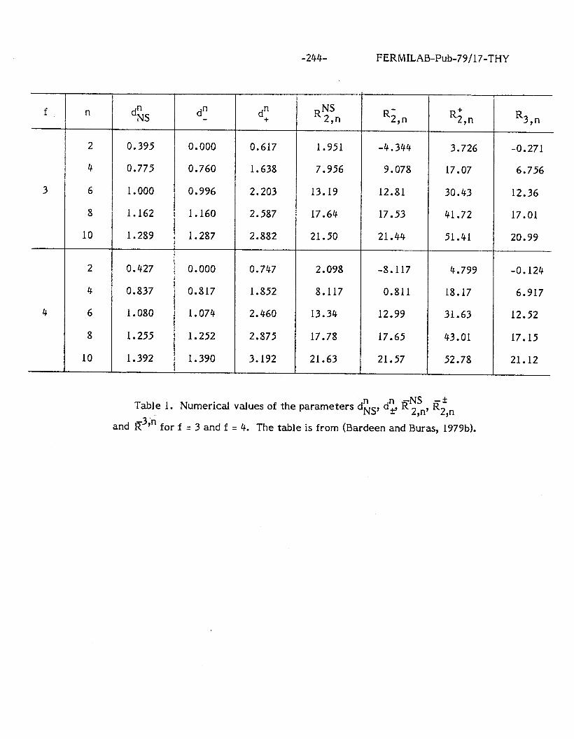
-244- FERMILAB-Pub-79/17-THY
n d” NS d” RNS 24 R2,n R;,n R3,n
2 0.395 0.000 0.617 1.951 -4.344 3.726 -0.271
4 0.775 0.760 1.638 7.956 9.078 17.07 6.756
6 1.000 0.996 2.203 13.19 12.81 30.43 12.36
8 1.162 1.160 2.587 17.64 17.53 41.72 17.01
10 1.289 1.287 2.882 21.50 21.44 51.41 20.99
2 0.427 0.000 0.747 2.098 -8.117 4.799 -0.124
4 0.837 0.817 1.852 8.117 0.811 18.17 6.917
6 1.080 1.074 2.460 13.34 12.99 31.63 12.52
8 1.255 1.252 2.875 17.78 17.65 43.01 17.15
10 1.392 1.390 3.192 21.63 21.57 52.78 21.12
-NS Table 1. Numerical values of the parameters dbs, d; R 2 n, 7 Ri n 9 and R3?” for f = 3 and f = 4. The table is from (Bardeen and Buras, 1979b).
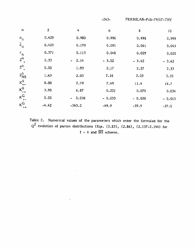
-245- FERMILAB-Pub-79/17-THY
n 2
a n 0.429
a n 0.429
E
Z:+
0.571
2.35
Z” 0.00
Z”NS 1.65
K$
K;-
0.00
Ki+
5.90
Kd-
0.00
-+ -4.42
4 6 8 10
0.980 0.996 0.998 0.999
0.170 0.091 0.061 0.045
0.113 0.048 0.029 0.020
- 2.14 - 3.02 - 3.42 - 3.62
1.95 2.17 2.27 2.35
2.05 2.16 2.25 2.33
2.79 7.49 11.4 14.7
6.87 0.221 0.070 0.034
- 0.056 - 0.033 - 0.020 - 0.013
-343.0 -49.9 -39.9 -37.0
Table 2. Numerical values of the parameters which enter the formulae for the Q2 evolution of parton distributions (Eqs. (2.85), (2.86), (2.137-2.144) for
f = 4 and MS scheme.
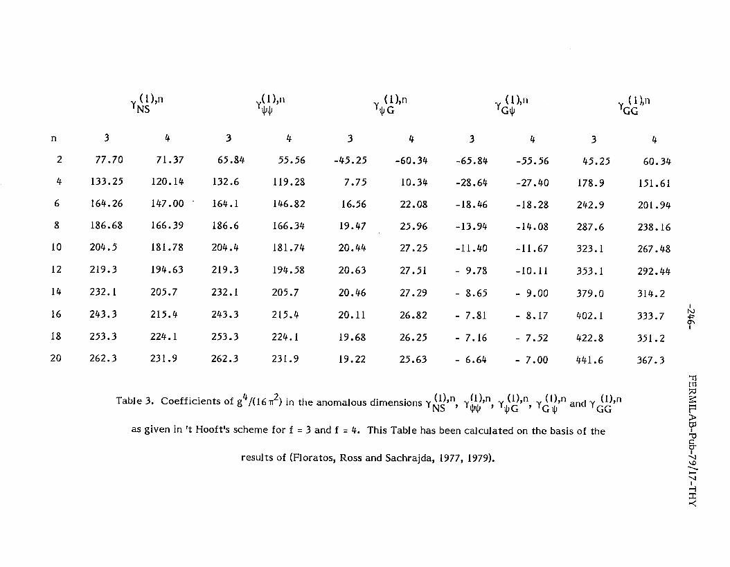
n 3 4 3 4
2 77.70 71.37 65.84 55.56
4 133.25 120.14 132.6 119.28
6 164.26 147.00 164.1 146.82
8 186.68 166.39 186.6 166.34
10 204.5 181.78 204.4 181.74
12 219.3 194.63 219.3 194.58
14 232.1 205.7 232.1 205.7
16 243.3 215.4 243.3 215.4
18 253.3 224.1 253.3 224.1
20 262.3 231 .v 262.3 231 .Y
( 1 ),Il yJJ9
(l),n hJc
3 4
-45.25 -60.34
7.75 10.34
16.56 22.08
19.47 25.96
20.44 27.25
20.63 27.51
20.46 27.29
20.11 26.82
19.68 26.25
19.22 25.63
3 4
-65.84 -55.56
-28.64 -27.40
-18.46 -18.28
-13.94 -14.08
-11.40 -11.67
- 9.78 -10.11
- 8.65 - 9.00
- 7.81 - 8.17
- 7.16 - 7.52
- 6.64 - 7.00
3 4
45.25 60.34
178.9 151.61
242.9 201.94
287.6 238.16
323.1 267.48
353.1 292.44
379.0 314.2
402.1 333.7 $ I
422.8 351.2
441.6 367.3
ts! Table 3. Coefficients of g4/(l 6 a21 in the anomalous dimensions yf$isn, ~4~’ (l) 7 y ‘2”
, ydl),n (lb and Y GG II, 4J
as given in ‘t Hooft’s scheme for f = 3 and f = 4. This Table has been calculated on the basis of the
results of (Floratos, Ross and Sachrajda, 1977, 1979).
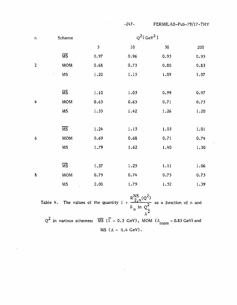
-247- FERMILAB-Pub-79/17-THY
n Scheme
MS
MOM
MS
Q2 [ GeV2 ’
5 10
0.97 0.96
0.68 0.73
1.20 1.15
J
50
0.95
0.80
1.09
200
0.95
0.83
1.07
MS 1.10 1.05 0.99 0.97
MOM 0.63 0.65 0.71 0.75
MS 1.53 1.42 1.26 1.20
MS 1.24 1.15 1.05 1.01
MOM 0.69 0.68 0.71 0.74
MS 1.79 1.62 1.40 1.30
MS 1.37 1.25 1.11 1.06
8 MOM 0.79 0.74 0.73 0.75
MS 2.00 1.79 1.52 1.39
Table 4. The values of the quantity 1 + R;~,(Q~)
B, In 2 as a function of n and
A2 Q2 in various schemes: MS (R = 0.5 GeV) , MOM (hmom = 0.85 GeV) and
MS (A = 0.4 GeV).
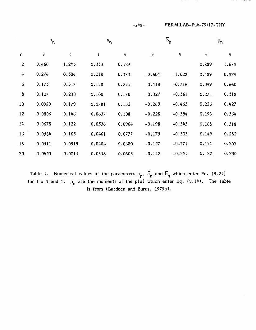
-248- FERMILAB-Pub-79/17-THY
n 3 4
2 0.660 1.245
4 0.276 0.504
6 0.175 0.317
8 0.127 0.230
10 0.0989 0.179
12 0.0806 0.146
14 0.0678 0.122
16 0.0584 0.105
18 0.0511 0.0919
20 0.0453 0.0815
a n
0.353
0.218
0.138
0.100
0.0781
0.0637
0.0536
0.0461
0.0404
0.0358
2 n
4
0.529
0.373 -0.604 -1.028
0.235 -0.418 -0.716
0.170 -0.327 -0.561
0.132 -0.269 -0.463
0.108 -0.228 -0.394
0.0904 -0.198 -0.343
0.0777 -0.175 -0.303
0.0680 -0.157 -0.271
0.0603 -0.142 -0.245
3 4 3 4
0.889 1.679
0.489 0.924
0.349 0.660
0.274 0.518
0.226 0.427
0.193 0.364
0.168 0.318
0.149 0.282
0.134 0.253
0.122 0.230
Table 5. Numerical values of the parameters an, a, ana F,, which enter Eq. (9.25)
5-l pn
for f = 3 and 4. p, are the moments of the p(x) which enter Eq. (9.14). The Table is from (Bardeen and Buras, 1979a).
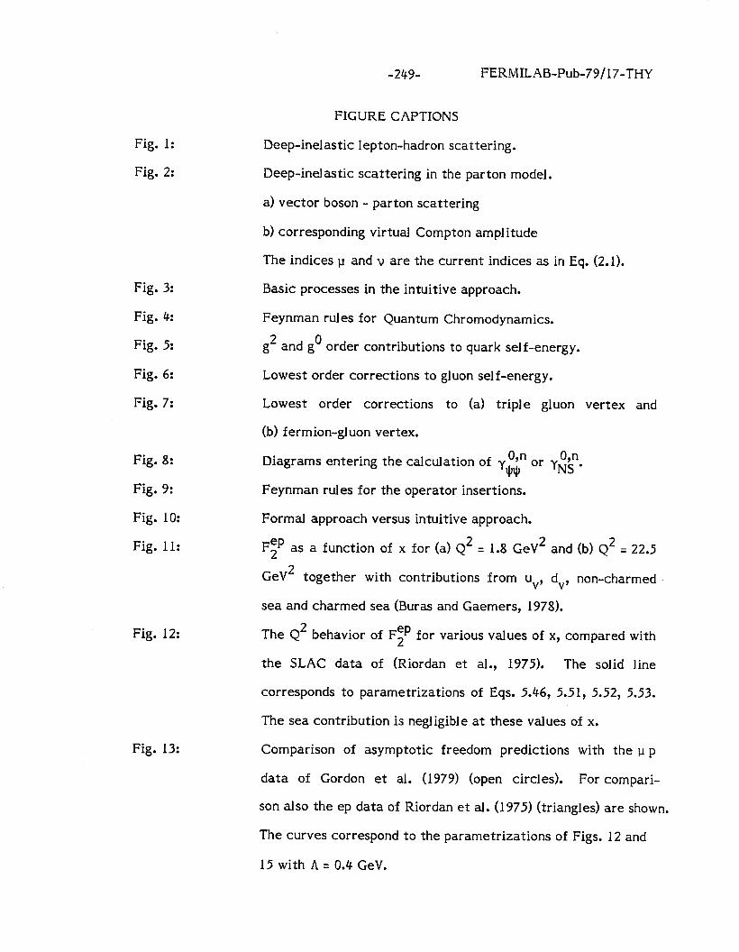
-249- FERMILAB-Pub-79/17-THY
Fig. 1:
Fig. 2:
Fig. 3:
Fig. 4:
Fig. 5:
Fig. 6:
Fig. 7:
Fig. 8:
Fig. 9:
Fig. 10:
Fig. 11:
Fig. 12:
Fig. 13:
FIGURE CAPTIONS
Deep-inelastic lepton-hadron scattering.
Deep-inelastic scattering in the parton model.
a) vector boson - parton scattering
b) corresponding virtual Compton amplitude
The indices p and v are the current indices as in Eq. (2.1).
Basic processes in the intuitive approach.
Feynman rules for Quantum Chromodynamics.
g2 and go order contributions to quark self-energy.
Lowest order corrections to gluon self-energy.
Lowest order corrections to (a) triple gluon vertex and
(b) fermion-gluon vertex.
Diagrams entering the calculation of y lil;”
O,* Or YNS l
Feynman rules for the operator insertions.
Formal approach versus intuitive approach.
Fzp as a function of x for (a) Q2 = 1.8 GeV2 and (b) Q2 = 22.5
GeV2 together with contributions from uv, dv, non-charmed
sea and charmed sea (Buras and Gaemers, 1978).
The Q2 behavior of Fzp for various values of x, compared with
the SLAC data of (Riordan et al., 1975). The solid line
corresponds to parametrizations of Eqs. 5.46, 5.51, 5.52, 5.53.
The sea contribution is negligible at these values of x.
Comparison of asymptotic freedom predictions with the p p
data of Gordon et al. (1979) (open circles). For compari-
son also the ep data of Riordan et al. (1975) (triangles) are shown.
The curves correspond to the parametrizations of Figs. 12 and
15 with A = 0.4 GeV.
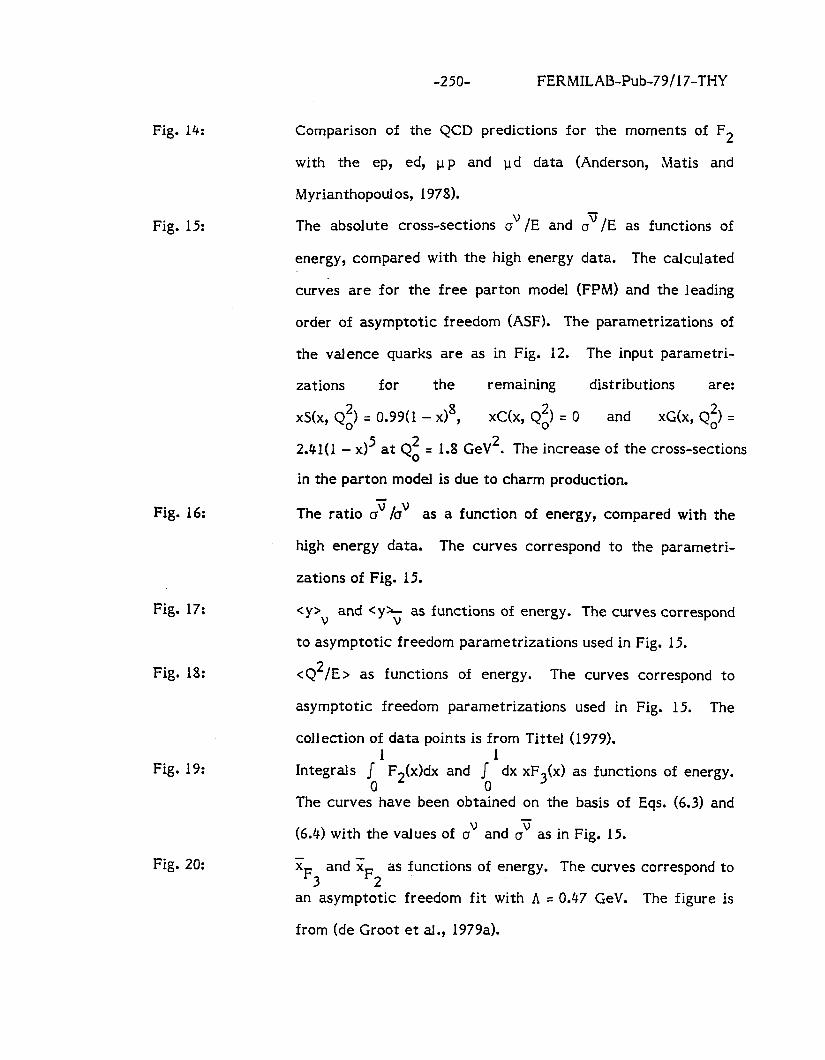
-250- FERMILAB-Pub-79/17-THY
Fig. 14:
Fig. 15:
Fig. 16:
Fig. 17:
Fig. 18:
Fig. 19:
Fig. 20:
Comparison of the QCD predictions for the moments of F2
with the ep, ed, u p and pd data (Anderson, Matis and
Myrianthopoulos, 1978).
The absolute cross-sections a’ /E and crv/E as functions of
energy, compared with the high energy data. The calculated
curves are for the free parton model (FPM) and the leading
order of asymptotic freedom (ASF). The parametrizations of
the valence quarks are as in Fig. 12. The input parametri-
zations for the remaining distributions are:
xS(x, Q;) = 0.99(1 - x18, xC(x, Q;) = 0 and xG(x, Q;) =
2.41(1 - xJ5 at Qz = 1.8 GeV2. The increase of the cross-sections
in the parton model is due to charm production.
The ratio o’/ov as a function of energy, compared with the
high energy data. The curves correspond to the parametri-
zations of Fig. 15.
<Y>~ and <yk as functions of energy. The curves correspond
to asymptotic freedom parametrizations used in Fig. 15.
<Q2/E> as functions of energy. The curves correspond to
asymptotic freedom parametrizations used in Fig. 15. The
collection of data points is from Tittel (1979). 1 1
Integrals I F (x)dx and I dx xF3(x) as functions of energy. 0 2 0
The curves have been obtained on the basis of Eqs. (6.3) and
(6.4) with the values of ov and d as in Fig. 15.
x F3
and x F2
as functions of energy. The curves correspond to
an asymptotic freedom fit with A = 0.47 GeV. The figure is
from (de Groot et al., 1979a).
-251- FERMILAB-Pub-79/17-THY
Fig. 21:
Fig. 22:
Fig. 23:
Fig. 24:
Fig. 25:
Fig. 26:
Fig. 27:
Fig. 28:
Fig. 29:
Fig. 30:
F2(x, Q’) as measured by the CDHS group (de Groot et al.,
1979a) (black points) compared with the leading order asymp-
totic freedom predictions for A = 0.47 GeV. The open points
are from SLAC. The figure is from (de Groot et al., 1979a).
log Mi versus log Mj plots as obtained by CDHS and
BEBC/GGM. The figure is from (de Groot et al., 1979a).
The measured slopes as defined by the plots of Fig. 22. The
straight horizontal lines are the predictions of vector gluon
and scalar gluon theories.
(lb Examples of diagrams which enter the calculation of y NS .
Examples of g4 order contributions to quark self energy.
Diagrams entering the calculation of Tk n (2)9NS of Eq. (7.31). ?
Order g2 deviations from the Gross-Llewellyn-Smith and
Bjorken sum rules. The dashed lines (---I are parton model
predictions. The solid ( -1 lines follow from Eqs. (2.99) and
(2.100). The f’ igure is from (Bardeen et al., 1978).
Nachtmann moments of xF3(x, Q2) 5. Q2. The data are from
(Bossetti et al., 1978). The solid lines represent the MS and MS
schemes.
Experimental An values obtained by Duke and Roberts (1979)
using the data of BEBC (open box), CDHS (open diamond) and
the entire SLAC data.
The effective AF)(Q2) (-) as defined by Eqs. (7.68) and (7.69)
as functions of n for various values of Q2 and x= 0.5 GeV. For
(2) comparison the An as defined by Eq. (7.63) is plotted as
functions of n for K= 0.35 GeV.
-252- FERMILAB-Pub-79/17-THY
Fig. 31:
Fig. 32:
Fig. 33:
Fig. 34: Diagrams entering the calculation of Tk n (2)yG of Eq. (8.55). Y Fig. 35: Size of the explicit second order corrections Ii 2,n(z) in the MS
Fig. 36:
Fig. 37:
Fig. 38:
Fig.39:
The effective coupling constants Z(Q2) as extracted from the
BEBC data for the leading order (L.O.), MS scheme, m scheme
and momentum subtraction scheme MOM.
Examples of the diagrams which enter the calculation of the
two-loop anomalous dimension matrix y
y tJ,“(e, f) and y$,“(g, h).
($“(a, b), y$,*(c, d),
Examples of the diagrams which enter the calculation of the
anomalous dimension of the gluon field in order g4.
scheme for f = 4.
Diagrams contributing to photon(w )-quark(+) scattering
to order g2. The empty (“bare,,) blob stands for the “bare,, (Q2
independent) quark distribution in the proton. m denotes
gi uon.
The ratio R as given by Eq. (9.9) as a function of $-2- Q for two
values of A. The heavy lepton contribution (AR = 1) has been
added. The parton model prediction is R = 4.3.
The process e+e- -c hadron + e+e-:
a) The dominant two-photon contribution
b) Vector dominance contribution to the photon-photon scat-
tering
c) Contributions to photon-photon scattering in which the
photon behaves like a point-like particle (parton model
diagram).
Typical diagrams contributing to the mixing between hadronic
operators and the photon operator a) K ‘,n ,,, b) K(d),” c) Kt),*,
-253- FERMILAB-Pub-79/17-THY
Fig. 40:
Fig. 41: Illustration of the r.h.s. of Eq. (9.29). The sum runs over
quarks and gluons.
Fig. 42: Illustration of the r.h.s. of Eq. (9.36). The sum runs over
Fig. 43:
Fig. 44:
Fig. 45:
Fig. 46:
Moments of the photon structure function in units of c1 2 as
predicted by the parton model (a), asymptotic freedom in the
leading order (b), and asymptotic freedom with higher order
corrections (c, d, e). For comparison the same value of A for
all cases has been chosen.
quarks and gluons.
Basic processes responsible for the Q2 evolution of the frag-
mentation functions.
Diagrams contributing to quark (b-1 production in
e+e- + h + anything to order g2. The empty (“bare”) blob
stands for the “bare” Q2 independent quark fragmentation
functions. LUW denotes gluons.
Illustration of the r.h.s. of Eq. (9.56). The sums run over
quarks and gluons.
Illustration of the r.h.s. of Eq. (9.57). The sums run over
quarks and gluons.
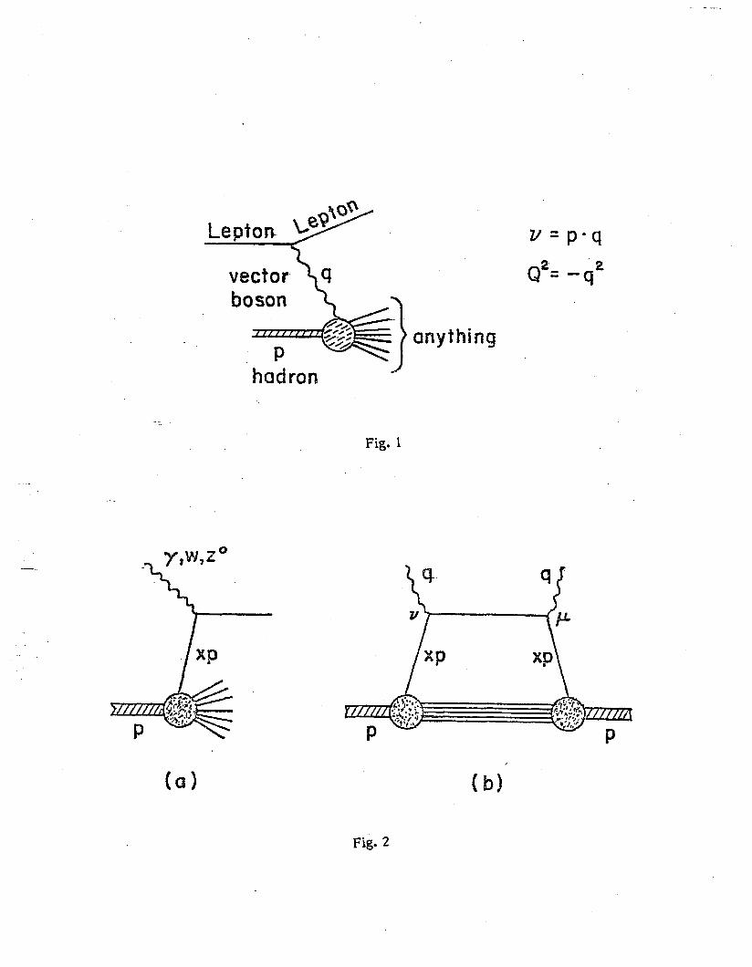
anything
hadron
- . .
Fig. I
Y = p-4
Q”= --$
Fig. 2
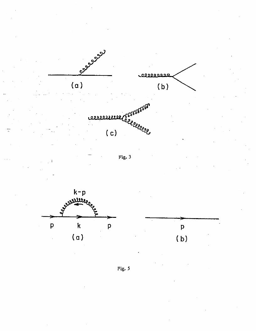
- . .
( 1 cl -,
- -.
Fig. 3
-
k P
Fig. 5
(W
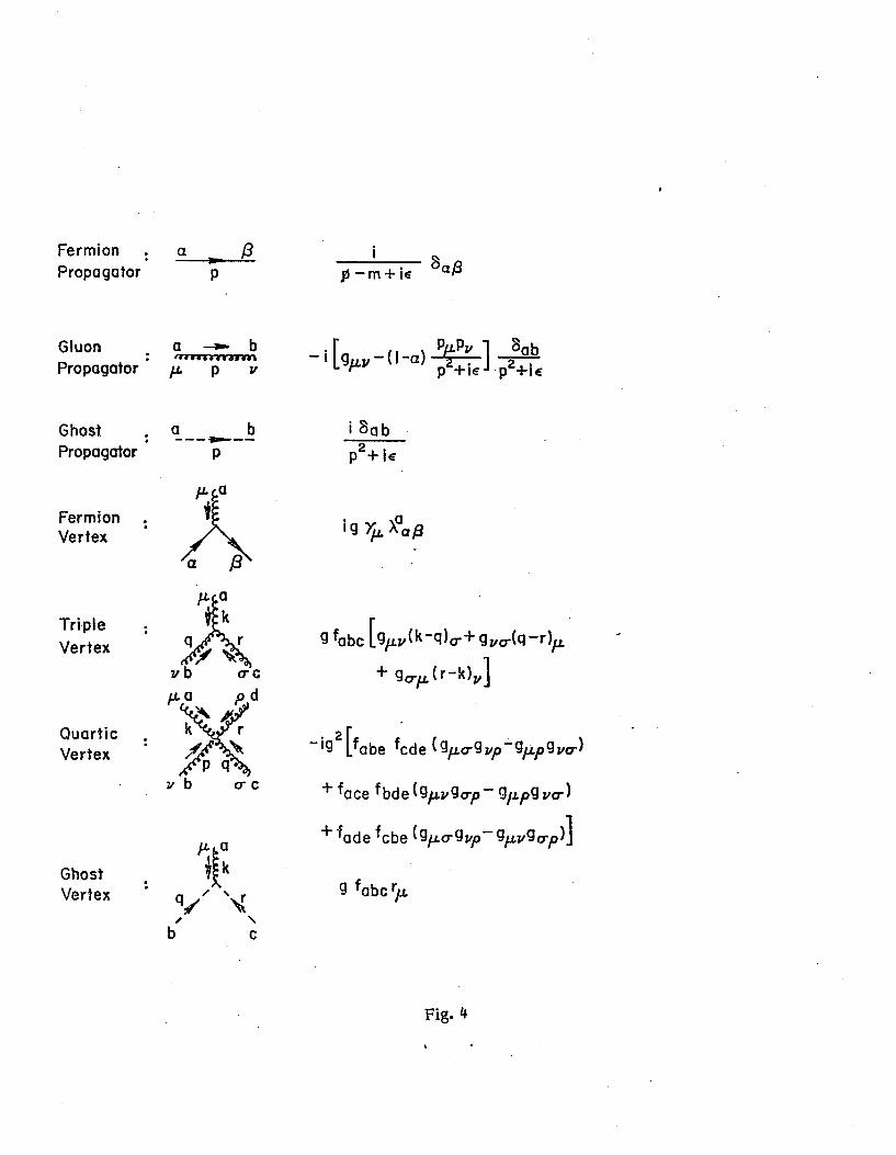
Fermion : u _ P Propagator P
Gluon a b 4
Propagator ’ p p v -
Ghost Propagator ’
a b w-- --- p
Fermion - Vertex
. .
i Sob p*+ ir
Tri,ple : Vertex g,.&-d& g&r+
+ gcrtL (r-k),]
Quartic : Vertex
-ig2 f I: abe fcde gp(rgv,o-gtLpgv=) (
vb O-C +face fbde(gpv9~p-!JppSvcr)
+fade fcbe (gpogvp-gpvgdp )I Ghost Vertex ’ 9 fabcrp
Fig. 4
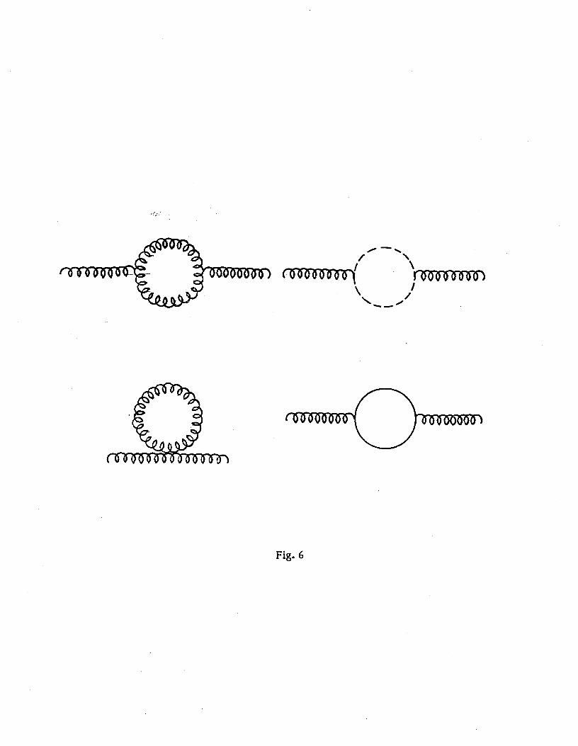
Fig. 6
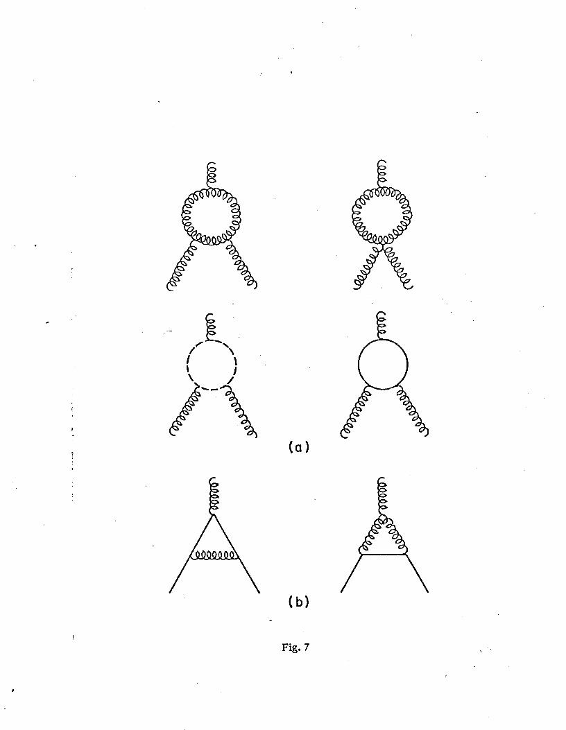
.
h
b)
Fig. 7
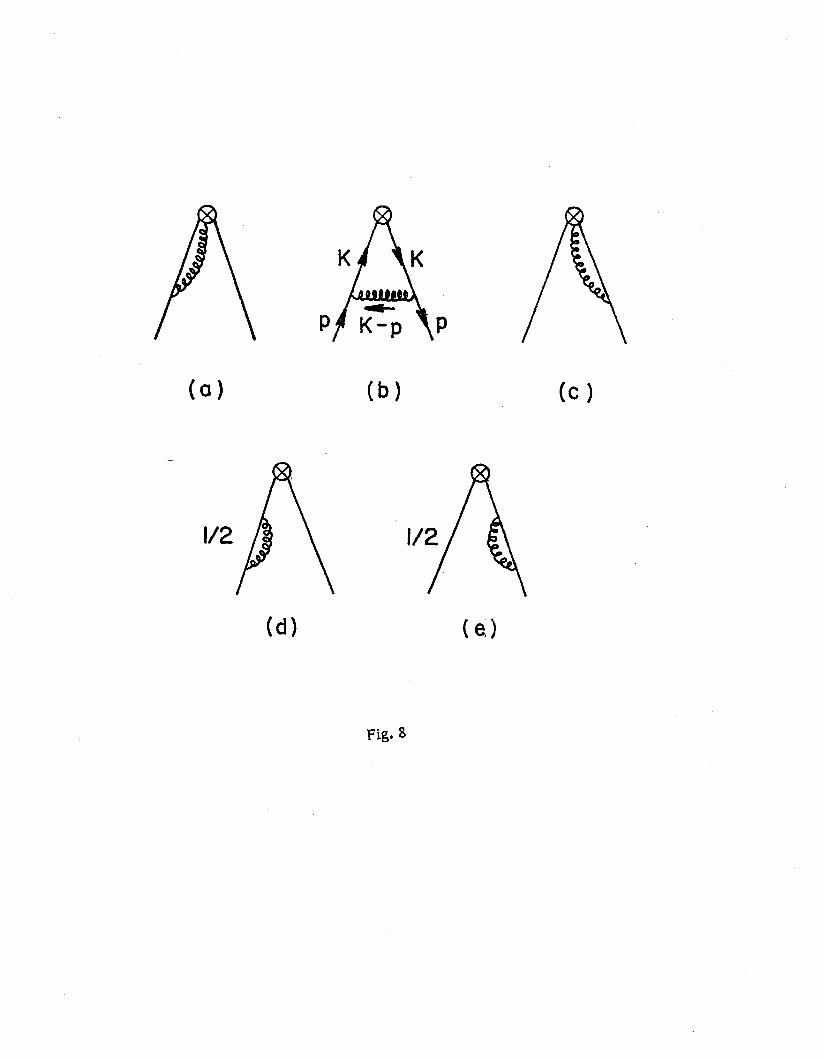
A ( 1 a (b) (c 1
- ,,*/I// ,,A
Fig. 8
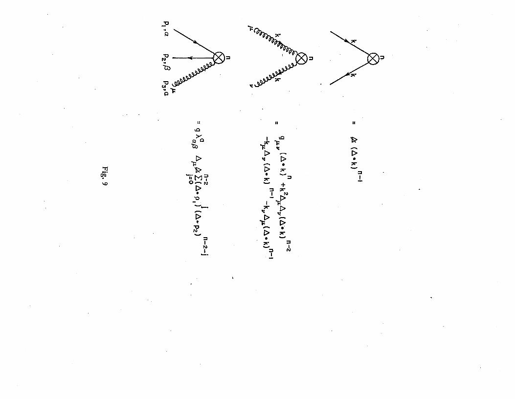
II II
.
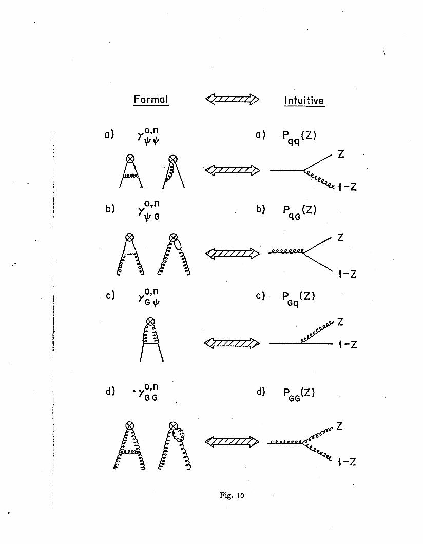
, ‘, \
I !
i
i !
. .
Formal
A R
cl an yw
A d) l y:G” .
Intuitive
<
z ‘-
f-Z
‘&)
c). pGq(z)
4 p,,(z)
I
Fig. 10
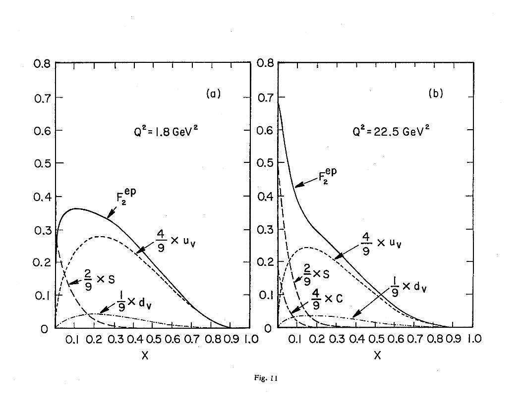
0.8 I I I I I I I I I 0.8 I I I I I I I I I
0.7 (4 0.7 (b) 0.6 Cl’= 1.8 GeV’ 0.6 Q2= 22.5 GeV2
0.5
0.4
0.3
0.2
0. I
0
Fep
A
2 I!
0.5
0.4
0.3
0.2
0.1
0
\ dF eP
2
0.1 0.2 0.3 0.405 0.6 0.7 0.80.9 I.0 X
0.1 0.2 0.3 0.4 0.5 0.6 0.7 0.8 0.9 I .O X
Fig. 11
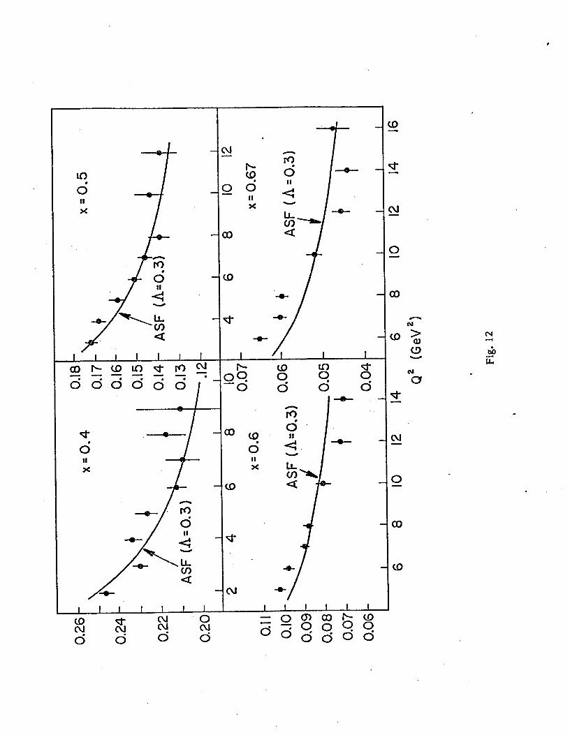
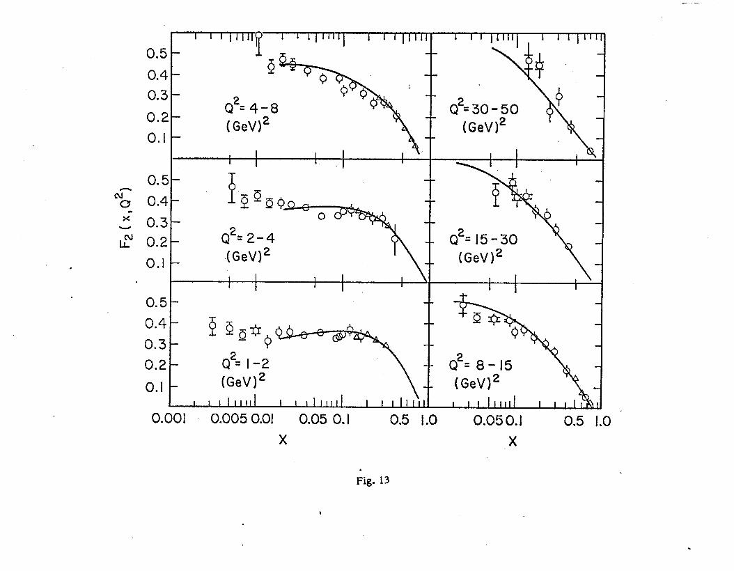
Q2= 4-8 ( GeV12
0.5 ’ 0.4
0.3 0.2
0.1 1
4 ‘Q P P
Q2= 2-4 (GeW2
Q2z I-2
(GeV)*
I I I llll I II
.
. 4
*‘Y
If
Q2=30-50 0
tGeV)*
I I ,\
x ’
E
Q2= 15-30 (GeV)*
(GeV)’
. Fig. 13
.
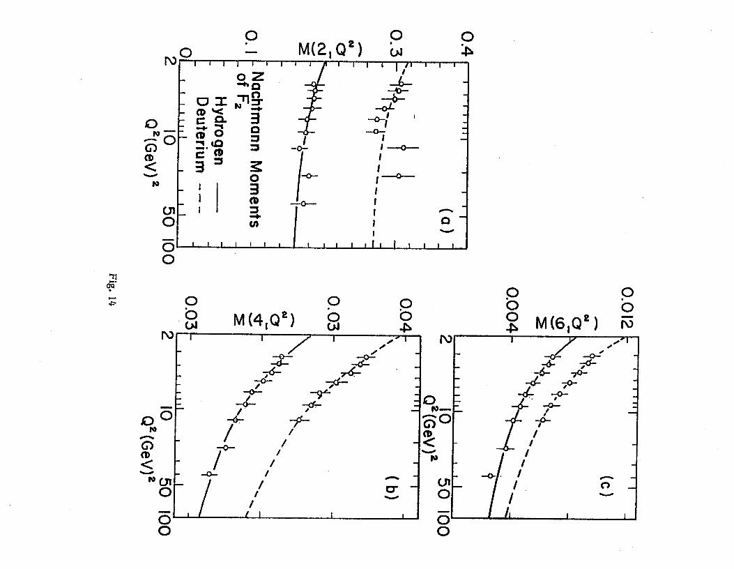
0
2 ? 0
M(4,Q’) 8 0
NN 4
l zs
l 0
p M(6,cY) fG 1
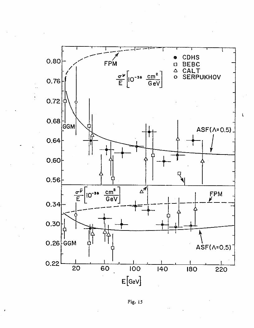
f I I I’ I I I
-I
0.80- //’
7’
e CDWS q BEBC a CALT 0 SERPUKWOV i
ASF( A= 0.5) 1 0.64
0.56t
3 -38 cm2 I
d GeV
--I---?--
0.221 i. I I I I I I I I I I I I 60 100 140 180 220
EEG VI e
Fig. 15
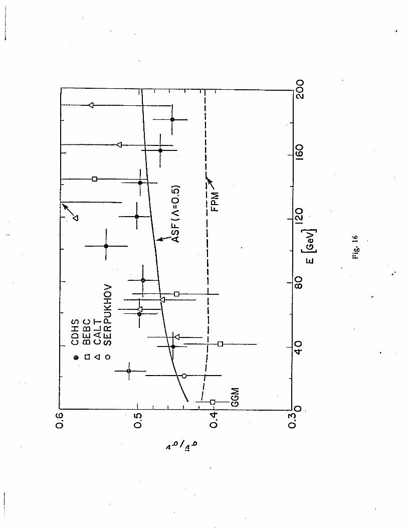
b
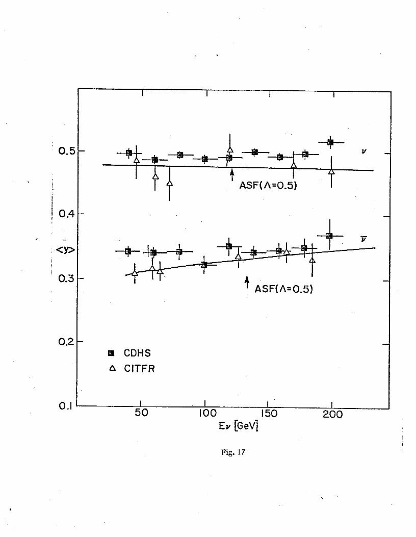
.
0.2
0.1
m CDHS a CITFR
I 50
I I I 100 150 200
EZJ [GeV]
Fig. 17
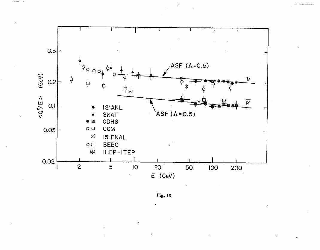
0.5
0.05
I I I I I I I
I
i-
@ q CDHS 00 GGM
X 15’FNAL 00 BEBC
W IHEP- ITEP
0.02 - I
I I I I I I I
2 5 IO 20 E (GeV)
50 100 200
Fig. 18
. .
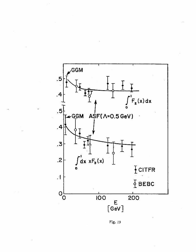
w
.5
.4
.3
.2
: I
I 0
~GiM ASFCA=0.5 GeV) -
0 i CITFR
I
P BEBC
OL 0
Fig. 19
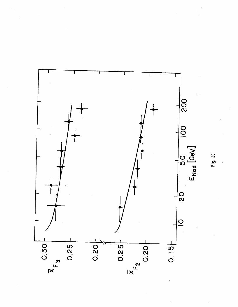
I I I I I
I I I \, I -bx I n L _- _-
d
.
>
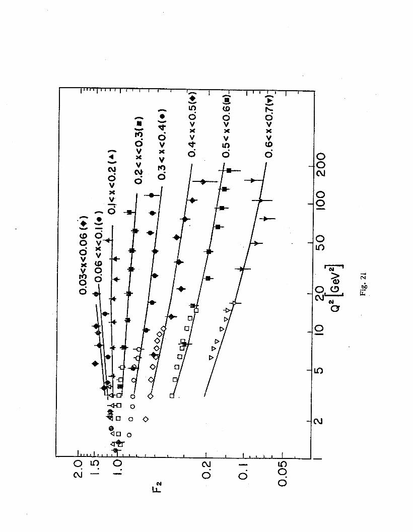
D
DD
1 D 10
N
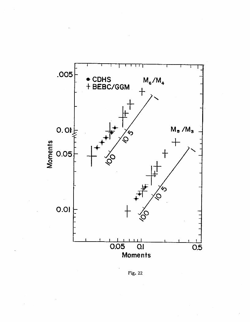
.005
0.01
I I I I ’ ’ “I I I
m
l CDHS
-I- BEBWGGM 1 Me/M,,
I I I I f IllI I t t I 0.05 0.1 0.5
MOlllWltS
Fig. 22
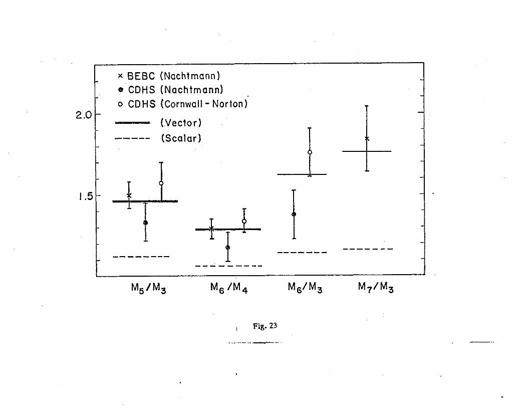
2.0
I .5 I-
x BEBC (Nachtmann) *‘CDHS (N.achtmann) 0 CDHS (Cornwall - Norton)’ T
-. (.Vecto ----- (Scala
-4-J- r
f) r)
+4- i-
?
-m----m --e---e
-------a
1
-w------w
Md”3 b/M,
.
I Fig. 23
-._- --a---..
.
--.
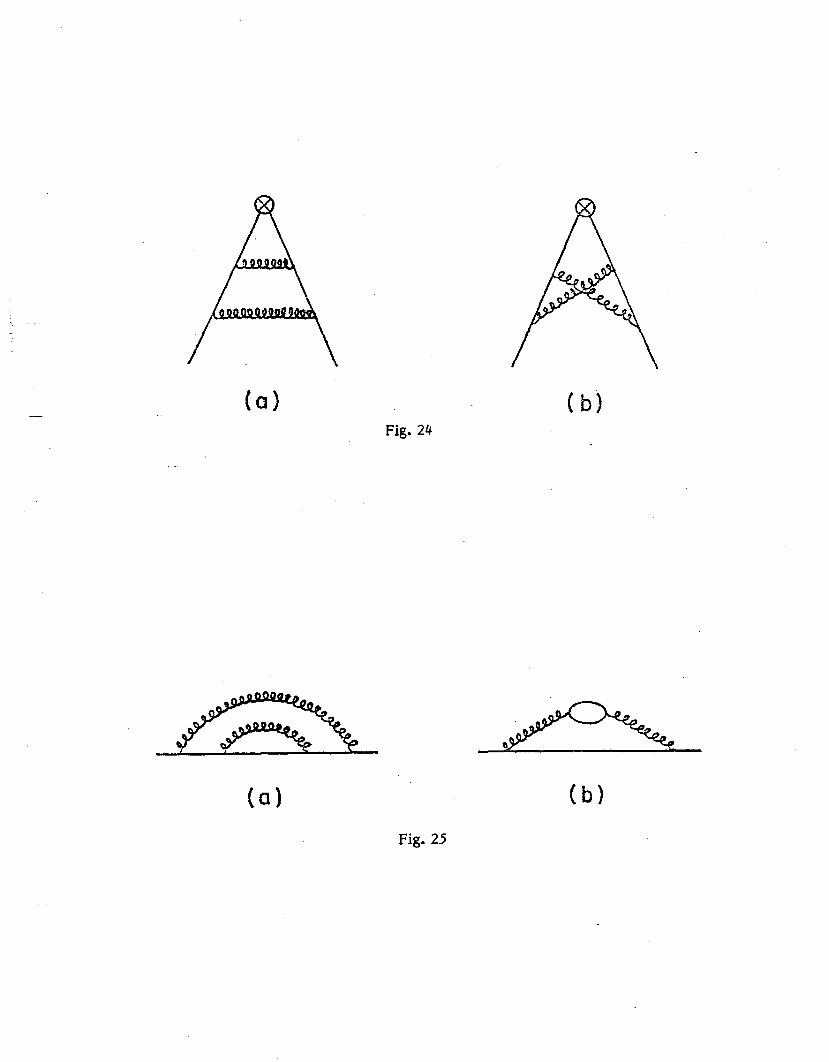
( > cl Fig. 24
( 1 Q
(b)
(b) Fig. 25
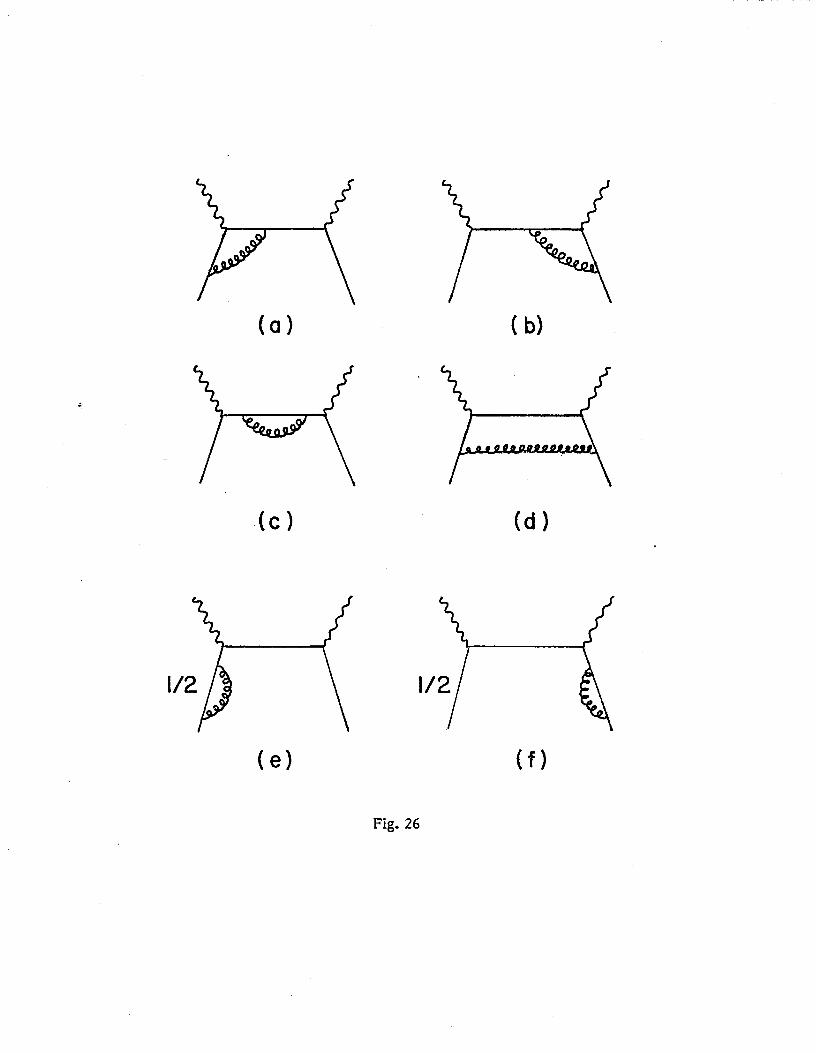
( 1 a (b)
W (f)
Fig. 26
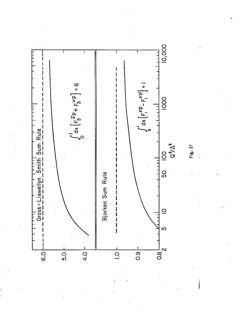
8 0
e-
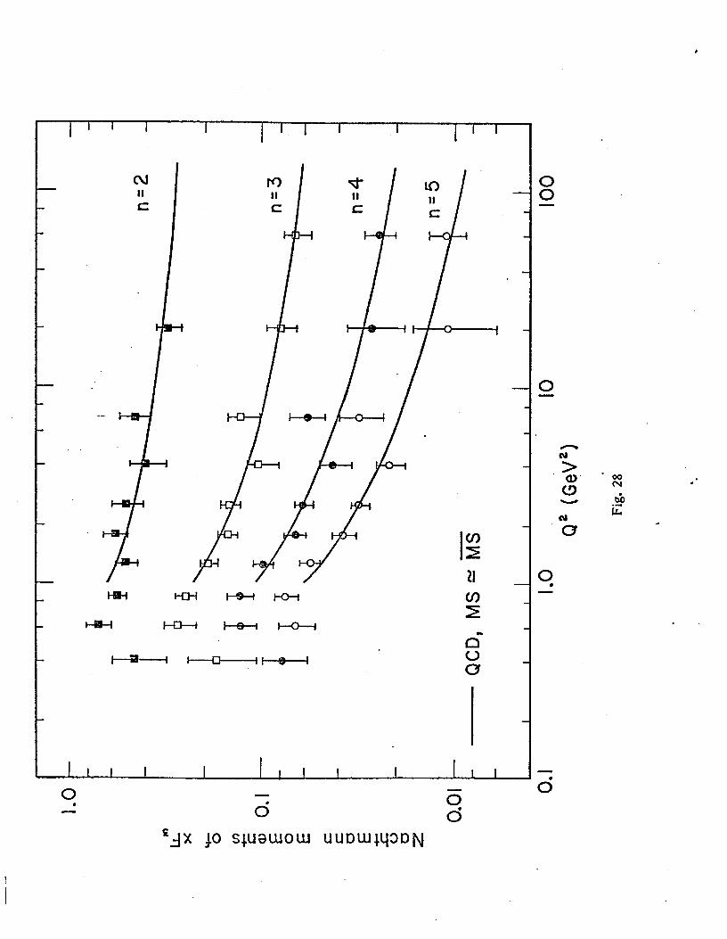
,
-
-
I I
cu II c
HH t-@+l-cH
-t-e-i-
t-al -l--e--i
s -
0
2 ‘% (3 . - OJ
iz” :
.
- 6
‘AX JO S&K3UlOlU UUDUl+YZDN
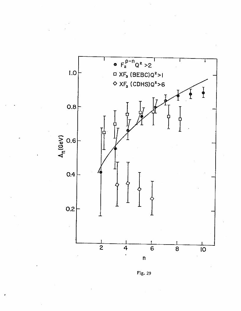
.
I.(
0.t
‘0.2
3-
3-
3-
c-
), .
L
I @ F,P-“Q2 >2’ ’
I
q XF, (BEBC)Q*>I
I 1 I I I r) A A L Lt b tJ IO
. n
Fig. 29
,
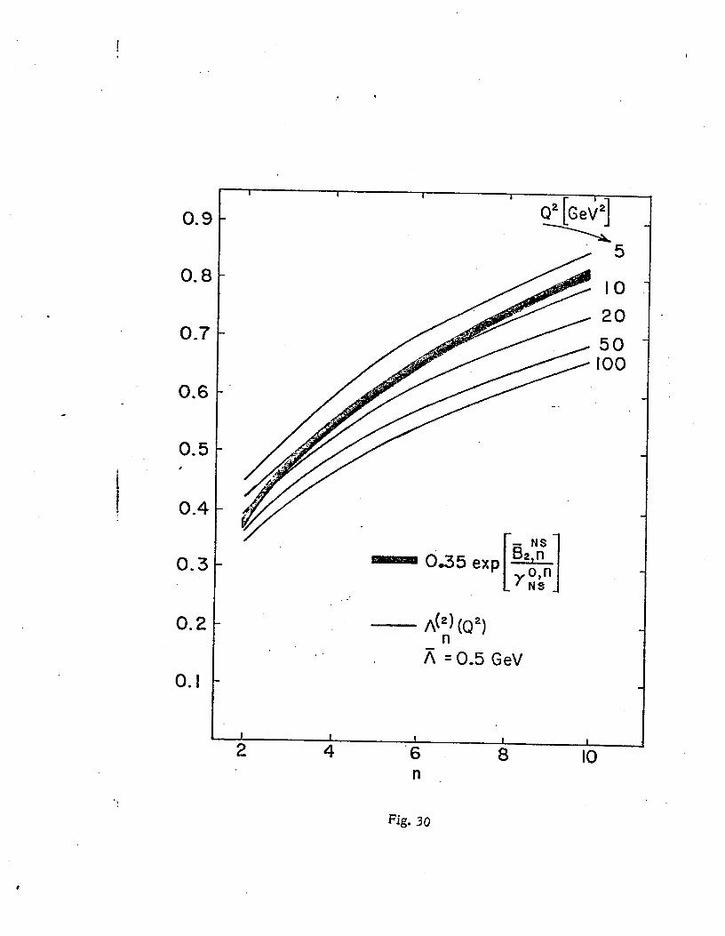
. .
0.7
0.6
0.3
0.2 A(‘,’ (Q')
0. I
0.35 exp 82,Nns [ I on ytdii
A = 0.5 GeV
t I I I 2 4
1 ‘6 8 IO n
Fig. 30
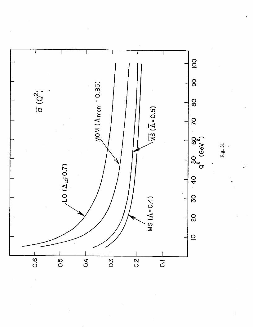
‘9 0 d
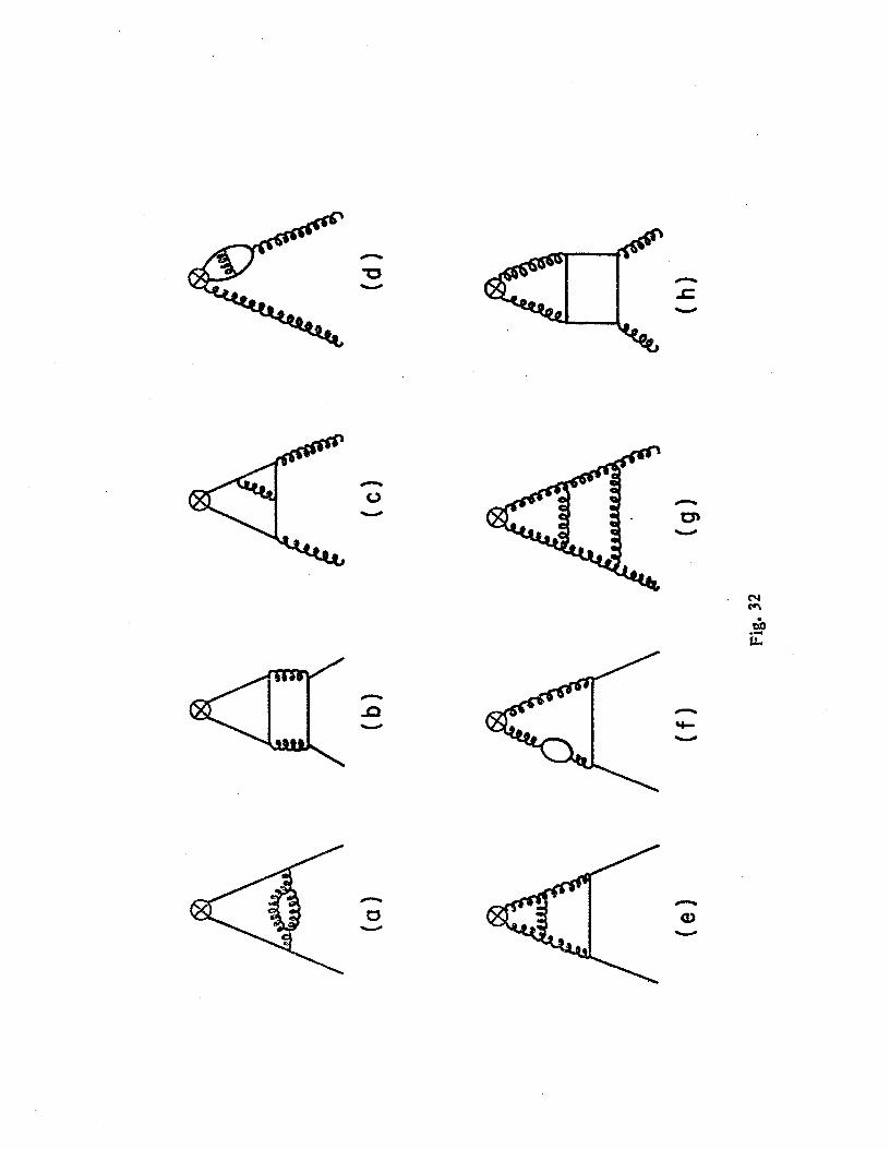
- -a -
- 0
-
<-
n
- m
u
-
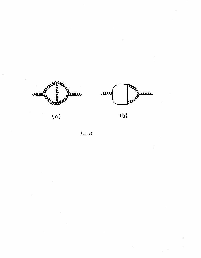
(a) (b)
Fig. 33
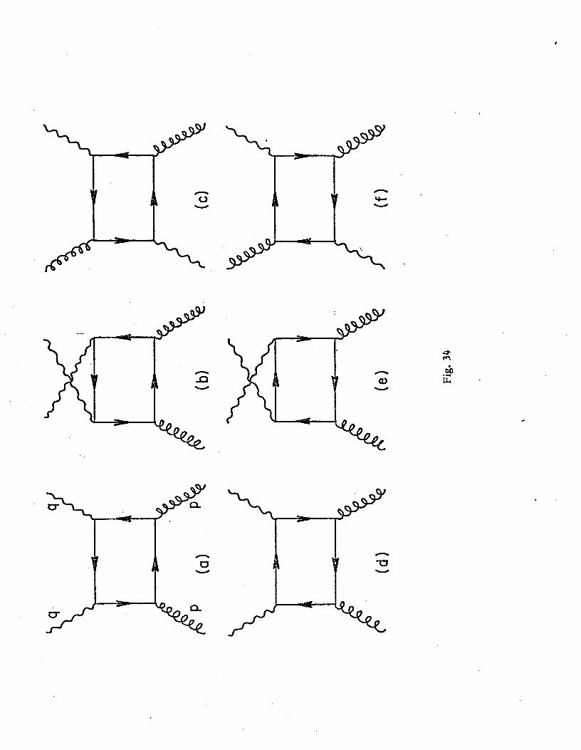
.
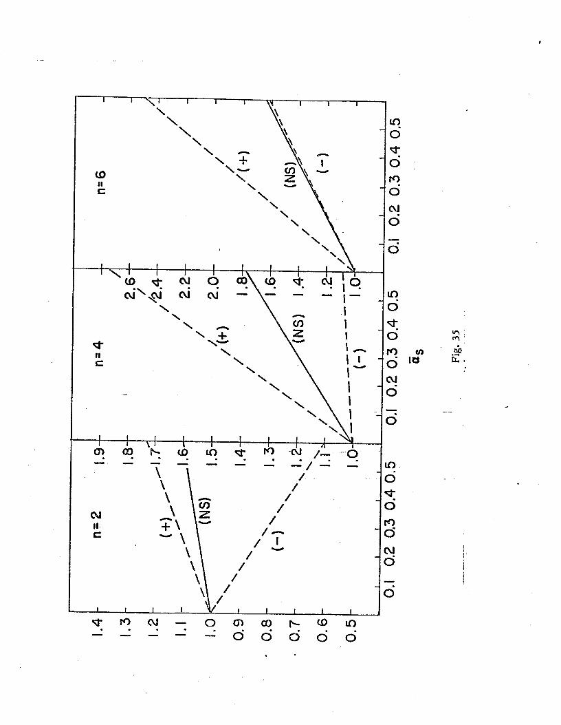
-\ \
\ \
\
I I
\ \ I \ I
\ \ \ \ G
T\ t -\
\ \
N 5
3 --
0. j .- j: 3
3
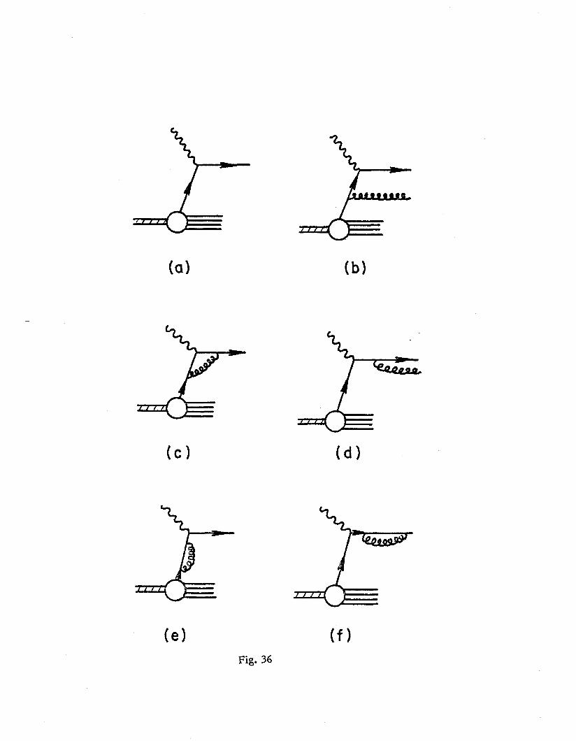
( 1 a
(cl
W
(d)
(4 (0 Fig. 36
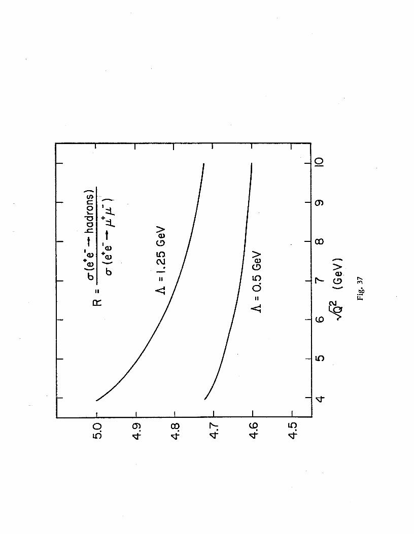
1 i I 7
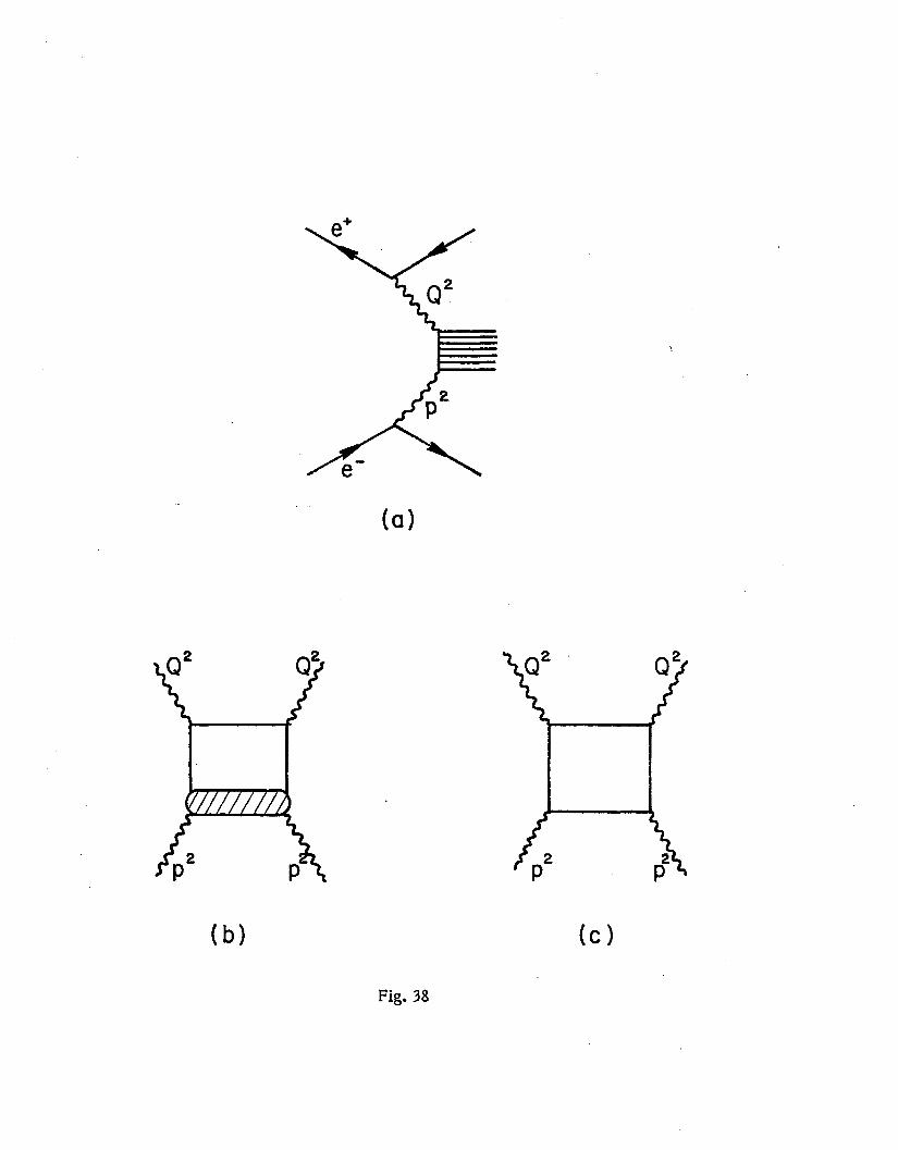
e+
Y Q2
P2 A e’
Fig. 38
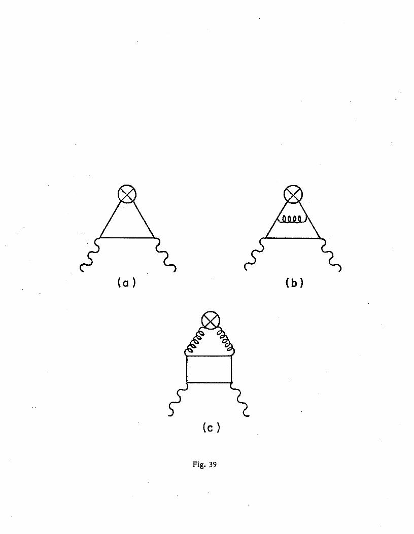
-
(b)
Fig. 39
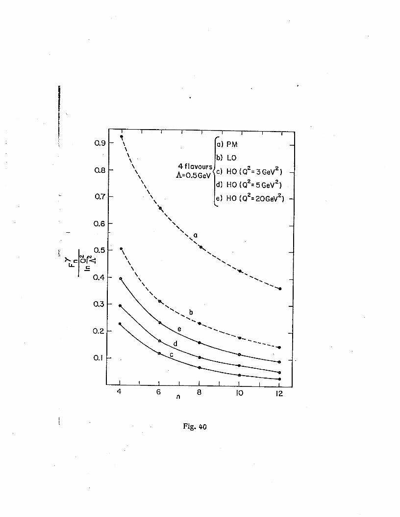
0.5
-. 0.1
0.6 -
0.3
I I I I I I I I t
I
- \ \
\ \ ‘t
HO (Q2= 20GeV2)
\ \ \ \ \
. 0
I I I I I I I I I 4
’ n 8 IO 12
Fig. 40
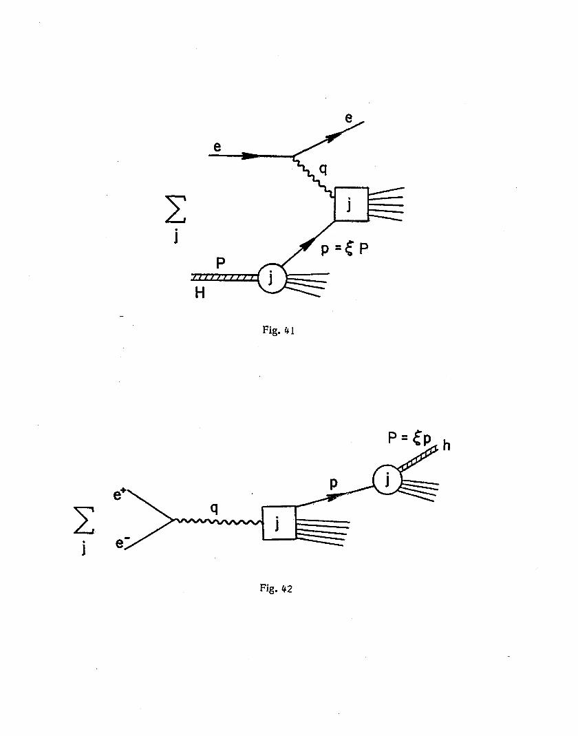
c i
c j
Fig. 41
Fig. 42
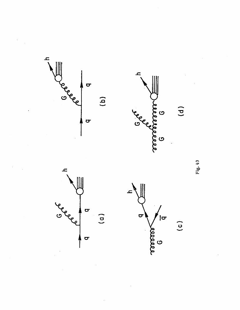
-
u -
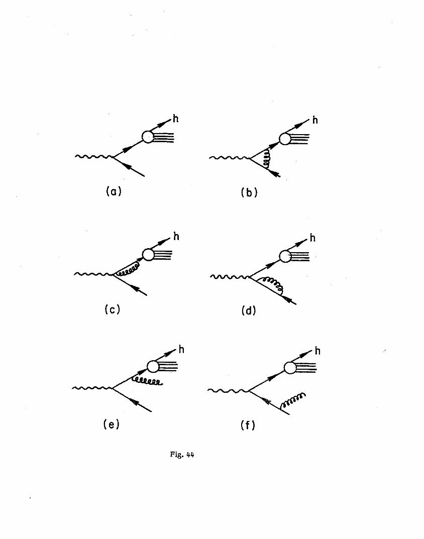
(a) (b)
(cl
h
(d)
Fig. 44
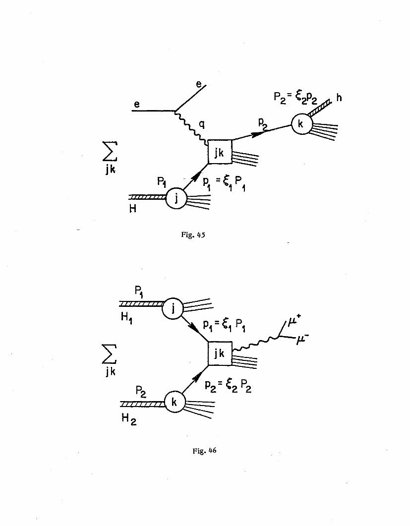
e,
c jk
c jk
e
Jjk &
Fig. 45
Fig. 46