HAL Id: hal-02173458https://hal.archives-ouvertes.fr/hal-02173458

Submitted on 15 Nov 2021

HAL is a multi-disciplinary open accessarchive for the deposit and dissemination of sci-entific research documents, whether they are pub-lished or not. The documents may come fromteaching and research institutions in France orabroad, or from public or private research centers.

L’archive ouverte pluridisciplinaire HAL, estdestinée au dépôt et à la diffusion de documentsscientifiques de niveau recherche, publiés ou non,émanant des établissements d’enseignement et derecherche français ou étrangers, des laboratoirespublics ou privés.

Distributed under a Creative Commons Attribution - NonCommercial| 4.0 InternationalLicense

Finite element analysis of composite forming atmacroscopic and mesoscopic scale

Philippe Boisse, Naïm Naouar, Adrien Charmetant

To cite this version:Philippe Boisse, Naïm Naouar, Adrien Charmetant. Finite element analysis of composite formingat macroscopic and mesoscopic scale. Advances in Composites Manufacturing and Process Design,Elsevier, pp.297-315, 2015, 978-1-78242-307-2. �10.1016/B978-1-78242-307-2.00014-2�. �hal-02173458�

1

Finite element analysis of composite forming at macroscopic and

mesoscopic scale

Philippe Boisse, Naim Naouar, Adrien Charmetant,

Université de Lyon, INSA-Lyon, LaMCoS, F-69621 Lyon, France

Abstract

F.E. analyses of composite reinforcement forming are presented at macroscopic and

mesoscopic scale. Simulations of 3D interlock fabric deformations are based on a hyperelastic

model. The strain energy model uses the strain invariants representative to independent

deformation modes of the interlock fabric. In a second part, a simulation at mescoscale of the

deformation of a textile composite reinforcement is presented. The F.E. model is obtained

from X-ray computed tomography of the fabric in order to be close to the real geometry. The

advantage of such an approach in comparison to the use of a textile geometrical modeler is

shown.

1 – Introduction.

R.T.M process produces high-performance composite parts by resin injection on a textile

reinforcement made of continuous fibres (Advani, 1994; Ruiz et al., 2011). This

reinforcement, called preform, is shaped before resin injection. Complex shapes, in particular

with double curvatures can be obtained by membrane deformations of the textile

reinforcement. In plane shear angle is the main strain that allows to reach double curved

shapes. Nevertheless all the shapes are not possible for a given reinforcement. Some defects

can appear during forming such as wrinkles, gaps between the yarns, fracture of yarns …To

avoid the costly development by try and error of these forming processes, the numerical

2

simulation can predict if the manufacturing process is possible and what are the conditions for

a good achievement.

Two families of methods exist for fibrous reinforcement forming (or draping): kinematic and

mechanical approaches. Kinematic models (fishnet algorithms) assume that the fibres are

inextensible and that the reinforcement is mapped onto the surface of the component/forming

tool by assuming that tow segments are able to freely shear at tow crossovers (Mark and

Taylor, 1956; Van Der Ween, 1991). The mechanical behavior of the reinforcement, the

exterior loads, sliding and friction on the tools are not taken into account. The main advantage

of these methods is the small CPU times needed. On the other hand wrinkles and the effects

of blank holders cannot be analyzed. The influence of the nature of the reinforcement cannot

be analyzed either. The present chapter concerns mechanical approaches. The forming process

is analyzed as a thermomechanical transformation of the composite submitted to

displacements and temperature of the tools. The simulation needs an efficient mechanical law

for the analyzed reinforcement or prepreg and an efficient finite element approach. The

analysis is performed at finite strain. The mechanical behavior of the reinforcements is

strongly influenced by its fibrous nature. The specificities of this behavior are summarized in

section 2. Several specific models have been proposed (Rogers, 1989; Spencer, 2000; Yu et

al., 2002; Cao et al., 2005; Ten Thije et al., 2007; Khan et al., 2010). A hyperelastic model

for 3D fibrous reinforcements during forming is presented in section 3 (Charmetant et al,

2012). Textile reinforcements and prepregs present a clear multiscale structure. Forming

simulations are generally made at macroscopic level. Section 4 present analyses of textile

reinforcement deformation at mesoscopic scale i.e. at the scale of the representative unit cell.

The finite element model is obtained from a X-ray computed tomography of the

reinforcement.

3

2 – Specificities of composite material during forming

2.1. Different type of continuous fibre reinforcements

The composite reinforcements made up of continuous and discontinuous fibres must be

distinguished. Injection processes (Fu et al, 2000; Eberhardt et al, 2001) or

thermocompression processes (Le Corre et al, 2002) are possible in the case of short

(discontinuous) fibres. Strongly loaded composite parts are made up of continuous fibres that

are necessary to obtain high stiffness and high strength. The reinforcement can be made up of

parallel juxtaposed fibres without interlacing (UD: unidirectional). This situation is the more

favourable for stiffness in the fibre direction. The strength is quasi null in the transverse

direction. This is a difficulty for forming process. A cohesion can be given to UD

reinforcements by stitching. They are called Non Crimp Fabric (NCF) because the fibres are

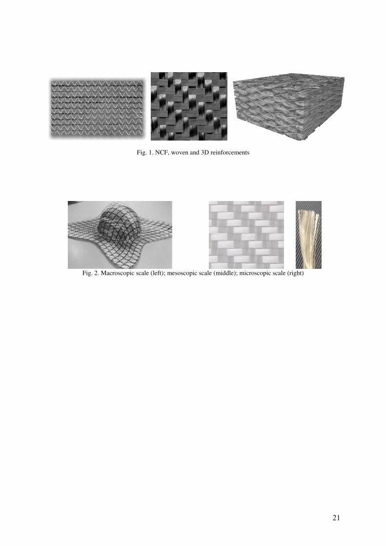
not undulated (Fig. 1a)(Yu et al, 2005; Lomov, 2011; Bel et al, 2012). Weaving is the

classical way to assemble fibres that are gathered in warp and weft yarns and interlaced by

weaving (Fig1b). 2D woven fabric are made up of a single layer of warp and weft yarns. In

3D fabric, the weaving concerns an important thickness and several layer of warp and weft

yarns (Fig. 1c)(Mouritz et al, 1999; Dufour et al, 2014). In order to obtain a composite part

with a given thickness, the UD, NCF and 2D woven reinforcement are stacked to form a

laminate. These material can be subject to delamination. This is avoided by 3D weavings.

Section 3 presents, a mechanical model for 3D composite reinforcement during forming and

its application to the simulations of hemispherical drawing and large three point bending.

2.2. Different scales for composite reinforcement analysis

Composite reinforcements are made up of fibres usually gathered in yarns (3000 to 48000

fibres per carbon yarn). These yarns are themselves assembled by weaving or stitching. Three

scales can be clearly distinguished for the analysis. These analyses can be made at the scale of

the part (macroscopic scale), at the scale of the yarn (mesoscopic scale), or at the fibre scale

4

(microscopic scale). These three scales are simultaneously present in a reinforcement. The

modelling and the simulations can be made at one of these three scale depending of the

objective. Simulation of reinforcements or prepreg forming is usually done at macroscopic

scale in order to determine the optimal conditions of a process, the directions of the fibres

after forming and possibly the onset of defects (in particular wrinkling)(Pickett et al, 1995;

Boisse et al, 1995; Hancock and Potter, 2005; Zouari et al, 2005; Jauffrès et al, 2010). The

objectives of mesoscopic analyses include performing virtual tests on one or some

representative elementary cells (Cai, 1992; Chen and Chou, 2000; Xue et al, 2005, Lomov et

al 2007, Charmetant et al, 2011; Nguyen et al, 2013). They also permit to determine the

properties of the deformed element cell, in particular the permeability of compacted or

sheared reinforcements (Lekakou et al, 1996; Loix et al, 2008). Section 4 presents the use of

X-ray computed tomography in order to build F.E. models for mesoscopic analyses that are as

close as possible to the real reinforcement.

Analyses are also performed at the scale of the fibre (microscopic scale) (Zhou et al, 2004;

Durville, 2010). At this scale the considered solids (here the fibres) are actually continuous.

For upper scales (mesoscopic and macroscopic) the mechanical model must take into account

the fibrous nature of the yarn or of the reinforcement that might be tricky. At the microscopic

scale, the fibre can be seen as a beam. But there are many fibers in a yarn (several thousands)

and much more in a preform. Microscopic scale analyses are presently limited to parts of

reinforcements with moderate size.

3. Continuous approach for 3D composite forming process analysis

A hyperelastic constitutive law for 3D layer to layer angle interlock preforms is proposed.

This model is macroscopic and aims to determine the strains and stresses of the whole 3D

preform. The strain energy potential is defined for elementary deformation modes

5

3.1. Hyperelastic constitutive equation

The potential energy is a function that can be written as a function of the right Cauchy-Green

strain tensor C :

w w C with .T

C F F (1)

The dependence of the strain energy potential on the material privileged directions can be

introduced explicitly. Structural tensors representative of the anisotropy of the material are

introduced. 3D interlock fabrics are made of warp and weft yarns which are perpendicular to

each other in the initial configuration. The 3D material has three privileged directions: the

warp direction 1M , the weft direction 2M and a third direction 3M , perpendicular to 1M

and 2M , (through the preform thickness). These directions define three structural tensors:

1 11M M M ; 2 22

M M M and 3 33M M M (2)

Taking (Boehler, 1978) into account, the strain energy density function of a hyperelastic law

is written as:

1 2 3 41 42 43 412 423 51 52 53, , , , , , , , , ,orth orthw w I I I I I I I I I I I (3)

where 1I , 2I , 3I are the invariants of C defined by:

2 2

1 2 3

1

2 I Tr C I Tr C Tr C I Det C (4)

and where:

4 : i ii iI C M M C M , 4 i jijI M C M

2 2

5 : i ii iI C M M C M (i = 1,3) (5)

are the mixed invariants corresponding to the structural tensors.

The contribution of each deformation mode is assumed to be independent from the others,

The strain energy density function is consequently the summation these contributions.

1

ni i

i i

w Iw

C I C

(6)

6

where Ii is the strain invariant of the ith deformation mode.

3.2. Physically based invariants.

A phenomenological approach is undertaken to build a physically motivated behavior law

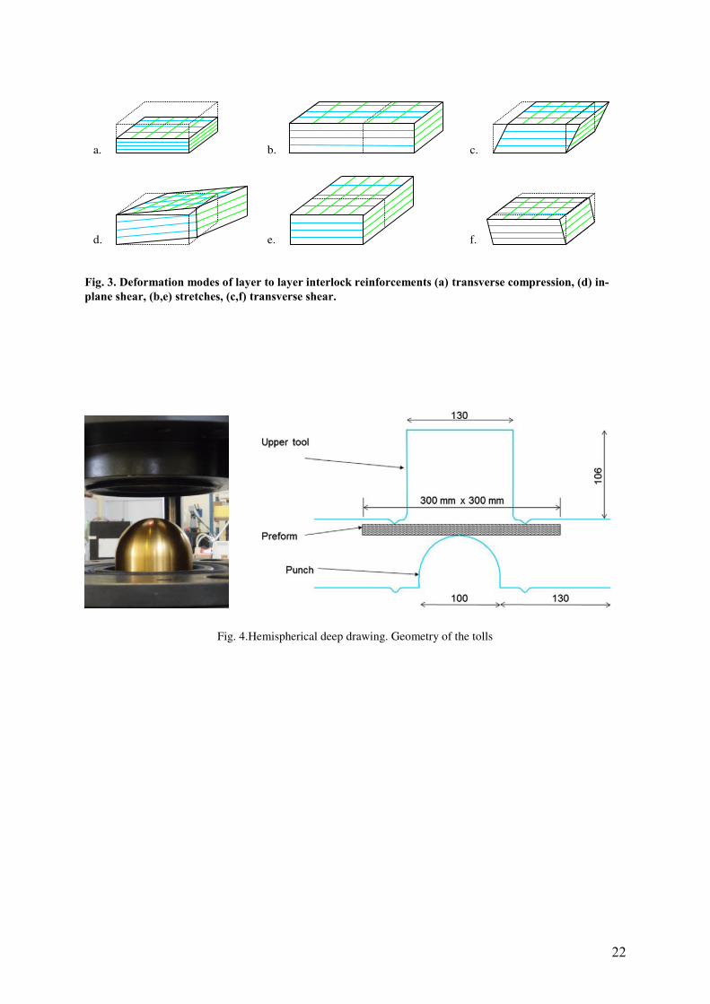
(Charmetant et al, 2012). Six deformation modes can be identified for a 3D composite

reinforcement: in-plane shear, transverse shear in warp and weft directions, stretch in the weft

and warp directions, and transverse compression. Each of this modes will be assigned a

physical invariant (Fig. 3).The aim of this procedure is to ease the identification process.

The stretch invariants in warp and weft directions are defined using the 𝐼41 and 𝐼42

4ln 1,2elongI I

(7)

The definition of the transverse compression invariant is more complex. This invariant is not

only linked to the third direction 3M . During a pure transverse shear solicitation for example,

the length of the material vector 3M will not change but the thickness of the preform will

decrease, The transverse compression invariant is consequently defined as the total volume

change divided by the two yarn stretches:

3

41 42

1ln

2comp

II

I I

(8)

The in-plane shear invariant can be linked to the angle variation 𝛾 between the material

directions 1M and 2M in the initial configuration, and 1m and 2m in the current

configuration. As 1M and 2M are perpendicular:

1 2

1 2

sinm m

m m

(9)

Consequently, the in-plane shear invariant is defined by:

421

41 42

sincp

II

I I (10)

7

As for the in-plane shear, the transverse shear invariants are defined by:

4 33

4 43

sin 1,2 ct

II

I I

(11)

The six deformation modes are assumed to be independent. The energy density is then

defined as the summation of the contributions of the six deformation modes:

6

1

( ) ( )

bw C w I (12)

The second Piola-Kirchhoff tensor is finally obtained by differentiation:

2

w I

SI C

(14)

3.3. Strain energy potential identification

Tension in warp and weft direction tests are performed to identify the tensile potential. The

transverse compaction strain energy density is identified from a compressive test. A bias

extension test is performed to identify the in-plane shear properties. In this case a Levenberg–

Marquardt algorithm is used to identify all the values. Finally a transverse shear test is used to

identify the part of the strain energy that is coming from this deformation. Details of the

identifications and the form given to the different potentials can be found in (Charmetant et

al, 2012).

3.4 Simulation of a hemispherical forming of a 3D interlock reinforcement.

The hemispherical deep drawing test is frequently used to analyse fabric reinforcements forming

experiments (Boisse et al, 1995; Yu et al, 2005; Jauffres et al, 2010). The hemisphere is doubly

curved and in-plane strains of the fabric are necessary to obtain the shape. In-plane shear strains

can cause wrinkles (Skordos et al, 2007 ; Boisse et al, 2011]. This wrinkles can be avoided thanks

to blank holders that add tensions to the reinforcement (Lee et al, 2007; Boisse et al, 2011]. The

8

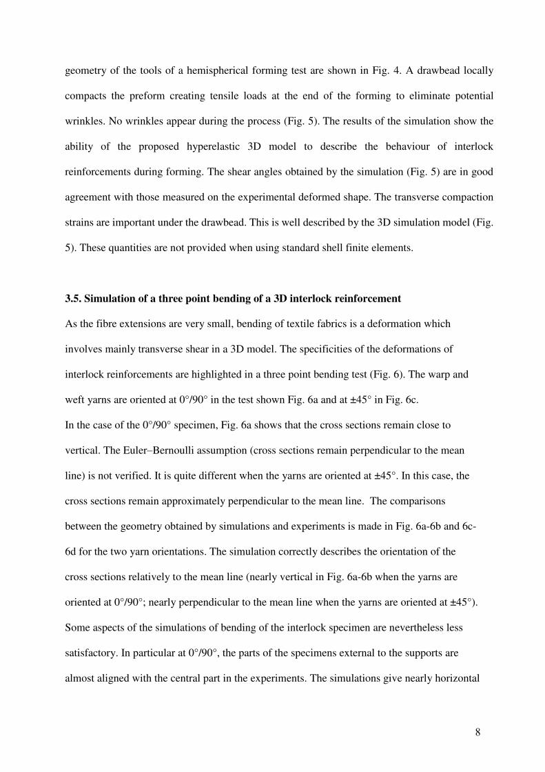
geometry of the tools of a hemispherical forming test are shown in Fig. 4. A drawbead locally

compacts the preform creating tensile loads at the end of the forming to eliminate potential

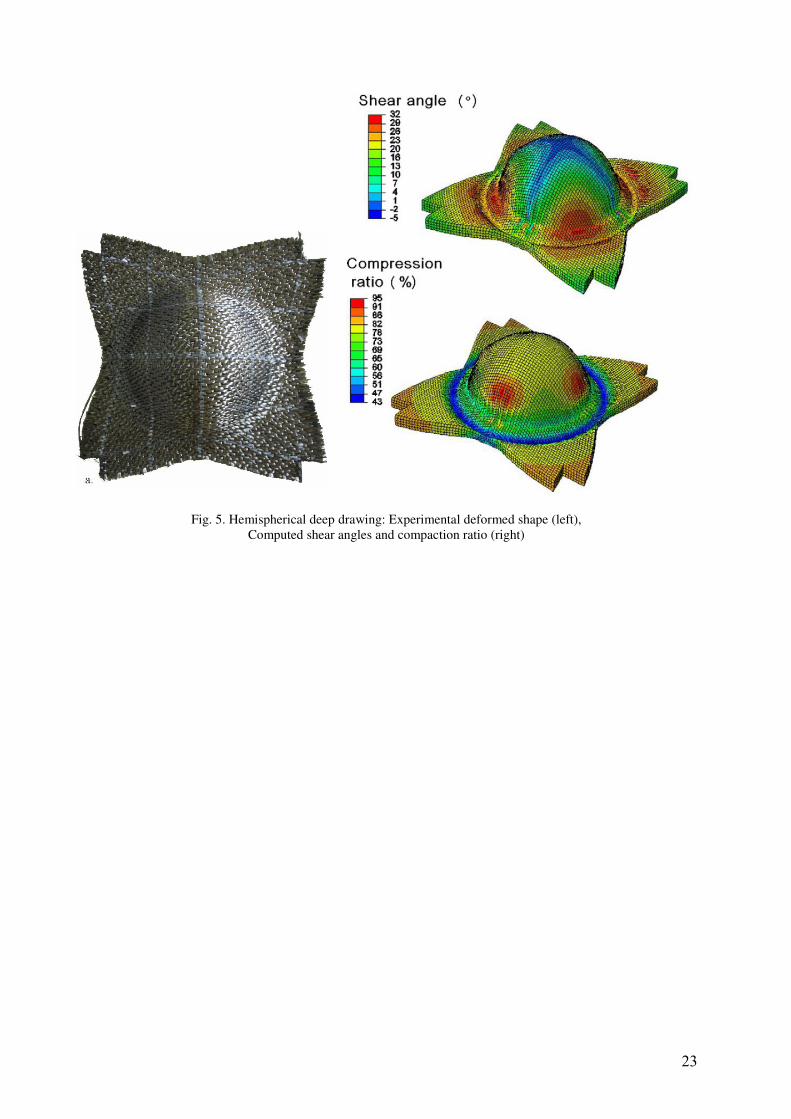
wrinkles. No wrinkles appear during the process (Fig. 5). The results of the simulation show the

ability of the proposed hyperelastic 3D model to describe the behaviour of interlock

reinforcements during forming. The shear angles obtained by the simulation (Fig. 5) are in good

agreement with those measured on the experimental deformed shape. The transverse compaction

strains are important under the drawbead. This is well described by the 3D simulation model (Fig.

5). These quantities are not provided when using standard shell finite elements.

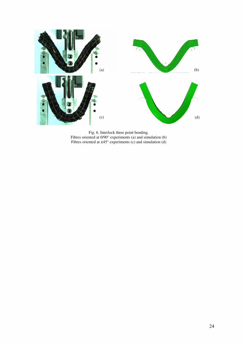
3.5. Simulation of a three point bending of a 3D interlock reinforcement

As the fibre extensions are very small, bending of textile fabrics is a deformation which

involves mainly transverse shear in a 3D model. The specificities of the deformations of

interlock reinforcements are highlighted in a three point bending test (Fig. 6). The warp and

weft yarns are oriented at 0°/90° in the test shown Fig. 6a and at ±45° in Fig. 6c.

In the case of the 0°/90° specimen, Fig. 6a shows that the cross sections remain close to

vertical. The Euler–Bernoulli assumption (cross sections remain perpendicular to the mean

line) is not verified. It is quite different when the yarns are oriented at ±45°. In this case, the

cross sections remain approximately perpendicular to the mean line. The comparisons

between the geometry obtained by simulations and experiments is made in Fig. 6a-6b and 6c-

6d for the two yarn orientations. The simulation correctly describes the orientation of the

cross sections relatively to the mean line (nearly vertical in Fig. 6a-6b when the yarns are

oriented at 0°/90°; nearly perpendicular to the mean line when the yarns are oriented at ±45°).

Some aspects of the simulations of bending of the interlock specimen are nevertheless less

satisfactory. In particular at 0°/90°, the parts of the specimens external to the supports are

almost aligned with the central part in the experiments. The simulations give nearly horizontal

9

external parts for this 0°/90° specimen. In addition the computed radius at the centre of the

two specimens are smaller than in experiments.

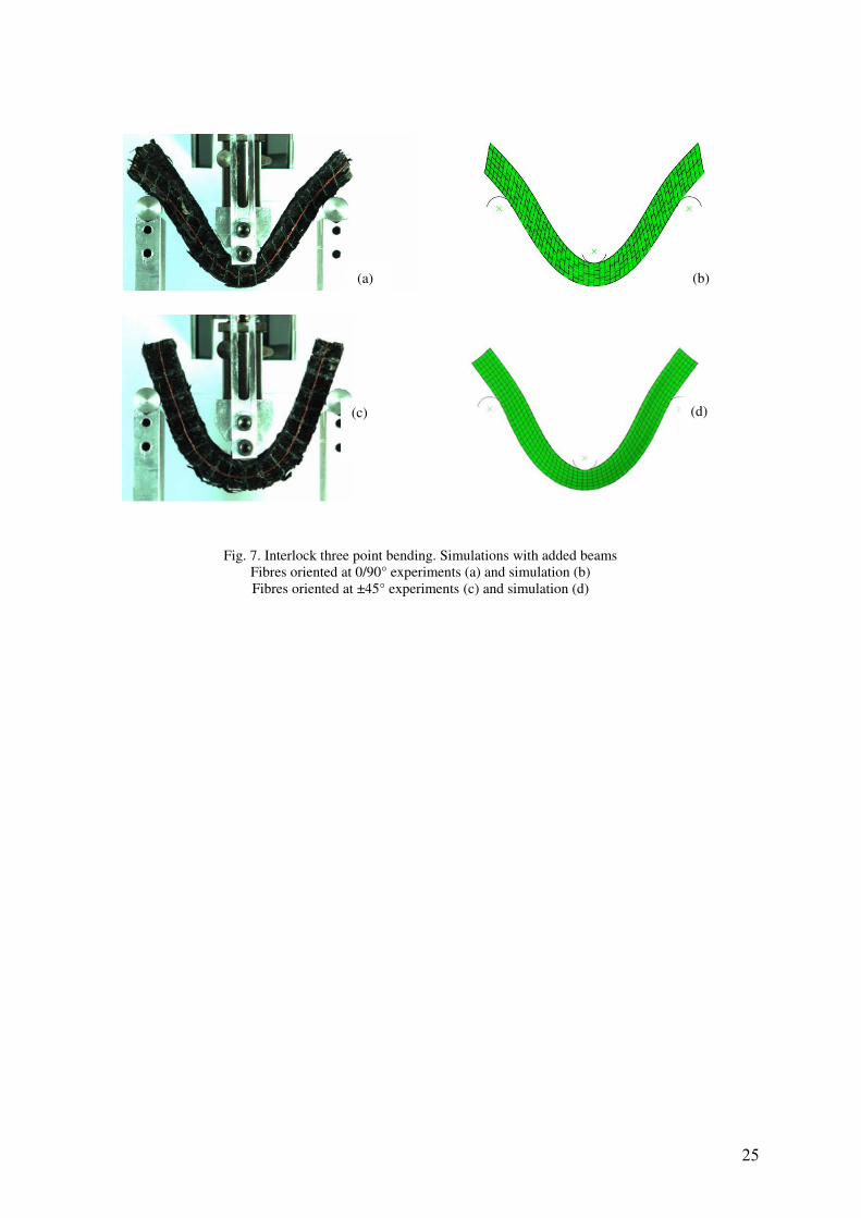
3.6. Simulation of a three point bending of a 3D interlock reinforcement adding a local

bending stiffness.

The differences between simulations based on the presented hyperelastic law and the

experiments in three point bending are related to local fibre bending rigidity. The local

bending stiffness of each fibre aims at keeping the external parts of the specimen aligned with

the central part. In addition these local bending rigidities increase the central radius of the

specimens. In the hyperelastic model presented above, as usual in classical continuum

mechanics there is no local miscrostructure that permits to introduce volume couples.

Generalized continuum mechanics approaches permit to model these couples (Forest, 1998

Maugin and Metrikine, 2010). In order to account for the fibre rigidities finite element beams

are added to the 3D continuous hyperelastic material in the warp and weft directions. These

beam elements bring the fibre bending stiffness. Fig. 7 shows the improvements obtain with

this approach. The external parts of the specimen are almost aligned with the central part both

in experiments and simulations. In addition the central radius of the specimen are in

agreement with experiments. This shows that the microstructure and in particular the bending

rigidity of the fibres should be taken into account in the mechanical behaviour of interlocks.

Studies have been conducted or are in progress to propose models based on generalized

continua (Ferretti et al, 2014, 2015; d’Agostino et al, 2015). However, the generalized

continuum models are complex and difficult to identify and implement. For interlock forming

simulation, the hyperelastic model described above and detailed in (Charmetant et al, 2012)

may be an interesting compromise between accuracy and simplicity.

10

4. Simulation at the mesoscopic scale based on X-ray computed tomography analysis

The mesoscopic analyses, i.e. analyses at the scale of the yarn, can be used as virtual test to

determine the mechanical properties of the reinforcement during forming. The influence of

different parameters and in particular of the geometry of the yarns and of the weaving can be

investigated without performing the experiments and consequently without manufacturing the

considered reinforcement. In mesoscopic analysis, the geometry of the yarns, their contacts are

described. But the fibres themselves are not modelled. The yarn is considered as a continuum.

The behaviour of the yarn is specific since it is made of thousands of fibres which can slide

with respect to each other. Different constitutive models have been proposed to describe the

specificity of this yarn mechanical behavior. The mechanical behavior can be modelled by a

hyperelastic law (Charmetant et al, 2011) or by a hypoelastic approach (Boisse et al, 2005;

Badel et al, 2008). X-ray tomography offers a powerful tool allowing the exploration of the

internal structure of the woven textile before and during its deformation. The technique used to

obtain a F.E. model at mesoscopic scale is described in the present section (Naouar et al, 2014).

A comparison is presented between experiments, simulations obtained from µCT and

simulation based on an idealized geometry in the case of a transverse compression test of a

carbon twill reinforcement.

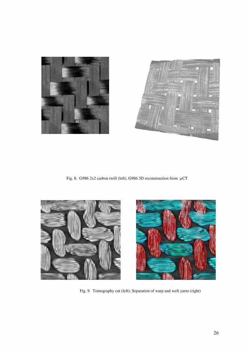
4.1. Determination of the reinforcement geometry by X-ray computed tomography.

A laboratory tomograph is used to acquire 3D images of the reinforcement (Herman, 1980;

Baruchel et al, 2000). As an example the analysis is performed on the Hexcel G0986® fabric

(Fig. 8a). It is a 2x2 carbon twill. Its 3D reconstruction obtained by X-ray computed

tomography is shown in Fig. 8. In order to define a finite element model of the representative

unit cell (RUC) of the fabric an image segmentation is performed to separate warp and weft

11

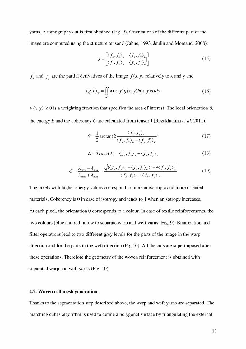
yarns. A tomography cut is first obtained (Fig. 9). Orientations of the different part of the

image are computed using the structure tensor J (Jahne, 1993, Jeulin and Moreaud, 2008):

, ,

, ,

x x w x y w

x y w y y w

f f f fJ

f f f f

(15)

xf and

yf are the partial derivatives of the image ( , )f x y relatively to x and y and

²

, ( , ) ( , ) ( , )w

R

g h w x y g x y h x y dxdy (16)

( , )w x y ≥ 0 is a weighting function that specifies the area of interest. The local orientation ,

the energy E and the coherency C are calculated from tensor J (Rezakhaniha et al, 2011).

,1

arctan(2 )2 , ,

x y w

y y w x x w

f f

f f f f

(17)

( ) , ,x x w y y w

E Trace J f f f f (18)

max min

max min

( , , )² 4 ,

, ,

y y w x x w x y w

x x w y y w

f f f f f fC

f f f f

(19)

The pixels with higher energy values correspond to more anisotropic and more oriented

materials. Coherency is 0 in case of isotropy and tends to 1 when anisotropy increases.

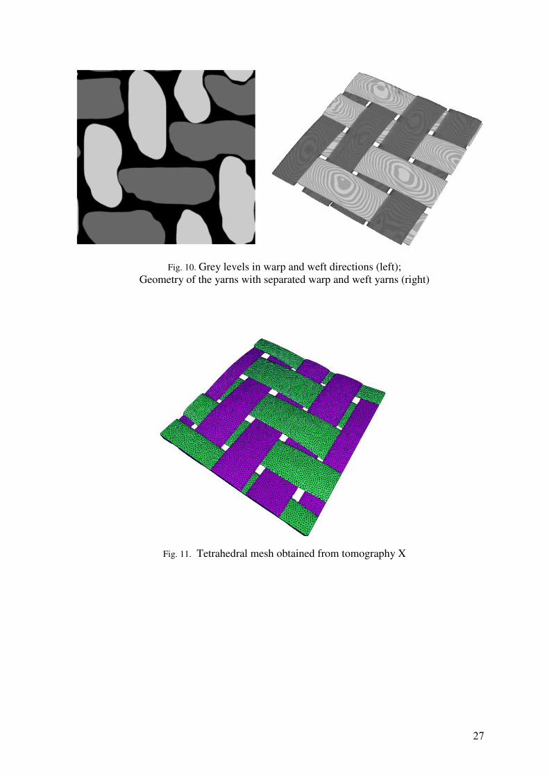
At each pixel, the orientation corresponds to a colour. In case of textile reinforcements, the

two colours (blue and red) allow to separate warp and weft yarns (Fig. 9). Binarization and

filter operations lead to two different grey levels for the parts of the image in the warp

direction and for the parts in the weft direction (Fig 10). All the cuts are superimposed after

these operations. Therefore the geometry of the woven reinforcement is obtained with

separated warp and weft yarns (Fig. 10).

4.2. Woven cell mesh generation

Thanks to the segmentation step described above, the warp and weft yarns are separated. The

marching cubes algorithm is used to define a polygonal surface by triangulating the external

12

surface of each yarn (Lorensen and Cline, 1987). A front algorithm (Jin and Tanner, 1993) is

used to obtain a volume mesh of each yarn. The initial front is made up of the external

triangles. Tetrahedral elements are generated step by step on the whole volume of the yarns

(Fig. 11).

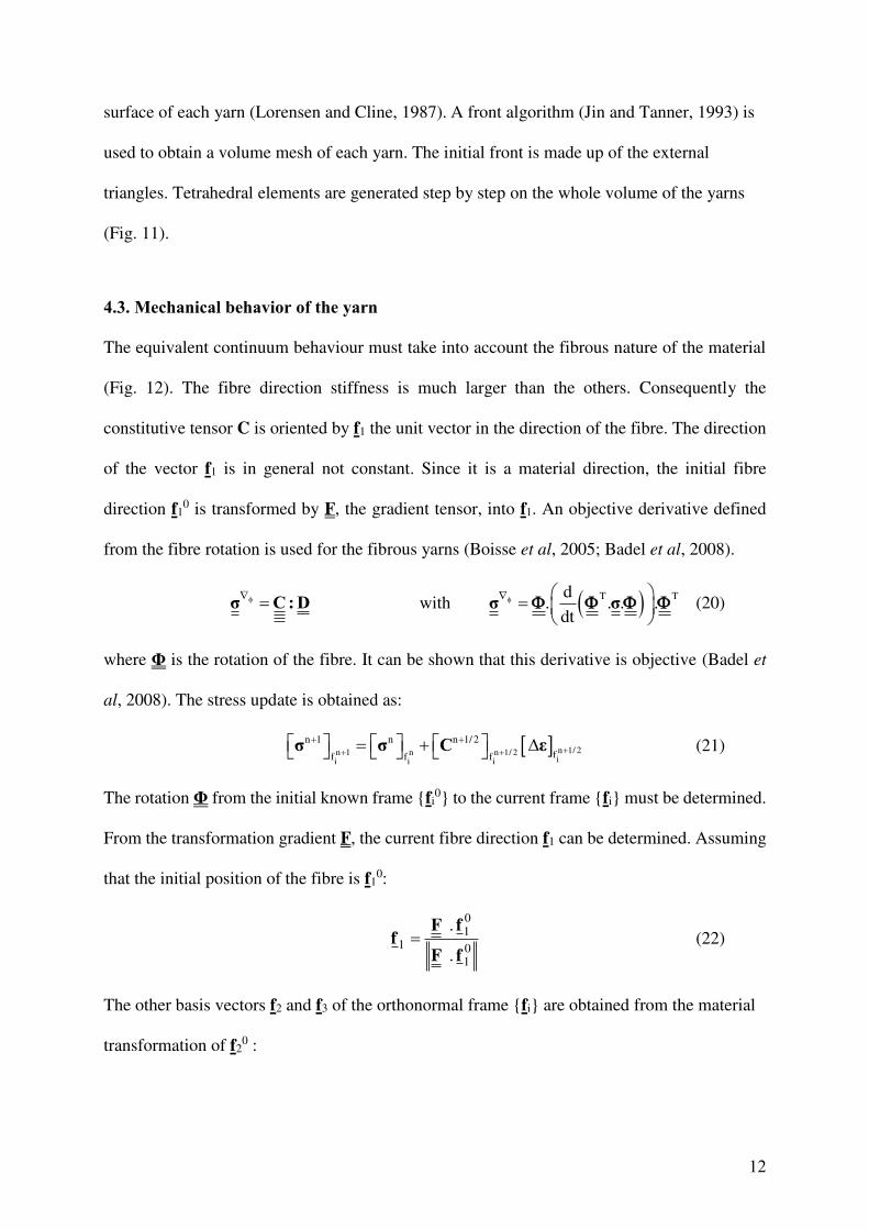
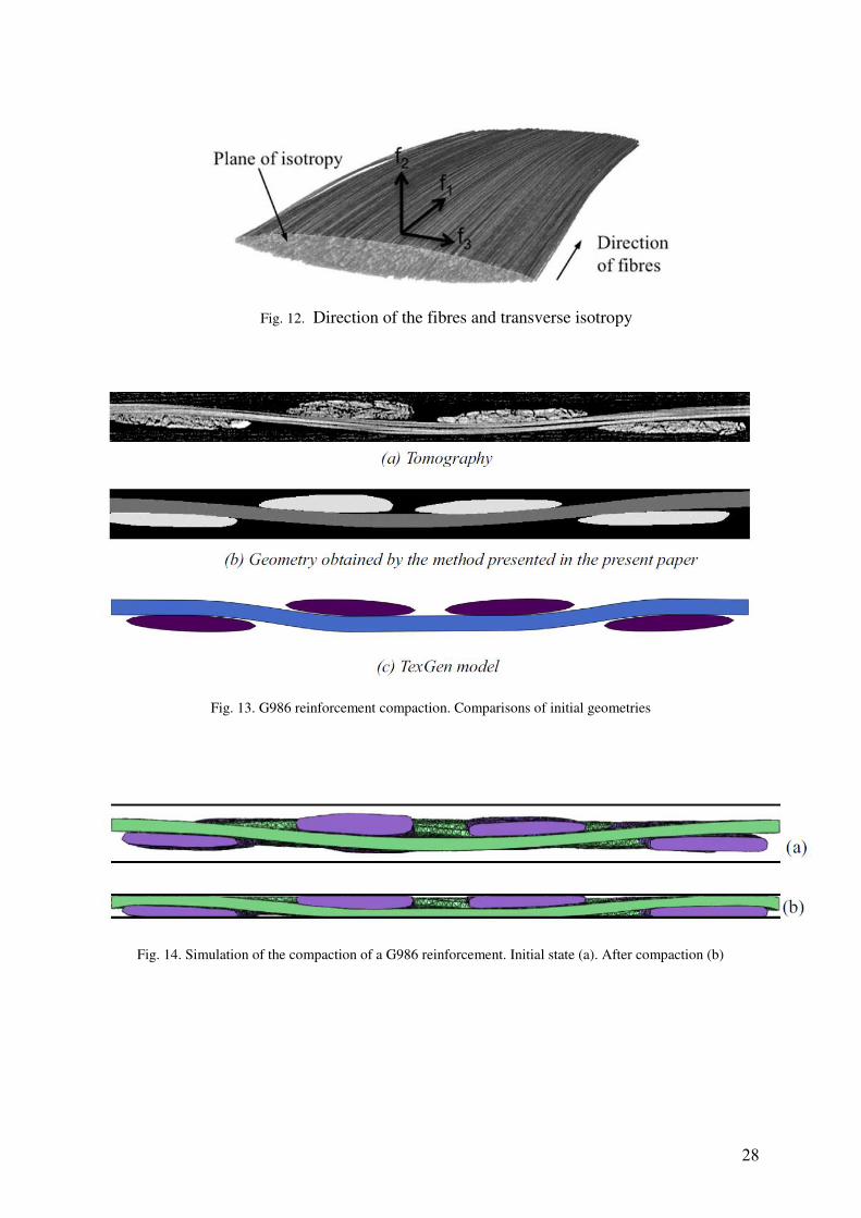
4.3. Mechanical behavior of the yarn

The equivalent continuum behaviour must take into account the fibrous nature of the material

(Fig. 12). The fibre direction stiffness is much larger than the others. Consequently the

constitutive tensor C is oriented by f1 the unit vector in the direction of the fibre. The direction

of the vector f1 is in general not constant. Since it is a material direction, the initial fibre

direction f10 is transformed by F, the gradient tensor, into f1. An objective derivative defined

from the fibre rotation is used for the fibrous yarns (Boisse et al, 2005; Badel et al, 2008).

σ C:D with T Td. . . .

dt

σ σ (20)

where Φ is the rotation of the fibre. It can be shown that this derivative is objective (Badel et

al, 2008). The stress update is obtained as:

n 1/ 2n 1 n n 1/ 2ii i i

n 1 n n 1/ 2

ff f f

σ σ C ε (21)

The rotation Φ from the initial known frame {fi0} to the current frame {fi} must be determined.

From the transformation gradient F, the current fibre direction f1 can be determined. Assuming

that the initial position of the fibre is f10:

01

1 01

.

.

F ff

F f (22)

The other basis vectors f2 and f3 of the orthonormal frame {fi} are obtained from the material

transformation of f20 :

13

0 0

2 2 1

2 3 1 20 0

2 2 1

. . . and

. . .

F f F f ff f f f

F f F f f (23)

Then the rotation Φ is obtained by:

00 0 0 0 0 0

i i j i j j i i ji

. Φ f f f f f f f f f (24)

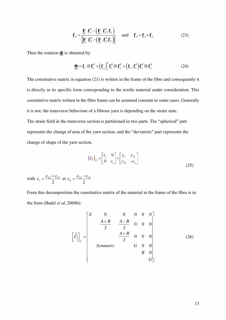
The constitutive matrix in equation (21) is written in the frame of the fibre and consequently it

is directly in its specific form corresponding to the textile material under consideration. This

constitutive matrix written in the fibre frame can be assumed constant in some cases. Generally

it is not; the transverse behaviour of a fibrous yarn is depending on the strain state.

The strain field in the transverse section is partitioned in two parts. The “spherical” part

represents the change of area of the yarn section, and the “deviatoric” part represents the

change of shape of the yarn section.

(25)

with 22 33

2s

et 22 33

2d

From this decomposition the constitutive matrix of the material in the frame of the fibre is in

the form (Badel et al, 2008b):

0 0 0 0 0

0 0 02 2

0 0 02

0 0

0

if

E

A B A B

A BC

Symmetry G

B

G

(26)

14

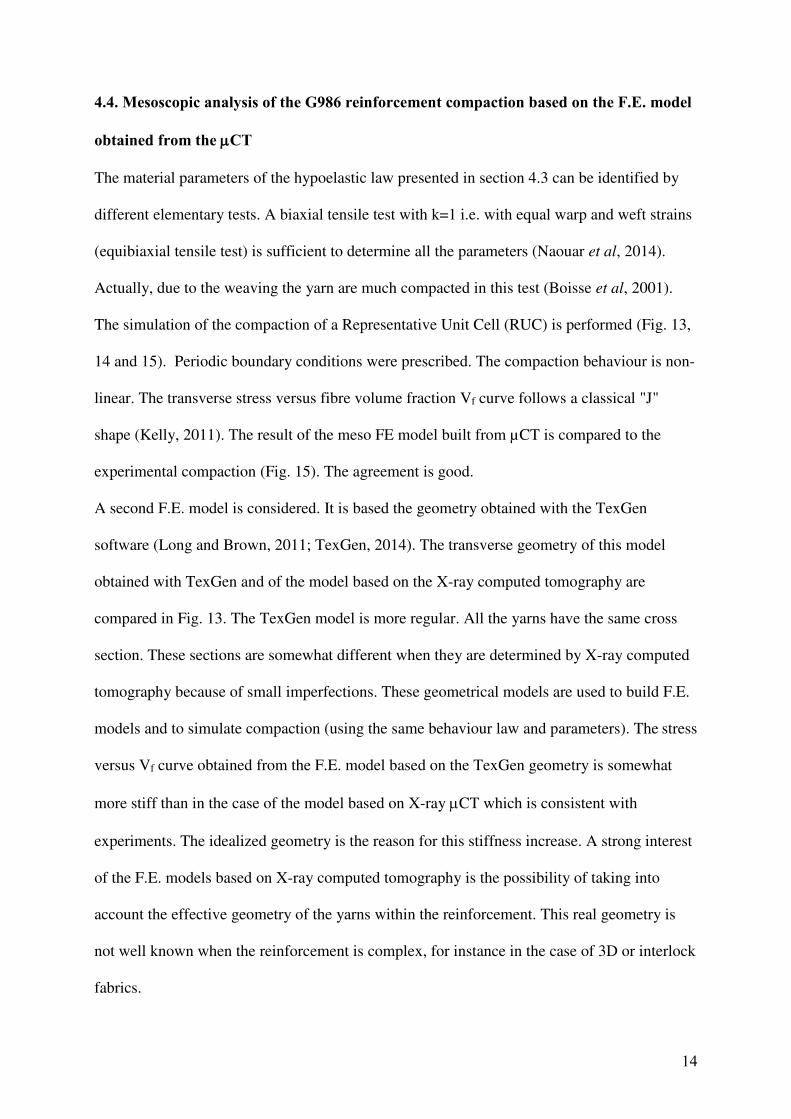
4.4. Mesoscopic analysis of the G986 reinforcement compaction based on the F.E. model

obtained from the CT

The material parameters of the hypoelastic law presented in section 4.3 can be identified by

different elementary tests. A biaxial tensile test with k=1 i.e. with equal warp and weft strains

(equibiaxial tensile test) is sufficient to determine all the parameters (Naouar et al, 2014).

Actually, due to the weaving the yarn are much compacted in this test (Boisse et al, 2001).

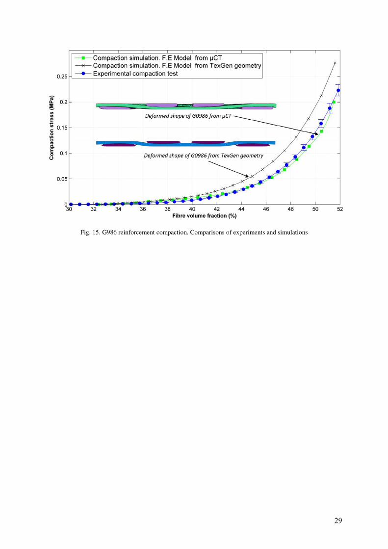
The simulation of the compaction of a Representative Unit Cell (RUC) is performed (Fig. 13,

14 and 15). Periodic boundary conditions were prescribed. The compaction behaviour is non-

linear. The transverse stress versus fibre volume fraction Vf curve follows a classical "J"

shape (Kelly, 2011). The result of the meso FE model built from µCT is compared to the

experimental compaction (Fig. 15). The agreement is good.

A second F.E. model is considered. It is based the geometry obtained with the TexGen

software (Long and Brown, 2011; TexGen, 2014). The transverse geometry of this model

obtained with TexGen and of the model based on the X-ray computed tomography are

compared in Fig. 13. The TexGen model is more regular. All the yarns have the same cross

section. These sections are somewhat different when they are determined by X-ray computed

tomography because of small imperfections. These geometrical models are used to build F.E.

models and to simulate compaction (using the same behaviour law and parameters). The stress

versus Vf curve obtained from the F.E. model based on the TexGen geometry is somewhat

more stiff than in the case of the model based on X-ray CT which is consistent with

experiments. The idealized geometry is the reason for this stiffness increase. A strong interest

of the F.E. models based on X-ray computed tomography is the possibility of taking into

account the effective geometry of the yarns within the reinforcement. This real geometry is

not well known when the reinforcement is complex, for instance in the case of 3D or interlock

fabrics.

15

5. Conclusions

The fibrous nature of composite reinforcements gives them a specific mechanical behavior.

The F.E. simulations of their deformation can avoid the development of forming processes by

try and error. The simulations can be made at macroscopic, mesoscopic and possibly

microscopic scale. Simulations of composite reinforcement forming processes are usually

performed at macroscopic scale. Shell finite elements are generally used to model each ply of

the laminate. For 3D reinforcements, 3D finite elements are necessary. A hyperelastic model

for these 3D analyses has been presented. It is based on the physical deformation modes of

the 3D reinforcements. It has shown to be able to describe the specific mechanical behavior of

3D interlock reinforcements in three point bending. The cross section of the specimen remains

nearly vertical for a 0/90° orientation of the yarns but are perpendicular to the mean line in the

case of a ±45° orientation. This is well depicted by the hyperelastic model. Nevertheless some

aspects of the deformation would require a generalized mechanics approach to take into

account the local bending stiffness of the fibres.

At the mesoscopic scale, the F.E. simulation gives the deformation of the internal textile

reinforcement structure. The analysis is usually made on a representative woven cell or on a

few of them. Probably in the future it can concern a whole preform. The result of the

simulation mainly depends on the quality of the initial F.E. model. X-Ray tomography is a

possible way to define meshes close to the real reinforcement. This approach will be

particularly interesting in the case of 3D fabrics for which geometry is complex and not

always well known.

16

References

Advani SG (1994). Flow and rheology in polymeric composites manufacturing. Elsevier

Amsterdam.

Badel P, Vidal-Sallé E, Boisse P (2008). Large deformation analysis of fibrous materials

using rate constitutive equations, Computers and Structures, 86 (11–12): 1164‑1175.

Badel P, Vidal-Salle E, Maire E, Boisse P (2008b). Simulation and tomography analysis of

textile composite reinforcement deformation at the mesoscopic scale. Compos Sci

Technol, 68(12): 2433–40.

Baruchel J, Buffiere JY, Maire E, Merle P, Peix G (2000). X-Ray Tomography in Material

Science. Baruchel J, Buffiere J., Maire E, Merle P, Peix G, editors. Hermes Science,

Bel S, Hamila N, Boisse P, Dumont F (2012). Finite element model for NCF composite

reinforcement preforming: Importance of inter-ply sliding. Composites Part A, 43 (12):

2269–2277.

Boisse P, Cherouat A, Gelin JC, Sabhi H (1995). Experimental Study and Finite Element

Simulation of Glass Fiber Fabric Shaping Process. Polymer Composites, 16(1): 83-95.

Boisse P, Gasser A, Hivet G (2001). Analyses of fabric tensile behaviour: determination of

the biaxial tension–strain surfaces and their use in forming simulations. Composites

Part A. 32 (10), 1395-1414

Boisse P, Gasser A, Hagège B, Billoet JL (2005). Analysis of the mechanical behavior of

woven fibrous material using virtual tests at the unit cell level. J. Mater. Sci., 40 (22):

5955‑5962.

Boisse P, Hamila N, Vidal-Sallé E, Dumont F (2011). Simulation of wrinkling during textile

composite reinforcement forming. Influence of tensile in-plane shear and bending stiffnesses.

Composites Science and Technology, 71 (5): 683–92.

Boehler JP (1978). Lois de comportement anisotropes des milieux continus. J Méc, 17:153–

70.

Cai Z, Gutowski T (1992). The 3-D deformation behavior of a lubricated fiber bundle. J

Comp Mater, 26:1207-37.

Charmetant A, Vidal-Salle E, Boisse P (2011). Hyperelastic modelling for mesoscopic

analyses of composite reinforcements. Composites Science and Technology, 71(14):

1623–1631

17

Charmetant A, Orliac JG, Vidal-Sallé E, Boisse P (2012). Hyperelastic model for large

deformation analyses of 3D interlock composite preforms, Composites Science and

Technology, 72 (12): 1352‑1360

Chen B, Chou TW (2000). Compaction of woven-fabric preforms: nesting and multi-layer

deformation. Composites Science and Technology, 60: 2223-2231

Dufour C, Wang P, Boussu F, Soulat D (2014). Experimental Investigation about Stamping

Behaviour of 3D Warp Interlock Composite Preforms. Appl Compos Mater 21:725–

738.

Durville D (2010). Simulation of the mechanical behaviour of woven fabrics at the scale of

fibers, Int J Mater Form, 3 (2): 1241–1251

Eberhardt C, Clarke A, Vincent M, Giroud T, Flouret S (2001). Fibre-orientation

measurements in short-glass-fibre composites II: a quantitative error estimate of the 2D

image analysis technique. Composites Science and Technology, 61 (13): 1961–1974.

Ferretti M, Madeo A, dell’Isola F, Boisse P (2014), Modeling the onset of shear boundary

layers in fibrous composite reinforcements by second-gradient theory, Zeitschrift für

angewandte Mathematik und Physik, 65, (3): 587-612

Forest S (1998). Cosserat overall modeling of heterogeneous materials. Mechanics Research

Communications, 25: 449-454

Fu SY, Lauke B, Mäder E, Yue CY, Hu X (2000). Tensile properties of short glass fiber and

short carbon fiber reinforced polypropylene composites; Composites part A, 31 (10):

1117–1125.

Hancock SG, Potter KD (2005). Inverse drape modelling - an investigation of the set of

shapes that can be formed from continuous aligned woven fibre reinforcements.

Composites: Part A, 36: 947-53.

Herman GT(1980). Image Reconstruction from Projections: The Fundamentals of

Computerized Tomography. Herman GT, editor. New York: Academic Press.

Jahne B (1993). Spatio-temporal image processing: Theory and scientific applications. Jahne

B, editor. Springer.

Jauffrès D, Sherwood JA, Morris CD, Chen J (2010). Discrete mesoscopic modeling for the

simulation of woven-fabric reinforcement forming, Int J Mater Form, 3: 1205-16.

Jeulin D, Moreaud M (2008). Segmentation of 2d and 3d textures from estimates of the local

orientation. Image Analysis & Stereology. 27: 183‑92. Jin H, Tanner R (1993).

18

Generation of unstructured tetrahedral meshes by advancing front technique.

International Journal for Numerical Methods in Engineering, 36(11):1805‑23.

Khan MA, Mabrouki T, Vidal-Sallé E, Boisse P (2010). Numerical and experimental analyses

of woven composite reinforcement forming using a hypoelastic behaviour. Application

to the double dome benchmark. J Mater Process Technol, 210:378–88.

Kelly P (2011). Transverse compression properties of composite reinforcements. Composite

reinforcements for optimum performance. Woodhead Publishing: 333‑366.

Laure P, Silva L, Vincent M (2011). Modelling short fibre polymer reinforcements for

composites in Composite reinforcements for optimum performance. Woodhead

Publishing Limited, 616-647.

Le Corre S, Orgéas L, Favier D, Tourabi A, Maazouz A, Venet V (2002). Shear and

compression behaviour of sheet moulding compounds. Composites Science and

Technology, 62 (4): 571–577.

Lee J, Hong S, Yu W, Kang T (2007). The effect of blank holder force on the stamp forming

behaviour of non-crimp fabric with a chain stitch. Compos Sci Technol, 67:357–66.

Lekakou C, Johari MAKB, Bader MG (1996). Compressibility and flow permeability of two-

dimensional woven reinforcements in the processing of composites, Polymer

Composites, 17 (5): 666-672.

Loix F, Badel P, Orgéas L, Geindreau C, Boisse P (2008). Woven fabric permeability: from

textile deformation to fluid flow mesoscale simulations. Composites Science and

Technology, 68: 1624–1630

Lomov SV, Ivanov DS, Verpoest I, Zako M, Kurashiki T, Nakai H, Hirosawa S (2007).

Meso-FE modelling of textile composites: Road map, data flow and algorithms.

Composites Science and Technology, 67: 1870–1891.Lomov SV (2011) Ed. Non-Crimp

Fabric Composites: Manufacturing, Properties and Applications, Woodhead Publishing

Limited.

Long AC, Brown LP (2011), Modelling the geometry of textile reinforcements for

composites: TexGen. Composite reinforcements for optimum performance. Woodhead

Publishing: 239-264.

Lorensen WE, Cline HE (1987). Marching cubes: A high resolution 3D surface construction

algorithm. Proceedings of the 14th annual conference on Computer graphics and

interactive techniques. ACM, New York, NY, USA:163‑9

19

Madeo A, d'Agostino MV, Giorgio I, Greco L, Boisse P (2015). Continuum and discrete

models for structures including (quasi-)inextensible elasticae with a view to the design

and modeling of composite reinforcement. Int J Sol Struct, in press.

Madeo A, Ferretti M, dell’Isola F, Boisse P (2015). Thick fibrous composite reinforcements

behave as special second gradient materials: three point bending of 3D interlocks,

Zeitschrift für angewandte Mathematik und Physik, in press.

Mark C, Taylor HM (1956). The fitting of woven cloth to surfaces, Journal of Textile

Institute, 47: 477-488.

Maugin GA, Metrikine V (eds) (2010). Mechanics of Generalized Continua: One hundred

years after the Cosserats, Advances in Mechanics and Mathematics 21, Springer.

Mouritz AP, Bannister MK, Falzon PJ, Leong KH (1999), Review of applications for

advanced three-dimensional fibre textile composites, Composites Part A, 30: 1445–

1461.

Naouar N, Vidal-Sallé E, Schneider J, Maire E, Boisse P (2014). Meso-scale FE analyses of

textile composite reinforcement deformation based on X-ray computed tomography,

Composite Structures, Volume 116: 165–176.

Nguyen QT, Vidal-Sallé E, Boisse P, Park CH, Saouab A, Breard J, Hivet G (2013).

Mesoscopic scale analyses of textile composite reinforcement compaction, Composites

Part B 44 (1): 231–241

Peng XQ, Cao J (2005). A continuum mechanics-based non-orthogonal constitutive model for

woven composite fabrics. Composites part A, 36 (6): 859–874.

Pickett AK, Queckbörner T, De Luca P, Haug E (1995). An explicit finite element solution

for the forming prediction of continuous fibre-reinforced thermoplastic sheets. Compos

Manuf, 6 (3–4): 237–43

Rezakhaniha R, Agianniotis A, Schrauwen JTC, Griffa A, Sage D, Bouten CVC, van de

Vosse FN, Unser M, Stergiopulos N (2011). Experimental investigation of collagen

waviness and orientation in the arterial adventitia using confocal laser scanning

microscopy. Biomechanics and Modeling in Mechanobiology, 11(3- 4): 461–473,

Rogers TG (1989). Rheological characterization of anisotropic materials, Composites, 20 (1):

21–27

Ruiz E, F. Trochu (2011). Flow modeling in composite reinforcements in Composite

reinforcements for optimum performance, Woodhead Publishing Limited, 588-615.

20

Skordos AA, Monroy Aceves C, Sutcliffe MPF (2007). A simplified rate dependent model of

forming and wrinkling of pre-impregnated woven composites. Composites Part A,

38:1318–30.

Spencer AJM (2000). Theory of fabric-reinforced viscous fluids. Composites Part A, 31: 1311–

1321

Ten Thije RHW, Akkerman R, Huétink J (2007). Large deformation simulation of anisotropic

material using an updated Lagrangian finite element method. Comput Methods Appl

Mech Eng, (196): 3141–50.

TexGen (2014). Available from: http://texgen.sourceforge.net/index.php/Main_Page

(accessed 15 December 2014)

Van Der Ween F (1991). Algorithms for draping fabrics on doubly curved surfaces.

International Journal of Numerical Method in Engineering, 31: 1414-1426.

Xue P, Cao J, Chen J (2005). Integrated micro/macro-mechanical model of woven fabric

composites under large deformation. Composite Structures, 70: 69–80

Yu WR, Pourboghrat F, Chung K, Zamploni M, Kang TJ (2002). Non-orthogonal

Constitutive Equation for Woven Fabric Reinforced Thermoplastic Composites.

Composites Part A. 33: 1095-1105.

Yu WR, Harrison P, Long A (2005). Finite element forming simulation for non-crimp fabrics

using a non-orthogonal constitutive equation. Composites: Part A, 36:1079–93.

Zhou G, Sun X, Wang Y (2004). Multi-chain digital element analysis in textile mechanics.

Compos Sci Technol, 64:239–44.

Zouari B, Daniel JL, Boisse P (2006). A woven reinforcement forming simulation method.

Influence of the shear stiffness. Computers and Structures, 84 (5-6): 351-363.

21

Fig. 1. NCF, woven and 3D reinforcements

Fig. 2. Macroscopic scale (left); mesoscopic scale (middle); microscopic scale (right)

22

Fig. 3. Deformation modes of layer to layer interlock reinforcements (a) transverse compression, (d) in-

plane shear, (b,e) stretches, (c,f) transverse shear.

Fig. 4.Hemispherical deep drawing. Geometry of the tolls

a. b. c.

f. e. d.

23

Fig. 5. Hemispherical deep drawing: Experimental deformed shape (left),

Computed shear angles and compaction ratio (right)

24

Fig. 6. Interlock three point bending.

Fibres oriented at 0/90° experiments (a) and simulation (b)

Fibres oriented at ±45° experiments (c) and simulation (d)

(a) (b)

(c) (d)

25

Fig. 7. Interlock three point bending. Simulations with added beams

Fibres oriented at 0/90° experiments (a) and simulation (b)

Fibres oriented at ±45° experiments (c) and simulation (d)

(a) (b)

(c) (d)

26

Fig. 8. G986 2x2 carbon twill (left), G986 3D reconstruction from CT

Fig. 9. Tomography cut (left); Separation of warp and weft yarns (right)

a) b)

27

Fig. 10. Grey levels in warp and weft directions (left);

Geometry of the yarns with separated warp and weft yarns (right)

Fig. 11. Tetrahedral mesh obtained from tomography X

28

Fig. 12. Direction of the fibres and transverse isotropy

Fig. 13. G986 reinforcement compaction. Comparisons of initial geometries

Fig. 14. Simulation of the compaction of a G986 reinforcement. Initial state (a). After compaction (b)

29

Fig. 15. G986 reinforcement compaction. Comparisons of experiments and simulations