Macroscopic Balance Equations

9

Macroscopic Balance Equations

Paul K. Andersen and Sarah W. Harcum

New Mexico State University, Las Cruces, New Mexico

The prevention of waste and pollution requires an understanding of numeroustechnical disciplines, including thermodynamics, heat and mass transfer, fluidmechanics, and chemical kinetics. This chapter summarizes the basic equationsand concepts underlying these seemingly disparate fields.

1 MACROSCOPIC BALANCE EQUATIONS

A balance equation accounts for changes in an extensive quantity (such as massor energy) that occur in a well-defined region of space, called the control volume(CV). The control volume is set off from its surroundings by boundaries, calledcontrol surfaces (CS). These surfaces may coincide with real surfaces, or theymay be mathematical abstractions, chosen for convenience of analysis. If mattercan cross the control surfaces, the system is said to be open; if not, it is said tobe closed.

1.1 The General Macroscopic Balance

Balance equations have the following general form:

Copyright 2002 by Marcel Dekker, Inc. All Rights Reserved.

dXdt

= ∑(XCS,i

⋅ )i + (X⋅ )gen (1)

where X is some extensive quantity. A dot placed over a variable denotes a rate;for example, (X⋅ )i is the flow rate of X across control surface i. The terms of Eq. (1)can be interpreted as follows:

dXdt

= rate of change of X inside the control volume

∑(XCS,i

⋅ )i = sum of flow rates of X across the control surfaces

(X⋅ )gen = rate of generation of X inside the control volume

Flows into the control volume are considered positive, while flows out of thecontrol volume are negative. Likewise, a positive generation rate indicates that Xis being a created within the control volume; a negative generation rate indicatesthat X is being consumed in the control volume.

The variable X in Eq. (1) represents any extensive property, such as thoselisted in Table 1. Extensive properties are additive: if the control volume is

TABLE 1 Extensive Quantities

Quantity Flow rate (CS i) Generation rate

Total mass, m m⋅i m⋅

gen = 0 (conservation ofmass)

Total moles, N N⋅i N

⋅gen

Species mass, mA (m⋅A)i (m⋅

A)genSpecies moles, NA (N⋅

A)i (N⋅A)gen

Energy, E E⋅i = Q

⋅i + W

⋅i + m⋅

i E^

iE⋅i = Q

⋅i + W

⋅i + N

⋅i E

~i

E⋅gen = 0 (conservation ofenergy)

Entropy, S S⋅i = Q

⋅i /Ti + m⋅

i S^

iS⋅i = Q

⋅i /Ti + N

⋅i S

~i

S⋅gen ≥ 0 (second law ofthermodynamics)

Momentum, p = mv p⋅ i = m⋅i vi p⋅ gen = F (Newton’s second

law of motion)

Notes:

Q⋅

i ≡ heat transfer rate through CS i

W⋅

i ≡ work rate (power) at CS i

E^

i ≡ energy per unit mass of stream i; E~

i ≡ energy per unit mole of stream i

S^

i ≡ entropy per unit mass of stream i; S~

i ≡ entropy per unit mole of stream i

Ti ≡ absolute temperature of CS i

F ≡ net force acting on control volume


subdivided into smaller volumes, the total quantity of X in the control volumeis just the sum of the quantities in each of the smaller volumes. Balance equationsare not appropriate for intensive properties such as temperature and pressure,which may be specified from point to point in the control volume but are notadditive.

It is important to note that Eq. (1) accounts for overall or gross changes inthe quantity of X that is contained in a system; it gives no information about thedistribution of X within the control volume. A differential balance equation maybe used to describe the distribution of X (see Section 2.2).

Equation (1) may be integrated from time t1 to time t2 to show the changein X during that time period:

∆X = ∑(X)iCS,i

+ (X)gen (2)

1.2 Total Mass Balance

Material is conveniently measured in terms of the mass m. According to Einstein’sspecial theory of relativity, mass varies with the energy of the system:

m⋅ gen = 1

c2dEdt

(special relativity) (3)

where c = 3.0 × 108 m/s is the speed of light in a vacuum. In most problems ofpractical interest, the variation of mass with changes in energy is not detectable,and mass is assumed to be conserved—that is, the mass-generation rate is takento be zero:

m⋅ gen = 0 (conservation of mass) (4)

Hence, the mass balance becomes

dmdt

= ∑(CS,i

m⋅ )i (5)

1.3 Total Material Balance

The quantity of material in the CV can be measured in moles N, a mole being6.02 × 1023 elementary particles (atoms or molecules). The rate of change ofmoles in the control volume is given by

dNdt

= ∑(NCS,i

⋅ )i + (N⋅ )gen (6)

where (N⋅)i is the molar flow rate through control surface i and (N⋅)gen is the molar


generation rate. In general, the molar generation rate is not zero; the determina-tion of its value is the object of the science of chemical kinetics (Section 4.2).

1.4 Macroscopic Species Mass Balance

A solution is a homogenous mixture of two or more chemical species. Solutionsusually cannot be separated into their components by mechanical means. Con-sider a solution consisting of chemical species A, B, . . . . For each of thecomponents of the solution, a mass balance may be written:

dmA

dt= ∑(

CS,i

m⋅ A )i + (m⋅ A )gen

dmB

dt= ∑(

CS,i

m⋅ B )i + (m⋅ B )gen (7)

...

Conservation of mass requires that the sum of the constituent mass generationrates be zero:

(m⋅ A )gen + (m⋅ B )gen + . . . = 0 (conservation of mass) (8)

1.5 Macroscopic Species Mole Balance

The macroscopic species mole balances for a solution are

dNA

dt= ∑(N

CS,i

⋅A )i + (N⋅ A )gen

dNB

dt= ∑(N

CS,i

⋅B )i + (N⋅ B )gen (9)

...

In general, moles are not conserved in chemical or nuclear reactions. Hence,

(N⋅ A )gen + (N⋅ B )gen + . . . = N⋅gen (10)

1.6 Macroscopic Energy Balance

Energy may be defined as the capacity of a system to do work or exchange heatwith its surroundings. In general, the total energy E can expressed as the sum ofthree contributions:


E = K + Φ + U (11)

where K is the kinetic energy, Φ is the potential energy, and U is the internal energy.Energy can be transported across the control surfaces by heat, by work, and

by the flow of material. Thus, the rate of energy transport across control surfacei is the sum of three terms:

E⋅

i = Q⋅

i + W⋅

i + m⋅ i E^

i (12)

where Q⋅i is the heat transfer rate, W

⋅i is the working rate (or power), m⋅ i is the

mass flow rate, and E^

i is the specific energy (energy per unit mass).Energy is conserved, meaning that the energy generation rate is zero:

E⋅

gen = 0 (conservation of energy) (13)

Therefore, the energy of the control volume varies according to

dEdt

= ∑(CS,i

Q⋅ + W

⋅ + m⋅ E^ )i (14)

The energy flow rate can also be written in terms of the molar flow rateN⋅i and the molar energy E

~i. Hence, the energy balance can be written in the

equivalent form

dEdt

= ∑(QCS,i

⋅ + W⋅ + N

⋅E~ )i (15)

1.7 Entropy Balance

Entropy is a measure of the unavailability of energy for performing useful work.Entropy may be transported across the system boundaries by heat and by the flow ofmaterial. Thus, the rate of entropy transport across control surface i is given by

S⋅i =

Q⋅i

Ti+ m⋅ i S

^

i (16)

where Q⋅

i is the heat transfer rate through control surface i, Ti is the absolutetemperature of the control surface, m⋅ i is the mass flow rate through the controlsurface, and S

^

i is the specific entropy or entropy per unit mass. In terms of themolar flow rate and the molar entropy S

~i, the entropy transport rate is

S⋅i =

Q⋅i

Ti+ N

⋅i S

~i (17)


According to the second law of thermodynamics, entropy may be created—but not destroyed—in the control volume. The entropy generation rate thereforemust be non-negative:

S⋅

gen ≥ 0 (second law of thermodynamics) (18)

Processes for which the entropy generation rate vanishes are said to be reversible.Most real processes are more or less irreversible.

In terms of mass flow rates, the entropy balance is

dSdt

= ∑CS,i

Q⋅

T+ m⋅ S

i

+ S⋅

gen (19)

If molar flow rates are used instead, the entropy balance is

dSdt

= ∑CS,i

Q⋅

T+ N

⋅S~i

+ S⋅gen (20)

1.8 Macroscopic Momentum Balance

The momentum p is defined as the product of mass and velocity. Because velocityis a vector—a quantity having both magnitude and direction—momentum is alsoa vector. Momentum can be transported across the system boundaries by the flowof mass into or out of the control volume:

p⋅ i = (m⋅ v )i (21)

According to Newton’s second law of motion, momentum is generated by the netforce F that acts on the control volume:

p⋅ gen = F (Newton’s second law) (22)

Hence, the momentum balance takes the form

dmvdt

= ∑CS,i

m⋅ vi + F (23)

Because this is a vector equation, it can be written as three component equations.In Cartesian coordinates, the momentum balance becomes

x momentum: dmvx

dt= ∑

CS,i

m⋅ vx

i + Fx


y momentum: dmvy

dt= ∑

CS,i

m⋅ vy

i + Fy (24)

z momentum: dmvz

dt= ∑

CS,i

m⋅ vz

i + Fz

2 DIFFERENTIAL BALANCE EQUATIONS

As noted previously, macroscopic balance equations account only for overall orgross changes that occur within a control volume. To obtain more detailedinformation, a macroscopic control volume can be subdivided into smaller controlvolumes. In the limit, this process of subdivision creates infinitesimal controlvolumes described by differential balance equations.

2.1 General Differential Balance Equation

The general macroscopic balance for the extensive property X is Eq. (1):

dXdt

= ∑CS,i

(X⋅ )i + (X⋅ )gen (1)

Division by the system’s volume V yields

ddt

XV

= ∑CS,i

X⋅i

V+

X⋅gen

V

The differential or microscopic balance equation results from taking the limit asV → 0:

∂[X]∂ = −∇ ⋅ (X) + [X⋅ ]gen (25)

where [X] is read as “the concentration of X” and X is “the flux of X.” The termsof this equation can be interpreted as follows:

∂∂t

[X] = rate of change of the concentration of X

−∇ ⋅ (X) = net influx of X

[X]gen = generation rate of X per unit volume

The flux X is the rate of transport per unit area, where the area is orientedperpendicular to the direction of transport. In Cartesian (x, y, z) coordinates, Xmay be defined as


X =X⋅x

Axi +

X⋅y

Ayj +

X⋅z

Azk

Here, Ax, Ay, and Az are the areas perpendicular to the x, y, and z directions,respectively; (i, j, k) are the (x, y, z) unit vectors. In Cartesian coordinates, thedel operator ∇ takes the form

∇ = ∂∂x

i + ∂∂y

j + ∂∂z

k

The form of the del operator in other coordinate systems may be found in textson fluid mechanics and transport phenomena (1–4).

Table 2 shows the concentrations, fluxes, and volumetric generation termsfor the extensive quantities considered in this chapter.

2.2 Differential Total Mass Balance

Assuming conservation of mass (ρgen = 0), the differential mass balance can bewritten as

TABLE 2 Concentrations, Fluxes, and Volumetric Generation

Quantity FluxVolumetric

generation rate

Total mass, [m] = ρ m = ρv ρ⋅ gen = 0 (conservation ofmass)

Total moles, [N] = c N = cv c⋅ genSpecies mass, [mA] = ρA mA = ρAv + jA (ρ⋅ A)genSpecies moles, [NA] = cA NA = cAv + JA (c⋅ A)genEnergy, [E] = e E = q + σ ⋅ v + mE

^

E = q + σ ⋅ v + NE~

e⋅ gen = 0 (conservationof energy)

Entropy, [S] = s S = q/T + mS^

S = q/T + NS~

s⋅ gen ≥ 0 (second law ofthermodynamics)

Momentum, [p] = ρv P = mv = ρvv f = −∇ ⋅ σ + b (second lawof motion)

Notes:

b ≡ body force per unit volume

jA ≡ diffusive mass flux of species A

JA ≡ diffusive molar flux of species A

f ≡ total force per unit volume

q ≡ heat flux

σ ≡ material stress

v ≡ fluid velocity


∂ρ∂t

= −∇ ⋅ (m) (26)

where m is the mass flux. It is more common to write the mass flux in terms ofthe density and velocity, m = ρv. Hence,

∂ρ∂t

= −∇ ⋅ (ρv) (27)

Equation (27) is called the continuity equation; it is one of the basic equations offluid mechanics.

2.3 Differential Total Material Balance

The differential material balance is

∂c∂t

= −∇ ⋅ (N) + c⋅ gen (28)

where N is the molar flux. In the absence of chemical or nuclear reactions,c⋅ gen = 0.

2.4 Differential Species Balances

Consider a solution consisting of component species A, B, . . . . In general, achemical species in such a solution may be transported by convection and bydiffusion. Convection is transport by the bulk motion of the solution. Theconvective flux of species A is the product of the mass concentration ρA and thesolution velocity v:

ρAv = convective (mass) flux of A

Diffusion is the transport of a species resulting from gradients of concentration,electrical potential, temperature, pressure, and so on. The diffusive flux of speciesA is denoted by jA:

jA = diffusive (mass) flux of A

The overall material flux is the sum of the convective and diffusive fluxes:

mA = ρAv + jA (29)

A differential mass balance may be written for each of the components of thesolution:

∂ρA

∂t= −∇ ⋅ (ρAv + jA) + (ρ⋅ A)gen


∂ρB

∂t= −∇ ⋅ (ρBv + jB) + (ρ⋅ B)gen (30)

...

Conservation of mass requires that the constituent mass generation rates sumto zero:

(ρ⋅ A)gen + (ρ⋅ B)gen + . . . = 0 (conservation of mass ) (31)

2.5 Differential Species Material Balance

The total molar flux of species A is the sum of the convective and diffusivemolar fluxes:

NA = cAv + JA (32)

where cAv is the convective molar flux and JA is the diffusive molar flux:

cAv = convective (molar) flux of A

JA = diffusive (molar) flux of A

The differential material balances for a solution consisting of species A, B, . . . are

∂cA

∂t= −∇ ⋅ (cAv + JA) + (c⋅ A)gen

∂cB

∂t= −∇ ⋅ (cBv + JB) + (c⋅ B)gen (33)

...

The sum of the constituent molar generation terms is the total molar volumetricgeneration rate:

(c⋅ A)gen + (c⋅ B)gen + . . . = c⋅ gen (34)

2.6 Differential Energy Balance

Energy may be transported by heat, by work, and by convection. Thus, the energyflux can be written as the sum of three terms:

(35)

where q is the heat flux, is the stress tensor (defined as the force per unit area),and mE

^ is the convective energy flux.

E = q + � ⋅ v + mE^

�


As used in Eq. (35), the stress tensor σ accounts for the forces exerted onthe surface of the differential control volume by the surrounding material.Multiplying the stress by the material velocity v gives the rate of work done(per unit area) on the surface of the control volume:

Rate of work by material stresses (per unit area) = σ ⋅ v

Conservation of energy requires that the energy generation rate be zero:

e⋅ gen = 0 (conservation of energy) (36)

The differential energy balance may be written as

∂e∂t

= −∇ ⋅ (q + σ ⋅ v + mE^ ) (37)

It is common practice to express the energy concentration as the product ofthe mass density and the specific energy: e = ρE

^. Hence, the energy balance

becomes

∂ρE^

∂t= −∇ ⋅ (q + σ ⋅ v + mE

^ ) (38)

If the material flux is measured in moles, the energy balance may be writtenin the equivalent form

∂ρE^

∂t= −∇ ⋅ (q + σ ⋅ v + NE

^ ) (39)

2.7 Differential Entropy Balance

Entropy may be transported by heat transfer and by convection. Thus, the entropyflux can be written as the sum of two terms:

S = qT

+ mS^

(40)

According to the second law of thermodynamics, the entropy generationrate must be non-negative:

s⋅ gen ≥ 0 (second law of thermodynamics) (41)

The differential entropy balance is

∂s∂t

= −∇ ⋅ qT

+ mS^

+ s⋅ gen (42)

�


If the molar flux is used instead of the mass flux, the entropy balancebecomes

∂s∂t

= −∇ ⋅ qT

+ NS~

+ s⋅ gen (43)

2.8 Differential Momentum Balance

The momentum concentration is the product of density and velocity: [p] = ρv.The momentum flux is the product of the momentum concentration and thevelocity: P = ρvv. The differential momentum balance is

∂ρv∂t

= −∇ ⋅ (ρvv) + f (44)

where f is the net force (per unit volume) acting on the control volume. In mostfluid systems, f is the sum of a stress term and a body-force term:

f = −∇ ⋅ σ + b (45)

The most important body force is gravity, for which b = ρg.The momentum balance becomes

∂ρv∂t

= −∇ ⋅ (ρvv) − ∇ ⋅ σ + b (46)

3 FLUX AND TRANSPORT EQUATIONS

In most cases, balance equations are not sufficient by themselves; additionalequations are needed to compute the fluxes and transport rates.

3.1 Diffusive Material Fluxes

As shown before, the overall material flux is the sum of the convective anddiffusive fluxes:

mA = ρAv + jA (47)

NA = cAv + JA (48)

The diffusive flux (jA or JA) is driven by gradients of concentration, electricalpotential, temperature, pressure, and so on. In the simplest situations, the rate ofdiffusion can be described by some variation of Fick’s law:

jA = ρDA∇ωA (49)

JA = −cDA∇χA (50)

where ωA is the mass fraction of A, χA is the mole fraction of A, and DA is the


diffusion coefficient or diffusivity of A. In some cases, other models may berequired for describing diffusion (see Refs. 4 and 5).

3.2 Heat Conduction

Heat conduction (also called heat diffusion) is the transport of thermal energy byrandom molecular motion. Conduction is driven by a temperature gradient. Inmost cases, the heat flux can be described by Fourier’s law:

q = −k∇T (51)

where k is the conductivity of the material. Conductivity values may be found inmany standard handbooks and heat transfer textbooks (9,10).

3.3 Radiation Heat Transfer

Radiation is the transport of energy by electromagnetic waves. Radiative heattransfer tends to be especially important at high temperatures, such as occur incombustion. Consider an object having a surface temperature Ts. The magnitudeof the radiation heat flux leaving the surface of the object is given by theStefan-Boltzmann law:

|qrad| = εσTs4 (52)

where σ is the Stefan-Boltzmann constant, a universal constant (σ = 5.67 × 10−8

W/m2 K4); and ε is the emissivity, a material property. Values of the emissivityfor many different materials are tabulated in standard handbooks (9,10).

3.4 Fluid Stress

The stress tensor appears in both the differential energy balance and thedifferential momentum balance. In general, stress is defined as force per unit area.The force and the area can be represented as vectors having magnitude anddirection:

F = (Fx,Fy,Fz) and A = (Ax, Ay, Az) (53)

Stress is a tensor having a magnitude and two directions. For example, the yxcomponent of the stress tensor is*

σyx =Fx

Ay(54)

The stress tensor is often represented as a 3 × 3 matrix having nine components:

�

�

*Some texts transpose the subscripts, so that σij = Fi /Aj.


=

σxx

σyx

σzx

σxy

σyy

σzy

σxz

σyz

σzz

=

Fx/Ax

Fx/Ay

Fx/Az

Fy/Ax

Fy/Ay

Fy/Az

Fz/Ax

Fz/Ay

Fz/Az

(55)

If the force is directed perpendicular to the area on which it acts, the resultis a normal stress. If the force acts tangentially to the area, the result is a shearstress. Thus, the diagonal elements of the stress tensor are normal stresses, andthe off-diagonal elements are shear stresses:

Normal stresses: σxx, σyy, σzz

Shear stresses: σxy, σxz, σyx, σyz, σzx, σzy

For a fluid, it is customary to resolve the stress tensor into two components:

(56)

where P is the fluid pressure, is the identity tensor, and is the viscous stresstensor. In matrix notation,

σxx

σyx

σzx

σxy

σyy

σzy

σxz

σyz

σzz

= −P

100

010

001

+

τxx

τyx

τzx

τxy

τyy

τzy

τxz

τyz

τzz

(57)

The viscous stress tensor depends on the material. For an incompressibleNewtonian fluid such as water, the diagonal elements of the viscous tensor aregiven by

τxx = 2µ∂νx

∂xτyy = 2µ

∂νy

∂yτzz = 2µ

∂νz

∂z(58)

where µ is the viscosity. For the same fluid, the off-diagonal elements of τ aregiven by

τxy = τyx = µ

∂νx

∂y+

∂νy

∂x

τxz = τzx = µ

∂νx

∂z+

∂νz

∂x

τyz = τzy = µ

∂νz

∂y+

∂νy

∂z

(59)

In vector notation, these Eqs. (58) and (59) become

(60)

where the superscript t denotes a transpose. Other equations for the viscous stressare given in textbooks on fluid mechanics and transport phenomena (1–4).

�

� = P� + �

� �

� = µ[∇v + (∇v)t]


3.5 Interfacial Transfer Coefficients

Many situations of practical engineering importance involve the transport ofenergy or material between two phases. It is common practice to compute theinterfacial heat transfer rate using a relation of the form

Q⋅ = ±hA ∆T (61)

where h is the heat transfer coefficient, A is the interfacial surface area over whichheat transfer occurs, and ∆T is the difference in temperature between the twophases. The sign is chosen so that the heat flows from high temperature to lowtemperature. Similarly, mass transfer between two phases can be described by arelation of the form

N⋅A = ±kAA ∆cA (62)

where kA is the mass transfer coefficient for species A, A is the interfacial surfacearea over which mass transfer occurs, and ∆cA is the difference in the concentra-tion of species A between the two phases.

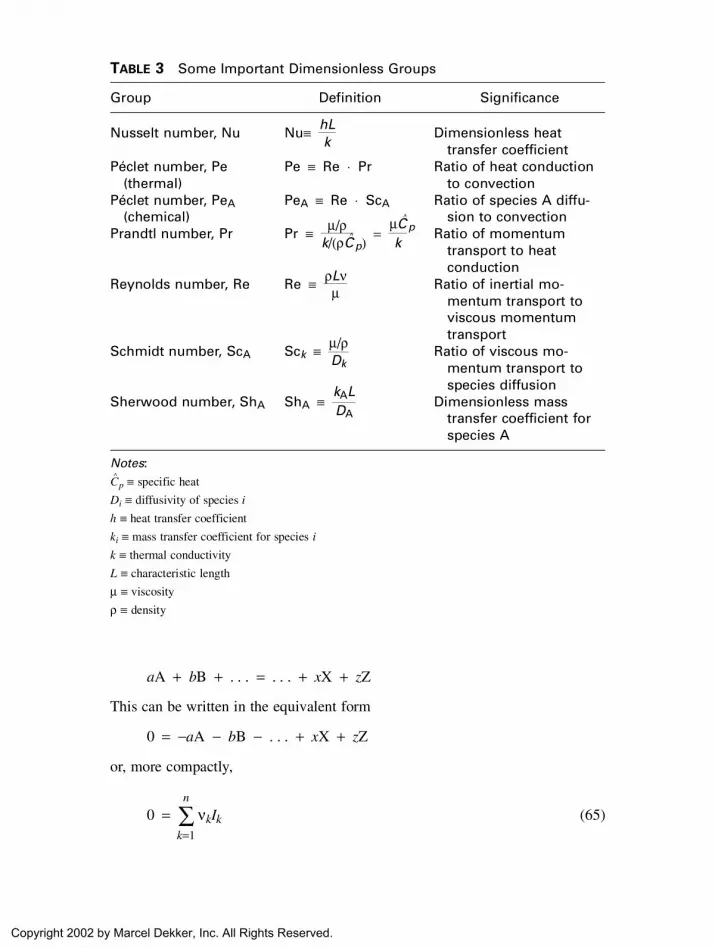
Heat and mass transfer coefficients are determined experimentally; theresults of such experiments are typically presented in terms of dimensionlessparameters. Table 3 lists a number of important dimensionless parameters. Thus,heat transfer data are often presented in terms of the Nusselt number, Nu, adimensionless heat transfer coefficient. In many cases, the Nusselt number isfound to be a function of the Reynolds number Re and the Prandtl number Pr:

Nu = ƒ(Re,Pr) (63)

The equivalent relation for mass transfer is

Sh = ƒ(Re,Sc) (64)

where Sh is the Sherwood number and Sc is the Schmidt number (see Table 3).Many standard handbooks and heat transfer textbooks list dimensionless transportrelationships for engineering systems (9,10).

4 STOICHIOMETRY AND CHEMICAL KINETICS

Stoichiometry is the study of the proportions in which elements combine to formcompounds. Chemical kinetics is the science dealing with the rates of chemicalreactions.

4.1 Stoichiometry

Consider a general chemical reaction in which reactants A, B, . . . react to formproducts X, Z, . . . according to the equation


aA + bB + . . . = . . . + xX + zZ

This can be written in the equivalent form

0 = −aA − bB − . . . + xX + zZ

or, more compactly,

0 = ∑k=1

n

νkIk (65)

TABLE 3 Some Important Dimensionless Groups

Group Definition Significance

Nusselt number, Nu Nu≡ hLk

Dimensionless heattransfer coefficient

Péclet number, Pe(thermal)

Pe ≡ Re ⋅ Pr Ratio of heat conductionto convection

Péclet number, PeA(chemical)

PeA ≡ Re ⋅ ScA Ratio of species A diffu-sion to convection

Prandtl number, Pr Pr ≡ µ/ρk/(ρC

^p)

=µC

^p

kRatio of momentum

transport to heatconduction

Reynolds number, Re Re ≡ ρLνµ Ratio of inertial mo-

mentum transport toviscous momentumtransport

Schmidt number, ScA Sck ≡ µ/ρDk

Ratio of viscous mo-mentum transport tospecies diffusion

Sherwood number, ShA ShA ≡kALDA

Dimensionless masstransfer coefficient forspecies A

Notes:

C^

p ≡ specific heat

Di ≡ diffusivity of species i

h ≡ heat transfer coefficient

ki ≡ mass transfer coefficient for species i

k ≡ thermal conductivity

L ≡ characteristic length

µ ≡ viscosity

ρ ≡ density


where νk is the stoichiometric coefficient of species Ik. Note that the stoichio-metric coefficient is positive for a product and negative for a reactant.

4.2 Reaction Rate

The rate of a chemical reaction can be defined in terms of the stoichiometriccoefficient:

ξ⋅

=(N⋅

A)gen

νA =

(N⋅B)gen

νB = . . . =

(N⋅k)gen

νk = . . . =

(N⋅X)gen

νX =

(N⋅Z)gen

νZ (66)

Here, ξ is the extent of reaction variable or reaction coordinate. The volumetricreaction rate r may be defined by:

r = ξ⋅

V(67)

The volumetric reaction rate is usually a function of the temperature andthe concentrations of the various reactants and products:

r = ±k(T)ƒ(cA,cB, . . . ,cX,cZ) (68)

where k(T) is the so-called rate constant (which is not really a constant, but ratheris a function of temperature).

In most cases, the rate constant is given by the Arrhenius equation:

k = k0 exp

−Ea

RT

(69)

In this equation, k0 is the preexponential factor and Ea is the activation energy,both of which must be determined experimentally.

The concentration-dependent part of the rate expression, ƒ(cA,cB, . . . , cX,cZ, must also be determined experimentally. In many cases, the reaction rate isfound to depend on the concentrations of the reacting species as follows:

ƒ(cA,cB, . . .) = cαAcβ

B . . . (70)

A reaction that obeys this equation is said to be of “α order” in species A, of “βorder” in species B, and so on. The overall order of the reaction n is the sum ofthe individual reaction orders:

n = α + β + . . . (71)

More information on the determination of rate constants and their applica-tions can be found in standard texts on kinetics and reactor design (6–8).


5 EQUILIBRIUM THERMODYNAMICS

Thermodynamics is the study of the relationship between heat, work, and variousforms of energy. Of particular interest to thermodynamics are the conditions forequilibrium.

5.1 Auxiliary Thermodynamic Functions

In addition to the energy and entropy, it is common in thermodynamics to definecertain auxiliary functions. One of these is the enthalpy or heat function H:

H = U + PV (72)

Two common free-energy functions are defined. The Helmholtz free-energyfunction A is defined by

A = U − TS (73)

The Gibbs free-energy function G is defined by

G = H − TS (74)

The Gibbs free-energy function is of special interest because it provides aconvenient criterion of spontaneity and equilibrium.

5.2 Spontaneity and Equilibrium

A spontaneous process is one that occurs in a closed system without the assistanceof some external agency. The Gibbs free energy decreases in a spontaneousprocess:

∆G ≤ 0 (spontaneous process) (75)

At equilibrium, the system does not change with time. The Gibbs free energyreaches a minimum at equilibrium:

dGdt

= 0 (equilibrium) (76)

5.3 Fugacity

The change in Gibbs free energy for an ideal gas undergoing an isothermalcompression or expansion from pressure P1 to pressure P2 is given by

∆G = RT ln P2

P1 (ideal gas) (77)

Although Eq. (77) does not apply for a real gas, it is common practice to retainthe same functional form for real gases:


∆G = RT ln ƒ2

ƒ1 (real gas) (78)

Here, ƒ1 is the fugacity at pressure P1. The fugacity may be considered as anadjusted pressure. It is defined so as to coincide with the pressure at low densities:

limP→0

ƒP

= 1 (79)

The ratio of fugacity to pressure is called the fugacity coefficient, φ. Thus, theprevious equation may be written

ϕ ≡ ƒP

⇒ limP→0

ϕ = 1 (80)

5.4 Chemical Potential

Consider a solution consisting of n species A, B, . . . . The Gibbs free energy ofthe solution is given by

G = ∑k=1

n

Nkµk (81)

where µk is the chemical potential of species k, defined by

µk =

∂G∂Nk

T,P,Nj≠k

(82)

5.5 Fugacity and Activity

The chemical potential is generally a function of temperature, pressure, andcomposition. It is common practice to write

µA = µ˚A(T) + RT ln aA (83)

where µ˚A(T) is the standard chemical potential and aA is the activity of speciesA. The activity is defined as the ratio of the fugacity ƒA to a standard-statefugacity ƒ˚A:

aA =ƒA

ƒ˚A(84)

Activities and standard states are discussed in greater detail in many texts onchemical thermodynamics (11,12).


5.6 Phase Equilibrium

Consider a multicomponent system that separates into two or more phases(denoted I, II, . . .). The criteria for phase equilibrium are

TI = TII = . . . (thermal equilibrium) (85)

PI = PII = . . . (mechanical equilibrium) (86)

(µA)I = (µA)II = . . . (equilibrium for species A) (87)

(µB)I = (µB)II = . . . (equilibrium for species B) (88)

...

5.7 Reaction Equilibrium

Consider a reaction

aA + bB + . . . = . . . + xX + zZ

which, as before, can be expressed in the shorthand notation

0 = ∑k=1

n

νkIk

The criterion for chemical reaction equilibrium is

∆G = ∑k=1

n

νkµk = 0 (89)

Reaction equilibrium may also be expressed in terms of the standard Gibbsfree-energy change:

∆G0 = RT ln Ka (90)

Here, Ka is the equilibrium constant, defined by

Ka = ∏k=1

n

akνk (91)

6 ENGINEERING FLUID MECHANICS

Fluid mechanics deals with the flow of liquids and gases. For most engineeringapplications, a macroscopic approach is usually taken.


6.1 Engineering Bernoulli Equation

Most engineering problems in fluid mechanics can be solved using the engineer-ing Bernoulli equation, also called the mechanical energy balance. It can bederived from the macroscopic energy balance (see Ref. 13), subject to thefollowing restrictions: (a) the system is at steady state; (b) the system has a singlefluid intake and a single outlet; (c) gravity is the sole body force, with constant|g|; (d) the flow is incompressible; (e) the system may include one or more pumpsor turbines. Under these conditions, the macroscopic energy balance becomes

∆ Pρ + |g|z + α

2⟨ν⟩2

=W

⋅s

m⋅ − F⋅

m⋅ (92)

where

P = the fluid pressure

⟨ν⟩ = the velocity averaged over the cross section of the pipe or conduit

α = average velocity correction factor (2.0 for laminar flow and 1.07 forturbulent flow)

W⋅

2 = rate of work done by pumps or turbines (positive for pumps,negative for turbines)

F⋅ = frictional loss rate

Dividing by the acceleration of gravity |g| yields the so-called head form of theBernoulli equation:

∆

Pρ|g|

+ z + α2|g|

⟨ν⟩2

=W

⋅s

m⋅ |g|− F

⋅ m⋅ |g|

(93)

Each of the terms in this equation has the dimensions of length.

6.2 Fluid Friction in Pipes and Conduits

The frictional loss rate F⋅ equals the rate at which useful mechanical energy isconverted to thermal energy by friction. It is usually computed from an equationof the form

F⋅

m⋅ = 4ƒ

LD

⟨ν⟩2

2(94)

where ƒ is the Fanning friction factor.* In general, the friction factor is a function

*This is not the only friction factor in widespread use. Some authors prefer the Darcy-Wiessbachfriction factor, ƒDW = 4ƒ.


of the pipe diameter D, the surface roughness ε, and the Reynolds number Re,the latter being defined as

Re = ρD|ν|µ (95)

where µ is the fluid viscosity.In the laminar-flow regime, ƒ = 16/Re. For turbulent flows, a number of

charts, graphs, and equations are available to compute the friction factor. TheColebrook equation has traditionally been used, although it requires a trial-and-error solution to find ƒ:

1√ƒ = −4 log

ε/D3.7

+ 1.255Re√ƒ

(96)

Wood’s approximation (Ref. 13) gives ƒ directly, without a trial-and-errorprocedure:

ƒ = a + b Re−c (97)

where

a = 0.0235

εD

0.225

+ 0.1325

εD

(98)

b = 22

εD

0.44

(99)

c = 1.62

εD

0.134

(100)

The relations presented in this section were developed for cylindrical pipes ortubes; however, the same equations may be used for noncylindrical ducts if thepipe diameter D is replaced in Eqs. (94–100) by the hydraulic diameter DH:

DH = 4 volume of fluid

area wetted by fluid(101)

6.3 Minor Losses

The relations developed in the previous section apply only to straight pipes orconduits. Most pipelines, however, include bends, valves, and other fittings whichcreate additional frictional losses. These additional losses are often called “minorlosses,” although they may actually exceed the friction caused by the pipe itself.

There are two common ways to account for minor losses. One is to definean equivalent length Leq which equals the length of straight pipe that would givethe same frictional loss as the valve or fitting in question. The total equivalent


length Ltotal is the sum of the true length of the pipe and the individual equivalentlengths of the valves and fitting:

Ltotal = Lpipe + ∑fitting i

(Leq)i (102)

The total equivalent length Ltotal is used in Eq. (94) in place of L to compute thetotal frictional losses.

The second common approach to computing minor losses relies on theconcept of a loss coefficient KL, defined for each type of valve or fitting accordingto the equation

F⋅

m⋅ = KL⟨ν⟩2

2(103)

A comprehensive listing of typical equivalent lengths and loss coefficients ispublished by the Crane Company (14).

6.4 Fluid Friction in Porous Media

A porous medium is a solid material containing voids through which fluids mayflow. The most important single parameter used to described porous media is theporosity or void fraction ε:

ε = void volumebulk volume

=Vvoids

Vvoids + Vsolid(104)

Fluid friction in a porous medium of thickness L is usually described by Darcy’s law:

F⋅

m⋅ = µρ

Lk

⟨ν⟩ (105)

where k is a material property called the permeability.

REFERENCES

1. R. B. Bird, W. E. Stewart, and E. N. Lightfoot, Transport Phenomena. New York:Wiley, 1960.

2. M. M. Denn, Process Fluid Mechanics. Englewood Cliffs, NJ: Prentice-Hall, 1980. 3. R. W. Fahien, Fundamentals of Transport Phenomena. New York: McGraw-Hill,

1983. 4. W. M. Deen, Analysis of Transport Phenomena. New York: Oxford University Press,

1998. 5. E. L. Cussler, Diffusion Mass Transfer in Fluid Systems, 2nd ed. Cambridge, U.K.:

Cambridge University Press, 1997.


6. O. Levenspiel, Chemical Reaction Engineering, 2nd ed. New York: Wiley, 1972. 7. H. S. Fogler, Elements of Chemical Reaction Engineering. Englewood Cliffs, NJ:

PTR Prentice-Hall, 1992. 8. L. D. Schmidt, The Engineering of Chemical Reactions. New York: Oxford Univer-

sity Press, 1998. 9. F. P. Incropera and D. P. DeWitt, Fundamentals of Heat and Mass Transfer, 3rd ed.

New York: Wiley, 1990.10. D. R. Lide (ed.), CRC Handbook of Chemistry and Physics, 80th ed. Cleveland, OH:

CRC Press, 1999.11. I. M. Klotz and R. M. Rosenberg. Chemical Thermodynamics: Basic Theory and

Methods, 3rd ed. Menlo Park, CA: W. A. Benjamin, 1972.12. K. Denbigh, The Principles of Chemical Equilibrium, 3rd ed. Cambridge, U.K.:

Cambridge University Press, 1971.13. N. De Nevers, Fluid Mechanics for Chemical Engineers, 2nd ed. New York:

McGraw-Hill, 1991.14. Flow of Fluids Through Valves, Fittings, and Pipe, Crane Technical Paper 410.

Chicago: The Crane Company, 1988.


Documents

Macroscopic Balance Equations