1

Paper to be presented at Americas User Conference, Oct 5-9,Sheraton Universal Hotel, Universal City, California

Title: Finite Element Based Fatigue Analysis

Authors: Dr NWM Bishop, MSC Frimley and Alan Caserio. MSC Costa Mesa

Abstract

Fatigue analysis procedures for the design of modern structures rely on techniques, which have been developed overthe last 100 years or so. The first accepted technique was the S-N or stress-life method generally given credit to theGerman August Woehler for his systematic tests done on railway axles in the 1870’s. Initially these techniques wererelatively simple procedures, which compared measured constant amplitude stresses (from prototype tests) withmaterial data from test coupons. These techniques have become progressively more sophisticated with theintroduction of strain based techniques to deal with local plasticity effects. Nowadays, variable stress responses canbe dealt with. Furthermore, techniques exist to predict how fast a crack will grow through a component, instead ofthe more limited capability to simply predict the time to failure. Even more recently techniques have beenintroduced to deal with the occurrence of stresses in more than one principal direction (multi-axial fatigue) and todeal with vibrating structures where responses are predicted as PSD’s (Power Spectral Density’s) of stress. Evenmore recently researchers have addressed the requirements for the design of specific components such as spot welds.All of these techniques were developed outside of the Finite Element environment. However, they have now beenimplanted into many FE based analysis programs, the best known of which is MSCFATIGUE. The FE environmentintroduces additional considerations relating to how input data is processed and how fatigue life, or damage, resultsare post processed. This paper will deal with the issues associated with how fatigue techniques can be incorporatedinto the FE environment. Modern examples of FE based fatigue design will be included.

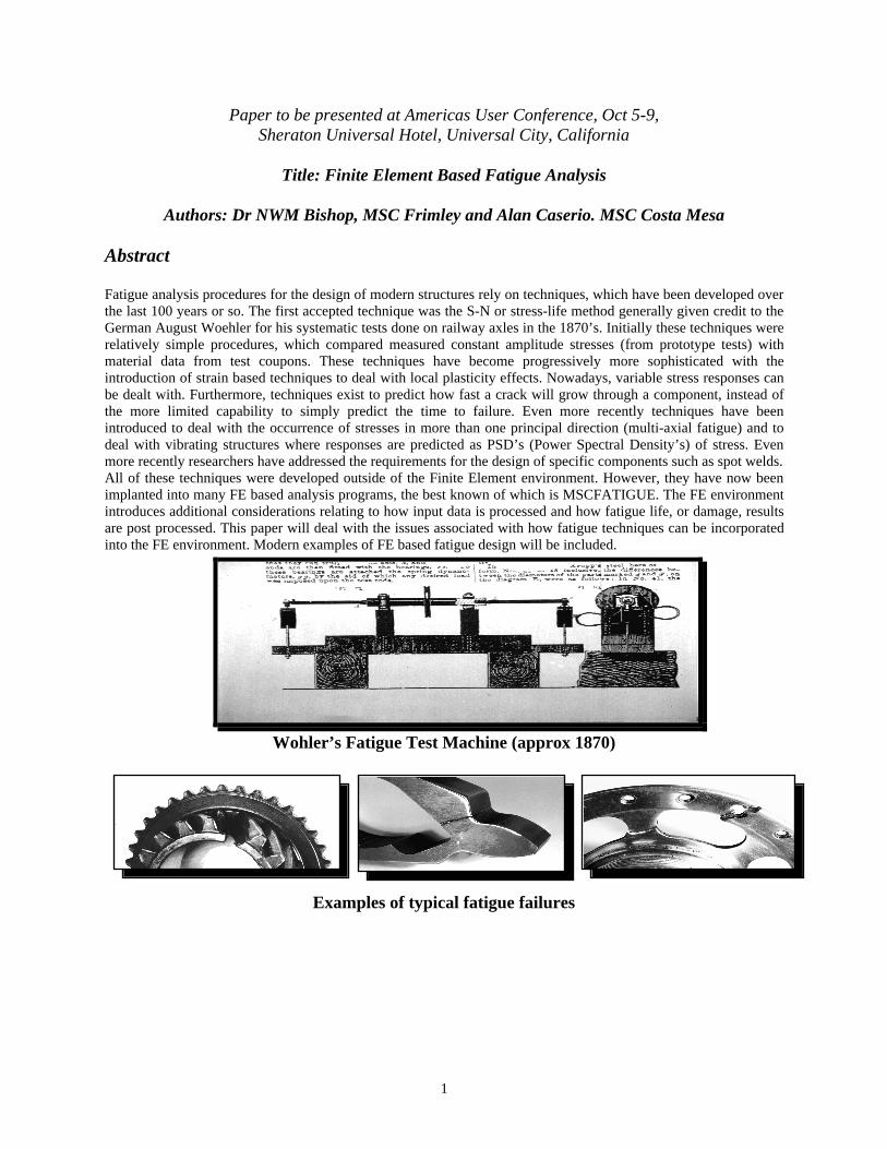
Wohler’s Fatigue Test Machine (approx 1870)

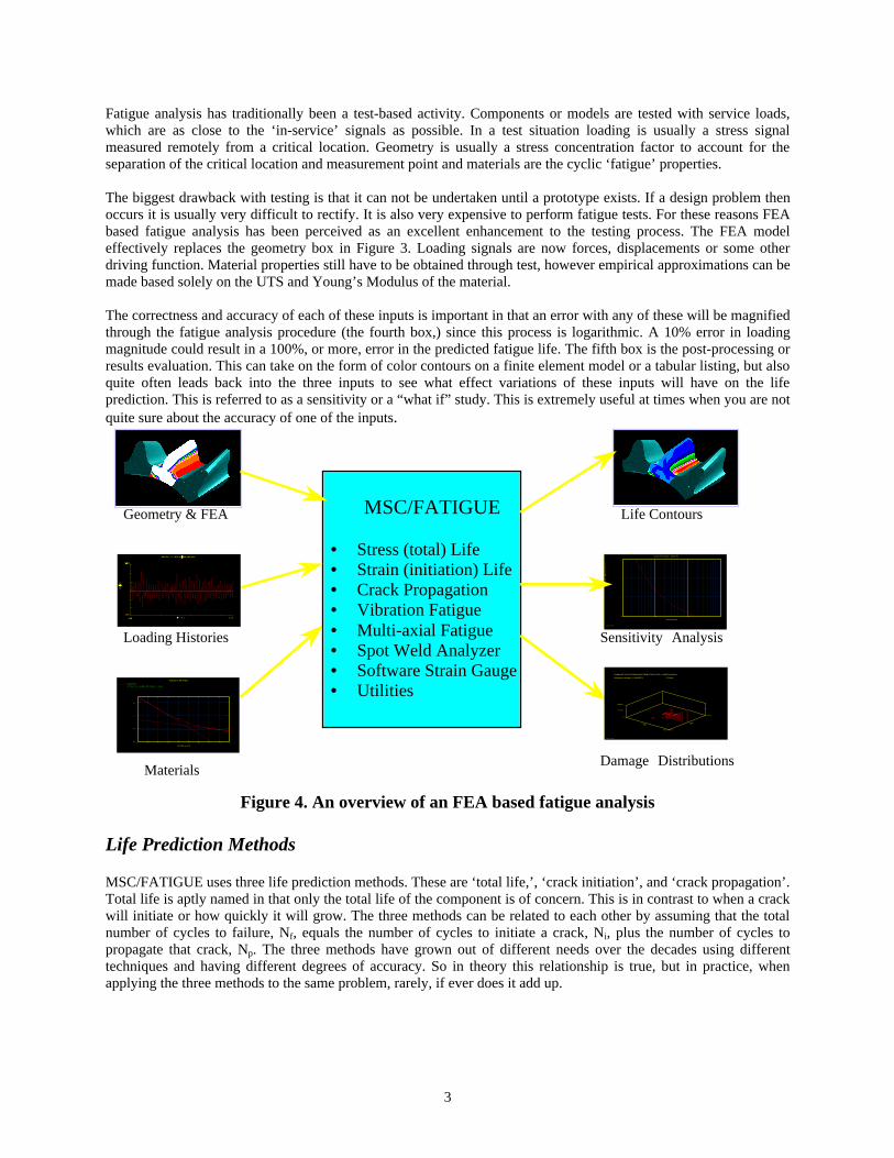
Examples of typical fatigue failures

2

Introduction and Background

MSC/FATIGUE is an advanced fatigue life estimation program for use with finite element analysis. When usedearly in a development design cycle it is possible to greatly enhance product life as well as reduce testing andprototype costs thus ensuring greater speed to market.

However, before describing the features of the product in detail it isuseful to define the term fatigue. Very often the terms fatigue, fracture,and durability are used interchangeably. Each does however convey aspecific meaning. Although many definitions can be applied to the word,for the purposes of this paper, fatigue is failure under a repeated orotherwise varying load which never reaches a level sufficient to causefailure in a single application. It can also be thought of as the initiationand growth of a crack, or growth from a pre-existing defect, until itreaches a critical size, such as separation into two or more parts.

Fatigue analysis itself usually refers to one of two methodologies. Thestress-life (or S-N method), is commonly referred to as the total lifemethod since it makes no distinction between initiating or growing acrack. This was the first fatigue analysis method to be developed over100 years ago. The local-strain or strain-life (_-N) method, commonlyreferred to as the crack initiation method, was more recently developedand concerns itself only with the ‘initiation’ of a crack.

Fracture specifically concerns itself with the growth or propagation of acrack once it has initiated and this has given rise to many so-called crackgrowth methodologies.

Figure 1. The FEA fatigueenvironment

Figure 2. Fatigue or crackpropagation?

Durability is then the conglomeration of all aspects that effect the life of a product and usually involves much morethan just fatigue and fracture, but also loading conditions, environmental concerns, material characterizations, andtesting simulations to name a few. A true product durability program in an organization takes all of these aspects(and more) into consideration.

Why FEA based fatigue analysis?

All fatigue analysis calculations are performed within theconstraints of the so-called ‘five-box trick.’ The illustrationbelow shows how this concept can be visualized. For any lifeanalysis, whether it be fatigue or fracture, there are always threeinputs. The first three boxes are these inputs:

Materials

Loading

Geometry

Analysis Results

Figure 3. The ‘fatigue’ 5 box trick

3

Fatigue analysis has traditionally been a test-based activity. Components or models are tested with service loads,which are as close to the ‘in-service’ signals as possible. In a test situation loading is usually a stress signalmeasured remotely from a critical location. Geometry is usually a stress concentration factor to account for theseparation of the critical location and measurement point and materials are the cyclic ‘fatigue’ properties.

The biggest drawback with testing is that it can not be undertaken until a prototype exists. If a design problem thenoccurs it is usually very difficult to rectify. It is also very expensive to perform fatigue tests. For these reasons FEAbased fatigue analysis has been perceived as an excellent enhancement to the testing process. The FEA modeleffectively replaces the geometry box in Figure 3. Loading signals are now forces, displacements or some otherdriving function. Material properties still have to be obtained through test, however empirical approximations can bemade based solely on the UTS and Young’s Modulus of the material.

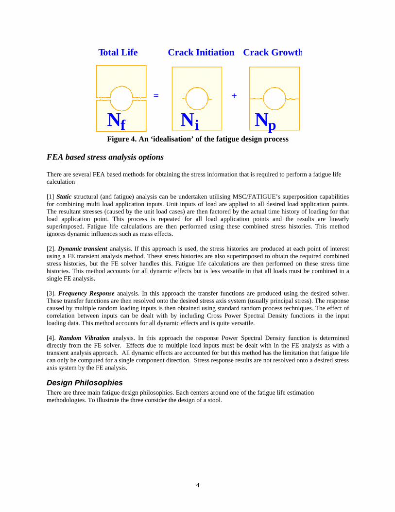
The correctness and accuracy of each of these inputs is important in that an error with any of these will be magnifiedthrough the fatigue analysis procedure (the fourth box,) since this process is logarithmic. A 10% error in loadingmagnitude could result in a 100%, or more, error in the predicted fatigue life. The fifth box is the post-processing orresults evaluation. This can take on the form of color contours on a finite element model or a tabular listing, but alsoquite often leads back into the three inputs to see what effect variations of these inputs will have on the lifeprediction. This is referred to as a sensitivity or a “what if” study. This is extremely useful at times when you are notquite sure about the accuracy of one of the inputs.

Figure 4. An overview of an FEA based fatigue analysis

Life Prediction Methods

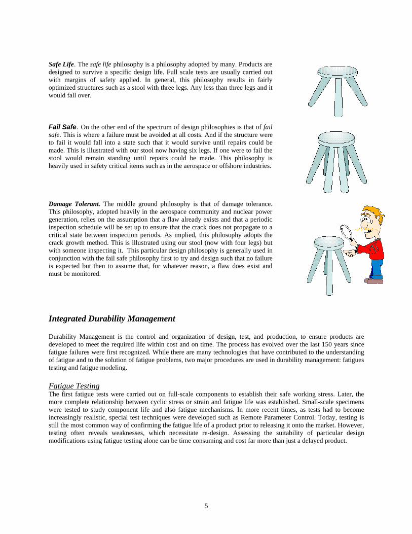
MSC/FATIGUE uses three life prediction methods. These are ‘total life,’, ‘crack initiation’, and ‘crack propagation’.Total life is aptly named in that only the total life of the component is of concern. This is in contrast to when a crackwill initiate or how quickly it will grow. The three methods can be related to each other by assuming that the totalnumber of cycles to failure, Nf, equals the number of cycles to initiate a crack, Ni, plus the number of cycles topropagate that crack, Np. The three methods have grown out of different needs over the decades using differenttechniques and having different degrees of accuracy. So in theory this relationship is true, but in practice, whenapplying the three methods to the same problem, rarely, if ever does it add up.

Geometry & FEA

Loading Histories

Materials

InforInfor

Damage Distributions

Life Contours

Sensitivity Analysis

Strain Life Plot

MANTEN

Sf': 917 b: -0.095 Ef': 0.26 c: -0.47

1E-4

1E-3

1E-2

1E-1

1E0 1E1 1E2 1E3 1E4 1E5 1E6 1E7 1E8 1E9

Life (Reversals)

nCode nSoft

0

5281.3-1732.5

3496.50

6.8848E-5

RangeuE

MeanuE

Damage

DAMAGE HISTOGRAM DISTRIBUTION FOR : SAETRN.DHH

Maximum height : 6.8848E-5 Z Units :

nCode nSoft

1E2 1E3 1E42

3

4

5

Cross Plot of Data : SAETRN

Life(Repeats)

Scale Factor( )

MSC/FATIGUE

• Stress (total) Life• Strain (initiation) Life• Crack Propagation• Vibration Fatigue• Multi-axial Fatigue• Spot Weld Analyzer• Software Strain Gauge• Utilities

4

Total Life Crack Initiation Crack Growth

= +

Ni Nf Np Figure 4. An ‘idealisation’ of the fatigue design process

FEA based stress analysis options

There are several FEA based methods for obtaining the stress information that is required to perform a fatigue lifecalculation

[1] Static structural (and fatigue) analysis can be undertaken utilising MSC/FATIGUE’s superposition capabilitiesfor combining multi load application inputs. Unit inputs of load are applied to all desired load application points.The resultant stresses (caused by the unit load cases) are then factored by the actual time history of loading for thatload application point. This process is repeated for all load application points and the results are linearlysuperimposed. Fatigue life calculations are then performed using these combined stress histories. This methodignores dynamic influences such as mass effects.

[2]. Dynamic transient analysis. If this approach is used, the stress histories are produced at each point of interestusing a FE transient analysis method. These stress histories are also superimposed to obtain the required combinedstress histories, but the FE solver handles this. Fatigue life calculations are then performed on these stress timehistories. This method accounts for all dynamic effects but is less versatile in that all loads must be combined in asingle FE analysis.

[3]. Frequency Response analysis. In this approach the transfer functions are produced using the desired solver.These transfer functions are then resolved onto the desired stress axis system (usually principal stress). The responsecaused by multiple random loading inputs is then obtained using standard random process techniques. The effect ofcorrelation between inputs can be dealt with by including Cross Power Spectral Density functions in the inputloading data. This method accounts for all dynamic effects and is quite versatile.

[4]. Random Vibration analysis. In this approach the response Power Spectral Density function is determineddirectly from the FE solver. Effects due to multiple load inputs must be dealt with in the FE analysis as with atransient analysis approach. All dynamic effects are accounted for but this method has the limitation that fatigue lifecan only be computed for a single component direction. Stress response results are not resolved onto a desired stressaxis system by the FE analysis.

Design PhilosophiesThere are three main fatigue design philosophies. Each centers around one of the fatigue life estimationmethodologies. To illustrate the three consider the design of a stool.

5

Safe Life. The safe life philosophy is a philosophy adopted by many. Products aredesigned to survive a specific design life. Full scale tests are usually carried outwith margins of safety applied. In general, this philosophy results in fairlyoptimized structures such as a stool with three legs. Any less than three legs and itwould fall over.

Fail Safe. On the other end of the spectrum of design philosophies is that of failsafe. This is where a failure must be avoided at all costs. And if the structure wereto fail it would fall into a state such that it would survive until repairs could bemade. This is illustrated with our stool now having six legs. If one were to fail thestool would remain standing until repairs could be made. This philosophy isheavily used in safety critical items such as in the aerospace or offshore industries.

Damage Tolerant. The middle ground philosophy is that of damage tolerance.This philosophy, adopted heavily in the aerospace community and nuclear powergeneration, relies on the assumption that a flaw already exists and that a periodicinspection schedule will be set up to ensure that the crack does not propagate to acritical state between inspection periods. As implied, this philosophy adopts thecrack growth method. This is illustrated using our stool (now with four legs) butwith someone inspecting it. This particular design philosophy is generally used inconjunction with the fail safe philosophy first to try and design such that no failureis expected but then to assume that, for whatever reason, a flaw does exist andmust be monitored.

Integrated Durability Management

Durability Management is the control and organization of design, test, and production, to ensure products aredeveloped to meet the required life within cost and on time. The process has evolved over the last 150 years sincefatigue failures were first recognized. While there are many technologies that have contributed to the understandingof fatigue and to the solution of fatigue problems, two major procedures are used in durability management: fatiguestesting and fatigue modeling.

Fatigue TestingThe first fatigue tests were carried out on full-scale components to establish their safe working stress. Later, themore complete relationship between cyclic stress or strain and fatigue life was established. Small-scale specimenswere tested to study component life and also fatigue mechanisms. In more recent times, as tests had to becomeincreasingly realistic, special test techniques were developed such as Remote Parameter Control. Today, testing isstill the most common way of confirming the fatigue life of a product prior to releasing it onto the market. However,testing often reveals weaknesses, which necessitate re-design. Assessing the suitability of particular designmodifications using fatigue testing alone can be time consuming and cost far more than just a delayed product.

6

Fatigue ModelingThe estimation of fatigue life using mathematical modeling techniques was developed to assist the engineer insolving fatigue problems without always having to physically test all the options. For this reason, techniques such aslocal strain or crack initiation modeling have become widely used. Improvements in the power of computers haveenabled the effective use of these techniques. Today, most major companies designing mechanical structures willuse a fatigue life estimation tool such as MSC/FATIGUE in conjunction with testing. The late 1980s had establishthe use of finite element analysis (FEA) as a tool for stress analysis. At the same time the integration of FEA andfatigue life estimation through the MSC/FATIGUE product began to provide new benefits by assessing fatigueearlier in the development process.

Integrated Durability ManagementUnderstanding and effective implementation of durability management strategies requires a partnership between testand design analysis. It can reduce product lead-time by focussing the use of fatigue testing to the essentialcorrelation and sign-off tests. The use of fatigue modeling, at the design analysis stage, allows more options to beassessed for little incremental cost. Integrated durability management can produce better products more quickly andcheaply.

Components of MSC/FATIGUE. Stress – Life and Strain – Life Analysis

The stress–life and strain–life methods are the most common forms of fatigue life prediction. They both involvestress cycle counting, using, for instance rainflow cycle counting. Many materials data curve corrections areavailable to deal with surface finish, surface treatment, mean stresses and elastic – plastic corrections (for strain –life approach). Damage is assessed through a materials look up curve, either S-N or E-N and damage is summedusing the conventional Palmgren Miner cumulative damage hypothesis.

The total life method, more commonly known as the stress-life or S-N method, typically makes no distinctionbetween initiating or growing a crack, but rather, predicts the total life to catastrophic failure. Total life specificfeatures include:

• Goodman or Gerber mean stress correction• Welded structure analysis to BS7608• Material and component S-N curves

Sophisticated crack initiation or strain-life (ε-N) modeling provides a method for estimating life to the initiation ofan engineering crack. Crack initiation specific features include:

• Neuber elastic-plastic correction.• Advanced elastic-plastic correction based on Mertens-Dittman or Seeger-Beste methods• Cyclic stress-strain tracking using Massing’s hypothesis and material memory modeling• Smith-Watson-Topper and Morrow mean stress correction• Advanced biaxial corrections (proportional loading) based on Parameter Modification or Hoffman-Seeger

Components of MSC/FATIGUE - Crack Propagation Analysis

For all fatigue and fracture analyses we require the three major inputs: geometry, materials, and loading. This is nodifferent for a Crack Growth analysis except that geometry definition takes on a different form. The onlyinformation necessary for this approach is the remote stress used in the Paris Equation and a description of thestress intensity.

7

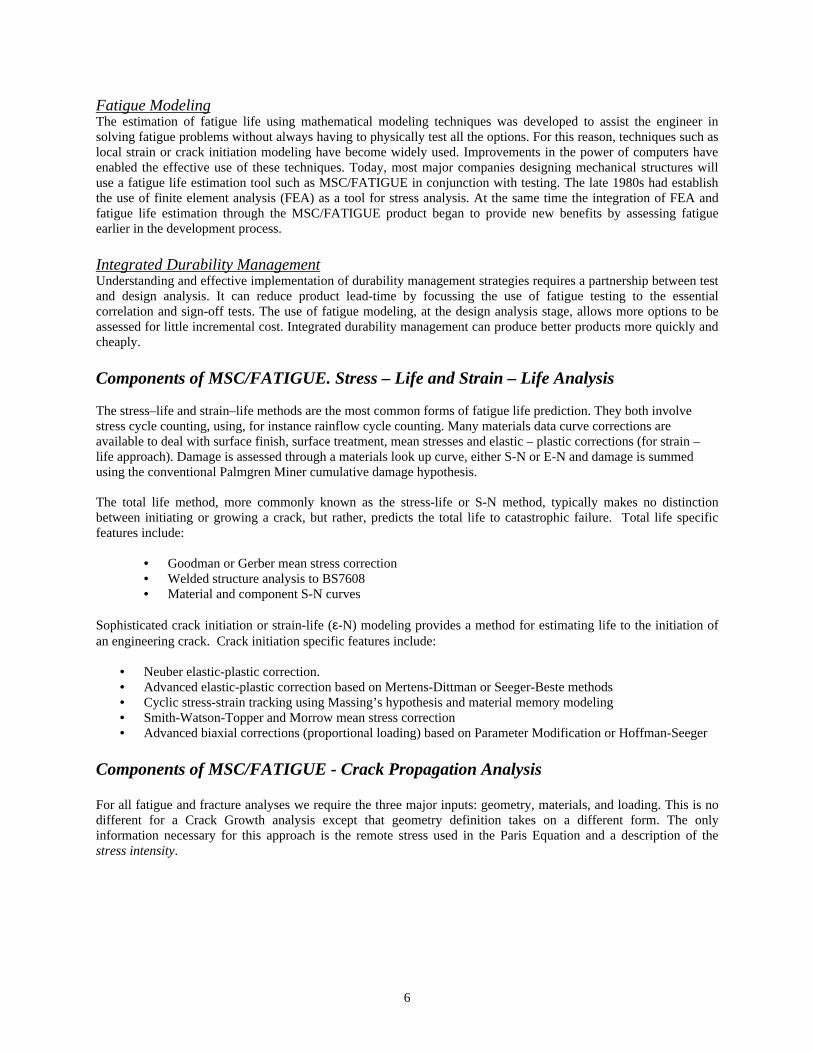
When a notch becomes a crack, the stress field becomes a singularity (in theoretical elastic terms) and the stressconcentration, K t, is no longer a useful way of describing the feature. Rather we need something that describes theintensity of the stress field around the singularity. This concept is well illustrated by the diagram below where a holeis introduced into an infinite plate. As the hole becomes an ellipse and the ratio of the length to width of the ellipsebecomes greater and greater, tending towards infinity, so does the stress concentration.

Figure 5. The concept of stress intensity

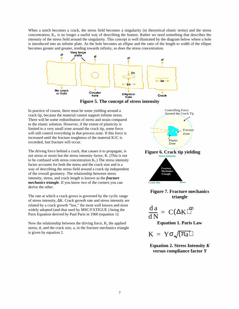
In practice of course, there must be some yielding around acrack tip, because the material cannot support infinite stress.There will be some redistribution of stress and strain comparedto the elastic solution. However, if the extent of plasticity islimited to a very small zone around the crack tip, some forcewill still control everything in that process zone. If this force isincreased until the fracture toughness of the material K1C isexceeded, fast fracture will occur.

The driving force behind a crack, that causes it to propagate, isnot stress or strain but the stress intensity factor, K. (This is notto be confused with stress concentration Kt.) The stress intensityfactor accounts for both the stress and the crack size and is away of describing the stress field around a crack tip independentof the overall geometry. The relationship between stressintensity, stress, and crack length is known as the fracturemechanics triangle. If you know two of the corners you canderive the other.

The rate at which a crack grows is governed by the cyclic rangeof stress intensity, ∆K. Crack growth rate and stress intensity arerelated by a crack growth “law,” the most well known and mostwidely adopted (and that used by MSC/FATIGUE ) being theParis Equation derived by Paul Paris in 1960 (equation 1):

Now the relationship between the driving force, K, the appliedstress, σ, and the crack size, a, in the fracture mechanics triangleis given by equation 2.

FractureZone

PlasticZone

Controlling ForceAround the Crack Tip

Figure 6. Crack tip yieldingStress Intensity

StressCrack Size

FractureMechanicsTriangle

Figure 7. Fracture mechanicstriangle

d ad N------- C ∆K( )m

=

Equation 1. Paris Law

K Yσ πa( )=

Equation 2. Stress Intensity Kversus compliance factor Y

8

Y is known as the compliance function and describes the geometry in which the crack exists. It relates crack lengthto geometric features of the part or component. Perhaps one way to describe a compliance function in physical termsis the change in stiffness or flexibility (compliance) as the crack grows, i.e., the structure becomes more compliantas the crack gets longer. The dictionary defines compliant as ready or disposed to comply, and compliance as the actor process of complying to a desire, demand, or proposal or to coercion. In engineering terms it is the ability of anobject to yield when a force is applied.

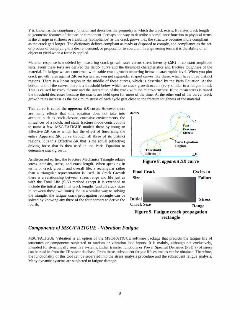
Material response is modeled by measuring crack growth rates versus stress intensity (∆K) in constant amplitudetests. From these tests are derived the da/dN curve and the threshold characteristics and fracture toughness of thematerial. In fatigue we are concerned with stable crack growth occurring below a catastrophic level. When you plotcrack growth rates against ∆K on log scales, you get sigmoidal shaped curves like these, which have three distinctregions. There is a linear region in the middle of these curves, which is described by the Paris Equation. At thebottom end of the curves there is a threshold below which no crack growth occurs (very similar to a fatigue limit).This is caused by crack closure and the interaction of the crack with the micro-structure. If the mean stress is raisedthe threshold decreases because the cracks are held open for more of the time. At the other end of the curve, crackgrowth rates increase as the maximum stress of each cycle gets close to the fracture toughness of the material.

This curve is called the apparent ∆K curve. However thereare many effects that this equation does not take intoaccount, such as crack closure, corrosive environments, theinfluences of a notch, and static fracture mode contributionsto name a few. MSC/FATIGUE models these by using anEffective ∆K curve which has the effect of linearizing theentire Apparent ∆K curve through all three of its distinctregions. It is this Effective ∆K that is the actual (effective)driving force that is then used in the Paris Equation todetermine crack growth.

As discussed earlier, the Fracture Mechanics Triangle relatesstress intensity, stress, and crack length. When speaking interms of crack growth and overall life, a rectangular ratherthan a triangular representation is used. In Crack Growththere is a relationship between stress range and life just aswith the Total Life (S-N) method except it is extended toinclude the initial and final crack lengths (and all crack sizesin-between these two limits). So in a similar way to solvingthe triangle, the fatigue crack propagation rectangle can besolved by knowing any three of the four corners to derive thefourth.

ThresholdEffects

FastFractureEffects

Paris EquationRegion

∆K

da/dN

Figure 8. apparent ∆K curve

Final CrackSize

InitialCrack Size

Cycles to Failure

Stress

Range

Figure 9. Fatigue crack propagationrectangle

Components of MSC/FATIGUE - Vibration Fatigue

MSC/FATIGUE Vibration is an option of the MSC/FATIGUE software package that predicts the fatigue life ofstructures or components subjected to random or vibration load inputs. It is mainly, although not exclusively,intended for dynamically sensitive systems. Either transfer functions or Power Spectral Densities (PSD’s) of stresscan be read in from the FE solver database. From these, subsequent fatigue life estimates can be obtained. Therefore,the functionality of this tool can be separated into the stress analysis procedure and the subsequent fatigue analysis.Many dynamic systems are subjected to fatigue damage.

9

Such systems are currently designed, and analyzed, predominantly through the use of expensive and time consumingtest based procedures. MSC/FATIGUE vibration allows designers to identify and deal with such damage at a muchearlier stage in the design process, thus reducing or eliminating the need for expensive prototype tests.

As well as a fatigue analyzer this module also contains a state of the art analysis tool which provides a completesolution path for multiple load case frequency domain based analysis. It includes new advances in stress tensormobility and biaxiality checking.

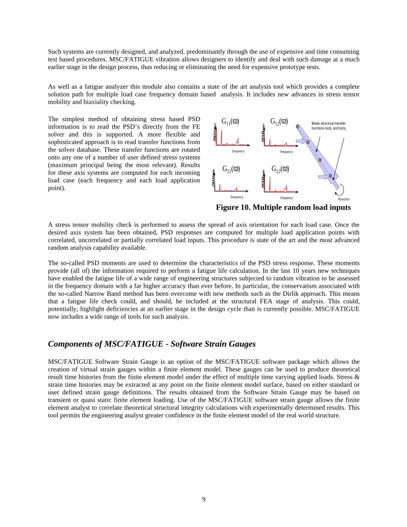
The simplest method of obtaining stress based PSDinformation is to read the PSD’s directly from the FEsolver and this is supported. A more flexible andsophisticated approach is to read transfer functions fromthe solver database. These transfer functions are rotatedonto any one of a number of user defined stress systems(maximum principal being the most relevant). Resultsfor these axis systems are computed for each incomingload case (each frequency and each load applicationpoint).

Blade structural transferfunctions h(ω)1 and h(ω)2

G11(ω) G12(ω)

G22(ω)G21(ω)

PS

D F

orc

e

frequency

PS

D F

orc

e

frequency

PS

D F

orc

e

frequency

PS

D F

orc

e

frequency Reaction

Figure 10. Multiple random load inputs

A stress tensor mobility check is performed to assess the spread of axis orientation for each load case. Once thedesired axis system has been obtained, PSD responses are computed for multiple load application points withcorrelated, uncorrelated or partially correlated load inputs. This procedure is state of the art and the most advancedrandom analysis capability available.

The so-called PSD moments are used to determine the characteristics of the PSD stress response. These momentsprovide (all of) the information required to perform a fatigue life calculation. In the last 10 years new techniqueshave enabled the fatigue life of a wide range of engineering structures subjected to random vibration to be assessedin the frequency domain with a far higher accuracy than ever before. In particular, the conservatism associated withthe so-called Narrow Band method has been overcome with new methods such as the Dirlik approach. This meansthat a fatigue life check could, and should, be included at the structural FEA stage of analysis. This could,potentially, highlight deficiencies at an earlier stage in the design cycle than is currently possible. MSC/FATIGUEnow includes a wide range of tools for such analysis.

Components of MSC/FATIGUE - Software Strain Gauges

MSC/FATIGUE Software Strain Gauge is an option of the MSC/FATIGUE software package which allows thecreation of virtual strain gauges within a finite element model. These gauges can be used to produce theoreticalresult time histories from the finite element model under the effect of multiple time varying applied loads. Stress &strain time histories may be extracted at any point on the finite element model surface, based on either standard oruser defined strain gauge definitions. The results obtained from the Software Strain Gauge may be based ontransient or quasi static finite element loading. Use of the MSC/FATIGUE software strain gauge allows the finiteelement analyst to correlate theoretical structural integrity calculations with experimentally determined results. Thistool permits the engineering analyst greater confidence in the finite element model of the real world structure.

10

The software strain gauges are defined as finite element groups, each containing between 1 to 3 elements. Allstandard strain gauge definitions are supported in both planar and stacked formulations. User defined gauges mayalso be created, with definitions stored in a gauge definition file.

The virtual strain gauges are positioned on the finite element model surface, with the gauge aligned in anyorientation, and the gauge covering multiple finite elements. The results obtained from the Software Strain Gaugeare averaged results from the underlying finite elements, modeling the same geometric averaging obtained withactual instrumentation. Results are transformed to the coordinate system and alignment of the software strain gauge.The Software Strain Gauge has the following features:

• Multiple Gauge Geometries• Uniaxial Gauges• T Gauges• Delta & Rectangular Gauges• Stacked & Planar Gauges• User Specified Gauge Definitions• Gauge Definition Files (user definable gauges)• Up to 200 simultaneous Software Strain Gauges

The Software Strain Gauge is also of benefit to the analyst performing MSC/FATIGUE weld durability calculationsin accordance with British Standard 7608. The Gauge tool allows ready access to strain time histories at the weldtoe, providing important information for weld durability calculations.

Components of MSC/FATIGUE - Spot Weld Analyser

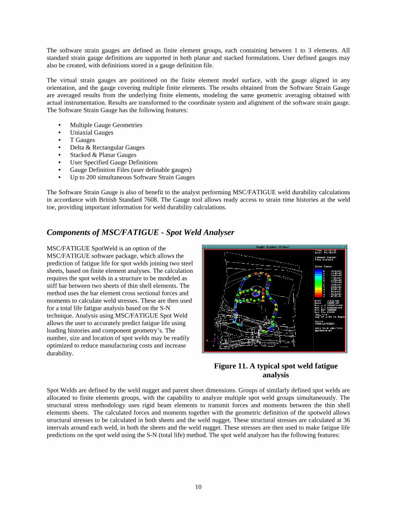
MSC/FATIGUE SpotWeld is an option of theMSC/FATIGUE software package, which allows theprediction of fatigue life for spot welds joining two steelsheets, based on finite element analyses. The calculationrequires the spot welds in a structure to be modeled asstiff bar between two sheets of thin shell elements. Themethod uses the bar element cross sectional forces andmoments to calculate weld stresses. These are then usedfor a total life fatigue analysis based on the S-Ntechnique. Analysis using MSC/FATIGUE Spot Weldallows the user to accurately predict fatigue life usingloading histories and component geometry’s. Thenumber, size and location of spot welds may be readilyoptimized to reduce manufacturing costs and increasedurability.

Figure 11. A typical spot weld fatigueanalysis

Spot Welds are defined by the weld nugget and parent sheet dimensions. Groups of similarly defined spot welds areallocated to finite elements groups, with the capability to analyze multiple spot weld groups simultaneously. Thestructural stress methodology uses rigid beam elements to transmit forces and moments between the thin shellelements sheets. The calculated forces and moments together with the geometric definition of the spotweld allowsstructural stresses to be calculated in both sheets and the weld nugget. These structural stresses are calculated at 36intervals around each weld, in both the sheets and the weld nugget. These stresses are then used to make fatigue lifepredictions on the spot weld using the S-N (total life) method. The spot weld analyzer has the following features:

11

Analysis of welds joining two metal sheets• S-N (total life) technology• The number of Spot Welds within the model is limited only by the FEA analyzer• Up to 20 different groups of similarly defined Spot Welds may be simultaneously analyzed in the FEA

model• Unlimited number of Spot Welds per definition group• The analyzer simultaneously calculates weld nugget and sheet fatigue life• 108 sets of fatigue calculations are performed for each spot weld

Components of MSC/FATIGUE - Multiaxial fatigue

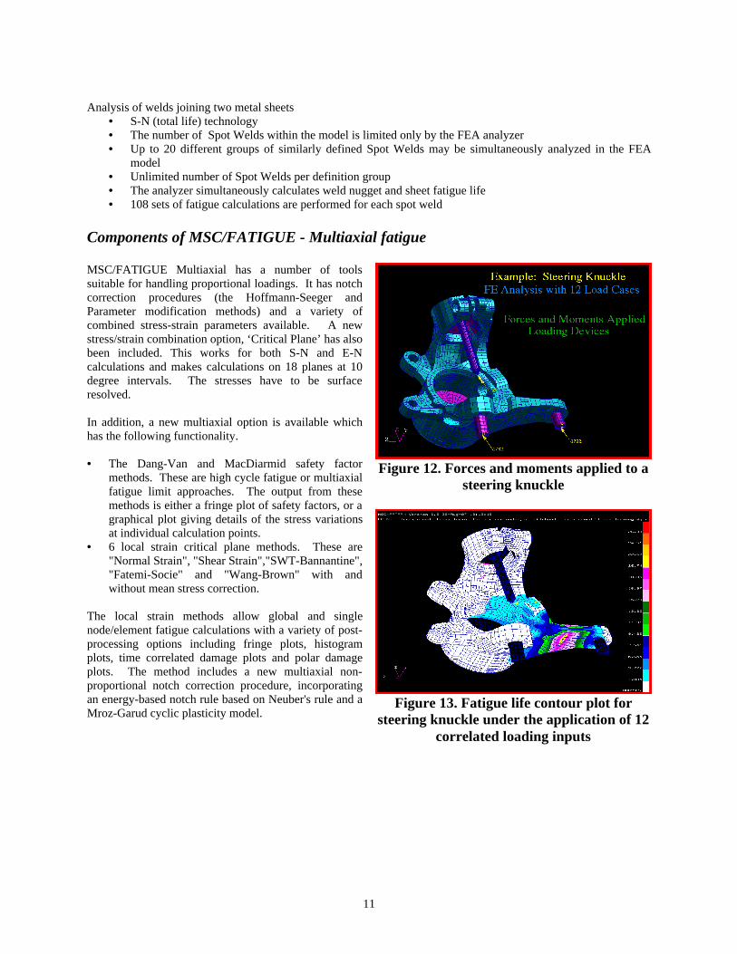
MSC/FATIGUE Multiaxial has a number of toolssuitable for handling proportional loadings. It has notchcorrection procedures (the Hoffmann-Seeger andParameter modification methods) and a variety ofcombined stress-strain parameters available. A newstress/strain combination option, ‘Critical Plane’ has alsobeen included. This works for both S-N and E-Ncalculations and makes calculations on 18 planes at 10degree intervals. The stresses have to be surfaceresolved.

In addition, a new multiaxial option is available whichhas the following functionality.

• The Dang-Van and MacDiarmid safety factormethods. These are high cycle fatigue or multiaxialfatigue limit approaches. The output from thesemethods is either a fringe plot of safety factors, or agraphical plot giving details of the stress variationsat individual calculation points.

• 6 local strain critical plane methods. These are"Normal Strain", "Shear Strain","SWT-Bannantine","Fatemi-Socie" and "Wang-Brown" with andwithout mean stress correction.

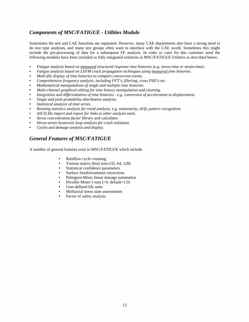
The local strain methods allow global and singlenode/element fatigue calculations with a variety of post-processing options including fringe plots, histogramplots, time correlated damage plots and polar damageplots. The method includes a new multiaxial non-proportional notch correction procedure, incorporatingan energy-based notch rule based on Neuber's rule and aMroz-Garud cyclic plasticity model.

Figure 12. Forces and moments applied to asteering knuckle

Figure 13. Fatigue life contour plot forsteering knuckle under the application of 12

correlated loading inputs

12

Components of MSC/FATIGUE - Utilities Module

Sometimes the test and CAE functions are separated. However, many CAE departments also have a strong need todo test type analyses, and many test groups often want to interface with the CAE world. Sometimes this mightinclude the pre-processing of data for a subsequent FE analysis. In order to cater for this customer need thefollowing modules have been included as fully integrated solutions in MSC/FATIGUE Utilities as described below.

• Fatigue analysis based on measured structural response time histories (e.g. stress-time or strain-time).• Fatigue analysis based on LEFM crack propagation techniques using measured time histories.• Multi-file display of time histories to compare concurrent events.• Comprehensive frequency analysis, including FFT’s, filtering, cross PSD’s etc.• Mathematical manipulations of single and multiple time histories.• Multi-channel graphical editing for time history manipulation and cleaning.• Integration and differentiation of time histories - e.g. conversion of acceleration to displacement.• Single and joint probability distribution analysis.• Statistical analysis of time series.• Running statistics analysis for trend analysis, e.g. stationarity, drift, pattern recognition.• ASCII file import and export for links to other analysis tools.• Stress concentration factor library and calculator.• Stress-strain hysteresis loop analysis for crack initiation.• Cycles and damage analysis and display.

General Features of MSC/FATIGUE

A number of general features exist in MSC/FATIGUE which include

• Rainflow cycle counting• Various matrix (bin) sizes (32, 64, 128)• Statistical confidence parameters• Surface finish/treatment corrections• Palmgren-Miner linear damage summation• Flexible Miner’s sum (>0, default=1.0)• User-defined life units• Multiaxial stress state assessments• Factor of safety analysis

13

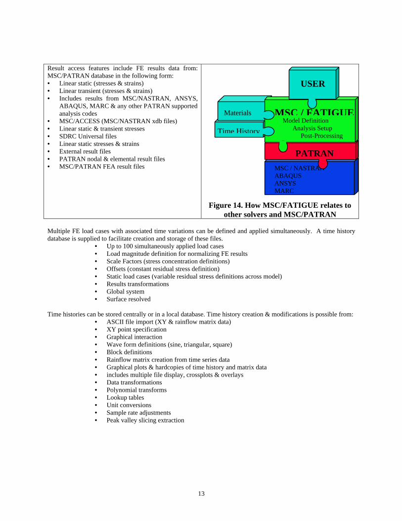
Result access features include FE results data from:MSC/PATRAN database in the following form:• Linear static (stresses & strains)• Linear transient (stresses & strains)• Includes results from MSC/NASTRAN, ANSYS,

ABAQUS, MARC & any other PATRAN supportedanalysis codes

• MSC/ACCESS (MSC/NASTRAN xdb files)• Linear static & transient stresses• SDRC Universal files• Linear static stresses & strains• External result files• PATRAN nodal & elemental result files• MSC/PATRAN FEA result files

Figure 14. How MSC/FATIGUE relates toother solvers and MSC/PATRAN

Multiple FE load cases with associated time variations can be defined and applied simultaneously. A time historydatabase is supplied to facilitate creation and storage of these files.

• Up to 100 simultaneously applied load cases• Load magnitude definition for normalizing FE results• Scale Factors (stress concentration definitions)• Offsets (constant residual stress definition)• Static load cases (variable residual stress definitions across model)• Results transformations• Global system• Surface resolved

Time histories can be stored centrally or in a local database. Time history creation & modifications is possible from:• ASCII file import (XY & rainflow matrix data)• XY point specification• Graphical interaction• Wave form definitions (sine, triangular, square)• Block definitions• Rainflow matrix creation from time series data• Graphical plots & hardcopies of time history and matrix data• includes multiple file display, crossplots & overlays• Data transformations• Polynomial transforms• Lookup tables• Unit conversions• Sample rate adjustments• Peak valley slicing extraction

Time History

Materials

MSC / NASTRANABAQUSANSYSMARC

PATRAN

MSC / FATIGUEModel Definition Analysis Setup Post-Processing

USER

14

A materials database manager stores and manipulates a library of cyclic material properties. Features include:• Approximately 200 materials (steels) supplied• Add, create or modify your own or supplied materials data (Imperial & SI units supported)• Generate materials data from UTS & E• Weld classifier based on BS7608• Graphical display of:• Component & material S-N curves• Cyclic & monotonic stress/strain curves• Strain-life curves• Elastic-plastic lines• Fatigue limits (endurance limits)• Graphical display, hardcopies & tabular comparison of materials

Figure 15. The 3 alternative material curves used in fatigue analysis

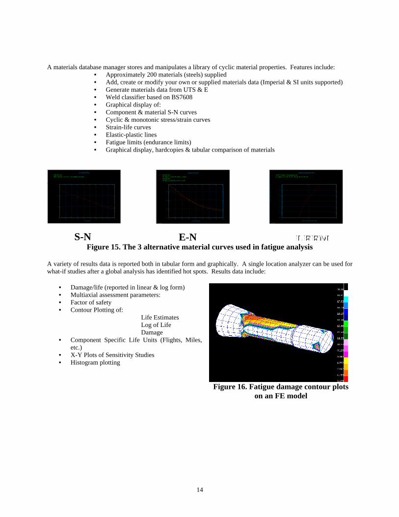
A variety of results data is reported both in tabular form and graphically. A single location analyzer can be used forwhat-if studies after a global analysis has identified hot spots. Results data include:

• Damage/life (reported in linear & log form)• Multiaxial assessment parameters:• Factor of safety• Contour Plotting of:

Life EstimatesLog of LifeDamage

• Component Specific Life Units (Flights, Miles,etc.)

• X-Y Plots of Sensitivity Studies• Histogram plotting

Figure 16. Fatigue damage contour plotson an FE model

S-N E-N_ LEFMLEFM

S-N Data Plot

MANTEN_SNSRI1: 3162 b1: -0.2 b2: 0 E: 2.034E5 UTS: 600

1E1

1E2

1E3

1E4

S

R

MP

1E0 1E1 1E2 1E3 1E4 1E5 1E6 1E7 1E8 1E9

Life (Cycles)

nCode nSoft

Strain Life PlotBS4360-50DSf': 1036 b: -0.123 Ef': 0.622 c: -0.618

BS4360-43CSf': 930 b: -0.103 Ef': 0.173 c: -0.437

1E-4

1E-3

1E-2

1E-1

1E0 1E1 1E2 1E3 1E4 1E5 1E6 1E7 1E8

Life (Reversals)

nCode nSoft

Delta K Apparent Plot2024-T3: Ratio 0 Environment: AIRC: 1.86E-11 m: 4.05 Kc: 31 D0: 3.6 D1: 0.7 Rc: 0.8

1E-11

1E-10

1E-9

1E-8

1E-7

1E-6

da/dN (m/cycle)

1E0 1E1 1E2

Delta K Apparent (MPa m1/2)

15

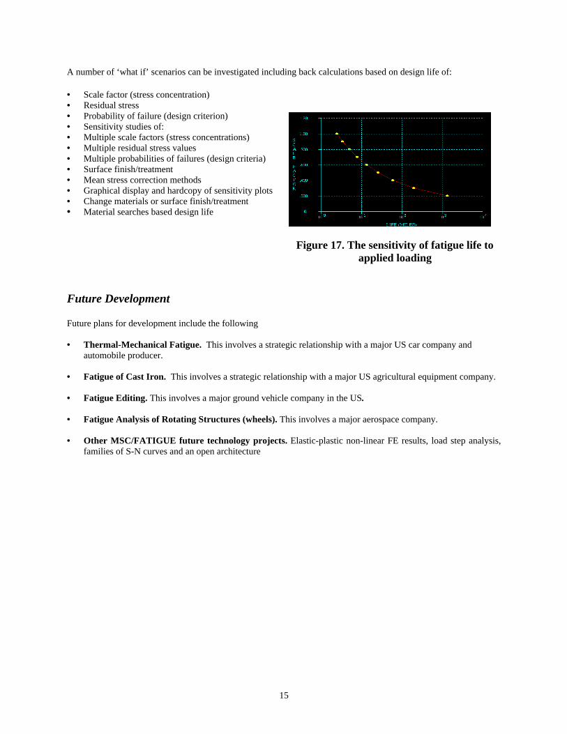
A number of ‘what if’ scenarios can be investigated including back calculations based on design life of:

• Scale factor (stress concentration)• Residual stress• Probability of failure (design criterion)• Sensitivity studies of:• Multiple scale factors (stress concentrations)• Multiple residual stress values• Multiple probabilities of failures (design criteria)• Surface finish/treatment• Mean stress correction methods• Graphical display and hardcopy of sensitivity plots• Change materials or surface finish/treatment• Material searches based design life

Figure 17. The sensitivity of fatigue life toapplied loading

Future Development

Future plans for development include the following

• Thermal-Mechanical Fatigue. This involves a strategic relationship with a major US car company andautomobile producer.

• Fatigue of Cast Iron. This involves a strategic relationship with a major US agricultural equipment company.

• Fatigue Editing. This involves a major ground vehicle company in the US.

• Fatigue Analysis of Rotating Structures (wheels). This involves a major aerospace company.

• Other MSC/FATIGUE future technology projects. Elastic-plastic non-linear FE results, load step analysis,families of S-N curves and an open architecture