Embed Size (px)
Citation preview
FIRE-FIGHTING-MANIPULATOR
Number Contents
1 Parameters of manipulator
2 Workspace of manipulator
3 Forward kinematics of manipulator
4 Inverse kinematics of manipulator
5 Dynamics of manipulator
6 Control of manipulator by using PD control
7 Control of manipulator by using Sliding mode control
8 Compare between result’s PD control and result’s Sliding mode control
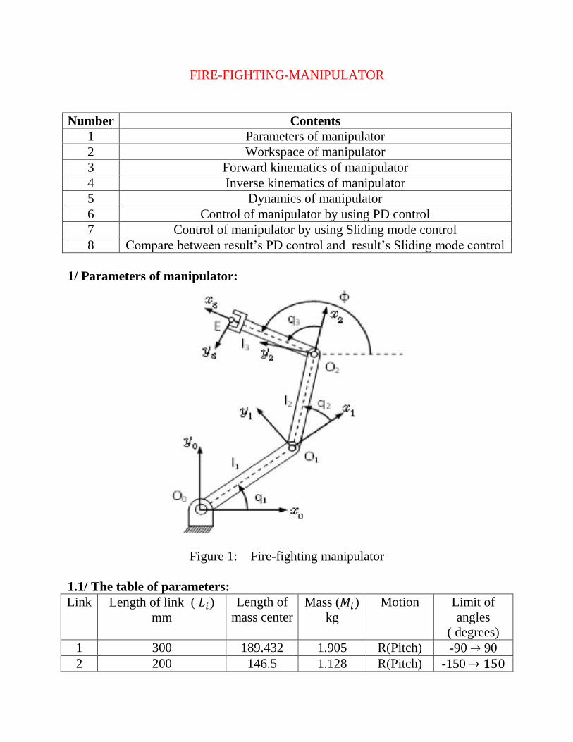
1/ Parameters of manipulator:
Figure 1: Fire-fighting manipulator
1.1/ The table of parameters:
Link
Length of link (
mm
Length of
mass center Mass (
kg
Motion Limit of
angles
( degrees)
1 300 189.432 1.905 R(Pitch) -90 90
2 200 146.5 1.128 R(Pitch) -150
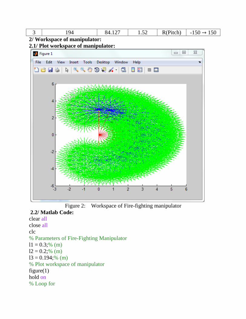
3 194 84.127 1.52 R(Pitch) -150 150
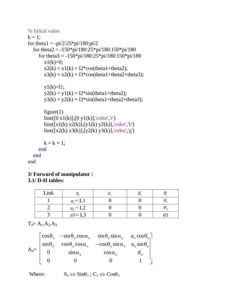
2/ Workspace of manipulator:
2.1/ Plot workspace of manipulator:
Figure 2: Workspace of Fire-fighting manipulator
2.2/ Matlab Code:
clear all
close all
clc
% Parameters of Fire-Fighting Manipulator
l1 = 0.3;% (m)
l2 = 0.2;% (m)
l3 = 0.194;% (m)
% Plot workspace of manipulator
figure(1)
hold on
% Loop for
% Initial value
k = 1;
for theta1 = -pi/2:25*pi/180:pi/2
for theta2 = -150*pi/180:25*pi/180:150*pi/180
for theta3 = -150*pi/180:25*pi/180:150*pi/180
x1(k)=0;
x2(k) = x1(k) + l2*cos(theta1+theta2);
x3(k) = x2(k) + l3*cos(theta1+theta2+theta3);
y1(k)=l1;
y2(k) = y1(k) + l2*sin(theta1+theta2);
y3(k) = y2(k) + l3*sin(theta1+theta2+theta3);
figure(1)
line([0 x1(k)],[0 y1(k)],'color','r')
line([x1(k) x2(k)],[y1(k) y2(k)],'color','b')
line([x2(k) x3(k)],[y2(k) y3(k)],'color','g')
k = k + 1;
end
end
end
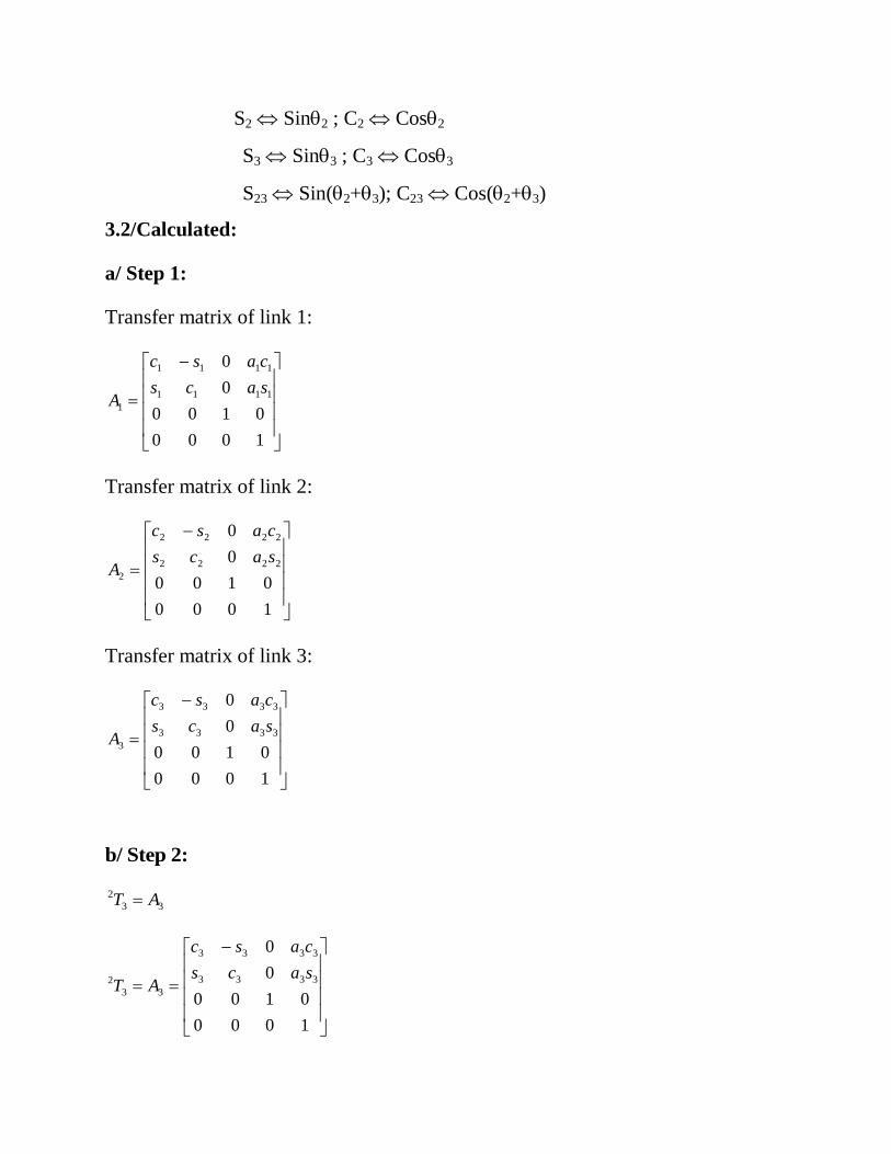
3/ Forward of manipulator :
3.1/ D-H tables:
Link ia i id i
1 1a = L1 0 0 1
2 2a = L2 0 0 2
3 3a = L3 0 0 3
T4= A1.A2.A3
An=
n n n n n n n
n n n n n n n
n n n
cos sin cos sin sin a cos
sin cos cos cos sin a sin
0 sin cos d
0 0 0 1
Where: S1 Sin1 ; C1 Cos1
S2 Sin2 ; C2 Cos2
S3 Sin3 ; C3 Cos3
S23 Sin(2+3); C23 Cos(2+3)
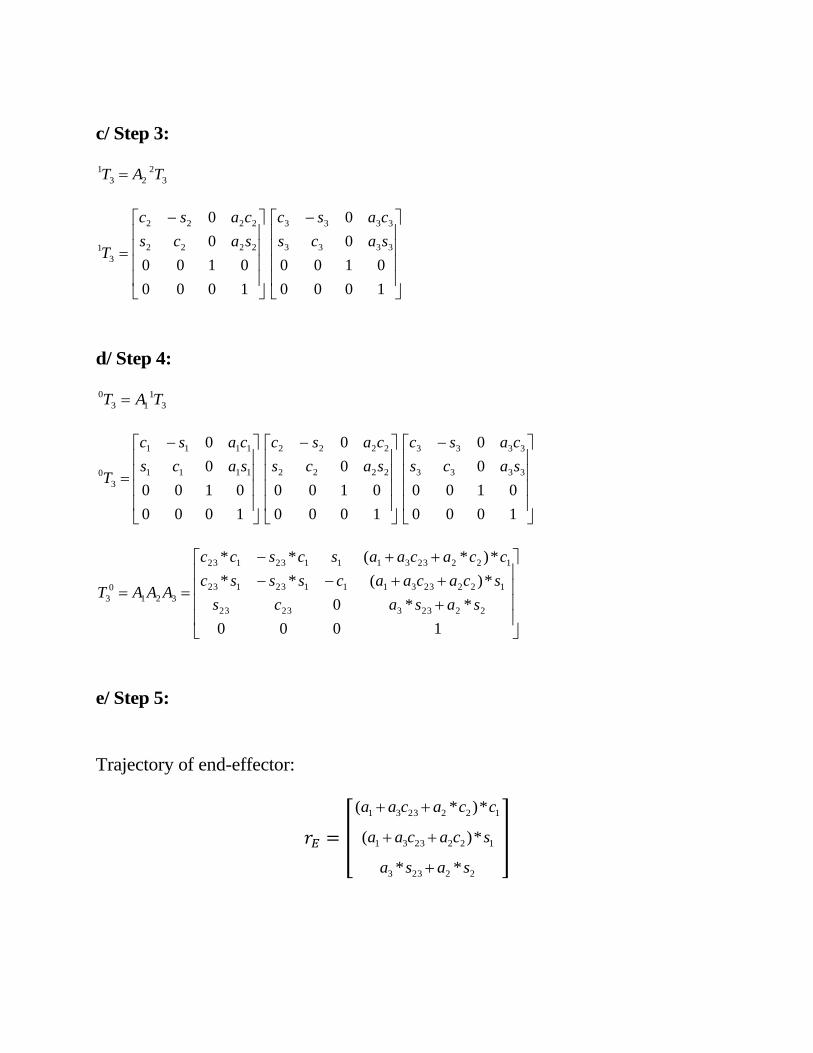
3.2/Calculated:
a/ Step 1:
Transfer matrix of link 1:
1000
0100
0
0
1111
1111
1
sacs
casc
A
Transfer matrix of link 2:
1000
0100
0
0
2222
2222
2
sacs
casc
A
Transfer matrix of link 3:
1000
0100
0
0
3333
3333
3
sacs
casc
A
b/ Step 2:
33
2 AT
1000
0100
0
0
3333
3333
33
2sacs
casc
AT
c/ Step 3:
3
2
23
1 TAT
1000
0100
0
0
2222
2222
3
1sacs
casc
T
1000
0100
0
0
3333
3333
sacs
casc
d/ Step 4:
3
1
13
0 TAT
1000
0100
0
0
1111
1111
3
0sacs
casc
T
1000
0100
0
0
2222
2222
sacs
casc
1000
0100
0
0
3333
3333
sacs
casc
1000
**0
*)(**
*)*(**
222332323
12223311123123
12223311123123
321
0
3sasacs
scacaacsssc
ccacaascscc
AAAT
e/ Step 5:
Trajectory of end-effector:
[
1222331 *)*( ccacaa
1222331 *)( scacaa
22233 ** sasa
]
x x x x
y y y y
E 4
z z z z
n o a p
n o a pT T
n o a p
0 0 0 1
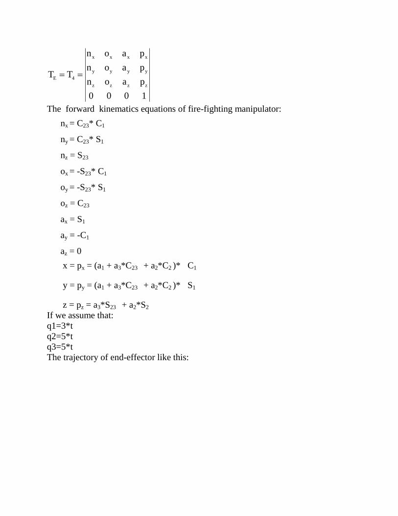
The forward kinematics equations of fire-fighting manipulator:
nx = C23* C1
ny = C23* S1
nz = S23
ox = -S23* C1
oy = -S23* S1
oz = C23
ax = S1
ay = -C1
az = 0
x = px = (a1 + a3*C23 + a2*C2 )* C1
y = py = (a1 + a3*C23 + a2*C2 )* S1
z = pz = a3*S23 + a2*S2
If we assume that:
q1=3*t
q2=5*t
q3=5*t
The trajectory of end-effector like this:
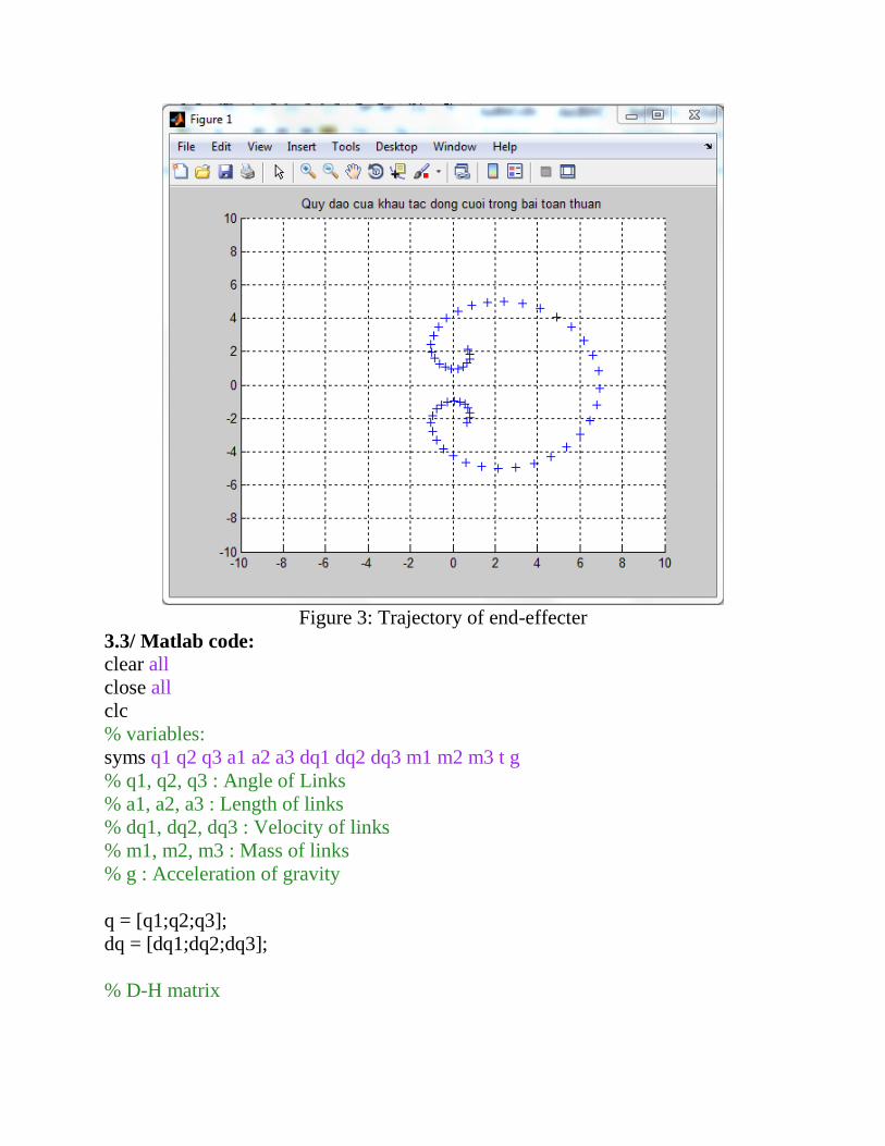
Figure 3: Trajectory of end-effecter
3.3/ Matlab code:
clear all
close all
clc
% variables:
syms q1 q2 q3 a1 a2 a3 dq1 dq2 dq3 m1 m2 m3 t g
% q1, q2, q3 : Angle of Links
% a1, a2, a3 : Length of links
% dq1, dq2, dq3 : Velocity of links
% m1, m2, m3 : Mass of links
% g : Acceleration of gravity
q = [q1;q2;q3];
dq = [dq1;dq2;dq3];
% D-H matrix
A_01=[ cos(q1) -sin(q1) 0 a1*cos(q1); sin(q1) cos(q1) 0 a1*sin(q1); 0 0 1 0;0 0 0
1];
A_12=[ cos(q2) -sin(q2) 0 a2*cos(q2); sin(q2) cos(q2) 0 a2*sin(q2); 0 0 1 0;0 0 0
1];
A_23=[ cos(q3) -sin(q3) 0 a3*cos(q3); sin(q3) cos(q3) 0 a3*sin(q3); 0 0 1 0;0 0 0
1];
R_01=A_01(1:3,1:3);
A_02=simplify(A_01*A_12);
R_02=A_02(1:3,1:3);
A_03=A_01*A_12*A_23;
A_03 = simplify(A_03);
R_03 = A_03(1:3,1:3);
% End-effector
rE = A_03(1:3,4);
rA = A_02(1:3,4);
rB = A_01(1:3,4);
v_qE = simplify(jacobian(rE,q)*dq);
R_0E = A_03(1:3,1:3);
diff_R_0E = diff(R_0E,q1)*dq1+diff(R_0E,q2)*dq2+diff(R_0E,q3)*dq3;
% Velocity
omega_curve = diff_R_0E*R_0E.';
omega_curve = simplify(omega_curve);
omega = [omega_curve(3,2) omega_curve(1,3) omega_curve(2,1)];
sub_rE = simplify(subs(rE,{q1 q2 q3 a1 a2 a3},{3*t 5*t 5*t 3 2 1.94}));
% Calculated and figure
time=-pi/6:0.02:pi/6;
num_rE=zeros(3,length(time));
for j=1:length(time)
num_rE(:,j) = subs(sub_rE,t,time(j));
end
figure(1)
clf
title('Trajectory of end-effector')
hold on
grid on
axis([-10, 10, -10, 10 ,-5, 5])
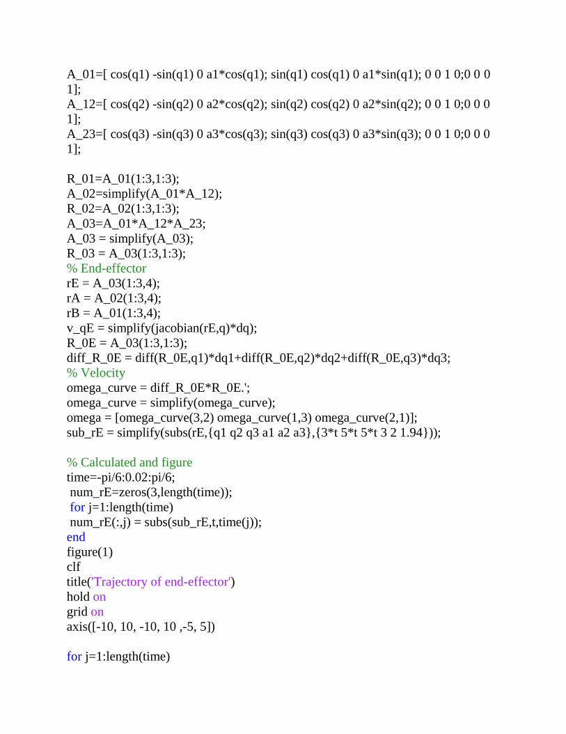
for j=1:length(time)
plot3(num_rE(1,j),num_rE(2,j),num_rE(3,j),'b+');
plot(rob,[3*time(j),5*time(j),5*time(j)]);
pause(1/30);
end
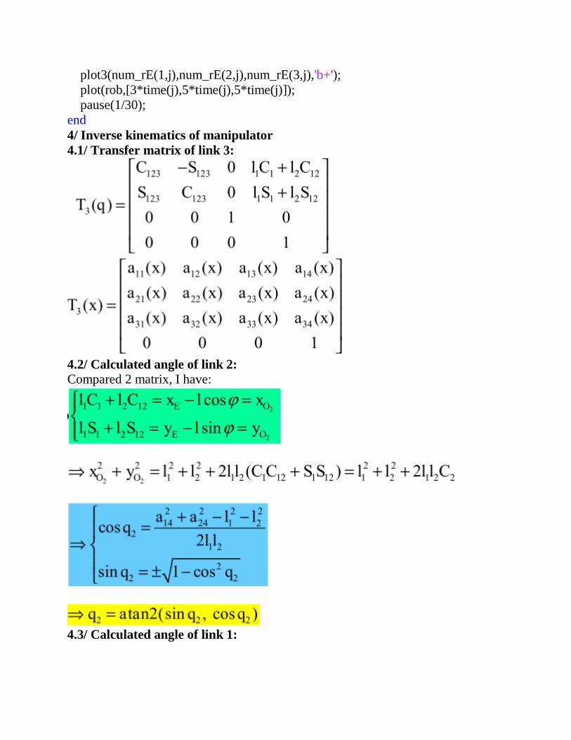
4/ Inverse kinematics of manipulator
4.1/ Transfer matrix of link 3:
4.2/ Calculated angle of link 2:
Compared 2 matrix, I have:
4.3/ Calculated angle of link 1:
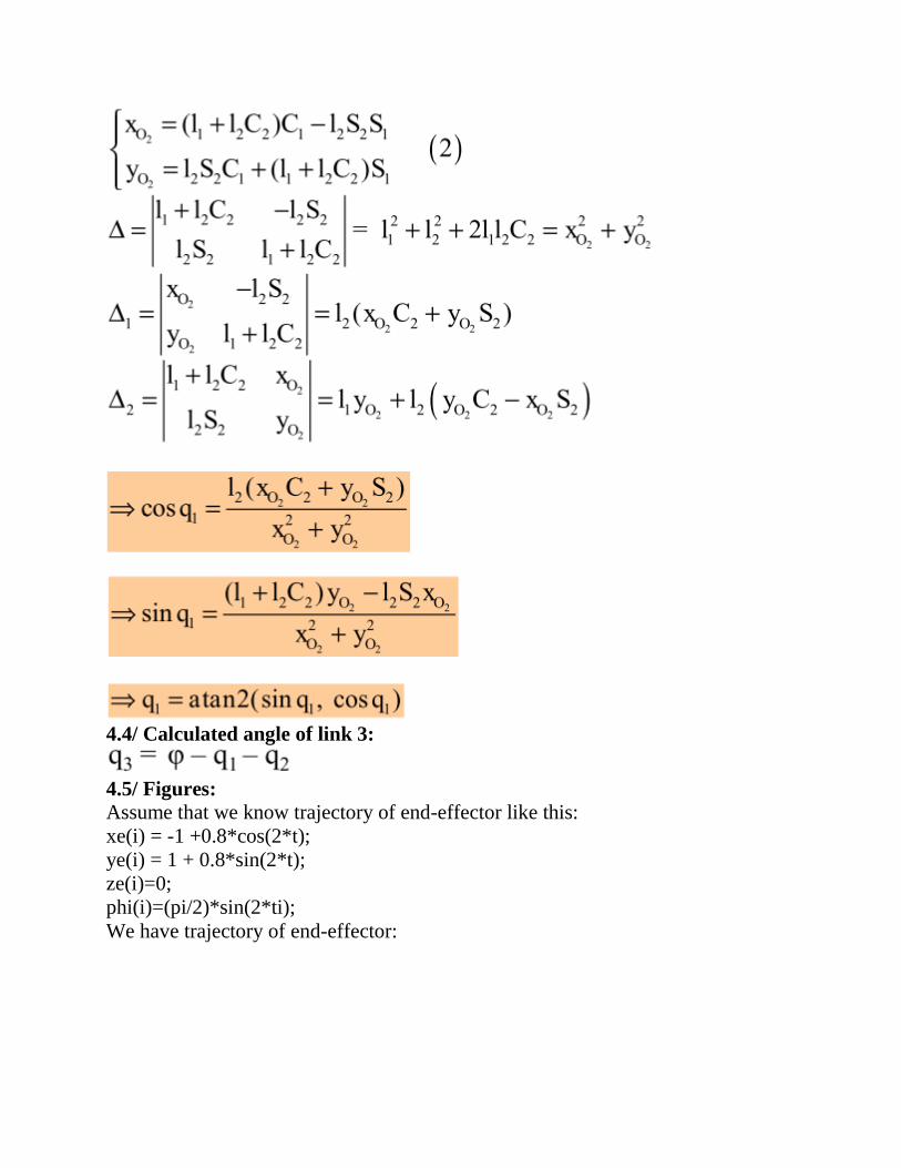
4.4/ Calculated angle of link 3:
4.5/ Figures:
Assume that we know trajectory of end-effector like this:
xe(i) = -1 +0.8*cos(2*t);
ye(i) = 1 + 0.8*sin(2*t);
ze(i)=0;
phi(i)=(pi/2)*sin(2*ti);
We have trajectory of end-effector:
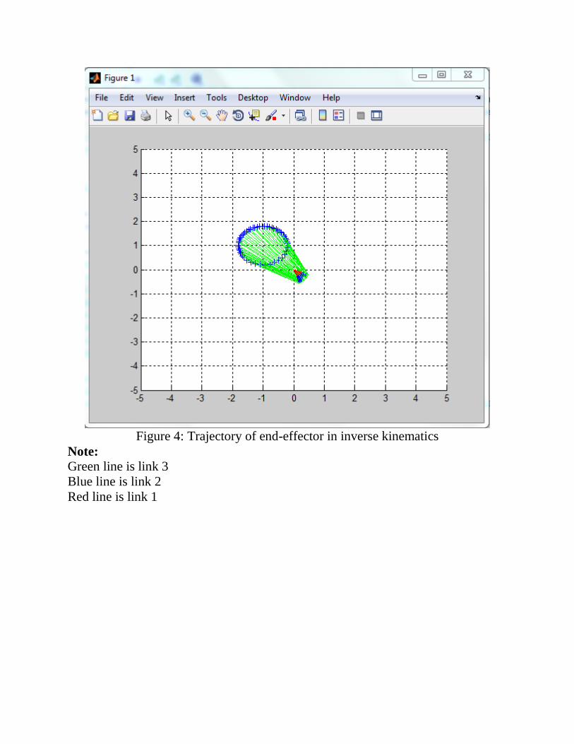
Figure 4: Trajectory of end-effector in inverse kinematics
Note:
Green line is link 3
Blue line is link 2
Red line is link 1
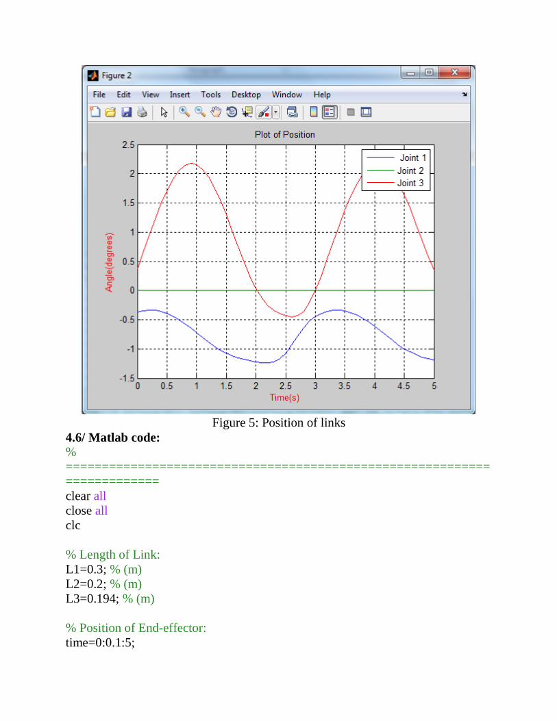
Figure 5: Position of links
4.6/ Matlab code:
%
===========================================================
=============
clear all
close all
clc
% Length of Link:
L1=0.3; % (m)
L2=0.2; % (m)
L3=0.194; % (m)
% Position of End-effector:
time=0:0.1:5;
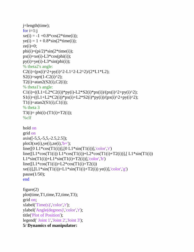
j=length(time);
for i=1:j
xe(i) = -1 +0.8*cos(2*time(i));
ye(i) = 1 + 0.8*sin(2*time(i));
ze(i)=0;
phi(i)=(pi/2)*sin(2*time(i));
px(i)=xe(i)-L3*cos(phi(i));
py(i)=ye(i)-L3*sin(phi(i));
% theta2's angle:
C2(i)=(px(i)^2+py(i)^2-L1^2-L2^2)/(2*L1*L2);
S2(i)=sqrt(1-C2(i)^2);
T2(i)=atan2(S2(i),C2(i));
% theta1's angle:
C1(i)=((L1+L2*C2(i))*py(i)-L2*S2(i)*px(i))/(px(i)^2+py(i)^2);
S1(i)=((L1+L2*C2(i))*px(i)+L2*S2(i)*py(i))/(px(i)^2+py(i)^2);
T1(i)=atan2(S1(i),C1(i));
% theta 3
T3(i)= phi(i)-(T1(i)+T2(i));
%clf
hold on
grid on
axis([-5,5,-5,5,-2.5,2.5]);
plot3(xe(i),ye(i),ze(i),'b+');
line([0 L1*cos(T1(i))],[0 L1*sin(T1(i))],'color','r')
line([L1*cos(T1(i)) L1*cos(T1(i))+L2*cos(T1(i)+T2(i))],[ L1*sin(T1(i))
L1*sin(T1(i))+L1*sin(T1(i)+T2(i))],'color','b')
line([L1*cos(T1(i))+L2*cos(T1(i)+T2(i))
xe(i)],[L1*sin(T1(i))+L1*sin(T1(i)+T2(i)) ye(i)],'color','g')
pause(1/50);
end
figure(2)
plot(time,T1,time,T2,time,T3);
grid on;
xlabel('Time(s)','color','r');
ylabel('Angle(degrees)','color','r');
title('Plot of Position');
legend(' Joint 1','Joint 2','Joint 3');
5/ Dynamics of manipulator:
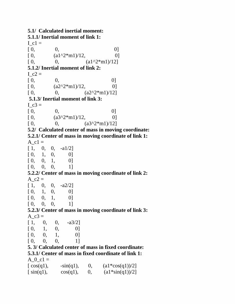
5.1/ Calculated inertial moment:
5.1.1/ Inertial moment of link 1:
I_c1 =
[ 0, 0, 0]
[ 0, (a1^2*m1)/12, 0]
[ 0, 0, (a1^2*m1)/12]
5.1.2/ Inertial moment of link 2:
I_c2 =
[ 0, 0, 0]
[ 0, (a2^2*m1)/12, 0]
[ 0, 0, (a2^2*m1)/12]
5.1.3/ Inertial moment of link 3:
I_c3 =
[ 0, 0, 0]
[ 0, (a3^2*m1)/12, 0]
[ 0, 0, (a3^2*m1)/12]
5.2/ Calculated center of mass in moving coordinate:
5.2.1/ Center of mass in moving coordinate of link 1:
A_c1 =
[ 1, 0, 0, -a1/2]
[ 0, 1, 0, 0]
[ 0, 0, 1, 0]
[ 0, 0, 0, 1]
5.2.2/ Center of mass in moving coordinate of link 2:
A_c2 =
[ 1, 0, 0, -a2/2]
[ 0, 1, 0, 0]
[ 0, 0, 1, 0]
[ 0, 0, 0, 1]
5.2.3/ Center of mass in moving coordinate of link 3:
A_c3 =
[ 1, 0, 0, -a3/2]
[ 0, 1, 0, 0]
[ 0, 0, 1, 0]
[ 0, 0, 0, 1]
5. 3/ Calculated center of mass in fixed coordinate:
5.3.1/ Center of mass in fixed coordinate of link 1:
A_0_c1 =
[ cos(q1), -sin(q1), 0, (a1*cos(q1))/2]
[ sin(q1), cos(q1), 0, (a1*sin(q1))/2]
[ 0, 0, 1, 0]
[ 0, 0, 0, 1]
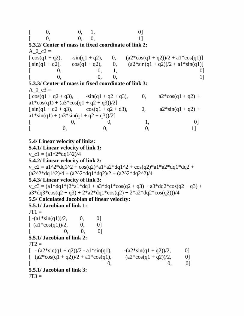
5.3.2/ Center of mass in fixed coordinate of link 2:
A_0_c2 =
[ cos(q1 + q2), -sin(q1 + q2), 0, (a2*cos(q1 + q2))/2 + a1*cos(q1)]
[ sin(q1 + q2), cos(q1 + q2), 0, (a2*sin(q1 + q2))/2 + a1*sin(q1)]
[ 0, 0, 1, 0]
[ 0, 0, 0, 1]
5.3.3/ Center of mass in fixed coordinate of link 3:
A_0_c3 =
[ cos(q1 + q2 + q3), -sin(q1 + q2 + q3), 0, a2*cos(q1 + q2) +
a1*cos(q1) + (a3*cos(q1 + q2 + q3))/2]
[ sin(q1 + q2 + q3), cos(q1 + q2 + q3), 0, a2*sin(q1 + q2) +
a1*sin(q1) + (a3*sin(q1 + q2 + q3))/2]
[ 0, 0, 1, 0]
[ 0, 0, 0, 1]
5.4/ Linear velocity of links:
5.4.1/ Linear velocity of link 1:
v_c1 = (a1^2*dq1^2)/4
5.4.2/ Linear velocity of link 2:
v_c2 = a1^2*dq1^2 + cos(q2)*a1*a2*dq1^2 + cos(q2)*a1*a2*dq1*dq2 +
(a2^2*dq1^2)/4 + (a2^2*dq1*dq2)/2 + (a2^2*dq2^2)/4
5.4.3/ Linear velocity of link 3:
v_c3 = (a1*dq1*(2*a1*dq1 + a3*dq1*cos(q2 + q3) + a3*dq2*cos(q2 + q3) +
a3*dq3*cos(q2 + q3) + 2*a2*dq1*cos(q2) + 2*a2*dq2*cos(q2)))/4
5.5/ Calculated Jacobian of linear velocity:
5.5.1/ Jacobian of link 1:
JT1 =
[ -(a1*sin(q1))/2, 0, 0]
[ (a1*cos(q1))/2, 0, 0]
[ 0, 0, 0]
5.5.1/ Jacobian of link 2:
JT2 =
[ - (a2*sin(q1 + q2))/2 - a1*sin(q1), -(a2*sin(q1 + q2))/2, 0]
[ (a2*cos(q1 + q2))/2 + a1*cos(q1), (a2*cos(q1 + q2))/2, 0]
[ 0, 0, 0]
5.5.1/ Jacobian of link 3:
JT3 =
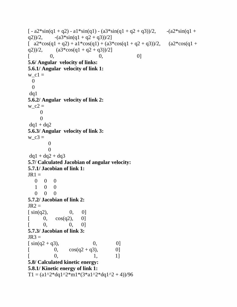
[ - a2*sin(q1 + q2) - a1*sin(q1) - (a3*sin(q1 + q2 + q3))/2, -(a2*sin(q1 +
q2))/2, -(a3*sin(q1 + q2 + q3))/2]
[ a2*cos(q1 + q2) + a1*cos(q1) + (a3*cos(q1 + q2 + q3))/2, (a2*cos(q1 +
q2))/2, (a3*cos(q1 + q2 + q3))/2]
[ 0, 0, 0]
5.6/ Angular velocity of links:
5.6.1/ Angular velocity of link 1:
w_c1 =
0
0
dq1
5.6.2/ Angular velocity of link 2: w_c2 =
0
0
dq1 + dq2
5.6.3/ Angular velocity of link 3:
w_c3 =
0
0
dq1 + dq2 + dq3
5.7/ Calculated Jacobian of angular velocity:
5.7.1/ Jacobian of link 1:
JR1 =
0 0 0
1 0 0
0 0 0
5.7.2/ Jacobian of link 2:
JR2 =
[ sin(q2), 0, 0]
[ 0, cos(q2), 0]
[ 0, 0, 0]
5.7.3/ Jacobian of link 3:
JR3 =
[ sin(q2 + q3), 0, 0]
[ 0, cos(q2 + q3), 0]
[ 0, 1, 1]
5.8/ Calculated kinetic energy:
5.8.1/ Kinetic energy of link 1:
T1 = (a1^2*dq1^2*m1*(3*a1^2*dq1^2 + 4))/96
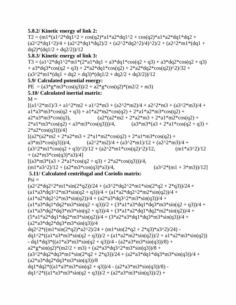
5.8.2/ Kinetic energy of link 2:
T2 = (m1*(a1^2*dq1^2 + cos(q2)*a1*a2*dq1^2 + cos(q2)*a1*a2*dq1*dq2 +
(a2^2*dq1^2)/4 + (a2^2*dq1*dq2)/2 + (a2^2*dq2^2)/4)^2)/2 + (a2^2*m1*(dq1 +
dq2)*(dq1/2 + dq2/2))/12
5.8.3/ Kinetic energy of link 3:
T3 = (a1^2*dq1^2*m1*(2*a1*dq1 + a3*dq1*cos(q2 + q3) + a3*dq2*cos(q2 + q3)
+ a3*dq3*cos(q2 + q3) + 2*a2*dq1*cos(q2) + 2*a2*dq2*cos(q2))^2)/32 +
(a3^2*m1*(dq1 + dq2 + dq3)*(dq1/2 + dq2/2 + dq3/2))/12
5.9/ Calculated potential energy:
PE = (a3*g*m3*cos(q3))/2 + a2*g*cos(q2)*(m2/2 + m3)
5.10/ Calculated inertial matrix:
M =
[(a1^2*m1)/3 + a1^2*m2 + a1^2*m3 + (a2^2*m2)/4 + a2^2*m3 + (a3^2*m3)/4 +
a1*a3*m3*cos(q2 + q3) + a1*a2*m2*cos(q2) + 2*a1*a2*m3*cos(q2) +
a2*a3*m3*cos(q3), (a2*(a2*m2 + 2*a2*m3 + 2*a1*m2*cos(q2) +
2*a1*m3*cos(q2) + a3*m3*cos(q3)))/4, (a3*m3*(a3 + 2*a1*cos(q2 + q3) +
2*a2*cos(q3)))/4]
[(a2*(a2*m2 + 2*a2*m3 + 2*a1*m2*cos(q2) + 2*a1*m3*cos(q2) +
a3*m3*cos(q3)))/4, (a2^2*m2)/4 + (a3^2*m1)/12 + (a2^2*m3)/4 +
(a3^2*m1*cos(q2 + q3)^2)/12 + (a2^2*m1*cos(q2)^2)/12, (m1*a3^2)/12
+ (a2*m3*cos(q3)*a3)/4]
[(a3*m3*(a3 + 2*a1*cos(q2 + q3) + 2*a2*cos(q3)))/4,
(m1*a3^2)/12 + (a2*m3*cos(q3)*a3)/4, (a3^2*(m1 + 3*m3))/12]
5.11/ Calculated centrifugal and Coriolis matrix:
Psi =
(a2^2*dq2^2*m1*sin(2*q2))/24 + (a3^2*dq2^2*m1*sin(2*q2 + 2*q3))/24 +
(a1*a3*dq3^2*m3*sin(q2 + q3))/4 + (a1*a2*dq2^2*m2*sin(q2))/4 +
(a1*a2*dq2^2*m3*sin(q2))/4 + (a2*a3*dq3^2*m3*sin(q3))/4 +
(a1*a3*dq1*dq2*m3*sin(q2 + q3))/2 + (3*a1*a3*dq1*dq3*m3*sin(q2 + q3))/4 +
(a1*a3*dq2*dq3*m3*sin(q2 + q3))/4 + (3*a1*a2*dq1*dq2*m2*sin(q2))/4 +
(5*a1*a2*dq1*dq2*m3*sin(q2))/4 + (3*a2*a3*dq1*dq3*m3*sin(q3))/4 +
(a2*a3*dq2*dq3*m3*sin(q3))/4
dq2^2*((m1*sin(2*q2)*a2^2)/24 + (m1*sin(2*q2 + 2*q3)*a3^2)/24) -
dq1^2*((a1*a3*m3*sin(q2 + q3))/2 + (a1*a2*m2*sin(q2))/2 + a1*a2*m3*sin(q2))
- dq1*dq3*((a1*a3*m3*sin(q2 + q3))/4 - (a2*a3*m3*sin(q3))/8) +
a2*g*sin(q2)*(m2/2 + m3) + (a2*a3*dq3^2*m3*sin(q3))/8 +
(a3^2*dq2*dq3*m1*sin(2*q2 + 2*q3))/24 + (a2*a3*dq1*dq3*m3*sin(q3))/4 +
(a2*a3*dq2*dq3*m3*sin(q3))/8
dq1*dq2*((a1*a3*m3*sin(q2 + q3))/4 - (a2*a3*m3*sin(q3))/8) -
dq1^2*((a1*a3*m3*sin(q2 + q3))/2 + (a2*a3*m3*sin(q3))/2) +
dq1*dq2*((a2*(2*a1*m2*sin(q2) + 2*a1*m3*sin(q2)))/8 - (a2*a3*m3*sin(q3))/8)
+ (a3*g*m3*sin(q3))/2 + (a2^2*dq2^2*m1*sin(2*q2))/24
5.12/Matlab Code:
clear all
close all
clc
% Variables:
syms q1 q2 q3 a1 a2 a3 dq1 dq2 dq3 m1 m2 m3 t g
q = [q1;q2;q3];
dq = [dq1;dq2;dq3];
% D-H matrix
A_01=[ cos(q1) -sin(q1) 0 a1*cos(q1); sin(q1) cos(q1) 0 a1*sin(q1); 0 0 1 0;0 0 0
1];
A_12=[ cos(q2) -sin(q2) 0 a2*cos(q2); sin(q2) cos(q2) 0 a2*sin(q2); 0 0 1 0;0 0 0
1];
A_23=[ cos(q3) -sin(q3) 0 a3*cos(q3); sin(q3) cos(q3) 0 a3*sin(q3); 0 0 1 0;0 0 0
1];
R_01=A_01(1:3,1:3);
A_03=A_01*A_12*A_23;
A_02=simplify(A_01*A_12);
R_02=A_02(1:3,1:3);
A_03 = simplify(A_03);
R_03 = A_03(1:3,1:3);
% inertial moment
I_c1 = [0 0 0;0 m1*a1^2/12 0;0 0 m1*a1^2/12]
I_c2 = [0 0 0;0 m1*a2^2/12 0;0 0 m1*a2^2/12]
I_c3 = [0 0 0;0 m1*a3^2/12 0;0 0 m1*a3^2/12]
% center of mass in moving coordinate
A_c1 = [1 0 0 -a1/2;0 1 0 0;0 0 1 0;0 0 0 1]
A_c2 = [1 0 0 -a2/2;0 1 0 0;0 0 1 0;0 0 0 1]
A_c3 = [1 0 0 -a3/2;0 1 0 0;0 0 1 0;0 0 0 1]
% transforming into fixed coordinate
A_0_c1 = A_01*A_c1
A_0_c2 = simplify(A_02*A_c2)
A_0_c3 = simplify(A_03*A_c3)
r_0_c1 = A_0_c1(1:3,4);
r_0_c2 = A_0_c2(1:3,4);
r_0_c3 = A_0_c3(1:3,4);
% Linear velocity
v_0_c1 = simplify(jacobian(r_0_c1,q)*dq);
v_0_c2 = simplify(jacobian(r_0_c2,q)*dq);
v_0_c3 = simplify(jacobian(r_0_c3,q)*dq);
v_c1 = simplify(v_0_c1.'*v_0_c1)
v_c2 = simplify(v_0_c2.'*v_0_c2)
v_c3 = simplify(v_0_c1.'*v_0_c3)
% Jacobian of linear velocity
JT1=simplify(jacobian(r_0_c1,q))
JT2=simplify(jacobian(r_0_c2,q))
JT3=simplify([diff(r_0_c3,q1),diff(r_0_c2,q2),diff(r_0_c3,q3)])
% Angular velocity
tmp = A_0_c1(1:3,1:3); C2 = A_0_c2(1:3,1:3); C3 = A_0_c3(1:3,1:3);
W_c1=tmp.'*(diff(tmp,q1)*dq1+diff(tmp,q2)*dq2+diff(tmp,q3)*dq3);
w_c1=simplify([W_c1(3,2);W_c1(1,3);W_c1(2,1)])
W_c2=C2.'*(diff(C2,q1)*dq1+diff(C2,q2)*dq2+diff(C2,q3)*dq3);
w_c2=simplify([W_c2(3,2);W_c2(1,3);W_c2(2,1)])
W_c3=C3.'*(diff(C3,q1)*dq1+diff(C3,q2)*dq2+diff(C3,q3)*dq3);
w_c3=simplify([W_c3(3,2);W_c3(1,3);W_c3(2,1)])
% Jacobian of angular velocity
JR1 = [0 0 0;1 0 0;0 0 0]
JR2 = [sin(q2) 0 0;0 cos(q2) 0;0 0 0]
JR3 =[sin(q2+q3) 0 0;0 cos(q2+q3) 0;0 1 1]
% kinetic energy
T1 = simplify(1/2*m1*v_c1.'*v_c1+1/2*w_c1.'*I_c1*w_c1)
T2 = simplify(1/2*m1*v_c2.'*v_c2+1/2*w_c2.'*I_c2*w_c2)
T3 = simplify(1/2*m1*v_c3.'*v_c3+1/2*w_c3.'*I_c3*w_c3)
% Manipulator Inertia Matrix
M =
JT1.'*m1*JT1+JT2.'*m2*JT2+JT3.'*m3*JT3+JR1.'*I_c1*JR1+JR2.'*I_c2*JR2+J
R3.'*I_c3*JR3;
M = simplify(M)
% Potential Energy (PE)
PE = (1/2*m2+m3)*a2*cos(q2)*g+1/2*m3*a3*cos(q3)*g
% Centrifugal/Coriolis matrix and Psi
tmp = sym(zeros(3));
Psi = sym(zeros(3,1));
for j=1:3
h = sym(0);
for k=1:3
for l=1:3
tmp(k,l) = 1/2*(diff(M(k,l),q(l))+diff(M(l,j),q(k))-
diff(M(k,l),q(j)))*dq(k)*dq(l);
h = h+tmp(k,l);
end
end
Psi(j) = -h-diff(PE,q(j));
end
Psi=simplify(Psi)
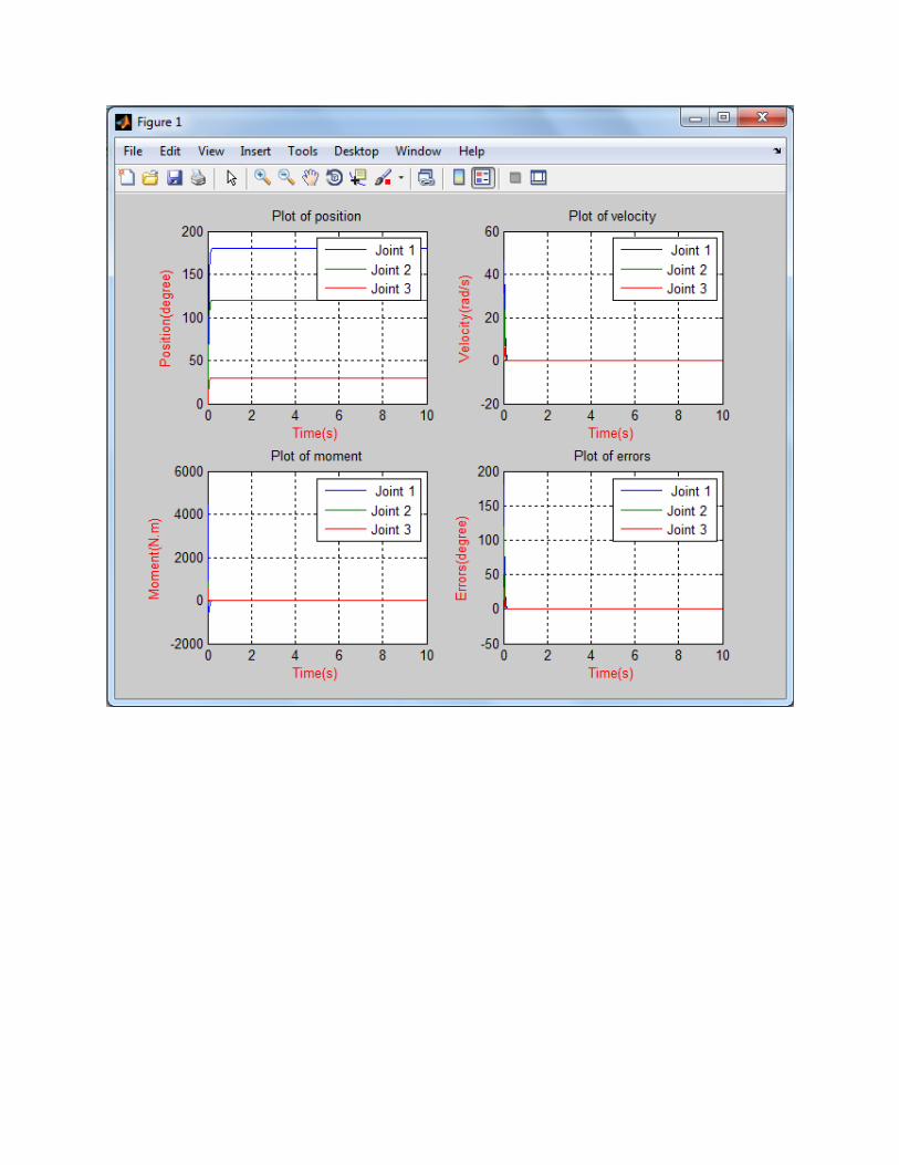
6/ Control of manipulator by using PD control :
6.1/ Using Matlab code:
function dydt=VuPD_thuong(t,x)
global kv kp m1 m2 m3 a1 a2 a3 g t1 t2 t3 ;
% Quy dao dat la sin va cos
qd(1) = 0.1*sin(pi*t);
qd(2) = 0.1*cos(pi*t);
qd(3) = 0.1*sin(pi*t + pi/6);
qdp(1) = 0.1*pi*cos(pi*t);
qdp(2) = -0.1*pi*sin(pi*t);
qdp(3) = 0.1*pi*cos(pi*t +pi/6);
qdpp(1) = -0.1*pi*pi*sin(pi*t);
qdpp(2) = -0.1*pi*pi*cos(pi*t);
qdpp(3) = -0.1*pi*pi*sin(pi*t +pi/6);
% Quy dao dat la hang so
% qd(1) = pi;
% qd(2) = 2*pi/3;
% qd(3) = pi/6;
% qdp(1) = 0;
% qdp(2) = 0;
% qdp(3) = 0;
% qdpp(1) = 0;
% qdpp(2) = 0;
% qdpp(3) = 0;
e(1) = qd(1) - x(1);
e(2) = qd(2) - x(2);
e(3) = qd(3) - x(3);
ep(1) = qdp(1) - x(4);
ep(2) = qdp(2) - x(5);
ep(3) = qdp(3) - x(6);
s1 = qdpp(1) + kv*ep(1) + kp*e(1);
s2 = qdpp(2) + kv*ep(2) + kp*e(2);
s3 = qdpp(3) + kv*ep(3) + kp*e(3);
% Matrix initial
m11= (a1^2*m1)/3 + a1^2*m2 + a1^2*m3 + (a2^2*m2)/4 + a2^2*m3 +
(a3^2*m3)/4 + a1*a3*m3*cos(x(2) + x(3)) + a1*a2*m2*cos(x(2)) +
2*a1*a2*m3*cos(x(2)) + a2*a3*m3*cos(x(3));
m12=(a2*(a2*m2 + 2*a2*m3 + 2*a1*m2*cos(x(2)) + 2*a1*m3*cos(x(2)) +
a3*m3*cos(x(3))))/4;
m13=(a3*m3*(a3 + 2*a1*cos(x(2) + x(3)) + 2*a2*cos(x(3))))/4;
m21=(a2*(a2*m2 + 2*a2*m3 + 2*a1*m2*cos(x(2)) + 2*a1*m3*cos(x(2)) +
a3*m3*cos(x(3))))/4;
m22=(a2^2*m2)/4 + (a3^2*m1)/12 + (a2^2*m3)/4 + (a3^2*m1*cos(x(2) +
x(3))^2)/12 + (a2^2*m1*cos(x(2))^2)/12;
m23=(m1*a3^2)/12 + (a2*m3*cos(x(3))*a3)/4;
m31=(a3*m3*(a3 + 2*a1*cos(x(2) + x(3)) + 2*a2*cos(x(3))))/4;
m32=(m1*a3^2)/12 + (a2*m3*cos(x(3))*a3)/4;
m33=(a3^2*(m1 + 3*m3))/12;
matM = [m11 m12 m13; m21 m22 m23; m31 m32 m33];
% Calculating Psi = Coriolis/Centrifugal + gravitational force
psi1= (a2^2*x(5)^2*m1*sin(2*x(2)))/24 + (a3^2*x(5)^2*m1*sin(2*x(2) +
2*x(3)))/24 + (a1*a3*x(6)^2*m3*sin(x(2) + x(3)))/4 +
(a1*a2*x(5)^2*m2*sin(x(2)))/4 + (a1*a2*x(5)^2*m3*sin(x(2)))/4 +
(a2*a3*x(6)^2*m3*sin(x(3)))/4 + (a1*a3*x(4)*x(5)*m3*sin(x(2) + x(3)))/2 +
(3*a1*a3*x(4)*x(6)*m3*sin(x(2) + x(3)))/4 + (a1*a3*x(5)*x(6)*m3*sin(x(2) +
x(3)))/4 + (3*a1*a2*x(4)*x(5)*m2*sin(x(2)))/4 +
(5*a1*a2*x(4)*x(5)*m3*sin(x(2)))/4 + (3*a2*a3*x(4)*x(6)*m3*sin(x(3)))/4 +
(a2*a3*x(5)*x(6)*m3*sin(x(3)))/4;
psi2=x(5)^2*((m1*sin(2*x(2))*a2^2)/24 + (m1*sin(2*x(2) + 2*x(3))*a3^2)/24) -
x(4)^2*((a1*a3*m3*sin(x(2) + x(3)))/2 + (a1*a2*m2*sin(x(2)))/2 +
a1*a2*m3*sin(x(2))) - x(4)*x(6)*((a1*a3*m3*sin(x(2) + x(3)))/4 -
(a2*a3*m3*sin(x(3)))/8) + a2*g*sin(x(2))*(m2/2 + m3) +
(a2*a3*x(6)^2*m3*sin(x(3)))/8 + (a3^2*x(5)*x(6)*m1*sin(2*x(2) + 2*x(3)))/24 +
(a2*a3*x(4)*x(6)*m3*sin(x(3)))/4 + (a2*a3*x(5)*x(6)*m3*sin(x(3)))/8;
psi3=x(4)*x(5)*((a1*a3*m3*sin(x(2) + x(3)))/4 - (a2*a3*m3*sin(x(3)))/8) -
x(4)^2*((a1*a3*m3*sin(x(2) + x(3)))/2 + (a2*a3*m3*sin(x(3)))/2) +
x(4)*x(5)*((a2*(2*a1*m2*sin(x(2)) + 2*a1*m3*sin(x(2))))/8 -
(a2*a3*m3*sin(x(3)))/8) + (a3*g*m3*sin(x(3)))/2 +
(a2^2*x(5)^2*m1*sin(2*x(2)))/24;
matPsi =[psi1; psi2; psi3];
% Control input
t1 = m11*s1 + m12*s2 + m13*s3 + psi1;
t2 = m21*s1 + m22*s2 + m23*s3 + psi2;
t3 = m31*s1 + m32*s2 + m33*s3 + psi3;
matT = [t1; t2; t3];
q2dot = inv(matM)*(matT - matPsi);
dydt = [x(4); x(5); x(6); q2dot];
global kv kp m1 m2 m3 a1 a2 a3 g t1 t2 t3 ;
m1 = 1.905;
m2 = 1.128;
m3 = 1.52;
a1 = 0.3;
a2 = 0.2;
a3 = 0.194;
g = 9.8;
wn = 40;
kv = 2*wn;
kp = wn*wn;
[t,x]=ode45(@VuPD_thuong,[0 10],[0 0 0 0 0 0]*pi/180,0.001);
% Quy dao dat la sin va cos
qd1 = 0.1*sin(pi*t);
qd2 = 0.1*cos(pi*t);
qd3 = 0.1*sin(pi*t + pi/6);
qdp1 = 0.1*pi*cos(pi*t);
qdp2 = -0.1*pi*sin(pi*t);
qdp3 = 0.1*pi*cos(pi*t +pi/6);
qdpp1 = -0.1*pi*pi*sin(pi*t);
qdpp2 = -0.1*pi*pi*cos(pi*t);
qdpp3 = -0.1*pi*pi*sin(pi*t +pi/6);
% Quy dao dat la hang so
% qd1 = pi;
% qd2 = 2*pi/3;
% qd3 = pi/6;
% qdp1 = 0;
% qdp2 = 0;
% qdp3 = 0;
% qdpp1 = 0;
% qdpp2 = 0;
% qdpp3 = 0;
e1 = qd1 - x(:,1);
e2 = qd2 - x(:,2);
e3 = qd3 - x(:,3);
ep1 = qdp1 - x(:,4);
ep2 = qdp2 - x(:,5);
ep3 = qdp3 - x(:,6);
s1 = qdpp1 + kv*ep1 + kp*e1;
s2 = qdpp2 + kv*ep2 + kp*e2;
s3 = qdpp3 + kv*ep3 + kp*e3;
% Matrix initial
m11= (a1^2*m1)/3 + a1^2*m2 + a1^2*m3 + (a2^2*m2)/4 + a2^2*m3 +
(a3^2*m3)/4 + a1*a3*m3*cos(x(2) + x(3)) + a1*a2*m2*cos(x(2)) +
2*a1*a2*m3*cos(x(2)) + a2*a3*m3*cos(x(3));
m12=(a2*(a2*m2 + 2*a2*m3 + 2*a1*m2*cos(x(2)) + 2*a1*m3*cos(x(2)) +
a3*m3*cos(x(3))))/4;
m13=(a3*m3*(a3 + 2*a1*cos(x(2) + x(3)) + 2*a2*cos(x(3))))/4;
m21=(a2*(a2*m2 + 2*a2*m3 + 2*a1*m2*cos(x(2)) + 2*a1*m3*cos(x(2)) +
a3*m3*cos(x(3))))/4;
m22=(a2^2*m2)/4 + (a3^2*m1)/12 + (a2^2*m3)/4 + (a3^2*m1*cos(x(2) +
x(3))^2)/12 + (a2^2*m1*cos(x(2))^2)/12;
m23=(m1*a3^2)/12 + (a2*m3*cos(x(3))*a3)/4;
m31=(a3*m3*(a3 + 2*a1*cos(x(2) + x(3)) + 2*a2*cos(x(3))))/4;
m32=(m1*a3^2)/12 + (a2*m3*cos(x(3))*a3)/4;
m33=(a3^2*(m1 + 3*m3))/12;
% Calculating Psi = Coriolis/Centrifugal + gravitational force
psi1= (a2^2*x(5)^2*m1*sin(2*x(2)))/24 + (a3^2*x(5)^2*m1*sin(2*x(2) +
2*x(3)))/24 + (a1*a3*x(6)^2*m3*sin(x(2) + x(3)))/4 +
(a1*a2*x(5)^2*m2*sin(x(2)))/4 + (a1*a2*x(5)^2*m3*sin(x(2)))/4 +
(a2*a3*x(6)^2*m3*sin(x(3)))/4 + (a1*a3*x(4)*x(5)*m3*sin(x(2) + x(3)))/2 +
(3*a1*a3*x(4)*x(6)*m3*sin(x(2) + x(3)))/4 + (a1*a3*x(5)*x(6)*m3*sin(x(2) +
x(3)))/4 + (3*a1*a2*x(4)*x(5)*m2*sin(x(2)))/4 +
(5*a1*a2*x(4)*x(5)*m3*sin(x(2)))/4 + (3*a2*a3*x(4)*x(6)*m3*sin(x(3)))/4 +
(a2*a3*x(5)*x(6)*m3*sin(x(3)))/4;
psi2=x(5)^2*((m1*sin(2*x(2))*a2^2)/24 + (m1*sin(2*x(2) + 2*x(3))*a3^2)/24) -
x(4)^2*((a1*a3*m3*sin(x(2) + x(3)))/2 + (a1*a2*m2*sin(x(2)))/2 +
a1*a2*m3*sin(x(2))) - x(4)*x(6)*((a1*a3*m3*sin(x(2) + x(3)))/4 -
(a2*a3*m3*sin(x(3)))/8) + a2*g*sin(x(2))*(m2/2 + m3) +
(a2*a3*x(6)^2*m3*sin(x(3)))/8 + (a3^2*x(5)*x(6)*m1*sin(2*x(2) + 2*x(3)))/24 +
(a2*a3*x(4)*x(6)*m3*sin(x(3)))/4 + (a2*a3*x(5)*x(6)*m3*sin(x(3)))/8;
psi3=x(4)*x(5)*((a1*a3*m3*sin(x(2) + x(3)))/4 - (a2*a3*m3*sin(x(3)))/8) -
x(4)^2*((a1*a3*m3*sin(x(2) + x(3)))/2 + (a2*a3*m3*sin(x(3)))/2) +
x(4)*x(5)*((a2*(2*a1*m2*sin(x(2)) + 2*a1*m3*sin(x(2))))/8 -
(a2*a3*m3*sin(x(3)))/8) + (a3*g*m3*sin(x(3)))/2 +
(a2^2*x(5)^2*m1*sin(2*x(2)))/24;
% Control input
t1 = m11*s1 + m12*s2 + m13*s3 + psi1;
t2 = m21*s1 + m22*s2 + m23*s3 + psi2;
t3 = m31*s1 + m32*s2 + m33*s3 + psi3;
figure(1)
subplot(2,2,1);
plot(t,x(:,1)*180/pi,t,x(:,2)*180/pi,t,x(:,3)*180/pi);
grid on;
xlabel('Time(s)','color','r');
ylabel('Position(degree)','color','r');
title('Plot of position');
legend(' Joint 1','Joint 2','Joint 3');
subplot(2,2,2);
plot(t,x(:,4),t,x(:,5),t,x(:,6));
grid on;
xlabel('Time(s)','color','r');
ylabel('Velocity(rad/s)','color','r');
title('Plot of velocity');
legend(' Joint 1','Joint 2','Joint 3');
subplot(2,2,3);
plot(t,t1,t,t2,t,t3);
grid on;
xlabel('Time(s)','color','r');
ylabel('Moment(N.m)','color','r');
title('Plot of moment');
legend(' Joint 1','Joint 2','Joint 3');
subplot(2,2,4);
plot(t,e1*180/pi,t,e2*180/pi,t,e3*180/pi);
grid on;
xlabel('Time(s)','color','r');
ylabel('Errors(degree)','color','r');
title('Plot of errors');
legend(' Joint 1','Joint 2','Joint 3');
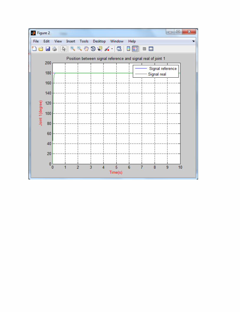
figure(2)
plot(t,qd1*180/pi,t,x(:,1)*180/pi);
grid on;
xlabel('Time(s)','color','r');
ylabel(' Joint 1(degree)','color','r');
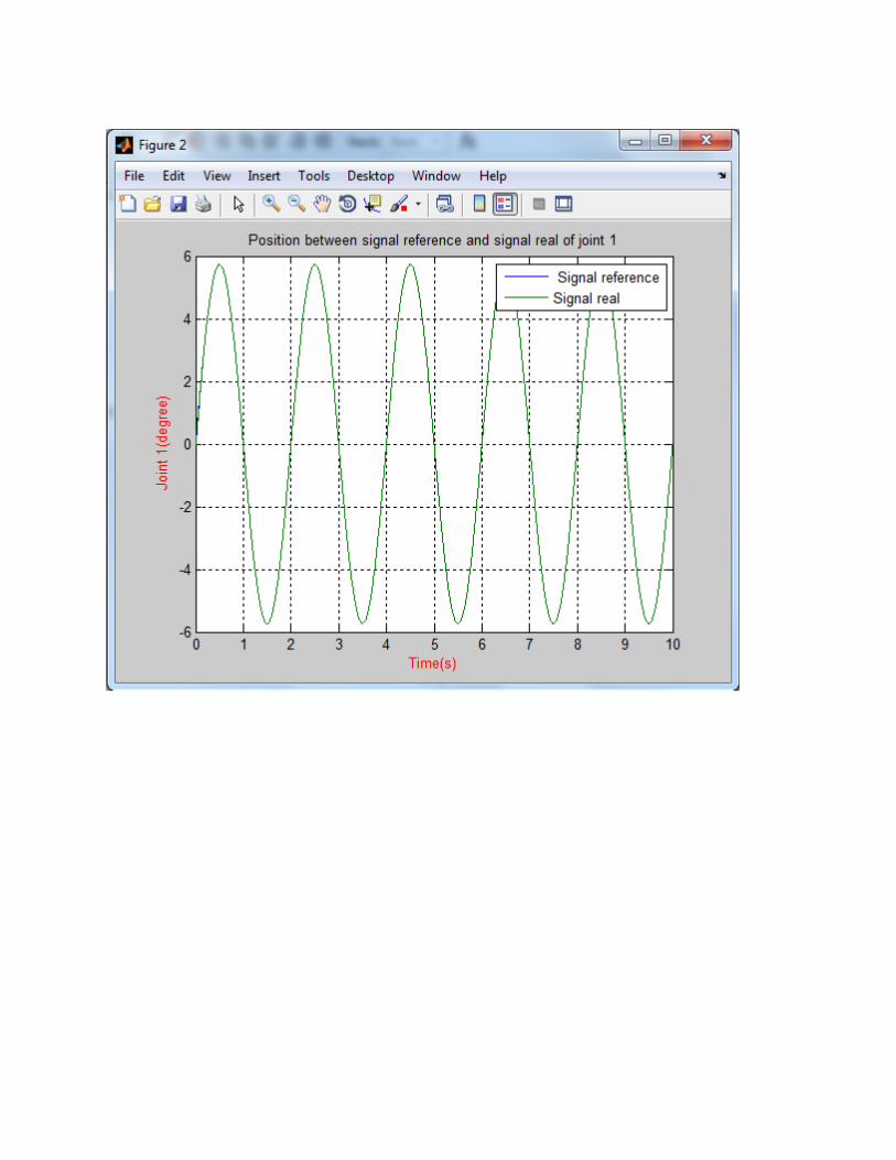
title('Position between signal reference and signal real of joint 1');
legend(' Signal reference','Signal real');
figure(3)
plot(t,qd2*180/pi,t,x(:,2)*180/pi);
grid on;
xlabel('Time(s)','color','r');
ylabel(' Joint 2(degree)','color','r');
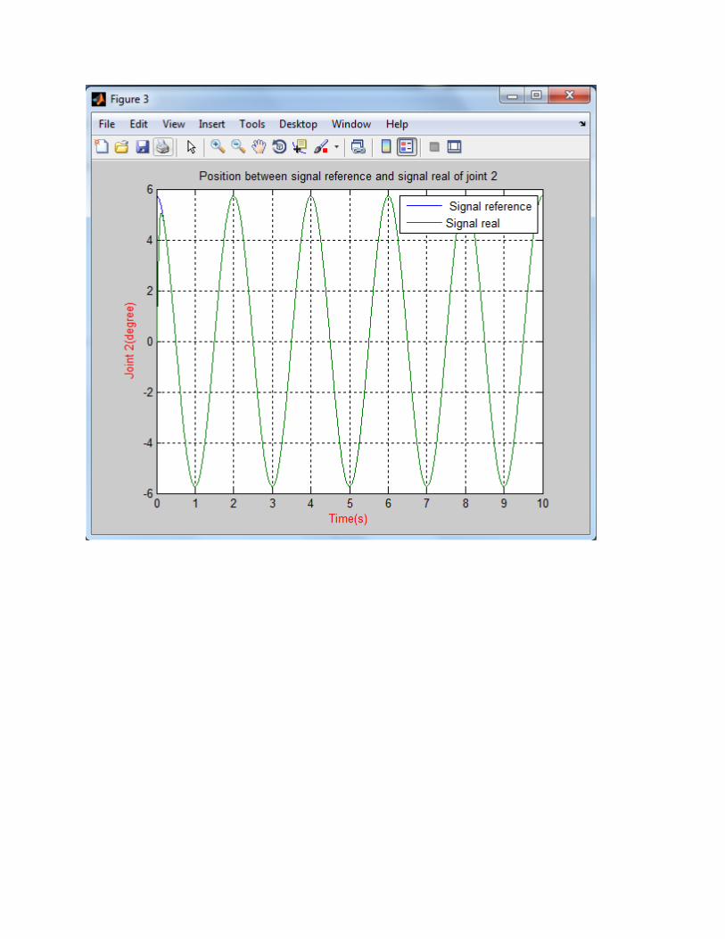
title('Position between signal reference and signal real of joint 2');
legend(' Signal reference','Signal real');
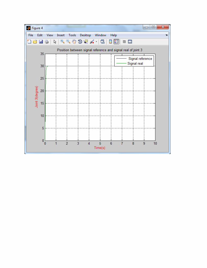
figure(4)
plot(t,qd3*180/pi,t,x(:,3)*180/pi);
grid on;
xlabel('Time(s)','color','r');
ylabel(' Joint 3(degree)','color','r');
title('Position between signal reference and signal real of joint 3');
legend(' Signal reference','Signal real');
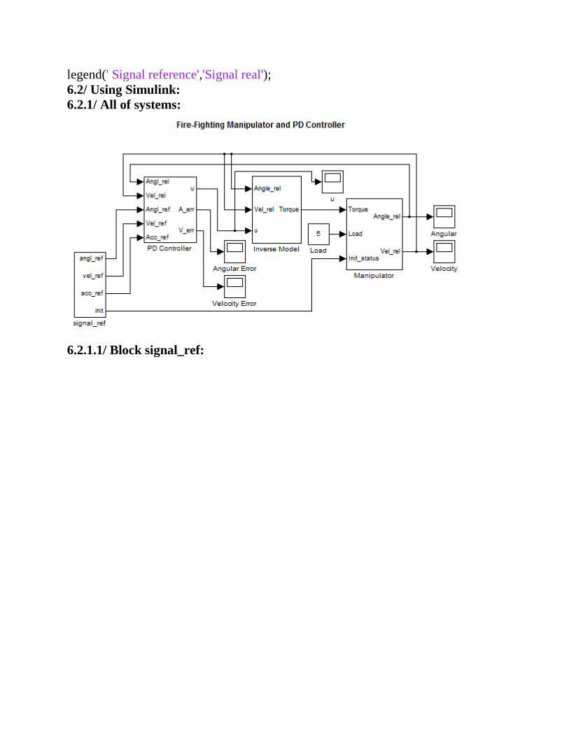
6.2/ Using Simulink:
6.2.1/ All of systems:
6.2.1.1/ Block signal_ref:
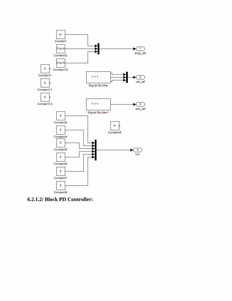
6.2.1.2/ Block PD Controller:
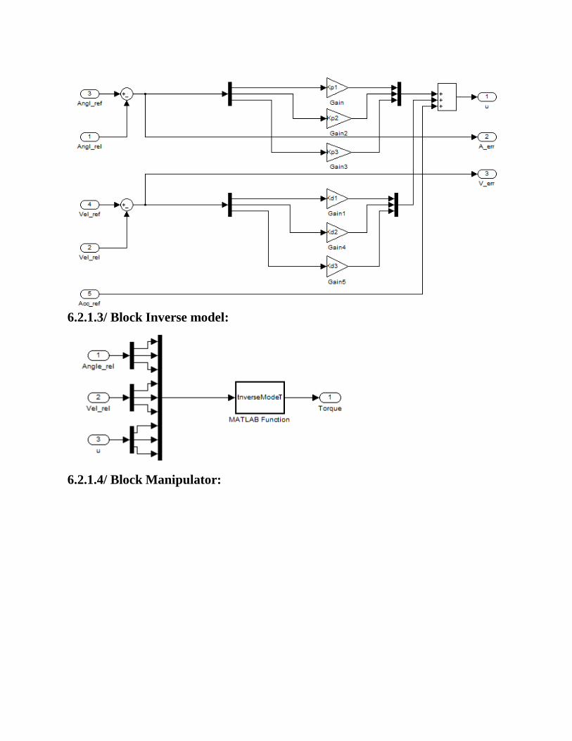
6.2.1.3/ Block Inverse model:
6.2.1.4/ Block Manipulator:
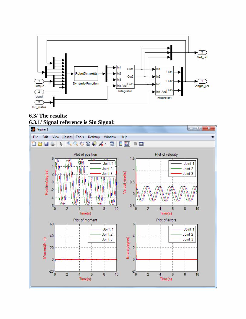
6.3/ The results:
6.3.1/ Signal reference is Sin Signal:
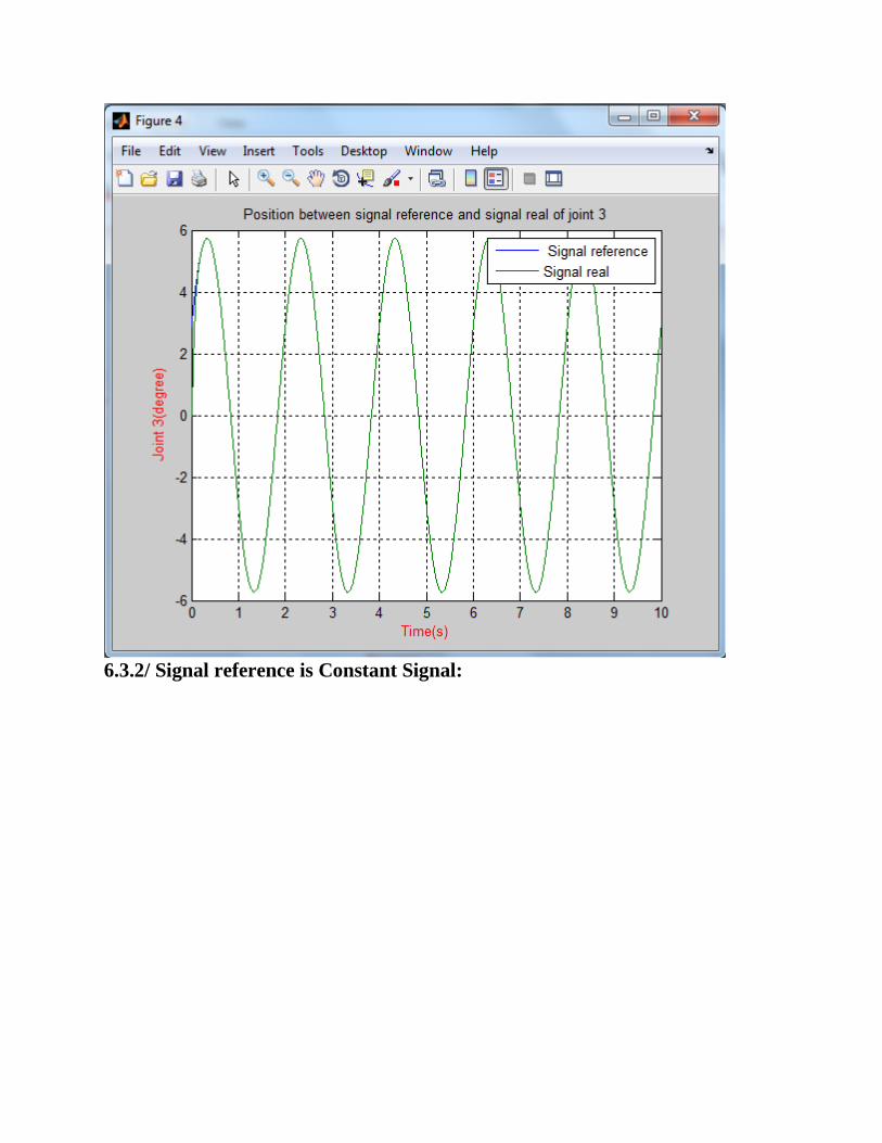
6.3.2/ Signal reference is Constant Signal: