601

Trajectory Planning of a Constrained Flexible Manipulator

Atef A. Ata & Habib Johar

1. Introduction

Many of today’s flexible robots are required to perform tasks that can be considered as constrained motions. A robot is considered to be in constrained maneuvering when its end-effector contacts and/or interacts with the environment as the robot moves. These applications include grinding, deburring, cutting, polishing, and the list continues. For the last two decades many researchers have investigated the constrained motion problem through different techniques such as hybrid position/force control (Raibert, M. & Craig, J., 1981 and Shutter et al., 1996), force control (Su, et al., 1990) , nonlinear modified Corless-Leitman controller (Hu, F. & Ulsoy, G., 1994), two-time scale force position control (Rocco, P. & Book, W., 1996), multi-variable controller (Shi, et al., 1990), parallel force and position control (Siciliano & Villani, L.,2000) , and multi-time-scale fuzzy logic controller (Lin, J., 2003). Luca et al. (Luca, D. & Giovanni, G., 2001) introduced rest-to-rest motion of a two-link robot with a flexible forearm. The basic idea is to design a set of two outputs with respect to which the system has no zero dynamics. Ata and Habib have investigated the open loop performance of a constrained flexible manipulator in contact with a rotary surface (Ata, A. & Habib, J., 2004) and arbitrary shaped fixed surfaces (Ata, A. & Habib, J., 2004). The effect of the contact force on the required joint torques has been simulated for different contact surfaces. Despite the voluminous research done, the study of dynamics and control of the constrained motion of the flexible manipulators remains open for further investigations. The present study aims at investigating the dynamic performance of a constrained rigid/flexible manipulator. The Cartesian path of the end-effector is to be converted into joint trajectories at intermediate points (knots). The trajectory segments between knots are then interpolated by cubic-splines to ensure the smoothness of the trajectory for each joint. To avoid separation between the end-effector and the constraint surface and to minimize the contact surface as well, these knots are chosen at the contact surface itself. Simulation results have been carried out for three contact surfaces. 2. Dynamic Modeling

Consider the two-link planar manipulator shown in Figure (1). The first link is rigid while the second link is flexible and carries a tip mass m3. This tip mass always moves in contact with a constrained surface. The mass density of the flexible link is and Euler-Bernoulli’s beam theory is employed to describe the flexural motion of the flexible link. The manipulator moves in the horizontal plane so that the effect of gravity is not

2ρ

602

considered. The flexible link is described by the Virtual Link Coordinates System (VLCS) in which the deformation is measured relative to the link that joins the end-points and the angle is measured with respect to the horizontal axis (Benati, M. & Morro, A., 1994).

Figure 1. A two link rigid-flexible manipulator with tip mass In general, the dynamic equation of motion for a rigid-flexible robot can be written as:

( ) ( ) r,VM τ+θθ+θθ=τ &&& (1)

where Θ is nx1 vector of joint positions; ⋅

Θ is nx1 vector of joint velocities; ⋅⋅

Θ is nx1 vector

of joint accelerations; M(Θ ) is the nxn inertia matrix; V(Θ ,⋅

Θ ) is the nx1 Coriolis and centripetal terms of the manipulator; τ is the nx1 vector of joint torques, n is the number of degrees of freedom. Based on the dynamical model of an open chain multi-link flexible manipulator using the extended Hamilton’s principle [Ata, A. & Habib, J., 2004 and Benati, M. & Morro, A., 1994], the elements of the inertia and Coriolis matrices of the rigid/flexible manipulator considered here are shown on the appendix .

rτ is the nx1 interaction joint torques due to the force exerted at the end-effector and is given by:

⎥⎦

⎤⎢⎣

⎡==τ

y

xTTr F

FJFJ

where TJ is the transpose Jacobian of the system.

xF and yF represent the applied forces by the end-effector on the constrained surface and it includes two parts. The first component is due to the difference between the proposed coordinates of the end-effector in free motion state and the corresponding point in the contact surface and can be modeled as mass-spring system (Raibert, M. & Craig, J., 1981). The second part arises from the inertia of the tip mass while maneuvering. Then the components of the contact force can be given as:

θ

603

(2)

(3) Where SK is the spring stiffness (N/m), xr , and yr are the coordinates of the contact point. For the second link, the equation due to the flexibility effect can be written as: 0 -)]}-cos()-sin([---{ 2212112

2112

222 =′′′′+ wIElxww θθθθθθθθρ &&&&&&&& (4)

where 22 IE is the flexural stiffness of the flexible link. Equation (4) describes the vibration of the flexible link subject to four boundary conditions:

0)t,0(w = (5a) 0)t,l(w 2 = (5b)

22

2

IE)t(

-)t,0(wτ

=′′ (5c)

0)t,l(w 2 =′′ (5d) 3. Inverse Dynamics Analysis

By introducing a new variable y(x,t) which represents the total deflection of the flexible link as:

)t(x)t,x(w)t,x(y 2θ+= (6) By ignoring the first nonlinear term of equation (4), since its effect is only obvious at very high speed, then equation (4) can be written in terms of y(x,t) as:

0 -)]}-cos()-sin([--{ 22121122

112 =′′′′+ yIEly θθθθθθρ &&&&& (7) The modified boundary conditions are:

0)t,0(y = (8a) )t(l)t,l(y 222 θ= (8b)

22

2

IE)t(

-)t,0(yτ

=′′ (8c)

0)t,l(y 2 =′′ (8d) Solving equation (7) analytically subject to the time-dependent inhomogeneous boundary conditions (8b and c) is quite a difficult task since the flexible torque )(2 tτ that should be obtained is already included in the boundary conditions for the total deflection y(x,t). To avoid this difficulty, )(2 tτ is assumed as the rigid torque without any elastic effect. The boundary condition (8c) can then be evaluated and equations (7) and (6) can be solved to get w(x,t). Finally upon substitution into equation (1) one can get the flexible torque of the

)cossincos

sin()cos-cos-(

22222221

211

11132211

θθθθθθ

θθθθ&&&&

&&

lll

lmllrKF xsx

+++

+=

)cos-sincos-

sin()sin-sin-(

2222222111

12

1132211

θθθθθθ

θθθθ&&&&&

&

lll

lmllrKF ysy

+

+=

604

second link. Using the assumed mode method, the solution for y(x,t) can be assumed in the form (Meirovitch, L., 1967 and Low, K., 1989):

[ ] )t(f)x(h)t(e)x(g)t()x(v)t,x(y nn

�‡

1nn ‡” ++ζ=

= (9) where:

)t(l)t(e 22θ= (10a)

IE)t(-)t(f22

2τ= (10b)

g(x) and h(x) are functions of the spatial coordinate alone to satisfy the homogeneous boundary conditions for )(xvn and they are given by:

x)x(g = (10d)

3

2

22 x

l61-x

21xl

31-)x(h +=

(10e) and )(tnζ is the time function. The subscript n represents the number of modes taking into considerations. In this study, five modes of vibration of the flexible link have been taken into consideration. The corresponding eigenvalue problem for equation (7) can be written:

0)x(vdx

)x(vdk 24

4

2 =ρω+ (11)

Then )(xvn can be obtained using modal analysis in the form (Clough, R. & Penzien, J., 1993):

....3,2,1n,xlnsin

l2)x(v

22n =

πρ

= (12)

The last two nonlinear terms inside the parentheses in equation (6) can be regarded as distributed excitation force with unit density. This effect can be compensated for the time function as (Meirovitch, L., 1967 and Low, K., 1989):

τττω

ζ dtNtt

nn

n )-sin(1 )(0∫= (13)

The convolution integral in equation (13) can be evaluated using Duhamel integral method (Clough, R. & Penzien, J., 1993). Then, the rigid and flexible torques incorporated with vibration effects can be obtained from equations (1). 4. Model Verification

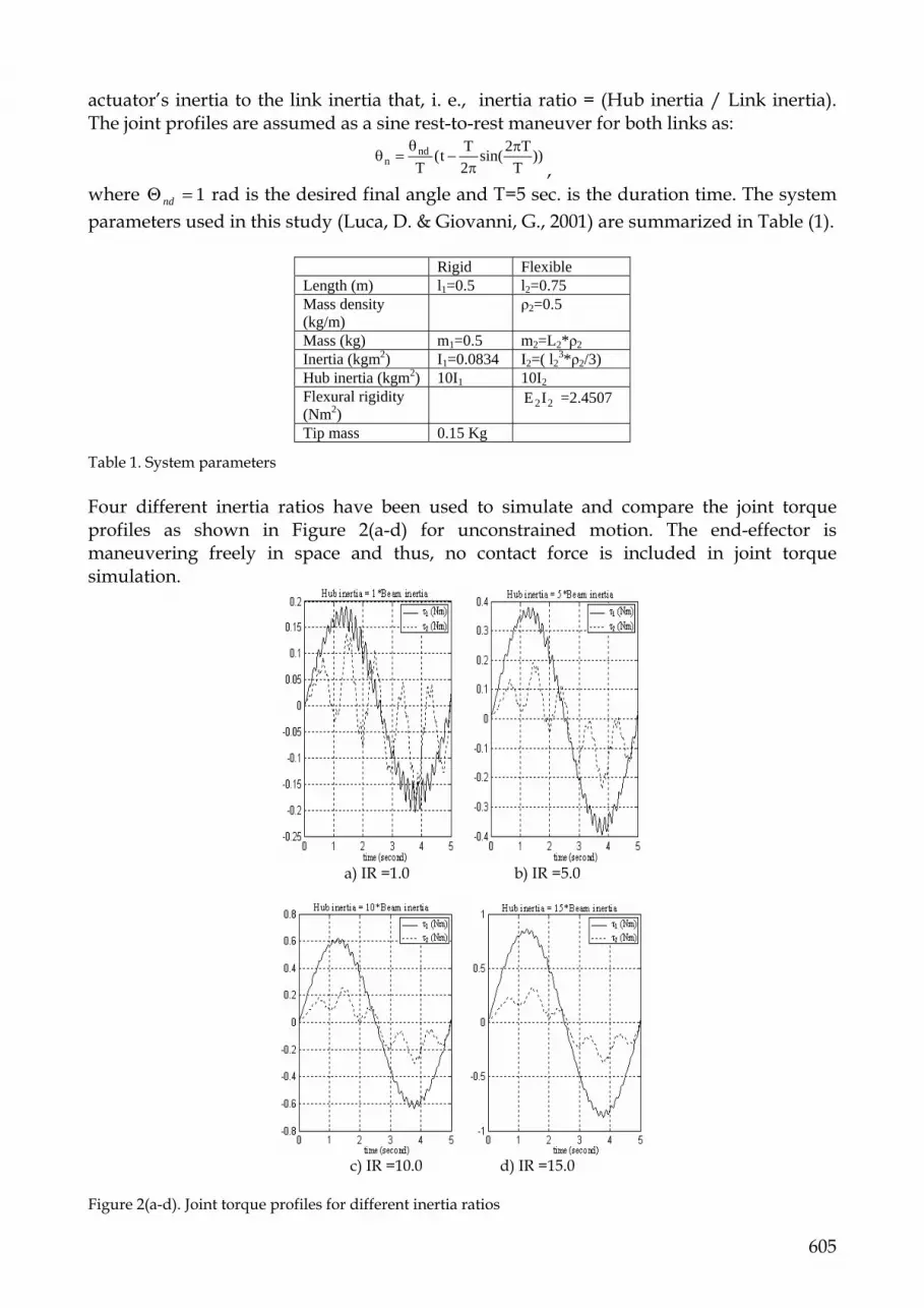
To verify the proposed dynamical model a simulation of the joint torques through the solution of the inverse dynamics problem has been carried out for different values of the hub to beam inertia ratio (IR). The inertia ratio is defined as the percentage of the

605

actuator’s inertia to the link inertia that, i. e., inertia ratio = (Hub inertia / Link inertia). The joint profiles are assumed as a sine rest-to-rest maneuver for both links as:

))T

T2sin(2Tt(

Tnd

nπ

π−

θ=θ

, where 1=Θnd rad is the desired final angle and T=5 sec. is the duration time. The system parameters used in this study (Luca, D. & Giovanni, G., 2001) are summarized in Table (1). Table 1. System parameters Four different inertia ratios have been used to simulate and compare the joint torque profiles as shown in Figure 2(a-d) for unconstrained motion. The end-effector is maneuvering freely in space and thus, no contact force is included in joint torque simulation.

a) IR =1.0 b) IR =5.0

c) IR =10.0 d) IR =15.0

Figure 2(a-d). Joint torque profiles for different inertia ratios

Rigid Flexible Length (m) l1=0.5 l2=0.75 Mass density (kg/m)

ρ2=0.5

Mass (kg) m1=0.5 m2=L2*ρ2 Inertia (kgm2) I1=0.0834 I2=( l2

3*ρ2/3) Hub inertia (kgm2) 10I1 10I2 Flexural rigidity (Nm2)

22IE =2.4507

Tip mass 0.15 Kg

606

It is clear from Figure 2(a-d) that fluctuations arise in joint torques due to the vibrations of flexible link while the manipulator is maneuvering. As the inertia ratio increases, the magnitude of the joint torques increases and the amplitudes of fluctuations decrease. It should be noticed that the amplitudes of fluctuations in joint torques resulting from inertia ratio of 10 have significantly diminished as compared to those of inertia ratio of 1 and 5. This implies that vibration effects on joint torques can be damped to certain extent with a good selection of inertia ratio. The situation is even better for an inertia ratio of 15 where the fluctuations are very much significantly reduced but the price is a bigger actuator size. However, since we desire to design light weight manipulator, inertia ratio of 10 is more preferable to that of 15. This conforms with the stability analysis of stable and asymptotically stable flexible manipulator (Ata, et al., 1996). 5. Cubic-Spline Trajectory Interpolations

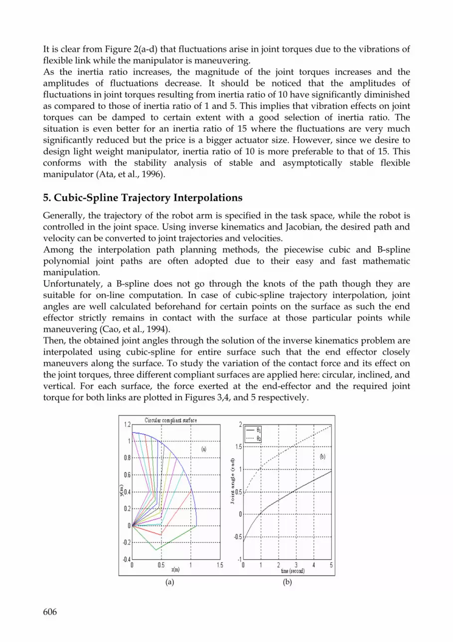
Generally, the trajectory of the robot arm is specified in the task space, while the robot is controlled in the joint space. Using inverse kinematics and Jacobian, the desired path and velocity can be converted to joint trajectories and velocities. Among the interpolation path planning methods, the piecewise cubic and B-spline polynomial joint paths are often adopted due to their easy and fast mathematic manipulation. Unfortunately, a B-spline does not go through the knots of the path though they are suitable for on-line computation. In case of cubic-spline trajectory interpolation, joint angles are well calculated beforehand for certain points on the surface as such the end effector strictly remains in contact with the surface at those particular points while maneuvering (Cao, et al., 1994). Then, the obtained joint angles through the solution of the inverse kinematics problem are interpolated using cubic-spline for entire surface such that the end effector closely maneuvers along the surface. To study the variation of the contact force and its effect on the joint torques, three different compliant surfaces are applied here: circular, inclined, and vertical. For each surface, the force exerted at the end-effector and the required joint torque for both links are plotted in Figures 3,4, and 5 respectively.

(a) (b)

607

(c) (d)

Figure 3. Circular surface: (a) End-effector trajectory, (b) Joint angles (c) Force distribution (d) Joint torques profiles

(a) (b)

(c) (d)

Figure 4. Inclined Surface: (a) End-effector trajectory, (b) Joint angles (c) Force distribution (d) Joint torques profiles

608

(a) (b)

(c) (d)

Figure 5. Vertical surface: (a) End-effector trajectory, (b) Joint angles (c) Force distribution (d) Joint torques profiles Simulation of force distribution in Figures 3(c), 4(c) and 5(c) verifies that designing the joint trajectories based on cubic-splines ensures that the end effector closely maneuvers along the desired trajectory. However, in the case of circular contact surface, the initial force distribution in Figure 3(a) is relatively high within the time interval of 0 to 1 second and then gradually reduces as the end effector moves along the surface. This force is expected to be small since the end-effector is controlled to pass closely to the constraint surface. This implies that the cubic-spline interpolation technique may have a good command on the end-effector to maneuver closely along the entire contact surface only for certain shapes of surface. Perhaps for complicated shapes of contact surface, the cubic-spline interpolation technique may not work well to compel the end effector to maneuver closely along the entire region of the contact surface. The simulation of the joint torque profiles in Figures 3(b), 4(b) and 5(b) shows that irregular fluctuations can appear in the joint torque profiles due to the effect of cubic-spline interpolation. 6. Conclusions

Constrained motion of a planar rigid-flexible manipulator is considered in this study. a dynamic model with zero tip deformation constraint of constrained rigid-flexible

609

∫=2

0222

l

xdxxm ρ

manipulator moving in horizontal plane is derived. A systematic approach of analytic solution to the fourth order differential equation with time dependent, nonhomogeneous boundary conditions including the nonlinear terms is presented to compute the elastic deflection w(x,t) of the flexible link while maneuvering. The joint motion profiles have been designed based on the cubic-splines interpolation to ensure that the end-effector will move along the constrained surface without separation. The proper hub to beam inertia ratio of 10 has been selected based on a comparison study 7. Appendix

Equations of motion

)lmlmII(M 213

2121h111 +++=

)-cos()( 1221321212 θθllmxlmM +=

∫ Θ−Θ−2

0121 )sin(

l

dxwlρ

1221 MM =

∫++++=2

0

222332222 )(

l

h dxwlmIIIM ρ

∫++=2

012212

221212

2221321211 )]-sin()(2-)-cos()-[()-sin()(-

l

dxwwwlllmxlmv θθθθθθρθθθ &&&&&&

∫ ++++=2

012

2112212

2121321221 )}-cos(2-{)-sin()(

l

dxwlwxwwllmxlmv θθθθρθθθ &&&&&&

where and and are the inertia of the links and actuators respectively.

⎟⎟⎠

⎞⎜⎜⎝

⎛θθ

θ+θθθ=

2222

22112211T

cosl sinl-coslcosl sinl-sinl-

J

8. References

Atef A. Ata & Habib Johar (2004) “ Dynamic Analysis of a Rigid-Flexible Manipulator constrained by Arbitrary Shaped Surfaces”, International Journal of Modelling and Simulation, To appear soon.

Atef A. Ata & Habib Johar (2004) “Dynamic simulation of task constrained of a rigid-flexible manipulator”, International Journal of Advanced Robotic Systems, Vol. 1, No. 2, June 2004, pp. 61-66.

Atef, A. Ata , Salwa M. Elkhoga, Mohamed A. Shalaby, & Shihab S. Asfour (1996) “ Causal inverse dynamics of a flexible hub- arm system through Liapunov second method” Robotica Vol. 14, pp 381-389.

Benati, M. & Morro, A. (1994). Formulation of equations of motion for a chain of flexible links using Hamilton’s principle. ASME J. Dynamic System, Measurement and Control , 116, pp. 81-88.

Cao, B., Dodds, G. I., & Irwin, G. W.(1994). Time Optimal and Smooth Constrained Path Planning for Robot Manipulators. Proceeding of IEEE International Conference on Robotics and Automation, pp. 1853-1858.

nI hnI

610

Clough, R.W. & Penzien, J. (1993). Dynamics of Structures, McGraw-Hill, Inc.,. Hu, F. L. & Ulsoy, G. (1994). Force and motion control of a constrained flexible robot arm.

ASME, J. Dynamic System, Measurement and Control, 116, pp. 336-343. Lin, J. (2003). Hierarchical fuzzy logic controller for a flexible link robot arm performing

constrained motion task, IEE Proceedings: Control Theory and Applications, Vol. 150, No. 4, , pp. 355-364.

Low, K. H.(1989). Solution schemes for the system equations of flexible robots. J. Robotic Systems, 6, pp. 383 -405.

Luca, D. A. & Giovanni, D. G. (2001). Rest-to-Rest motion of a two-link robot with a flexible forearm. IEEE/ASME Int. Conf. on Advanced Intelligent Mechatronics, pp. 929-935.

Meriovitch, L. (1967). Analytical Methods in Vibrations. The Macmillan Co., New York. Raibert, M. H. & Craig ,J. J. (1981). Hybrid position / force control of manipulator, ASME

J. of Dyanmics Systems, Measurement and Control, 102, pp. 126-133. Rocco P. P & Book, W. J. (1996). Modeling for two-time scale force/position control of

flexible arm. IEEE Proc. International conference on Robotics and Automation, pp. 1941-1946.

Schutter , J. D., Torfs, D. & Bruyninckx , H. (1996). Robot force control with an actively damped flexible end-effector. J. Robotics and Autonomous System, 19, pp. 205-214.

Shi, Z. X., Fung, E. H. K., and Li, Y. C. (1999). Dynamic modeling of a rigid-flexible manipulator for constrained motion task control. J. Applied Mathematical Modeling 23, pp. 509-529.

Siciliano & Villani, L. (2000). Parallel force and position control of flexible manipulators. IEE Proc-Control Theory Appl. 147, pp. 605 -612.

Su, H. J., Choi, B. O. & Krishnamurty , K. (1990). Force control of high-speed, lightweight robotic manipulator. Mathl. Comput. Modeling 14, pp. 474 -479.