Fire modelling in computational fluid dynamics (CFD)

Dr. Andrej HorvatIntelligent Fluid Solutions Ltd.

NAFEMS Webinar Series

26 May 2010

Fire Modelling in Computational Fluid

Dynamics (CFD)

Fire Modelling in Computational Fluid

Dynamics (CFD)

2

IFSIFSOverview of fluid dynamics transport equations- transport of mass, momentum, energy and composition

- influence of convection, diffusion, volumetric (buoyancy) force

- transport equation for thermal radiation

Averaging and simplification of transport equations- spatial and time averaging

- influence of averaging on zone and field models

- solution methods

CFD modelling- turbulence models (k-epsilon, k-omega, Reynolds stress, LES)

- combustion models (mixture fraction, eddy dissipation, flamelet)

- thermal radiation models (discrete transfer, Monte Carlo)

Conclusions

Contents

3

IFSIFSToday, CFD methods are well established tools that help in design, prototyping, testing and analysis

The motivation for development of modelling methods (not only CFD) is to reduce cost and time of product development, and to improve efficiency and safety of existing products and installations

Verification and validation of modelling approaches by comparing computed results with experimental data is necessary

Experimental investigation of fire in a realistic environment is in many situations impossible. In such cases, CFD is the only viable analysis and design tool.

Introduction

4

IFSIFSFire modelling is an area of computational modelling which aims to predict fire behaviour in different environmental conditions.

Therefore, these computational models need to take into account fluid dynamics, combustion and heat transfer processes.

The complexity of the fire modelling arises from significantly different time scales of the modelled processes. Also, not completely understood physics and chemistry of fire adds the uncertainty to the modelling process.

Introduction

5

IFSIFS

Overview of fluid dynamics

transport equations

6

IFSIFSTransport equations

Eulerian and Lagrangian description

Eulerian description – transport equations for mass, momentumand energy are written for a (stationary) control volume

Lagrangian description – transport equations for mass, momentum and energy are written for a moving material particle

7


Majority of the numerical modelling in fluid mechanics is based on the Eulerian formulation of transport equations

Using the Eulerian formulation, each physical quantity is described as a mathematical field. Therefore, these models are also named field models

Lagrangian formulation is a basis for particle dynamics modelling: bubbles, droplets (sprinklers), solid particles (dust) etc.

8


Droplets trajectories from sprinklers (left), gas temperature field during fire suppression (right)

9

IFSIFSThe following physical laws and terms also need to be included

- Newton's viscosity law - Fourier's law of heat conduction- Fick's law of mass transfer

- Sources and sinks due to thermal radiation, chemical reactions etc.

Transport equations

} diffusive terms -flux is a linear function of a gradient

10

IFSIFSTransport of mass and composition

Transport of momentum

Transport of energy

Transport equations

( ) Mviit =ρ∂+ρ∂ ( ) ( ) ( ) jjiijiijt MDv +ξ∂ρ∂=ρξ∂+ρξ∂

( ) ( ) ( ) jjijijjiijt FgSpvvv +ρ+μ∂+−∂=ρ∂+ρ∂ 2 ( )jiijij vvS ∂+∂=2

1

( ) ( ) ( ) QThvh iiiit +∂λ∂=ρ∂+ρ∂

change in a control vol. flux difference

(convection)

diffusion

volumetric term

11


Lagrangian formulation is simpler

- particle location equation

- mass conservation eq. for a particle

- momentum conservation eq. for a particle

- thermal energy conservation eq. for a particle

Transport equations of the Lagrangianmodel need to be solved for each representative particle

udtxdrr =

( ) VLD FFFdtudmrrrr ++=

Mdtdm =

volumetric forces

drag lift

( ) RLCp QQQdtdTmc ++=

thermal radiation

convection latent heat

12

IFSIFSThermal radiation

Equations describing thermal radiation are much more complicated

- spectral dependency of material properties- angular (directional) dependence of the radiation transport

Transport equations

( ) ( ) ( ) ( ) ( )∫π

ννν

νννννν ΩΩ→ΩΩ

π++Ω+−=Ω

44'd'P'I

KIKIKK

ds

dIs

seasa

in-scatteringchange of radiationintensity

absorption and

out-scattering

emission

13

IFSIFS

Averaging and simplification

of transport equations

14

IFSIFSAveraging and simplification of transport equations

The presented set of transport equations is analytically unsolvable for majority of cases

Success of a numerical solving procedure is based on density of the numerical grid, and in transient cases, also on the size of the integration time-step

Averaging and simplification of transport equations help (and improve) solving the system of equations:

- derivation of averaged transport equations for turbulent flow simulations

- derivation of integral (zone) models

15

IFSIFSAveraging and simplification of transport equations

Averaging and filtering

The largest flow structures can occupy the whole flow field, whereas the smallest vortices have the size of Kolmogorov scale

ρ, vi , p, h

χ,τw

( )4

13 εν=η ( )4

1

εν=ηu ( )2

1

εν=τη

16

IFSIFSKolmogorov scale is (for most cases) too small to be captured with a numerical grid

Therefore, the transport equations have to be filtered(averaged) over:

- spatial interval → Large Eddy Simulation (LES) methods

- time interval → k-epsilon model, SST model, Reynolds stress models

Averaging and simplification of transport equations

17

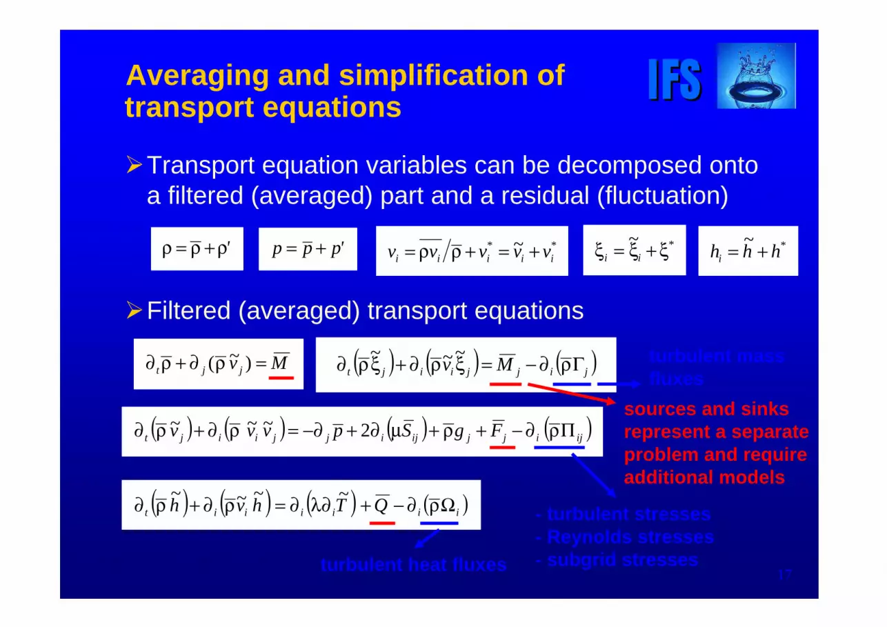
IFSIFSTransport equation variables can be decomposed onto a filtered (averaged) part and a residual (fluctuation)

Filtered (averaged) transport equations

*ii

*iii vv~vvv +=+ρρ='ρ+ρ=ρ 'ppp += *

i hh~

h +=

Mv~jjt =ρ∂+ρ∂ )(

( ) ( ) ( ) ( )ijijjijijjiijt FgSpv~v~v~ Πρ∂−+ρ+μ∂+−∂=ρ∂+ρ∂ 2

( ) ( ) ( ) ( )iiiiiit QT~

h~

v~h~ Ωρ∂−+∂λ∂=ρ∂+ρ∂

( ) ( ) ( )jijjiijt M~

v~~ Γρ∂−=ξρ∂+ξρ∂

*ii

~ ξ+ξ=ξ

sources and sinks represent a separate problem and require additional models

- turbulent stresses- Reynolds stresses- subgrid stressesturbulent heat fluxes

turbulent mass fluxes


18

IFSIFS

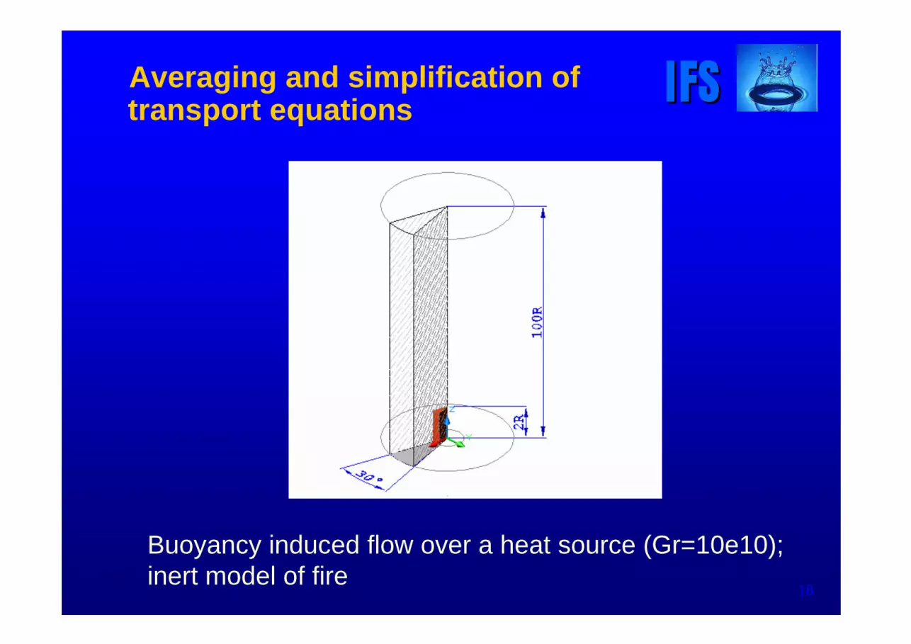
Buoyancy induced flow over a heat source (Gr=10e10);inert model of fire


19

IFSIFS

LES model; instantaneous temperature field


20

IFSIFS

a) b)

Temperature field comparison: a) steady-state RANS model, b) averaged LES model results


21

IFSIFSAdditional simplifications

- flow can be modelled as a steady-state case → the solution is a result of force, energy and mass flow balancetaking into consideration sources and sinks

- fire can be modelled as a simple heat source → inert firemodels; do not need to solve transport equations for composition

- thermal radiation heat transfer is modelled as a simple sinkof thermal energy → FDS takes 35% of thermal energy

- control volumes can be so large that continuity of flow properties is not preserved → zone models


22

IFSIFS

CFD Modelling

23

IFSIFSTurbulence models

laminar flow

transitional flow

turbulent flow

van Dyke, 1965

24

IFSIFSTurbulence models introduce additional (physically related) diffusion to a numerical simulation

This enables :

- RANS models to use a larger time step (Δt >> Kolmogorovtime scale) or even a steady-state simulation

- LES models to use a less dense (smaller) numerical grid(Δx > Kolmogorov length scale)

The selection of the turbulence model fundamentally influences distribution of the simulated flow variables (velocity, temperature, heat flow, composition etc)

Turbulence models

25

IFSIFSIn general, 2 kinds of averaging (filtering) exist, which leads to 2 families of turbulence models:

- filtering over a spatial interval → Large Eddy Simulation(LES) models

- filtering over a time interval → Reynolds Averaged Navier-Stokes (RANS) models: k-epsilon model, SST model, Reynolds Stress models etc

For RANS models, size of the averaging time interval is not known or given (statistical average of experimental data)

For LES models, size of the filter or the spatial averaging interval is a basic input parameter (in most cases, it is equal to grid spacing)

Turbulence models

26


Reynolds Averaged Navier-Stokes (RANS) models

For two-equation models (e.g. k-epsilon, k-omega or SST), 2 additional transport equations need to be solved:

- for kinetic energy of turbulent fluctuations

- for dissipation of turbulent fluctuations

or

- for frequency of turbulent fluctuations

These variables are then used to calculate eddy viscosity:

)( *ij

*ij vv ∂∂μ=ερ

k~ εω

iik Π= 21

ω=

ε=μ μ

kρkρCt

2

27

IFSIFSReynolds Averaged Navier-Stokes (RANS) models

- from eddy viscosity, Reynolds stresses, turbulent heat and mass fluxes are obtained

- model parameters are usually defined from experimental data e.g. dissipation of grid generated turbulence or flow in a channel

- transport equation for k is derived directly from the transport equations for Reynolds stresses

- transport equation for ε is empirical

Turbulence models

h~

Pr jt

tj ∂μ−=Ωρ

jilltijtjillij v~S δ∂μ+μ−=δΠρ−Πρ )(3

22

3

1 ξ∂μ−=Γρ ~

cS jt

tj

ijΠ

28


Large Eddy Simulation (LES) models

- Large Eddy Simulation (LES) models are based on spatial filtering (averaging)

- many different forms of the filter exist, but the most common is "top hat" filter (simple geometrical averaging)

- size of the filter is based on a grid node spacing

Basic assumption of LES methodology:

Size of the used filter is so small that the averaged flow structures do no influence large structures, which do contain most of the energy.

These small structures are being deformed, disintegrated onto even smaller structures until they do not dissipate due to viscosity (kinetic energy → thermal energy).

29



- eddy (turbulent) viscosity is defined as

where

- using the definition of turbulence (subgrid) stresses

and turbulence fluxes

the expression for eddy viscosity can be written as

where the contributiondue to buoyancy is

jilltijtjiji v~Sk δ∂μ+μ−=δρ−Πρ )(3

22

3

2

3134 //t l~ ερμ ΔsC~l

h~

Pr jt

tj ∂μ−=Ωρ

( ) ( ) 212 2 /ijjist GSSC +Δρ=μ

h~

Pr

h~

g~G

t

ii∂

grid spacing

30



- presented Smagorinsky model is the simplest from the LES models

- it requires knowledge of empirical parameter Cs, which is not constant for all flow conditions

- newer, dynamic LES models calculate Cs locally - the procedure demands introduction of the secondary filter

- LES models demand much denser (larger) numerical grid

- they are used for transient simulations

- to obtain average flow characteristics, we need to perform statistical averaging over the simulated time interval

31


Comparison of turbulence models

25 50 75 100

z/R

1

2

3

4

5

678

wc(

R/F

0)1

/3

k-e (Gr = 10 10)k-e N&B (Gr = 1010)RNG k-e (Gr = 1010)S S T (Gr = 1010)S S G (Gr = 1010)LES (Gr = 1010)Rous e e t al. (1952)S habbir and Ge orge (1994)

25 50 75 100

z/R

10-2

10-1

bc(

R5/F

02)1

/3

k-e (Gr = 10 10)k-e N&B (Gr = 1010)RNG k-e (Gr = 1010)S S T (Gr = 1010)S S G (Gr = 1010)LES (Gr = 10 10)Rous e e t al. (1952)S habbir and George (1994)

a) b)

Buoyant flow over a heat source: a) velocity, b) temperature*

32

IFSIFSCombustion models

Chen et al., 1988

Grinstein,Kailasanath, 1992

33

IFSIFSCombustion can be modelled with heat sources

- information on chemical composition is lost - thermal loading is usually under-estimated

Combustion modelling contains

- solving transport equations for composition

- chemical balance equation

- reaction rate model

Modelling approach dictates the number of additional transport equations required

Combustion models

34

IFSIFSModelling of composition requires solving n-1 transport equations for mixture components – mass or molar(volume) fractions

Chemical balance equation can be written as

or

Combustion models

( ) ( ) jjit

tijiijt M

~

ScSc

~v~

~ +⎟⎟⎠

⎞⎜⎜⎝

⎛ξ∂⎟⎟

⎠

⎞⎜⎜⎝

⎛ μ+μ∂=ξρ∂+ξρ∂

.....C"B"A".....C'B'A' CBACBA ν+ν+ν↔ν+ν+ν

I"I'N

....C,B,AII

N

....C,B,AII ∑∑

==

ν↔ν

35

IFSIFSReaction source term is defined as

or for multiple reactions

where R or Rk is a reaction rate

Reaction rate is determined using different models

- Constant burning (reaction) velocity- Eddy break-up model and Eddy dissipation model- Finite rate chemistry model- Flamelet model- Burning velocity model

Combustion models

( )R'"WM jjjj ν−ν= ( )∑ ν−ν=k

kj,kj,kjj R'"WM

36

IFSIFSConstant burning velocity sL

speed of flame front propagation islarger due to expansion

- values are experimentally determined for ideal conditions

- limits due to reaction kinetics and fluid mechanics are not taken into account

- source/sink in mass fraction transport equation

- source/sink in energy transport equation

- expressions for sL usually include additional models

Combustion models

Lh

cF ss

ρρ=

ls~M Lfj ρ

cj hM~Q Δ

37

IFSIFSEddy break-up model and Eddy dissipation model

- is a well established model that can be used for simple reactions (one- and two-step combustion)

- in general, it cannot be used for prediction of products of complex chemical processes (NO, CO, SOx, etc)

- it is based on the assumption that the reaction is much faster than the transport processes in flow

- reaction rate depends on mixing rate of reactants in turbulent flow

- Eddy dissipation model reaction rate

Combustion models

k~sL ε

( ) ⎟⎟⎠

⎞⎜⎜⎝

⎛

+ψψψερ=

s

~C,

s

~,~

kCR p

Bo

fA1

min

38

IFSIFSBackdraft simulation

Combustion models

Horvat et al., 2008

inflow of fresh air

outflow of comb.products

fireball

39

IFSIFSFinite rate chemistry model

- it is applicable when a chemical reaction rate is slow or comparable with turbulent mixing

- reaction kinetics must be known

- for each additional reaction the same expression is added

- the model is numerically demanding due to exponential terms

- often the model is used in combination with the Eddy dissipation model

Combustion models

∏=

νβ ψ⎟⎠⎞

⎜⎝⎛ −=

...C,B,AI

'I

a I~T~

R

EexpT

~AR

40

IFSIFSFlamelet model

- describes interaction of reaction kinetics with turbulent structures for a fast reaction (high Damköhler number)

- basic assumption is that combustion is taking place in thin sheets - flamelets

- turbulent flame is an ensemble of laminar flamelets

- the model gives a detailed picture of the chemical composition - resolution of small length and time scales of the flow is not needed

- the model is also known as "Mixed-is-burnt" - large difference between various implementations of the model

Combustion models

41


- it is based on definition of a mixture fraction

or where

- the conditions in vicinity of flamelets are described with the respect to Z; Z=Zst is a surface with the stoihiometricconditions

- transport equations are rewritten with Z dependencies;conditions are one-dimensional ξ(Z) , T(Z) etc.

Combustion models

Z kg/s fuel

BA

BMZβ−ββ−β=

mixingproces

1 kg/s mixture

1-Z kg/s oxidiser

( ) MBA ZZ β=β−+β 1

A

BM

iof ξ−ξ=β

42


- for turbulent flow, we need to solve an additional transport equation for mixture fraction Z

- and a transport equation for variation of mixture fraction Z"

- composition is calculated from preloaded libraries

Combustion models

( ) ( ) ⎟⎟⎠

⎞⎜⎜⎝

⎛∂⎟⎟⎠

⎞⎜⎜⎝

⎛ μ+μ∂=ρ∂+ρ∂ Z~

ScScZ~

v~Z~

it

tiiit

( )~

Zk

CZ~

ScZ

ScDZu~Z ''

it

t''i

t

ti

''ii

''t

~~22222 2

ερ−∂μ+⎪⎭

⎪⎬⎫

⎪⎩

⎪⎨⎧

∂⎟⎟⎠

⎞⎜⎜⎝

⎛ μ+ρ∂=⎟⎟⎠

⎞⎜⎜⎝

⎛ρ∂+⎟⎟⎠

⎞⎜⎜⎝

⎛ρ∂ χ

~

( ) ( )dZZPDFZ~jj ∫ψ=ψ

1

0

( ) ( ) ( ) χχχψ=ψ ∫ ∫∞

ddZPDFZPDF,Z~jj

1

0 0

these PDFs are tabulated for different fuel, oxidiser, pressure and temperature

43

IFSIFSIt is a very important heat transfer mechanism in fires

In fire simulations, thermal radiation should not be neglected

The simplest approach is to reduce the heat release rate of a fire (35% reduction in FDS)

Modelling of thermal radiation - solving transport equation for radiation intensity

( ) ( ) ( ) ( ) ( )∫π

ννν

νννννν ΩΩ→ΩΩ

π++Ω+−=Ω

44'd'P'I

KIKIKK

ds

dIs

seasa

Thermal radiation

in-scatteringchange of intensity

absorption and scattering

emission

44

IFSIFSRadiation intensity is used for definition of a source/sink in the energy transport equation and radiation wall heat fluxes

Energy spectrum of blackbody radiation

ν - frequencyc - speed of lightn - refraction indexh - Planck's constantkB - Boltzmann's constant

integration over the whole spectrum

Thermal radiation

( ) ( ) ( ) ]Hz[Wm1

2 1-2-2

2

2

−ννπν=π= νν Tkhexp

hn

cTITE

B

( ) ( ) ][Wm 2-

0

42 ν=σ= ∫∞

ν dTETnTE

45

IFSIFSDiscrete Transfer

- modern deterministic model- assumes isotropic scattering, homogeneous gas properties- each wall cell works as a radiating surface that emits raysthrough the surrounding space (separated onto multiple solid angles)

- radiation intensity is integrated along each ray between the walls of the simulation domain

- source/sink in the energy transport equation

Thermal radiation

( ) ( ) νν−

ν+

νν +−+= νν IKeIIs,rI ssK

esKK asa 1e)( -

0

( )∫π

νν Ωθϕ=4

dcoscoss,rIq jrad

j,

radii

rad qQ −∂=

46

IFSIFSMonte Carlo

- it assumes that the radiation intensity is proportional to (differential angular) flux of photons

- radiation field can be modelled as a "photon gas" - absorption constant Kaν is the probability per unit length of

photon absorption at a given frequency ν- average radiation intensity Iν is proportional to the photon

travelling distance in a unit volume and time- radiation heat flux qrad is proportional to the number of

photon incidents on the surface in a unit time

- accuracy of the numerical simulation depends on the number of used "photons"

Thermal radiation

47

IFSIFSThese radiation methods can be used:

- for an averaged radiation spectrum - grey gas

- for a gas mixture, which can be separated onto multiple grey gases (such grey gas is just a modelling concept)

- for individual frequency bands; physical parameters are very different for each band

Thermal radiation

48

IFSIFSFlashover simulation

Thermal radiation

Horvat et al., 2009

propane burner

wooden targets

primary fire

secondary fire

49

IFSIFS

Conclusions

50

IFSIFSThe webinar gave a short (but demanding) overview of fluid mechanics and heat transfer theory that is relevant for fire simulations

All current commercial CFD software packages (ANSYS-CFX, ANSYS-Fluent, Star-CD, Flow3D, CFDRC, AVL Fire) contain most of the shown models and methods:

- they are based on the finite volume or the finite element method and they use transport equations in their conservative form

- numerical grid is unstructured for greater geometrical flexibility

- open-source computational packages exist and are freely accessible (FDS, OpenFoam, SmartFire, Sophie)

Conclusions

51

IFSIFSAndrej Horvat

Intelligent Fluid Solutions Ltd.99 Milton Park, Abingdon, Oxfordshire, OX14 4RY, UK

Tel.: +44 (0)1235 841 505Fax: +44 (0)1235 854 001Mobile: +44 (0)78 33 55 63 73Skype: a.horvat E-mail: [email protected]: www.intelligentfluidsolutions.co.uk

Contact information

Documents

Fire modelling in computational fluid dynamics (CFD)