First Results from the CHARA Array. VII. Long‐Baseline Interferometric Measurements of Vega Consistent with a Pole‐On, Rapidly Rotating Star

FIRST RESULTS FROM THE CHARA ARRAY. VII. LONG-BASELINE INTERFEROMETRIC MEASUREMENTSOF VEGA CONSISTENT WITH A POLE-ON, RAPIDLY ROTATING STAR

J. P. Aufdenberg,1,2

A. Merand,3V. Coude du Foresto,

3O. Absil,

4E. Di Folco,

3P. Kervella,

3S. T. Ridgway,

2,3

D. H. Berger,5,6

T. A. ten Brummelaar,6H. A. McAlister,

7J. Sturmann,

6L. Sturmann,

6and N. H. Turner

6

Received 2006 January 5; accepted 2006 March 9

ABSTRACT

We have obtained high-precision interferometric measurements of Vega with the CHARA Array and FLUORbeam combiner in the K 0 band at projected baselines between 103 and 273 m. The measured visibility amplitudesbeyond the first lobe are significantly weaker than expected for a slowly rotating star characterized by a singleeffective temperature and surface gravity. Our measurements, when compared to synthetic visibilities and syntheticspectrophotometry from a Roche–von Zeipel gravity-darkened model atmosphere, provide strong evidence for themodel of Vega as a rapidly rotating star viewed very nearly pole-on. Our best-fitting model indicates that Vega isrotating at�91% of its angular break-up rate with an equatorial velocity of 275 km s�1. Together with the measuredv sin i, this velocity yields an inclination for the rotation axis of 5�. For this model the pole-to-equator effectivetemperature difference is�2250 K, a value much larger than previously derived from spectral line analyses. A polareffective temperature of 10,150 K is derived from a fit to ultraviolet and optical spectrophotometry. The synthetic andobserved spectral energy distributions are in reasonable agreement longward of 140 nm, where they agree to 5% orbetter. Shortward of 140 nm, themodel is up to 10 times brighter than observed. Themodel has a luminosity of�37 L�,a value 35% lower thanVega’s apparent luminosity based on its bolometric flux and parallax, assuming a slowly rotatingstar. Our model predicts the spectral energy distribution of Vega as viewed from its equatorial plane, and it may beemployed in radiative models for the surrounding debris disk.

Subject headinggs: methods: numerical — stars: atmospheres — stars: fundamental parameters (radii, temperature) —stars: individual (Vega) — stars: rotation — techniques: interferometric

Online material: machine-readable table

1. INTRODUCTION

The bright star Vega (� Lyr, HR 7001, HD 172167, A0 V) hasbeen a photometric standard for nearly 150 years. Hearnshaw(1996) describes Ludwig Seidel’s visual comparative photometermeasurements, beginning 1857, of 208 stars reduced to Vega asthe primary standard. Today precise absolute spectrophotometricobservations of Vega are available from the far-ultraviolet to theinfrared (Bohlin & Gilliland 2004). The first signs that Vega maybe anomalously luminous appeared in the 1960s after the cal-ibration of the H� equivalent width to absolute visual magni-tude [W H�ð Þ-MV ] relationship (Petrie 1964). Millward&Walker(1985) confirmedPetrie’s findings using better spectra and showedthat Vega’sMV is 0.5 mag brighter than the mean A0 V star basedon nearby star clusters. Petrie (1964) suggested the anomalousluminosity may indicate that Vega is a binary; however, the in-tensity interferometer measurements by Hanbury Brown et al.(1967) found no evidence for a close, bright companion, a resultlater confirmed by speckle observations (McAlister 1985). A faint

companion cannot be ruled out (Absil et al. 2006), although thepresence of such a companion would not solve the luminositydiscrepancy. Hanbury Brown et al. (1967) also noted on the basisof their angular diameter measurements that Vega’s radius is 70%larger than that of Sirius. Recent precise interferometric mea-surements showVega’s radius (R ¼ 2:73 � 0:01 R�; Ciardi et al.2001) to be 60% larger than that of Sirius (R ¼ 1:711 � 0:013R�,M ¼ 2:12 � 0:06 M�; Kervella et al. 2003), while the mass-luminosity and mass-radius relations for Sirius, L/L� ¼(M /M�)4:3�0:2 and R/R� ¼ (M /M�)

0:715�0:035, yield a radius forVega only �12% larger.Since the work of von Zeipel (1924a, 1924b), it has been

expected that in order for rapidly rotating stars to achieve bothhydrostatic and radiative equilibrium, these stars’ surfaces willexhibit gravity darkening, a decrease in effective temperature fromthe pole to the equator. In the 1960s and 1970s considerable ef-fort (see, e.g., Collins 1963, 1966; Hardorp & Strittmatter 1968;Maeder & Peytremann 1970; Collins & Sonneborn 1977) wasput into the development of models for the accurate prediction ofcolors and spectra from the photospheres of rapidly rotatingstars. These early models showed that in the special case in whichone views these stars pole-on, they will appear more luminousthan nonrotating stars, yet have very nearly the same colors andspectrum. The connection between Vega’s anomalous propertiesand the predictions of rapidly rotating model atmospheres wasmade by Gray (1985, 1988), who noted that Vega must be nearlypole-on and rotating at 90% of its angular breakup rate to accountfor its excessive apparent luminosity. Gray (1988) also noted thatVega’s apparent luminosity is inconsistant with its measuredStromgren color indices, whichmatch those of a dwarf, while theapparent luminosity suggests an evolved subgiant.

A

1 Michelson Postdoctoral Fellow.2 National Optical Astronomy Observatory, 950 North Cherry Avenue,

Tucson, AZ 85719.3 LESIA, UMR 8109, Observatoire de Paris-Meudon, 5 place Jules Janssen,

92195 Meudon Cedex, France.4 Insitut d’Astrophysique et de Geophysique, University of Liege, 17 Allee

du Six Aout, 40000 Liege, Belgium.5 Department of Astronomy, University of Michigan, 917 Dennison Building,

500 Church Street, Ann Arbor, MI 48109-1042.6 CHARA Array, Mount Wilson Observatory, Mount Wilson, CA 91023.7 Center for High Angular Resolution Astronomy, Department of Physics

and Astronomy, Georgia State University, P.O. Box 3969, Atlanta, GA 30302-3969.

664

The Astrophysical Journal, 645:664–675, 2006 July 1

# 2006. The American Astronomical Society. All rights reserved. Printed in U.S.A.

Another anomalous aspect of Vega is the flat-bottomed ap-pearance of many of its weak metal lines observed at high spec-tral resolution and very high signal-to-noise ratio (>2000;Gulliveret al. 1991). The modeling by Elste (1992) showed that such flat-bottomed or trapazoidal profiles could result from a strong center-to-limb variation in the equivalent width of a line coupled witha latitudinal temperature gradient on the surface of the star. Soonafter, Gulliver et al. (1994) modeled these unusual line profilestogether withVega’s spectral energy distribution (SED) and founda nearly pole-on (i ¼ 5N5), rapidly rotating (Veq ¼ 245 km s�1)model to be a good match to these data.

Since the detection in the infrared of Vega’s debris disk(Aumann et al. 1984), much of the attention paid to Vega hasbeen focused in this regard (see, e.g., Su et al. 2005). However,not only has Vega’s disk been spatially resolved, but photospherehas been as well. This was done first by Hanbury Brown et al.(1967), although attempts to measure Vega’s angular diametergo back to Galileo (Hughes 2001). Recent interferometric mea-surements of Vega show nothing significantly out of the ordinarywhen compared to standard models for a slowly rotating A0 Vstar (Hill et al. 2004; v sin i ¼ 21:9 � 0:2 km s�1). Specifically,uniform disk fits to data obtained in the first lobe of Vega’svisibility curve, from the Mark III interferometer (Mozurkewichet al. 2003) at 500 and 800 nm and from the Palomar TestbedInterferometer (PTI; Ciardi et al. 2001) in the K band, show theexpected progression due to standard wavelength-dependentlimb darkening: 3:00 � 0:05 mas (500 nm), 3:15 � 0:03 mas(800 nm), and 3:24 � 0:01 (K band). In addition, the first lobedata in the optical from the Navy Prototype Optical Interferom-eter (NPOI) yield 3:11 � 0:01 mas (�650 nm; Ohishi et al.2004), consistent with this picture. Ciardi et al. (2001) note smallresiduals in their angular diameter fits that may be due to Vega’sdisk.

Triple amplitude data from NPOI in May 2001 (Ohishi et al.2004) sample the second lobe of Vega’s visibility curve, where agravity-darkening signature should be unambiguous. However,these data show the signature of limb darkening expected for anonrotating star, as predicted by ATLAS9 limb-darkening mod-els (van Hamme 1993). Most recently, a preliminary analysisof second-lobe NPOI data from 2003 October (Peterson et al.2004) indicate that Vega is indeed strongly gravity darkened,a result inconsistent with Ohishi et al. (2004). Peterson et al.(2006) note that the NPOI Vega data are difficult to analyze dueto detector nonlinearities for such a bright star. Peterson et al.(2006) do see a strong interferometric signal for gravity darken-ing from the rapid rotator Altair with an angular break-up rate90% of critical. Since a similar rotation rate is expected for Vegaon the basis of its apparently high luminosity (Gray 1988;Gulliveret al. 1994), a strong gravity darkening is expected for Vega aswell.

There is clearly a need for additional high spatial resolutionobservations of Vega’s photosphere to confirm the hypothesis ofGray (1988), confirm the 2003 NPOI observations, and test thetheory of von Zeipel. We have employed the long baselines ofthe Center for High Angular Resolution Astronomy (CHARA)Array (ten Brummelaar et al. 2005) on Mount Wilson, togetherwith the capabilties of the spatially filtered Fiber Linked Unit forOptical Recombination (FLUOR; Coude du Foresto et al. 2003),as a means to probe the second lobe of Vega’s visibility curve athigh precision and accuracy in the K band. Our Vega campaign,part of the commissioning science (McAlister et al. 2005;Merandet al. 2005b; van Belle et al. 2006) for the CHARA Array, ob-tained visibility data on baselines between 103 and 273 m thatclearly show the signature of a strongly gravity darkened, pole-on,

rapidly rotating star. In this paper we present these data and adetailed modeling effort to fit both our inteferometric data and thearchival data of Vega’s spectral energy distribution.

We introduce our observations in x 2. Sections 3, 4, and 5 de-scribe the construction and fitting of one- and two-dimensionalsynthetic brightness distributions to our interferometic data andarchival spectrophotometry. A discussion of our results followsin x 6. We conclude with a summary in x 7.

2. OBSERVATIONS

Our interferometric measurements were obtained using theCHARA Array in the infrared K 0 band (1.94–2.34 �m) withFLUOR. Our observations were obtained during six nights in thelate spring of 2005 using four telescope pairs, E2-W2, S1-W2,E2-W1, and S1-E2 with maximum baselines of 156, 211, 251,and 279 m, respectively. The FLUOR Data Reduction Software(Kervella et al. 2004; Coude du Foresto et al. 1997) was used toextract the squared modulus of the coherence factor between thetwo independent telescope aperatures.We obtained 25 calibratedobservations of Vega, which are summarized in Table 1. The(u, v) -plane sampling is shown in Figure 1.

The calibrator stars were chosen from the catalog of Merandet al. (2005a). The CHARA Array’s tip-tilt adaptive optics sys-tem operates at visual wavelengths. Vega is sufficiently bright thatit was necessary to reduce the gain on the tip-tilt detector systemwhile observingVega and return the gain to the nominal setting forthe fainter calibrator stars. Calibrators chosen for this work are allK giants: HD 159501 (K1 III), HD 165683 (K0 III), HD 173780(K3 III), HD 176567 (K2 III), and HD 162211 (K2 III). Thespectral type difference between the calibrators and Vega does notsignificantly influence the final squared visibility estimate. Theinterferometric transfer function of CHARA/FLUOR was esti-mated by observing a calibration star before and after each Vegadata point. In some cases a different calibrator was used on eitherside of the Vega data point (see Table 1). The inteferometric ef-ficiency of CHARA/FLUOR was consistent between all calibra-tors and stable over each night at �85%.

3. ONE-DIMENSIONAL MODEL FITS

Under the initial assumption that Vega’s projected photo-spheric disk is circularly symmetric in both shape and intensity, wehave fit three models to the CHARA/FLUOR data set: (1) a uni-form disk, where the intensity, assumed to be Planckian [I kð Þ ¼B TeA ¼ 9550 K; kð Þ], is independent of �, the cosine of theangle between the line-of-sight and the surface normal; (2) ananalytic limb-darkening law, I �; kð Þ ¼ B TeA ¼ 9550 K; kð Þ��;and (3) a PHOENIX (Hauschildt et al. 1999) model radiationfield with stellar parameters [TeA ¼ 9550 K, log (g) ¼ 3:95] con-sistent with the slowly rotating model that Bohlin & Gilliland(2004) show to be a good match to Vega’s observed SED. Thecomputation of the synthetic squared visibilities from these mod-els takes into account the bandwidth smearing introduced by thenonmonochromatic FLUOR transmission (see x 4.2.1 below).

Figure 2 shows the synthetic squared visibilities from the threemodels in comparison with the CHARA/FLUOR data. The uni-formdisk angular diameterwe derive (�UD ¼ 3:209 � 0:003mas)is not consistentwithCiardi et al. (2001; �UD ¼ 3:24 � 0:01mas).We find this is most likely because we do not assume a flat spec-trum across the K 0-band filter. Regardless, this uniform diskmodel is poor fit (�2

� ¼ 38) because it neglects limb darkening.The limb darkening expected for a slowly rotating star should bewell predicted by the PHOENIX model, but this model is also apoor fit (�2

� ¼ 20, �LD ¼ 3:259 � 0:002 mas). The second lobe

FIRST RESULTS FROM THE CHARA ARRAY. VII. 665

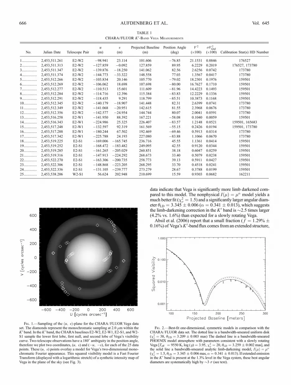
data indicate that Vega is significantly more limb darkened com-pared to this model. The nonphysical I �ð Þ ¼ �� model yields amuch better fit (�2

� ¼ 1:5) and a significantly larger angular diam-eter �LD ¼ 3:345 � 0:006 (� ¼ 0:341 � 0:013), which suggeststhe limb-darkening correction in the K 0 band is�2.5 times larger(4.2% vs. 1.6%) than expected for a slowly rotating Vega.Absil et al. (2006) report that a small fraction ( f ¼ 1:29% �

0:16%) of Vega’sK 0-band flux comes from an extended structure,

TABLE 1

CHARA/FLUOR K 0-Band Vega Measurements

No. Julian Date Telescope Pair

u

(m)

v

(m)

Projected Baseline

(m)

Position Angle

(deg)

V 2

(;100)�V 2

total

(;100) Calibration Star(s) HD Number

1................ 2,453,511.261 E2-W2 �98.941 23.114 101.606 �76.85 21.1531 0.8846 176527

2................ 2,453,511.313 E2-W2 �127.859 �0.092 127.859 89.95 6.2229 0.2019 176527, 173780

3................ 2,453,511.347 E2-W2 �139.876 �18.250 141.062 82.56 2.6256 0.0742 173780

4................ 2,453,511.374 E2-W2 �144.773 �33.322 148.558 77.03 1.3567 0.0417 173780

5................ 2,453,512.266 E2-W2 �103.834 20.146 105.770 �79.02 18.2301 0.1976 159501

6................ 2,453,512.269 E2-W2 �106.062 18.698 107.698 �80.00 16.7627 0.1710 159501

7................ 2,453,512.277 E2-W2 �110.513 15.601 111.609 �81.96 14.4223 0.1493 159501

8................ 2,453,512.284 E2-W2 �114.716 12.396 115.384 �83.83 12.2229 0.1336 159501

9................ 2,453,512.291 E2-W2 �118.435 9.291 118.799 �85.51 10.3873 0.1168 159501

10.............. 2,453,512.345 E2-W2 �140.179 �18.907 141.448 82.31 2.6399 0.0741 173780

11.............. 2,453,512.349 E2-W2 �141.068 �20.951 142.615 81.55 2.3968 0.0676 173780

12.............. 2,453,512.356 E2-W2 �142.577 �24.954 144.744 80.07 2.0041 0.0591 173780

13.............. 2,453,516.258 E2-W1 �141.950 88.392 167.221 �58.08 0.1040 0.0059 159501

14.............. 2,453,516.343 E2-W1 �224.986 25.325 226.407 �83.57 1.2148 0.0521 159501, 165683

15.............. 2,453,517.248 E2-W1 �132.597 92.319 161.569 �55.15 0.2426 0.0194 159501, 173780

16.............. 2,453,517.288 E2-W1 �180.244 67.502 192.469 �69.46 0.5913 0.0314 173780

17.............. 2,453,517.342 E2-W1 �225.788 24.193 227.080 �83.88 1.1066 0.0670 173780

18.............. 2,453,519.225 E2-S1 �169.006 �165.745 236.716 45.55 1.1361 0.0414 159501

19.............. 2,453,519.252 E2-S1 �168.472 �183.482 249.095 42.55 0.9120 0.0344 159501

20.............. 2,453,519.285 E2-S1 �161.265 �205.029 260.851 38.18 0.6047 0.0259 159501

21.............. 2,453,519.316 E2-S1 �147.913 �224.292 268.673 33.40 0.5079 0.0238 159501

22.............. 2,453,522.270 E2-S1 �163.306 �200.735 258.773 39.13 0.5911 0.0427 159501

23.............. 2,453,522.306 E2-S1 �148.868 �223.205 268.295 33.70 0.4518 0.0241 159501

24.............. 2,453,522.336 E2-S1 �131.105 �239.777 273.279 28.67 0.3788 0.0199 159501

25.............. 2,453,538.206 W2-S1 56.624 202.948 210.699 15.59 0.9303 0.0682 162211

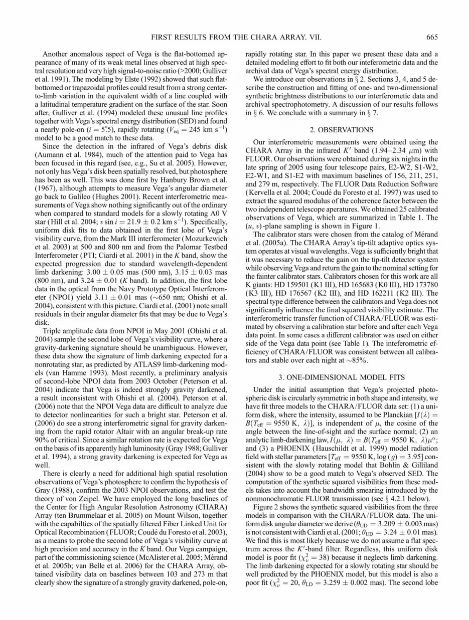
Fig. 1.—Sampling of the u; vð Þ-plane for the CHARA/FLUOR Vega dataset. The diamonds represent the monochromatic sampling at 2.0 �m within theK 0 band. In theK 0 band, the CHARAbaselines E2-W2, E2-W1, E2-S1, andW2-S1 sample the lower first lobe, first null, and second lobe of Vega’s visibilitycurve. Two-telescope observations have a 180� ambiguity in the position angle,therefore we plot two coordinates, (u; v) and (�u; �v), for each of the 25 datapoints. These (u; v) points overlay a model for Vega’s two-dimensional mono-chromatic Fourier appearance. This squared visibility model is a Fast FourierTransform (displayed with a logarithmic stretch) of a synthetic intensity map ofVega in the plane of the sky (see Fig. 3).

Fig. 2.—Best-fit one-dimensional, symmetric models in comparison with theCHARA/FLUOR data set. The dotted line is a bandwidth-smeared uniform disk(�2

� ¼ 38, �UD ¼ 3:209 � 0:003 mas) The dashed line is a bandwidth-smearedPHOENIX model atmosphere with parameters consistent with a slowly rotatingVega [TeA ¼ 9550 K, log (g) ¼ 3:95, �2

� ¼ 20, �LD ¼ 3:259 � 0:002 mas], andthe solid line a bandwidth-smeared analytic limb-darkening model, I �ð Þ ¼ ��

(�2� ¼ 1:5, �LD ¼ 3:345 � 0:006mas,� ¼ 0:341 � 0:013). If extended emission

in the K 0 band is present at the 1.3% level in the Vega system, these best angulardiameters are systematically high by �3 � (see text).

AUFDENBERG ET AL.666 Vol. 645

most likely Vega’s debris disk. In order to gauge the significanceof this extra flux on the photospheric parameters derived above,the synthetic squared visibilities are reduced by an amount equalto the square of fraction of light coming from the debris disk. Atlong baselines, the visibility of the debris disk is essentially zerosuch that

V 2obs ¼ 1� fð ÞVphotosphere þ f Vdisk

� �2 ð1Þ� 0:974V 2

photosphere:

The revised fits to V 2photosphere are �UD ¼ 3:198 � 0:003 (�2

� ¼38) for the uniform disk, �LD ¼ 3:247 � 0:002 (�2

� ¼ 19) forthe PHOENIX model, and �LD ¼ 3:329 � 0:006 (� ¼ 0:328 �0:013, �2

� ¼ 1:4) for the I �ð Þ ¼ �� model. The effect of remov-ing the extended emission is to reduce the best-fit angular diameterfor all three models by�3 �; the correction for extended emissionis therefore significant.

4. TWO-DIMENSIONAL MODEL CONSTRUCTION

In order to physically interpret the strong limb darkeningwe find for Vega, we have adapted a computer program writtenby S. Cranmer (2002, private communication) from Cranmer &Owocki (1995) that computes the effective temperature and sur-face gravity on the surface of a rotationally distorted star, spe-cifically a star with an infinitely concentrated central mass underuniform angular rotation, a Roche–von Zeipel model. This azi-muthally symmetric model is parameterized as a function of thecolatitude given the mass, polar radius, luminosity, and fractionof the angular break-up rate.

Each two-dimensional intensity map is characterized by fivevariables: �equ , the angular size of the equator, equivalent to theangular size as viewed exactly pole-on; ! ¼ �/�crit , the fractionof the critical angular break-up rate; T

poleeA , the effective temper-

ature at the pole; log gð Þpole , the effective surface gravity at thepole; and , the position angle of the pole on the sky measuredeast from north.

Given these input parameters, along with the measured trig-onometric parallax �hip ¼ 128:93 � 0:55 mas (Perryman et al.1997), and the observed projected rotation velocity, v sin i ¼21:9 � 0:2 km s�1 (Hill et al. 2004), the parameterization of theintensity maps begins with

Requ ¼ 107:48�equ�hip

; ð2Þ

with the equatorial radius in solar units and both �equ and �hip inmilliarcseconds. It follows from a Roche model (Cranmer &Owocki 1995; eq. [26]) that the corresponding polar radius is

Rpole ¼!Requ

3 cos�þcos�1 !ð Þ

3

h iand the stellar mass is

M ¼gpoleR

2pole

G; ð4Þ

where G is the universal gravitational constant. The luminosityis then

L ¼�� T

poleeA

� �4gpole

; ð5Þ

where � is the Stefan-Boltzman constant and � is the surface-weighted gravity (Cranmer & Owocki 1995; eqs. [31] and [32]),expressed as a power series expansion in !,

� � 4�GM 1:0� 0:19696!2 � 0:094292!4 þ 0:33812!6�� 1:30660!8 þ1:8286!10 � 0:92714!12Þ: ð6Þ

The ratio of the luminosity to � provides the proportionalfactor between the effective temperature and gravity for vonZeipel’s radiative law for all colatitudes # :

TeA #ð Þ ¼ L

��g #ð Þ

� �¼ T

poleeA

g #ð Þgpole

" #; ð7Þ

where the gravity darkening parameter, , takes the value 0.25in the purely radiative case (no convection). The effective tem-perature difference between the pole and equator,�TeA, may beexpressed in terms of T

poleeA and ! :

�TeA ¼ TpoleeA � T

equeA ¼ T

poleeA 1� !2

2� 8

27!

� " #; ð8Þ

where

¼ 3 cos�þ cos�1 !ð Þ

3

� �:

The effective gravity as a function of # is given by

g #ð Þ ¼ gr #ð Þ2þ g# #ð Þ2h i1=2

; ð9Þ

gr #ð Þ ¼ �GM

R #ð Þ2þ R #ð Þ � sin #ð Þ2; ð10Þ

g# #ð Þ ¼ R #ð Þ�2 sin # cos #; ð11Þ

where gr and g# are the radial and colatitudinal components ofthe gravity field. The colatitudinal dependence of the radius isgiven by

R #ð Þ ¼ 3Rpole

! sin #cos

�þ cos�1 ! sin #ð Þ3

� �! > 0ð Þ ð12Þ

and angular rotation rate is related to the critical angular rotationrate8 by

� ¼ !�crit ¼ !8

27

GM

R3pole

!1=2

: ð13Þ

At the critical rate (! ¼ 1), Requ ¼ 1:5Rpole . The inclinationfollows from

i ¼ sin�1 v sin i

Vequ

� ; ð14Þ

8 There is a typographical error in eq. (5) of Collins (1963), which is not in thepaper’s erratum (Collins 1964): !2

c ¼ GM /Re should be !2c ¼ GM /R3

e , where !c

the critical angular rate and Re is the equatorial radius at the critical rate.

FIRST RESULTS FROM THE CHARA ARRAY. VII. 667No. 1, 2006

where the equatorial velocity is

Vequ ¼ Requ�: ð15Þ

4.1. Building the Intensity Maps

For each wavelength k (185 total wavelength points: 1.9–2.4 �m in 0.005 �m steps, with additional points for H i and He iprofiles calculated in non-LTE), an intensity map is computed asfollows: TeA #ð Þ and log gð Þ#ð Þ are evaluated at 90 # points from0� to 90� þ i. At each # there are 1024 longitude ’ points from0� to 360� to finely sample the perimeter of the nearly pole-onview. For Vega’s nearly pole-on orientation, the relatively highresolution in ’ reduces numerical aliasing when the brightnessmap is later interpolated onto a uniformly gridded rectangulararray as described below.

Each set of spherical coordinates [R #ð Þ, #, ’] is first trans-formed to rectangular (x, y, z) coordinates with the InteractiveData Language (IDL) routine POLEREC3D.9 Next, the z-axis ofthe coordinate system is rotated away from the observer by anangle equal to the inclination i (using the IDL routine ROT_3D)and then the (x, y)-plane is rotated by an angle equal to , the po-sition angle (east of north) of the pole on the sky (using the IDLroutine ROTATE_XY).

At each point in the map, the cosine of the angle between theobserver’s line of sight and the local surface normal is

� x; yð Þ ¼ � #; ’; ið Þ

¼ 1

g #ð Þ

�� gr #ð Þ sin # sin i cos ’þ cos # cos ið Þ

� g# #ð Þ sin i cos ’ cos #� sin # cos ið Þ�: ð16Þ

The intensity at each point x; yð Þ is interpolated from a grid of170 spherical, hydrostatic PHOENIX (vers. 13.11.00B) stellaratmosphere models (Hauschildt et al. 1999) spanning 6500 to10,500 K in TeA and 3.25 to 4.15 in log gð Þ:

Tj ¼ 6500þ 250j K; j ¼ 0; 1; : : : ; 16f g;log glð Þ ¼ 3:25þ 0:1l; l ¼ 0; 1; : : : ; 9f g:

Four radiation fields, I k; �ð Þ evaluated at 64 angles by PHOENIX,are selected from themodel grid to bracket the local effective tem-perature and gravity values on the grid square,

Tj < TeA #ð Þ < Tjþ1;

gl < g #ð Þ < glþ1:

The intensity vectors Ik �ð Þ are linearly interpolated (in the log)at � x; yð Þ around the grid square,

I 00k ¼ Ik Tj; gl; � x; yð Þ�

;

I 10k ¼ Ik Tjþ1; gl; � x; yð Þ�

;

I11k ¼ Ik Tjþ1; glþ1; � x; yð Þ�

;

I 01k ¼ Ik Tj; glþ1; � x; yð Þ�

:

Next, the intensity is bilinearly interpolated at the local TeA andlog gð Þ for each x; yð Þ position in the map:

Ik x; yð Þ ¼ Ik TeA x; yð Þ; g x; yð Þ; � x; yð Þ½ �¼ 1� að Þ 1� bð ÞI 00k þ a 1� bð ÞI 10k

þ abI11k þ 1� að ÞbI 01k ð17Þ

where

a ¼ TeA x; yð Þ � Tj� �

= Tjþ1 � Tj�

;

b ¼ g x; yð Þ � gl½ � glþ1 � gl�

:

Finally, a Delaunay triangulation is computed (using the IDLroutine TRIGRID) to regrid the intensity map Ik x; yð Þ, originallygridded in# and’, onto a regular 512 ; 512 grid of points in x andy. The coordinates x and y have the units of milliarcseconds andcorrespond to offsets in right ascension and declination on the sky(��, �� ) relative to the origin, the subsolar point.

4.2. Synthetic Squared Visibility Computation

Due to the lack of symmetry in the synthetic intensity maps,we evaluate a set of discrete two-dimensional Fourier transformsin order to generate a set of synthetic squared visibilities com-parable to the CHARA/FLUOR observations. The first step isto compute the discrete Fourier transform for each wavelength ateach of the spatial frequency coordinates u; vð Þ correspondingto the projected baseline and orientation of each data point (seeTable 1). Themean u; vð Þ coordinates for each data point, in unitsof meters, are converted to the corresponding spatial frequencycoordinates uk ; vkð Þ in units of cycles per arcsecond for eachwavelength kk . The Fourier transform

V 2k u; vð Þ ¼

Z 1

�1

Z 1

�1SkIk x; yð Þe i2� uxþvyð Þ dx dy

� �2ð18Þ

is approximated by the integration rule of Gaussian quadrature(e.g., Stroud & Secrest 1966; Press et al. 1992):

V 2k (uk ; vk) �

XNi¼1

Ai

XNj¼1

AjSkIk(xi; yj) cos 2�(uk xiþ vk yj)� �( )2

þXNi¼1

Ai

XNj¼1

AjSkIk(xi; yj)sin 2�(uk xiþ vk yj)� �( )2

;

ð19Þ

where Sk is the wavelength discretized value of the instrumentsensitivity curve Sk, and Ai, Aj and xi, yj are the weights andnodes of the quadrature, respectively. For our square grid, thex- and y-coordinate nodes and weights are indentical. The two-dimensional Gaussian quadrature is performed with a versionof the IDL routine INT_2D modified to use an arbitrarily highnumber of nodes. The intensity at wavelength k, Ik x; yð Þ, is in-terpolated at xi; yj

� from the regular 512 ; 512 spacing to the

quadrature node points using the IDL routine INTERPOLATEwhich uses a cubic convolution interpolation method employ-ing 16 neighboring points. The synthetic squared visibility isnormalized to unity at zero spatial frequency by

V 2k 0; 0ð Þ �

XNi¼1

Ai

XNj¼1

AjSkIk xi; yj� " #2

: ð20Þ9 The coordinate transformation routines used here are from the JHU/APL /

S1R IDL library of the Space Oceanography Group of the Applied Physics Lab-oratory of Johns Hopkins University.


We find N ¼ 512 provides the degree of numerical accuracysufficient in the case of a two-dimensional uniform disk (rightcircular cylinder) to yield V 2 values in agreement with the an-alytic result,

V 2k uk ; vkð Þ ¼ 2J1 ��

ffiffiffiffiffiffiffiffiffiffiffiffiffiffiffiu2k þ v2k

q� .��

ffiffiffiffiffiffiffiffiffiffiffiffiffiffiffiu2k þ v 2k

q� � �2; ð21Þ

where J1 is the first order Bessel function of the first kind, � isthe angular diameter of the uniform disk, and B is the projectedbaseline, to better than 1% for V 2> 10�3. We use the IDL func-tion BESELJ for our J1 computations. For V 2P10�4, near themonochromatic first and second zeros, the numerical accuracyof the quadrature deteriorates to 10% or worse. The bandwidth-smeared V 2 minimum is at �10�3, so we find this quadraturemethod yields squared visibilities which are sufficiently accu-rate for our task, however observations with an even larger dy-namic range (Perrin & Ridgway 2005) will require more accuratemethods.

To test the two-dimensional Gaussian quadrature method inthe case where no analytic solution is available, we computed thetwo-dimensional fast Fourier transform (IDL routine FFT) of abrightness map (see Fig. 3). First, we compared the results of thetwo-dimensional FFT to the analytic uniform disk (eq. [21]. Toreduce aliasing we find it necessary to ‘‘zero-pad’’ the brightnessmap. With 12-to-1 zero padding (the 512 ; 512 brightness mapplaced at the center of a larger 6144 ; 6144 array of zeros), wefind the two-dimensional FFT has very similar accuracy to the512-point Gaussian quadrature: better than 1% down to V 2 k10�3 inside the second null. For the brightness map shown inFigure 3, the two-dimensional FFT and Gaussian quadraturemethods agree to better than 0.5% down to V 2k10�3, inside thesecond null. We find the computational time required to eval-uate equation (19) at 25 uk ; vkð Þ points for 185 wavelengths is�6 times faster than the evaluation of the 185 zero-padded two-dimensional FFTs.

4.2.1. Bandwidth Smearing

Once we have computed V 2k uk ; vkð Þ for the 185 wavelength

points, we proceed to compute the bandwidth-smeared averagesquared visibility V B; k0ð Þ2,

V B; k0ð Þ2 ¼R 10

V B; kð Þ2k2 dkR 10

V 0; kð Þ2k2 dk: ð22Þ

This integral is performed by the IDL routine INT_TABULATED,a five-point Newton-Cotes formula. The k2 term is included sothat the integral is equivalent to an integral over wavenumber(frequency), where

k�10 ¼

R 10

k�1S kð ÞFk dkR 10

S kð ÞFk dkð23Þ

is the mean wavenumber. This simulates the data collection andfringe processing algorithm used by FLUOR. In the discretizedintegrand V B; kkð Þ2 is equivalent to V 2

k uk ; vkð Þ, where B ¼206264:8kk u2

k þ v 2k�

1/2, with kk in units of meters and uk andvk in units of cycles per arcsecond.

4.3. Synthetic Spectral Energy Distribution Construction

To construct synthetic SEDs for Vega from the Roche–vonZeipel model, 170 radiation fields were computed from the samemodel grid used to construct the K 0-band intensity maps. The

wavelength resolution is 0.05 nm from 100 to 400 nm, 0.2 nmfrom 400 nm to 3 �m, and 10 nm from 3 to 50 �m. The higherresolution in the ultraviolet is needed to sample the strong lineblanketing in this spectral region. From the resulting grid ofradiation fields, intensity maps are computed (see x 4.1), and theflux is computed from

Fk ¼Z �

0

Z 2�

0

� g #ð Þgr #ð Þ Ik R; #; ’ð ÞR #ð Þ2 sin #� #; ’; ið Þ d’ d#:

ð24Þ

This two-dimensional integral is performed with the IDL rou-tine INT_TABULATED_2D (vers. 1.6), which first constructs aDelaunay triangulation of points in the #; ’ð Þ-plane. For eachtriangle in the convex hull (defined as the smallest convex poly-gon completely enclosing the points), the volume of the tri-angular cylinder formed by six points (the triangle in the planeand three points above with heights equal to the integrand) iscomputed and summed. For computing the flux from the inten-sity maps, a coarser sampling in # and ’ (20 ; 40), relative tothat needed for the visibility computations, is sufficient for bet-ter than 1% flux accuracy. The numerical accuracy was checkedby computing the SED of a nonrotating star (! ¼ 0) and com-paring this to a single effective temperature SED from a one-dimensional atmosphere. The interpolation and integrationerrors result in a flux deficit of less than 0.7% at all wavelengthsrelative to the one-dimensional model atmosphere.

5. TWO-DIMENSIONAL MODEL FITTING

5.1. Initial Parameter Constraints

The computation of each intensity map, the Fourier transforms,and the bandwidth-smearing for each set of input parameters [�equ,!,T pole

eA , log gð Þpole, ] is too computationally expensive to com-pute synthetic squared visibilities many hundreds of times as part

Fig. 3.—Synthetic brightness map ( linear stretch) of Vega for our best-fittingparameters: ! ¼ 0:91, �equ ¼ 3:329 mas, T

poleeA ¼ 10; 150 K, log (g)pole ¼ 4:10.

For this model, Vega’s pole is inclined 5� toward a position angle of 40�, withthe subsolar point marked with an ‘‘x.’’ The labeled intensity contours are rel-ative to the maximum intensity in the map.


of a gradient-search method over the vertices of a five-dimensionalhypercube. Therefore,wemust proceedwith targeted trial searchesto establish the sensitivity of �2

� to each parameter after first es-tablishing a reasonable range of values for each parameter.

The parameter �equ is a physical angular diameter related to auniform disk fit by a scale factor depending on the degree ofgravity and limb darkening, which in turn depends on the param-eters !, log gð Þpole , and T pole

eA , in order of importance. As shownabove, a limb-darkening correction of 4% is significantly largerthan the �1.5% value expected for a normal A0 V star at 2 �m(Davis et al. 2000). The analytic limb-darkening model fit issufficiently good that we take �equ ¼ 3:36 mas as a starting value.This corresponds to Requ ¼ 2:77 R� from equation (2).

Our starting value for ! is based on the assumption that Vega’strue luminosity should be similar to that slowly rotating A0 Vstars. Vega has an apparent luminosity, assuming a single effec-tive temperature from all viewing angles, of 57 L� based on itsbolometric flux and the parallax. In the pole-on rapidly rotatingcase, we would see Vega in its brightest projection. According toMillward &Walker (1985) the mean absolute visual magnitude,MV , is 1.0 for spectral type A0 V. With a bolometric correctionof �0.3, this translates to L ¼ 37:7 L�. From equations (5) and(6) we expect ! > 0:8 in order to account for the luminositydiscrepancy assuming a minimum polar effective temperatureof 9550 K, based on the nonrotating model fits to Vega’s SED(Bohlin & Gilliland 2004). The range of effective temperaturesand surface gravities for the model atmosphere grid described inx 4.1 sets our upper rotation limit at ! � 0:96. For ! > 0:8,�TeA > 1300 K (see eq. [8]), and thus T pole

eAmust be greater than

9550 K to compensate for the pole-to-equator temperature gra-dient and to reproduce the observed SED. So, given a mean ap-parent TeA of 9550 K, a rough estimate of T

poleeA is 9550 Kþ

12�TeA ¼ 10;200 K. We therefore limit the polar effective tem-

perature to the range 10;050 K < TpoleeA < 10;350 K.

The relationship between ! and the true luminosity, throughequations (5), (6), and (4), is independent of the polar surfacegravity; yet we can constrain log gð Þpole by assuming Vega fol-lows the mass-luminosity relation we derive for the slowly rotat-ing Sirius, L/L� ¼ M /M�ð Þ4:3�0:2

. Here we assumeVega’s rapidrotation has no significant effect on its interior in relation to theluminosity from nuclear reactions in its core. Assuming L ¼

37:7 L� from above, the mass-luminosity relation yields M ¼2:3 � 0:1 M�. As ! increases, Rpole decreases relative to Requ,therefore choosing M ¼ 2:2 M� and ! ¼ 0:8 provides a lowerlimit of log gð Þpole¼ 4:0. For lower polar gravities, Vega’s masswill be significantly lower than expected based on its luminos-ity; nevertheless, we choose a range log gð Þpole values from 3.6and 4.3 in order to check the effect of the gravity on our syn-thetic visibilities and SEDs.Finally, the position angle of Vega’s pole, , should be im-

portant if Vega’s inclination is sufficiently high and its rotationsufficiently rapid to produce an elliptical projection of the rota-tionally distorted photosphere on plane of the sky. Previousmea-surements (Ohishi et al. 2004; Ciardi et al. 2001) find no evidencefor ellipticity. Preliminary results from the NPOI three-telescopeobservations of Peterson et al. (2004) suggest an asymmetricbrightness distribution with ¼ 281�.

5.2. CHARA/FLUOR Data: Parameter Grid Search

For the grid search we compute the �2� for a set of models

defined by �equ,!, TpoleeA

, log gð Þpole , and , adjusting �equ slightly(<0.3%) to minimize �2

� for each model (see below). Figure 4shows a �2

� map in the !; ð Þ-plane for a range of �equ valueswithT pole

eA¼ 10;250K, log (g) pole ¼ 4:1.Wefind a best fit of �2

� ¼1:31 for parameters! ¼ 0:91, �equ ¼ 3:329mas, and ¼ 40

�. A

direct comparison of this model with the squared visibility data isshown in Figure 5.The F-test provides a 1 � lower limit on ! at ’0.89. For

! < 0:89, the synthetic V 2 values are generally too high acrossthe second lobe because the model is not sufficiently darkenedtoward the limb. Correspondingly, the upper limits on ! are con-strained because the synthetic V 2 values are generally too lowacross the second lobe, due to very strong darkening toward thelimb for !k 0:93. In addition, the upper limit on ! is a functionof because the projected stellar disk appears sufficiently moreelliptical, even at low inclinations i ’ 5�, as the model starrotates faster. The data from the nearly orthogonal E2-W1 andE2-S1 baselines constrain models with ! > 0:92 to limited rangeof position angles, but these data provide no constraint on atlower !-values where the star is less distorted, Requ /Rpole < 1:24.As ! increases so does the darkening of the limb due to the

increasing larger pole-to-equator effective temperature differ-ence. As a result, the best-fit �equ value increases with ! because

Fig. 4.—Contour plot of �2� in the (!; )-plane for T pole

eA ¼ 10; 250 K andlog (g)pole ¼ 4:1. The labeled contours denote the lower and upper 1� range,and a 2 � contour, from the F test. The cross marks the best fit, �2

� ¼ 1:31, whilethe brightest region has a �2

� ¼ 3:25 (see Fig. 6).

Fig. 5.—(a) CHARA/FLUOR V 2 data (error bars) plotted as a function ofprojected baseline (for a range of azimuths, see Table 1) together with the best-fitting Roche–von Zeipel synthetic squared visibilities. Model parameters:! ¼ 0:91, �equ ¼ 3:329 mas, T

poleeA ¼ 10; 250 K, log (g)pole ¼ 4:10. The best-fit

�2� ¼ 1:31. (b) Deviations of the best-fit model from observed squared visibil-

ities. The dotted and dashed lines indicated the 1 and 2 � deviations.


the effective ‘‘limb-darkening’’ correction increases. The best-fitvalues for �equ and ! are therefore correlated. To establish thiscorrelation, we estimated the best-fitting �equ value for a given !without recomputing the brightness map and Fourier compo-nents. While each intensity map is constructed for a fixed �equvalue, we can approximate the squared visibilities for modelswith slightly (<0.5%) larger or smaller �equ values as follows. Asmall adjustment to V 2 due to a small adjustment in �equ, assum-ing the physical model for the star is not significantly changedand the model changes relatively slowly with wavelength, isequivalent to computing V 2 at a larger (smaller) wavelength fora larger (smaller) value of �equ. So, for a given projected baseline,we linearly interpolate (in the log)V 2

k u; vð Þ at k ¼ kk �Bt/�equ�

, awavelength shift of 10 nm or less. Near the bandpass edges, theinstrument transmission drops to zero, so there is no concernabout interpolating outside of the wavelength grid with thisscheme. The V 2 normalization, equation (20), must be scaledby the �Bt/�equ

� 2to compensate for the revised surface area of

the star. After one iteration, setting �equ ¼ �Bt , recomputing theFourier map and refitting the data, the best-fit �equ value is within0.25% of that found with the estimated model V 2 values.

Figure 6a shows the �2� values from Figure 4 projected on the

! axis, with a spread of values for the 18 position angles at each!-value. This shows again that for the range 0:89 < ! < 0:92there is no constraint on the position angle of the pole. The cor-responding best-fit �equ values are shown in Figure 6b. The equa-torial angular diameter is constrained to the range 3:32 mas <�equ < 3:34 mas. The best fit to the CHARA/FLUOR data is in-sensitive to T

poleeA . This is because �TeA, which determines

the overall darkening, is quite sensitive to !, but T poleeA is not (see

eq. [8]). Thus, we cannot usefully constrain TpoleeA or from

the CHARA/FLUOR data. As for the surface gravity, varyinglog gð Þpole over what we consider the most probable range, 4:1 �0:1, does not significantly effect the �2

� minimum. Models withlog gð Þpole values from 3.9 to 4.3 all fall within 1 � of the best fit.The best-fit �equ values are essentially independent of T

poleeA be-

tween 9800 and 10,450 K and weakly dependent on log gð Þpole

Fig. 6.—Constraints on model parameters from the CHARA/FLUOR data. (a) Reduced �2 values �2� from the Roche-von Zeipel model fit to the squared visibility

data as a function the fraction of the critical angular break-up rate, ! ¼ �/�crit , for fixed values of the polar effective temperature TpoleeA and polar surface gravity

log gð Þpole. The dashed line denotes the 1 � confidence region for! from the F test for 24 degrees of freedom relative to the best fit at�2� ¼ 1:31. For each !,�2

� values areplotted for 18 position angles (0� to 170� in 10� steps; see Fig. 4). (b) Relationship between the best-fit equatorial angular diameter �equ at each ! for the range ofposition angles. The dashed lines provide an estimate for the 1 � range in ! and the corresponding range in the equatorial angular diameter.

Fig. 7.—Contour plot of �2� for the SED fits in the (!; T pole

eA )-plane. The !range is limited to the 1 � range from CHARA/FLUOR fits (see Fig. 6). Thepolar surface gravity is fixed at log (g)pole ¼ 4:1. The labeled contours denotethe 1 and 2 � regions from the F test. The cross marks the location of the best-fitmodel, �2

� ¼ 8:7.


between 3.8 and 4.3; all best-fit �equ values fall well within the1 � range established in Figure 6.

5.3. Spectral Energy Distribution: Parameter Grid Search

Here we compare our synthetic SEDs to the absolute spectro-photometry of Vega. Specifically, we compare our models tothe data-model composite SED10 of Bohlin & Gilliland (2004),which includes International Ultraviolet Explorer (IUE ) datafrom 125.5 to 167.5 nm, Hubble Space Telescope (HST ) SpaceTelescope Imaging Spectrograph (STIS) data from 167.5 to420 nm, and a specifically constructed Kurucz model shortwardof IUE and longward 420 nm to match and replace data cor-rupted by CCD fringing in this wavelength region. To facilitatethis comparison, first the synthetic spectra were convolved to thespectral resolution of the observations (k /�k ¼ 500), and thenboth the data and convolved synthetic spectra were binned:2.0 nm wide bins in the UV (127.5–327.5 nm, 101 bins) and2.0 nm bins in the optical and near-IR (330.0–1008 nm, 340 bins)for a total of 441 spectral bins.

Figure 7 shows the�2� map in the ð!; T pole

eA Þ-plane. These twoparameters, apart from the angular diameter, most sensitively af-fect the fit to the observed SED. There is a clear positive correlationbetween ! and T

poleeA . This makes sense if one considers that a

more rapidly rotating star will be more gravity darkened and re-quire a hotter pole to compensate for a cooler equator in order tomatch the sameSED. Following this correlation, it is expected thata continuum of models from (! ¼ 0:89, T pole

eA ¼ 10;150 K) to(! ¼ 0, T

poleeA ¼ 9550 K) will provide a reasonable fit to the SED

since the nonrotatingATLAS12model ofKurucz fits the observedSED quite well (Bohlin & Gilliland 2004). However, we did notconsider models with ! < 0:88 in the SED analysis becausesuch models are a poor match to the CHARA/FLUOR squaredvisibility data set as shown above. In other words, although theATLAS12model provides a good fit to the observed SED, it failsto predict the correct center-to-limb darkening for Vega.The best-fit synthetic spectrum is shown in Figure 8. Con-

sidering the complexity of this synthetic SED relative to a singleTeA model, there is generally good agreement (�5%) betweenour best-fit model and the data longward of 300 nm, apart fromlarger mismatches at the Paschen and Balmer edges and in theBalmer lines. Longward of 140 nm, the model agrees with theobservations to within�10%. At wavelengths below 140 nm, asmeasured by the IUE, the data are up to a factor of 2 lower thanpredicted. Our best fit yields �2

� ¼ 8:7. The overprediction be-low 140 nm has only a small effect on the synthetic integratedflux between 127.5 and 1008 nm, 2:79 ; 10�5 ergs cm�2 s�1,which is within 1.2 � of the value derived from an integration ofthe observed SED, (2:748 � 0:036) ; 10�5 ergs cm�2 s�1. Theequatorial angular diameter derived from this SED fit, �equ ¼3:407 mas, differs from the best fit to the CHARA/FLUOR data,�equ ¼ 3:329 mas, by 2.4%, a value within the uncertainty of theabsolute flux calibration.

6. DISCUSSION

The best-fit stellar parameters, based on the model fits to theCHARA/FLUOR data and archival spectrophotometry in x 5,are summarized in Table 2. As discussed in x 3, the effect of ex-tended K 0-band emission in the Vega system, if unaccounted for,is to increase the apparent angular diameter of Vega slightly,by�0.3%. Correcting for this effect via equation (1), the best-fitequatorial diameter is shifted systematically lower by 0.3% (0.01mas) to the range 3:31 mas < �equ < 3:33 mas. We find that allother parameters in Table 2 are uneffected by the extended emis-sion within the error bars given. The best-fit range for the frac-tion of the angular break-up rate, 0:89 < ! < 0:92, sensitive to

Fig. 8.—(a) Comparison between the SED of Bohlin & Gilliland (2004)and our best-fitting (�2

� ¼ 8:7) rapidly rotating SED model for Vega: ! ¼ 0:91,T

poleeA ¼ 10; 150 K, and log (g)pole ¼ 4:10. Also shown are the differences be-

tween this model and the data in (b) the region at shorter wavelengths observedby the IUE and (c) the region observed by the HST Space Telescope ImagingSpectrograph at longer wavelengths. At wavenumbers 1/k < 2:38 �m�1 the‘‘observed’’ SED is represented by a closely fitting Kurucz model spectrum (seeBohlin & Gilliland 2004).

10 At ftp://ftp.stsci.edu /cdbs/cdbs2/calspec/alpha_lyr_stis_002.fits.

TABLE 2

Fundamental Stellar Parameters for Vega

Parameter Symbol Value Reference

Fraction of the angular break-up rate........................ ! 0.91 � 0.03 CHARA/FLUOR V 2 fit

Equatorial angular diameter (mas) ............................ �equ 3.33 � 0.01 CHARA/FLUOR V 2 fit

Parallax (mas) ............................................................ �hip 128.93 � 0.55 Perryman et al. (1997)

Equatorial radius (R�) ............................................... Requ 2.78 � 0.02 Eq. (2)

Polar radius (R�)........................................................ Rpole 2.26 � 0.07 Eq. (3)

Pole-to-equator Teff difference (K) ............................ �Teff 2250þ400�300 Eq. (8)

Polar effective temperature (K)................................. TpoleeA 10,150 � 100 Fit to spectrophotometry (Bohlin & Gilliland 2004)

Luminosity (L�) ......................................................... L 37 � 3 Eq. (5)

Mass (M�).................................................................. M 2.3 � 0.2 (L/L�) = (M/M�)4.27�0.20 (from Sirius)

Polar surface gravity (cm s�2)................................... log (g)pole 4.1 � 0.1 Eq. (4)

Equatorial rotation velocity (km s�1) ....................... Vequ 270 � 15 Eqs. (13) and (15)

Projected rotation velocity (km s�1)......................... v sin i 21.9 � 0.2 Hill et al. (2004)

Inclination of rotation axis (deg)............................... i 4.7 � 0.3 Eq. (14)


the amplitude of the second lobe, is unaffected by the extendedemission because the V 2 correction is quite small there,�V 2 <0:0003, relative to the first lobe, where the correction is up to20 times larger.

One parameter that stands out is our large pole-to-equatoreffective temperature difference,�TeA ¼ 2250þ400

�300K, relative to

previous spectroscopic and spectrophotometric studies of Vega(Gulliver et al. 1994; Hill et al. 2004) for which �TeA falls intothe range 300 to 400 K. Our larger �TeA yields a much coolerequatorial effective temperature, T

equeA ¼ 7900þ500

�400 K, than mostrecently reported for Vega, 9330 K (Hill et al. 2004). The am-plitude of the second-lobe visibility measurements as observedby CHARA/FLUOR is well fit by strong darkening toward thelimb. In the context of the Roche-von Zeipel model, such dark-ening requires a large pole-to-equator TeA gradient. Consequently,we predict that Vega’s equator-on SED (that is, viewed as if i ¼90� and integrated over the visible stellar disk; see eq. [24]) has asignificantly lower color temperature and overall lower flux, par-ticularly in the midultraviolet where the flux is lower by a factorof 5, as shown in Figure 9. A debris disk, aligned with Vega’sequatorial plane as suggested by our nearly pole-on model for thestar and the recent observations of a circular disk in themid-IR (Suet al. 2005), should see a significantly less luminous, cooler SEDthan we see from the Earth. In the literature to date, modeling ofthe heating, scattering, and emission of Vega’s dusty debris diskhas assumed an irradiating SED equal to the pole-on view of Vega(see, e.g., Absil et al. 2006; Su et al. 2005). Our synthetic pho-tospheric equatorial spectrum for Vega is tabulated in Table 3. Itshould be interesting to investigate how our predicted equatorialspectrum used in such modeling will affect conclusions regardingthe amount of dust and the grain-size distribution in the debrisdisk.

Several of Vega’s fundamental stellar parameters (�TeA, Vequ, i)we derive differ significantly from those derived by Gulliveret al. (1994) and Hill et al. (2004) from high-dispersion spectros-copy. Regarding �TeA, both spectroscopic studies find ! ’ 0:5,while we find ! ¼ 0:91 � 0:03. These two !-values, along with

the corresponding TpoleeA values, 9680 and 10,150 K, in equa-

tion (8), yield �TeA values of 350 and 2250 K. The reason the!-values differ is at least partly linked to inconsistent parametersused in the spectroscopic studies. As noted in Hill et al. (2004),the Gulliver et al. (1994) study finds a low value for the polargravity, log (g)pole ¼ 3:75, which yields a mass for Vega of only1.34 M� and an inclination inconsistent with the expectedequatorial velocity. The equatorial velocity of Hill et al. (2004),Vequ ¼ 160 km s�1, is not consistent with their other param-eters [! ¼ 0:47, log (g)pole ¼ 4:0,Requ ¼ 2:73R�, i ¼ 7N9]whichshould yield instead Vequ ¼ 113 km s�1 and i ¼ 11N1. Valuesof Vequ ¼ 160 km s�1 and i ¼ 7N9 are recovered if ! ¼ 0:65,which corresponds to Vequ/Vcrit ¼ 0:47. It is possible to confuse! with Vequ/Vcrit. The two are not equivalent:

! ¼ �

�crit

Vequ

Vcrit

¼ 2 cos�þ cos�1 !ð Þ

3

� �: ð25Þ

Fig. 9.—Left: Comparison between the SED from Bohlin & Gilliland (2004; IUE and HST observations supplemented by a slowly rotating model spectrum bothbelow 127.5 nm and longward of 420 nm) and two rapidly rotating models for Vega’s SED, one viewed from an inclination of 5� (nearly pole on) and one viewed froman inclination of 90� (equator on), from an integration of two intensity maps via eq. (24) for these inclinations. Right: Comparison of the best-fit brightness distributionsfor Vega with inclinations of 5� (top) and 90� (bottom). For the equator-on view, the poles appear 10% fainter than the pole-on view due to limb darkening.

TABLE 3

A Model Equatorial Photospheric Spectral Energy Distribution

for Vega from 1020.5 8 to 40 �m (R = 500)

Wavelength

(8)(1)

Flux (Fk)a

(ergs cm�2 s�1 8�1)

(2)

1.020500000000000E+03...................................... 1.68027E+03

1.021000000000000E+03...................................... 1.65680E+03

1.021500000000000E+03...................................... 1.62296E+03

1.022000000000000E+03...................................... 1.57629E+03

1.022500000000000E+03...................................... 1.51370E+03

Note.—Table 3 is published in its entirety in the electronic edition of theAstrophysical Journal. A portion is shown here for guidance regarding itsform and content.

a The flux at a distance d from Vega in the equatorial plane is the flux fromcol. (2) multiplied by the ratio Requ /d

� 2, the ratio squared of Vega’s equatorial

radius to the distance, or 2:78/dð Þ2 when d has the units of solar radii.


For ! ¼ 0:65, the corresponding �TeA ¼ 757 K, not 350 K.Therefore, there appears to be a mismatch between the Vequ and�TeA values used in the most recent spectral analyses, and thissuggests the spectral data must be reanalyzed with a consistentmodel. A. Gulliver (2006, private communication) confirms thatHill et al. (2004) did confuse ! with Vequ/Vcrit, and this group isnow reanalyzing Vega’s high-dispersion spectrum. Our best-fitvalue for !, derived from the interferometric data, is appealingbecause, together with our derived polar effective temperature, ityields a luminosity consistent with that of slowly rotating A0 Vstars. A more slowly rotating model for Vega will have a warmerequator and an overall higher true luminosity too large for itsmass. Therefore, it seems that less rapidly rotating models forVega do not offer an explanation for the apparent overluminositywith respect to its spectral type.

Our best-fit model, while it provides self-consistent parame-ters within the Roche–von Zeipel context, has several discrep-ancies, most notably producing too much flux below 140 nmrelative to the observed SED. The limitations of the LTE metal-line blanketing for modeling Vega in the ultraviolet have recentlybeen explored byGarcıa-Gil et al. (2005). They find that in theUVthe line opacity is generally systematically too large in LTE be-cause the overionization in non-LTE is neglected. Our best modelflux below 140 nm is already too large, so a fully non-LTE treat-ment is not expected to improve this discrepancy. The Wien tailof Vega’s SED will be the most sensitive to the warmest colat-itudes near the pole. In our strictly radiative von Zeipel model,SEDswith T pole

eA < 10;050 K produce toomuch flux in the opticaland near-IR, so simply lowering T

poleeA will not solve the problem;

the temperature gradient must differ from the TeA / g0:25eA rela-tion. The equatorial effective temperature we derive, 7900 K,may indicate that Vega’s equatorial region is convective. If so,von Zeipel’s purely radiative gravity darkening exponent, ¼0:25, will not be valid near the equator. A more complex model,in which the gravity darkening transitions from purely radiativenear the pole to partially convective near the equator, may bethe next approach to take. Such a temperature profile may allowfor a cooler T

poleeA , reducing the flux discrepancy below 140 nm,

while still matching the observed optical and near-IR fluxes.Such a gradient must also improve the match to the Balmer andPaschen edges and the Balmer lines.

7. SUMMARY

We have demonstrated that a Roche–von Zeipel model atmo-sphere rotating at 91% � 3% of the angular break-up rate pro-vides a very good match toK 0-band long-baseline interferometricobservations of Vega. These observations sample the second lobeof Vega’s visibility curve and indicate a limb-darkening correction

2.5 times larger than expected for a slowly rotating A0 V star. Inthe context of the purely radiative von Zeipel gravity darkeningmodel, the second-lobe visibility measurements imply a �22%reduction in the effective temperature from pole to equator. Themodel predicts an equatorial velocity of 270 � 15 km s�1, whichtogether with the measured v sin i yields an inclination of i ’ 5�,confirming the pole-on model for Vega suggested by Gray (1988)to explainVega’s anomalous luminosity. Ourmodel predicts a trueluminosity for Vega of 37 � 3 L�, consistent with the mean lu-minosity of A0 V stars fromW H�ð Þ-MV calibration (Millward &Walker 1985). We predict that Vega’s spectral energy distribu-tion viewed from its equatorial plane is significantly cooler thanviewed from its pole. This equatorial spectrum may significantlyimpact conclusions derived from models for Vega’s debris diskthat have employed Vega’s observed polar-view spectral energydistribution, rather than the equatorial one, which seems moreappropriate given our observations.

We thank G. Romano and P.J. Goldfinger for their assis-tance with the operation of FLUOR and CHARA respectively.F. Schwab kindly provided advice on two-dimensional FFTsand aliasing. Thanks to T. Barman for discussions about nu-merical cubature and to the entire PHOENIX development teamfor their support and interest in this work. Thanks to refereeA. Gulliver for his careful reading and suggestions. This workwas performed in part under contract with the Jet PropulsionLaboratory (JPL), funded by NASA through theMichelson Fel-lowship Program. JPL is managed for NASA by the CaliforniaInstitute of Technology. The National Optical Astronomy Ob-servatory is operated by the Association of Universities for Re-search in Astronomy (AURA), Inc., under cooperative agreementwith the National Science Foundation (NSF). This research hasbeen supported byNSFgrantsAST 02-05297 andAST 03-07562.Additional support has been received from the Research ProgramEnhancement program administered by the Vice-President forResearch at Georgia State University. In addition, the CHARAArray is operated with support from the Keck Foundation andthe Packard Foundation. This research has made use of NASA’sAstrophysics Data System, and the SIMBAD database, operatedat CDS, Strasbourg, France. Some of the data presented in thispaper was obtained from the Multimission Archive (MAST) atthe Space Telescope Science Institute (STScI). STScI is operatedby AURA, Inc., under NASA contract NAS5-26555. Supportfor MAST for non-HST data is provided by the NASA Office ofSpace Science via grant NAG5-7584 and by other grants andcontracts.

Facilities: CHARA (FLUOR)

REFERENCES

Absil, O., et al. 2006, A&A, 452, 237Aumann, H. H., et al. 1984, ApJ, 278, L23Bohlin, R. C., & Gilliland, R. L. 2004, AJ, 127, 3508Ciardi, D. R., van Belle, G. T., Akeson, R. L., Thompson, R. R., Lada, E. A., &Howell, S. B. 2001, ApJ, 559, 1147

Collins, G. W. 1963, ApJ, 138, 1134———. 1964, ApJ, 139, 1401———. 1966, ApJ, 146, 914Collins, G. W., & Sonneborn, G. H. 1977, ApJS, 34, 41Coude du Foresto, V., Ridgway, S., & Mariotti, J.-M. 1997, A&AS, 121, 379Coude du Foresto, V., et al. 2003, Proc. SPIE, 4838, 280Cranmer, S. R., & Owocki, S. P. 1995, ApJ, 440, 308Davis, J., Tango, W. J., & Booth, A. J. 2000, MNRAS, 318, 387Elste, G. H. 1992, ApJ, 384, 284Garcıa-Gil, A., Garcıa Lopez, R. J., Allende Prieto, C., & Hubeny, I. 2005, ApJ,623, 460

Gray, R. O. 1985, JRASC, 79, 237———. 1988, JRASC, 82, 336Gulliver, A. F., Adelman, S. J., Cowley, C. R., & Fletcher, J. M. 1991, ApJ,380, 223

Gulliver, A. F., Hill, G., & Adelman, S. J. 1994, ApJ, 429, L81Hanbury Brown, R., Davis, J., Allen, L. R., & Rome, J. M. 1967, MNRAS,137, 393

Hardorp, J., & Strittmatter, P. A. 1968, ApJ, 151, 1057Hauschildt, P. H., Allard, F., Ferguson, J., Baron, E., & Alexander, D. R. 1999,ApJ, 525, 871

Hearnshaw, J. B. 1996, The Measurement of Starlight: Two Centuries of As-tronomical Photometry (Cambridge: Cambridge Univ. Press)

Hill, G., Gulliver, A. F., & Adelman, S. J. 2004, in IAU Symp. 224, The A-StarPuzzle, ed. J. Zverko, J. Ziznovsky, S. J. Adelman, & W. W. Weiss (Cam-bridge: Cambridge Univ. Press), 35

Hughes, D. W. 2001, J. British Astron. Assoc., 111, 266


Kervella, P., Segransan, D., & Coude du Foresto, V. 2004, A&A, 425, 1161Kervella, P., Thevenin, F., Morel, P., Borde, P., & Di Folco, E. 2003, A&A,408, 681

Maeder, A., & Peytremann, E. 1970, A&A, 7, 120McAlister, H. A. 1985, in IAU Symp. 111, Calibration of Fundamental StellarQuantities, ed. D. S. Hayes & A. G. D. Philip (Dordrecht: Reidel), 97

McAlister, H. A., et al. 2005, ApJ, 628, 439Merand, A., Borde, P., & Coude du Foresto, V. 2005a, A&A, 433, 1155Merand, A., et al. 2005b, A&A, 438, L9Millward, C. G., & Walker, G. A. H. 1985, ApJS, 57, 63Mozurkewich, D., et al. 2003, AJ, 126, 2502Ohishi, N., Nordgren, T. E., & Hutter, D. J. 2004, ApJ, 612, 463Perrin, G., & Ridgway, S. T. 2005, ApJ, 626, 1138Perryman, M. A. C., et al. 1997, A&A, 323, L49

Peterson, D. M., et al. 2004, Proc. SPIE, 5491, 65———. 2006, ApJ, 636, 1087Petrie, R. M. 1964, Publ. Dom. Astrophys. Obs. Victoria, 12, 317Press, W. H., Teukolsky, S. A., Vetterling, W. T., & Flannery, B. P., ed. 1992,Numerical Recipes in FORTRAN (2nd ed.; Cambridge: Cambridge Univ.Press)

Stroud, A. H., & Secrest, D. 1966, Gaussian Quadrature Formulas (EnglewoodCliffs: Practice Hall)

Su, K. Y. L., et al. 2005, ApJ, 628, 487ten Brummelaar, T. A., et al. 2005, ApJ, 628, 453van Belle, G. T., et al. 2006, ApJ, 637, 494van Hamme, W. 1993, AJ, 106, 2096von Zeipel, H. 1924a, MNRAS, 84, 665———. 1924b, MNRAS, 84, 684

Note added in proof.—New closure phase operations of Vega at visual wavelenghts with the Navy Prototype Optical Interfer-ometer (D. M. Peterson et al., Nature, 440, 896 [2006]) are also consistent with a rapidly rotating model for Vega. The Peterson et al.model establishes values for Vega’s mass, equatorial velocity, polar surface gravity, inclination, angular velocity, polar radius, andequatorial effective temperature that overlap with our values within the uncertainties. While both the Peterson et al. model and ourmodel appear to have the same Roche-von Zeipel formalism, the two data sets andmodels yield significantly different equatorial radii:Requ ¼ 2:78 � 0:02 R� (CHARA/FLUOR) versus 2:873 � 0:026 R� (NPOI). This difference is directly linked to a difference in thederived angular size of Vega’s equator in two studies: �equ ¼ 3:33 � 0:01 mas (CHARA/FLUOR) versus 3:446 � 0:031 mas(NPOI). We do not at present understand the reason for this dependency.


ERRATUM: ‘‘FIRST RESULTS FROM THE CHARA ARRAY. VII. LONG-BASELINE INTERFEROMETRICMEASUREMENTS OF VEGA CONSISTENT WITH A POLE-ON, RAPIDLY ROTATING STAR’’

(ApJ, 645, 664 [2006])

J. P. Aufdenberg, A. Merand, V. Coude du Foresto, O. Absil, E. Di Folco, P. Kervella, S. T. Ridgway,

D. H. Berger, T. A. ten Brummelaar, H. A. McAlister, J. Sturmann, L. Sturmann, and N. H. Turner

Because of an error in entering proof corrections, the term log ((g)#) in x 4.1 should read log (g(#)). In addition, equation (25) ismissing a ‘‘not equivalent’’ symbol and should read:

! ¼ �

�crit

6� Vequ

Vcrit

¼ 2 cos

��þ cos�1(!)

3

�: ð25Þ

The Press sincerely regrets these errors.

The Astrophysical Journal, 651:617, 2006 November 1

# 2006. The American Astronomical Society. All rights reserved. Printed in U.S.A.

617

Documents

First Results from the CHARA Array. VII. Long‐Baseline Interferometric Measurements of Vega Consistent with a Pole‐On, Rapidly Rotating Star