Embed Size (px)
Citation preview
FISCAL FORECAST ERRORS: GOVERNMENTS VS INDEPENDENTAGENCIES?
Rossana Merola and Javier J. Pérez
Documentos de Trabajo N.º 1233
2012

FISCAL FORECAST ERRORS: GOVERNMENTS
VS INDEPENDENT AGENCIES?
(*) The views expressed in this paper are the authors’ and do not necessarily reflect those of the Banco de España, the Eurosystem or the OECD. Merola contributed to this paper mainly while she was a European Central Bank staff member. We thank Marta Botella and Laura Fernández-Caballero for excellent research assistance. We also thank participants at the International Symposium on Forecasting (San Diego), the ESCB-Working Group on Public Finance meeting (Cyprus), the Banco de España seminar, the CESiFO Workshop on Political Economy (Dresden), the European Commission, the Workshop on International Economics (Granada) and the Economod2012 Conference (Seville), in particular Michael Berlemann, Enrique Moral, Lucio Pench, Jan-Christoph Rülke, and Ernesto Villanueva, for helpful comments. Correspondence to: Javier J. Pérez ([email protected]), Servicio de Estudios, Banco de España, c/ Alcalá 48, 28014 Madrid, Spain.
Documentos de Trabajo. N.º 1233
2012
Rossana Merola
OECD
Javier J. Pérez
BANCO DE ESPAÑA
FISCAL FORECAST ERRORS: GOVERNMENTS
VS INDEPENDENT AGENCIES? (*)
The Working Paper Series seeks to disseminate original research in economics and fi nance. All papers have been anonymously refereed. By publishing these papers, the Banco de España aims to contribute to economic analysis and, in particular, to knowledge of the Spanish economy and its international environment.
The opinions and analyses in the Working Paper Series are the responsibility of the authors and, therefore, do not necessarily coincide with those of the Banco de España or the Eurosystem.
The Banco de España disseminates its main reports and most of its publications via the INTERNET at the following website: http://www.bde.es.
Reproduction for educational and non-commercial purposes is permitted provided that the source is acknowledged.
© BANCO DE ESPAÑA, Madrid, 2012
ISSN: 1579-8666 (on line)
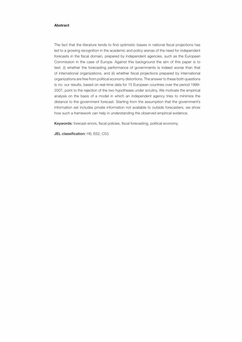
Abstract
The fact that the literature tends to fi nd optimistic biases in national fi scal projections has
led to a growing recognition in the academic and policy arenas of the need for independent
forecasts in the fi scal domain, prepared by independent agencies, such as the European
Commission in the case of Europe. Against this background the aim of this paper is to
test: (i) whether the forecasting performance of governments is indeed worse than that
of international organizations, and (ii) whether fi scal projections prepared by international
organizations are free from political economy distortions. The answer to these both questions
is no: our results, based on real-time data for 15 European countries over the period 1999-
2007, point to the rejection of the two hypotheses under scrutiny. We motivate the empirical
analysis on the basis of a model in which an independent agency tries to minimize the
distance to the government forecast. Starting from the assumption that the government’s
information set includes private information not available to outside forecasters, we show
how such a framework can help in understanding the observed empirical evidence.
Keywords: forecast errors, fi scal policies, fi scal forecasting, political economy.
JEL classifi cation: H6, E62, C53.
Resumen
Las previsiones presupuestarias que preparan las autoridades nacionales tienden a
presentar, en promedio, una visión optimista de la senda futura de las fi nanzas públicas.
Este hecho ha sido probado en numerosos trabajos; en particular, en el caso de Europa,
en la última década. Por ello, se escuchan voces que piden que otras instituciones,
independientes de los Gobiernos nacionales, asuman un papel más relevante en el proceso
de planifi cación presupuestaria. En particular, en el caso de Europa, se menciona a la
Comisión Europea. En este marco, el objetivo del presente documento es contrastar dos
cuestiones muy concretas con respecto a las previsiones presupuestarias preparadas por las
instituciones internacionales: i) ¿es la exactitud de dichas proyecciones mucho mejor que la
de las preparadas por las autoridades nacionales?, y ii) ¿están libres dichas previsiones de
distorsiones derivadas de factores tales como los ciclos electorales? Nuestros resultados,
basados en una muestra de datos (previsiones) obtenidos de informes publicados en tiempo
real para 15 países europeos en el período 1999-2007, señalan que la respuesta a las dos
preguntas es negativa. Además de la evidencia empírica, en el documento se desarrolla
un modelo teórico muy estilizado con el que se proporciona una posible explicación de los
resultados empíricos. Dicha explicación se basa en la idea de que las autoridades nacionales
disponen de más información que los analistas externos en todas las etapas de elaboración y
seguimiento de los planes presupuestarios. Así pues, la institución independiente, al tratar
de aproximarse lo más posible a la previsión del Gobierno (para reducir el défi cit de acceso
a la información), puede acabar incorporando en su propia previsión parte del sesgo político
habitual en las proyecciones ofi ciales.
Palabras clave: errores de previsión, política fi scal, predicción presupuestaria, economía
política.
Códigos JEL: H6, E62, C53.
BANCO DE ESPAÑA 7 DOCUMENTO DE TRABAJO N.º 1233
1 Introduction
Should the role of preparing budgetary projections be delegated to an independent agency?
This debate has been recently spurred in Europe by many voices, given the high public
deficit and debt levels currently held by many European Union (EU) countries. In fact,
planned government deficits turned out to exceed recurrently budgetary plans by a significant
magnitude in recent years. For example, as late as October 2008 the public deficits estimated
for 2008 by many European governments missed by some 2 percentage points of GDP the
afterwards released figures for 2008. A similar situation occurred in 2009, 2010 and 2011,
leading many countries to register record high government deficits. Explanatory factors for
this misalignments include large GDP shocks and fiscal stimulus packages adopted on the run,
but beyond this, also lack of both transparency and a realistic account of facts. As short-run
budgetary targets were missed by far, medium run plans were revised quickly and resulted
in a fast decline of the credibility of Europe’s fiscal framework, namely the Stability and
Growth Pact (SGP). As a consequence, right now, many European countries are embarking
in widespread medium-term fiscal consolidation packages, that require adherence to strict
budgetary targets for long periods of time. In parallel, there is an ongoing policy debate on
the need to strengthen economic governance in the EU that has already been materialized
in a number of reform proposals.1
The recent deterioration of public deficits and the lack of accuracy of fiscal projections
are not issues confined to the current juncture or only to EU countries’ governments. Indeed,
a great deal of the literature has analyzed in the recent past the potential bias the political
and institutional process might have on government revenue and spending forecasts,2 and
the nature and properties of forecast errors within national states.3 For the case of EU
governments, this literature tends to find evidence in favor of the existence of systematic po-
1On the importance of the design of fiscal rules and forms of governance in EU countries seeHallerberg et al. (2007). For the discussion on EU’s fiscal framework weaknesses and needs for re-form see, for example, Larch, van den Noord and Jonung (2010). For the most recent approvedand ongoing reforms and/or agreements, see EC’s webpage dedicated to EU economic governance(“http://ec.europa.eu/economy finance/economic governance/index en.htm”).
2See for example Bruck and Stephan (2006), Jonung and Larch (2006), Pina and Venes (2011), Boylan(2008), Beetsma et al. (2009), or von Hagen (2010), and the references quoted therein.
3See the survey in or Leat et al. (2008), or Frankel (2011) for a recent contribution.
BANCO DE ESPAÑA 8 DOCUMENTO DE TRABAJO N.º 1233
litical and institutional biases in revenue forecasting, while the evidence for the US is mixed,
depending on the institutional coverage of the analysis (Federal government or States).4
One particular aspect under evaluation in the policy fora linked to the previous discussion
is the proposal to introduce independent forecasts in the fiscal domain (Debrun et al. 2009;
Leeper 2009; Wyplosz 2008; Jonung and Larch 2006; European Commission 2006) prepared
by independent agencies. These independent agencies could be for example national councils
or intergovernmental agencies. As regards the latter option, in the case of EU countries, some
authors have advocated that the European Commission (EC) should have some role as the
“independent agency” preparing budgetary and/or macroeconomic projections, given that
fiscal forecasts by national authorities are scrutinized by the EC in application of EU’s fiscal
rules framework (the SGP)5.
Against this framework, in order to be in a position to judge the appropriateness of such
proposals, the relevant question to answer would be: has the track record of international
agencies’ forecasts been better than the one of national governments? In this particular
respect the literature is almost silent. There are almost no studies that compare the accu-
racy of government forecasts and fiscal forecast error’s determinants with those produced by
international organizations for a given country. The fact that some international organiza-
tions like the EC, the OECD or the IMF do publish fiscal forecasts and have been doing so
for long periods of time provides a natural laboratory to analyze their track record against
that of national governments. From a theoretical point of view, once accounting for errors
in macroeconomic forecasts, independent agencies’ fiscal forecasts should not be expected
to display the biases typically found in government’s fiscal projections. Nevertheless, one
may also claim that information matters when preparing budgetary projections, and as a
4As Auerbach (1999) argues, if the costs of forecast errors were symmetric (i.e. if positive errors were asbad as negative errors), the forecasts should present no systematic bias (i.e. on average the forecast errorshould not differ significantly from zero). There are, however, reasons to presume that the loss function ofgovernments may not be symmetric. Thus a kind of bias in fiscal forecasts could be optimal. For instance,a government would tend to favor a deficit when the loss of an underestimation is greater (for example,a conservative, stability oriented government, see Bretschneider et al. 1989). Public authorities may havean interest in presenting a pessimistic forecast to build in a safety margin that would allow them to meetbudgetary targets, also in case of revenue or expenditure slippages. The literature in question finds mixedevidence for political economy-based explanations of this sort. See Leal et al. (2008) for a broad survey ofthe issues discussed here.
5See for example Buti and van den Noord (2004).
BANCO DE ESPAÑA 9 DOCUMENTO DE TRABAJO N.º 1233
consequence outside forecasts (from independent organizations) could turn out to be less
accurate than inside forecasts (from staff of the relevant organizations, like for example the
Ministry of Finance or the Treasury), as found by Grizzle and Klay (1994) for the US states.
In our paper we provide homogeneous and comprehensive empirical evidence pointing to
the fact that international agencies’ track record of budgetary forecasts for EU countries do
present bias and correlation with electoral cycles. To unveil those results, we use a common
methodology (same econometric method, same empirical specification) to look at alternative
datasets, over the same sample period. We build up a large real-time dataset covering fiscal
forecasts: (i) that are prepared by national governments (GOV), the EC and the OECD;
(ii) for 15 European countries; (iii) for two forecast origins per year, spring and autumn
of each year; (iv) for two forecast horizons (current year and one year ahead). We focus
on the sample 1999-2007 to eliminate three potential sources of distortions: (i) the changes
in statistical standards that did occur in the preceding period (ESA79-ESA95 changeover);
(ii) the EMU convergence process; (iii) the great recession that started in 2008. Thus, we
analyze a period with a common monetary policy regime (Eurosystem), and a common fiscal
policy regime (SGP).
We try to illustrate the empirical analysis in the framework of a model in which the
independent (international) agency tries to minimize the distance to government forecasts.
We exploit the idea that government’s information set includes private information (better
access to the relevant data, information on policy measures, etc) not available to outside
forecasters (like the EC). When preparing their fiscal projections, EC staff tries to grasp
as much private information as possible from government’s, while at the same time face
a “signal extraction problem” when trying to disentangle “political biases” from genuine
“private information”.
The rest of the paper is organized as follows. In Section 2 we present some political
economy arguments to frame the subsequent empirical analysis, pose the hypotheses to
be tested, and discuss the related literature. Then, in Section 3, we describe the data
and variables used in the empirical analysis. This is done in Section 4, where we discuss
the empirical methodology and the main results. Finally, in Section 5 we present some
conclusions.
BANCO DE ESPAÑA 10 DOCUMENTO DE TRABAJO N.º 1233
2 Some political economy considerations
2.1 Political economy arguments and literature review
Why could fiscal forecasts prepared by governmental agencies differ from those of inter-
national organizations? First, fiscal forecasts can display differences because governments
usually have access to more information than outside forecasters. For example, govern-
ments have advanced information on short-term tax developments, the design and impact of
planned tax measures or information on the implementation of spending plans. Indeed, in
many cases some levels of government for which few published short-term fiscal information
is available to outsiders within a reasonable time lag, like regional and local governments,
do account for a substantial share of general government spending.
Second, the methods used by government officials and independent agencies’ Staff for
revenue and spending estimation and forecasting, can be different. Government forecasts
are prepared for all budgetary items and thus the approach typically followed is a bottom-
up one, with an extremely high level of disaggregation, while fiscal forecasts by international
organizations are prepared for fewer, more aggregated budgetary items (see Leal et al. 2008).
At the same time, it is typically the case that the forecasting methods used by international
agencies to forecast those more aggregated items tend to be more sophisticated.
Third, governments can influence forecasts prepared by international organizations, as
national countries are shareholders of these organizations and thus have the possibility to
know those forecasts in advance and discuss them with the Staff of the relevant organization;
for example, IMF Article IV reports (country reviews) acknowledge the discussions with
government officials and signal discrepancies in assessment.6
Finally, given the latter point, the fact that governments do have access to private infor-
mation, and given also that international organizations tend to be shorter of specialized Staff
than national organizations, intergovernmental agencies’ reports usually have to broadly ex-
plain the reasons for any departure from national government’s forecasts. Along these lines,
6Artis and Marcellino (2001) argue that the OECD is freer from the political pressures of EU governmentsthan the EC. Poplawski-Ribeiro and Rulke (2010), though, do not find the data supporting the latterhypothesis. Christodoulakis and Mamatzakis (2009) note that even though year-ahead government balanceforecasts are symmetric for most EU-15 countries, there seemed to be some leeway against breaching the 3%threshold value, especially for higher debt countries.
BANCO DE ESPAÑA 11 DOCUMENTO DE TRABAJO N.º 1233
one could also argue that international organizations do not have the resources to make
their own forecasts for each individual member state and, therefore, must rely heavily on the
information conveyed to them by the member states.7
The evidence on the track record of international organizations as regards fiscal pro-
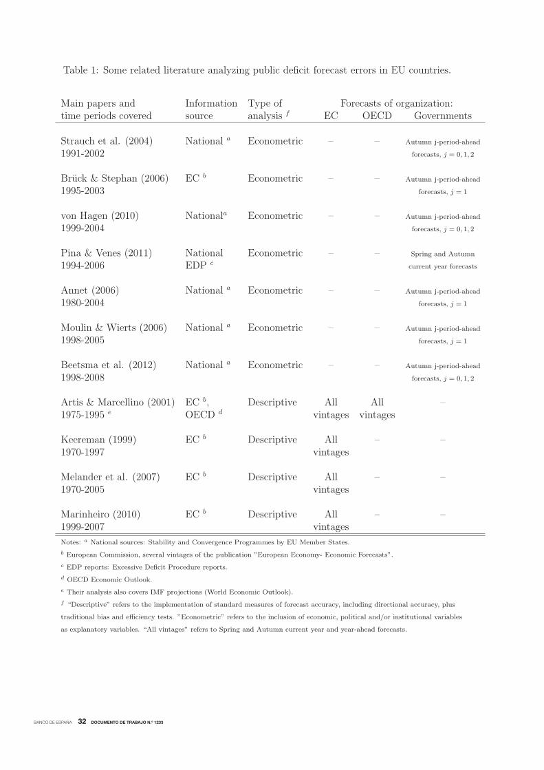
jections is scarce, and mainly descriptive.8 This should be clear when inspecting Table 1,
where we list the main papers dealing with the analysis of government balance’s forecast
errors in Europe. Most papers analyze budgetary forecasts prepared by the governments
and typically try to explain fiscal forecast errors (or only forecasts) by means of explana-
tory variables labeled as economic (like actual/forecast GDP growth or the output gap) and
political/institutional (like election year or fiscal governance structure). These papers typ-
ically focus on one vintage of projections.9 The papers that analyze projections prepared
by international organizations tend to look at the properties of the whole vintage of fore-
casts errors10 but following a descriptive approach (i.e. size and sign of errors, presence of
biases, rationality), and do not provide comparisons with budgetary forecasts prepared by
the national governments.
2.2 A stylized model to frame the discussion
With all these considerations in mind, it is fair to conceive the preparation of fiscal forecasts
by independent agencies, from a conceptual point of view, as an exercise that tries to min-
imize a certain loss function of the distance to government’s projections. Auerbach (1999)
develops a model for a different problem than ours, whose main elements can be adapted
in such a way that it is suitable for the discussion of the issues at hand here. Let Ω be the
information set commonly observed by all fiscal forecasters, be them government officials or
7This argument is taken from von Hagen (2010), that applies it to fiscal forecasts prepared by theEuropean Commission.
8As regards their GDP and inflation forecasts track records, these seem to have been reasonable in termsof size and directional accuracy, as can be inferred from Marinheiro (2010), Dreher et al. (2008), Melenderet al. (2007), Aldenhoff (2007), Timmermann (2007), Artis and Marcellino (1998, 2001), Pons (2000) orKeereman (1999). Nevertheless, some works point to a worse accuracy record than that of private sectoranalysts (see Batchelor, 2001, Blix et al., 2001, or Poplawski-Ribeiro and Rulke, 2010). Also, Aldenhoff(2007) reveals significant correlation with election dates in the case of IMF GDP forecasts for the US.
9By a vintage of projection we mean a forecast prepared at a given point in time for a given forecasthorizon like, for example, forecasts published in Autumn of year t for year t+1.
10Typically forecasts are published in Spring and Autumn of each year and provide projections for thecurrent year, one year ahead and, in some cases, two- and three years ahead.
BANCO DE ESPAÑA 12 DOCUMENTO DE TRABAJO N.º 1233
international agencies’ Staff. Let x be the variable to be forecast, say government budget
balance, revenue or expenditure. Then, the best prediction that could be done on the basis
of Ω using a commonly understood forecast methodology would be:
xΩ = E (x|Ω) (1)
where E (x|Ω) denotes the conditional expectation of x given the information set Ω.
Now, let Π be the information set comprising some private information known only by the
government, where Ω ⊂ Π. The best forecast prepared by the government would then be:
xΠ = E (x|Π) (2)
while the associated forecast error would be x− xΠ = ε, where ε is a stochastic, possibly
zero mean, error. If Π were the true information set, ε would have zero mean. Given that the
international agency (call it EC) only has partial access to government’s private information,
its forecast error would be such that x− xΩ = ν+ε, where ν is orthogonal to ε and it denotes
the additional error that the EC would commit because of its lack of access to government’s
private information set.11
The government has two options. First, it can prepare the best possible forecast given
its information set, xΠ, as in (2), in which case it would minimize a loss function of the
sort Λ1 = E[xΠ− x|Π]2. Nevertheless, as signalled by the literature on politically-motivated
fiscal forecast biases, the government has a second option. It can aim at minimizing a loss
function of this sort: Λ2 = E[(xΠ − x− θ)|Π]2, where θ is a bias included in the forecasting
process for political reasons. In this case, the best (constrained) forecast prepared by the
government would be xθΠ = xΠ + θ so that the associated forecast error would be:
x− xθΠ = ε+ θ (3)
where θ is a negative parameter if x does refer to the government balance.
The independent agency, in turn, has also two options. First, it can prepare a fully
independent forecast that can be compared ex-post with government’s forecast. In this case,
11Under the assumption that the technical forecast error ε is the same for the two institutions. In practice,two different ε-type error could be considered, due to differences in forecasting methods. This is immaterialfor the discussion at hand and thus it is left aside at this point.
BANCO DE ESPAÑA 13 DOCUMENTO DE TRABAJO N.º 1233
though, the independent agency would loose any access to government’s private information.
Then, the second option would be to try to minimize the distance to the forecast of the
government, so that the error term ν is minimized; in actual situations, the second alternative
tends to be the preferred one, not only because of the existence of private information on
the side of governments, but also due to institutional and policy constraints, as discussed
above. Thus, in this latter case the independent agency when minimizing its loss function
(distance to government’s forecast) knows that its forecast error would be:
x− xΩ = ν + θ + ε (4)
and as a consequence knows that it has to disentangle the contribution of each of the three
components of the error term: (i) ε, the technical error (model error); (ii) θ, the political–
bias–induced error; (iii) ν, the part of the overall error due to access to limited information.
Thus, the cost for the EC of trying grasp as much private information as possible – aiming
at reducing the term ν – is that it will inherit to some extent government’s political–bias, θ.
In the latter respect, one particular device to ex-ante reduce the size of θ would be the
following. Suppose that the EC were in a position to impose sanctions on the government
depending on how far their fiscal forecasts had been from the final outcome. In this case, it
could influence the extent to which the government bases its forecast on Ω rather that Π.
This can be done by imposing a penalty on the government if it deviates from a forecast
based on the common information set, xΩ. This idea is developed in Appendix A, where we
show how the EC could choose the value of the relative penalty that minimizes its expected
loss function in order to force the government to use its superior information. In general,
nonetheless, the EC will try to minimize the distance to biased government projections, by
minimizing a loss function of the kind LEC = E[(x − {xΠ + θ})| Ω]2. Thus, the EC knows
that it will incur in an error given by (4).
In order to separate, ex-post, the different sources of error, the EC has to form beliefs
about θ, ν, and ε. In this respect, the EC knows that, in general, (x− xΩ) would be a
function of the errors, call it Φ(θ, ν, ε). In order to isolate ν (good) from θ (bad) from ε
(technical) it has to form a belief on the form of Φ(θ, ν, ε). For example, Φ(θ, ν, ε) can adopt
the form of a linear projection on a constant and a function of some of the likely fundamentals
BANCO DE ESPAÑA 14 DOCUMENTO DE TRABAJO N.º 1233
of the political bias, like Φ(θ, ν, ε) ≈ c(ν, θ)+Θ(s, ELEC)+ ξ, where s is a variable linked to
the state of the business cycle and ELEC a variable that captures the electoral cycle, and ξ
is a normally distributed zero-mean random disturbance term. The constant c would proxy
the systematic part of the information bias, but also part of the political bias,12 while the
function Θ(s, ELEC) would proxy the part of the political bias determined by fundamentals.
From the empirical point of view the EC could run a standard linear regression on the series
of its forecast errors (as it is customary in the extant literature):
x− xΩ = δ0 + δ1 ELEC + δ2 s+ ξ (5)
where time subindexes have been dropped for simplicity and s could be proxied by the
forecast errors committed by the EC when forecasting real GDP. In this way, it will get
estimates of the coefficients in the regression: δ0, δ1 and δ3. Even if the constant, δ0, can
be partly interpreted as reflecting the lack-of-access-to-the-private-information-bias, it will
also reflect part of the political bias if we assume that the EC is minimizing the distance
to government’s projections; if EC forecasts were produced independently, the constant
would just capture the first factor. Now, it is feasible within our framework that δ1 turns
out to be statistically different from zero, given that it would capture also part of the
”inherited” political bias. In fact, even though δ2 should capture the genuine impact of
errors in forecasting GDP on fiscal forecast errors (most notably in revenue estimation), it
could also be the case that it is affected by political biases, to the extent that political cycles
are linked to the state of the business cycle.
A similar regression of the type of (5) run on government’s projection errors would pro-
duce a set of coefficients, δGOV0 , δGOV
1 and δGOV2 , that can be compared with δ0, δ1 and δ2.
The difference of constant terms δ0 − δGOV0 would be difficult to interpret, as it will mix-up
all the sources of bias discussed above, even though the coefficient for the government would
have a clean interpretation as political bias, as it is usually interpreted in the literature. As
regards δ1 − δGOV1 , one might expect it to be negative as assumedly EC projections should
only be affected by political cycles in an indirect way, i.e. through government projections, as
discussed above. Finally, as to δ2− δGOV2 , the expected sign would be positive as government
12It could also be the case that ε had non-zero mean, associated to non-optimal forecasts’ productionprocesses and the use of non-optimal forecasting methods, in which case the constant would also partiallyreflect this.
BANCO DE ESPAÑA 15 DOCUMENTO DE TRABAJO N.º 1233
projections tend to be more judgemental than the ones of international organizations, beign
thus less sensitive to changes in macro fundamentals.
2.3 Hypotheses to be tested
The theoretical discussion in the previous subsections do have implications for the empirical
part that follows and constitutes the main body of our paper, in particular as regards the
interpretation of the results. Against the previous discussion, we are interested in testing
the following hypotheses:
H1: The forecast performance of governments as regards budgetary projections is worse
than that of international organizations (like the EC and the OECD).
H2: Fiscal projections prepared by international organizations are not subject to political
economy distortions.
Given the stated political economy arguments, ex-ante it is far from obvious what to
expect from the empirical results. On the one hand, one may expect that neither H1 not
H2 are rejected, given the vast available empirical literature on politically-motivated fiscal
projections by governments and under the assumption that international organizations pre-
pare truly independent forecasts. On the other hand, though, if international organizations
were to face some type of “signal extraction problem” of the kind discussed above, one may
expect that both H1 and H2 are rejected.
In the subsequent sections we will aim at shedding some light on these issues. Quite
importantly, it has to be mentioned up-front that to answer these questions we use a common
methodology, i.e. the same econometric method and the same empirical specification, to look
at several alternative datasets (by institution, by vintage), over the same sample period.
3 Data description
3.1 The real-time database of fiscal forecast errors
Let us denote by dt+1 the government balance observed in year t+1. International agencies
typically prepare forecasts for dt+1 at different moments in time within a year. In order
to maximize the number of available observations, we take in our paper the sequence of
projections of dt+1 that starts with a projection prepared with information up to Spring
BANCO DE ESPAÑA 16 DOCUMENTO DE TRABAJO N.º 1233
of year t (Spring one-year-ahead forecast), and then it is updated in Autumn of year t
(Autumn one-year-ahead forecast), and further in year t + 1 in Spring (Spring current-
year forecast) and Autumn (Autumn current-year forecast). Notice that the four described
forecasts for dt+1 differ in the information set available at the time of preparation of the
projection. Each forecast, ex-post, has an associated forecast error. If we denote Spring
one-year-ahead forecasts, Autumn one-year-ahead forecasts, Spring current-year forecasts
and Autumn current-year forecasts respectively as Et[dt+1|St], Et[dt+1|At], Et+1[dt+1|St+1]
and Et+1[dt+1|At+1], then the associated forecast errors in each case can be written as:
εStt+1 ≡ dt+1 − Et[dt+1|St]
εAtt+1 ≡ dt+1 − Et[dt+1|At] (6)
εSt+1
t+1 ≡ dt+1 − Et+1[dt+1|St+1]
εAt+1
t+1 ≡ dt+1 − Et+1[dt+1|At+1]
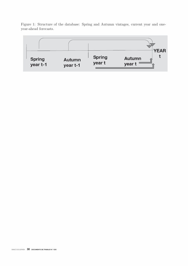
The vintage structure of the database is explained further in Figure 1. Following this
structure, we build up a database of forecasts for the government balance-to-GDP ratio
and real GDP growth, as published by the EC, the OECD and European governments in
real-time. In particular, EC projections have been taken from the different issues of the
publication European Economy (Supplement A, Economic Trends). For the OECD, the
source is the OECD Economic Outlook. Both the EC and the OECD publish projections
for Et[dt+1|St], Et[dt+1|At], Et+1[dt+1|St+1] and Et+1[dt+1|At+1]. As regards governments’
projections, the data have been compiled from two sources. On the one hand, data on
Et+1[dt+1|St+1] and Et+1[dt+1|At+1] have been taken from the EDP Notifications, submitted
twice a year (in Spring and Autumn) by European governments to the European Commission
in the framework of the so-called Excessive Deficit Procedure. On the other hand, data on
Et[dt+1|At] have been compiled from the Stability and Convergence Programmes submitted
by European governments to the European Commission.13 No figures are available for the
vintage Et[dt+1|St].
13EU countries send updated fiscal projections to the European Commission at least three time a year.Firstly, at the end of a given year (November/December) or the beginning of the next year (January)national fiscal authorities submit to the EC Stability and Convergence Programmes. These Programmesinclude multi-annual fiscal projections covering three to four years ahead. Secondly, national governmentssend to the EC in Spring of each year t the initial release of data for year t-1, and also take the opportunityto report updated projections for year t. Finally, the latter release of past data and estimates for the currentyear is updated in Autumn of each year.
14All over the study forecasts are lined up with the year in which the forecast was made, not the yearbeing forecast.
BANCO DE ESPAÑA 17 DOCUMENTO DE TRABAJO N.º 1233
The time period covered by our database is 1999-2007, and includes the 15 countries
members of the EU prior to the 2004 EU enlargement, namely Belgium, Germany, Greece,
Ireland, Spain, France, Italy, Luxembourg, Netherlands, Austria, Portugal, Finland, Den-
mark, Sweden, and the United Kingdom. All in all, taking into account certain missing
figures, the number of available observations for the four consecutive vintages [Et[dt+1|St],
Et[dt+1|At], Et+1[dt+1|St+1] and Et+1[dt+1|At+1]] is respectively [0,120,128,135] for govern-
ment’s projections, [120,120,135,135] for EC projections and [117,118,132,133] for OECD
projections.14
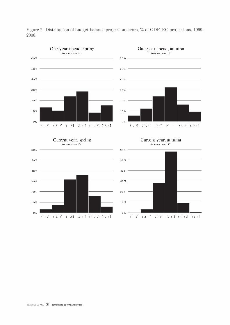
As an example of the reflection of the vintage structure in the data, Figure 2 shows the
distribution of government public deficit forecast errors computed from EC projections, for
the pool made of the 15 analyzed countries. It displays four projections for year t+1 public
balance, that differ in the selected forecast origin, the first one being the projection prepared
in spring of t for year t+1 (Et[dt+1|St]). The figure presents the statistical distribution of
projections errors and its evolution by vintage. The distribution of projection errors appears
to be slightly twisted to under-prediction of budget balances, which might be evidence for
the presence of bias in the pool. This seems to be particularly true for current year autumn
projections. In addition, there seems to be some evidence for increased accuracy across
consecutive vintages.
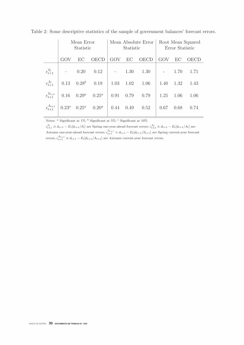
Table 2, in turn, shows some descriptive statistics of the real-time data set. Mean errors
over the whole sample were positive for GOV, EC and OECD projections, thus presenting a
small pessimistic positive bias (under-prediction of budget balances) over the years 1999 to
2007. Nevertheless, when accounting for variability, only the Autumn current year vintage
turned out to be statistically significant from zero in the case of the three institutions. The
optimistic bias was higher in size and statistically significant for the last three vintages in
the case of the EC and in the current-year vintages in the case of the OECD. Given that
the sample includes two upswing periods but only one downswing, this can be an indication
of a more prudent approach to government balance projections on the side of international
agencies. As regards the Mean Absolute Error and the RMSE statistics, also presented in
Table 2, two facts can be highlighted. First, accuracy improves with the information set, as
expected, given that both statistics get reduced as the information set gets closer to Autumn
BANCO DE ESPAÑA 18 DOCUMENTO DE TRABAJO N.º 1233
of the current year. Second, the size of forecast errors by the EC and OECD is commensurate
or lower than that of governments when looking at Autumn one-year-ahead forecasts and
Spring current-year ones; the estimates at the end of the current year (Autumn current-year
forecast), though, improve significantly in the case of GOV when compared with EC and
OECD estimates. This latter fact may reflect again the conservative bias on the side of
international agencies mentioned before, but also the existence of private information on the
side of GOV, most likely on current-year budgetary execution (and in particular as regards
expenditures).
3.2 Other variables
Along with the real-time database of government deficit forecasts, we also compile a parallel
real-time database of real GDP forecasts for the same organizations, taken from the same
publications in each case as with the budget balance projections. Errors committed when
forecasting macroeconomic variables are responsible for an important part of fiscal forecast
errors (see for example Leal et al., 2008) and thus it is natural to include GDP errors in the
analysis. For example, optimistic revenue forecasts tend to be associated to optimistic GDP
forecasts (Jonung and Larch, 2006).
As with political budget cycles – see for example Mink and de Haan (2005) – there
may be electoral, partisan or institutional forecast cycles. In the case of political forecast
cycles, policy makers deceive the public and the EC on their true budgetary position in
order to exploit the Phillips curve in the short-run. In an electoral forecast cycle, a given
election date determines government’s spending and taxation plans and the corresponding
information policy (see Alesina et al., 1998, and the references quoted therein). For example,
a government may increase spending prior to an election and hide the emerging budget
deficit, exploiting temporary information asymmetries. We aim at capturing these effects by
including country dummy variables that display a value of 1 in an election year and a zero
otherwise. We took the data from Armingeon et al. (2008) for the period 1999-2005, and
extended the variables by ourselves for 2006 and 2007.
The extant literature has shown that institutional variables are important determinants of
governments’ fiscal forecasting procedures and outcomes – see von Hagen (2010) or Beetsma
BANCO DE ESPAÑA 19 DOCUMENTO DE TRABAJO N.º 1233
et al. (2012) and the references quoted therein. Nevertheless, during the time period chosen
for our analysis (1999-2007) the fiscal framework was basically the same for all countries
included in the study, namely the SGP (and its reformed version in place since 2005). At
the same time, political institutions changed very little in the period 1999-2007 in the 15
EU countries considered. For these reasons the effect of fiscal rule indexes in extant studies
tend to be concealed by country fixed effects15. Given that the issue of fiscal institutions
is not core to our analysis and given also that country fixed effects are not rejected by our
empirical specifications, we decided to let the fixed effects of the models capture differences
in institutions across countries
4 Empirical strategy and results
4.1 Empirical strategy
Along the lines of the stylized equation discussed in (5), the baseline empirical equation we
estimate is as follows:
εht,i,j = δ0 + δ1 ELECt,i + δ2 εGDPt,i,j,h + δ3 DGOV
t,i,j,h +P∑
p=4
{δpDpt }+ ξt,i,j,h (7)
where εht,i,j is defined as in (6). {t, i, j, h} represent the four relevant sub-indexes: time,
country, institution and vintage of projection. i is the country index; j the institution index,
j = (GOV, EC, OECD); ELEC is a dummy for electoral periods, that is composed of
0’s (no election in year t in country i) and 1’s (every time year t is an election year in
country i); εGDP do refer to errors in forecasting real GDP of country i in year t incurred
by institution j at vintage h; DGOV is a dummy for government forecasts, that takes the
value of 1 if j = GOV ; h refers to the vintage of projections h = {St, At, St+1, At+1}. Dpt
represents additional dummy variables needed in the analysis, that will be detailed in due
time. Country-level fixed effects are also included in all regressions and control for differences
in budgetary procedures among countries, as discussed above.
15von Hagen (2010) analyzes the influence of fiscal institutions on budgetary deviations from governments’plans over the period 1999-2004 and decides to leave out country fixed-effects throughout his empirical study.The justification for this is that country fixed-effects would absorb, if introduced, the effect of institutionaldummies as institutions did not changed over the sample period.
BANCO DE ESPAÑA 20 DOCUMENTO DE TRABAJO N.º 1233
To correct for groupwise heteroskedasticity of error variances and cluster cross-correlation,
all regressions use estimators with cross-sectional, panel-corrected standard errors. Given
also that εGDP might likely be endogenous and thus correlated with the error term of the
regression, we decided to use a two-stages instrumental variable method (IV) henceforth.16
Given the characteristics of our dataset, controlling carefully for cross-correlation is crucial.
This is the case because in some regressions we include forecasts of different institutions for
the same country, and/or forecasts prepared by the same institution for different vintages.
Thus due account of clustering is implemented. As regards heteroskedasticity, some govern-
ments/international institutions may display more volatile deficit forecasts and more/less
accuracy.
4.2 Empirical results
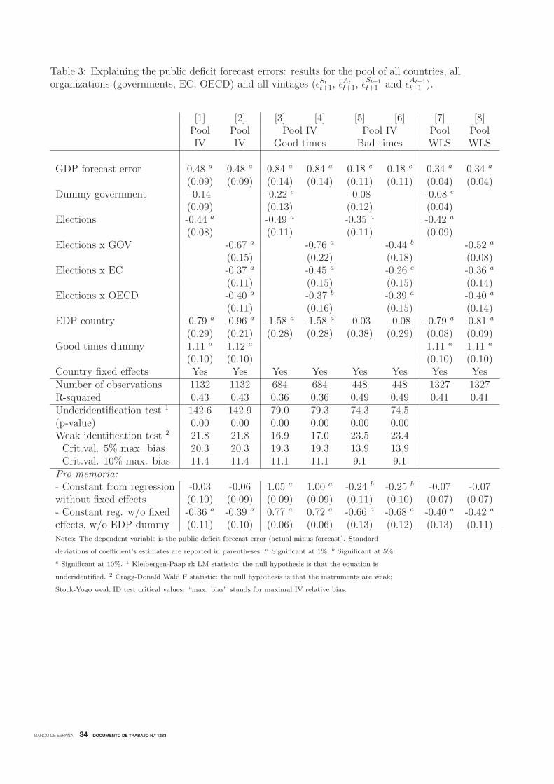
We show a first set of results for the pool of all countries, all institutions and all vintages.
These results are presented in Table 3 and constitute the most important set of results in
the paper. Column [1] of the table presents the results for the most comprehensive pool.
There, the dummy for government forecasts does not show up as statistically significant; this
means that, within the pool, the estimation method cannot distinguish forecast errors by
governments from those by the two international organizations in the sample. GDP errors
are significant and the average estimated point elasticity is 0.48, along the lines of related
studies; the positive sign says that a negative GDP growth shock produces ex-post opti-
mistic government revenue and budget balance forecasts. The dummy for elections years is
significantly different from zero and negative: it contributed to optimistic budget balance
forecasts. On average over all the dimensions considered, projections underestimated by 0.44
% of GDP actual government balances, i.e. public deficits turned out to be larger than fore-
seen. The regression also included two additional, control dummies. On the one hand, the
16Regressions are run using the ivreg2 command in STATA version 11. Using Weighted Least Squaresprovided similar results to those obtained by IV in some cases, and are thus presented in some tables forcomparability with related studies.
BANCO DE ESPAÑA 21 DOCUMENTO DE TRABAJO N.º 1233
dummy for governments of countries subject to an EDP procedure17 is negative and signifi-
cant, indicating that on average forecasts for EDP countries prepared more optimistic deficit
forecasts than non-EDP countries. On the other hand, a “good-times dummy” turned out
to be positive and significant, showing that forecasts tend to be on average more pessimistic
when the economic situation is buoyant than otherwise. Finally, it is worth mentioning
that if the estimation is conducted without fixed-effects and without the EDP dummy, a
significant and negative constant gets unveiled, a fact that makes explicit the presence of an
average optimistic bias in government balance projections.
As regards Column [2] of Table 3, it breaks down the impact of the election dummy by
institutions. Standard tests show that the coefficient of the interaction term “elections ×GOV” is significantly higher than the ones corresponding to the EC and the OECD. This can
be interpreted as a sign of more independent fiscal forecasts by international organizations.
Overall, WLS estimations shown in columns [7] and [8] display similar qualitative results to
those obtained by IV in columns [1] and [2].18
Still in Table 3, columns [3] to [6] present the same analysis as before but split into good
times and bad times. In bad times the peer and EU-wide institutional pressure might be
stronger and thus θ might be smaller than in good times, and also its variance σ2θ might be
smaller. On different grounds, in good times it might be easier for international organizations
to get governments to disclose their private information, so that ν should be smaller than
in bad times and thus international organizations might find it easier to differentiate their
forecasts from those of the governments. On the contrary, in bad times governments may
have more incentives to use it in a confidential way and thus EC and OECD projections
should be more difficult to be differentiated from those of the governments. In bad times,
thus, it should be more difficult to disentangle θ from ν, and then EC and OECD forecasts
17I.e. those countries within the sample that were subject to an Excessive Deficit Procedure, i.e. countriesthat exceeded the 3% of GDP public deficit dictated by EU fiscal rules at any time t within the sample 1999-2007. These countries are Germany, France, United Kingdom, Greece, Italy, Netherlands and Portugal.These countries might exhibit a differentiated behavior within the analyzed sample as they have been lessdisciplined while at the same time subject to peer pressure by the other EU countries and the EC.
18As regards all models estimated by IV, excluded instruments are lagged GDP errors and time dummies.It is worth noting that the underidentification tests show that all models are identified, i.e that the excludedinstruments are adequately correlated with the endogenous regressor. In addition, the weak instrumentstests show that the instruments are relevant.
BANCO DE ESPAÑA 22 DOCUMENTO DE TRABAJO N.º 1233
would tend to be closer to government’s ones. The most salient features of the empirical
estimations are, in this case, the following. First, fiscal forecasts turned out to be more
judgemental, i.e. less responsive to GDP errors, in bad times than in good times. This is
consistent with the usual approach to conduct discretionary policies more actively in times
of distress, typically by implementing expansionary measures at the beginning of a downturn
and implementing fiscal adjustment measures when public debt build-ups beyond certain,
sustainable limits. Second, governments display a distinct optimistic deficit bias in good
times (the “dummy government” is negative and significant), while in bad times they seem
to be more line with the other institutions. Third, bad times exert a kind of discipline
over EDP countries, as the relevant dummy is not significant in those periods. Fourth,
the negative influence of electoral cycles, even though being significant in both types of
periods, is more muted in bad times than in good times, and only in the latter periods are
international organizations clearly different from governments in this respect. Finally, with
all the caveats in interpretation, the constant term (when fixed-effects and EDP dummies
are excluded from the regressions) is negative in bad times (optimistic bias) and positive in
good times (conservative bias).
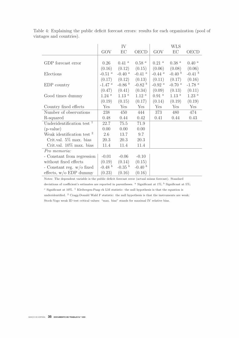
Table 4 shows results by organization (i.e. GOV, EC, and OECD). The most interesting
piece of additional evidence is related to the explanatory power of GDP forecast errors in
each case. Indeed, the coefficient associated to GOV is 0.26 (even though not significant at
the usual significance levels), below those estimated for the EC, 0.41, and OECD, 0.58. This
result indicates that, overall, governments’ fiscal balance projections are more judgemental
than those produced by international organizations, i.e. they tend to rely less on their
macroeconomic projections. Among the EC and the OECD, in the later case GDP forecast
errors account for a larger fraction of deficit forecast errors. In this table, though, one has to
consider that the weak instruments test shows evidence of weak identification in the case of
the GOV regression, and it is borderline in the case of OECD. WLS results, in turn, would
broadly confirm IV findings.
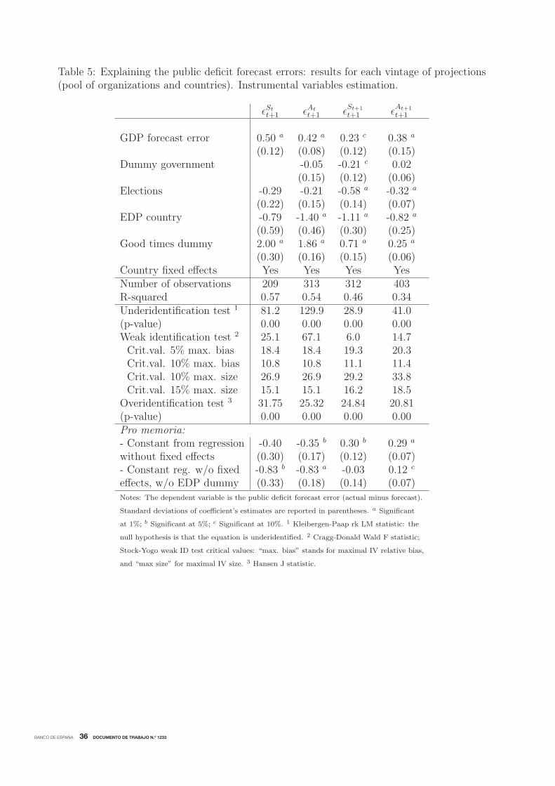
Finally, Table 5 disaggregate the information presented above by vintage of projections.
Some interesting insights can be highlighted: (i) the importance of errors in GDP as a ex-
planatory factor of public deficit errors decreases, in general, with the vintage, i.e. the closer
BANCO DE ESPAÑA 23 DOCUMENTO DE TRABAJO N.º 1233
the projection to the forecast year, revealing an increased GDP accuracy as the information
set gets increased, but also more weight on pure fiscal factors vs macro fundamentals in the
forecast process (like for example short-term data on budgetary execution); nevertheless,
the Spring current-year vintage is the one with the least weight on GDP errors, because it
benefits less from the first factor and at that point of the year still not enough from the
second; (ii) the dummy for electoral dates is negative for all vintages but it is only signif-
icant for the vintages with forecast origin within the year of the election; (iii) in the case
of the Spring current year vintage the dummy for government projections turns out to be
significant, showing an optimistic bias in Spring-current-year projections, that vanishes for
Autumn-current-year projections, the time of budget preparation; it is worth noticing that
it is in current year vintages in which the availability of private information is more rel-
evant, in particular as regards data on budgetary execution by sub-national governments;
(iv) the fixed effects country dummies (and the constant from the regression without fixed
effects) display a conservative bias for farther-from-the-forecast-origin vintages the forecast
year, with the size of the bias decreasing monotonically with the vintage. Overall, the Spring
current year vintage seems to be the one more judgemental and subject to political biases,
and this is precisely the vintage of projections published at the time of the year that is
most relevant from the point of view of implementing corrective fiscal measures in order to
guarantee that budgetary targets are met.
5 Conclusions
We provide empirical evidence on the existence of political economy determinants of inter-
national organizations’ (EC and OECD) fiscal forecasts for EU countries over the period
1999-2007. This evidence is based on a broad real-time database over a homogeneous time
period. We present evidence pointing to the fact that international agencies’ track record
of fiscal forecasts do present bias and correlation with electoral cycles in EU countries, even
though the latter is more mitigated than in the case of the governments, also in view of the
less judgemental projections of EC and OECD forecasts when compared with official ones.
More specifically, our main empirical results are as follows. First, we find that the influence
of electoral cycles on fiscal forecasts is significant in the case of governments (GOV), the
BANCO DE ESPAÑA 24 DOCUMENTO DE TRABAJO N.º 1233
European Commission (EC) and the OECD. Electoral cycles contribute to optimistic public
deficit forecasts. At the same time we find that the order of political independence is such
that: OECD and EC � GOV. Second, GDP errors influence significantly government deficit
errors, in such a way that a negative growth shock produces ex-post optimistic revenue and
deficit forecasts. GOV projections are found to be less reactive to the economic cycle (more
judgemental) than EC and OECD fiscal forecasts. Third, a dummy for government fiscal
projections in the pool of all datasets does not show up significantly different from zero,
but it does show up as significant and negative (i.e. consistent with a higher deficit bias) in
good times. Fourth, when the sample is spilt into good and bad times we find that elections
influence public deficit forecast errors more strongly in good than in bad times, and that
EC/OECD deficit projections become “more independent” in good times than in bad times.
We shed some light on the possible rationale of our empirical results by looking at a
simple, stylized model in which an independent agency tries to minimize the distance to
government’s forecast, given that that government’s information set includes private infor-
mation not available to the independent agency. When preparing their fiscal projections,
independent agency’s staff tries to grasp as much private information as possible from the
government, while at the same time have to disentangle ”political biases” from genuine ”pri-
vate information”. Thus, the presence of an inherited bias in international agencies’ fiscal
forecasts stems naturally in this set up.
The analysis and results of this paper do have important implications for the current
policy debate, specially in Europe. Institutional changes have to be implemented in the
procedures of elaboration of fiscal projections by international organizations if they are to
qualify as agencies in charge of the preparation of fiscal forecasts that could frame or tie
government’s fiscal forecasts, as international agencies’ fiscal forecasts have not been better
in the past than governmental ones. Possible institutional improvements include, on the one
hand, those aiming at improving transparency on fiscal data reporting (to minimize ex-ante
the ”private information bias” ν) and accountability (to minimize ex-ante the ”political bias”
θ) and, on the other hand, those increasing ex-ante pressure on misbehaving governments,
like the imposition of sanctions, given that a penalty on government’s fiscal forecast errors
may be helpful to minimize the ”private information” bias in government’s forecasts.
BANCO DE ESPAÑA 25 DOCUMENTO DE TRABAJO N.º 1233
References
Aldenhoff, F. O. (2007), “Are economic forecasts of the International Monetary Fund po-
litically biased? A public choice analysis”, Review of International Organizations, 2,
239-260.
Annett, A. (2006), “Enforcement and the Stability and Growth Pact: How Fiscal Policy
Did and Did Not Change Under Europe’s Fiscal Framework”, IMF Working Paper
2006/116.
Armingeon, K., Gerber, M., Leimgruber, P., Beyeler, M. and Menegale, S. (2008), “Code-
book: Comparative political data set I, 1960-2005”. Institute of Political Science,
University of Berne.
Artis, M. and Marcellino, M. (2001), “Fiscal forecasting: the track record of the IMF, the
OECD and the EC”, The Econometrics Journal, 4, S20-S36.
Artis, M. and Marcellino, M. (1998), “Fiscal solvency and fiscal forecasting in Europe”,
Centre for Economic Policy Research (CEPR), Discussion Paper no. 1836.
Auerbach, A.J. (1999), “On the Performance and Use of Government Revenue Forecasts”,
National Tax Journal, 52, 765-782.
Batchelor, R. (2001), “How useful are the forecasts of intergovernmental agencies? The
IMF and OECD versus the consensus”, Applied Economics, 33, 225-235.
Beetsma, R., B. Bluhm, M. Giuliodori and P. Wierts (2012), “From budgetary forecasts
to ex-post fiscal data: exploring the evolution of fiscal forecast errors in the EU”,
Contemporary Economic Policy, forthcoming.
Beetsma, R., M. Giuliodori and P. Wierts (2009), “Planning to Cheat: EU Fiscal Policy in
Real Time”, Economic Policy, 24, 753-804.
Blix, M., Wadefjord, J., Wienecke, U. and Adahl, M. (2001), “How good is the forecasting
performance of major institutions”, Economic Review No 3, Sveriges Risksbank.
BANCO DE ESPAÑA 26 DOCUMENTO DE TRABAJO N.º 1233
Boylan, R. T. (2008), “Political distortions in state forecasts”, Public Choice, 136, 41127.
Bretschneider, S.I., Gorr, W.L., Grizzle, G., and Klay, E. (1989), “Political and organiza-
tional influences on the accuracy of forecasting state government revenues”, Interna-
tional Journal of Forecasting, 5, 307-319.
Bruck, T., Stephan A. (2006), “Do Eurozone Countries Cheat with their Budget Deficit
Forecasts”, Kyklos, 59, 3-15.
Buti, M. and P. van den Noord (2004), “Fiscal policy in EMU: Rules, discretion and political
incentives”, European Economy - Economic Papers 206.
Christodoulakis, G. A. and E. C. Mamatzakis (2009), “Assessing the prudence of economic
forecasts in the EU”, Journal of Applied Econometrics, 24, 583-606.
Debrun, X., Hauner, D. and Kumar, M. S. (2009), “Independent fiscal agencies”, Journal
of Economic Surveys, 23, 44-81.
Dreher, A., Marchesi, S., Vreeland, J. R. (2008), “The political economy of IMF forecasts”,
Public Choice, 137, 145-171.
European Commission (2006), “Part III: National numerical fiscal rules and institutions for
sound public finances”, pp. 135-195 in ”Public finances in EMU”, European Economy,
No 3.
Frankel, J. A. (2011), “Over-optimism in forecasts by official budget agencies and its im-
plications”, NBER Working Papers 17239, July.
Grizzle, G. A. and W. E. Klay (1994), “Forecasting State Sales Tax revenues: comparing
the accuracy of different methods”, State and Local Government Review, 26, 142-152.
Hallerberg, M., Strauch, R. and von Hagen, J. (2007), “The design of fiscal rules and forms
of governance in European Union countries”, European Journal of Political Economy,
23, 338-359.
Jonung, L., and Larch, M. (2006), “Fiscal policy in the EU: are official output forecasts
biased?”, Economic Policy, July, 491-534.
BANCO DE ESPAÑA 27 DOCUMENTO DE TRABAJO N.º 1233
Keereman, F. (1999), “The track record of Commission Forecasts”, European Commission
Economic Papers, n. 137.
Larch, M., P. Van den Noord, and L. Jonung (2010), “The stability and growth pact: lessons
from the great recession”, MPRA Paper No. 27900.
Leal, T., Perez, J. J., Tujula, M. and Vidal, J.-P. (2008) “Fiscal forecasting: lessons from
the literature and challenges”, Fiscal Studies, 29, 347-386.
Leeper, E. M. (2009), “Anchoring Fiscal Expectations”, NBER Working Papers 15269.
Marinheiro, C. F. (2010), “Fiscal sustainability and the accuracy of macroeconomic fore-
casts: do supranational forecasts rather than government forecasts make a difference?”,
GEMF Working Papers 2010, 7, Faculty of Economics, University of Coimbra.
Melander, A., Sismanidis, G. and Grenouilleau, D. (2007), “The track record of the Commis-
sion’s forecasts - an update”, European Economy Economic Papers, No 291, October.
Mink, M., and J. de Haan (2005), “Has the Stability and Growth Pact Impeded Political
Budget Cycles in the European Union?”, CESifo Working Paper Series, 1532.
Moulin, L., and Wierts, P. (2006), “How Credible are Multiannual Budgetary Plans in the
EU?”, in Fiscal Indicators, pp. 983-1005, Banca d’Italia.
Pina, A. and N. Venes (2011), “The political economy of EDP fiscal forecasts: an empirical
assessment”, European Journal of Political Economy, 27, 534-546.
Pons, J. (2000), “The accuracy of IMF and OECD forecasts for G-7 countries”, Journal of
Forecasting, 19, 53-63.
Poplawski-Ribeiro, M. and Rulke, J.-C. (2010), “Fiscal expectations and the Stability and
Growth Pact: evidence from survey data”, CEPII Working Paper No 2010-05, March.
Strauch, R., Hallerberg, M., von Hagen, J. (2004), “Budgetary Forecasts in Europe - The
Track Record of Stability and Covergence Programmes”, European Central Bank WP
307.
BANCO DE ESPAÑA 28 DOCUMENTO DE TRABAJO N.º 1233
Timmermann, A. (2007), “An evaluation of the World Economic Outlook forecasts”, IMF
Staff Papers, 54, 1-33.
von Hagen, J. (2010), “Sticking to fiscal plans: the role of institutions”, Public Choice, 144,
487-503.
Wyplosz, C. (2008), “Fiscal policy councils: Unlovable or just unloved”, Swedish Economic
Policy Review, 15, 173-192.
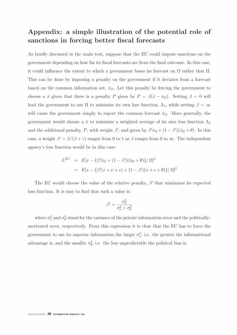
BANCO DE ESPAÑA 29 DOCUMENTO DE TRABAJO N.º 1233
Appendix: a simple illustration of the potential role of
sanctions in forcing better fiscal forecasts
As briefly discussed in the main text, suppose that the EC could impose sanctions on the
government depending on how far its fiscal forecasts are from the final outcome. In this case,
it could influence the extent to which a government bases its forecast on Ω rather that Π.
This can be done by imposing a penalty on the government if it deviates from a forecast
based on the common information set, xΩ. Let this penalty be forcing the government to
choose a x given that there is a penalty P given by P = β(x − xΩ). Setting β = 0 will
lead the government to use Π to minimize its own loss function, Λ1, while setting β = ∞will cause the government simply to report the common forecast xΩ. More generally, the
government would choose a x to minimize a weighted average of its own loss function Λ2
and the additional penalty, P , with weight β′, and given by β′xΩ + (1− β′)(xΠ + θ). In this
case, a weight β′ = β/(β + γ) ranges from 0 to 1 as β ranges from 0 to ∞. The independent
agency’s loss function would be in this case:
LEC = E[x− {β′xΩ + (1− β′)(xΠ + θ)}| Ω]2
= E[x− {β′(x+ ν + ε) + (1− β′)(x+ ε+ θ)}| Ω]2
The EC would choose the value of the relative penalty, β′ that minimizes its expected
loss function. It is easy to find that such a value is:
β′ =σ2θ
σ2ν + σ2
θ
where σ2ν and σ2
θ stand for the variance of the private information error and the politically-
motivated error, respectively. From this expression it is clear that the EC has to force the
government to use its superior information the larger σ2ν , i.e. the greater the informational
advantage is, and the smaller σ2θ , i.e. the less unpredictable the political bias is.
BANCO DE ESPAÑA 30 DOCUMENTO DE TRABAJO N.º 1233
Figure 1: Structure of the database: Spring and Autumn vintages, current year and one-year-ahead forecasts.
BANCO DE ESPAÑA 31 DOCUMENTO DE TRABAJO N.º 1233
Figure 2: Distribution of budget balance projection errors, % of GDP. EC projections, 1999-2006.
BANCO DE ESPAÑA 32 DOCUMENTO DE TRABAJO N.º 1233
Table 1: Some related literature analyzing public deficit forecast errors in EU countries.
Main papers and Information Type of Forecasts of organization:time periods covered source analysis f EC OECD Governments
Strauch et al. (2004) National a Econometric – – Autumn j-period-ahead
1991-2002 forecasts, j = 0, 1, 2
Bruck & Stephan (2006) EC b Econometric – – Autumn j-period-ahead
1995-2003 forecasts, j = 1
von Hagen (2010) Nationala Econometric – – Autumn j-period-ahead
1999-2004 forecasts, j = 0, 1, 2
Pina & Venes (2011) National Econometric – – Spring and Autumn
1994-2006 EDP ccurrent year forecasts
Annet (2006) National a Econometric – – Autumn j-period-ahead
1980-2004 forecasts, j = 1
Moulin & Wierts (2006) National a Econometric – – Autumn j-period-ahead
1998-2005 forecasts, j = 1
Beetsma et al. (2012) National a Econometric – – Autumn j-period-ahead
1998-2008 forecasts, j = 0, 1, 2
Artis & Marcellino (2001) EC b, Descriptive All All –1975-1995 e OECD d vintages vintages
Keereman (1999) EC b Descriptive All – –1970-1997 vintages
Melander et al. (2007) EC b Descriptive All – –1970-2005 vintages
Marinheiro (2010) EC b Descriptive All – –1999-2007 vintages
Notes: a National sources: Stability and Convergence Programmes by EU Member States.
b European Commission, several vintages of the publication ”European Economy- Economic Forecasts”.
c EDP reports: Excessive Deficit Procedure reports.
d OECD Economic Outlook.
e Their analysis also covers IMF projections (World Economic Outlook).
f “Descriptive” refers to the implementation of standard measures of forecast accuracy, including directional accuracy, plus
traditional bias and efficiency tests. ”Econometric” refers to the inclusion of economic, political and/or institutional variables
as explanatory variables. “All vintages” refers to Spring and Autumn current year and year-ahead forecasts.
BANCO DE ESPAÑA 33 DOCUMENTO DE TRABAJO N.º 1233
Table 2: Some descriptive statistics of the sample of government balances’ forecast errors.
Mean Error Mean Absolute Error Root Mean SquaredStatistic Statistic Error Statistic
GOV EC OECD GOV EC OECD GOV EC OECD
εStt+1 – 0.20 0.12 – 1.30 1.30 - 1.70 1.71
εAtt+1 0.13 0.28b 0.19 1.03 1.02 1.06 1.40 1.32 1.43
εSt+1
t+1 0.16 0.29a 0.25a 0.91 0.79 0.79 1.25 1.06 1.06
εAt+1
t+1 0.23a 0.25a 0.20a 0.44 0.49 0.52 0.67 0.68 0.74
Notes: a Significant at 1%; b Significant at 5%; c Significant at 10%.
εStt+1 ≡ dt+1 − Et[dt+1/St] are Spring one-year-ahead forecast errors; εAt
t+1 ≡ dt+1 − Et[dt+1/At] are
Autumn one-year-ahead forecast errors; εSt+1t+1 ≡ dt+1 − Et[dt+1/St+1] are Spring current-year forecast
errors; εAt+1t+1 ≡ dt+1 − Et[dt+1/At+1] are Autumn current-year forecast errors.
BANCO DE ESPAÑA 34 DOCUMENTO DE TRABAJO N.º 1233
Table 3: Explaining the public deficit forecast errors: results for the pool of all countries, allorganizations (governments, EC, OECD) and all vintages (εSt
t+1, εAtt+1, ε
St+1
t+1 and εAt+1
t+1 ).
[1] [2] [3] [4] [5] [6] [7] [8]Pool Pool Pool IV Pool IV Pool PoolIV IV Good times Bad times WLS WLS
GDP forecast error 0.48 a 0.48 a 0.84 a 0.84 a 0.18 c 0.18 c 0.34 a 0.34 a
(0.09) (0.09) (0.14) (0.14) (0.11) (0.11) (0.04) (0.04)Dummy government -0.14 -0.22 c -0.08 -0.08 c
(0.09) (0.13) (0.12) (0.04)Elections -0.44 a -0.49 a -0.35 a -0.42 a
(0.08) (0.11) (0.11) (0.09)Elections x GOV -0.67 a -0.76 a -0.44 b -0.52 a
(0.15) (0.22) (0.18) (0.08)Elections x EC -0.37 a -0.45 a -0.26 c -0.36 a
(0.11) (0.15) (0.15) (0.14)Elections x OECD -0.40 a -0.37 b -0.39 a -0.40 a
(0.11) (0.16) (0.15) (0.14)EDP country -0.79 a -0.96 a -1.58 a -1.58 a -0.03 -0.08 -0.79 a -0.81 a
(0.29) (0.21) (0.28) (0.28) (0.38) (0.29) (0.08) (0.09)Good times dummy 1.11 a 1.12 a 1.11 a 1.11 a
(0.10) (0.10) (0.10) (0.10)Country fixed effects Yes Yes Yes Yes Yes Yes Yes YesNumber of observations 1132 1132 684 684 448 448 1327 1327R-squared 0.43 0.43 0.36 0.36 0.49 0.49 0.41 0.41Underidentification test 1 142.6 142.9 79.0 79.3 74.3 74.5(p-value) 0.00 0.00 0.00 0.00 0.00 0.00Weak identification test 2 21.8 21.8 16.9 17.0 23.5 23.4Crit.val. 5% max. bias 20.3 20.3 19.3 19.3 13.9 13.9Crit.val. 10% max. bias 11.4 11.4 11.1 11.1 9.1 9.1
Pro memoria:- Constant from regression -0.03 -0.06 1.05 a 1.00 a -0.24 b -0.25 b -0.07 -0.07without fixed effects (0.10) (0.09) (0.09) (0.09) (0.11) (0.10) (0.07) (0.07)- Constant reg. w/o fixed -0.36 a -0.39 a 0.77 a 0.72 a -0.66 a -0.68 a -0.40 a -0.42 a
effects, w/o EDP dummy (0.11) (0.10) (0.06) (0.06) (0.13) (0.12) (0.13) (0.11)Notes: The dependent variable is the public deficit forecast error (actual minus forecast). Standard
deviations of coefficient’s estimates are reported in parentheses. a Significant at 1%; b Significant at 5%;
c Significant at 10%. 1 Kleibergen-Paap rk LM statistic: the null hypothesis is that the equation is
underidentified. 2 Cragg-Donald Wald F statistic: the null hypothesis is that the instruments are weak;
Stock-Yogo weak ID test critical values: “max. bias” stands for maximal IV relative bias.
BANCO DE ESPAÑA 35 DOCUMENTO DE TRABAJO N.º 1233
Table 4: Explaining the public deficit forecast errors: results for each organization (pool ofvintages and countries).
IV WLSGOV EC OECD GOV EC OECD
GDP forecast error 0.26 0.41 a 0.58 a 0.21 a 0.38 a 0.40 a
(0.16) (0.12) (0.15) (0.06) (0.08) (0.06)Elections -0.51 a -0.40 a -0.41 a -0.44 a -0.40 b -0.41 b
(0.17) (0.12) (0.13) (0.11) (0.17) (0.16)EDP country -1.47 a -0.86 b -0.82 b -0.92 a -0.70 a -1.78 a
(0.47) (0.41) (0.34) (0.09) (0.13) (0.11)Good times dummy 1.24 a 1.13 a 1.12 a 0.91 a 1.13 a 1.23 a
(0.19) (0.15) (0.17) (0.14) (0.19) (0.19)Country fixed effects Yes Yes Yes Yes Yes YesNumber of observations 238 450 444 373 480 474R-squared 0.48 0.44 0.42 0.41 0.44 0.43Underidentification test 1 22.7 75.5 71.9(p-value) 0.00 0.00 0.00Weak identification test 2 2.6 13.7 9.7Crit.val. 5% max. bias 20.3 20.3 20.3Crit.val. 10% max. bias 11.4 11.4 11.4
Pro memoria:- Constant from regression -0.01 -0.06 -0.10without fixed effects (0.19) (0.14) (0.15)- Constant reg. w/o fixed -0.48 b -0.35 b -0.40 b
effects, w/o EDP dummy (0.23) (0.16) (0.16)Notes: The dependent variable is the public deficit forecast error (actual minus forecast). Standard
deviations of coefficient’s estimates are reported in parentheses. a Significant at 1%; b Significant at 5%;
c Significant at 10%. 1 Kleibergen-Paap rk LM statistic: the null hypothesis is that the equation is
underidentified. 2 Cragg-Donald Wald F statistic: the null hypothesis is that the instruments are weak;
Stock-Yogo weak ID test critical values: “max. bias” stands for maximal IV relative bias.
BANCO DE ESPAÑA 36 DOCUMENTO DE TRABAJO N.º 1233
Table 5: Explaining the public deficit forecast errors: results for each vintage of projections(pool of organizations and countries). Instrumental variables estimation.
εStt+1 εAt
t+1 εSt+1
t+1 εAt+1
t+1
GDP forecast error 0.50 a 0.42 a 0.23 c 0.38 a
(0.12) (0.08) (0.12) (0.15)Dummy government -0.05 -0.21 c 0.02
(0.15) (0.12) (0.06)Elections -0.29 -0.21 -0.58 a -0.32 a
(0.22) (0.15) (0.14) (0.07)EDP country -0.79 -1.40 a -1.11 a -0.82 a
(0.59) (0.46) (0.30) (0.25)Good times dummy 2.00 a 1.86 a 0.71 a 0.25 a
(0.30) (0.16) (0.15) (0.06)Country fixed effects Yes Yes Yes YesNumber of observations 209 313 312 403R-squared 0.57 0.54 0.46 0.34Underidentification test 1 81.2 129.9 28.9 41.0(p-value) 0.00 0.00 0.00 0.00Weak identification test 2 25.1 67.1 6.0 14.7Crit.val. 5% max. bias 18.4 18.4 19.3 20.3Crit.val. 10% max. bias 10.8 10.8 11.1 11.4Crit.val. 10% max. size 26.9 26.9 29.2 33.8Crit.val. 15% max. size 15.1 15.1 16.2 18.5
Overidentification test 3 31.75 25.32 24.84 20.81(p-value) 0.00 0.00 0.00 0.00Pro memoria:- Constant from regression -0.40 -0.35 b 0.30 b 0.29 a
without fixed effects (0.30) (0.17) (0.12) (0.07)- Constant reg. w/o fixed -0.83 b -0.83 a -0.03 0.12 c
effects, w/o EDP dummy (0.33) (0.18) (0.14) (0.07)Notes: The dependent variable is the public deficit forecast error (actual minus forecast).
Standard deviations of coefficient’s estimates are reported in parentheses. a Significant
at 1%; b Significant at 5%; c Significant at 10%. 1 Kleibergen-Paap rk LM statistic: the
null hypothesis is that the equation is underidentified. 2 Cragg-Donald Wald F statistic;
Stock-Yogo weak ID test critical values: “max. bias” stands for maximal IV relative bias,
and “max size” for maximal IV size. 3 Hansen J statistic.
BANCO DE ESPAÑA PUBLICATIONS
WORKING PAPERS
1101 GIACOMO MASIER and ERNESTO VILLANUEVA: Consumption and initial mortgage conditions: evidence from survey
data.
1102 PABLO HERNÁNDEZ DE COS and ENRIQUE MORAL-BENITO: Endogenous fi scal consolidations
1103 CÉSAR CALDERÓN, ENRIQUE MORAL-BENITO and LUIS SERVÉN: Is infrastructure capital productive? A dynamic
heterogeneous approach.
1104 MICHAEL DANQUAH, ENRIQUE MORAL-BENITO and BAZOUMANA OUATTARA: TFP growth and its determinants:
nonparametrics and model averaging.
1105 JUAN CARLOS BERGANZA and CARMEN BROTO: Flexible infl ation targets, forex interventions and exchange rate
volatility in emerging countries.
1106 FRANCISCO DE CASTRO, JAVIER J. PÉREZ and MARTA RODRÍGUEZ VIVES: Fiscal data revisions in Europe.
1107 ANGEL GAVILÁN, PABLO HERNÁNDEZ DE COS, JUAN F. JIMENO and JUAN A. ROJAS: Fiscal policy, structural
reforms and external imbalances: a quantitative evaluation for Spain.
1108 EVA ORTEGA, MARGARITA RUBIO and CARLOS THOMAS: House purchase versus rental in Spain.
1109 ENRIQUE MORAL-BENITO: Dynamic panels with predetermined regressors: likelihood-based estimation and Bayesian
averaging with an application to cross-country growth.
1110 NIKOLAI STÄHLER and CARLOS THOMAS: FiMod – a DSGE model for fi scal policy simulations.
1111 ÁLVARO CARTEA and JOSÉ PENALVA: Where is the value in high frequency trading?
1112 FILIPA SÁ and FRANCESCA VIANI: Shifts in portfolio preferences of international investors: an application to sovereign
wealth funds.
1113 REBECA ANGUREN MARTÍN: Credit cycles: Evidence based on a non-linear model for developed countries.
1114 LAURA HOSPIDO: Estimating non-linear models with multiple fi xed effects: A computational note.
1115 ENRIQUE MORAL-BENITO and CRISTIAN BARTOLUCCI: Income and democracy: Revisiting the evidence.
1116 AGUSTÍN MARAVALL HERRERO and DOMINGO PÉREZ CAÑETE: Applying and interpreting model-based seasonal
adjustment. The euro-area industrial production series.
1117 JULIO CÁCERES-DELPIANO: Is there a cost associated with an increase in family size beyond child investment?
Evidence from developing countries.
1118 DANIEL PÉREZ, VICENTE SALAS-FUMÁS and JESÚS SAURINA: Do dynamic provisions reduce income smoothing
using loan loss provisions?
1119 GALO NUÑO, PEDRO TEDDE and ALESSIO MORO: Money dynamics with multiple banks of issue: evidence from
Spain 1856-1874.
1120 RAQUEL CARRASCO, JUAN F. JIMENO and A. CAROLINA ORTEGA: Accounting for changes in the Spanish wage
distribution: the role of employment composition effects.
1121 FRANCISCO DE CASTRO and LAURA FERNÁNDEZ-CABALLERO: The effects of fi scal shocks on the exchange rate in
Spain.
1122 JAMES COSTAIN and ANTON NAKOV: Precautionary price stickiness.
1123 ENRIQUE MORAL-BENITO: Model averaging in economics.
1124 GABRIEL JIMÉNEZ, ATIF MIAN, JOSÉ-LUIS PEYDRÓ AND JESÚS SAURINA: Local versus aggregate lending
channels: the effects of securitization on corporate credit supply.
1125 ANTON NAKOV and GALO NUÑO: A general equilibrium model of the oil market.
1126 DANIEL C. HARDY and MARÍA J. NIETO: Cross-border coordination of prudential supervision and deposit guarantees.
1127 LAURA FERNÁNDEZ-CABALLERO, DIEGO J. PEDREGAL and JAVIER J. PÉREZ: Monitoring sub-central government
spending in Spain.
1128 CARLOS PÉREZ MONTES: Optimal capital structure and regulatory control.
1129 JAVIER ANDRÉS, JOSÉ E. BOSCÁ and JAVIER FERRI: Household debt and labour market fl uctuations.
1130 ANTON NAKOV and CARLOS THOMAS: Optimal monetary policy with state-dependent pricing.
1131 JUAN F. JIMENO and CARLOS THOMAS: Collective bargaining, fi rm heterogeneity and unemployment.
1132 ANTON NAKOV and GALO NUÑO: Learning from experience in the stock market.
1133 ALESSIO MORO and GALO NUÑO: Does TFP drive housing prices? A growth accounting exercise for four countries.
1201 CARLOS PÉREZ MONTES: Regulatory bias in the price structure of local telephone services.
1202 MAXIMO CAMACHO, GABRIEL PEREZ-QUIROS and PILAR PONCELA: Extracting non-linear signals from several
economic indicators.
1203 MARCOS DAL BIANCO, MAXIMO CAMACHO and GABRIEL PEREZ-QUIROS: Short-run forecasting of the euro-dollar
exchange rate with economic fundamentals.
1204 ROCIO ALVAREZ, MAXIMO CAMACHO and GABRIEL PEREZ-QUIROS: Finite sample performance of small versus
large scale dynamic factor models.
1205 MAXIMO CAMACHO, GABRIEL PEREZ-QUIROS and PILAR PONCELA: Markov-switching dynamic factor models in
real time.
1206 IGNACIO HERNANDO and ERNESTO VILLANUEVA: The recent slowdown of bank lending in Spain: are supply-side
factors relevant?
1207 JAMES COSTAIN and BEATRIZ DE BLAS: Smoothing shocks and balancing budgets in a currency union.
1208 AITOR LACUESTA, SERGIO PUENTE and ERNESTO VILLANUEVA: The schooling response to a sustained Increase in
low-skill wages: evidence from Spain 1989-2009.
1209 GABOR PULA and DANIEL SANTABÁRBARA: Is China climbing up the quality ladder?
1210 ROBERTO BLANCO and RICARDO GIMENO: Determinants of default ratios in the segment of loans to households in
Spain.
1211 ENRIQUE ALBEROLA, AITOR ERCE and JOSÉ MARÍA SERENA: International reserves and gross capital fl ows.
Dynamics during fi nancial stress.
1212 GIANCARLO CORSETTI, LUCA DEDOLA and FRANCESCA VIANI: The international risk-sharing puzzle is at business-
cycle and lower frequency.
1213 FRANCISCO ALVAREZ-CUADRADO, JOSE MARIA CASADO, JOSE MARIA LABEAGA and DHANOOS
SUTTHIPHISAL: Envy and habits: panel data estimates of interdependent preferences.
1214 JOSE MARIA CASADO: Consumption partial insurance of Spanish households.
1215 J. ANDRÉS, J. E. BOSCÁ and J. FERRI: Household leverage and fi scal multipliers.
1216 JAMES COSTAIN and BEATRIZ DE BLAS: The role of fi scal delegation in a monetary union: a survey of the political
economy issues.
1217 ARTURO MACÍAS and MARIANO MATILLA-GARCÍA: Net energy analysis in a Ramsey-Hotelling growth model.
1218 ALFREDO MARTÍN-OLIVER, SONIA RUANO and VICENTE SALAS-FUMÁS: Effects of equity capital on the interest rate
and the demand for credit. Empirical evidence from Spanish banks.
1219 PALOMA LÓPEZ-GARCÍA, JOSÉ MANUEL MONTERO and ENRIQUE MORAL-BENITO: Business cycles and
investment in intangibles: evidence from Spanish fi rms.
1220 ENRIQUE ALBEROLA, LUIS MOLINA andPEDRO DEL RÍO: Boom-bust cycles, imbalances and discipline in Europe.
1221 CARLOS GONZÁLEZ-AGUADO and ENRIQUE MORAL-BENITO: Determinants of corporate default: a BMA approach.
1222 GALO NUÑO and CARLOS THOMAS: Bank leverage cycles.
1223 YUNUS AKSOY and HENRIQUE S. BASSO: Liquidity, term spreads and monetary policy.
1224 FRANCISCO DE CASTRO and DANIEL GARROTE: The effects of fi scal shocks on the exchange rate in the EMU and
differences with the US.
1225 STÉPHANE BONHOMME and LAURA HOSPIDO: The cycle of earnings inequality: evidence from Spanish social
security data.
1226 CARMEN BROTO: The effectiveness of forex interventions in four Latin American countries.
1227 LORENZO RICCI and DAVID VEREDAS: TailCoR.
1228 YVES DOMINICY, SIEGFRIED HÖRMANN, HIROAKI OGATA and DAVID VEREDAS: Marginal quantiles for stationary
processes.
1229 MATTEO BARIGOZZI, ROXANA HALBLEIB and DAVID VEREDAS: Which model to match?
1230 MATTEO LUCIANI and DAVID VEREDAS: A model for vast panels of volatilities.
1231 AITOR ERCE: Does the IMF’s offi cial support affect sovereign bond maturities?
1232 JAVIER MENCÍA and ENRIQUE SENTANA: Valuation of VIX derivatives.
1233 ROSSANA MEROLA and JAVIER J. PÉREZ: Fiscal forecast errors: governments vs independent agencies?
Unidad de Servicios AuxiliaresAlcalá, 48 - 28014 Madrid
Telephone +34 91 338 6360 E-mail: [email protected]
www.bde.es


![[ENTER] - Sacramento Area Council of Governments](https://img.pdfslide.net/doc/110x75/6332bd753108fad7760ec187/enter-sacramento-area-council-of-governments.jpg)


