Embed Size (px)
Citation preview
Fitness Landscapes and Evolvability
Tom Smith [email protected] for Computational Neuroscience and Robotics, School of Biological Sciences,University of Sussex, Brighton, UK
Phil Husbands [email protected] for Computational Neuroscience and Robotics, School of Cognitive andComputing Sciences, University of Sussex, Brighton, UK
Paul Layzell paul [email protected] Laboratories, Bristol, UK
Michael O’Shea [email protected] for Computational Neuroscience and Robotics, School of Biological Sciences,University of Sussex, Brighton, UK
AbstractIn this paper, we develop techniques based on evolvability statistics of the fitness land-scape surrounding sampled solutions. Averaging the measures over a sample of equalfitness solutions allows us to build up fitness evolvability portraits of the fitness land-scape, which we show can be used to compare both the ruggedness and neutrality in aset of tunably rugged and tunably neutral landscapes. We further show that the tech-niques can be used with solution samples collected through both random samplingof the landscapes and online sampling during optimization. Finally, we apply thetechniques to two real evolutionary electronics search spaces and highlight differencesbetween the two search spaces, comparing with the time taken to find good solutionsthrough search.
KeywordsEvolvability, fitness landscape, search space, neutral evolution, NK system, evolution-ary electronics.
1 Introduction
In this paper, we develop novel techniques based on local characteristics of the fitnesslandscape surrounding a solution. Averaging over a sample of equal fitness solutionsallows us to build up fitness evolvability portraits of the fitness landscape, which we showcan be used to compare both the ruggedness and neutrality in a set of tunably ruggedand tunably neutral landscapes.
A feature of most fitness landscape descriptions is that a single global metric, e.g.,correlation lengths, is used to describe the entire fitness landscape. The techniquespresented in this paper develop a set of continuous metrics that vary with solutionfitness. This approach allows fitness landscape features to be investigated at differentfitness levels, leading to a fuller description of the space.
Many problems to which stochastic search techniques such as evolutionary com-putation are typically applied, present such highly skewed distributions of solution fit-nesses that random sampling (even when some imposed distribution is applied to the
c©2002 by the Massachusetts Institute of Technology Evolutionary Computation 10(1): 1-34
T. Smith et al.
sample) is unlikely to represent fitnesses above a given level, even when such fitnessesare easily found through direct search optimization. In such spaces, we must developdescriptions that work with samples collected using online sampling techniques (in theremainder of the paper, we will use the term online sample to refer to samples collectedduring some search process, as opposed to samples collected through random sam-pling). We show that the fitness evolvability portraits presented work with samplesof solutions collected both through random sampling techniques and through onlinesampling of the best solution so far found during simple hill-climbing optimization.
Finally, we investigate the application of the fitness evolvability portraits to a realevolutionary electronics problem, namely optimization of digital inverter circuits. Weshow that the portraits can be used to compare two different solution mappings, high-lighting differences between the two search spaces and comparing the time taken tofind good solutions through search.
The paper proceeds as follows: Section 2 outlines the concepts of fitness landscapesand neutrality and describes the relationship between problem difficulty and fitnesslandscape structure. Section 3 introduces the notion of solution evolvability as definedby local characteristics of the fitness landscape surrounding the solution and derivesand applies the fitness evolvability portraits used in the remainder of the paper. Sec-tion 4 describes the tunably rugged and tunably neutral terraced NK landscapes usedas test problems in this work. Sections 5 and 6 use the portraits derived in Section 3to describe the test landscapes and show that they can be used to compare the rugged-ness and neutrality in the tunably rugged and tunably neutral landscapes. Section 7investigates the case where the fitness evolvability portraits are derived from solutionsamples collected during simple hill-climbing, showing that the portraits are robustto such online sampling. Finally, two real evolutionary electronics search spaces areinvestigated in Section 8, and the paper closes with discussion.
2 Fitness Landscapes and Neutrality
This section introduces two of the main concepts used in the paper. The fitness landscape(Section 2.1), first introduced by Wright (1932), describes the search space as a multidi-mensional landscape defined by the genotype-to-fitness mapping through which evo-lution moves. The classical idea of searching this landscape for good genotypes focuseson the difficulty of climbing up to the globally optimal fitness solution and avoidinglocally optimal solutions. Here we argue that in difficult search problems, much ofthe time may be spent in nonadaptive neutral evolution (Section 2.2). Thus techniquesaimed at describing the space in some way, must take account of the neutrality in thespace. Section 2.3 describes how the difficulty of finding good solutions is determinedby the structure of the fitness landscape, and Section 2.4 outlines different methods forsampling the fitness landscape structure.
2.1 Fitness Landscapes
Wright (1932) introduced the fitness landscape as a nonmathematical aid to visualizethe action during evolution of selection and variation (in this paper, we will use theterm evolution to refer to both natural biological evolution and the artificial evolutionclass of stochastic search processes that operate through some form of “generate-and-test” algorithm, e.g., genetic algorithms (Holland, 1992), genetic programming (Koza,1992), evolutionary strategies (Rechenberg, 1973), and evolutionary programming (Fo-gel et al., 1966)). The description views the space in which evolution takes place as alandscape, with one dimension per genotype locus and an extra dimension, or height,
2 Evolutionary Computation Volume 10, Number 1
Fitness Landscapes and Evolvability
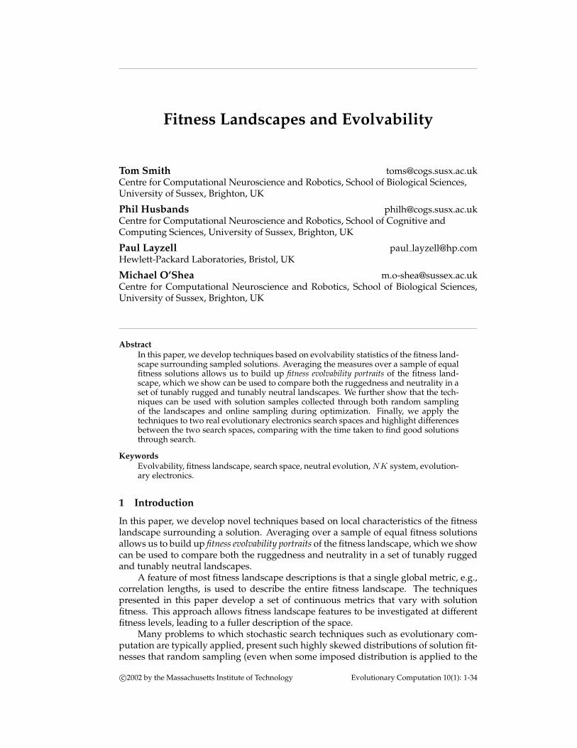
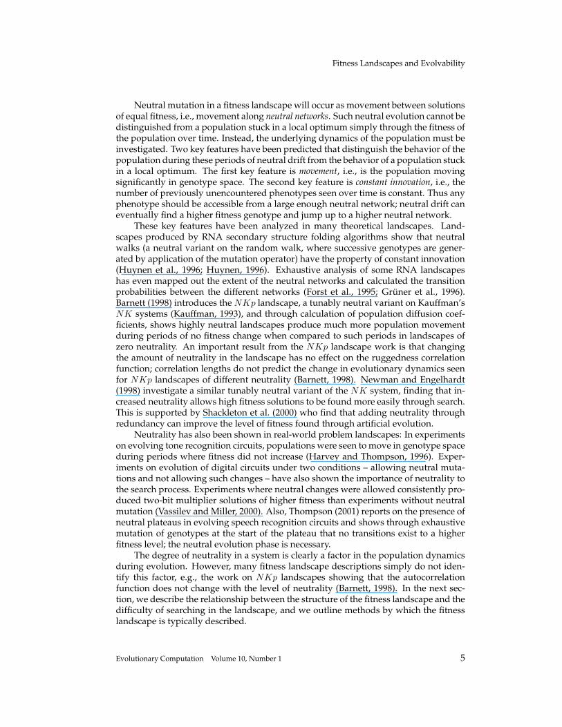
Figure 1: A two-dimensional model fitness landscape with one globally-optimal andone locally-optimal peak. From a starting point chosen at random, the search processtries to find good solutions. The process creates a new set of solutions through theapplication of genetic operators to the current solution(s), evaluating whether the newset is better than the current solutions. Evolving populations will tend to get stuck atthe locally-optimal peak due to its large basin of attraction, and from there will onlyfind the global optimum with difficulty.
representing the phenotype, or fitness, of that particular genotype.1 The search spacedefined by a two-locus representation can thus be viewed as a three-dimensional fit-ness landscape (Figure 1) with each point corresponding to a single genotype and fit-ness. Applying a mutation operator to a particular genotype A typically produces acluster of offspring genotypes lying close to A in the landscape, while recombination oftwo different genotypes A,B typically produces offspring genotypes lying somewherebetween A and B in the landscape. Evolution can thus be viewed as the movement ofthe population, represented by a set of points (genotypes), towards higher (fitter) areasof the landscape.
This view of the search space leads naturally to the identification of the major prob-lems with which evolution will have to cope: ruggedness and modality (Kauffman,1993; Naudts and Kallel, 2000). Highly epistatic problems, where fitness is dependenton multiple inter-gene interactions, will produce a rugged landscape in which the di-rection to good solutions is obscured. Similarly, a high degree of modality, i.e., largenumbers of local optima, will be seen as large numbers of hill-tops in the landscapewith no neighbors of higher fitness. The majority of fitness landscape descriptionsare based around these features of ruggedness and modality (see Weinberger (1990),Hordijk (1996), Jones and Forrest (1995), and Naudts and Kallel (2000)).
A more exact picture, especially when dealing with solutions represented bydiscrete-valued genotypes, is the connected graph (Stadler, 1996). Solution vertices,or nodes, are connected directly through the action of the genetic operators. The graphmay show the space in a very different way than the fitness landscape: mutation oper-ators acting on more than one locus, and other operators such as recombination, maynot “see” fitness landscape hill-tops as local optima at all. However, local optima can
1Wright defined two forms of fitness landscapes. The first version, used in this work, defines each point onthe landscape as representing a single genotype with height corresponding to genotype fitness. The secondversion has each landscape point representing an entire population, with the values along each dimensionrepresenting the allele frequency over the population, and the height corresponding to the mean populationfitness. The two approaches may show markedly different properties (Coyne et al., 1997).
Evolutionary Computation Volume 10, Number 1 3
T. Smith et al.
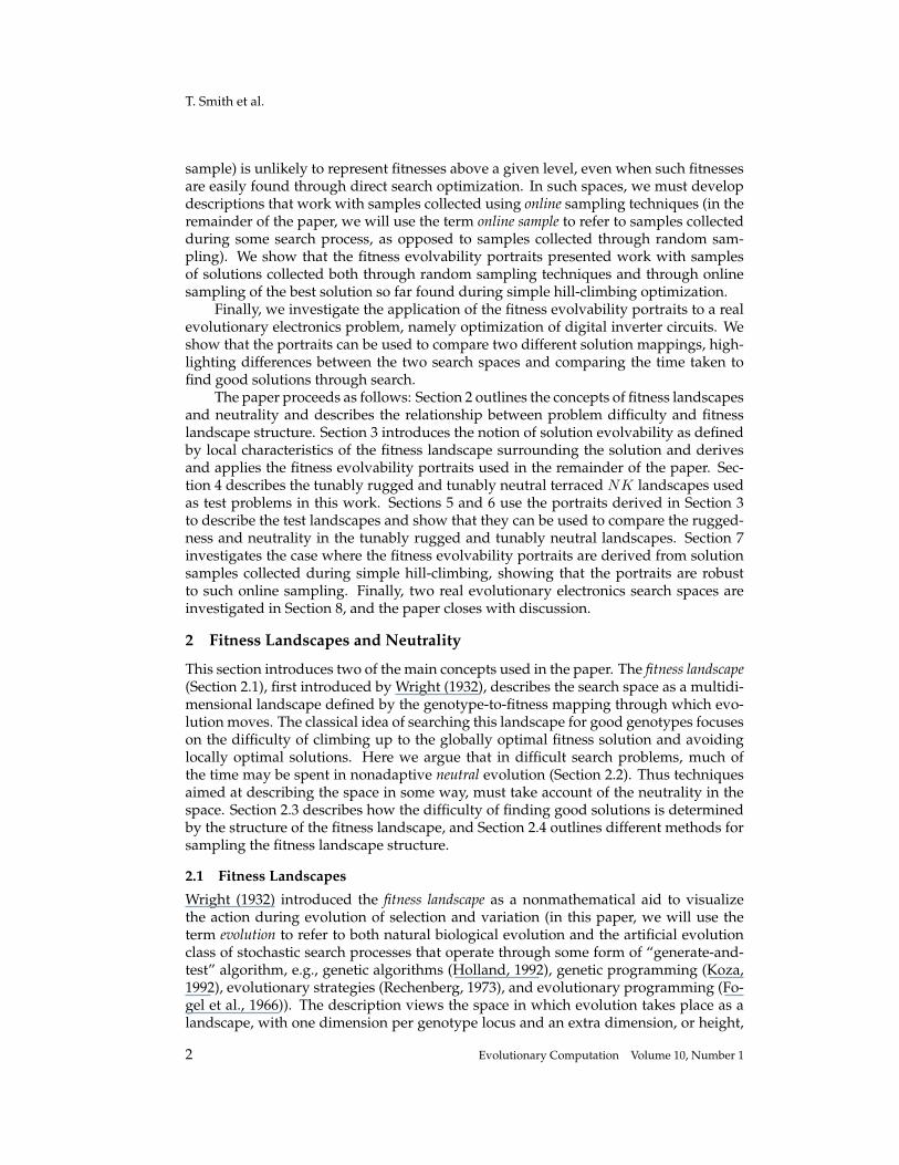
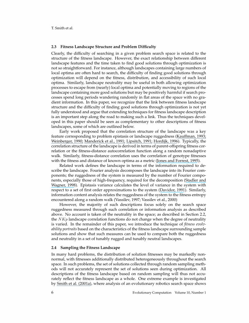
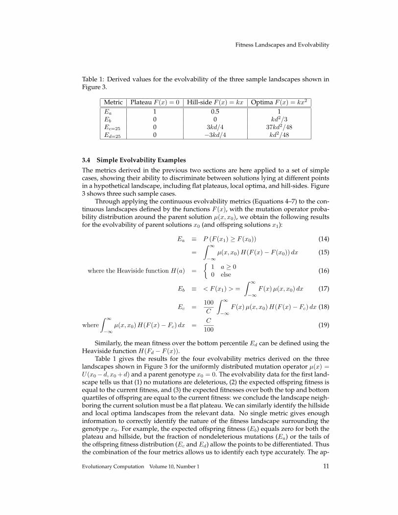
(a) Unconnected peaks (b) Single neutral pathway (c) Broad neutral plateau
Figure 2: Three two-dimensional model fitness landscapes showing the possible ad-vantage of neutrality in a simple landscape with one globally optimal and one (nearly)locally optimal peak. (a) shows the two peaks as unconnected; populations evolving tothe locally optimal peak will have difficulty moving to the global optimum. (b) showsthe two peaks connected by a single neutral pathway; a population on the suboptimalpeak may find the pathway. (c) shows the two peaks connected by a broad plateau; thepopulation will move easily from the suboptimal peak to the global optimum.
clearly exist in the graph, occurring as graph nodes from which all connected nodesare of lower fitness. This definition may produce local optima with respect to geneticoperators other than mutation; for example, some solutions may be local optima withrespect to recombination operators.
The graph definition of the search space highlights the dangers in the simple visu-alizable picture afforded to us by the fitness landscape description: our intuitive viewmay not apply in higher-dimensional spaces. Fisher, for example, argued that localoptima may not exist in a large class of high-dimensional spaces; the probability thata solution is optimal in every single dimension simultaneously is negligible (Provine,1986, 274). However, it should be stressed that many problems clearly do show localoptimality, e.g., the traveling salesman problem (Lawler et al., 1985). The next sectionintroduces the idea of search space neutrality, one possible way in which some high-dimension spaces may differ radically from our intuitive viewpoint.
2.2 Fitness Landscape Neutrality
In the neutral theory, it is argued that evolving populations may spend relatively largeperiods of time undergoing nonadaptive neutral mutation (Kimura, 1983), staying at aconstant height in the fitness landscape. The evolutionary timescale may be dominatedby long periods of neutral epochs (van Nimwegen et al., 1999) interspersed with shortperiods of rapid fitness increase, i.e., punctuated equilibrium (Eldredge and Gould, 1972;Gould and Eldredge, 1977; Elena et al., 1996). During these neutral epochs, the popu-lation will move in the space through random drift (note that this is a separate processto Wright’s idea of genetic drift due to finite population size (Provine, 1986)). Despitethe undirected nature of the population movement, neutrality can be of use in escapingfrom (nearly) locally optimal solutions: Figure 2 shows three model landscapes illus-trating the possible advantages of neutrality.
4 Evolutionary Computation Volume 10, Number 1
Fitness Landscapes and Evolvability
Neutral mutation in a fitness landscape will occur as movement between solutionsof equal fitness, i.e., movement along neutral networks. Such neutral evolution cannot bedistinguished from a population stuck in a local optimum simply through the fitness ofthe population over time. Instead, the underlying dynamics of the population must beinvestigated. Two key features have been predicted that distinguish the behavior of thepopulation during these periods of neutral drift from the behavior of a population stuckin a local optimum. The first key feature is movement, i.e., is the population movingsignificantly in genotype space. The second key feature is constant innovation, i.e., thenumber of previously unencountered phenotypes seen over time is constant. Thus anyphenotype should be accessible from a large enough neutral network; neutral drift caneventually find a higher fitness genotype and jump up to a higher neutral network.
These key features have been analyzed in many theoretical landscapes. Land-scapes produced by RNA secondary structure folding algorithms show that neutralwalks (a neutral variant on the random walk, where successive genotypes are gener-ated by application of the mutation operator) have the property of constant innovation(Huynen et al., 1996; Huynen, 1996). Exhaustive analysis of some RNA landscapeshas even mapped out the extent of the neutral networks and calculated the transitionprobabilities between the different networks (Forst et al., 1995; Gruner et al., 1996).Barnett (1998) introduces the NKp landscape, a tunably neutral variant on Kauffman’sNK systems (Kauffman, 1993), and through calculation of population diffusion coef-ficients, shows highly neutral landscapes produce much more population movementduring periods of no fitness change when compared to such periods in landscapes ofzero neutrality. An important result from the NKp landscape work is that changingthe amount of neutrality in the landscape has no effect on the ruggedness correlationfunction; correlation lengths do not predict the change in evolutionary dynamics seenfor NKp landscapes of different neutrality (Barnett, 1998). Newman and Engelhardt(1998) investigate a similar tunably neutral variant of the NK system, finding that in-creased neutrality allows high fitness solutions to be found more easily through search.This is supported by Shackleton et al. (2000) who find that adding neutrality throughredundancy can improve the level of fitness found through artificial evolution.
Neutrality has also been shown in real-world problem landscapes: In experimentson evolving tone recognition circuits, populations were seen to move in genotype spaceduring periods where fitness did not increase (Harvey and Thompson, 1996). Exper-iments on evolution of digital circuits under two conditions – allowing neutral muta-tions and not allowing such changes – have also shown the importance of neutrality tothe search process. Experiments where neutral changes were allowed consistently pro-duced two-bit multiplier solutions of higher fitness than experiments without neutralmutation (Vassilev and Miller, 2000). Also, Thompson (2001) reports on the presence ofneutral plateaus in evolving speech recognition circuits and shows through exhaustivemutation of genotypes at the start of the plateau that no transitions exist to a higherfitness level; the neutral evolution phase is necessary.
The degree of neutrality in a system is clearly a factor in the population dynamicsduring evolution. However, many fitness landscape descriptions simply do not iden-tify this factor, e.g., the work on NKp landscapes showing that the autocorrelationfunction does not change with the level of neutrality (Barnett, 1998). In the next sec-tion, we describe the relationship between the structure of the fitness landscape and thedifficulty of searching in the landscape, and we outline methods by which the fitnesslandscape is typically described.
Evolutionary Computation Volume 10, Number 1 5
T. Smith et al.
2.3 Fitness Landscape Structure and Problem Difficulty
Clearly, the difficulty of searching in a given problem search space is related to thestructure of the fitness landscape. However, the exact relationship between differentlandscape features and the time taken to find good solutions through optimization isnot so straightforward. For instance, although landscapes containing large numbers oflocal optima are often hard to search, the difficulty of finding good solutions throughoptimization will depend on the fitness, distribution, and accessibility of such localoptima. Similarly, landscape neutrality may be useful in both allowing optimizationprocesses to escape from (nearly) local optima and potentially moving to regions of thelandscape containing more good solutions but may be positively harmful if search pro-cesses spend long periods wandering randomly in flat areas of the space with no gra-dient information. In this paper, we recognize that the link between fitness landscapestructure and the difficulty of finding good solutions through optimization is not yetfully understood and argue that extending techniques for fitness landscape descriptionis an important step along the road to making such a link. Thus the techniques devel-oped in this paper should be seen as complementary to other descriptions of fitnesslandscapes, some of which are outlined below.
Early work proposed that the correlation structure of the landscape was a keyfeature corresponding to problem epistasis or landscape ruggedness (Kauffman, 1993;Weinberger, 1990; Manderick et al., 1991; Lipsitch, 1991; Hordijk, 1996). Typically, thecorrelation structure of the landscape is derived in terms of parent-offspring fitness cor-relation or the fitness-distance autocorrelation function along a random nonadaptivewalk. Similarly, fitness-distance correlation uses the correlation of genotype fitnesseswith the fitness and distance of known optima as a metric (Jones and Forrest, 1995).
Related work defines the landscape in terms of the information required to de-scribe the landscape. Fourier analysis decomposes the landscape into its Fourier com-ponents; the ruggedness of the system is measured by the number of Fourier compo-nents, especially those of high-frequency, required for the decomposition (Stadler andWagner, 1998). Epistasis variance calculates the level of variance in the system withrespect to a set of first order approximations to the system (Davidor, 1991). Similarly,information content analysis relates the ruggedness of the system to the fitness entropyencountered along a random walk (Vassilev, 1997; Vassilev et al., 2000)
However, the majority of such descriptions focus solely on the search spaceruggedness measured through such correlation or information analysis as describedabove. No account is taken of the neutrality in the space; as described in Section 2.2,the NKp landscape correlation functions do not change when the degree of neutralityis varied. In the remainder of this paper, we introduce the technique of fitness evolv-ability portraits based on the characteristics of the fitness landscape surrounding samplesolutions and show that such measures can be used to compare both the ruggednessand neutrality in a set of tunably rugged and tunably neutral landscapes.
2.4 Sampling the Fitness Landscape
In many hard problems, the distribution of solution fitnesses may be markedly non-normal, with fitnesses additionally distributed heterogeneously throughout the searchspace. In such problems, the set of solutions collected through random sampling meth-ods will not accurately represent the set of solutions seen during optimization. Alldescriptions of the fitness landscape based on random sampling will thus not accu-rately reflect the fitness landscape as a whole. One extreme example is investigatedby Smith et al. (2001a), where analysis of an evolutionary robotics search space shows
6 Evolutionary Computation Volume 10, Number 1
Fitness Landscapes and Evolvability
that fewer than 0.0001% of solutions in a random sample have fitness above 50% ofthe maximum in a neural network robot control problem despite this fitness being rela-tively easy to reach using optimization techniques. Two spaces that differ only in highfitness regions may show markedly different times to find good solutions through opti-mization, but fitness landscape descriptions based on random sampling will not showthese differences (Smith et al., 2001a)
One potential approach is to bias the random sample procedure, keeping onlysome set percentage of solutions at each fitness. Even this method may fail to collectsolutions above some fitness level in reasonable time, and it may be necessary to per-form some kind of directed search process to collect the sample. Clearly, there is somepoint at which the time taken to collect such a sample may well approach a significantfraction of the time taken to solve the problem. For instance, if the sample required tocharacterize the problem involves collecting solutions at or near the optimum, we willhave effectively solved the problem merely in the act of description. A useful analogycould be drawn with Marr’s type II systems; the system may not be reducible to a sim-pler level of description than the system itself (Marr, 1976). By contrast, type I systemscan be reduced to a simpler description, e.g., a fitness landscape that can usefully bereduced to a single correlation length description.
In Section 7, we collect samples though simple hill-climbing, and show that thefitness evolvability portraits based on the biased sample set make the same predictionsas those based on unbiased random samples. Although the NK landscapes used in thispaper have approximately normal fitness distributions, verifying that the portraits arereasonably robust to sample bias is important if we are to use them on other problemswith highly skewed fitness distributions (Smith et al., 2001b).
In the next section, we introduce the notion of evolvability as the capacity of asolution to evolve, closely tied to the fitness landscape neighboring that solution. Wethen derive a set of solution and population evolvability metrics using them to buildfitness evolvability portraits of sample fitness landscapes.
3 Evolvability and the Transmission Function
Evolvability is loosely defined as the capacity to evolve, alternatively the ability of anindividual or population to generate fit variants (Altenberg, 1994; Marrow, 1999; Wag-ner and Altenberg, 1996). Thus evolvability is more closely allied with the potential forfitness than with fitness itself; two equal fitness individuals or populations can havevery different evolvabilities (Turney, 1999). Typically, researchers use some definitionof evolvability based on the offspring of current individuals or populations: in thispaper we follow Cavalli-Sforza and Feldman (1976) and Altenberg (1994) in using thetransmission function of all possible offspring from a parent to define a set of metrics ofevolvability (see Section 3.1 for further details).
It is often argued that there may be long-term trends for evolvability to increaseduring evolution (see Wilke (2001) and Turney (1999)). However, as evolvability ismore directly related to fitness potential than fitness itself, long-term change cannot bedue to straight fitness selection. Thus any trend towards change in evolvability can onlybe understood through some second order selection mechanism by which evolutiontends to retain solutions that have a more evolvable genetic system (Dawkins, 1989;Kirschner and Gerhart, 1998).
Researchers in both biology and evolutionary computation typically link evolv-ability with the local structure of the search space. For example, Burch and Chao (2000)show that RNA virus evolvability can be understood in terms of the mutational neigh-
Evolutionary Computation Volume 10, Number 1 7
T. Smith et al.
borhood, while many evolutionary computation researchers (see Ebner et al. (2001) andMarrow (1999)) argue that changing the properties of the search space (through suchmechanisms as adding neutrality) can affect evolvability as evidenced by the speed ofevolution. The interest in evolvability for evolutionary computation practitioners isthus tied closely to work on the ruggedness and modality of the search space, arguedto primarily influence the ease of finding good solutions in the space (Weinberger, 1990;Hordijk, 1996; Jones and Forrest, 1995; Naudts and Kallel, 2000).
Recent work has emphasized that in addition to landscape ruggedness and modal-ity, search space neutrality may have impact on the population dynamics of evolution(Section 2.2). This factor may not be identified by many standard measures aimed atthe landscape ruggedness and local modality but may be measurable through changein evolvability. For example, recent artificial evolution research has shown that evolv-ability can change during neutral epochs; populations tend to move to “flatter” areas ofthe fitness landscape where fewer mutations are deleterious (Wilke et al., 2001; Wilke,2001). This can clearly have an impact on the speed of search but may not be picked upby the standard landscape ruggedness and modality descriptions.
Other biological research in evolvability is also relevant to evolutionary computa-tion, e.g., the work on adaptation to change in environment through such mechanismsas alleles providing increased mutation rates (Taddei et al., 1997; Sniegowski et al.,1997). However, in this paper we focus on evolvability in terms of the properties ofthe solutions’ local search space. The next section outlines the offspring transmissionfunction and defines a simple set of evolvability metrics.
3.1 The Transmission Function
In this paper, we follow the definition of evolvability as the ability of individuals andpopulations to produce fit variants, specifically the ability to both produce fitter vari-ants and to not produce less fit variants. This definition is intimately tied in with re-search on the transmission function T (Altenberg, 1994; Cavalli-Sforza and Feldman,1976) and the population offspring probability distribution function φ from all possibleapplications of the genetic operators to the parent(s)
φ(g, f) =∫ ∫ ∫ ∫
ψ(h, k, h′, k′)T (g, f : h, k, h′, k′) dh dk dh′ dk′ (1)
or the probability φ (with parental selection function ψ) of obtaining offspring genotypeg and phenotype f over all parents of genotypes h, h′ and phenotypes k, k′. The trans-mission function T is the probability density function of obtaining g, f given h, k, h′, k′
(Cavalli-Sforza and Feldman, 1976).In the absence of recombination, only a single parent h, k is required to produce
offspring through mutation (in Section 9 we discuss the impact of recombination onthe techniques developed in this paper):
φ(g, f) =∫ ∞
−∞ψ(h, k) T (g, f : h, k) dh dk (2)
or the probability of obtaining offspring g, f over all parents h, k with selection ψ. Inthis paper, we focus on the offspring of a set of single genotypes (saved during thecourse of evolutionary runs), so do not integrate over the set of all possible parents.Similarly, the selection function can be omitted as we preselect the parent. Since we areinterested only in the offspring phenotypes f and not the offspring genotypes g, we can
8 Evolutionary Computation Volume 10, Number 1
Fitness Landscapes and Evolvability
refer to the transmission function T (f : h, k) as shorthand for the probability densityfunction of offspring fitnesses from a single parent h, k.
The transmission function thus encompasses both the operators and the represen-tation; instead of referring to good and bad genetic operators or good and bad repre-sentations, we can talk about the effectiveness of the transmission function. Thus theevolvability of an individual or population, i.e., their ability to generate fit variants,is simply a property of the individual or population transmission function. The nextsection derives measures for the evolvability of an individual solution in terms of thistransmission function for continuous variables.
3.2 Evolvability Metrics: Continuous Variables
The evolvability of a solution genotype h and fitness k is directly tied to the probabilityof that solution not producing offspring of lower fitness. Thus we derive our first metricof evolvability Ea:
Ea =
∫∞k
T (f : h, k) df∫∞−∞ T (f : h, k) df
(3)
or the probability that the offspring fitness f is greater or equal to the current fitnessk, i.e., the mutation is nondeleterious. Since the transmission function T (f : h, k) is aprobability density function, the infinite integral sums to unity, so we have
Ea =∫ ∞
k
T (f : h, k) df (4)
Low fitness solutions may have a larger Ea than high fitness solutions simply dueto the increased number of better mutations. The second evolvability metric Eb usesonly the offspring fitnesses:
Eb =∫ ∞
−∞f T (f : h, k) df (5)
or the expected offspring fitness from genotype h. Note, this value is fitness dependentso should not be compared across genotypes without reference to their original fitness.A further problem with both Ea and Eb is their dependence on the entire set of offspringfitnesses; the fraction of offspring that are significantly fitter than the parent may beextremely small. The third measure reflects this dimension of evolvability, looking onlyat the top Cth percentile of the offspring fitnesses
Ec =100C
∫ ∞
Fc
f T (f : h, k) df (6)
where Fc defined by∫ ∞
Fc
T (f : h, k) df =C
100(7)
or the expected fitness of only the top Cth percentile of fitnesses. A similar measure Ed
(not shown) calculates the expected fitness of the bottom Cth percentile of offspring.The next section extends the continuous analysis presented above to the discrete
set.
3.3 Evolvability Metrics: The Discrete Set
Consider the fitness landscape as a directed graph (V, E) with vertices V (genotypes)connected by edges E (defined by the genetic operators). The set G of offspring from a
Evolutionary Computation Volume 10, Number 1 9

T. Smith et al.
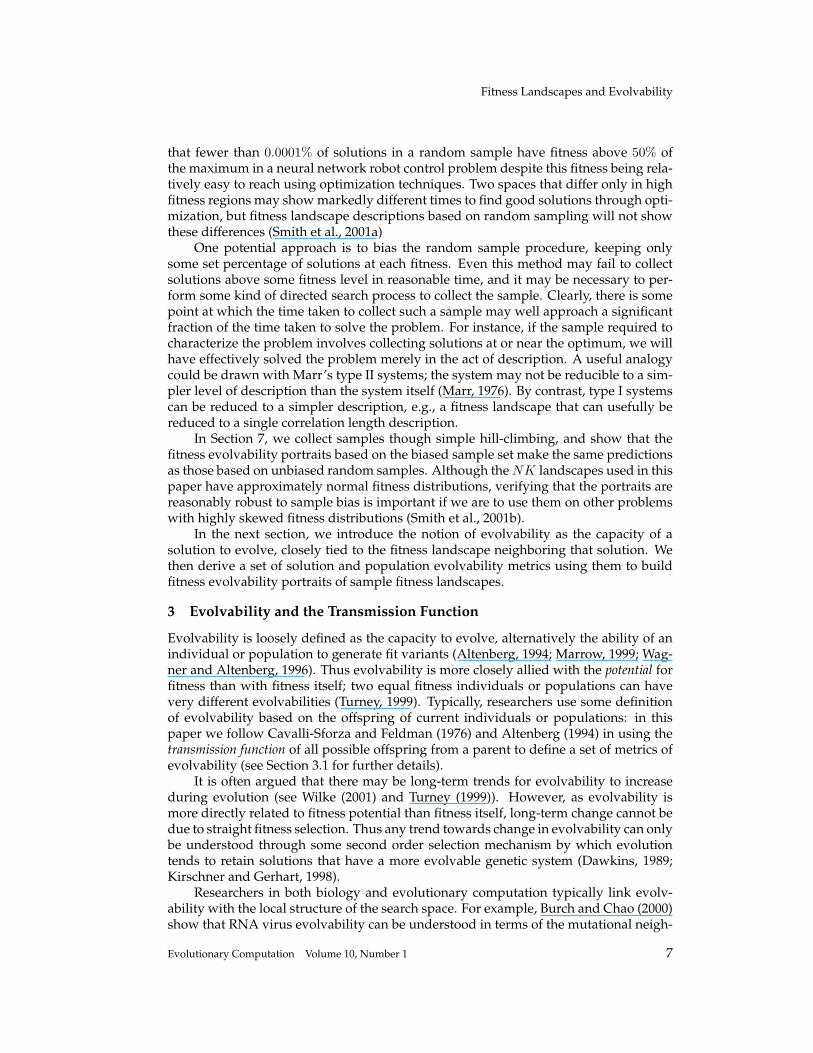
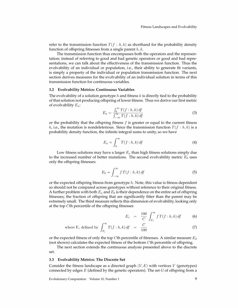
(a) F (x) = 0 (b) F (x) = kx (c) F (x) = kx2
Figure 3: Three continuous one-dimensional landscapes F (x) with the parent genotypex0 shown by the solid circle lying at x = 0 (in all cases, F (0) = 0). The mutationoperator µ(x, x0) is a probability distribution function, producing offspring x1 lyingin a uniform distribution around x with range d, shown by the thick bar below eachlandscape, centered on x0. See text for the derived evolvability in each landscape.
parent genotype h, k is thus defined by the vertices connected to the parent vertex:
G(h, k) = {g ∈ V : E(h, k) = g} (8)
The fitness function F maps each vertex on to a single fitness, so similarly, wedefine the set of offspring with fitness F (g) equal to or greater than some fitness c:
G+c (h, k) = {g ∈ V : E(h, k) = g, F (g) ≥ c} (9)
The probability of the offspring fitness being higher or equal to the parent fitness,or Ea, is simply the fraction of the set with F (g) ≥ k:
Ea =|G+
k (h, k)||G(h, k)| (10)
As in the previous section, the mean fitness of the offspring solutions, or Eb, issimply the mean fitness of all members of the set:
Eb =
∑g∈G(h,k) F (g)
|G(h, k)| (11)
The mean fitness of the set of offspring with fitness in the top Cth percentile issimilarly defined:
Ec =
∑g∈G+
Fc(h,k) F (g)
|G+Fc
(h, k)| (12)
where Fc defined by |G+Fc
(h, k)| =C |G(h, k)|
100(13)
The mean fitness of the set of offspring with fitness in the bottom percentile can bedefined through the set G−Fd
(h, k) of offspring with fitness below some fitness Fd.The next section applies the metrics to a set of simple cases, where the parent geno-
types lie at different points in a hypothetical landscape.
10 Evolutionary Computation Volume 10, Number 1
Fitness Landscapes and Evolvability
Table 1: Derived values for the evolvability of the three sample landscapes shown inFigure 3.
Metric Plateau F (x) = 0 Hill-side F (x) = kx Optima F (x) = kx2
Ea 1 0.5 1Eb 0 0 kd2/3Ec=25 0 3kd/4 37kd2/48Ed=25 0 −3kd/4 kd2/48
3.4 Simple Evolvability Examples
The metrics derived in the previous two sections are here applied to a set of simplecases, showing their ability to discriminate between solutions lying at different pointsin a hypothetical landscape, including flat plateaus, local optima, and hill-sides. Figure3 shows three such sample cases.
Through applying the continuous evolvability metrics (Equations 4–7) to the con-tinuous landscapes defined by the functions F (x), with the mutation operator proba-bility distribution around the parent solution µ(x, x0), we obtain the following resultsfor the evolvability of parent solutions x0 (and offspring solutions x1):
Ea ≡ P (F (x1) ≥ F (x0)) (14)
=∫ ∞
−∞µ(x, x0) H(F (x)− F (x0)) dx (15)
where the Heaviside function H(a) ={
1 a ≥ 00 else (16)
Eb ≡ < F (x1) > =∫ ∞
−∞F (x) µ(x, x0) dx (17)
Ec =100C
∫ ∞
−∞F (x) µ(x, x0) H(F (x)− Fc) dx (18)
where∫ ∞
−∞µ(x, x0)H(F (x)− Fc) dx =
C
100(19)
Similarly, the mean fitness over the bottom percentile Ed can be defined using theHeaviside function H(Fd − F (x)).
Table 1 gives the results for the four evolvability metrics derived on the threelandscapes shown in Figure 3 for the uniformly distributed mutation operator µ(x) =U(x0− d, x0 + d) and a parent genotype x0 = 0. The evolvability data for the first land-scape tells us that (1) no mutations are deleterious, (2) the expected offspring fitness isequal to the current fitness, and (3) the expected fitnesses over both the top and bottomquartiles of offspring are equal to the current fitness: we conclude the landscape neigh-boring the current solution must be a flat plateau. We can similarly identify the hillsideand local optima landscapes from the relevant data. No single metric gives enoughinformation to correctly identify the nature of the fitness landscape surrounding thegenotype x0. For example, the expected offspring fitness (Eb) equals zero for both theplateau and hillside, but the fraction of nondeleterious mutations (Ea) or the tails ofthe offspring fitness distribution (Ec and Ed) allow the points to be differentiated. Thusthe combination of the four metrics allows us to identify each type accurately. The ap-
Evolutionary Computation Volume 10, Number 1 11
T. Smith et al.
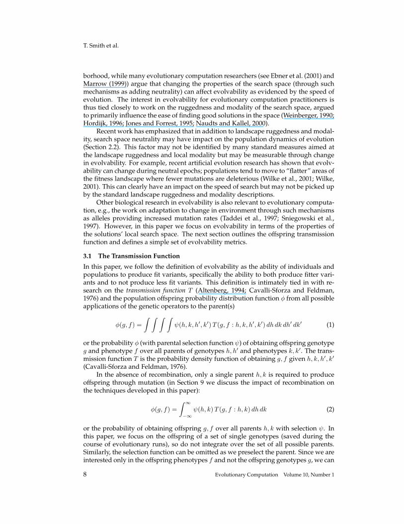
(a) Unconnected peaks (b) Single neutral pathway (c) Broad neutral plateau
Figure 4: Three two-dimensional model fitness landscapes showing the possible ad-vantage of neutrality in a simple landscape with one globally optimal and one (nearly)locally-optimal deceptive peak. The two peaks have fitnesses of 1.0 and 0.5, respec-tively, and the neutral pathway and plateau have fitnesses of 0.5.
proach can also be used on problems with higher dimensional landscapes, although theoffspring distributions may need to be approximated through sampled applications ofthe mutation operator(s).
In the next section, we show how these evolvability metrics can be averaged overpopulations of solutions to produce the fitness evolvability portraits used in the re-mainder of this paper, and relate these portraits to levels of ruggedness, modality, andneutrality in the landscape.
3.5 Population Fitness Evolvability Portraits
The previous section described how the evolvability metrics could be calculated overthe fitness neighborhood for a single solution genotype. We can define the same evolv-ability metrics over a sampled population of solutions through simply defining themetrics as calculated over the sum of population transmission functions, i.e., we takethe distribution of offspring fitnesses from all members of the sample and calculatethe evolvability metrics. For the discrete case, this translates to taking the populationset of offspring defined over the combined sets of offspring from all members of thepopulation.
Two important ideas emerge from this definition of population evolvability. First,we can compare entire populations simply by comparing their metrics of evolvability.This is not explored further in this paper but has been used by Smith et al. (2001c, 2001d)to investigate the behavior of populations during neutral epochs, in particular whetherthe populations are moving to more evolvable areas of space during such neutralepochs. Second, we can take samples of equal fitness (in practice, we take samplesof nearly equal fitness lying in some range) to build up a fitness evolvability portrait ofthe landscape. For each equal fitness sample of solutions, we can calculate the popula-tion evolvability and plot the evolvability metrics against solution fitness2.
2It should be noted that the idea of plotting some measure over fitness was used by Rose et al. (1996) intheir density of states approach. However, in this paper, we focus on the evolvability of solutions at somefitness rather than simply the number of such solutions.
12 Evolutionary Computation Volume 10, Number 1
Fitness Landscapes and Evolvability
0 0.2 0.4 0.6 0.8 120
30
40
50
60
70
80
90
100
Original Fitness
Pro
b(F
mut
≥ F
curr
ent)
Unconnected Neutral pathwayNeutral plateau
(a) Probability of a nondeleterious mutation Ea
0 0.2 0.4 0.6 0.8 10
0.1
0.2
0.3
0.4
0.5
0.6
0.7
0.8
0.9
1
Original Fitness
< F
0,10
0 >
Unconnected Neutral pathwayNeutral plateau
(b) Expected fitness over all mutations Eb
0 0.2 0.4 0.6 0.8 10
0.1
0.2
0.3
0.4
0.5
0.6
0.7
0.8
0.9
1
Original Fitness
< F
75,1
00 >
Unconnected Neutral pathwayNeutral plateau
(c) Expected fitness over top quartile of muta-tions Ec
0 0.2 0.4 0.6 0.8 10
0.1
0.2
0.3
0.4
0.5
0.6
0.7
0.8
0.9
1
Original Fitness
< F
0,25
>Unconnected Neutral pathwayNeutral plateau
(d) Expected fitness over bottom quartile of mu-tations Ed
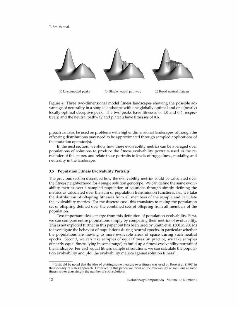
Figure 5: Fitness evolvability portraits for the three model landscapes shown in Figure4. The evolvability metrics were calculated from an exhaustive sample set of solutions.
3.5.1 Three Model Landscapes
In this section, we show how the fitness evolvability portraits can be derived for thethree model landscapes shown in Figure 4 and illustrate the advantages of the portraitsover other available landscape descriptions.
Figure 4 shows the same three model landscapes used in Section 2.2 to illustratethe potential advantages of landscape neutrality. It should be emphasized that thelandscapes are used purely to illustrate the potential advantage for searching in land-scapes with varying levels of neutrality and are not drawn from real problem spaces.The three landscapes shown here are discrete-valued 100-by-100 grids, and for both theadaptive walks and the evolvability analysis on these landscapes, the same mutationoperator was used whereby offspring solutions were created from any one of the eightgrid nearest neighbors.
Evolutionary Computation Volume 10, Number 1 13
T. Smith et al.
0.3 0.35 0.4 0.45 0.5 0.55 0.620
30
40
50
60
70
80
90
100
Original Fitness
Pro
b(F
mut
≥ F
curr
ent)
Unconnected Neutral pathwayNeutral plateau
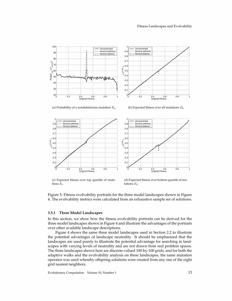
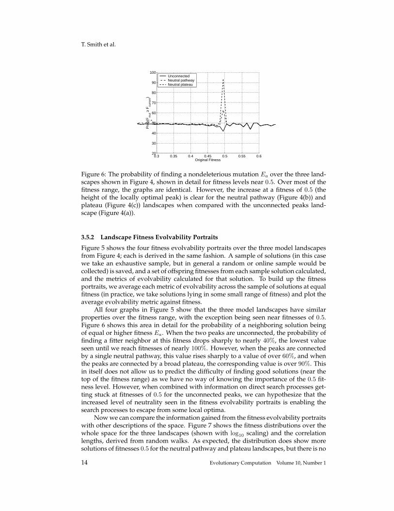
Figure 6: The probability of finding a nondeleterious mutation Ea over the three land-scapes shown in Figure 4, shown in detail for fitness levels near 0.5. Over most of thefitness range, the graphs are identical. However, the increase at a fitness of 0.5 (theheight of the locally optimal peak) is clear for the neutral pathway (Figure 4(b)) andplateau (Figure 4(c)) landscapes when compared with the unconnected peaks land-scape (Figure 4(a)).
3.5.2 Landscape Fitness Evolvability Portraits
Figure 5 shows the four fitness evolvability portraits over the three model landscapesfrom Figure 4; each is derived in the same fashion. A sample of solutions (in this casewe take an exhaustive sample, but in general a random or online sample would becollected) is saved, and a set of offspring fitnesses from each sample solution calculated,and the metrics of evolvability calculated for that solution. To build up the fitnessportraits, we average each metric of evolvability across the sample of solutions at equalfitness (in practice, we take solutions lying in some small range of fitness) and plot theaverage evolvability metric against fitness.
All four graphs in Figure 5 show that the three model landscapes have similarproperties over the fitness range, with the exception being seen near fitnesses of 0.5.Figure 6 shows this area in detail for the probability of a neighboring solution beingof equal or higher fitness Ea. When the two peaks are unconnected, the probability offinding a fitter neighbor at this fitness drops sharply to nearly 40%, the lowest valueseen until we reach fitnesses of nearly 100%. However, when the peaks are connectedby a single neutral pathway, this value rises sharply to a value of over 60%, and whenthe peaks are connected by a broad plateau, the corresponding value is over 90%. Thisin itself does not allow us to predict the difficulty of finding good solutions (near thetop of the fitness range) as we have no way of knowing the importance of the 0.5 fit-ness level. However, when combined with information on direct search processes get-ting stuck at fitnesses of 0.5 for the unconnected peaks, we can hypothesize that theincreased level of neutrality seen in the fitness evolvability portraits is enabling thesearch processes to escape from some local optima.
Now we can compare the information gained from the fitness evolvability portraitswith other descriptions of the space. Figure 7 shows the fitness distributions over thewhole space for the three landscapes (shown with log10 scaling) and the correlationlengths, derived from random walks. As expected, the distribution does show moresolutions of fitnesses 0.5 for the neutral pathway and plateau landscapes, but there is no
14 Evolutionary Computation Volume 10, Number 1
Fitness Landscapes and Evolvability
0 0.25 0.5 0.75 110
-4
10-3
10-2
10-1
100
�
fitness
frac
tion
UnconnectedPathway Plateau
(a) Fitness distribution
Unconnected Pathway Plateau0
2
4
6
8
10
12
Cor
rela
tion
leng
th, ρ
(b) Correlation lengths
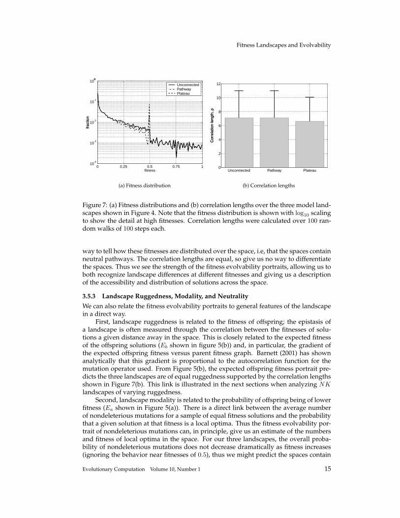
Figure 7: (a) Fitness distributions and (b) correlation lengths over the three model land-scapes shown in Figure 4. Note that the fitness distribution is shown with log10 scalingto show the detail at high fitnesses. Correlation lengths were calculated over 100 ran-dom walks of 100 steps each.
way to tell how these fitnesses are distributed over the space, i.e, that the spaces containneutral pathways. The correlation lengths are equal, so give us no way to differentiatethe spaces. Thus we see the strength of the fitness evolvability portraits, allowing us toboth recognize landscape differences at different fitnesses and giving us a descriptionof the accessibility and distribution of solutions across the space.
3.5.3 Landscape Ruggedness, Modality, and NeutralityWe can also relate the fitness evolvability portraits to general features of the landscapein a direct way.
First, landscape ruggedness is related to the fitness of offspring; the epistasis ofa landscape is often measured through the correlation between the fitnesses of solu-tions a given distance away in the space. This is closely related to the expected fitnessof the offspring solutions (Eb shown in figure 5(b)) and, in particular, the gradient ofthe expected offspring fitness versus parent fitness graph. Barnett (2001) has shownanalytically that this gradient is proportional to the autocorrelation function for themutation operator used. From Figure 5(b), the expected offspring fitness portrait pre-dicts the three landscapes are of equal ruggedness supported by the correlation lengthsshown in Figure 7(b). This link is illustrated in the next sections when analyzing NKlandscapes of varying ruggedness.
Second, landscape modality is related to the probability of offspring being of lowerfitness (Ea shown in Figure 5(a)). There is a direct link between the average numberof nondeleterious mutations for a sample of equal fitness solutions and the probabilitythat a given solution at that fitness is a local optima. Thus the fitness evolvability por-trait of nondeleterious mutations can, in principle, give us an estimate of the numbersand fitness of local optima in the space. For our three landscapes, the overall proba-bility of nondeleterious mutations does not decrease dramatically as fitness increases(ignoring the behavior near fitnesses of 0.5), thus we might predict the spaces contain
Evolutionary Computation Volume 10, Number 1 15
T. Smith et al.
K=0 K=1 K=2 K=6 K=12 K=18 K=240
1
2
3
4
5
6
7
8
9
10
Mea
n C
orre
latio
n Le
ngth
[NK
P: N
=25
, F=∞
]
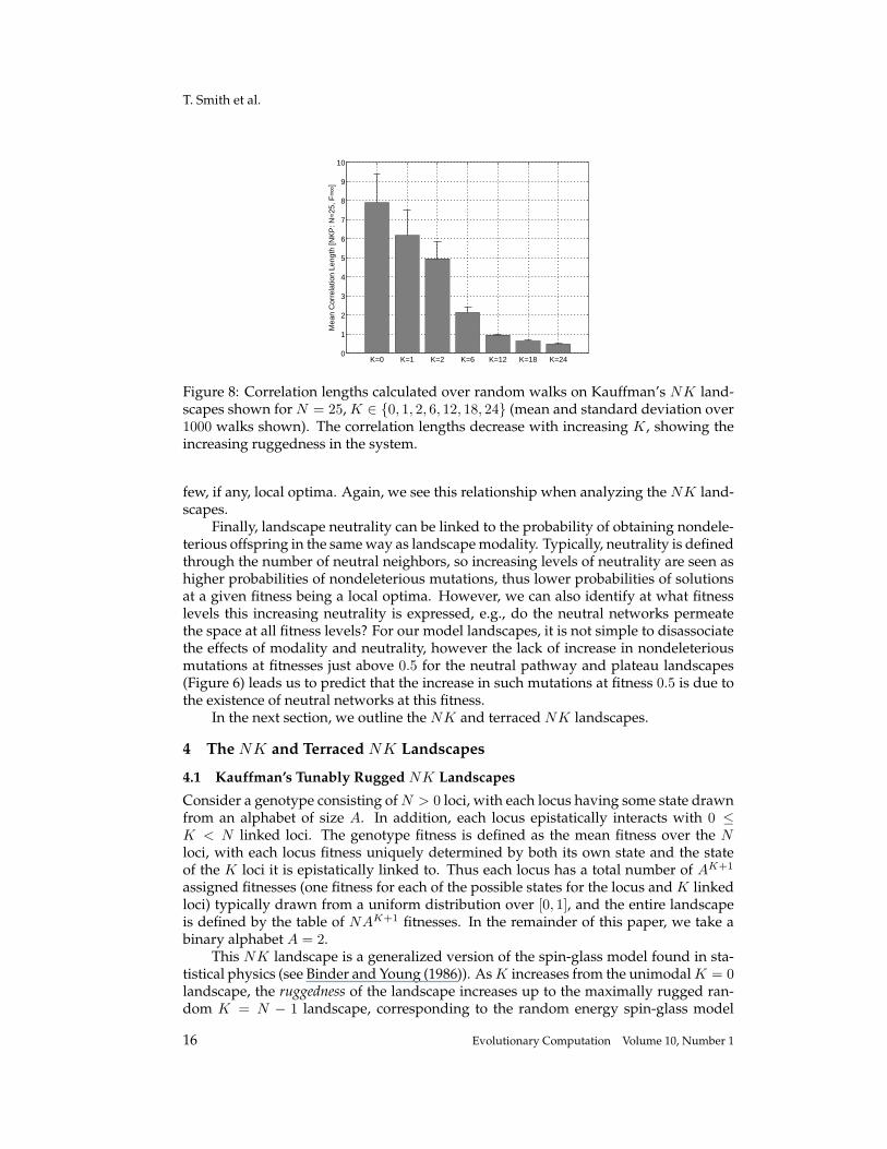
Figure 8: Correlation lengths calculated over random walks on Kauffman’s NK land-scapes shown for N = 25, K ∈ {0, 1, 2, 6, 12, 18, 24} (mean and standard deviation over1000 walks shown). The correlation lengths decrease with increasing K, showing theincreasing ruggedness in the system.
few, if any, local optima. Again, we see this relationship when analyzing the NK land-scapes.
Finally, landscape neutrality can be linked to the probability of obtaining nondele-terious offspring in the same way as landscape modality. Typically, neutrality is definedthrough the number of neutral neighbors, so increasing levels of neutrality are seen ashigher probabilities of nondeleterious mutations, thus lower probabilities of solutionsat a given fitness being a local optima. However, we can also identify at what fitnesslevels this increasing neutrality is expressed, e.g., do the neutral networks permeatethe space at all fitness levels? For our model landscapes, it is not simple to disassociatethe effects of modality and neutrality, however the lack of increase in nondeleteriousmutations at fitnesses just above 0.5 for the neutral pathway and plateau landscapes(Figure 6) leads us to predict that the increase in such mutations at fitness 0.5 is due tothe existence of neutral networks at this fitness.
In the next section, we outline the NK and terraced NK landscapes.
4 The NK and Terraced NK Landscapes
4.1 Kauffman’s Tunably Rugged NK Landscapes
Consider a genotype consisting of N > 0 loci, with each locus having some state drawnfrom an alphabet of size A. In addition, each locus epistatically interacts with 0 ≤K < N linked loci. The genotype fitness is defined as the mean fitness over the Nloci, with each locus fitness uniquely determined by both its own state and the stateof the K loci it is epistatically linked to. Thus each locus has a total number of AK+1
assigned fitnesses (one fitness for each of the possible states for the locus and K linkedloci) typically drawn from a uniform distribution over [0, 1], and the entire landscapeis defined by the table of NAK+1 fitnesses. In the remainder of this paper, we take abinary alphabet A = 2.
This NK landscape is a generalized version of the spin-glass model found in sta-tistical physics (see Binder and Young (1986)). As K increases from the unimodal K = 0landscape, the ruggedness of the landscape increases up to the maximally rugged ran-dom K = N − 1 landscape, corresponding to the random energy spin-glass model
16 Evolutionary Computation Volume 10, Number 1
Fitness Landscapes and Evolvability
K=0 K=1 K=2 K=6 K=12 K=18 K=240
1
2
3
4
5
6
7
8
9
10
Mea
n C
orre
latio
n Le
ngth
[NK
P: N
=25
, F=
4]
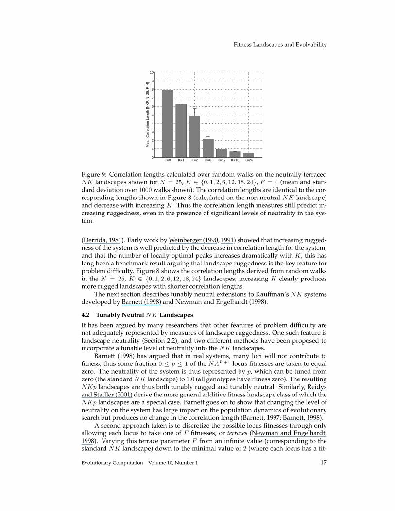
Figure 9: Correlation lengths calculated over random walks on the neutrally terracedNK landscapes shown for N = 25, K ∈ {0, 1, 2, 6, 12, 18, 24}, F = 4 (mean and stan-dard deviation over 1000 walks shown). The correlation lengths are identical to the cor-responding lengths shown in Figure 8 (calculated on the non-neutral NK landscape)and decrease with increasing K. Thus the correlation length measures still predict in-creasing ruggedness, even in the presence of significant levels of neutrality in the sys-tem.
(Derrida, 1981). Early work by Weinberger (1990, 1991) showed that increasing rugged-ness of the system is well predicted by the decrease in correlation length for the system,and that the number of locally optimal peaks increases dramatically with K; this haslong been a benchmark result arguing that landscape ruggedness is the key feature forproblem difficulty. Figure 8 shows the correlation lengths derived from random walksin the N = 25, K ∈ {0, 1, 2, 6, 12, 18, 24} landscapes; increasing K clearly producesmore rugged landscapes with shorter correlation lengths.
The next section describes tunably neutral extensions to Kauffman’s NK systemsdeveloped by Barnett (1998) and Newman and Engelhardt (1998).
4.2 Tunably Neutral NK Landscapes
It has been argued by many researchers that other features of problem difficulty arenot adequately represented by measures of landscape ruggedness. One such feature islandscape neutrality (Section 2.2), and two different methods have been proposed toincorporate a tunable level of neutrality into the NK landscapes.
Barnett (1998) has argued that in real systems, many loci will not contribute tofitness, thus some fraction 0 ≤ p ≤ 1 of the NAK+1 locus fitnesses are taken to equalzero. The neutrality of the system is thus represented by p, which can be tuned fromzero (the standard NK landscape) to 1.0 (all genotypes have fitness zero). The resultingNKp landscapes are thus both tunably rugged and tunably neutral. Similarly, Reidysand Stadler (2001) derive the more general additive fitness landscape class of which theNKp landscapes are a special case. Barnett goes on to show that changing the level ofneutrality on the system has large impact on the population dynamics of evolutionarysearch but produces no change in the correlation length (Barnett, 1997; Barnett, 1998).
A second approach taken is to discretize the possible locus fitnesses through onlyallowing each locus to take one of F fitnesses, or terraces (Newman and Engelhardt,1998). Varying this terrace parameter F from an infinite value (corresponding to thestandard NK landscape) down to the minimal value of 2 (where each locus has a fit-
Evolutionary Computation Volume 10, Number 1 17
T. Smith et al.
F=inf F=11 F=6 F=5 F=4 F=3 F=20
2
4
6
8
10
12
Mea
n C
orre
latio
n Le
ngth
[NK
P: N
=25
, K=
0]
(a) Terraced NK landscape, K = 0
F=inf F=11 F=6 F=5 F=4 F=3 F=20
0.2
0.4
0.6
0.8
1
1.2
1.4
Mea
n C
orre
latio
n Le
ngth
[NK
P: N
=25
, K=
12]
(b) Terraced NK landscape, K = 12
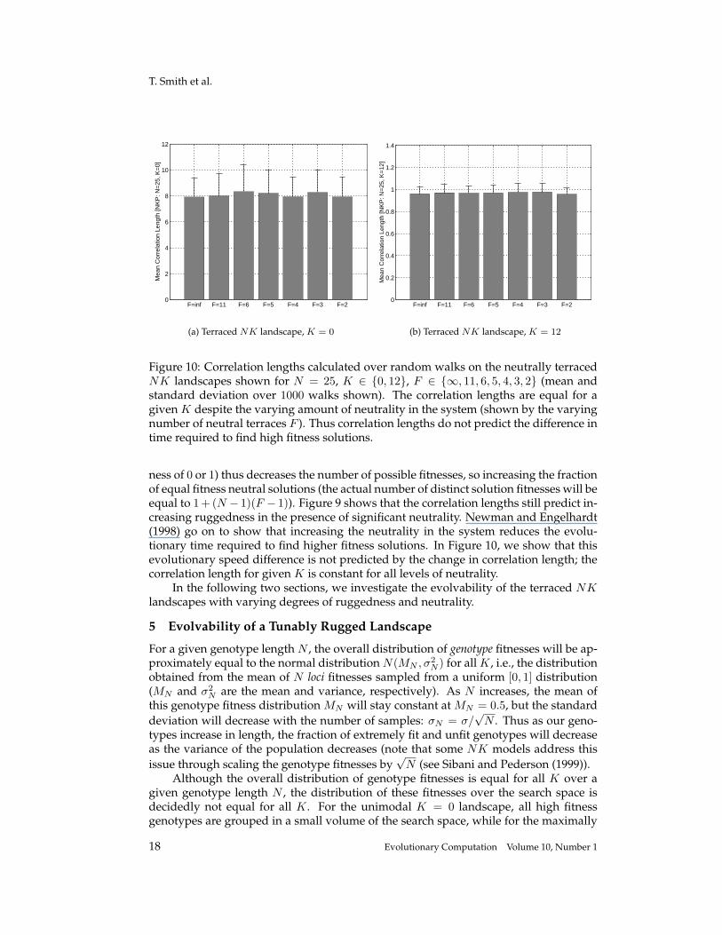
Figure 10: Correlation lengths calculated over random walks on the neutrally terracedNK landscapes shown for N = 25, K ∈ {0, 12}, F ∈ {∞, 11, 6, 5, 4, 3, 2} (mean andstandard deviation over 1000 walks shown). The correlation lengths are equal for agiven K despite the varying amount of neutrality in the system (shown by the varyingnumber of neutral terraces F ). Thus correlation lengths do not predict the difference intime required to find high fitness solutions.
ness of 0 or 1) thus decreases the number of possible fitnesses, so increasing the fractionof equal fitness neutral solutions (the actual number of distinct solution fitnesses will beequal to 1+ (N − 1)(F − 1)). Figure 9 shows that the correlation lengths still predict in-creasing ruggedness in the presence of significant neutrality. Newman and Engelhardt(1998) go on to show that increasing the neutrality in the system reduces the evolu-tionary time required to find higher fitness solutions. In Figure 10, we show that thisevolutionary speed difference is not predicted by the change in correlation length; thecorrelation length for given K is constant for all levels of neutrality.
In the following two sections, we investigate the evolvability of the terraced NKlandscapes with varying degrees of ruggedness and neutrality.
5 Evolvability of a Tunably Rugged Landscape
For a given genotype length N , the overall distribution of genotype fitnesses will be ap-proximately equal to the normal distribution N(MN , σ2
N ) for all K, i.e., the distributionobtained from the mean of N loci fitnesses sampled from a uniform [0, 1] distribution(MN and σ2
N are the mean and variance, respectively). As N increases, the mean ofthis genotype fitness distribution MN will stay constant at MN = 0.5, but the standarddeviation will decrease with the number of samples: σN = σ/
√N . Thus as our geno-
types increase in length, the fraction of extremely fit and unfit genotypes will decreaseas the variance of the population decreases (note that some NK models address thisissue through scaling the genotype fitnesses by
√N (see Sibani and Pederson (1999)).
Although the overall distribution of genotype fitnesses is equal for all K over agiven genotype length N , the distribution of these fitnesses over the search space isdecidedly not equal for all K. For the unimodal K = 0 landscape, all high fitnessgenotypes are grouped in a small volume of the search space, while for the maximally
18 Evolutionary Computation Volume 10, Number 1
Fitness Landscapes and Evolvability
multimodal K = N − 1 landscape, the fitness distribution over the search space israndom. In general, the distribution of fitnesses neighboring a solution of given fit-ness is approximately normal with mean and deviation dependent on N, K and thecurrent solution fitness (see Weinberger (1990) and Stadler and Schnabl (1992)). Fromthis it is possible to derive the expected fitnesses (and the time taken on both adap-tive and random walks) at which local optima are reached for various N and K (again,see Weinberger (1990) and Stadler and Schnabl (1992)). In the next section, we deriveanalytic and empirical results for the evolvability measures when applied to the NKlandscapes.
5.1 Analytically Derived Evolvability for NK Landscapes
In this section, we focus on the probability that an offspring derived from a single bitmutation of the parent has a higher (or equal) fitness than the parent, i.e., the firstevolvability metric Ea (Section 3.1), as a function of the parental fitness. The otherevolvability metrics derived in Section 3 can be similarly treated. Consider a parentgenotype of fitness F0, the mean of the N locus fitnesses fi drawn from a uniformdistribution over [0, 1]:
F0 =1N
N∑
i=1
fi where fi ∈ U [0, 1] (20)
Now, the probability that the offspring fitness F1 is not lower than the parent fit-ness is simply the probability that the K + 1 loci affected by a single bit mutation donot, on average, decrease in fitness:
Ea ≡ P (F1 ≥ F0) = P
((1
K + 1
K+1∑
i=1
fi
)≥ F0
)where fi ∈ U [0, 1] (21)
is the probability that the mean of K + 1 uniformly distributed samples is not smallerthan the current fitness. For the unimodal K = 0 we can solve trivially
P (F1 ≥ F0) = P (f1 ≥ F0) = 1− F0 where f1 ∈ U [0, 1] (22)
For K � 0, the mean of affected loci fitnesses tends to a normal distribution withmean MK+1 = 0.5 and deviation σK+1 = σ/
√K + 1 (where σ is the deviation of loci
fitnesses as K → ∞, assumed to be non-zero and finite). For a normal distributionN(M,σ2), the probability density function n is given by
n =1σ
φ
(x−M
σ
)(23)
where φ(z) =1√2π
exp (−0.5z2) (24)
The probability that a random number drawn from this distribution is greater thansome value F0 is given by the integral of the probability density function over the rele-vant limits (with mean M = 0.5 and deviation σK+1 = σ/
√K + 1):
P (F1 ≥ F0) =√
K + 1σ
∫ ∞
F0
φ
(√K + 1(x− 0.5)
σ
)dx (25)
=
√K + 12πσ2
∫ ∞
F0
exp(−(K + 1)
2σ2(x− 0.5)2
)dx (26)
Evolutionary Computation Volume 10, Number 1 19

T. Smith et al.
0.2 0.3 0.4 0.5 0.6 0.7 0.8 0.90
10
20
30
40
50
60
70
80
90
100
Original Fitness F0
50 e
rfc
( C
( F
0 − 0
.5 )
)C=2 C=4 C=8 C=16
(a) Analytically derived probability of a non-deleterious mutation Ea
0.2 0.3 0.4 0.5 0.6 0.7 0.8 0.90
10
20
30
40
50
60
70
80
90
100
Original Fitness
Pro
b(F
mut
≥ F
curr
ent)
K=0 K=6 K=12K=24
(b) Empirically derived probability of a non-deleterious mutation Ea
Figure 11: Analytically and empirically derived probabilities of a nondeleterious mu-tation Ea. The derived probability is plotted as 50erfc(C(F0 − 0.5)). The empiricalprobability is calculated on the NK landscape with N = 25, K ∈ {0, 6, 12, 24} for arandom sample set of solutions.
which is simply the complementary error function erfc(x):
erfc(x) ≡ 2√π
∫ ∞
x
exp (−z2) dz (27)
and P (F1 ≥ F0) = 0.5 erfc
(√K + 12σ2
(F0 − 0.5)
)(28)
Note that an equivalent result to Equation 28 is derived by Stadler and Schnabl(1992) in order to calculate the probability of solutions of given fitness being local op-tima; Section 3.5.3 describes the link between the fitness evolvability portraits and gen-eral landscape features.
5.2 Empirically Derived Evolvability for NK Landscapes
Figure 11 shows data generated from Equation 28 compared to the fitness evolvabil-ity portraits derived from empirical random sampling of simulated NK landscapes(N = 25, K ∈ {0, 1, 2, 6, 12, 24}), showing good agreement between the analyticallyand empirically derived data. All NK random sample sets used in this paper consistof 1000 individuals sampled from each of 100 generated landscapes – a total of 100, 000sampled solutions. Note that for each set of N,K, there is an arbitrarily large numberof fitness lookup tables that can be generated, and thus an arbitrarily large number ofpossible landscapes. For this reason, we sample both a set of individuals and a set oflandscapes for each value of N, K.
Both sets of data predict that as K increases, the probability of finding a fittermutant increases for parent fitnesses below the population mean of 0.5. Only for parentfitnesses above this mean value of 0.5 does the probability of reaching a fitter mutantfavor the lower K landscapes. This can be understood by considering that a single bitflip mutation can affect the fitness F0 by a fraction of order O(K+1
N ). Low K landscapes
20 Evolutionary Computation Volume 10, Number 1
Fitness Landscapes and Evolvability
0.2 0.3 0.4 0.5 0.6 0.7 0.8 0.90
10
20
30
40
50
60
70
80
90
100
Original Fitness
Pro
b(F
mut
≥ F
curr
ent)
K=0 K=6 K=12K=24
(a) Probability of a nondeleterious mutation Ea
0.2 0.3 0.4 0.5 0.6 0.7 0.8 0.90.3
0.35
0.4
0.45
0.5
0.55
0.6
0.65
0.7
0.75
Original Fitness
< F
0,10
0 >
K=0 K=6 K=12K=24
(b) Expected fitness over all mutations Eb
0.2 0.3 0.4 0.5 0.6 0.7 0.8 0.90.3
0.35
0.4
0.45
0.5
0.55
0.6
0.65
0.7
0.75
Original Fitness
< F
75,1
00 >
K=0 K=6 K=12K=24
(c) Expected fitness over top quartile of muta-tions Ec
0.2 0.3 0.4 0.5 0.6 0.7 0.8 0.90.25
0.3
0.35
0.4
0.45
0.5
0.55
0.6
0.65
0.7
Original Fitness
< F
0,25
>
K=0 K=6 K=12K=24
(d) Expected fitness over bottom quartile of mu-tations Ed
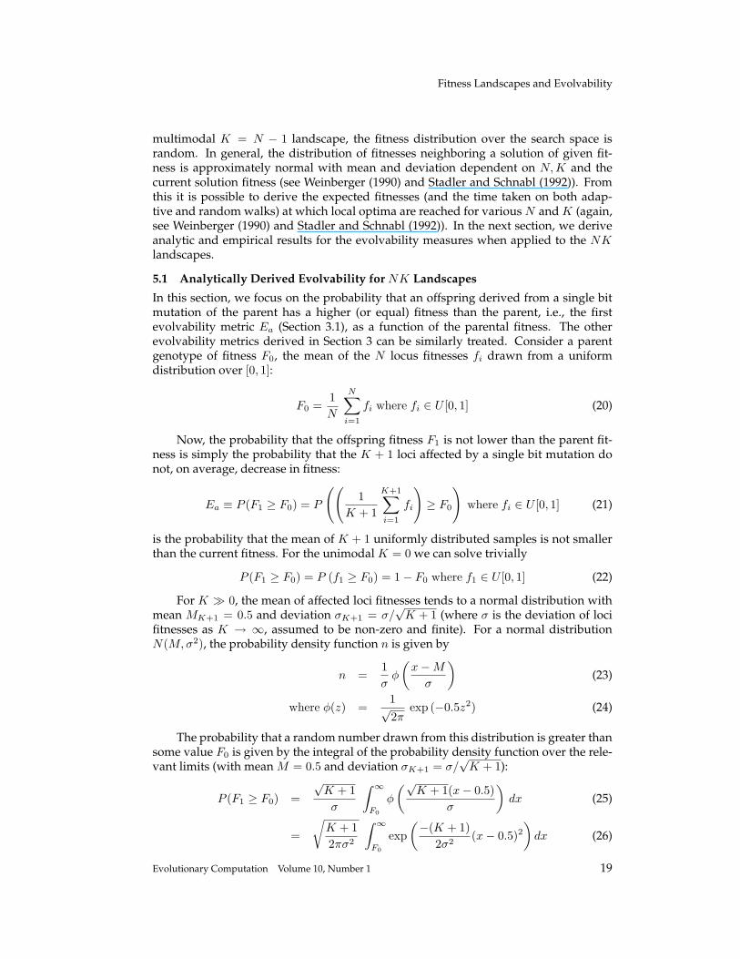
Figure 12: Fitness evolvability portraits for the NK landscapes with N = 25, K ∈{0, 6, 12, 24}. The evolvability metrics were calculated from a random sample set ofsolutions.
are thus highly correlated3, and offspring fitnesses are close to parent fitnesses. For highK landscapes, the offspring-parent fitnesses are less correlated, thus offspring fitnesseson average are close to the population mean of 0.5, and the distribution of genotypefitnesses is essentially random in space.
The other evolvability measures can be derived in similar fashion and give goodagreement with the fitness evolvability portraits derived from empirical simulationof the NK landscapes. Figure 12 shows empirical data for the evolvability metricsEa, Eb, Ec, Ed. First, we correctly identify the increasing modality of the spaces at higherfitnesses with increasing K; as fitness increases, the probability of nondeleterious mu-tations Ea tails off faster for high K than for low K, showing that the number of localoptima increase extremely rapidly above fitnesses of 0.5 for K = N − 1. Second, the
3The offspring-parent correlation is simply ρ = 1 − K+1N
(Weinberger, 1990) with the correlation lengthτ = −1/ ln(ρ).
Evolutionary Computation Volume 10, Number 1 21
T. Smith et al.
0.2 0.3 0.4 0.5 0.6 0.7 0.8 0.90
10
20
30
40
50
60
70
80
90
100
Original Fitness
Pro
b(F
mut
≥ F
curr
ent)
K=0 K=6 K=12K=24
(a) Probability of a nondeleterious mutation Ea
0.2 0.3 0.4 0.5 0.6 0.7 0.8 0.90.2
0.3
0.4
0.5
0.6
0.7
0.8
0.9
Original Fitness
< F
0,10
0 >
K=0 K=6 K=12K=24
(b) Expected fitness over all mutations Eb
0.2 0.3 0.4 0.5 0.6 0.7 0.8 0.90.3
0.35
0.4
0.45
0.5
0.55
0.6
0.65
0.7
0.75
0.8
Original Fitness
< F
75,1
00 >
K=0 K=6 K=12K=24
(c) Expected fitness over top quartile of muta-tions Ec
0.2 0.3 0.4 0.5 0.6 0.7 0.8 0.90.2
0.3
0.4
0.5
0.6
0.7
0.8
0.9
Original Fitness
< F
0,25
>K=0 K=6 K=12K=24
(d) Expected fitness over bottom quartile of mu-tations Ed
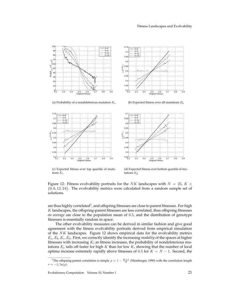
Figure 13: Fitness evolvability portraits for the terraced NK landscapes with N = 25,K ∈ {0, 6, 12, 24}, F = 4. The evolvability metrics were calculated from a randomsample set of solutions.
portraits correctly predict the increasing ruggedness of the spaces with increasing K; theexpected offspring fitness graphs (Eb shown in Figure 12(c)) show decreasing gradientwith increased K (remember from Section 3.5.3 that this gradient is proportional to theautocorrelation function).
The next section applies the evolvability analysis to the tunably neutral terracedNK landscapes.
6 Evolvability of a Tunably Neutral Landscape
In the previous section, we saw how we can discriminate between landscapes of vary-ing ruggedness using the fitness evolvability portraits derived in Section 3.1. In thissection, we derive portraits for the tunably neutral terraced NK landscape (Section 4)in order to discriminate between landscapes of varying ruggedness in the presence of
22 Evolutionary Computation Volume 10, Number 1
Fitness Landscapes and Evolvability
0.1 0.2 0.3 0.4 0.5 0.6 0.7 0.8 0.910
20
30
40
50
60
70
80
90
100
Original Fitness
Pro
b(F
mut
≥ F
curr
ent)
F=2 F=3 F=6 F=∞
(a) Probability of a nondeleterious mutation Ea
for K = 0
0.1 0.2 0.3 0.4 0.5 0.6 0.7 0.8 0.90.1
0.2
0.3
0.4
0.5
0.6
0.7
0.8
0.9
Original Fitness
< F
0,10
0 >
F=2 F=3 F=6 F=∞
(b) Expected fitness over all mutations Eb forK = 0
0.1 0.2 0.3 0.4 0.5 0.6 0.7 0.8 0.90
10
20
30
40
50
60
70
80
90
100
Original Fitness
Pro
b(F
mut
≥ F
curr
ent)
F=2 F=3 F=6 F=∞
(c) Probability of a nondeleterious mutation Ea
for K = 12
0.1 0.2 0.3 0.4 0.5 0.6 0.7 0.8 0.90.3
0.35
0.4
0.45
0.5
0.55
0.6
0.65
0.7
Original Fitness
< F
0,10
0 >F=2 F=3 F=6 F=∞
(d) Expected fitness over all mutations Eb forK = 12
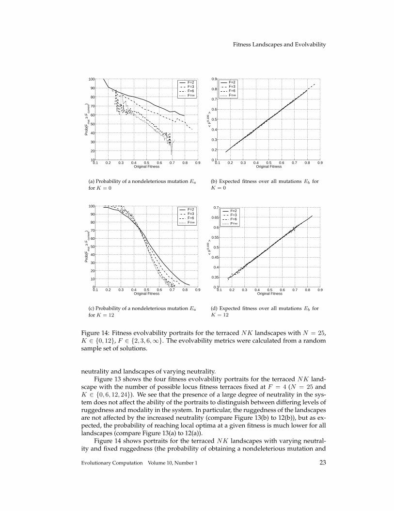
Figure 14: Fitness evolvability portraits for the terraced NK landscapes with N = 25,K ∈ {0, 12}, F ∈ {2, 3, 6,∞}. The evolvability metrics were calculated from a randomsample set of solutions.
neutrality and landscapes of varying neutrality.Figure 13 shows the four fitness evolvability portraits for the terraced NK land-
scape with the number of possible locus fitness terraces fixed at F = 4 (N = 25 andK ∈ {0, 6, 12, 24}). We see that the presence of a large degree of neutrality in the sys-tem does not affect the ability of the portraits to distinguish between differing levels ofruggedness and modality in the system. In particular, the ruggedness of the landscapesare not affected by the increased neutrality (compare Figure 13(b) to 12(b)), but as ex-pected, the probability of reaching local optima at a given fitness is much lower for alllandscapes (compare Figure 13(a) to 12(a)).
Figure 14 shows portraits for the terraced NK landscapes with varying neutral-ity and fixed ruggedness (the probability of obtaining a nondeleterious mutation and
Evolutionary Computation Volume 10, Number 1 23
T. Smith et al.
the expected fitness of all mutations for N = 25, K ∈ {0, 12}, F ∈ {2, 3, 6,∞}). Wesee that the expected mutation fitness (Figures 14(b) and 14(d)) does not change withdiffering levels of neutrality in the system; tallying with the results that the autocorre-lation and ruggedness do not change with neutrality in the NK landscapes. However,the probability of obtaining a nondeleterious mutation (Figures 14(a) and 14(c)) doesshow such change. As F → 2, neutrality increases and the probability of obtaininga nondeleterious mutation increases. For K = 0, even at high fitnesses there are stillon average 1/F neutral mutations. For high K, this probability tends to zero at highfitnesses as all K + 1 loci fitness affected by the mutation need to show a neutral mu-tation. However, this decrease in the probability of finding nondeleterious mutationsis slower for landscapes with more neutrality. The difference is significant: at a fitnessof 0.6, roughly 37% of mutations in the F = 2 landscape are nondeleterious comparedwith roughly 13% of such mutations for the non-neutral F = ∞ landscape. At a fitnessof 0.7, the corresponding percentages are roughly 18% and 0%. Thus, in the highly neu-tral F = 2 landscape, the probability of the search process reaching a local optimumis significantly smaller than the probability of reaching a local optimum in the non-neutral F = ∞. Rather than sticking in local optima, the search process can exploremore of the space along neutral networks, eventually reaching higher fitness solutions.
Thus the fitness evolvability portraits do indeed differentiate between landscapesof both varying ruggedness (with constant neutrality) and varying neutrality (with con-stant ruggedness). In particular, two general features are seen for the terraced NKlandscapes with the portrait descriptions. First, as neutrality increases, the landscaperuggedness does not change, as evidenced by the expected offspring fitness portrait(this result is also shown with the correlation lengths shown in Figure 10). Second, asneutrality increases, the number of nondeleterious mutations increases at all levels offitness and for all K. Thus as expected, the number of local optima falls with increasingneutrality, but also the number of local optima decrease at all fitness levels in the space.
In the next section, we show that fitness evolvability portraits based on samplescollected during simple hill-climbing optimization show the same features as whenbased on the random samples used in the previous two sections. This is crucial forproblems with extremely skewed solution fitness distributions for which random sam-pling is inappropriate and biased sampling techniques must be used. If we are to de-scribe the landscape structure of such problems, the portraits must be robust whenbased on such biased samples.
7 Online Sampling Evolvability
In the previous sections, we have investigated empirically derived evolvabilities forthe tunably rugged and tunably neutral terraced NK landscapes through random sam-pling of the space of all solutions. This random sampling technique works well withthe NK landscapes where solution fitnesses are defined as the linear sum of all locifitnesses; due to the central limit theorem, the solution fitnesses will be approximatelynormally distributed. However, in many problems, such normally distributed solu-tion fitnesses will not be encountered, and measures based on random sampling of thespace may in general be less successful in describing the landscape.
With such skewed solution fitness distributions, it may be necessary to bias the col-lected sample through keeping only a percentage of solutions found at each fitness anddefine the landscape description over this biased sample. With even more extremelyskewed distributions, it may be necessary to collect a biased sample through some di-rect search optimization procedure such as a simple hill-climber. For example, Smith
24 Evolutionary Computation Volume 10, Number 1
Fitness Landscapes and Evolvability
0.3 0.4 0.5 0.6 0.7 0.80
10
20
30
40
50
60
70
80
90
100
Original Fitness
Pro
b(F
mut
≥ F
curr
ent)
K=0 K=6 K=12K=24
(a) Probability of a nondeleterious mutation Ea
0.3 0.4 0.5 0.6 0.7 0.80.35
0.4
0.45
0.5
0.55
0.6
0.65
0.7
0.75
Original Fitness
< F
0,10
0 >
K=0 K=6 K=12K=24
(b) Expected fitness over all mutations Eb
Figure 15: Fitness evolvability portraits for the NK landscapes with N = 25, K ∈{0, 6, 12, 24}. The evolvability metrics were calculated from a sample set of solutionscollected during hill-climbing.
et al. (2001a) find only 0.0001% of randomly generated solutions have fitness above 50%of the maximum in a neural network robot control problem despite this fitness beingrelatively easy to reach using optimization techniques.
In this section, we show that the fitness evolvability portraits presented in the pre-vious sections still describe the general features of the terraced NK landscapes whenbased on a biased sample collected using a (1+1) evolutionary strategy hill-climber(Rechenberg, 1973). 100 runs of the hill-climber were performed for each parametersetting (generating a new landscape for each run). From an initial randomly generatedsolution, random mutations were applied (using both single bit mutation and mutationprobability per bit gives similar results) with nondeleterious mutations accepted anddeleterious mutations rejected. All new encountered genotypes were saved for analy-sis, and the hill-climber stopped after 1, 000 mutations had been tried. The followinganalysis uses the saved samples over each parameter setting.
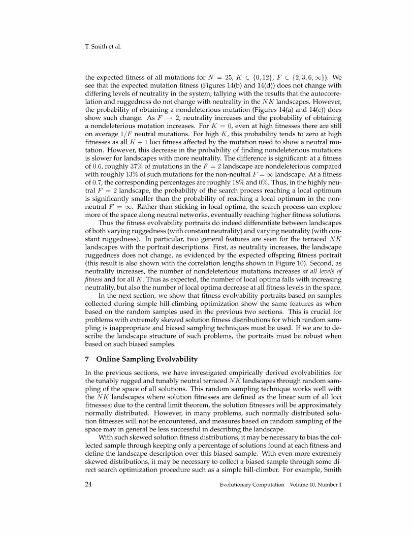
Figure 15 shows the probability of a nondeleterious mutation and the expectedmutation fitness over the NK landscape with N = 25, K ∈ {0, 6, 12, 24} for the biasedhill-climber sample. As seen with the fitness evolvability portraits based on randomsampling, the ruggedness of the landscape, as measured through the gradient of theexpected mutation fitness against fitnesses, increases with K. Also, the number of localoptima increases with both K and the level of fitness.
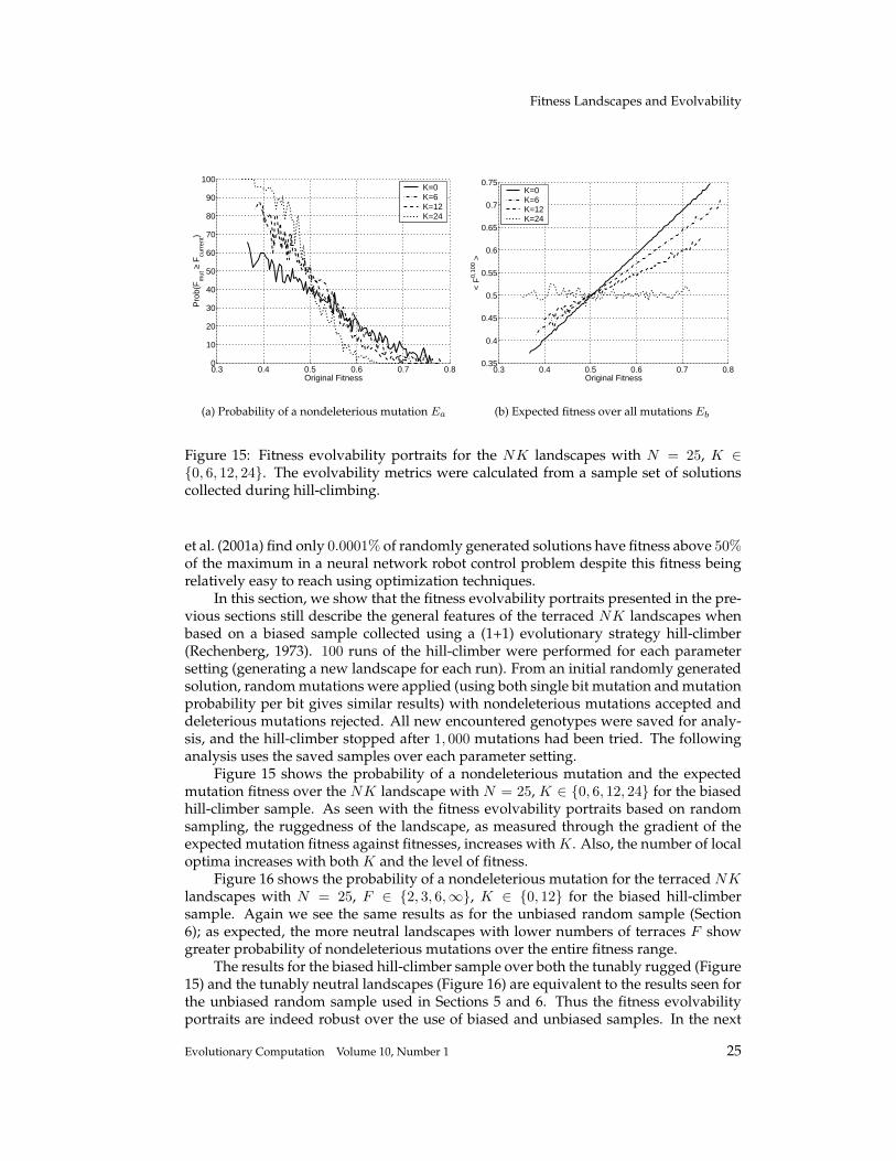
Figure 16 shows the probability of a nondeleterious mutation for the terraced NKlandscapes with N = 25, F ∈ {2, 3, 6,∞}, K ∈ {0, 12} for the biased hill-climbersample. Again we see the same results as for the unbiased random sample (Section6); as expected, the more neutral landscapes with lower numbers of terraces F showgreater probability of nondeleterious mutations over the entire fitness range.
The results for the biased hill-climber sample over both the tunably rugged (Figure15) and the tunably neutral landscapes (Figure 16) are equivalent to the results seen forthe unbiased random sample used in Sections 5 and 6. Thus the fitness evolvabilityportraits are indeed robust over the use of biased and unbiased samples. In the next
Evolutionary Computation Volume 10, Number 1 25
T. Smith et al.
0.2 0.3 0.4 0.5 0.6 0.7 0.8 0.9 10
10
20
30
40
50
60
70
80
90
100
Original Fitness
Pro
b(F
mut
≥ F
curr
ent)
F=2 F=3 F=6 F=∞
(a) Probability of a nondeleterious mutation Ea
for K = 0
0.2 0.3 0.4 0.5 0.6 0.7 0.8 0.9 10
10
20
30
40
50
60
70
80
90
100
Original Fitness
Pro
b(F
mut
≥ F
curr
ent)
F=2 F=3 F=6 F=∞
(b) Probability of a nondeleterious mutation Ea
for K = 12
Figure 16: Fitness evolvability portraits for the terraced NK landscapes with N = 25,K ∈ {0, 12}, F ∈ {2, 3, 6,∞}. The evolvability metrics were calculated from a sampleset of solutions collected during hill-climbing.
section, we derive the fitness evolvability portraits for a real search space from theevolutionary hardware domain, evolution of a digital inverter circuit, and comparewith results from optimization runs.
8 An Evolutionary Hardware Problem
In this section, we apply the same evolvability analysis to search spaces correspond-ing to real engineering applications and compare with results from optimization runs.It should be emphasized that the specific implementation details outlined below areunimportant; what should be stressed is that the two different search spaces correspondto two solution representations, “multiplex” and “direct”, for the same evolutionaryelectronics problem.
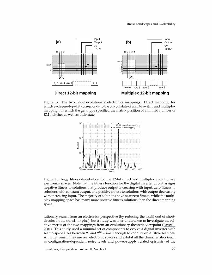
In Layzell (1999, 2001), various electronic circuits were evolved directly in hard-ware using an Evolvable Motherboard (EM); a purpose-built research platform con-sisting of bipolar transistors connected to a triangular matrix of reconfigurable analogswitches. The triangular switch matrix allows all possible combinations of intercon-nection between the transistors, power supply, and I/O, but by altering the genotype-to-phenotype mapping, various more restrictive interconnection architectures can beinvestigated. This research explored two different architectures: direct mapping, forwhich each genotype bit corresponds to the on/off state of an EM switch, and multi-plex mapping, for which the genotype specified the matrix position of a limited numberof EM switches as well as their state. Figure 17 shows how the two mappings differ inthe way that the state of the EM switches are specified.
Circuit evolution was carried out both in the noisy environment of physical hard-ware and a noise-free environment attained by simulating the EM with proprietaryelectronics design software. In general, this research required search-spaces of the or-der 21000 in size, with the multiplex mapping consistently proving more conducive toevolutionary search. Multiplex mapping was originally designed to improve the evo-
26 Evolutionary Computation Volume 10, Number 1
Fitness Landscapes and Evolvability
row 0123
�
c� ol 0 1 2
r0,c0 r3,c2r0,c2r0,c1
c� ol 0 1 2 3�
(a) (b)
row 0 row 1 row 2 row 5
row 0123
�
5�4
Direct 12-bit mapping Multiplex 12-bit mapping
Input Output 0V +2.8V
Input Output 0V +2.8V
Figure 17: The two 12-bit evolutionary electronics mappings. Direct mapping, forwhich each genotype bit corresponds to the on/off state of an EM switch, and multiplexmapping, for which the genotype specified the matrix position of a limited number ofEM switches as well as their state.
−5000 −4000 −3000 −2000 −1000 0 1000 2000 300010
−3
10−2
10−1
100
fitness
frac
tion
12−bit multiplex mapping12−bit direct mapping
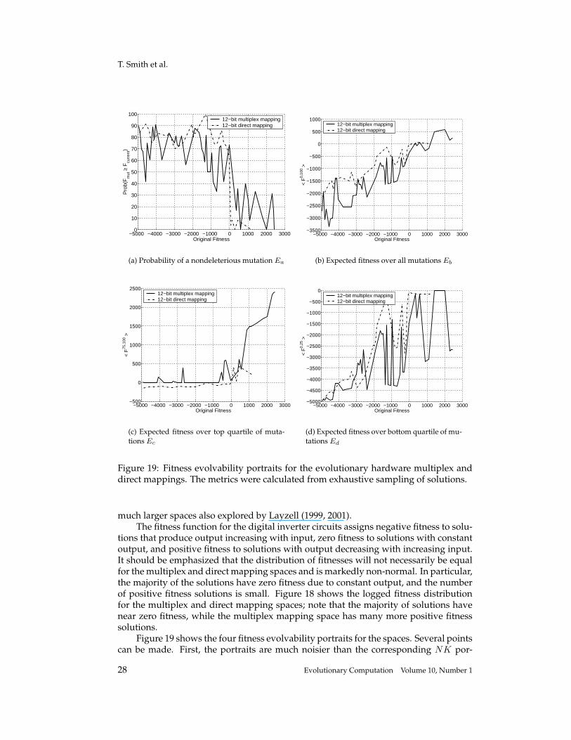
Figure 18: log10 fitness distribution for the 12-bit direct and multiplex evolutionaryelectronics spaces. Note that the fitness function for the digital inverter circuit assignsnegative fitness to solutions that produce output increasing with input, zero fitness tosolutions with constant output, and positive fitness to solutions with output decreasingwith increasing input. The majority of solutions have near zero fitness, while the multi-plex mapping space has many more positive fitness solutions than the direct mappingspace.
lutionary search from an electronics perspective (by reducing the likelihood of short-circuits on the transistor pins), but a study was later undertaken to investigate the rel-ative merits of the two mappings from an evolutionary theoretic viewpoint (Layzell,2001). This study used a minimal set of components to evolve a digital inverter withsearch-space sizes between 28 and 216 – small enough to conduct exhaustive searches.Although small, they are real electronic spaces and exhibit all the characteristics (suchas configuration-dependent noise levels and power-supply related epistasis) of the
Evolutionary Computation Volume 10, Number 1 27
T. Smith et al.
−5000 −4000 −3000 −2000 −1000 0 1000 2000 30000
10
20
30
40
50
60
70
80
90
100
Original Fitness
Pro
b(F
mut
≥ F
curr
ent)
12−bit multiplex mapping12−bit direct mapping
(a) Probability of a nondeleterious mutation Ea
−5000 −4000 −3000 −2000 −1000 0 1000 2000 3000−3500
−3000
−2500
−2000
−1500
−1000
−500
0
500
1000
Original Fitness
< F
0,10
0 >
12−bit multiplex mapping12−bit direct mapping
(b) Expected fitness over all mutations Eb
−5000 −4000 −3000 −2000 −1000 0 1000 2000 3000−500
0
500
1000
1500
2000
2500
Original Fitness
< F
75,1
00 >
12−bit multiplex mapping12−bit direct mapping
(c) Expected fitness over top quartile of muta-tions Ec
−5000 −4000 −3000 −2000 −1000 0 1000 2000 3000−5000
−4500
−4000
−3500
−3000
−2500
−2000
−1500
−1000
−500
0
Original Fitness
< F
0,25
>
12−bit multiplex mapping12−bit direct mapping
(d) Expected fitness over bottom quartile of mu-tations Ed
Figure 19: Fitness evolvability portraits for the evolutionary hardware multiplex anddirect mappings. The metrics were calculated from exhaustive sampling of solutions.
much larger spaces also explored by Layzell (1999, 2001).The fitness function for the digital inverter circuits assigns negative fitness to solu-
tions that produce output increasing with input, zero fitness to solutions with constantoutput, and positive fitness to solutions with output decreasing with increasing input.It should be emphasized that the distribution of fitnesses will not necessarily be equalfor the multiplex and direct mapping spaces and is markedly non-normal. In particular,the majority of the solutions have zero fitness due to constant output, and the numberof positive fitness solutions is small. Figure 18 shows the logged fitness distributionfor the multiplex and direct mapping spaces; note that the majority of solutions havenear zero fitness, while the multiplex mapping space has many more positive fitnesssolutions.
Figure 19 shows the four fitness evolvability portraits for the spaces. Several pointscan be made. First, the portraits are much noisier than the corresponding NK por-
28 Evolutionary Computation Volume 10, Number 1
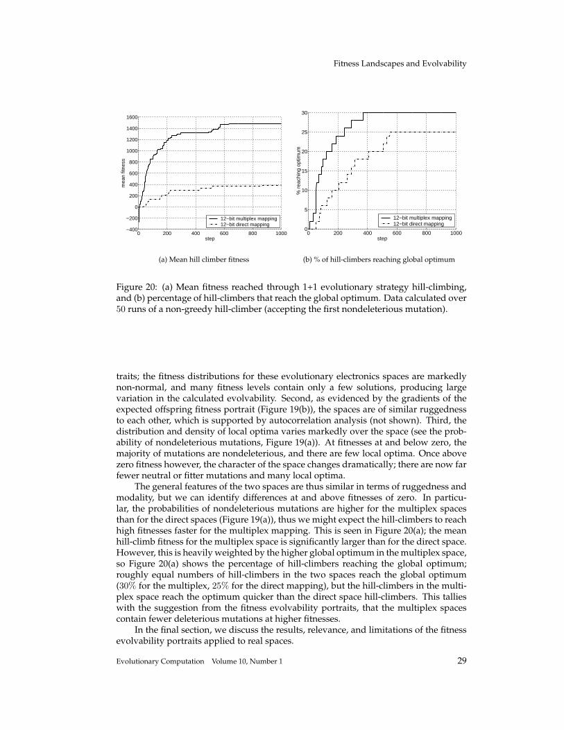
Fitness Landscapes and Evolvability
0 200 400 600 800 1000−400
−200
0
200
400
600
800
1000
1200
1400
1600
step
mea
n fit
ness
12−bit multiplex mapping12−bit direct mapping
(a) Mean hill climber fitness
0 200 400 600 800 10000
5
10
15
20
25
30
step
% r
each
ing
optim
um
12−bit multiplex mapping12−bit direct mapping
(b) % of hill-climbers reaching global optimum
Figure 20: (a) Mean fitness reached through 1+1 evolutionary strategy hill-climbing,and (b) percentage of hill-climbers that reach the global optimum. Data calculated over50 runs of a non-greedy hill-climber (accepting the first nondeleterious mutation).
traits; the fitness distributions for these evolutionary electronics spaces are markedlynon-normal, and many fitness levels contain only a few solutions, producing largevariation in the calculated evolvability. Second, as evidenced by the gradients of theexpected offspring fitness portrait (Figure 19(b)), the spaces are of similar ruggednessto each other, which is supported by autocorrelation analysis (not shown). Third, thedistribution and density of local optima varies markedly over the space (see the prob-ability of nondeleterious mutations, Figure 19(a)). At fitnesses at and below zero, themajority of mutations are nondeleterious, and there are few local optima. Once abovezero fitness however, the character of the space changes dramatically; there are now farfewer neutral or fitter mutations and many local optima.
The general features of the two spaces are thus similar in terms of ruggedness andmodality, but we can identify differences at and above fitnesses of zero. In particu-lar, the probabilities of nondeleterious mutations are higher for the multiplex spacesthan for the direct spaces (Figure 19(a)), thus we might expect the hill-climbers to reachhigh fitnesses faster for the multiplex mapping. This is seen in Figure 20(a); the meanhill-climb fitness for the multiplex space is significantly larger than for the direct space.However, this is heavily weighted by the higher global optimum in the multiplex space,so Figure 20(a) shows the percentage of hill-climbers reaching the global optimum;roughly equal numbers of hill-climbers in the two spaces reach the global optimum(30% for the multiplex, 25% for the direct mapping), but the hill-climbers in the multi-plex space reach the optimum quicker than the direct space hill-climbers. This tallieswith the suggestion from the fitness evolvability portraits, that the multiplex spacescontain fewer deleterious mutations at higher fitnesses.
In the final section, we discuss the results, relevance, and limitations of the fitnessevolvability portraits applied to real spaces.
Evolutionary Computation Volume 10, Number 1 29
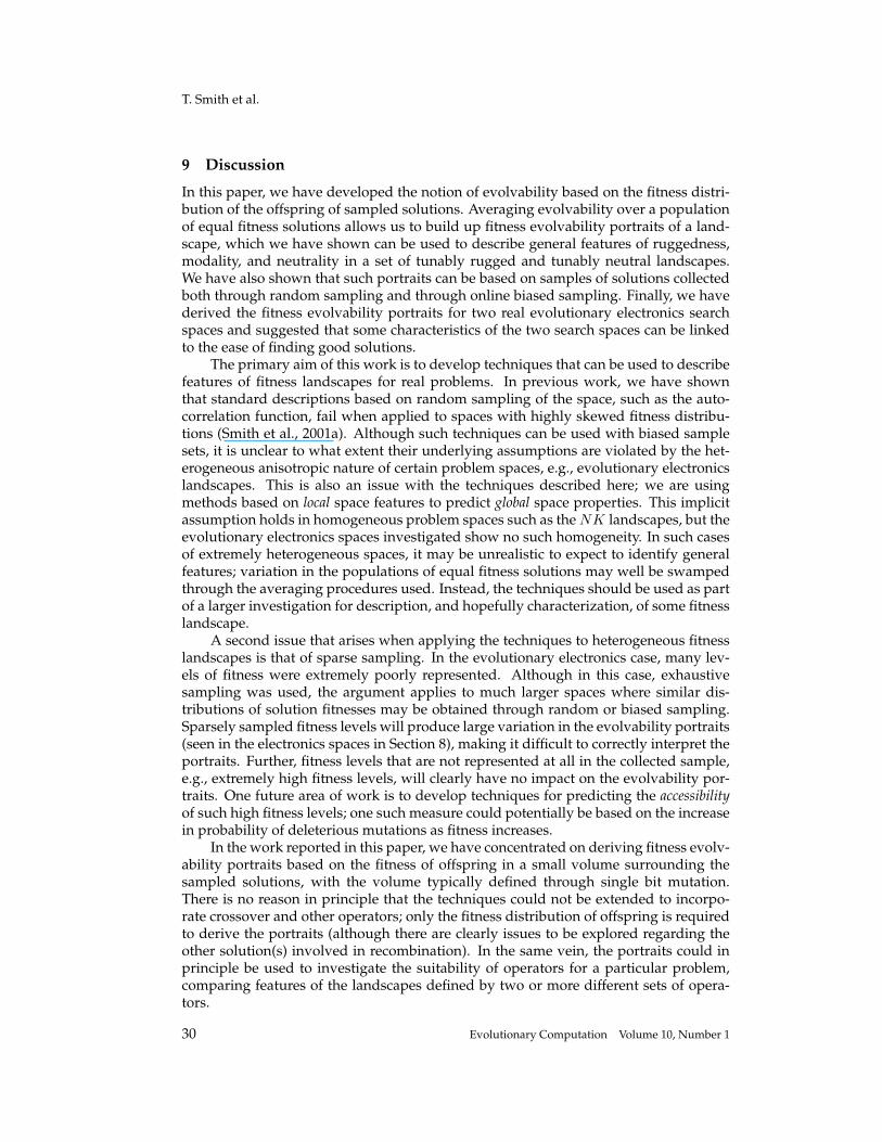
T. Smith et al.
9 Discussion
In this paper, we have developed the notion of evolvability based on the fitness distri-bution of the offspring of sampled solutions. Averaging evolvability over a populationof equal fitness solutions allows us to build up fitness evolvability portraits of a land-scape, which we have shown can be used to describe general features of ruggedness,modality, and neutrality in a set of tunably rugged and tunably neutral landscapes.We have also shown that such portraits can be based on samples of solutions collectedboth through random sampling and through online biased sampling. Finally, we havederived the fitness evolvability portraits for two real evolutionary electronics searchspaces and suggested that some characteristics of the two search spaces can be linkedto the ease of finding good solutions.
The primary aim of this work is to develop techniques that can be used to describefeatures of fitness landscapes for real problems. In previous work, we have shownthat standard descriptions based on random sampling of the space, such as the auto-correlation function, fail when applied to spaces with highly skewed fitness distribu-tions (Smith et al., 2001a). Although such techniques can be used with biased samplesets, it is unclear to what extent their underlying assumptions are violated by the het-erogeneous anisotropic nature of certain problem spaces, e.g., evolutionary electronicslandscapes. This is also an issue with the techniques described here; we are usingmethods based on local space features to predict global space properties. This implicitassumption holds in homogeneous problem spaces such as the NK landscapes, but theevolutionary electronics spaces investigated show no such homogeneity. In such casesof extremely heterogeneous spaces, it may be unrealistic to expect to identify generalfeatures; variation in the populations of equal fitness solutions may well be swampedthrough the averaging procedures used. Instead, the techniques should be used as partof a larger investigation for description, and hopefully characterization, of some fitnesslandscape.
A second issue that arises when applying the techniques to heterogeneous fitnesslandscapes is that of sparse sampling. In the evolutionary electronics case, many lev-els of fitness were extremely poorly represented. Although in this case, exhaustivesampling was used, the argument applies to much larger spaces where similar dis-tributions of solution fitnesses may be obtained through random or biased sampling.Sparsely sampled fitness levels will produce large variation in the evolvability portraits(seen in the electronics spaces in Section 8), making it difficult to correctly interpret theportraits. Further, fitness levels that are not represented at all in the collected sample,e.g., extremely high fitness levels, will clearly have no impact on the evolvability por-traits. One future area of work is to develop techniques for predicting the accessibilityof such high fitness levels; one such measure could potentially be based on the increasein probability of deleterious mutations as fitness increases.
In the work reported in this paper, we have concentrated on deriving fitness evolv-ability portraits based on the fitness of offspring in a small volume surrounding thesampled solutions, with the volume typically defined through single bit mutation.There is no reason in principle that the techniques could not be extended to incorpo-rate crossover and other operators; only the fitness distribution of offspring is requiredto derive the portraits (although there are clearly issues to be explored regarding theother solution(s) involved in recombination). In the same vein, the portraits could inprinciple be used to investigate the suitability of operators for a particular problem,comparing features of the landscapes defined by two or more different sets of opera-tors.
30 Evolutionary Computation Volume 10, Number 1
Fitness Landscapes and Evolvability
Finally, it should be emphasized that the techniques of evolvability and fitnessportraits developed in this paper should be seen as complementary to other methodsfor describing and characterizing fitness landscapes. No single measure or descriptioncan possibly characterize any high-dimensional heterogeneous search space; the fitnessevolvability portraits are presented as a useful method to investigate the properties ofthe fitness landscape over the entire fitness range.
Acknowledgments
The authors would like to thank the three anonymous reviewers. We also thankAndy Philippides, Lionel Barnett, Inman Harvey, and the members of the Centrefor Computational Neuroscience and Robotics (http://www.cogs.sussex.ac.uk/ccnr/)for constructive comments and discussion. We would also like to thank the Sus-sex High Performance Computing Initiative (http://www.hpc.sussex.ac.uk/) for com-puting support. TS is funded by a British Telecom Future Technologies Group(http://innovate.bt.com/projects/ftg.htm) sponsored Biotechnology and Biology Sci-ence Research Council Case Award.
ReferencesAltenberg, L. (1994). The evolution of evolvability in genetic programming. In Kinnear Jr., K.,
editor, Advances in Genetic Programming, Chapter 3, pages 47–74, MIT Press, Cambridge,Massachusetts.
Barnett, L. (1997). Tangled webs–evolutionary dynamics on fitness landscapes with neutrality. Master’sthesis, School of Cognitive and Computing Sciences, University of Sussex,Sussex, UK.
Barnett, L. (1998). Ruggedness and neutrality: The NKp family of fitness landscapes. In Adami,C. et al., editors, Artificial Life VI: Proceedings of the Sixth International Conference on ArtificialLife, pages 18–27, MIT Press, Cambridge, Massachusetts.
Barnett, L. (2001). Statistical properties of the NKp family of fitness landscapes. In press.
Binder, K. and Young, A. (1986). Spin Glasses: Experimental Facts, Theoretical Concepts andOpen Questions. Reviews of Modern Physics, 58(4):801–976.
Burch, C. and Chao, L. (2000). Evolvability of an RNA Virus is Determined by its MutationalNeighbourhood. Nature, 406:625–628.
Cavalli-Sforza, L. and Feldman, M. (1976). Evolution of continuous variation: Direct approachthrough joint distribution of genotypes and phenotypes. Proceedings of the National Academyof Sciences, 73:1689–1692.
Coyne, J., Barton, N., and Turelli, M. (1997). Perspective: A critique of Sewall Wright’s shiftingbalance theory of evolution. Evolution, 51(3):643–671.
Davidor, Y. (1991). Epistasis variance: A viewpoint on GA-hardness. In Rawlins, G., editor, Foun-dations of Genetic Algorithms (FOGA’1), pages 22–35, Morgan Kaufmann, San Mateo, Califor-nia.
Dawkins, R. (1989). The evolution of evolvability. In Langton, C., editor, Artificial Life: Proceedingsof the Interdisciplinary Workshop on the Synthesis and Simulation of Living Systems, Volume VIof Santa Fe Institute Studies in the Sciences of Complexity, pages 201–220, Addison-Wesley,Redwood, California.
Derrida, B. (1981). Random energy model–an exactly solvable model of disordered-systems.Physical Review B, 24(5):2613–2626.
Ebner, M. et al. (2001). On Neutral Networks and Evolvability. In Proceedings of the 2001 Conferenceon Evolutionary Computation: CEC2001, pages 1–8, IEEE Press, Piscataway, New Jersey.
Evolutionary Computation Volume 10, Number 1 31

T. Smith et al.
Eldredge, N. and Gould, S. (1972). Punctuated equilibria: An alternative to phyletic gradualism.In Schopf, T., editor, Models in Paleobiology, pages 82–115, Freeman, San Francisco, California.
Elena, S., Cooper, V., and Lenski, R. (1996). Punctuated evolution caused by selection of rarebeneficial mutations. Science, 272:1802–1804.
Fogel, L., Owens, A., and Walsh, M. (1966). Artificial Intelligence through Simulated Evolution. JohnWiley and Sons, New York, New York.
Forst, C., Reidys, C., and Weber, J. (1995). Neutral networks as model-landscapes for RNAsecondary-structure folding landscapes. In Moran, F. et al., editors, Advances in ArtificialLife: Proceedings of the Third European Conference on Artificial Life, ECAL95, pages 128–147,Springer, Berlin, Germany.
Gould, S. and Eldredge, N. (1977). Punctuated equilibria: The tempo and mode of evolutionreconsidered. Paleobiology, 3:115–151.
Gruner, W. et al. (1996). Analysis of RNA sequence structure maps by exhaustive enumeration:I Neutral networks, II Structures of neutral networks and shape space covering. MonathefteChem., 127:355–374, 375–389.
Harvey, I. and Thompson, A. (1996). Through the labyrinth evolution finds a way: A silicon ridge.In Higuchi, T., editor, Proceedings of the First International Conference on Evolvable Systems:From Biology to Hardware (ICES’96), pages 406–422, Springer, Berlin, Germany.
Holland, J. (1992). Adaptation in Natural and Artificial Systems. Second edition. MIT Press, Cam-bridge, Massachusetts.
Hordijk, W. (1996). A measure of landscapes. Evolutionary Computation, 4(4):335–360.
Huynen, M. (1996). Exploring phenotype space through neutral evolution. Journal of MolecularEvolution, 43:165–169.
Huynen, M., Stadler, P., and Fontana, W. (1996). Smoothness within ruggedness: The role ofneutrality in adaptation. Proceedings of the National Academy of Sciences, 93:394–401.
Jones, T. and Forrest, S. (1995). Fitness distance correlation as a measure of problem difficulty forgenetic algorithms. In Eshelmann, L., editor, Proceedings of the Sixth International Conferenceon Genetic Algorithms (ICGA95), pages 184–192, Morgan Kaufmann, San Mateo, California.
Kauffman, S. (1993). The Origins of Order: Self-Organization and Selection in Evolution. Oxford Uni-versity Press, Oxford, UK.
Kimura, M. (1983). The Neutral Theory of Molecular Evolution. Cambridge University Press, Cam-bridge, UK.
Kirschner, M. and Gerhart, J. (1998). Evolvability. Proceedings of the National Academy of Sciences,95:8420–8427.
Koza, J. (1992). Genetic Programming: On the Programming of Computers by Means of Natural Selec-tion. MIT Press, Cambridge, Massachusetts.
Lawler, E. et al. (1985). The Travelling Salesman Problem. John Wiley and Sons, New York, NewYork.
Layzell, P. (1999). Reducing hardware evolution’s dependency on FPGAs. In Proceedings of theSeventh International Conference on Microelectronics for Neural, Fuzzy and Bio-Inspired Systems,pages 171–178, IEEE Press, Piscataway, New Jersey.
Layzell, P. (2001). Hardware Evolution: On the Nature of Electronic Circuits Derived Through ArtificialEvolution. Ph.D. thesis, School of Cognitive and Computing Sciences, University of Sussex,Sussex, UK.
32 Evolutionary Computation Volume 10, Number 1
Fitness Landscapes and Evolvability
Lipsitch, M. (1991). Adaptation on rugged landscapes generated by iterated local neighboringgenes. In Belew, R. and Booker, L., editors, Proceedings of the Fourth International Conferenceon Genetic Algorithms (ICGA91), pages 128–135, Morgan Kaufmann, San Mateo, California.
Manderick, B., Weger, M., and Spiessens, P. (1991). The genetic algorithm and the structure of thefitness landscape. In Belew, R. and Booker, L., editors, Proceedings of the Fourth InternationalConference on Genetic Algorithms (ICGA91), pages 143–150, Morgan Kaufmann, San Mateo,California.
Marr, D. (1976). Artificial intelligence–a personal view. Technical Report AIM 355, MIT AI Lab,MIT, Cambridge, Massachusetts.
Marrow, P. (1999). Evolvability: Evolution, computation, biology. In Wu, A., editor, Proceedingsof the 1999 Genetic and Evolutionary Computation Conference Workshop Program (GECCO-99Workshop on Evolvability), pages 30–33, Morgan Kaufmann, San Mateo, California.
Naudts, B. and Kallel, L. (2000). A comparison of predictive measures of problem difficulty inevolutionary algorithms. IEEE Transactions on Evolutionary Computation, 4(1):1–15.
Newman, M. and Engelhardt, R. (1998). Effects of selective neutrality on the evolution of molec-ular species. Proceedings of the Royal Society of London, B, 265:1333–1338.
Provine, W. (1986). Sewall Wright and Evolutionary Biology. University of Chicago Press, Chicago,Illinois.
Rechenberg, I. (1973). Evolutionsstrategie. Friedrich Frommann Verlag, Stuttgart, Germany.
Reidys, C. and Stadler, P. (2001). Neutrality in Fitness Landscapes. Applied Mathematics and Com-putation, 117(2–3):321–350.
Rose, H., Ebeling, W., and Asselmeyer, T. (1996). The Density of States–a Measure of the Difficultyof Optimization Problems. In Voigt, H.-M. et al., editors, Proceedings of the Fourth Conferenceon Parallel Problem Solving from Nature: PPSN IV. Lecture Notes in Computer Science, 1141:208–217, Springer, Berlin, Germany.
Shackleton, M., Shipman, R., and Ebner, M. (2000). An Investigation of Redundant Genotype-Phenotype Mappings and their Role in Evolutionary Search. In Proceedings of the 2000Congress on Evolutionary Computation: CEC2000, pages 493-500, IEEE Press, Piscataway, NewJersey.
Sibani, P. and Pederson, A. (1999). Evolution Dynamics in Terraced NK Landscapes. EurophysicsLetters, 48:34–52.
Smith, T., Husbands, P., and O’Shea, M. (2001a). Not measuring evolvability: Initial explorationof an evolutionary robotics search space. In Proceedings of the 2001 Congress on EvolutionaryComputation: CEC2001, pages 9–16, IEEE Press, Piscataway, New Jersey.
Smith, T., Husbands, P., and O’Shea, M. (2001b). Evolvability, neutrality, and search difficulty inevolutionary robotics. Biosystems. Submitted to special issue on evolvability. Also availableas Cognitive Science Research Paper 535, University of Sussex, Sussex, UK.
Smith, T., Husbands, P., and O’Shea, M. (2001c). Neutral Networks and Evolvability with Com-plex Genotype-Phenotype Mapping. In Kelemen, J. and Sosik, P., editors, Advances in Artifi-cial Life, Sixth European Conference: ECAL 2001, pages 272–281, Springer, Berlin, Germany.
Smith, T., Husbands, P., and O’Shea, M. (2001d). Neutral Networks in an Evolutionary RoboticsSearch Space. In Proceedings of the 2001 Congress on Evolutionary Computation: CEC2001,pages 136–145, IEEE Press, Piscataway, New Jersey.
Sniegowski, P., Gerrish, P., and Lenski, R. (1997). Evolution of high mutation rates in experimen-tal populations of E. coli. Nature, 387:703–705.
Evolutionary Computation Volume 10, Number 1 33

T. Smith et al.
Stadler, P. (1996). Landscapes and their correlation functions. Journal of Mathematical Chemistry,20:1–45.
Stadler, P. and Schnabl, W. (1992). The landscape of the traveling salesman problem. Physics LetterA, 161:337–344.
Stadler, P. and Wagner, G. (1998). Algebraic theory of recombination spaces. Evolutionary Compu-tation, 5(3):241–275.
Taddei, F. et al. (1997). Role of mutator alleles in adaptive evolution. Nature, 387:700–702.
Thompson, A. (2001). Neutrality in Evolutionary Hardware Experiments. In press.
Turney, P. (1999). Increasing evolvability considered as a large-scale trend in evolution. In Wu,A., editor, Proceedings of the 1999 Genetic and Evolutionary Computation Conference WorkshopProgram (GECCO-99 Workshop on Evolvability), pages 43–46, Morgan Kaufmann, San Mateo,California.
van Nimwegen, E., Crutchfield, J., and Huynen, M. (1999). Neutral evolution of mutational ro-bustness. Proceedings of the National Academy of Sciences, 96:9716–9720.
Vassilev, V. (1997). Information analysis of fitness landscapes. In Husbands, P. and Harvey, I.,editors, Proceedings of the Fourth European Conference on Artificial Life: ECAL97, pages 116–124, MIT Press, Cambridge, Massachusetts.
Vassilev, V. and Miller, J. (2000). The advantages of landscape neutrality in digital circuit evolu-tion. In Miller, J. et al., editors, Proceedings of the Third International Conference on EvolvableSystems: From Biology to Hardware (ICES’2000). Lecture Notes in Computer Science, 1801:252–263, Springer, Berlin, Germany.
Vassilev, V., Fogarty, T., and Miller, J. (2000). Information characteristics and the structure oflandscapes. Evolutionary Computation, 8(1):31–60.
Wagner, G. and Altenberg, L. (1996). Complex adaptations and the evolution of evolvability.Evolution, 50(3):967–976.
Weinberger, E. (1990). Correlated and uncorrelated fitness landscapes and how to tell the differ-ence. Biological Cybernetics, 63:325–336.
Weinberger, E. (1991). Local Properties of Kauffman’s N-K Model: A Tunably Rugged EnergyLandscape. Physical Review A, 44(10):6399–6413.
Wilke, C. (2001). Adaptive evolution on neutral networks. Bulletin of Mathematical Biology, 63:715–730.
Wilke, C. et al. (2001). Evolution of digital organisms at high mutation rates leads to survival ofthe flattest. Nature, 412:331–333.
Wright, S. (1932). The Role of Mutation, Inbreeding, Crossbreeding and Selection in Evolution. InJones, D., editor, Proceedings of the Sixth International Congress on Genetics, Volume 1, pages356–366. Reprinted in Ridley, M. (1997). Evolution. pages 32–40, Oxford University Press,Oxford, UK.
34 Evolutionary Computation Volume 10, Number 1