Robustness and Evolvability of the B Cell Mutator Mechanism

arX

iv:q

-bio

/050

6004

v1 [

q-bi

o.Q

M]

7 J

un 2

005

ROBUSTNESS AND EVOLVABILITY OF THE B CELL

MUTATOR MECHANISM

PATRICIA THEODOSOPOULOS AND TED THEODOSOPOULOS

Abstract. We present a model that considers the maturation of the antibodypopulation following primary antigen presentation as a global optimizationproblem [TT99]. The trade-off that emerges from our model describes thebalance between the safety of mutations that lead to local improvements inaffinity and the necessity of the system to undergo global reconfigurations inthe antibody’s shape in order to achieve its goals, in this example of fast-pacedevolution. The parameter p which quantifies this trade-off appears to be itselfboth robust and evolvable. This parallels the rapidity and consistency of theoptimization operating during the biologic response. In this paper, we explorethe robust qualities and evolvability of this tunable control parameter, p.

1. Introduction

The challenge that faces the immune system is the combinatorial complexity ofantigenic agents and the need to reliably, rapidly and consistently respond withthe available repertoire. This entails a considerable expense of energy to the or-ganism and risk, in the form of potentially creating a malignant or autoimmunestate. These qualities make affinity maturation well suited to an approach throughmathematical modeling. The purpose of our model is to study the phenomenonof affinity maturation of the humoral immune response as a global optimizationproblem on a rugged affinity landscape. Affinity in our model is defined as theprobability of antigen and antibody existing in the bound state. Movement on theaffinity landscape occurs through mutations in the immunoglobulin (Ig) gene thatproduce changes in configuration of the Ig molecule.

This modeling approach aims not only to replicate some of the observed behaviorsof the system, but also to suggest a more fundamental property of the system thatmight be underpinning the observed behavior. This property is embodied in acontrol parameter that the model utilizes to explore the landscape and produce aconsistent and adequate response in a limited period of time.

This parameter is intended to capture the trade-off between local steps on thelandscape of affinity that produce small structural changes and potentially produceonly incremental increases in affinity, versus global jumps that might produce largechanges in antigen combining site configuration. These global jumps, althoughrisky, allow the system to avoid becoming trapped in local optima and may permitfaster exploration of the landscape and faster attainment of a higher affinity.

The model system exhibits the qualities observed in the biologic system, whichinclude a fast and robust response optimization despite variability in the landscapestructure which reflect novel antigenic challenges. The model system also allows

Date: May 14, 2005.2000 Mathematics Subject Classification. 92B20, 82C41, 60K40, 92D15.

1

http://arXiv.org/abs/q-bio/0506004v1

2 PATRICIA THEODOSOPOULOS AND TED THEODOSOPOULOS

for the inclusion of other observed behaviors of the biologic system such as therepertoire shift [FJR98, NKJ+98, DF98, BRZ+98]. The presumed instantiation ofthe trade-off parameter is in the genetic code, thus making it subject to the forcesof evolution and selection as well. This paper begins with a brief review of thedynamics of the model and the evolutionary landscape. We subsequently focus onthe importance of p, and its relation to performance robustness, and the affinitythreshold for terminating the hypermutation process. We also attempt to clarifythe observed evolution of p.

2. The Model

The model attempts to delineate a selection-based trade-off that underlies theevolution of affinity-matured antibodies. We take into consideration both the con-tribution of the microenvironment in the germinal center as well as the intrinsicproperties of antigen– antibody interactions. The main purpose of the model isto elucidate the drivers behind the apparently complex behavior of the immunesystem and develop a qualitative understanding of what makes the system work soefficiently. The model does not attempt to represent the detailed molecular com-plexity of the system. Rather, we wish to model the qualitative aspects of thesystem that lead to the observed large scale behaviors of the system. Through thisexercise, we hope to gain an appreciation and understanding of the more funda-mental mechanisms that drive the system so effectively towards its goal.

2.1. Local Steps versus Global Jumps. The model we present attempts tocapture the biological “trade-off” that controls the mutation process and enablesthe rapid generation of high affinity antibodies. One might understand this trade-off in terms of the balance between mutations that produce only local changes inthe conformation and are therefore more likely, although not exclusively, to leadto incremental changes in the affinity, versus those mutations that produce globaljumps in shape space and therefore enable the system to avoid becoming trappedin local optima of the affinity landscape.

The naıve repertoire usually produces antibodies with affinities on the orderof 105M−1 and the hypermutation process results in antibodies with a range ofaffinities from 106 − 108M−1 within a period of days (corresponding to around10 − 20 generations) from a finite number of clones [Elg96]. The traditional treat-ment of affinity changes and mutational studies favors the idea that the mutationprocess enables the selection of clones that undergo a stepwise increase in affinity[BCD+95, Nos92, BSPS+92] – an additive effect of changes that create new hydro-gen bonds or new electrostatic or hydrophobic interactions between the residuesof the antigen epitope and the antibody variable region, and can alter these in-teractions with associated solvent molecules [CW97, AWL98, BCD+95]. However,it is observed that all codon changes cannot be translated into stepwise energeticchanges [CW97]. In the literature, affinity increases are sometimes understood asimproved kinetics, often translated into a lower Koff or a higher Kon, althoughwhich kinetic component dominates during different phases of the hypermutationprocess is unclear [WPW+97, AWL98, NTM+98, BN98, FM91]. Other mutationsmay be neutral from an affinity perspective, but may actually be permissive ofsubsequent affinity enhancing mutations [CK00, FAFS+99, HSF96].

ROBUSTNESS AND EVOLVABILITY OF THE B CELL MUTATOR MECHANISM 3

Models of affinity changes as stepwise energetic improvements in the selectedantibodies have also led to the idea that the antibody conformation evolves like-wise. The progression to a higher affinity conformation conformation occurs at theexpense of entropy, in exchange for a decrease in enthalpy and a commensurateincrease in affinity [WPW+97]. Since we cannot reliably observe the process, wecannot presume that this stepwise search is what is always functioning in the ger-minal center. Our modeling paradigm predicts that the observed rapid elaborationof high affinity antibodies through the germinal center reaction could only occur ifthe system experiences occasional large jumps in order to more efficiently samplethe conformational landscape.

It is likely that the optimization takes advantage of bias in the V gene code andthat subsequent mutations would attempt to create flexibility in some regions tofacilitate docking while other regions are optimized to maximize antigen-antibodyinteractions and stabilize binding for appropriate feedback and signaling to occur[FAFS+99, GEBL98]. The positions of positively selected mutations show thatreplacement mutations occur preferentially in the complementarity determining re-gions (CDRs) versus the intervening framework regions (FRW)[FDL99a, FDL99b].The FRW is often described as being very sensitive to replacement mutations, but itappears now that they too can tolerate a certain number of replacement mutations,and that the CDRs may alternately possess a sensitivity to mutations through thecoding structural elements [WRW+98]. The greatest diversity is seen in CDR 3,which typically has the most contact residues with the antigen, while CDR 1 and2 usually comprise the sides of the binding pocket [JMS+95].

Studies comparing germline diversity with hypermutated V genes show thatthe amino acid differences introduced by mutation were fewer than the underlyingdiversity of the primary repertoire. These studies further suggest that the CDR 1and 2 residues, which are more conserved in the naıve repertoire and often createthe periphery of the binding site, are favored for mutation. Alternatively, the morediverse residues represented in the naıve repertoire are generally not as favored formutation [DFBL98]. Perhaps there can even be identified critical residues wheremutation might produce large conformational changes.

Although certain point mutations in critical residues may create large changesin conformation, additional mechanisms for global jumps may be appreciated fromevidence of receptor editing [dHvV+99] in the germinal center as well as the relativefrequency of deletions and insertions. [KGF+98]. These types of alterations wouldalso be expected to represent global jumps on the affinity landscape.

2.2. The Evolutionary Landscape. As mentioned earlier, we treat the affinitymaturation of the primary humoral immune response as a problem of global op-timization. This paradigm should be contrasted with the “population dynamics”modeling approach. The latter class of models entails the tallying of individualimmune cell types and the investigation of the transition dynamics between theirallowable states. Such models represent the emergence of affinity optimization as aresult of these cell population dynamics. In this vein, it is generally the evolutionof the average affinity in the population that is the dominant variable.

In our model the primary role is played by the order statistics (e.g. maximum)of the affinity levels that have been achieved up to any stage of the hypermutationprocess. Specifically, the size of the B cell population is exogenous to our model.We assume that the hypermutation process is initiated via a mechanism outside the


scope of our model. Our treatment of the hypermutation process terminates uponthe development of a desirable proportion of clones with sufficiently high affinity.As a result of our focus on the affinity improvement steps, we measure time in adiscrete fashion by counting inter-mutation periods.

As a first step, we begin with the space of all DNA sequences encoding thevariable regions of the Ig molecules and a function on that space that models thelikelihood that the resulting Ig molecule becomes attached to a particular antigen.This affinity function is conceptualized in a series of mappings which portray thebiochemical mechanisms involved.

To begin with, the gene in question is transcribed into RNA and subsequentlytranslated into the primary Ig sequence. This step describes the mapping fromthe genotype (a 4–letter alphabet per site) to the sequence of amino acids makingup the Ig molecule (a 20–letter alphabet per site). The next step is the foldingof the resulting protein into its ground state in the presence of the antigen underconsideration. This step is modeled as a mapping from the space of amino acidsequences to the three- dimensional geometry of the resulting Ig molecule1.

Finally, the protein shape gives rise to the free energy of the Ig molecule inthe presence of the antigen. The free energy in turn is used to define the asso-ciation/dissociation constants and the corresponding Gibbs measure which deter-mines the likelihood of attachment. The resulting affinity is visualized as a high-dimensional landscape, where the peaks represent DNA sequences that encode Igmolecules with high affinity to the particular antigen.

Let X denote the space of DNA sequences encoding the VH and VL regions ofan Ig molecule. Let f be a positive, real-valued function on X , which denotesthe affinity function, as described above. Finally, consider the gradient operatorDf(x) = arg miny∈N (x) f(y), where {N (x) ⊆ X , x ∈ X} describes the neighbor-

hood structure2 in X . With this notation, for each sequence x ∈ X , successiveapplications of the gradient operator converge to the closest local optimum, i.e.,there is a finite positive integer d(x) and a genotype F∗(x) ∈ X such that for alln ≥ d(x),

Dnf(x) = Dd(x)f(x) = F∗(x).

This association partitions X into subsets that map to the same integer under d(·).These “level sets” contain all sequences that are a fixed number of point mutationsaway from their closest local optimum.

A further ingredient of our model for the affinity landscape is the relative natureof the separation between strictly local and global optima. In practice, the globaloptimum is not necessarily the goal. Instead, some sufficiently high level of affinityis desired. This affinity threshold is generally unknown a priori. Our model allowsus to view the landscape as a function of the desired affinity threshold. We areable to study the dependence of our model’s performance for a variety of affinity

1This concept is analogous to that of shape space in Chap. 13 of [Row94], first introduced in[PO79] and further elaborated in [dSP92].

2In this paper we concentrate on point mutations as the mechanism for local steps and thusthe neighborhood we consider consists of all 1–mutant sequences. It has been suggested [Man90,

GM96] that more than one point mutation may occur before the resulting Ig molecule is testedagainst an antigen presenting cell to determine its affinity. Our model can capture such aneventuality by appropriately modifying the neighborhood structure to include the 2– or generallyk–mutant sequences.


thresholds and thus investigate the trade-off between the desired affinity and therequired time.

The appreciation of strictly local versus global optima as a relative characteristicnecessitates a finer partition of the level sets. Specifically, for each level of affinitythreshold, some of the local optima in X are below it and therefore are consideredstrictly local, while others are above it and are therefore considered global. Thisleads to a decomposition of each level set into the part containing sequences a certainnumber of steps below a strictly local optimum versus sequences whose closest localoptimum is also global because its affinity is above the desired threshold.

2.3. Optimization Dynamics. We model the dynamics of evolutionary optimiza-tion on the affinity landscape as a Markov chain. Specifically, the chain may takeone of two actions at each time step: it may search locally to find the gradientdirection, and take one step in that direction or it may perform a global jump,which effectively randomizes the chain. The decision between the two available ac-tions is taken based on a Bernoulli trial with probability p: when p = 0, the chainperforms global jumps all the time while p = 1 prohibits any global jumps. Thus,the parameter p controls the degree of randomization in the Markov chain. Thebiological distinction between local search versus global jumps is realized by meansof at least three mechanisms described earlier: receptor editing, deletions/insertionsand point mutations that lead to sizeable movements in shape space.

The mathematical description of the Markov chain model described above usesthe following generator:

[G(p)φ] (x)∆= pφ(Df(x)) + (1 − p)Eµ[φ] − φ(x),

where µ represents a global mixing measure, e.g. the uniform measure with supportspans the entire relevant sequence space. Note that we suppress the dependenceon the level of the control parameter p (e.g. writing G instead of Gp) for notationalclarity and convenience. Keep in mind though that all variables associated with thisMarkov Chain will, implicitly, be functions of p. We are interested in estimatingthe extreme left tail of the distribution of the exit times for the resulting Markovchain. In particular, let

τ(M)∆= inf

{

k ≥ 0|Xk ∈ f−1 ( [M,∞))}

,

where Xk denotes the Markov chain under consideration. We are interested inestimating the likelihood that at least one out of a population of n identical, non-interacting replicas of the Markov chain will reach an affinity level higher than M

before time y. It should be noted that, by virtue of the discrete nature of theMarkov chain, time in this context is measured by the number of mutation cyclesexperienced by the system. The probability we are looking for takes the form

P∗(

τ(n,⌈qn⌉)(M) ≤ y)

= 1 −

⌊qn⌋∑

i=0

(

n

i

)

P∗ (τ1(M) ≤ y)i(1 − P∗ (τ1(M) ≤ y))

n−1,

where P∗ denotes the path measure induced by the Markov chain the index i talliesthe replica under consideration, and we use the notation X(n,m) to denote the kthorder statistic out of a sample of n independent draws from the distribution of therandom variable X . Since we are focusing our attention to the GC reaction, n isapproximately 103-105.


2.4. Methodology. The study of the evolutionary optimization process outlinedin the previous section uses results by the second author on the covergence rates ofexit times of Markov chains [The95, The99]. The general approach for estimatingthe desired tails of the exit time distributions consists of the following steps:

(i) We formulate a Dirichlet problem for G(p) on f−1 ( [M,∞ )) whose solutionprovides a martingale representation of the Laplace transform of the exittime τ(M).

(ii) We solve the resulting Dirichlet problem and compute the desired Laplacetransform as

ψ(ξ)∆= E∗

[

eξτ(ǫ)]

=

(

1 − peξ)∑b

j=0 q(j)pjejξ

1 − eξ + (1 − p)eξ∑b

j=0 q(j)pjejξ

where E∗ denotes the expectation under P∗ starting from a µ–distributedinitial sequence. Here q(·) denotes the measure of the level sets a givennumber of local steps below a global optimum (i.e. an optimum above thedesired affinity threshold), as described in the section on the EvolutionaryLandscape.

(iii) We compute the Legendre-Fenchel transform I(y) of the cumulant of τ(M)as

I(y) =

∫

y

E∗[τ]

1 Ξ(t)dt, if y ≥ E∗[τ ]∫ 1

y

E∗[τ]Ξ(t)dt, otherwise

,

where Ξ(t) is the (positive or negative depending on whether y ≥ E∗[τ ] ornot) solution to

dψ

dξ

(

Ξ(t)

E∗[τ ]

)

= tE∗[τ ]ψ

(

Ξ(t)

E∗[τ ]

)

.

It turns out [The95] that, for y ≤ E∗[τ ],

P∗ (τi(M) ≤ y) ∼= exp {I(y)} .

Note that E∗[τ ] can be evaluated explicitly using the representation of theLaplace transform. In particular, one can show after some algebra that theexpected number of generations required for a particular antibody to evolveabove-threshold affinity is given by:

E∗[τ ] =1

(1 − p)∑b

j=0 q(j)pj,

which, for typical parameter values, tends to be over 10,000! What weare after is the extreme left tail of the response time distribution, the fewantibodies in the GC population that happen to take significantly fewergenerations than average (typically between 10 and 20) to evolve above-threshold affinities.

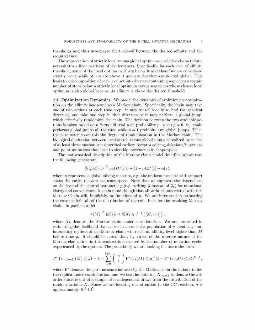
(iv) We estimate Ξ(t) by performing a Taylor expansion of the cumulant ofτ(M) at −∞, yielding

dψ

dξ(logλ) =

∞∑

i=1

ciλi

i!,


100

101

102

103

−101

−100

−10−1

−10−2

−10−3

Number of generations (t)

Ξ(t)

Figure 1. Approximation scheme for Ξ(t) as tց 0+ (incidentally,for this example, E∗[τ ] = 16, 473)

as λց 0+. Inverting the polynomial on the right-hand side we obtain thegeneral approximation form

Ξ(t) ∼= −t−1,

which holds remarkably well as long t ≥ 10, i.e. at least ten generations.For t = 1, 2, . . . , 9 we evaluate Ξ(t) numerically, by solving the associatedpolynomial. Figure 1 shows an example of this approximation scheme.

2.5. Note on random variables. Three distinct sources of randomization play acentral role in our model. In an effort to allay confusion, we want to be particularlyclear about our use of random variables in the description of our results.

Firstly, there is a dimension of randomness arising fundamentally from the ran-dom nature of the mutations during the immune maturation process. We refer todifferent instances of this process as “mutation scenarios” and usually we reservethe letter ω to signify them. The parameter p introduced earlier serves to controlthis dimension of randomness.

Secondly, there is variability within the population of antibodies that make up aparticular germinal center under investigation. We will generally only be concernedwith the proportion of the antibody population from a given germinal center that


shares a common property, rather than the explicit identification of any one anti-body out of the population. Thus, we use the letter q to denote proportions of thispopulation, rather than denoting random elements explicitly.

Thirdly, there is a dimension of randomness arising from the unknown genotypeof the antigenic challenge. As described above, each antigen generates a differentaffinity landscape within which the antibody evolution process occurs. We typicallyreserve the letter z to denote a random instance of an affinity landscape (resultingfrom a random antigen).

As will become apparent in the following sections, our results typically involveproperties of appropriately chosen quantiles of the “response distribution”, i.e. therandom variable measuring the time (in mutation cycles) until a given proportion ofthe antibodies populating the germinal center under investigation reaches an affinityfor the antigen under investigation above a given threshold. Mathematically, theseare quantiles of a stopping time under the probability measure of ω. As such,these objects are still random variables, relative to the choice of a random antigenand resulting affinity landscape z. Later we proceed to describe properties of theresponse distribution relative to randomly chosen antigens. Mathematically, theseare quantiles with respect to the probability measure of z.

We generally use analytic estimates to study the properties of the distributionof ω while reserving simulation techniques for the properties of the distribution ofz. For instance, Figures 2 and 3 are generated analytically, while Figures 4, 5 and6 are generated by repeating the analytical estimates for 1,000 randomly generatedaffinity landscapes.

3. Overview of Results

The setting described above was used in [TT99] to obtain estimates on the re-sponse characteristics of the immune system and its sensitivity to the amount ofmixing in the MC. More concretely, let L(a, b, c) denote the set of affinity land-scapes, parameterized by

• the maximum number of affinity level sets a in a strictly local maximumhill,

• the maximum number of affinity level sets b in a global maximum hill, and• the ratio c of the size of the affinity level sets that belong to the attraction

basin of a strictly local maximum versus those that belong to the globalmaximum attraction basin.

Also, let τ (ω, z, p, q) denote the random number of mutations that it takes undermutation scenario ω for a proportion q of the population of antibodies in a particularGC to reach the desired level set in the random affinity landscape z ∈ L(a, b, c)for some a, b and c, while performing global jumps with probability 1 − p. Thisis a generalization of the stopping time τ(M) defined earlier in the section onOptimization Dynamics. We now suppress the dependence of the stopping time onthe affinity threshold M , focusing instead on the other variables that influence it.We can summarize the results of [TT99] as follows:

(1) For a population N of a few tens of thousands and biologically justifiablevalues of a, b and c (see for example [Elg96, Man90, SM99]), for any p abovesome minimum value and for all z, Pr

(

τ(

·, z, p,N−1)

≤ y)

exhibits a sharpcutoff [OP97]


(2) Let R (c1, z, p, q) denote the c1-quantile of the distribution of τ . Then, forany choice of c1 and for all z, R

(

c1, z, ·, N−1)

exhibits a unique minimumat a p∗ < 1.

(3) The graph of the mean and standard deviation of R(

c1, ·, p,N−1)

overrandomly generated landscapes has two branches, one for low p and one forhigh p, that we designate “liquid” and “solid” state respectively.

(4) Let us begin the MC with a randomly chosen value of p and allow p toevolve taking incremental steps after each antigenic response, with a biastowards the direction of the optimal value of p for the most-recently resolvedantigenic affinity landscape. Under these conditions, the value of p evolvesautonomously to a narrow range (strictly less than 1) around the optimalvalues of the majority of affinity landscapes (“optimal range”).

What we aim in the current paper is to explore three of these areas in moredetail. Specifically, we first investigate how the cutoff behavior changes when werequire that q > N−1. We then attempt to better describe the characteristics ofour conjectured phase transition when we contrast the responses of high-p vs. low-p MCs across randomly generated landscapes. Finally, we define a more realisticversion of the evolving p model and show that the system continues to converge toa value of p in the optimal range.

4. Evolving Population of Antibodies

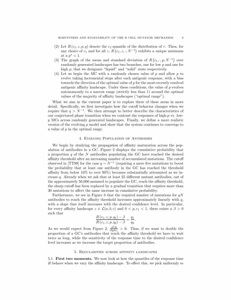
We begin by studying the propagation of affinity maturation across the pop-ulation of antibodies in a GC. Figure 2 displays the cumulative probability thata proportion q of the N antibodies populating the GC have reached the desiredaffinity threshold after an increasing number of accumulated mutations. The cutoffobserved in [TT99] for the case q = N−1 (requiring a mere five mutations to boostthe probability that at least one antibody in the GC has reached the thresholdaffinity from below 10% to over 90%) becomes substantially attenuated as we in-crease q. Already when we ask that at least 25 different mutant antibodies, out ofthe approximately 50,000 assumed to populate the GC, reach the affinity threshold,the sharp cutoff has been replaced by a gradual transition that requires more than30 mutations to affect the same increase in cumulative probability.

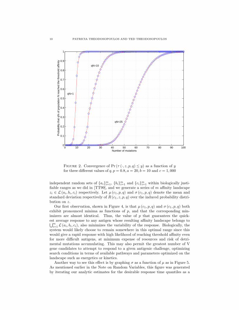
Furthermore, we see in Figure 3 that the required number of mutations for qNantibodies to reach the affinity threshold increases approximately linearly with q,with a slope that itself increases with the desired confidence level. In particular,for every affinity landscape z ∈ L(a, b, c) and 0 < p, c1 < 1, there exists a β > 0such that

R (c1, z, p, q1) − β

R (c1, z, p, q2) − β=q1

q2.

As we would expect from Figure 2, ∂2R∂q∂c1

> 0. Thus, if we want to double the

proportion of a GC’s antibodies that reach the affinity threshold we have to waittwice as long, while the sensitivity of the response time to the desired confidencelevel increases as we increase the target proportion of antibodies.

5. Regularities across affinity landscapes

5.1. First two moments. We now look at how the quantiles of the response timeR behave when we vary the affinity landscape. To effect this, we pick uniformly m


0 10 20 30 40 50 60 70 80 90 1000

0.1

0.2

0.3

0.4

0.5

0.6

0.7

0.8

0.9

1

qN=1

qN=10

qN=25

Number of mutations

Pro

babi

lity

that

q%

of p

opul

atio

n N

rea

ched

the

thre

shol

d af

finity

Figure 2. Convergence of Pr (τ (·, z, p, q) ≤ y) as a function of yfor three different values of q, p = 0.8, a = 20, b = 10 and c = 1, 000

independent random sets of {ai}mi=1, {bi}

mi=1 and {ci}m

i=1 within biologically justi-fiable ranges as we did in [TT99], and we generate a series of m affinity landscapezi ∈ L (ai, bi, ci) respectively. Let µ (c1, p, q) and σ (c1, p, q) denote the mean andstandard deviation respectively of R (c1, z, p, q) over the induced probability distri-bution on z.

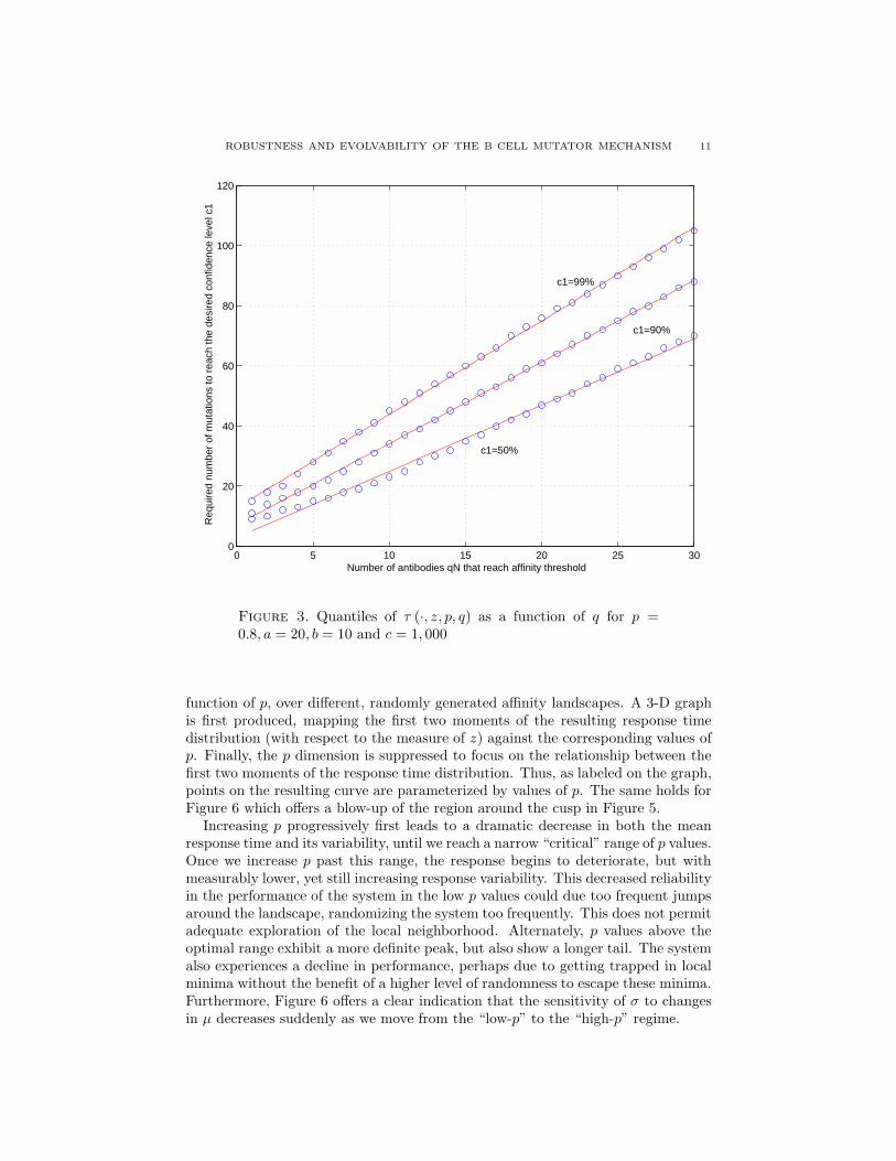
Our first observation, shown in Figure 4, is that µ (c1, p, q) and σ (c1, p, q) bothexhibit pronounced minima as functions of p, and that the corresponding min-imizers are almost identical. Thus, the value of p that guarantees the quick-est average response to any antigen whose resulting affinity landscape belongs to⋃m

i=1 L (ai, bi, ci), also minimizes the variability of the response. Biologically, thesystem would likely choose to remain somewhere in this optimal range since thiswould give a rapid response with high likelihood of reaching threshold affinity evenfor more difficult antigens, at minimum expense of resources and risk of detri-mental mutations accumulating. This may also permit the greatest number of Vgene candidates to attempt to respond to a given antigenic challenge, optimizingsearch conditions in terms of available pathways and parameters optimized on thelandscape such as energetics or kinetics.

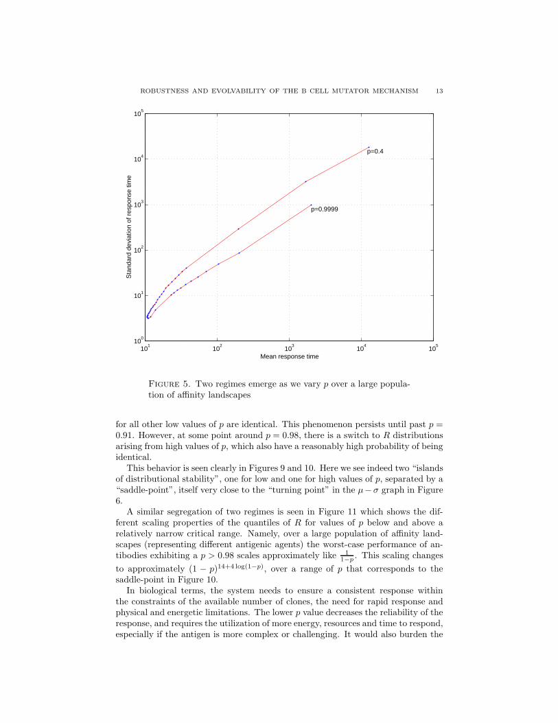
Another way to see this effect is by graphing σ as a function of µ as in Figure 5.As mentioned earlier in the Note on Random Variables, this figure was generatedby iterating our analytic estimates for the desirable response time quantiles as a


0 5 10 15 20 25 300

20

40

60

80

100

120

c1=50%

c1=90%

c1=99%

Number of antibodies qN that reach affinity threshold

Req

uire

d nu

mbe

r of

mut

atio

ns to

rea

ch th

e de

sire

d co

nfid

ence

leve

l c1

Figure 3. Quantiles of τ (·, z, p, q) as a function of q for p =0.8, a = 20, b = 10 and c = 1, 000

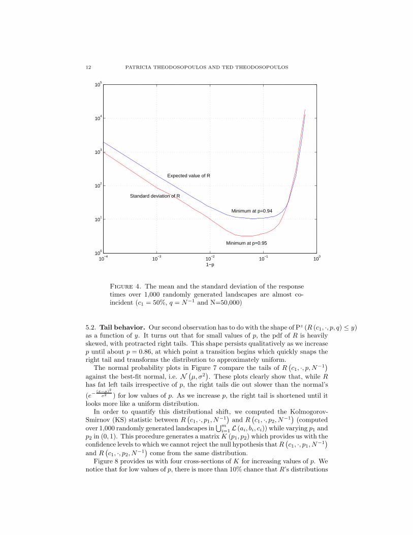
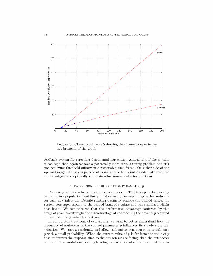
function of p, over different, randomly generated affinity landscapes. A 3-D graphis first produced, mapping the first two moments of the resulting response timedistribution (with respect to the measure of z) against the corresponding values ofp. Finally, the p dimension is suppressed to focus on the relationship between thefirst two moments of the response time distribution. Thus, as labeled on the graph,points on the resulting curve are parameterized by values of p. The same holds forFigure 6 which offers a blow-up of the region around the cusp in Figure 5.

Increasing p progressively first leads to a dramatic decrease in both the meanresponse time and its variability, until we reach a narrow “critical” range of p values.Once we increase p past this range, the response begins to deteriorate, but withmeasurably lower, yet still increasing response variability. This decreased reliabilityin the performance of the system in the low p values could due too frequent jumpsaround the landscape, randomizing the system too frequently. This does not permitadequate exploration of the local neighborhood. Alternately, p values above theoptimal range exhibit a more definite peak, but also show a longer tail. The systemalso experiences a decline in performance, perhaps due to getting trapped in localminima without the benefit of a higher level of randomness to escape these minima.Furthermore, Figure 6 offers a clear indication that the sensitivity of σ to changesin µ decreases suddenly as we move from the “low-p” to the “high-p” regime.


10−4

10−3

10−2

10−1

100

100

101

102

103

104

105

1−p

Expected value of R

Standard deviation of R

Minimum at p=0.95

Minimum at p=0.94

Figure 4. The mean and the standard deviation of the responsetimes over 1,000 randomly generated landscapes are almost co-incident (c1 = 50%, q = N−1 and N=50,000)

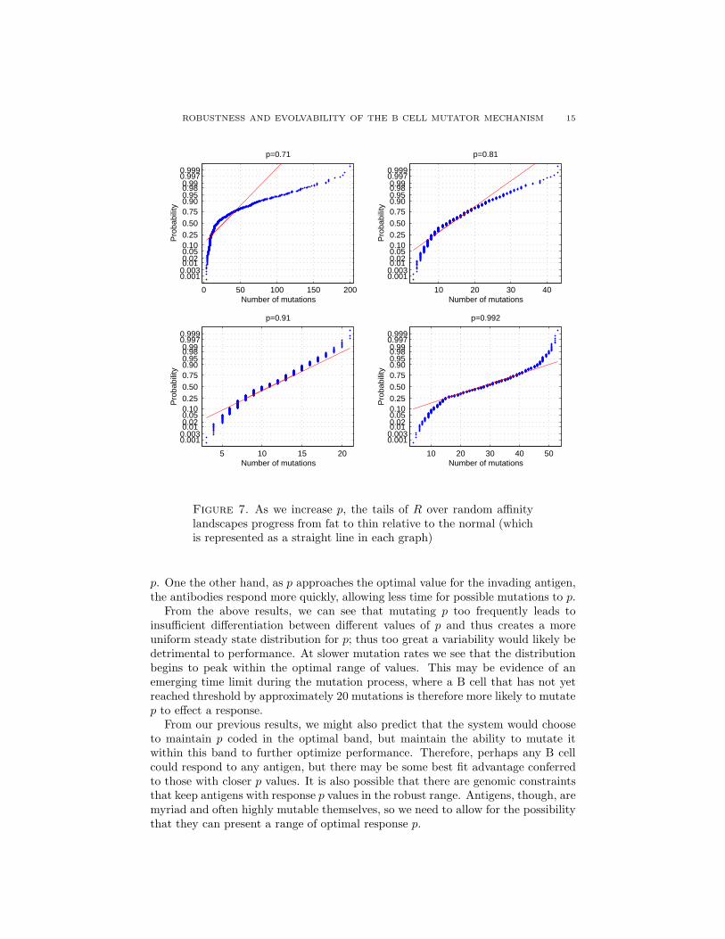
5.2. Tail behavior. Our second observation has to do with the shape of Pz (R (c1, ·, p, q) ≤ y)as a function of y. It turns out that for small values of p, the pdf of R is heavilyskewed, with protracted right tails. This shape persists qualitatively as we increasep until about p = 0.86, at which point a transition begins which quickly snaps theright tail and transforms the distribution to approximately uniform.

The normal probability plots in Figure 7 compare the tails of R(

c1, ·, p,N−1)

against the best-fit normal, i.e. N(

µ, σ2)

. These plots clearly show that, while Rhas fat left tails irrespective of p, the right tails die out slower than the normal’s

(e−(x−µ)2

σ2 ) for low values of p. As we increase p, the right tail is shortened until itlooks more like a uniform distribution.

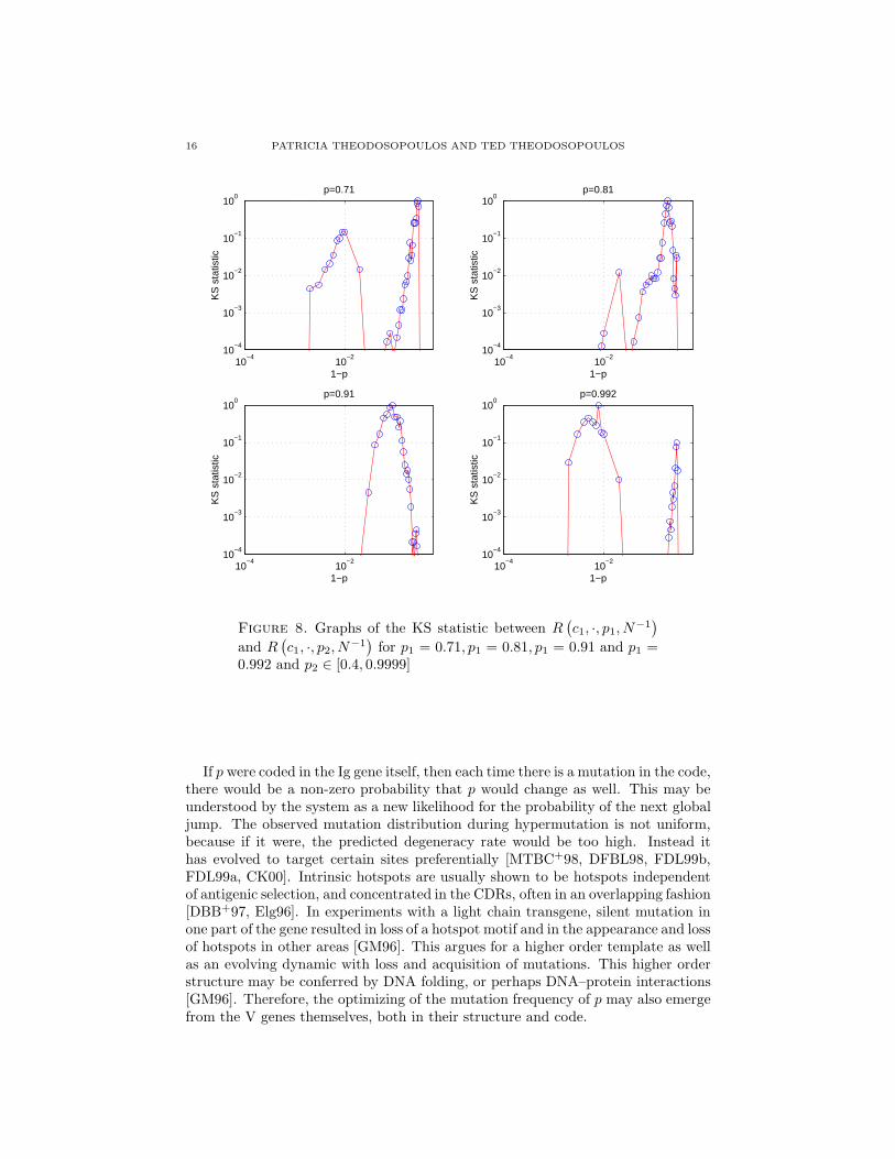
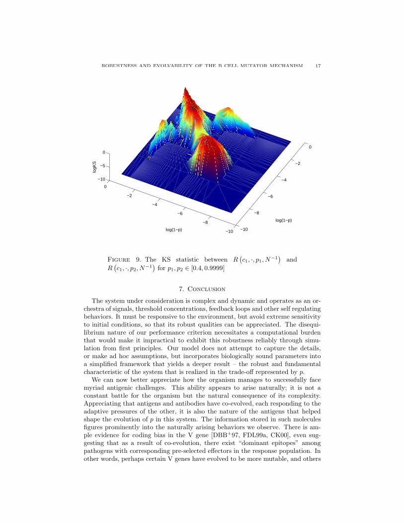
In order to quantify this distributional shift, we computed the Kolmogorov-Smirnov (KS) statistic between R

(

c1, ·, p1, N−1

)

and R(

c1, ·, p2, N−1

)

(computed

over 1,000 randomly generated landscapes in⋃m

i=1 L (ai, bi, ci)) while varying p1 andp2 in (0, 1). This procedure generates a matrixK (p1, p2) which provides us with theconfidence levels to which we cannot reject the null hypothesis thatR

(

c1, ·, p1, N−1

)

and R(

c1, ·, p2, N−1

)

come from the same distribution.Figure 8 provides us with four cross-sections of K for increasing values of p. We

notice that for low values of p, there is more than 10% chance that R’s distributions


101

102

103

104

105

100

101

102

103

104

105

Mean response time

Sta

ndar

d de

viat

ion

of r

espo

nse

time

p=0.9999

p=0.4

Figure 5. Two regimes emerge as we vary p over a large popula-tion of affinity landscapes

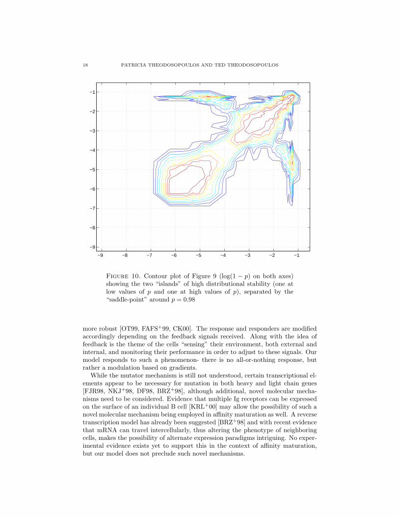
for all other low values of p are identical. This phenomenon persists until past p =0.91. However, at some point around p = 0.98, there is a switch to R distributionsarising from high values of p, which also have a reasonably high probability of beingidentical.

This behavior is seen clearly in Figures 9 and 10. Here we see indeed two “islandsof distributional stability”, one for low and one for high values of p, separated by a“saddle-point”, itself very close to the “turning point” in the µ−σ graph in Figure6.

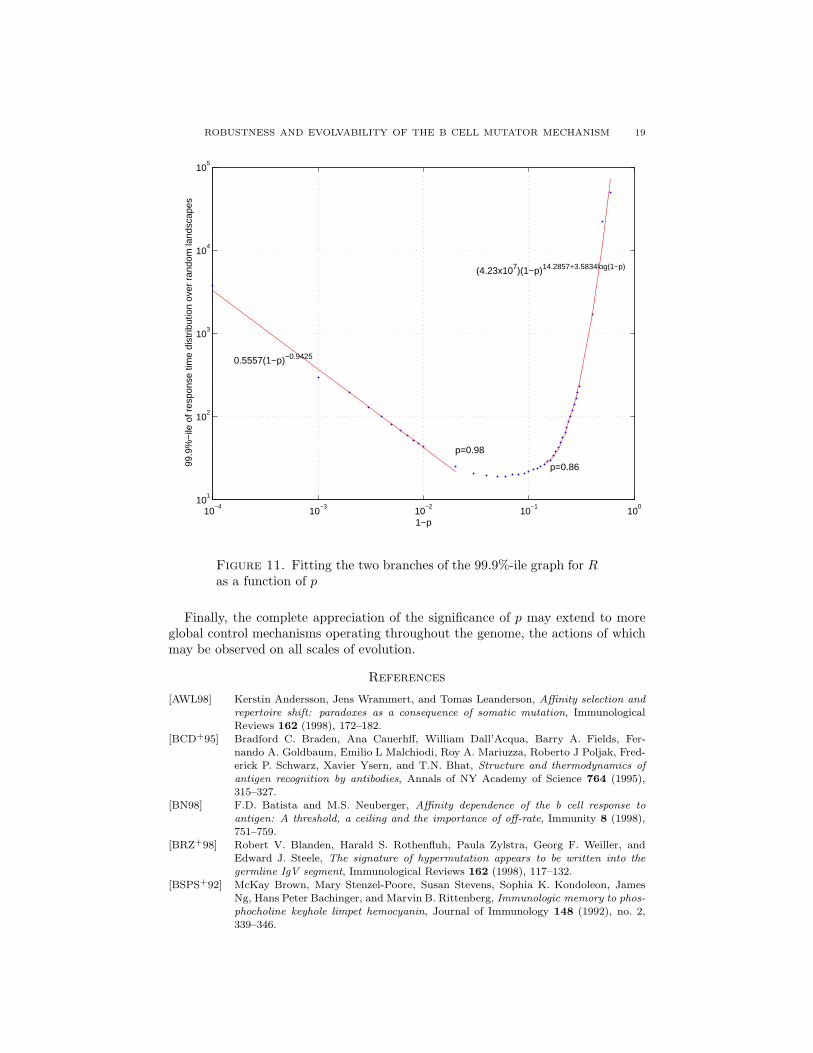
A similar segregation of two regimes is seen in Figure 11 which shows the dif-ferent scaling properties of the quantiles of R for values of p below and above arelatively narrow critical range. Namely, over a large population of affinity land-scapes (representing different antigenic agents) the worst-case performance of an-tibodies exhibiting a p > 0.98 scales approximately like 1

1−p. This scaling changes

to approximately (1 − p)14+4 log(1−p), over a range of p that corresponds to thesaddle-point in Figure 10.

In biological terms, the system needs to ensure a consistent response withinthe constraints of the available number of clones, the need for rapid response andphysical and energetic limitations. The lower p value decreases the reliability of theresponse, and requires the utilization of more energy, resources and time to respond,especially if the antigen is more complex or challenging. It would also burden the


0 20 40 60 80 100 120 140 160 180 2000

50

100

150

200

250

300

Mean response time

Sta

ndar

d de

viat

ion

of r

espo

nse

time

p=0.999

p=0.6

Figure 6. Close-up of Figure 5 showing the different slopes in thetwo branches of the graph

feedback system for screening detrimental mutations. Alternately, if the p valueis too high then again we face a potentially more serious timing problem and risknot achieving threshold affinity in a reasonable time frame. On either side of theoptimal range, the risk is present of being unable to mount an adequate responseto the antigen and optimally stimulate other immune effector functions.

6. Evolution of the control parameter p

Previously we used a hierarchical evolution model [TT99] to depict the evolvingvalue of p in a population, and the optimal value of p corresponding to the landscapefor each new infection. Despite starting distinctly outside the desired range, thesystem converged rapidly to the desired band of p values and was stabilized withinthat band. We hypothesized that the performance advantage conferred by thisrange of p values outweighed the disadvantage of not reaching the optimal p requiredto respond to any individual antigen.

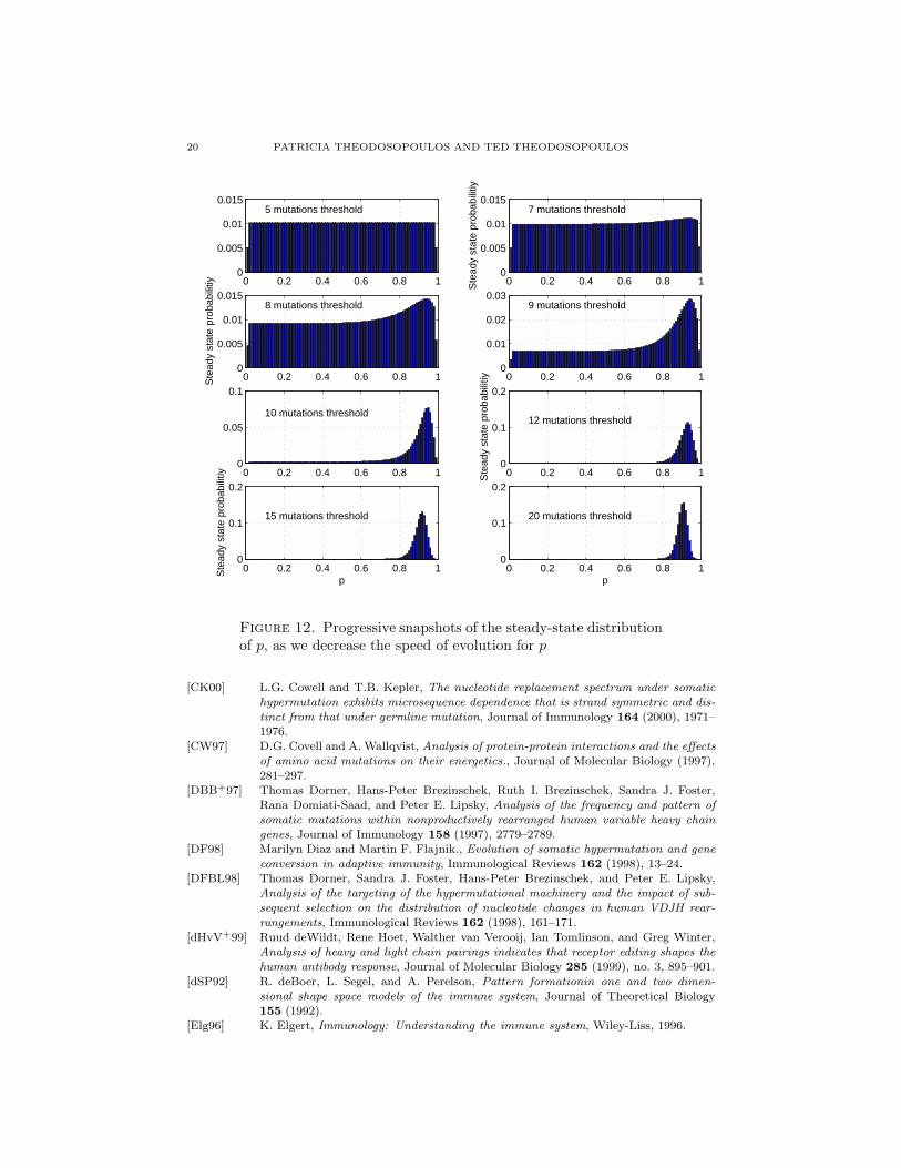
In our current treatment of evolvability, we want to better understand how thefrequency of mutations in the control parameter p influences its steady-state dis-tribution. We start p randomly, and allow each subsequent mutation to influencep with a small probability. When the current value of p is far from the value of pthat minimizes the response time to the antigen we are facing, then the antibodieswill need more mutations, leading to a higher likelihood of an eventual mutation in


0 50 100 150 200

0.0010.0030.01 0.02 0.05 0.10 0.25 0.50 0.75 0.90 0.95 0.98 0.99

0.9970.999

Number of mutations

Pro

babi

lity

p=0.71

10 20 30 40

0.0010.0030.01 0.02 0.05 0.10 0.25 0.50 0.75 0.90 0.95 0.98 0.99

0.9970.999

Number of mutations

Pro

babi

lity

p=0.81

5 10 15 20

0.0010.0030.01 0.02 0.05 0.10 0.25 0.50 0.75 0.90 0.95 0.98 0.99

0.9970.999

Number of mutations

Pro

babi

lity

p=0.91

10 20 30 40 50

0.0010.0030.01 0.02 0.05 0.10 0.25 0.50 0.75 0.90 0.95 0.98 0.99

0.9970.999

Number of mutations

Pro

babi

lity

p=0.992

Figure 7. As we increase p, the tails of R over random affinitylandscapes progress from fat to thin relative to the normal (whichis represented as a straight line in each graph)

p. One the other hand, as p approaches the optimal value for the invading antigen,the antibodies respond more quickly, allowing less time for possible mutations to p.

From the above results, we can see that mutating p too frequently leads toinsufficient differentiation between different values of p and thus creates a moreuniform steady state distribution for p; thus too great a variability would likely bedetrimental to performance. At slower mutation rates we see that the distributionbegins to peak within the optimal range of values. This may be evidence of anemerging time limit during the mutation process, where a B cell that has not yetreached threshold by approximately 20 mutations is therefore more likely to mutatep to effect a response.

From our previous results, we might also predict that the system would chooseto maintain p coded in the optimal band, but maintain the ability to mutate itwithin this band to further optimize performance. Therefore, perhaps any B cellcould respond to any antigen, but there may be some best fit advantage conferredto those with closer p values. It is also possible that there are genomic constraintsthat keep antigens with response p values in the robust range. Antigens, though, aremyriad and often highly mutable themselves, so we need to allow for the possibilitythat they can present a range of optimal response p.


10−4

10−2

10−4

10−3

10−2

10−1

100

1−p

KS

sta

tistic

p=0.71

10−4

10−2

10−4

10−3

10−2

10−1

100

1−p

KS

sta

tistic

p=0.81

10−4

10−2

10−4

10−3

10−2

10−1

100

1−p

KS

sta

tistic

p=0.91

10−4

10−2

10−4

10−3

10−2

10−1

100

1−p

KS

sta

tistic

p=0.992

Figure 8. Graphs of the KS statistic between R(

c1, ·, p1, N−1

)

and R(

c1, ·, p2, N−1

)

for p1 = 0.71, p1 = 0.81, p1 = 0.91 and p1 =0.992 and p2 ∈ [0.4, 0.9999]

If p were coded in the Ig gene itself, then each time there is a mutation in the code,there would be a non-zero probability that p would change as well. This may beunderstood by the system as a new likelihood for the probability of the next globaljump. The observed mutation distribution during hypermutation is not uniform,because if it were, the predicted degeneracy rate would be too high. Instead ithas evolved to target certain sites preferentially [MTBC+98, DFBL98, FDL99b,FDL99a, CK00]. Intrinsic hotspots are usually shown to be hotspots independentof antigenic selection, and concentrated in the CDRs, often in an overlapping fashion[DBB+97, Elg96]. In experiments with a light chain transgene, silent mutation inone part of the gene resulted in loss of a hotspot motif and in the appearance and lossof hotspots in other areas [GM96]. This argues for a higher order template as wellas an evolving dynamic with loss and acquisition of mutations. This higher orderstructure may be conferred by DNA folding, or perhaps DNA–protein interactions[GM96]. Therefore, the optimizing of the mutation frequency of p may also emergefrom the V genes themselves, both in their structure and code.


−10

−8

−6

−4

−2

0

−10

−8

−6

−4

−2

0

−10

−5

0

log(1−p)

log(1−p)

logK

S

Figure 9. The KS statistic between R(

c1, ·, p1, N−1

)

and

R(

c1, ·, p2, N−1

)

for p1, p2 ∈ [0.4, 0.9999]

7. Conclusion

The system under consideration is complex and dynamic and operates as an or-chestra of signals, threshold concentrations, feedback loops and other self regulatingbehaviors. It must be responsive to the environment, but avoid extreme sensitivityto initial conditions, so that its robust qualities can be appreciated. The disequi-librium nature of our performance criterion necessitates a computational burdenthat would make it impractical to exhibit this robustness reliably through simu-lation from first principles. Our model does not attempt to capture the details,or make ad hoc assumptions, but incorporates biologically sound parameters intoa simplified framework that yields a deeper result – the robust and fundamentalcharacteristic of the system that is realized in the trade-off represented by p.

We can now better appreciate how the organism manages to successfully facemyriad antigenic challenges. This ability appears to arise naturally; it is not aconstant battle for the organism but the natural consequence of its complexity.Appreciating that antigens and antibodies have co-evolved, each responding to theadaptive pressures of the other, it is also the nature of the antigens that helpedshape the evolution of p in this system. The information stored in such moleculesfigures prominently into the naturally arising behaviors we observe. There is am-ple evidence for coding bias in the V gene [DBB+97, FDL99a, CK00], even sug-gesting that as a result of co-evolution, there exist “dominant epitopes” amongpathogens with corresponding pre-selected effectors in the response population. Inother words, perhaps certain V genes have evolved to be more mutable, and others


−9 −8 −7 −6 −5 −4 −3 −2 −1

−9

−8

−7

−6

−5

−4

−3

−2

−1

Figure 10. Contour plot of Figure 9 (log(1 − p) on both axes)showing the two “islands” of high distributional stability (one atlow values of p and one at high values of p), separated by the“saddle-point” around p = 0.98

more robust [OT99, FAFS+99, CK00]. The response and responders are modifiedaccordingly depending on the feedback signals received. Along with the idea offeedback is the theme of the cells “sensing” their environment, both external andinternal, and monitoring their performance in order to adjust to these signals. Ourmodel responds to such a phenomenon- there is no all-or-nothing response, butrather a modulation based on gradients.

While the mutator mechanism is still not understood, certain transcriptional el-ements appear to be necessary for mutation in both heavy and light chain genes[FJR98, NKJ+98, DF98, BRZ+98], although additional, novel molecular mecha-nisms need to be considered. Evidence that multiple Ig receptors can be expressedon the surface of an individual B cell [KRL+00] may allow the possibility of such anovel molecular mechanism being employed in affinity maturation as well. A reversetranscription model has already been suggested [BRZ+98] and with recent evidencethat mRNA can travel intercellularly, thus altering the phenotype of neighboringcells, makes the possibility of alternate expression paradigms intriguing. No exper-imental evidence exists yet to support this in the context of affinity maturation,but our model does not preclude such novel mechanisms.


10−4

10−3

10−2

10−1

100

101

102

103

104

105

1−p

99.9

%−

ile o

f res

pons

e tim

e di

strib

utio

n ov

er r

ando

m la

ndsc

apes

0.5557(1−p)−0.9425

(4.23x107)(1−p)14.2857+3.5834log(1−p)

p=0.98

p=0.86

Figure 11. Fitting the two branches of the 99.9%-ile graph for Ras a function of p

Finally, the complete appreciation of the significance of p may extend to moreglobal control mechanisms operating throughout the genome, the actions of whichmay be observed on all scales of evolution.

References

[AWL98] Kerstin Andersson, Jens Wrammert, and Tomas Leanderson, Affinity selection and

repertoire shift: paradoxes as a consequence of somatic mutation, ImmunologicalReviews 162 (1998), 172–182.

[BCD+95] Bradford C. Braden, Ana Cauerhff, William Dall’Acqua, Barry A. Fields, Fer-nando A. Goldbaum, Emilio L Malchiodi, Roy A. Mariuzza, Roberto J Poljak, Fred-erick P. Schwarz, Xavier Ysern, and T.N. Bhat, Structure and thermodynamics of

antigen recognition by antibodies, Annals of NY Academy of Science 764 (1995),315–327.

[BN98] F.D. Batista and M.S. Neuberger, Affinity dependence of the b cell response to

antigen: A threshold, a ceiling and the importance of off-rate, Immunity 8 (1998),751–759.

[BRZ+98] Robert V. Blanden, Harald S. Rothenfluh, Paula Zylstra, Georg F. Weiller, andEdward J. Steele, The signature of hypermutation appears to be written into the

germline IgV segment, Immunological Reviews 162 (1998), 117–132.

[BSPS+92] McKay Brown, Mary Stenzel-Poore, Susan Stevens, Sophia K. Kondoleon, JamesNg, Hans Peter Bachinger, and Marvin B. Rittenberg, Immunologic memory to phos-

phocholine keyhole limpet hemocyanin, Journal of Immunology 148 (1992), no. 2,339–346.


0 0.2 0.4 0.6 0.8 10

0.005

0.01

0.0155 mutations threshold

0 0.2 0.4 0.6 0.8 10

0.005

0.01

0.015

Ste

ady

stat

e pr

obab

ilitiy

7 mutations threshold

0 0.2 0.4 0.6 0.8 10

0.005

0.01

0.015

Ste

ady

stat

e pr

obab

ilitiy


0 0.2 0.4 0.6 0.8 10

0.01

0.02

0.039 mutations threshold

0 0.2 0.4 0.6 0.8 10

0.05

0.1


0 0.2 0.4 0.6 0.8 10

0.1

0.2

Ste

ady

stat

e pr

obab

ilitiy


0 0.2 0.4 0.6 0.8 10

0.1

0.2

p

Ste

ady

stat

e pr

obab

ilitiy


0 0.2 0.4 0.6 0.8 10

0.1

0.2

p


Figure 12. Progressive snapshots of the steady-state distributionof p, as we decrease the speed of evolution for p

[CK00] L.G. Cowell and T.B. Kepler, The nucleotide replacement spectrum under somatic

hypermutation exhibits microsequence dependence that is strand symmetric and dis-

tinct from that under germline mutation, Journal of Immunology 164 (2000), 1971–1976.

[CW97] D.G. Covell and A. Wallqvist, Analysis of protein-protein interactions and the effects

of amino acid mutations on their energetics., Journal of Molecular Biology (1997),281–297.

[DBB+97] Thomas Dorner, Hans-Peter Brezinschek, Ruth I. Brezinschek, Sandra J. Foster,Rana Domiati-Saad, and Peter E. Lipsky, Analysis of the frequency and pattern of

somatic mutations within nonproductively rearranged human variable heavy chain

genes, Journal of Immunology 158 (1997), 2779–2789.[DF98] Marilyn Diaz and Martin F. Flajnik., Evolution of somatic hypermutation and gene

conversion in adaptive immunity, Immunological Reviews 162 (1998), 13–24.[DFBL98] Thomas Dorner, Sandra J. Foster, Hans-Peter Brezinschek, and Peter E. Lipsky,

Analysis of the targeting of the hypermutational machinery and the impact of sub-

sequent selection on the distribution of nucleotide changes in human VDJH rear-

rangements, Immunological Reviews 162 (1998), 161–171.[dHvV+99] Ruud deWildt, Rene Hoet, Walther van Verooij, Ian Tomlinson, and Greg Winter,

Analysis of heavy and light chain pairings indicates that receptor editing shapes the

human antibody response, Journal of Molecular Biology 285 (1999), no. 3, 895–901.

[dSP92] R. deBoer, L. Segel, and A. Perelson, Pattern formationin one and two dimen-

sional shape space models of the immune system, Journal of Theoretical Biology155 (1992).

[Elg96] K. Elgert, Immunology: Understanding the immune system, Wiley-Liss, 1996.


[FAFS+99] K. Furukawa, A. Atsuke-Furukawa, H. Shirai, H. Nakamura, and T. Azuma, Junc-

tional amino acids determine the maturation pathway of an antibody, Immunity 11

(1999), 329–338.[FDL99a] Sandra J. Foster, Thomas Dorner, and Peter E. Lipsky, Somatic hypermutation of

vkjk rearrangements: targeting of rgyw motifs on both dna strands and preferential

selection of mutated codons within rgyw motifs, European Journal of Immunology29 (1999), 4011–4021.

[FDL99b] S.J. Foster, T. Dorner, and P.E. Lipsky, Targeting and subsequent selection of so-

matic hypermutations in the human vk repertoire, European Journal of Immunology29 (1999), 3122–3132.

[FJR98] Y. Fukita, H. Jacobs, and K. Rajewsky, Somatic hypermutation in the heavy chain

locus correlates with transcription, Immunity 9 (1998), 105–114.[FM91] Jefferson Foote and Cesar Milstein, Kinetic maturation of an immune response,

Nature 352 (1991), 530–532.[GEBL98] P. Guermonprez, P. England, H. Bedoulle, and C. Leclerc, The rate of dissociation

between antibody and antigen determines the efficiency of antibody-mediated antigen

presentation, Journal of Immunology 161 (1998), 4542–4548.[GM96] Beatriz Goyenechea and Cesar Milstein, Modifying the sequence of an immunoglob-

ulin V gene alters the resulting pattern of hypermutation, Immunology 93 (1996),

13979–13984.[HSF96] M.A. Huynen, P.F. Stadler, and W. Fontana, Smoothness within ruggedness: The

role of neutrality in adaption, Proceedings of the National Academy of Sciences 93

(1996), 397–401.[JMS+95] Harry W. Schroeder Jr, Frank Mortari, Satoshi Shiokawa, Perry Kirkham, Rotem A.

Elgavish, and F.E. Bertrand III, Developmental regulation of the human antibody

repertoire, Annals of NY Acad. of Science (1995), 242–260.[KGF+98] Ulf Klein, Tina Goossens, Matthias Fischer, Holger Kanzler, Andreas Braeuninger,

Klaus Rajewsky, and Ralf Kuppers, Somatic hypermutation in normal and trans-

formed B cells, Immunological Reviews 162 (1998), 261–280.[KRL+00] J.J. Kenny, L.J. Reznaka, A. Lustig, R.T. Fischer, J. Yoder, S. Marshall, and D.L.

Longo, Autoreactive b cells escape clonal deletion by expressing multiple antigen

receptors, Journal of Immunology 164 (2000), 4111–4119.[Man90] Tim Manser, The efficiency of antibody affinity maturation: can the rate of B-cell

division be limiting, Immunology Today 11 (1990), no. 9, 305–308.[MTBC+98] Tim Manser, Kathleen M. Tumas-Brundage, Lawrence P. Casson, Angela M. Giusti,

Shailaja Hande, Evangelia Notidis, and Kalpit A. Vora, The roles of antibody vari-

able region hypermutation and selection in the development of the memory B cell

compartment, Immunological Reviews 162 (1998), 182–196.[NKJ+98] M. Neuberger, Norman Klix, Christopher J. Jolly, Jose Yelamos, Cristina Rada,

and Cesar Milstein, The intrinsic features of somatic hypermutation, ImmunologicalReviews 162 (1998), 107–116.

[Nos92] G.J.V. Nossal, The molecular and cellular basis of affinity maturation in the antibody

response, Cell 68 (1992), 1–2.[NTM+98] B. Nayak, R. Tuteja, V. Manivel, R.P. Roy, R.A. Vishwakarma, and K.V.S. Rao, B

cell responses to a peptide epitope v. kinetic regulation of repertoire discrimination

and antibody optimization for epitope, Journal of Immunology 161 (1998), 3510–3519.

[OP97] Mihaela Oprea and Alan S. Perelson, Somatic mutation leads to efficient affinity

maturation when centrocytes recycle back to centroblasts, Journal of Immunology158 (1997), 5155–5162.

[OT99] M. Oprea and T.B.Kepler, Somatic hypermutation: statistical analyses using a new

resampling based methodology, Genome Research 12 (1999), 1294–1304.[PO79] A. Perelson and G. Oster, Theoretical studies of clonal selection: Minimal antibody

repertoire size and reliability of self-non-self discrimination, Journal of TheoreticalBiology 81 (1979).

[Row94] G.W. Rowe, Theoretical models in biology, Oxford University Press, 1994.


[SM99] Michele Shannon and Ramit Mehr, Reconciling repertoire shift with affinity matu-

ration: the role of deleterious mutations, Journal of Immunology 162 (1999), no. 7,3950–3956.

[The95] T.V. Theodosopoulos, Stochastic models for global optimization, Tech. Report LIDS- TH - 2323, Laboratory for Information and Decision Systems, MIT, May 1995.

[The99] , Some remarks on the optimal level of randomization in global optimization,Randomization Methods in Algorithm Design (P.M. Pardalos, S. Rajasekaran, andJ. Rolim, eds.), American Mathematical Society, 1999.

[TT99] P.K. Theodosopoulos and T.V. Theodosopoulos, Evolution at the edge of chaos: a

paradigm for the maturation of the humoral immune response, DIMACS Workshopon Evolution as Computation, January 1999.

[WPW+97] Gary J. Wedemayer, Phillip A. Patten, Leo H. Wang, Peter G. Schultz, and Ray-mond C. Stevens, Structural insights into the evolution of an antibody combining

site, Science 276 (1997), no. 5319, 1421–1423.[WRW+98] Gregory D. Wiens, Victoria A. Roberts, Elizabeth A. Whitcomb, Thomas O’Hare,

Mary P. Stenzel-Poore, and Marvin B. Rittenberg, Harmful somatic mutations:

lessons from the dark side, Immunological Reviews 162 (1998), 197–209.

Department of Mathematics and, Department of Decision Sciences, Drexel Univer-

sity, Philadelphia, PA 19066

E-mail address: [email protected]

URL: faculty.lebow.drexel.edu/TheodosopoulosT

Documents

Robustness and Evolvability of the B Cell Mutator Mechanism