Embed Size (px)
Citation preview

NATIONAL OPEN UNIVERSITY OF NIGERIA
SCHOOL OF SCIENCE AND TECHNOLOGY
COURSE CODE: FMT 206
COURSE TITLE: INTRODUCTION TO MATHEMATICAL SOFTWARES
INTRODUCTION TO MATHEMATICAL SOFTWARES
FMT 206
Course Guide
Course Developer/Writer: Mrs. Banjoko Temitope and Dr. Ajibola. S.O
Course Editor: John Erigbe
Programme Leader: Dr. AJIBOLA Saheed. O
School of Science and Technology
National Open University of Nigeria.
Course Coordinator:

CONTENT
Introduction
Course Aim
Course Objectives
Study Units
Assignments
Tutor Marked Assignment
Final Examination and Grading
Summary
INTRODUCTION
You are holding in your hand the course guide for FMT 206 (Introduction to Mathematical softwares). The purpose of the course guide is to relate to you the basic structure of the course material you are expected to study. Like the name ‘course guide’ implies, it is to guide you on what to expect from the course material and at the end of studying the course material.
COURSE CONTENT
The course content consists basically of the introduction to Mathematical softwares like: MATLAB, MAPLE and Ms. Excel softwares packages.
COURSE AIM
The aim of the course is to bring to your cognizance the introduction to Mathematical softwares as mentioned in the course content to handle Finitial problems and calculations.
COURSE OBJECTIVES
At the end of studying the course material, among other objectives, you should be able to:
1. Explain the concepts of soft wares; 2. The use of MATLAB to solve financial Problems; 3. The use of MAPLE to solve financial Problems ; 4. The use of Ms Excel to solve financial Problems;
COURSE MATERIAL
The course material package is composed of: The Course Guide The study units Self-Assessment Exercises Tutor Marked Assignment References/Further Reading
THE STUDY UNITS
The study units are as listed below:
Unit ONE 1.0 What is MATLAB 1.1 A model of price evolution 1.2 Central Limit Theorem 1.3 Geometric Brownian Motion UNIT TWO 2.0 Elementary financial calculations 2.1 Interest rates 2.2 Present value analysis UNIT THREE 3.0 Rate of return 3.1 Pricing via arbitrage 3.2 The multi-period binomial model 3.3 The Black–Scholes formula UNIT FOUR 4.0 SECTIONS A: Overcoming limitations Using MATLAB 4.1 A.1: The program present value 4.2 A.2 The program ror 4. 3 A.3 The program mbm
ASSIGNMENTS
Each unit of the course has a self assessment exercise. You will be expected to attempt them as this will enable you learn the facts of the unit.
TUTOR MARKED ASSIGNMENT
The Tutor Marked Assignments (TMAs) at the end of each unit are designed to test your knowledge and application of the concepts learned. Besides the preparatory TMAs in the course material to test what has been learnt, it is important that you

know that at the end of the course, you must have done your examinable TMAs as they fall due, which are marked electronically. They make up to 30 percent of the total score for the course.
SUMMARY
Financial Mathematics can be compared to a cathedral. We wish to visit a small part of this cathedral of human ideas of quantities and space. We wish to learn how financial mathematics can be built. Financial Mathematics spans a very wide spectrum, from the simple arithmetic operations a pupil learns in primary school to the sophisticated and difficult research which only a specialist can understand after years of long and hard postgraduate study. We place ourselves somewhere higher up in the lower half of this spectrum. This can also be roughly described as where University mathematics starts. In natural sciences, the criterion of validity of a theory is experiment and practice. Financial mathematics is very different. Experiment and practice are insufficient for establishing mathematical truth. Mathematics is deductive, the only means of ascertaining the validity of a statement is logic. However, the chain of logical arguments cannot be extended indefinitely: inevitably there comes a point where we have to accept some basic propositions without proofs. The era which huge and complex calculations take eternity to arrive has passed and technology has made so many things easy for us. Thus, in this course, you will be introduced to three different software: MATLAB, MAPLE and Ms. EXCEL that are being used in financial mathematics to ease your work. Enjoy the course.
It is very important that you commit adequate effort to the study of the course material for maximum benefit and continuous using of the softwares. \
Good luck.
INTRODUCTION TO MATHEMATICAL SOFTWARES
FMT 206
Course Material
Course Developer/Writer: Mrs. Banjoko Temitope and Dr. Ajibola. S.O
Course Editor: John Erigbe
Programme Leader: Dr. AJIBOLA Saheed. O
School of Science and Technology
National Open University of Nigeria.
Course Coordinator:

CONTENT
Introduction
Course Aim
Course Objectives
Study Units
Assignments
Tutor Marked Assignment
Final Examination and Grading
Summary
Unit ONE 3.0 What is MATLAB 1.1 A model of price evolution 1.2 Central Limit Theorem 1.3 Geometric Brownian Motion UNIT TWO 4.0 Elementary financial calculations 2.1 Interest rates 2.2 Present value analysis UNIT THREE 3.0 Rate of return 3.1 Pricing via arbitrage 3.2 The multi-period binomial model 3.3 The Black–Scholes formula UNIT FOUR 4.0 SECTIONS A: Overcoming limitations Using MATLAB 4.1 A.1: The program present_value 4.2 A.2 The program ror 4. 3 A.3 The program mbm Introduction
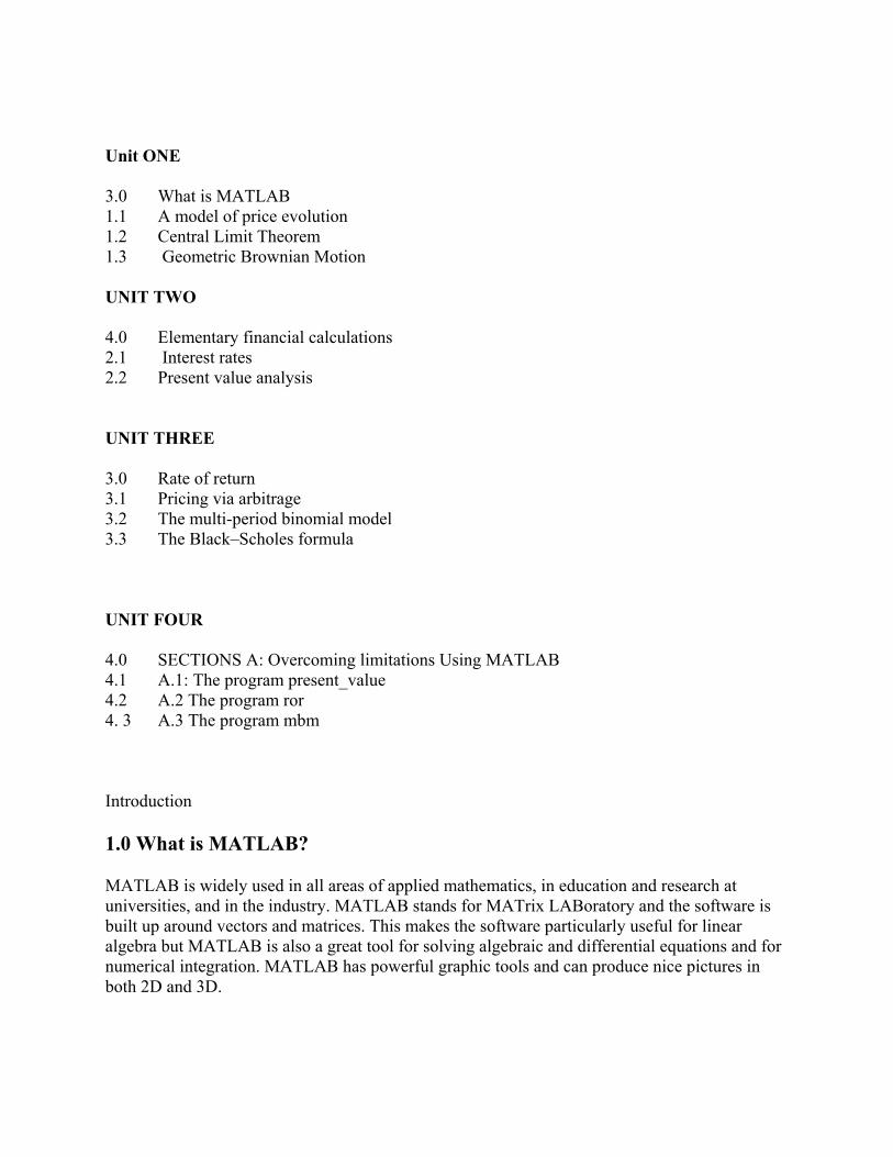
1.0 What is MATLAB?
MATLAB is widely used in all areas of applied mathematics, in education and research at universities, and in the industry. MATLAB stands for MATrix LABoratory and the software is built up around vectors and matrices. This makes the software particularly useful for linear algebra but MATLAB is also a great tool for solving algebraic and differential equations and for numerical integration. MATLAB has powerful graphic tools and can produce nice pictures in both 2D and 3D.
It is also a programming language, and is one of the easiest programming languages for writing mathematical programs. MATLAB also has some tool boxes useful for signal processing, image processing, optimization, etc.
MATLAB is a high performance language for technical computing. It integrates computation, visualisation and programming in an easy-to-use environment where problems and solutions are expressed in familiar mathematical notation. The name MATLAB stands for matrix laboratory.
The best way to learn to use MATLAB is to read this while running MATLAB, trying the examples and experimenting.
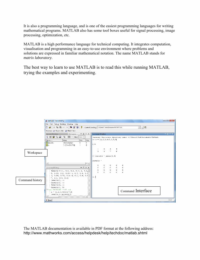
The MATLAB documentation is available in PDF format at the following address: http://www.mathworks.com/access/helpdesk/help/techdoc/matlab.shtml
Workspace
Command history
Command Interface
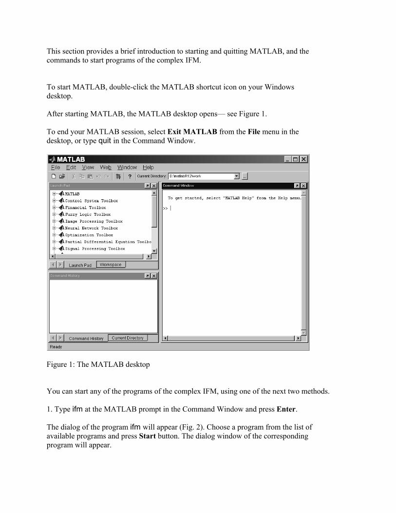
This section provides a brief introduction to starting and quitting MATLAB, and the commands to start programs of the complex IFM. To start MATLAB, double-click the MATLAB shortcut icon on your Windows desktop. After starting MATLAB, the MATLAB desktop opens— see Figure 1. To end your MATLAB session, select Exit MATLAB from the File menu in the desktop, or type quit in the Command Window.
Figure 1: The MATLAB desktop You can start any of the programs of the complex IFM, using one of the next two methods. 1. Type ifm at the MATLAB prompt in the Command Window and press Enter. The dialog of the program ifm will appear (Fig. 2). Choose a program from the list of available programs and press Start button. The dialog window of the corresponding program will appear.
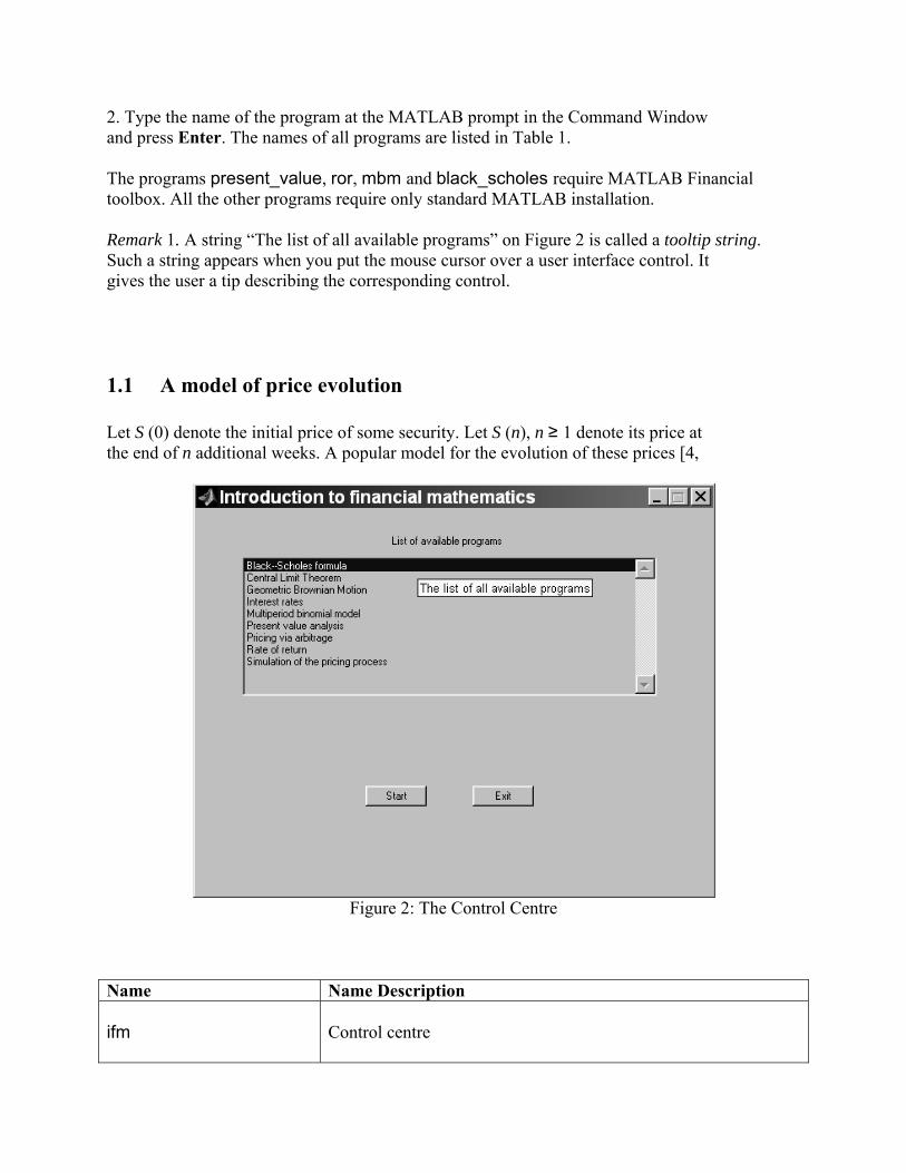
2. Type the name of the program at the MATLAB prompt in the Command Window and press Enter. The names of all programs are listed in Table 1. The programs present_value, ror, mbm and black_scholes require MATLAB Financial toolbox. All the other programs require only standard MATLAB installation. Remark 1. A string “The list of all available programs” on Figure 2 is called a tooltip string. Such a string appears when you put the mouse cursor over a user interface control. It gives the user a tip describing the corresponding control. 1.1 A model of price evolution Let S (0) denote the initial price of some security. Let S (n), n ≥ 1 denote its price at the end of n additional weeks. A popular model for the evolution of these prices [4,
Figure 2: The Control Centre
Name Name Description ifm
Control centre
price evolution
A model of price evolution
clt
An illustration of the Central limit theorem
gbm
Geometric Brownian motion
interest rate
Interest rates
present value
Present value analysis
ror
Rate of return
Options_ pricing
Pricing via arbitrage
mbm
Multiperiod binomial model
black scholes
Black–Scholes formula
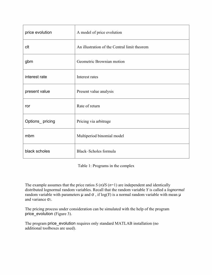
Table 1: Programs in the complex
The example assumes that the price ratios S (n)/S (n−1) are independent and identically distributed lognormal random variables. Recall that the random variable Y is called a lognormal random variable with parameters μ and σ , if log(Y) is a normal random variable with mean μ and variance σ2. The pricing process under consideration can be simulated with the help of the program price_evolution (Figure 3). The program price_evolution requires only standard MATLAB installation (no additional toolboxes are used).
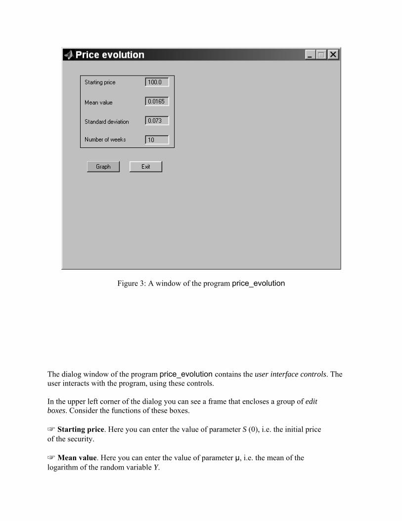
Figure 3: A window of the program price_evolution
The dialog window of the program price_evolution contains the user interface controls. The user interacts with the program, using these controls. In the upper left corner of the dialog you can see a frame that encloses a group of edit boxes. Consider the functions of these boxes. ☞ Starting price. Here you can enter the value of parameter S (0), i.e. the initial price of the security. ☞ Mean value. Here you can enter the value of parameter μ, i.e. the mean of the logarithm of the random variable Y.

☞ Standard deviation. Here you can enter the value of parameter σ, i.e. the standard deviation of the logarithm of the random variable Y. ☞ Number of weeks. Here you can enter the length of the time interval of simulation of the evolution of the price, measured in weeks. Remark 2. Some edit boxes in the programs of the complex have default values. In simple cases, you can start calculations without changing these values. We will refer to this feature as solution of the standard problem. Fig. 3 shows that the standard problem has the following values: starting price is equal to 100 (say, Swedish krones), mean value is equal to 0.0165, standard deviation is equal to 0.073, and we want to simulate price evolution during 10 weeks. Remark 3. Some edit boxes have prevention to non-correct input. For example, somebody tried to enter a negative value of the starting price into the corresponding edit box. The result is shown on Fig. 4. A warning message was produced, and the program returned the previous value into the edit box instead of the wrong value. In such cases, you must press the OK button in order to continue your work.
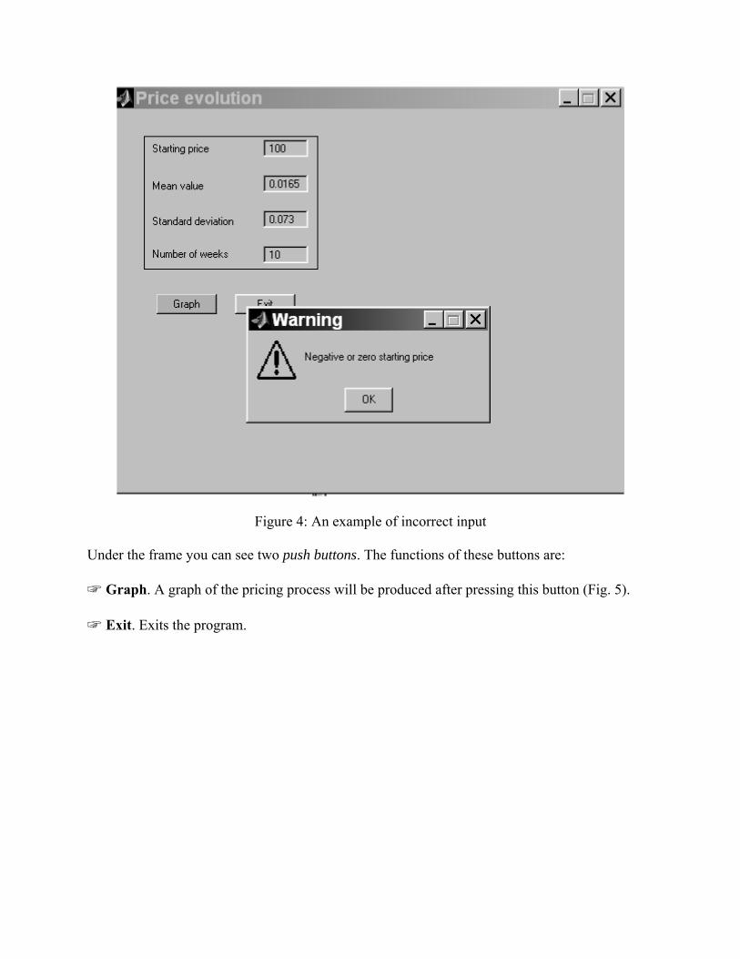
Figure 4: An example of incorrect input
Under the frame you can see two push buttons. The functions of these buttons are: ☞ Graph. A graph of the pricing process will be produced after pressing this button (Fig. 5). ☞ Exit. Exits the program.
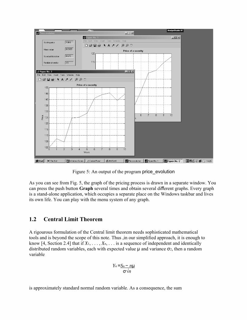
Figure 5: An output of the program price_evolution As you can see from Fig. 5, the graph of the pricing process is drawn in a separate window. You can press the push button Graph several times and obtain several different graphs. Every graph is a stand-alone application, which occupies a separate place on the Windows taskbar and lives its own life. You can play with the menu system of any graph. 1.2 Central Limit Theorem A rigourous formulation of the Central limit theorem needs sophisticated mathematical tools and is beyond the scope of this note. Thus ,in our simplified approach, it is enough to know [4, Section 2.4] that if X1, . . . , Xn, . . . is a sequence of independent and identically distributed random variables, each with expected value μ and variance σ2, then a random variable
Yn =Sn − nμ σ√n
is approximately standard normal random variable. As a consequence, the sum
is approximately a normal random variable with expected value nμ and variance nσ2. Consider the following example: Let X1 be a Bernoulli random variable, i.e., X1 = 1 with probability p and X1 = 0 with probability 1 − p. EX1 = p, Var X1 = p(1 − p). According to the central limit theorem, a random variable,
Yn =
Where ,Sn is defined by (equation 1). This example is illustrated by the program clt (Figure 6) as shown below:
Equation 1
Equation 2
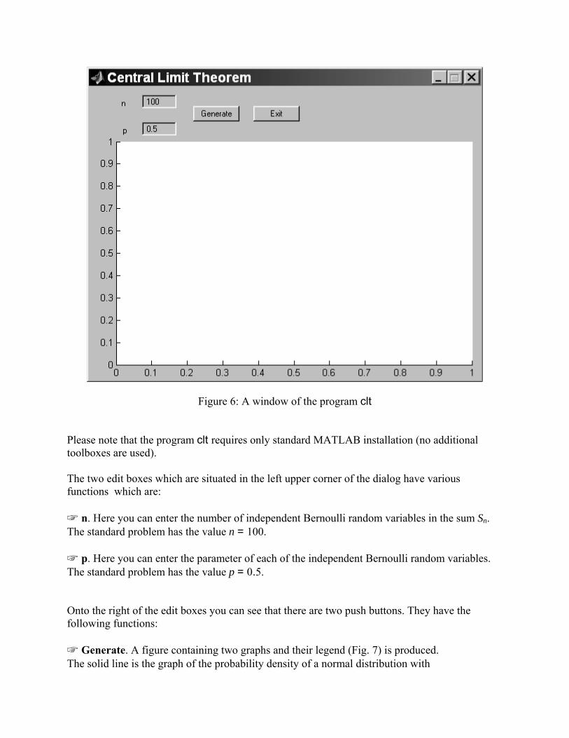
Figure 6: A window of the program clt Please note that the program clt requires only standard MATLAB installation (no additional toolboxes are used). The two edit boxes which are situated in the left upper corner of the dialog have various functions which are: ☞ n. Here you can enter the number of independent Bernoulli random variables in the sum Sn. The standard problem has the value n = 100. ☞ p. Here you can enter the parameter of each of the independent Bernoulli random variables. The standard problem has the value p = 0.5. Onto the right of the edit boxes you can see that there are two push buttons. They have the following functions: ☞ Generate. A figure containing two graphs and their legend (Fig. 7) is produced. The solid line is the graph of the probability density of a normal distribution with
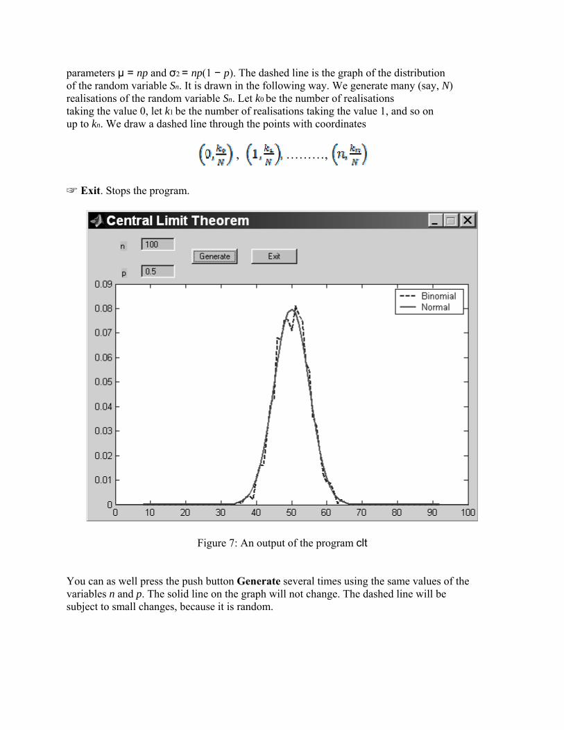
parameters μ = np and σ2 = np(1 − p). The dashed line is the graph of the distribution of the random variable Sn. It is drawn in the following way. We generate many (say, N) realisations of the random variable Sn. Let k0 be the number of realisations taking the value 0, let k1 be the number of realisations taking the value 1, and so on up to kn. We draw a dashed line through the points with coordinates
, ………,
☞ Exit. Stops the program.
Figure 7: An output of the program clt
You can as well press the push button Generate several times using the same values of the variables n and p. The solid line on the graph will not change. The dashed line will be subject to small changes, because it is random.
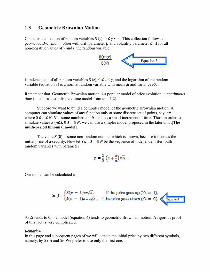
1.3 Geometric Brownian Motion Consider a collection of random variables S (y), 0 ≤ y < ∞. This collection follows a geometric Brownian motion with drift parameter μ and volatility parameter σ, if for all non-negative values of y and t, the random variable
is independent of all random variables S (z), 0 ≤ z < y, and the logarithm of the random variable (equation 3) is a normal random variable with mean μt and variance tσ2 . Remember that ,Geometric Brownian motion is a popular model of price evolution in continuous time (in contrast to a discrete time model from unit 1.2).
Suppose we want to build a computer model of the geometric Brownian motion. A computer can simulate values of any function only at some discrete set of points, say, n∆, where 0 ≤ n ≤ N, N is some number and ∆ denotes a small increment of time. Thus, in order to simulate values S (n∆), 0 ≤ n ≤ N, we can use a simpler model proposed in the later unit ,[The multi-period binomial model].
The value S (0) is some non-random number which is known, because it denotes the initial price of a security. Now let Yn, 1 ≤ n ≤ N be the sequence of independent Bernoulli random variables with parameter
Our model can be calculated as,
S(n) =
As ∆ tends to 0, the model (equation 4) tends to geometric Brownian motion. A rigorous proof of this fact is very complicated.
Remark 4. In this page and subsequent pages of we will denote the initial price by two different symbols, namely, by S (0) and S0. We prefer to use only the first one.
Equation 3
Equation4
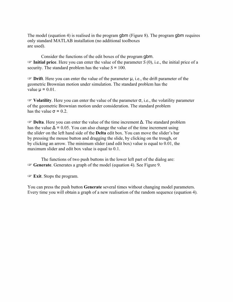
The model (equation 4) is realised in the program gbm (Figure 8). The program gbm requires only standard MATLAB installation (no additional toolboxes are used).
Consider the functions of the edit boxes of the program gbm. ☞ Initial price. Here you can enter the value of the parameter S (0), i.e., the initial price of a security. The standard problem has the value S = 100. ☞ Drift. Here you can enter the value of the parameter μ, i.e., the drift parameter of the geometric Brownian motion under simulation. The standard problem has the value μ = 0.01. ☞ Volatility. Here you can enter the value of the parameter σ, i.e., the volatility parameter of the geometric Brownian motion under consideration. The standard problem has the value σ = 0.2. ☞ Delta. Here you can enter the value of the time increment ∆. The standard problem has the value ∆ = 0.05. You can also change the value of the time increment using the slider on the left hand side of the Delta edit box. You can move the slider’s bar by pressing the mouse button and dragging the slide, by clicking on the trough, or by clicking an arrow. The minimum slider (and edit box) value is equal to 0.01, the maximum slider and edit box value is equal to 0.1.
The functions of two push buttons in the lower left part of the dialog are: ☞ Generate. Generates a graph of the model (equation 4). See Figure 9. ☞ Exit. Stops the program. You can press the push button Generate several times without changing model parameters. Every time you will obtain a graph of a new realisation of the random sequence (equation 4).
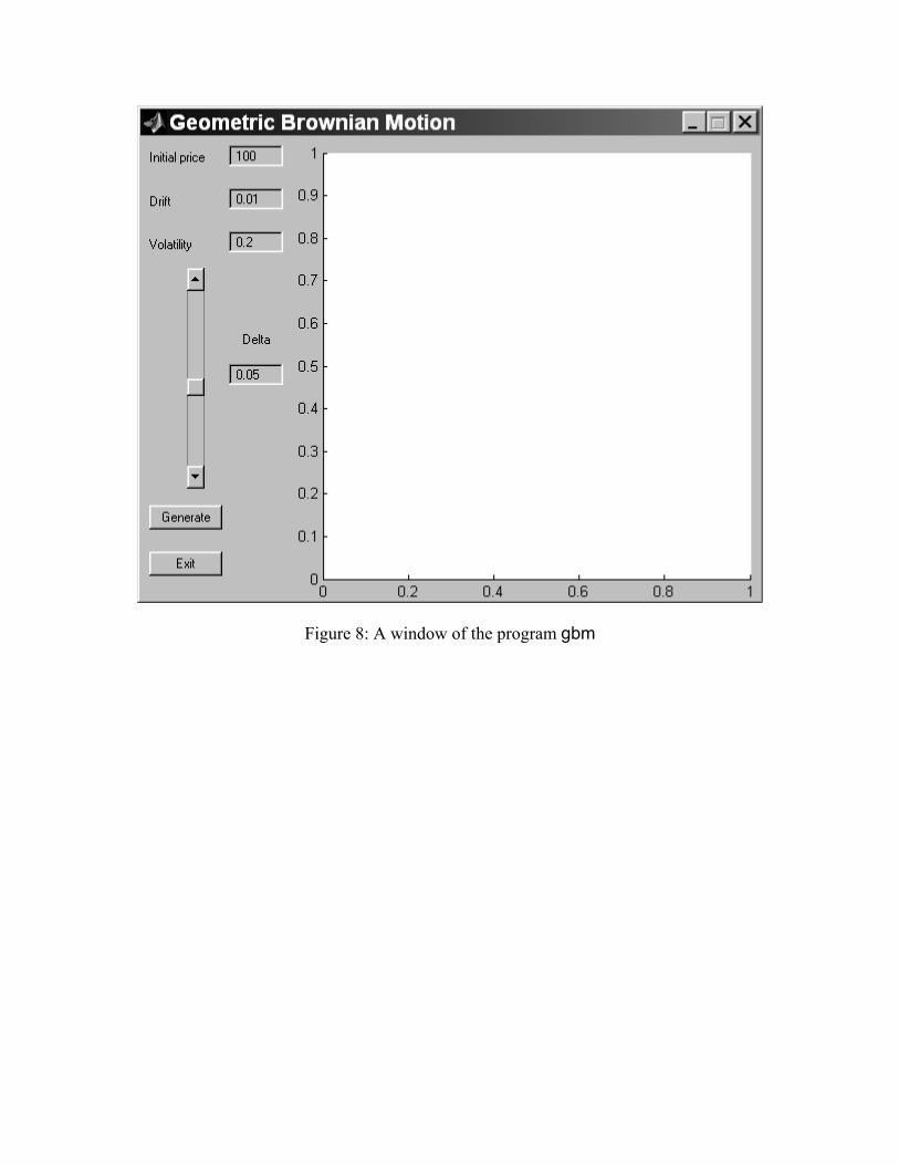
Figure 8: A window of the program gbm
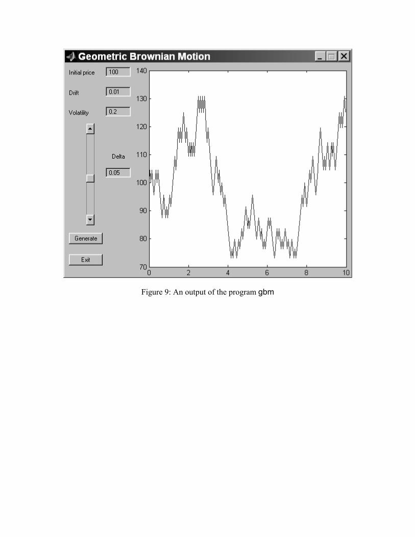
Figure 9: An output of the program gbm
UNIT TWO 2.0 Elementary financial calculations The elementary financial calculations are common methods used in solving elementary financial problems.
2.1 Interest rates Recall that the principal is an amount of borrowed money which must be repaid along with some interest. Denote the principal by P. An nominal annual interest rate or simple interest r means that the amount to be repaid one year later is P(1 + r).
Different financial institutions use various compound interests. For example, the interest can be compounded semi-annually. It means, that after six months you owe P(1+r/2), and after one year you pay P(1 + r/2)2.Similarly, if the loan is compounded at n equal intervals in the year, then the amount owed at the end of the year is P(1 + r/n)n.
In order to compare different compound interests we use the effective annual interest rate. The payment made on a one-year loan with compound interest is the same as if the loan called for simple interest at the effective annual interest rate. If we denote the effective annual interest rate by reff, then this definition can be expressed mathematically as
reff = (1 + r/n)n – 1 A continuous compounding is naturally referred as the limit of this process as n growth larger and larger. In this case the amount owed at the end of the year is
= Per.
Similarly, if the principal P is borrowed for t years at a nominal interest rate of r per year compounded continuously, then the amount owed at time t is
= Perr.
The program interest_rate (Figure 10) calculates different compound interests and shows the corresponding graphs.
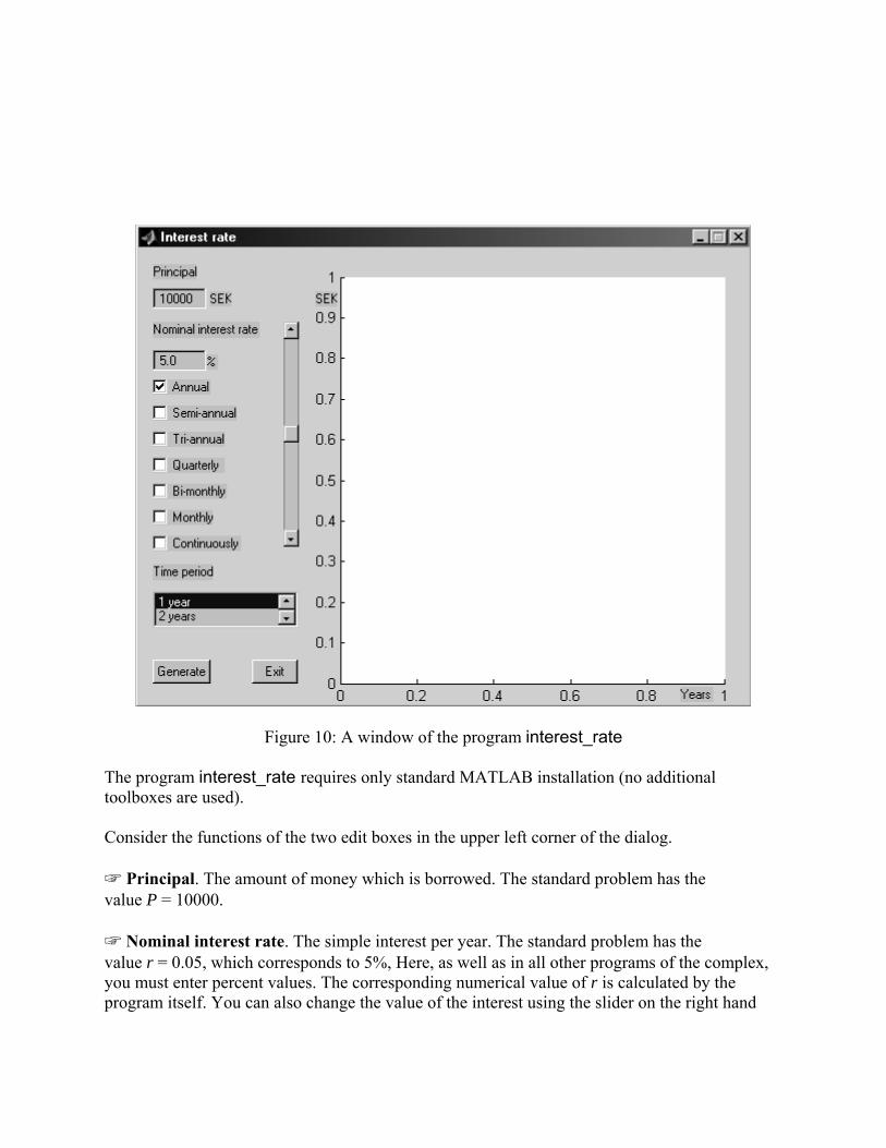
Figure 10: A window of the program interest_rate The program interest_rate requires only standard MATLAB installation (no additional toolboxes are used). Consider the functions of the two edit boxes in the upper left corner of the dialog. ☞ Principal. The amount of money which is borrowed. The standard problem has the value P = 10000. ☞ Nominal interest rate. The simple interest per year. The standard problem has the value r = 0.05, which corresponds to 5%, Here, as well as in all other programs of the complex, you must enter percent values. The corresponding numerical value of r is calculated by the program itself. You can also change the value of the interest using the slider on the right hand

side of the Nominal interest rate edit box. The minimum slider (and edit box) value is equal to 0%, the maximum slider and edit box value is equal to 10%.
Seven checkboxes are situated below the edit boxes. The checked state of any box means that the corresponding compound interest will be calculated. Consider these checkboxes in more details. ☞ Annual. Corresponds to the value n = 1, i.e. the simple interest. The interest is compound annually. The standard problem calculates this kind of interest. ☞ Semi-annual. Corresponds to the value n = 2. The interest is compound every 6 months. The standard problem does not calculate this kind of interest. ☞ Tri-annual. Corresponds to the value n = 3. The interest is compound every 4 months. The standard problem does not calculate this kind of interest. ☞ Quarterly. Corresponds to the value n = 4. The interest is compound every 3 months. The standard problem does not calculate this kind of interest. ☞ Bi-monthly. Corresponds to the value n = 6. The interest is compound every 2 months. The standard problem does not calculate this kind of interest. ☞ Monthly. Corresponds to the value n = 12. The interest is compound every month. The standard problem does not calculate this kind of interest. ☞ Continuously. Corresponds to the limit, when n growths larger and larger. The interest is compound continuously. The standard problem does not calculate this kind of interest. A list box under the checkboxes contains five elements. It determines the borrowing time (in years) and can take values 1, 2, 3, 4 or 5 years. You can choose any of these terms from the list. The standard problem has value t = 5 years. The functions of the two push buttons in the lower left part of the dialog are: ☞ Generate. Generates a graph of the repay. See Fig. 11. If no checkboxes are checked, an error message is generated instead. ☞ Exit. Stops the program. The graph (Figure 11) shows the time dependence of different compound schemes chosen by the user. A legend explains which line corresponds to which scheme, and shows the corresponding effective interest rate.
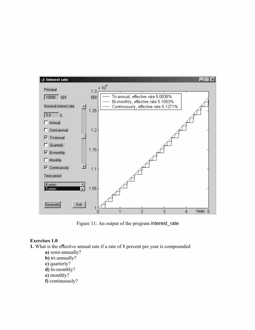
Figure 11: An output of the program interest_rate Exercises 1.0 1. What is the effective annual rate if a rate of 8 percent per year is compounded
a) semi-annually? b) tri-annually? c) quarterly? d) bi-monthly? e) monthly? f) continuously?
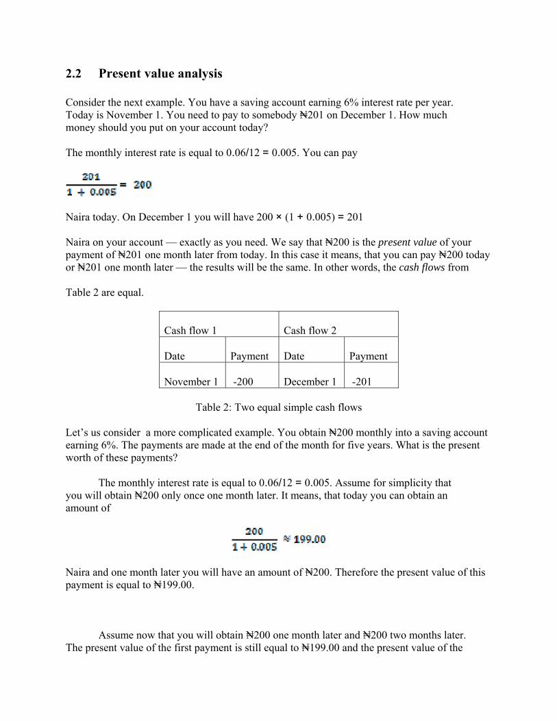
2.2 Present value analysis Consider the next example. You have a saving account earning 6% interest rate per year. Today is November 1. You need to pay to somebody ₦201 on December 1. How much money should you put on your account today? The monthly interest rate is equal to 0.06/12 = 0.005. You can pay
Naira today. On December 1 you will have 200 × (1 + 0.005) = 201 Naira on your account — exactly as you need. We say that ₦200 is the present value of your payment of ₦201 one month later from today. In this case it means, that you can pay ₦200 today or ₦201 one month later — the results will be the same. In other words, the cash flows from Table 2 are equal.
Cash flow 1
Cash flow 2
Date
Payment
Date
Payment
November 1
-200
December 1
-201
Table 2: Two equal simple cash flows
Let’s us consider a more complicated example. You obtain ₦200 monthly into a saving account earning 6%. The payments are made at the end of the month for five years. What is the present worth of these payments?
The monthly interest rate is equal to 0.06/12 = 0.005. Assume for simplicity that you will obtain ₦200 only once one month later. It means, that today you can obtain an amount of
Naira and one month later you will have an amount of ₦200. Therefore the present value of this payment is equal to ₦199.00.
Assume now that you will obtain ₦200 one month later and ₦200 two months later. The present value of the first payment is still equal to ₦199.00 and the present value of the
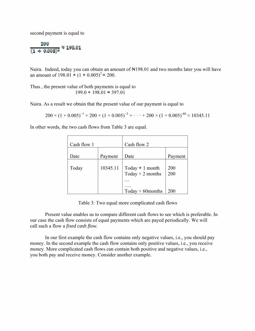
second payment is equal to
Naira. Indeed, today you can obtain an amount of ₦198.01 and two months later you will have an amount of 198.01 × (1 + 0.005)2
= 200. Thus , the present value of both payments is equal to
199.0 + 198.01 ≈ 397.01 Naira. As a result we obtain that the present value of our payment is equal to
200 × (1 + 0.005)−1 + 200 × (1 + 0.005)−2 + · · · + 200 × (1 + 0.005)-60 ≈ 10345.11
In other words, the two cash flows from Table 3 are equal.
Cash flow 1
Cash flow 2
Date
Payment
Date
Payment
Today
10345.11
Today + 1 month Today + 2 months … …. Today + 60months
200 200 200
Table 3: Two equal more complicated cash flows
Present value enables us to compare different cash flows to see which is preferable. In
our case the cash flow consists of equal payments which are payed periodically. We will call such a flow a fixed cash flow.
In our first example the cash flow contains only negative values, i.e., you should pay money. In the second example the cash flow contains only positive values, i.e., you receive money. More complicated cash flows can contain both positive and negative values, i.e., you both pay and receive money. Consider another example.
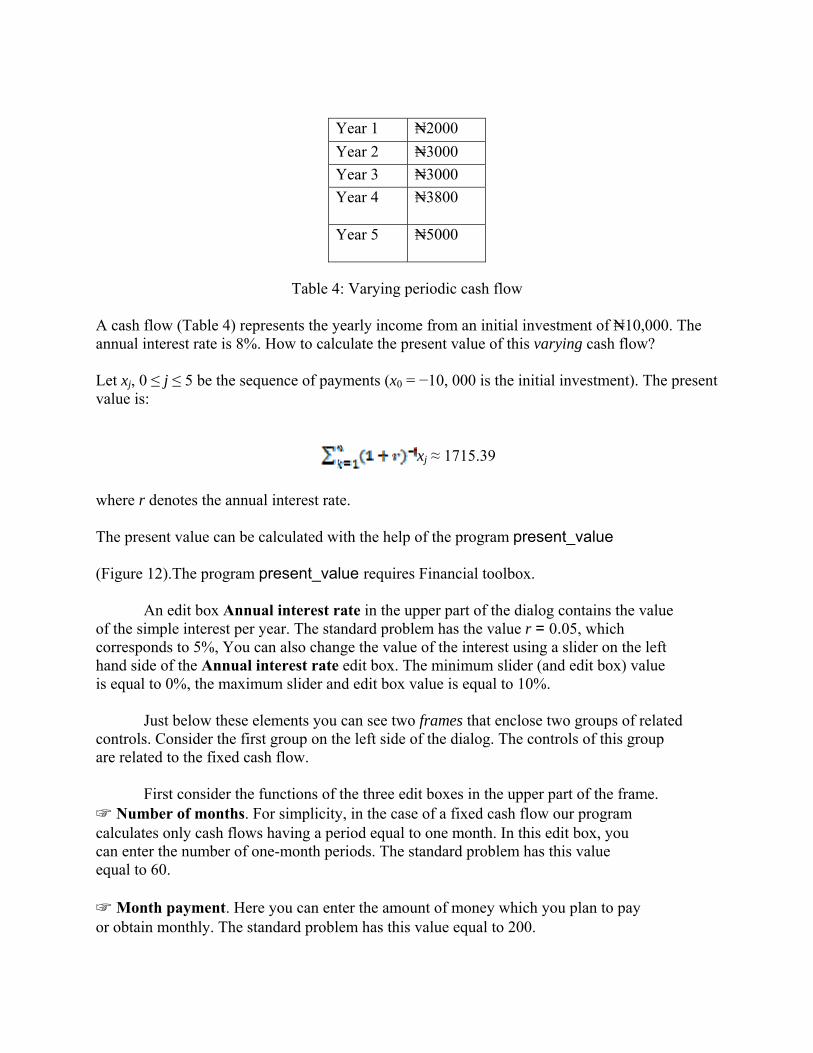
Table 4: Varying periodic cash flow
A cash flow (Table 4) represents the yearly income from an initial investment of ₦10,000. The annual interest rate is 8%. How to calculate the present value of this varying cash flow? Let xj, 0 ≤ j ≤ 5 be the sequence of payments (x0 = −10, 000 is the initial investment). The present value is:
xj ≈ 1715.39
where r denotes the annual interest rate. The present value can be calculated with the help of the program present_value (Figure 12).The program present_value requires Financial toolbox.
An edit box Annual interest rate in the upper part of the dialog contains the value of the simple interest per year. The standard problem has the value r = 0.05, which corresponds to 5%, You can also change the value of the interest using a slider on the left hand side of the Annual interest rate edit box. The minimum slider (and edit box) value is equal to 0%, the maximum slider and edit box value is equal to 10%.
Just below these elements you can see two frames that enclose two groups of related controls. Consider the first group on the left side of the dialog. The controls of this group are related to the fixed cash flow.
First consider the functions of the three edit boxes in the upper part of the frame. ☞ Number of months. For simplicity, in the case of a fixed cash flow our program calculates only cash flows having a period equal to one month. In this edit box, you can enter the number of one-month periods. The standard problem has this value equal to 60. ☞ Month payment. Here you can enter the amount of money which you plan to pay or obtain monthly. The standard problem has this value equal to 200.
Year 1 ₦2000
Year 2 ₦3000
Year 3 ₦3000
Year 4 ₦3800
Year 5 ₦5000
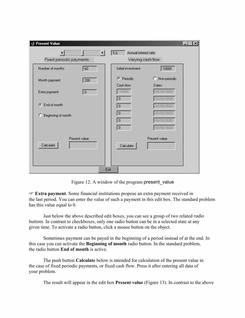
Figure 12: A window of the program present_value
☞ Extra payment. Some financial institutions propose an extra payment received in the last period. You can enter the value of such a payment in this edit box. The standard problem has this value equal to 0.
Just below the above described edit boxes, you can see a group of two related radio buttons. In contrast to checkboxes, only one radio button can be in a selected state at any given time. To activate a radio button, click a mouse button on the object.
Sometimes payment can be payed in the beginning of a period instead of at the end. In this case you can activate the Beginning of month radio button. In the standard problem, the radio button End of month is active.
The push button Calculate below is intended for calculation of the present value in the case of fixed periodic payments, or fixed cash flow. Press it after entering all data of your problem.
The result will appear in the edit box Present value (Figure 13). In contrast to the above
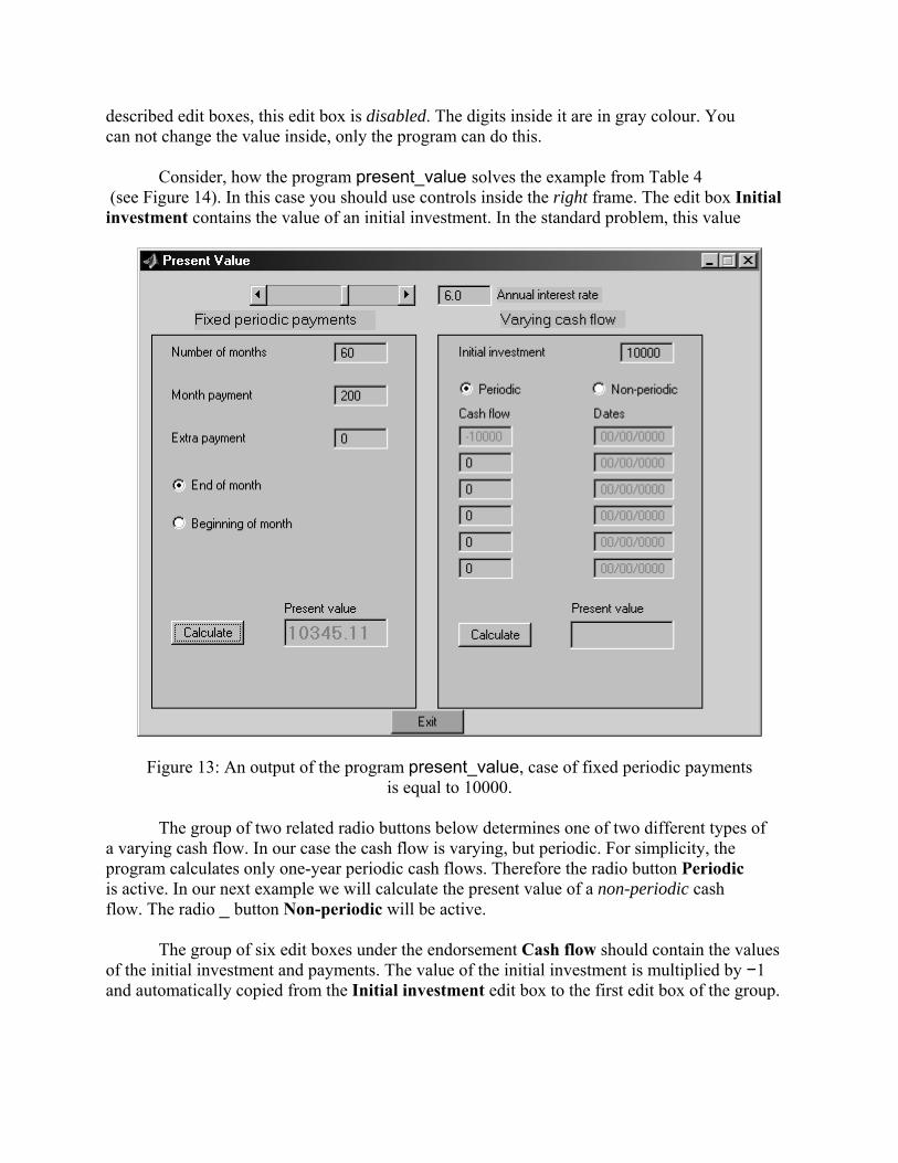
described edit boxes, this edit box is disabled. The digits inside it are in gray colour. You can not change the value inside, only the program can do this.
Consider, how the program present_value solves the example from Table 4 (see Figure 14). In this case you should use controls inside the right frame. The edit box Initial investment contains the value of an initial investment. In the standard problem, this value
Figure 13: An output of the program present_value, case of fixed periodic payments is equal to 10000.
The group of two related radio buttons below determines one of two different types of
a varying cash flow. In our case the cash flow is varying, but periodic. For simplicity, the program calculates only one-year periodic cash flows. Therefore the radio button Periodic is active. In our next example we will calculate the present value of a non-periodic cash flow. The radio _ button Non-periodic will be active.
The group of six edit boxes under the endorsement Cash flow should contain the values of the initial investment and payments. The value of the initial investment is multiplied by −1 and automatically copied from the Initial investment edit box to the first edit box of the group.
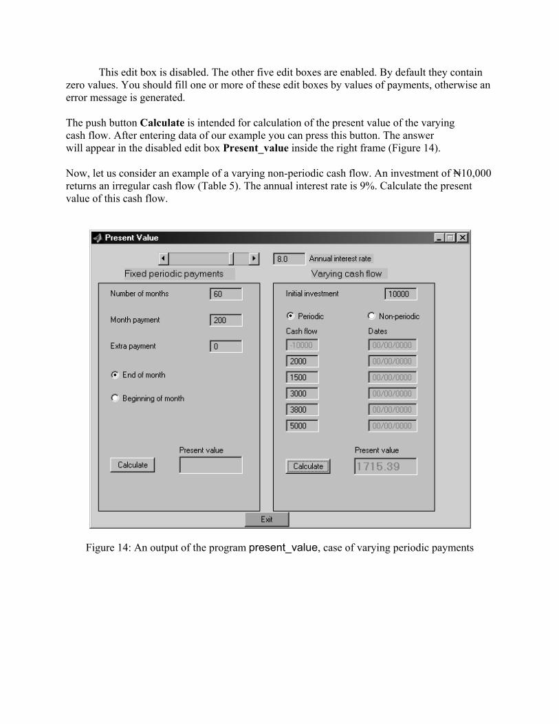
This edit box is disabled. The other five edit boxes are enabled. By default they contain zero values. You should fill one or more of these edit boxes by values of payments, otherwise an error message is generated. The push button Calculate is intended for calculation of the present value of the varying cash flow. After entering data of our example you can press this button. The answer will appear in the disabled edit box Present_value inside the right frame (Figure 14). Now, let us consider an example of a varying non-periodic cash flow. An investment of ₦10,000 returns an irregular cash flow (Table 5). The annual interest rate is 9%. Calculate the present value of this cash flow.
Figure 14: An output of the program present_value, case of varying periodic payments
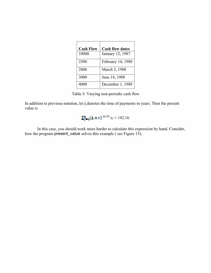
Table 5: Varying non-periodic cash flow
In addition to previous notation, let tj denotes the time of payments in years. Then the present value is
-(tj-t0) xj ≈ 142.16.
In this case, you should work more harder to calculate this expression by hand. Consider,
how the program present_value solves this example ( see Figure 15).
Cash Flow
Cash flow dates
10000 January 12, 1987
2500 February 14, 1988
2000 March 3, 1988
3000 June 14, 1988
4000 December 1, 1988
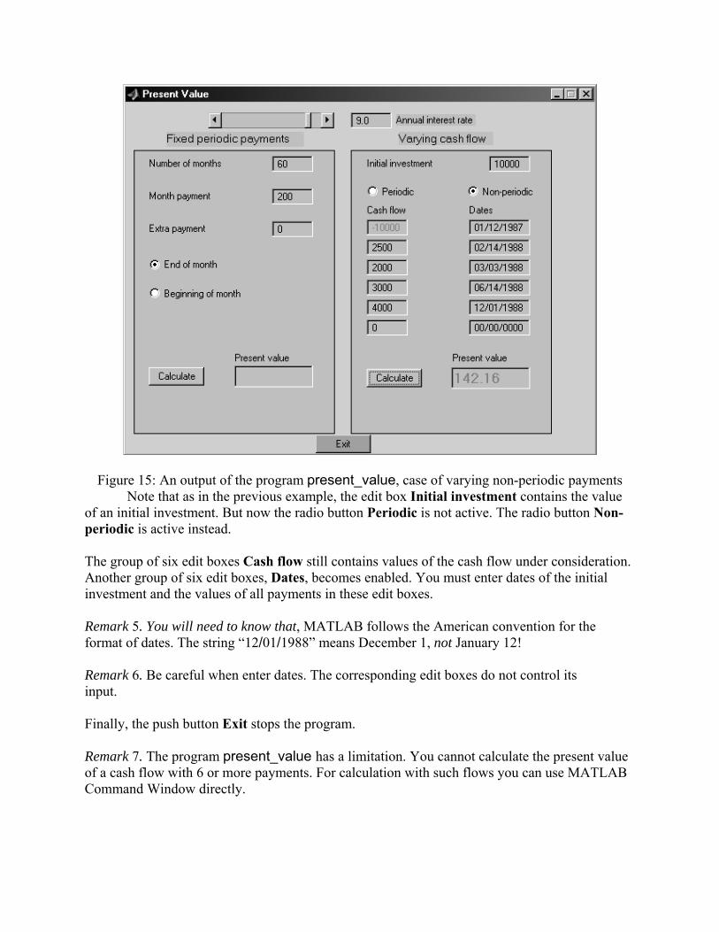
Figure 15: An output of the program present_value, case of varying non-periodic payments Note that as in the previous example, the edit box Initial investment contains the value
of an initial investment. But now the radio button Periodic is not active. The radio button Non-periodic is active instead. The group of six edit boxes Cash flow still contains values of the cash flow under consideration. Another group of six edit boxes, Dates, becomes enabled. You must enter dates of the initial investment and the values of all payments in these edit boxes. Remark 5. You will need to know that, MATLAB follows the American convention for the format of dates. The string “12/01/1988” means December 1, not January 12! Remark 6. Be careful when enter dates. The corresponding edit boxes do not control its input. Finally, the push button Exit stops the program. Remark 7. The program present_value has a limitation. You cannot calculate the present value of a cash flow with 6 or more payments. For calculation with such flows you can use MATLAB Command Window directly.
2.2.1 Problems 1. ₦150 is paid monthly into a saving account earning 4%. The payments are made at the end of the month for ten years. What is the present value of these payments? 2. ₦250 is paid monthly into a saving account earning 5%. The payments are made at the beginning of the month for seven years. What is the present worth of these payments? UNIT THREE 3.0 Rate of return
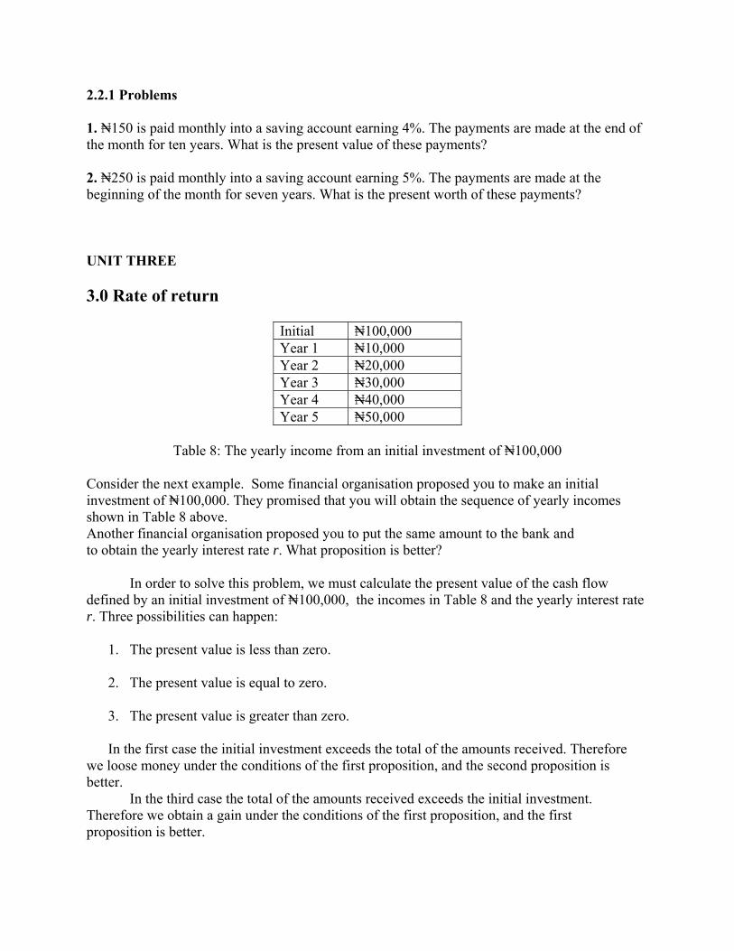
Initial ₦100,000 Year 1 ₦10,000 Year 2 ₦20,000 Year 3 ₦30,000 Year 4 ₦40,000 Year 5 ₦50,000
Table 8: The yearly income from an initial investment of ₦100,000
Consider the next example. Some financial organisation proposed you to make an initial investment of ₦100,000. They promised that you will obtain the sequence of yearly incomes shown in Table 8 above. Another financial organisation proposed you to put the same amount to the bank and to obtain the yearly interest rate r. What proposition is better?
In order to solve this problem, we must calculate the present value of the cash flow defined by an initial investment of ₦100,000, the incomes in Table 8 and the yearly interest rate r. Three possibilities can happen:
1. The present value is less than zero.
2. The present value is equal to zero.
3. The present value is greater than zero.
In the first case the initial investment exceeds the total of the amounts received. Therefore
we loose money under the conditions of the first proposition, and the second proposition is better.
In the third case the total of the amounts received exceeds the initial investment. Therefore we obtain a gain under the conditions of the first proposition, and the first proposition is better.
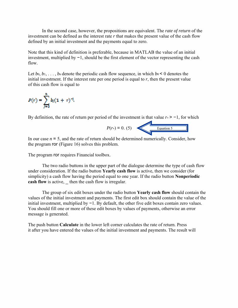
In the second case, however, the propositions are equivalent. The rate of return of the investment can be defined as the interest rate r that makes the present value of the cash flow defined by an initial investment and the payments equal to zero.
Note that this kind of definition is preferable, because in MATLAB the value of an initial investment, multiplied by −1, should be the first element of the vector representing the cash flow. Let b0, b1, . . . , bn denote the periodic cash flow sequence, in which b0 < 0 denotes the initial investment. If the interest rate per one period is equal to r, then the present value of this cash flow is equal to
By definition, the rate of return per period of the investment is that value r∗ > −1, for which
P(r∗) = 0. (5)
In our case n = 5, and the rate of return should be determined numerically. Consider, how the program ror (Figure 16) solves this problem. The program ror requires Financial toolbox.
The two radio buttons in the upper part of the dialogue determine the type of cash flow under consideration. If the radio button Yearly cash flow is active, then we consider (for simplicity) a cash flow having the period equal to one year. If the radio button Nonperiodic cash flow is active, _ then the cash flow is irregular.
The group of six edit boxes under the radio button Yearly cash flow should contain the values of the initial investment and payments. The first edit box should contain the value of the initial investment, multiplied by −1. By default, the other five edit boxes contain zero values. You should fill one or more of these edit boxes by values of payments, otherwise an error message is generated. The push button Calculate in the lower left corner calculates the rate of return. Press it after you have entered the values of the initial investment and payments. The result will
Equation 5
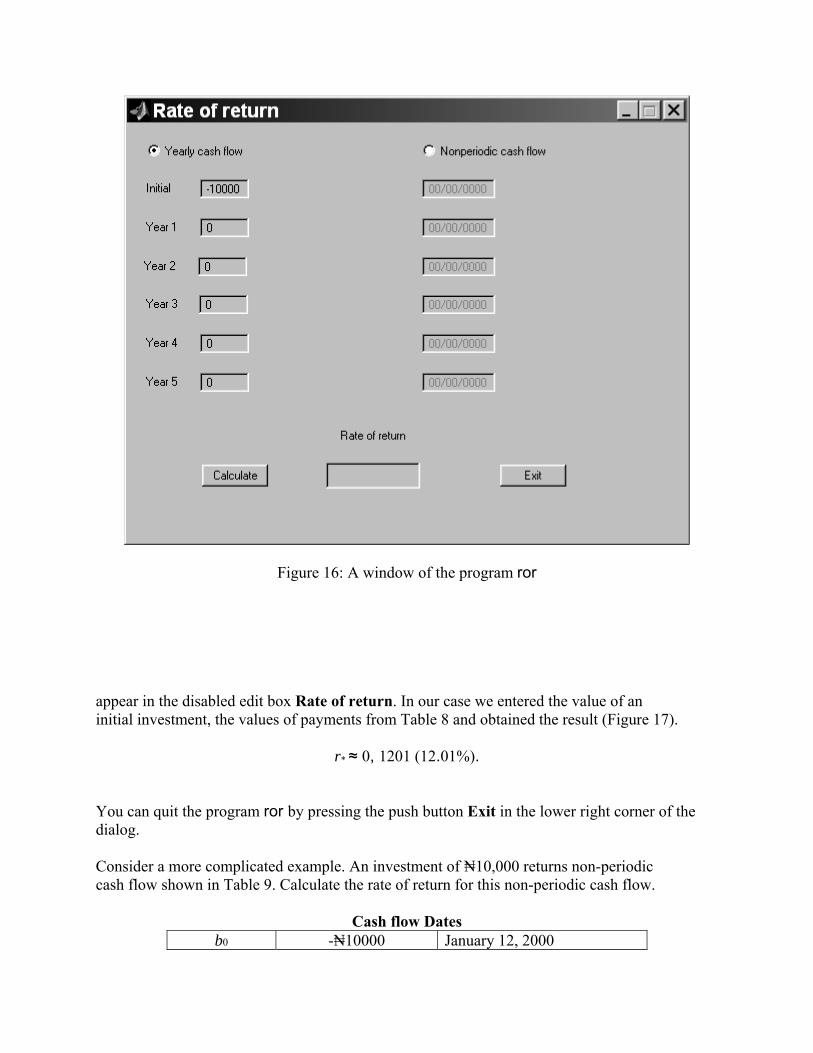
Figure 16: A window of the program ror
appear in the disabled edit box Rate of return. In our case we entered the value of an initial investment, the values of payments from Table 8 and obtained the result (Figure 17).
r∗ ≈ 0, 1201 (12.01%).
You can quit the program ror by pressing the push button Exit in the lower right corner of the dialog. Consider a more complicated example. An investment of ₦10,000 returns non-periodic cash flow shown in Table 9. Calculate the rate of return for this non-periodic cash flow.
Cash flow Dates b0 -₦10000 January 12, 2000
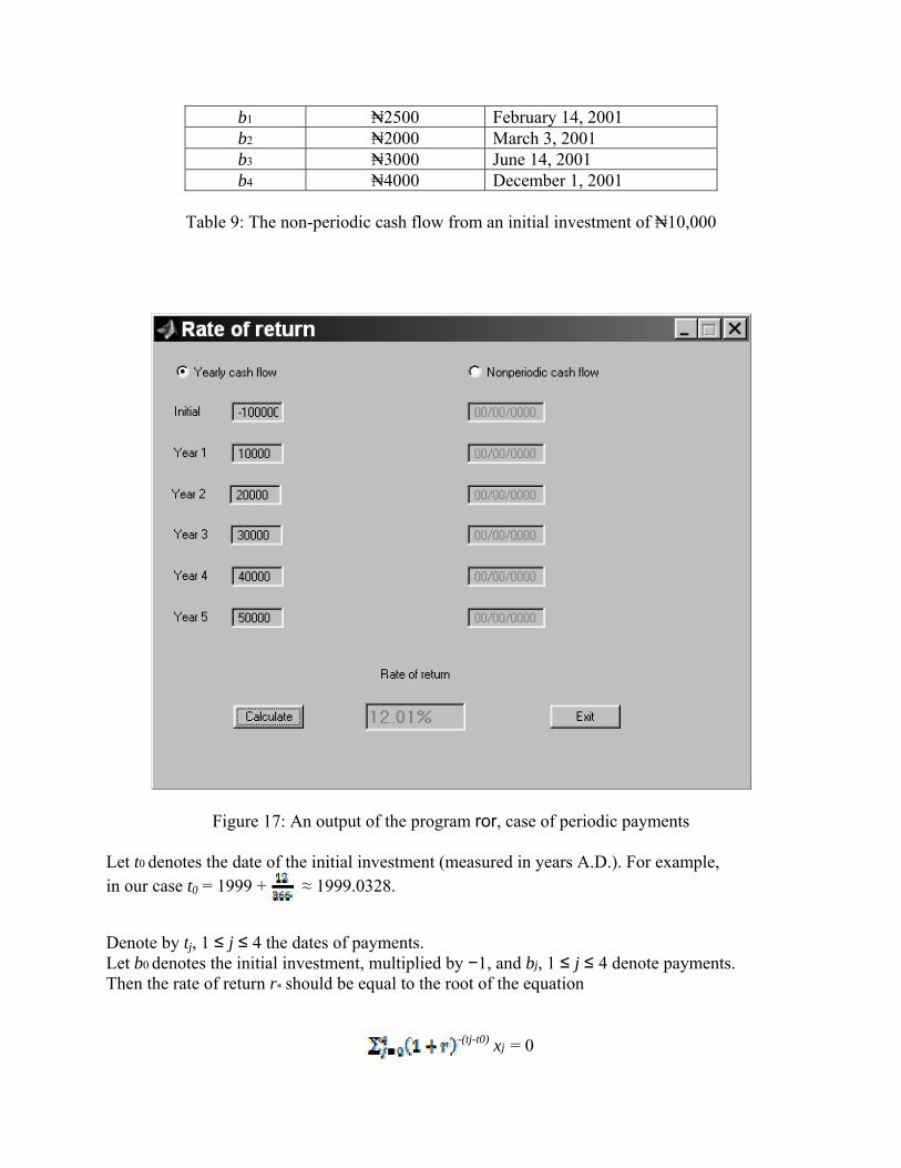
b1 ₦2500 February 14, 2001 b2 ₦2000 March 3, 2001 b3 ₦3000 June 14, 2001 b4 ₦4000 December 1, 2001
Table 9: The non-periodic cash flow from an initial investment of ₦10,000
Figure 17: An output of the program ror, case of periodic payments
Let t0 denotes the date of the initial investment (measured in years A.D.). For example, in our case t0 = 1999 + ≈ 1999.0328.
Denote by tj, 1 ≤ j ≤ 4 the dates of payments. Let b0 denotes the initial investment, multiplied by −1, and bj, 1 ≤ j ≤ 4 denote payments. Then the rate of return r∗ should be equal to the root of the equation
-(tj-t0) xj = 0
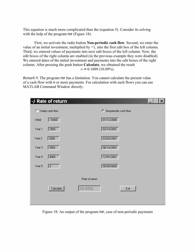
This equation is much more complicated than the (equation 5). Consider its solving with the help of the program ror (Figure 18).
First, we activate the radio button Non-periodic cash flow. Second, we enter the value of an initial investment, multiplied by −1, into the first edit box of the left column. Third, we entered values of payments into next edit boxes of the left column. Now, the edit boxes of the right column are enabled (in the previous example they were disabled). We entered dates of the initial investment and payments into the edit boxes of the right column. After pressing the push button Calculate, we obtained the result
r∗ ≈ 0.1009 (10.09%).
Remark 9. The program ror has a limitation. You cannot calculate the present value of a cash flow with 6 or more payments. For calculation with such flows you can use MATLAB Command Window directly.
Figure 18: An output of the program ror, case of non-periodic payments
Exercises 1. The initial investment of ₦4,400 returns the yearly cash flow shown in Table 6.You can both borrow and save money at the yearly interest rate of 6%. Is this a worthwhile investment for you? 3.1 Pricing via arbitrage Recall that an option gives the buyer the right, but not the obligation, to buy or sell a security under specified terms. An option that gives the right to buy is called a call option. An option that gives the right to sell is called a put option. Consider the example of a call option.
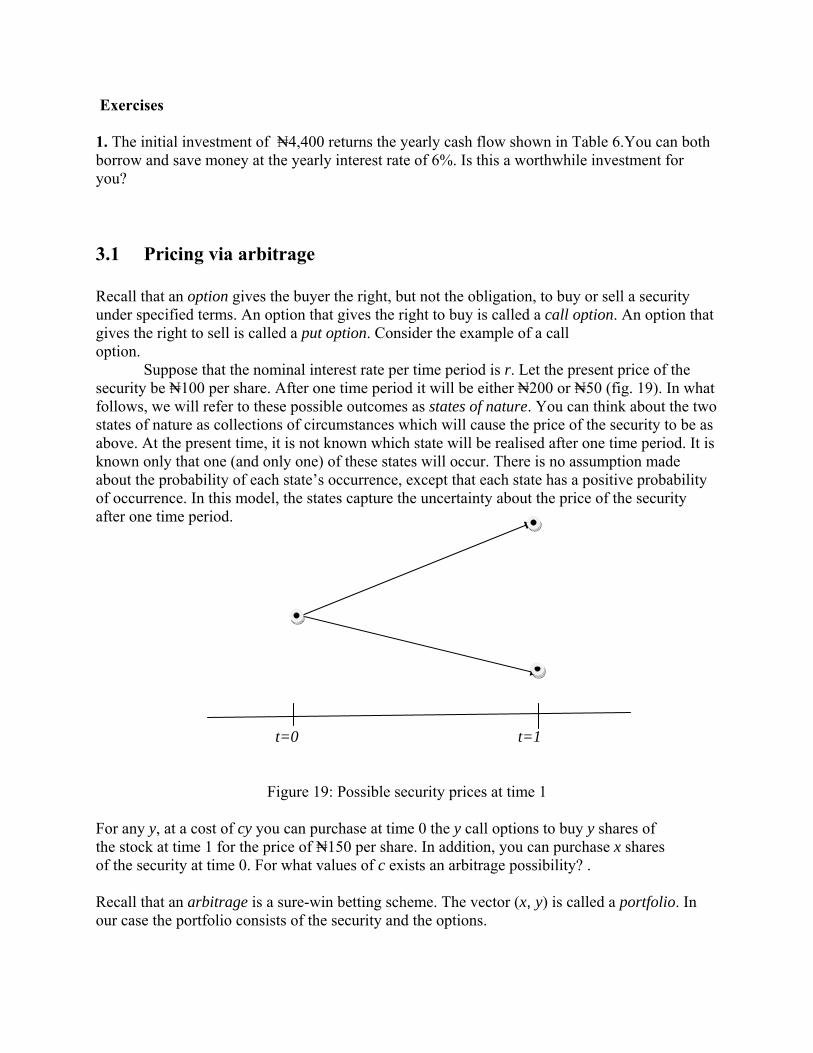
Suppose that the nominal interest rate per time period is r. Let the present price of the security be ₦100 per share. After one time period it will be either ₦200 or ₦50 (fig. 19). In what follows, we will refer to these possible outcomes as states of nature. You can think about the two states of nature as collections of circumstances which will cause the price of the security to be as above. At the present time, it is not known which state will be realised after one time period. It is known only that one (and only one) of these states will occur. There is no assumption made about the probability of each state’s occurrence, except that each state has a positive probability of occurrence. In this model, the states capture the uncertainty about the price of the security after one time period. t=0 t=1
Figure 19: Possible security prices at time 1
For any y, at a cost of cy you can purchase at time 0 the y call options to buy y shares of the stock at time 1 for the price of ₦150 per share. In addition, you can purchase x shares of the security at time 0. For what values of c exists an arbitrage possibility? . Recall that an arbitrage is a sure-win betting scheme. The vector (x, y) is called a portfolio. In our case the portfolio consists of the security and the options.
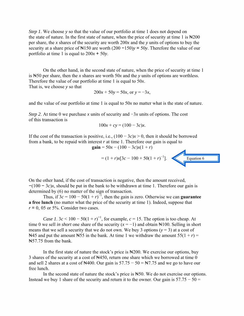
Step 1. We choose y so that the value of our portfolio at time 1 does not depend on the state of nature. In the first state of nature, when the price of security at time 1 is ₦200 per share, the x shares of the security are worth 200x and the y units of options to buy the security at a share price of ₦150 are worth (200 −150)y = 50y. Therefore the value of our portfolio at time 1 is equal to 200x + 50y.
On the other hand, in the second state of nature, when the price of security at time 1 is ₦50 per share, then the x shares are worth 50x and the y units of options are worthless. Therefore the value of our portfolio at time 1 is equal to 50x. That is, we choose y so that
200x + 50y = 50x, or y = −3x,
and the value of our portfolio at time 1 is equal to 50x no matter what is the state of nature. Step 2. At time 0 we purchase x units of security and −3x units of options. The cost of this transaction is
100x + cy = (100 − 3c)x.
If the cost of the transaction is positive, i.e., (100 − 3c)x > 0, then it should be borrowed from a bank, to be repaid with interest r at time 1. Therefore our gain is equal to
gain = 50x − (100 − 3c)x(1 + r)
= (1 + r)x[3c − 100 + 50(1 + r)−1]. On the other hand, if the cost of transaction is negative, then the amount received, −(100 − 3c)x, should be put in the bank to be withdrawn at time 1. Therefore our gain is determined by (6) no matter of the sign of transaction.
Thus, if 3c = 100 − 50(1 + r)−1, then the gain is zero. Otherwise we can guarantee a free lunch (no matter what the price of the security at time 1). Indeed, suppose that r = 0, 05 or 5%. Consider two cases.
Case 1. 3c < 100 − 50(1 + r)−1, for example, c = 15. The option is too cheap. At time 0 we sell in short one share of the security (x = −1) and obtain ₦100. Selling in short means that we sell a security that we do not own. We buy 3 options (y = 3) at a cost of ₦45 and put the amount ₦55 in the bank. At time 1 we withdraw the amount 55(1 + r) = ₦57.75 from the bank.
In the first state of nature the stock’s price is ₦200. We exercise our options, buy 3 shares of the security at a cost of ₦450, return one share which we borrowed at time 0 and sell 2 shares at a cost of ₦400. Our gain is 57.75 − 50 = ₦7.75 and we go to have our free lunch.
In the second state of nature the stock’s price is ₦50. We do not exercise our options. Instead we buy 1 share of the security and return it to the owner. Our gain is 57.75 − 50 =
Equation 6
₦7.75 and we go to have our free lunch.
Case 2. 3c > 100 − 50(1 + r)−1, for example, c = 20. The option is too expensive. At time 0 we borrow from a bank ₦40. We sell in short 3 options at a cost of ₦60 (y = −3) and buy 1 share of the security (x = 1).
In the first state of nature the stock’s price is ₦200. The options’ owner realises the options. We are obliged to buy 3 shares at a cost of ₦600 and sell them to the options’ owner at a cost of 450. Then we sell our share at a cost of ₦200. The amount earned is ₦50, but we have to return the loan 40 × (1 + 0.05) = ₦42 to the bank. Our gain is 50 − 42=₦8 and we go to have our free lunch.
In the second state of nature the stock’s price is ₦50. The options’ owner does not realise the options. We sell our share for ₦50, return the loan of ₦42 and go to have our free lunch.
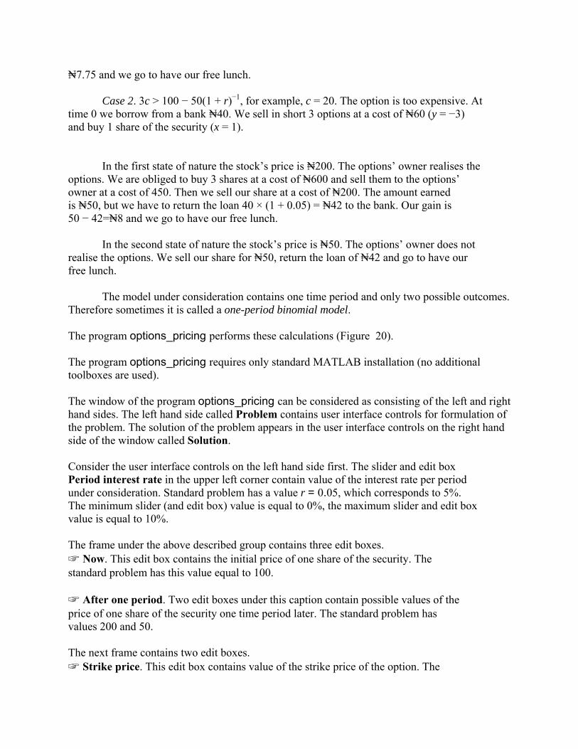
The model under consideration contains one time period and only two possible outcomes. Therefore sometimes it is called a one-period binomial model. The program options_pricing performs these calculations (Figure 20). The program options_pricing requires only standard MATLAB installation (no additional toolboxes are used). The window of the program options_pricing can be considered as consisting of the left and right hand sides. The left hand side called Problem contains user interface controls for formulation of the problem. The solution of the problem appears in the user interface controls on the right hand side of the window called Solution. Consider the user interface controls on the left hand side first. The slider and edit box Period interest rate in the upper left corner contain value of the interest rate per period under consideration. Standard problem has a value r = 0.05, which corresponds to 5%. The minimum slider (and edit box) value is equal to 0%, the maximum slider and edit box value is equal to 10%. The frame under the above described group contains three edit boxes. ☞ Now. This edit box contains the initial price of one share of the security. The standard problem has this value equal to 100. ☞ After one period. Two edit boxes under this caption contain possible values of the price of one share of the security one time period later. The standard problem has values 200 and 50. The next frame contains two edit boxes. ☞ Strike price. This edit box contains value of the strike price of the option. The
standard problem has this value equal to 150. ☞ Option cost. This edit box contains the price of the option. The standard problem has this value equal to 20.
Figure 20: The window of the program options_pricing
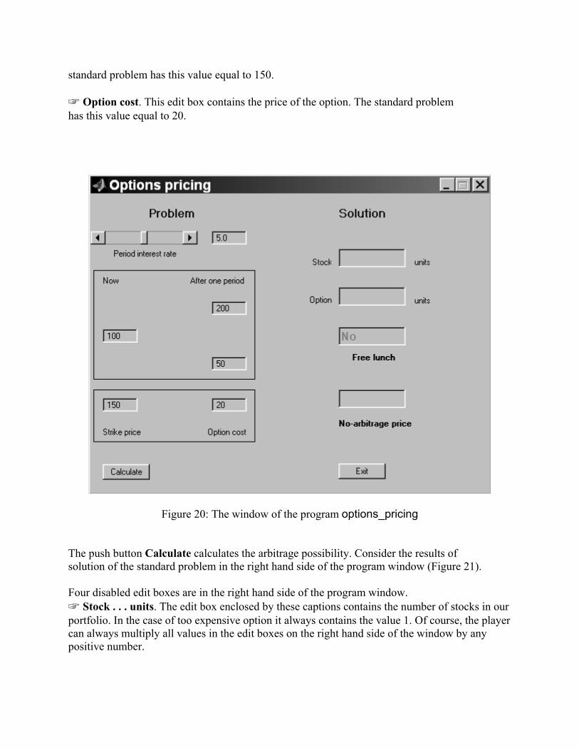
The push button Calculate calculates the arbitrage possibility. Consider the results of solution of the standard problem in the right hand side of the program window (Figure 21). Four disabled edit boxes are in the right hand side of the program window. ☞ Stock . . . units. The edit box enclosed by these captions contains the number of stocks in our portfolio. In the case of too expensive option it always contains the value 1. Of course, the player can always multiply all values in the edit boxes on the right hand side of the window by any positive number.
Figure 21: An output of the program options_pricing, case of too expensive option ☞ Option . . . units. The edit box enclosed by these captions contains the number of options in our portfolio. In our example, this value is negative. It means, that we should sell options in short. ☞ Free lunch. This edit box contains the value of our gain. ☞ No-arbitrage price. This edit box contains the value of the only option cost that does not result in an arbitrage. This price is called no-arbitrage or risk-neutral price. Pricing of an option means the calculation of its no-arbitrage or risk-neutral price. Finally, the push button Exit stops the program.
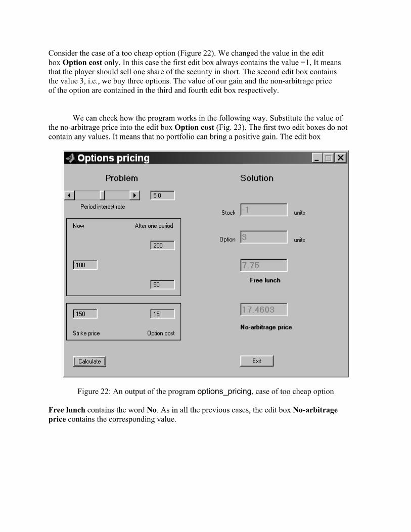
Consider the case of a too cheap option (Figure 22). We changed the value in the edit box Option cost only. In this case the first edit box always contains the value −1, It means that the player should sell one share of the security in short. The second edit box contains the value 3, i.e., we buy three options. The value of our gain and the non-arbitrage price of the option are contained in the third and fourth edit box respectively.
We can check how the program works in the following way. Substitute the value of the no-arbitrage price into the edit box Option cost (Fig. 23). The first two edit boxes do not contain any values. It means that no portfolio can bring a positive gain. The edit box
Figure 22: An output of the program options_pricing, case of too cheap option Free lunch contains the word No. As in all the previous cases, the edit box No-arbitrage price contains the corresponding value.
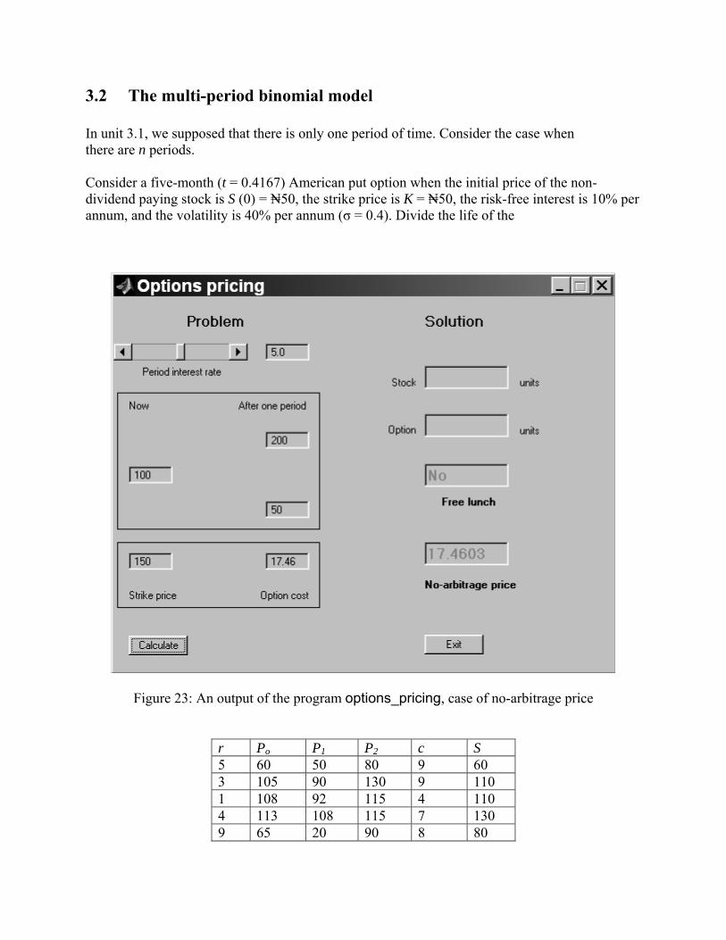
3.2 The multi-period binomial model In unit 3.1, we supposed that there is only one period of time. Consider the case when there are n periods. Consider a five-month (t = 0.4167) American put option when the initial price of the non-dividend paying stock is S (0) = ₦50, the strike price is K = ₦50, the risk-free interest is 10% per annum, and the volatility is 40% per annum (σ = 0.4). Divide the life of the
Figure 23: An output of the program options_pricing, case of no-arbitrage price
r Po P1 P2 c S 5 60 50 80 9 60 3 105 90 130 9 110 1 108 92 115 4 110 4 113 108 115 7 130 9 65 20 90 8 80
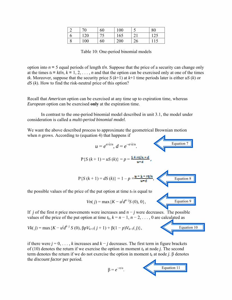
2 70 60 100 5 80 6 120 75 165 21 125 8 100 60 200 26 115
Table 10: One-period binomial models
option into n = 5 equal periods of length t/n. Suppose that the price of a security can change only at the times tk = kt/n, k = 1, 2, . . . , n and that the option can be exercised only at one of the times tk. Moreover, suppose that the security price S (k+1) at k+1 time periods later is either uS (k) or dS (k). How to find the risk-neutral price of this option? Recall that American option can be exercised at any time up to expiration time, whereas European option can be exercised only at the expiration time.
In contrast to the one-period binomial model described in unit 3.1, the model under consideration is called a multi-period binomial model. We want the above described process to approximate the geometrical Brownian motion when n grows. According to (equation 4) that happens if
u = eσ√t/n, d = e−σ√t/n.
P{S (k + 1) = uS (k)} = p =
P{S (k + 1) = dS (k)} = 1 – p = ,
the possible values of the price of the put option at time tn is equal to
Vn( j) = max{K − ujdn−jS (0), 0},
If j of the first n price movements were increases and n − j were decreases. The possible values of the price of the put option at time tk, k = n − 1, n − 2, . . . , 0 are calculated as
Vk( j) = max{K − ujdk−j S (0), βpVk+1( j + 1) + β(1 − p)Vk+1( j)},
if there were j = 0, . . . , k increases and k − j decreases. The first term in figure brackets of (10) denotes the return if we exercise the option in moment tk at node j. The second term denotes the return if we do not exercise the option in moment tk at node j. β denotes the discount factor per period.
β = e−rt/n.
Equation 7
Equation 8
Equation 9
Equation 10
Equation 11
Using these formulae, we obtain
V0(0) ≈ 4.488.
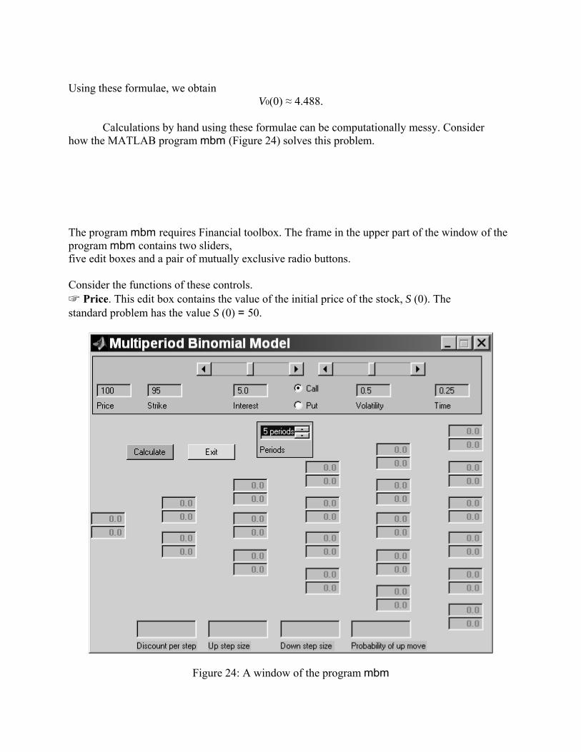
Calculations by hand using these formulae can be computationally messy. Consider how the MATLAB program mbm (Figure 24) solves this problem. The program mbm requires Financial toolbox. The frame in the upper part of the window of the program mbm contains two sliders, five edit boxes and a pair of mutually exclusive radio buttons. Consider the functions of these controls. ☞ Price. This edit box contains the value of the initial price of the stock, S (0). The standard problem has the value S (0) = 50.
Figure 24: A window of the program mbm
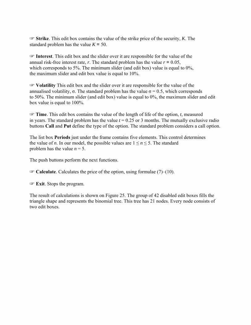
☞ Strike. This edit box contains the value of the strike price of the security, K. The standard problem has the value K = 50. ☞ Interest. This edit box and the slider over it are responsible for the value of the annual risk-free interest rate, r. The standard problem has the value r = 0.05, which corresponds to 5%. The minimum slider (and edit box) value is equal to 0%, the maximum slider and edit box value is equal to 10%. ☞ Volatility This edit box and the slider over it are responsible for the value of the annualised volatility, σ. The standard problem has the value σ = 0.5, which corresponds to 50%. The minimum slider (and edit box) value is equal to 0%, the maximum slider and edit box value is equal to 100%. ☞ Time. This edit box contains the value of the length of life of the option, t, measured in years. The standard problem has the value t = 0.25 or 3 months. The mutually exclusive radio buttons Call and Put define the type of the option. The standard problem considers a call option. The list box Periods just under the frame contains five elements. This control determines the value of n. In our model, the possible values are 1 ≤ n ≤ 5. The standard problem has the value n = 5. The push buttons perform the next functions. ☞ Calculate. Calculates the price of the option, using formulae (7)–(10). ☞ Exit. Stops the program. The result of calculations is shown on Figure 25. The group of 42 disabled edit boxes fills the triangle shape and represents the binomial tree. This tree has 21 nodes. Every node consists of two edit boxes.
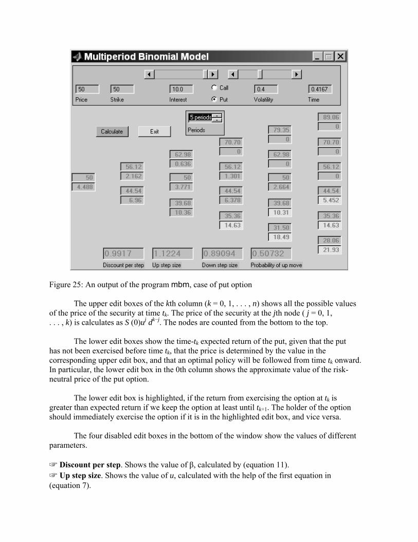
Figure 25: An output of the program mbm, case of put option
The upper edit boxes of the kth column (k = 0, 1, . . . , n) shows all the possible values of the price of the security at time tk. The price of the security at the jth node ( j = 0, 1, . . . , k) is calculates as S (0)uj dk−j. The nodes are counted from the bottom to the top.
The lower edit boxes show the time-tk expected return of the put, given that the put
has not been exercised before time tk, that the price is determined by the value in the corresponding upper edit box, and that an optimal policy will be followed from time tk onward. In particular, the lower edit box in the 0th column shows the approximate value of the risk-neutral price of the put option.
The lower edit box is highlighted, if the return from exercising the option at tk is greater than expected return if we keep the option at least until tk+1. The holder of the option should immediately exercise the option if it is in the highlighted edit box, and vice versa.
The four disabled edit boxes in the bottom of the window show the values of different parameters. ☞ Discount per step. Shows the value of β, calculated by (equation 11). ☞ Up step size. Shows the value of u, calculated with the help of the first equation in (equation 7).
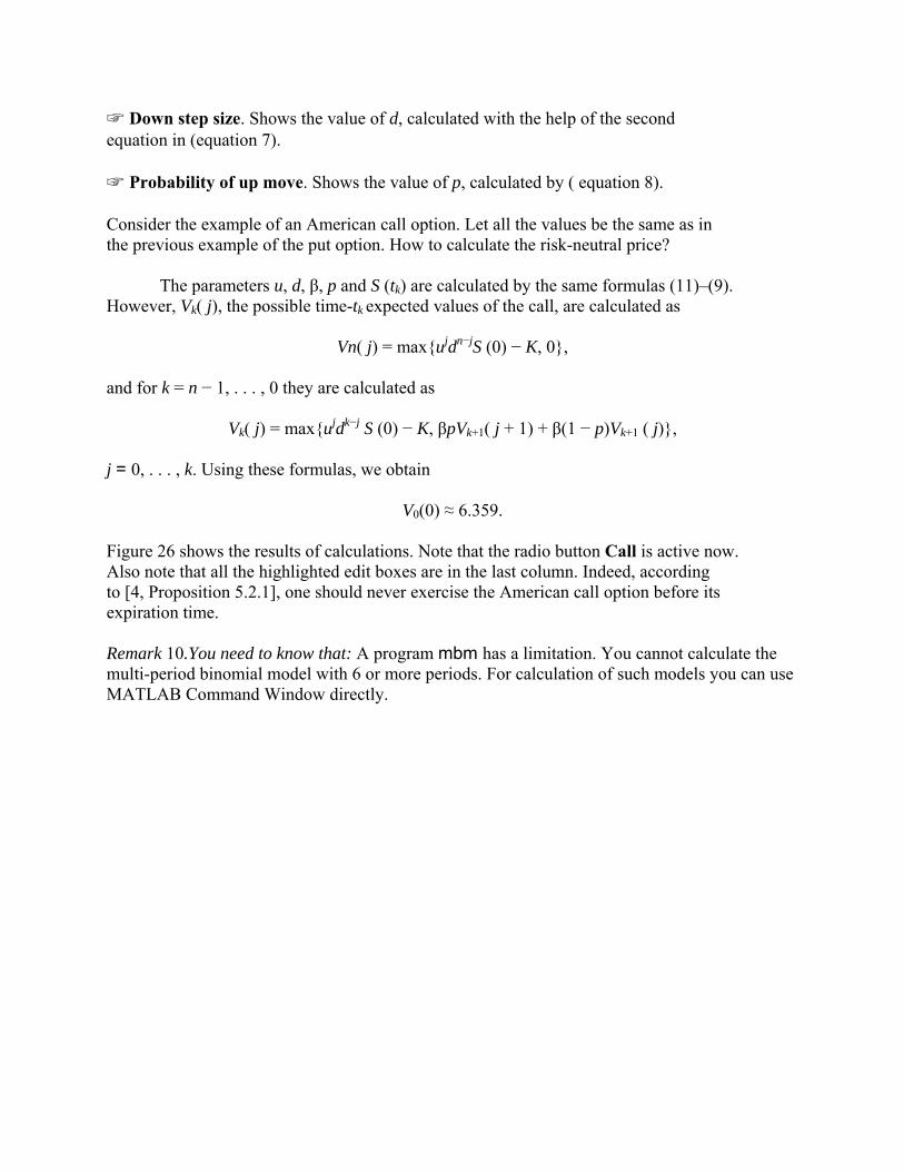
☞ Down step size. Shows the value of d, calculated with the help of the second equation in (equation 7). ☞ Probability of up move. Shows the value of p, calculated by ( equation 8). Consider the example of an American call option. Let all the values be the same as in the previous example of the put option. How to calculate the risk-neutral price? The parameters u, d, β, p and S (tk) are calculated by the same formulas (11)–(9). However, Vk( j), the possible time-tk expected values of the call, are calculated as
Vn( j) = max{ujdn−jS (0) − K, 0}, and for k = n − 1, . . . , 0 they are calculated as
Vk( j) = max{ujdk−j S (0) − K, βpVk+1( j + 1) + β(1 − p)Vk+1 ( j)},
j = 0, . . . , k. Using these formulas, we obtain
V0(0) ≈ 6.359. Figure 26 shows the results of calculations. Note that the radio button Call is active now. Also note that all the highlighted edit boxes are in the last column. Indeed, according to [4, Proposition 5.2.1], one should never exercise the American call option before its expiration time. Remark 10.You need to know that: A program mbm has a limitation. You cannot calculate the multi-period binomial model with 6 or more periods. For calculation of such models you can use MATLAB Command Window directly.
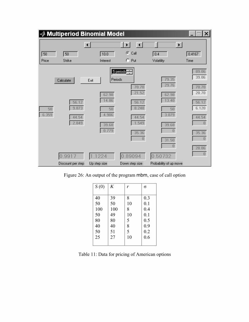
Figure 26: An output of the program mbm, case of call option
S (0) K r σ
40 50 100 50 80 40 50 25
39 50 100 49 80 40 51 27
8 10 8 10 5 8 5 10
0.3 0.1 0.4 0.1 0.5 0.9 0.2 0.6
Table 11: Data for pricing of American options
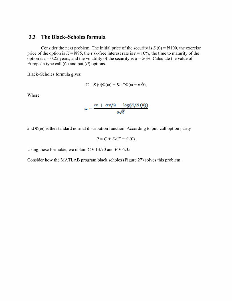
3.3 The Black–Scholes formula
Consider the next problem. The initial price of the security is S (0) = ₦100, the exercise price of the option is K = ₦95, the risk-free interest rate is r = 10%, the time to maturity of the option is t = 0.25 years, and the volatility of the security is σ = 50%. Calculate the value of European type call (C) and put (P) options. Black–Scholes formula gives
C = S (0)Φ(ω) − Ke−rtΦ(ω − σ√t),
Where
and Φ(ω) is the standard normal distribution function. According to put–call option parity
P = C + Ke−rt − S (0). Using these formulae, we obtain C ≈ 13.70 and P ≈ 6.35. Consider how the MATLAB program black scholes (Figure 27) solves this problem.
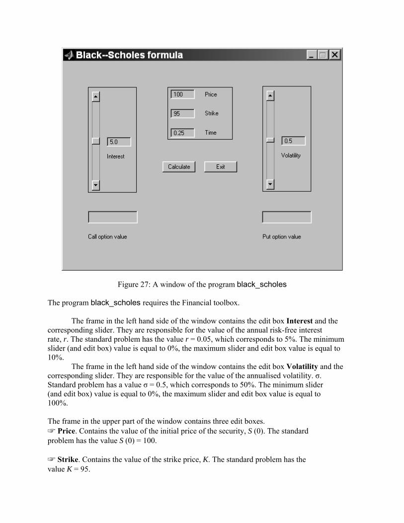
Figure 27: A window of the program black_scholes The program black_scholes requires the Financial toolbox.
The frame in the left hand side of the window contains the edit box Interest and the corresponding slider. They are responsible for the value of the annual risk-free interest rate, r. The standard problem has the value r = 0.05, which corresponds to 5%. The minimum slider (and edit box) value is equal to 0%, the maximum slider and edit box value is equal to 10%.
The frame in the left hand side of the window contains the edit box Volatility and the corresponding slider. They are responsible for the value of the annualised volatility. σ. Standard problem has a value σ = 0.5, which corresponds to 50%. The minimum slider (and edit box) value is equal to 0%, the maximum slider and edit box value is equal to 100%. The frame in the upper part of the window contains three edit boxes. ☞ Price. Contains the value of the initial price of the security, S (0). The standard problem has the value S (0) = 100. ☞ Strike. Contains the value of the strike price, K. The standard problem has the value K = 95.
☞ Time. Contains the time to maturity of the option in years, t. The standard problem has value t = 0.25. The push buttons perform the following functions. ☞ Calculate. Calculates values of call and put options, using the Black-Scholes formula and put-call option parity. ☞ Exit. Stops the program. The results of calculations of our example are shown on Figure 28. The disabled edit box Call option value contains the value of the call option, C. The disabled edit box Put option value contains the value of a put option, P. Exercise 1.. Calculate the value of call and put options for the cases from Table 11. The time to maturity of the option is t = 0.4167 years.
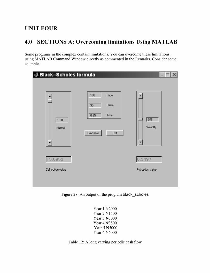
UNIT FOUR 4.0 SECTIONS A: Overcoming limitations Using MATLAB Some programs in the complex contain limitations. You can overcome these limitations, using MATLAB Command Window directly as commented in the Remarks. Consider some examples.
Figure 28: An output of the program black_scholes
Year 1 ₦2000 Year 2 ₦1500 Year 3 ₦3000 Year 4 ₦3800 Year 5 ₦5000 Year 6 ₦6000
Table 12: A long varying periodic cash flow
4.1 A.1: The program present_value Using the program present_value, you cannot calculate the present value of a cash flow containing more than 5 payments. The Command Window can be used instead. Consider the next example.
The cash flow (Table 12) represents the yearly income from an initial investment of $15,000. The annual interest rate is 8%. How to calculate the present value of this varying cash flow?
We cannot use the program present_value directly, because our cash flow contains more than 5 payments. Instead we can make direct use of the MATLAB Command Window.
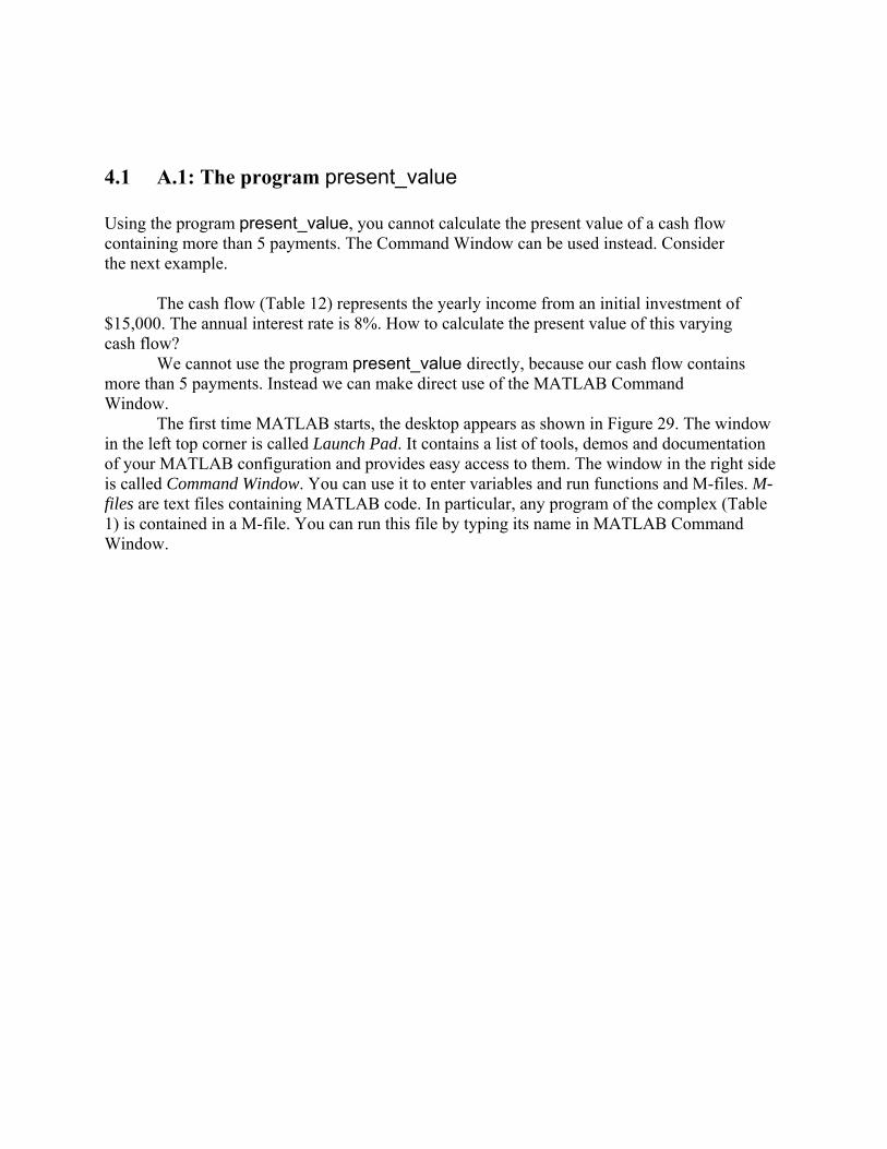
The first time MATLAB starts, the desktop appears as shown in Figure 29. The window in the left top corner is called Launch Pad. It contains a list of tools, demos and documentation of your MATLAB configuration and provides easy access to them. The window in the right side is called Command Window. You can use it to enter variables and run functions and M-files. M-files are text files containing MATLAB code. In particular, any program of the complex (Table 1) is contained in a M-file. You can run this file by typing its name in MATLAB Command Window.
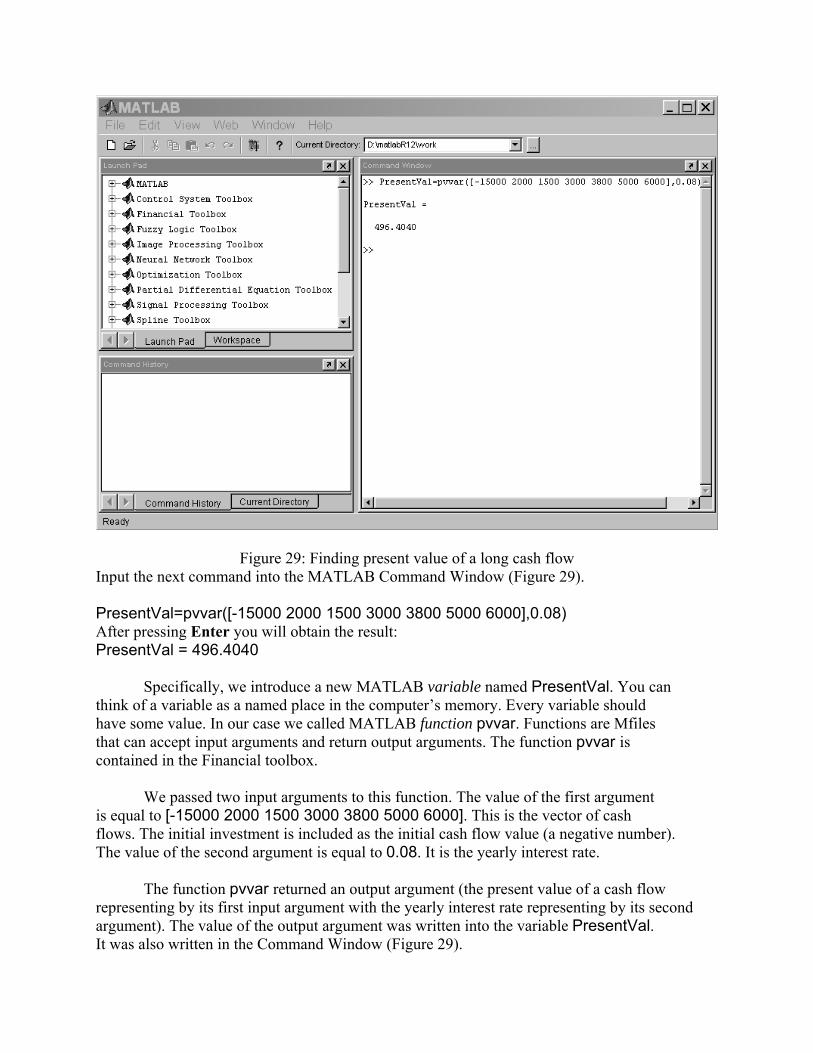
Figure 29: Finding present value of a long cash flow Input the next command into the MATLAB Command Window (Figure 29). PresentVal=pvvar([-15000 2000 1500 3000 3800 5000 6000],0.08) After pressing Enter you will obtain the result: PresentVal = 496.4040
Specifically, we introduce a new MATLAB variable named PresentVal. You can think of a variable as a named place in the computer’s memory. Every variable should have some value. In our case we called MATLAB function pvvar. Functions are Mfiles that can accept input arguments and return output arguments. The function pvvar is contained in the Financial toolbox.
We passed two input arguments to this function. The value of the first argument is equal to [-15000 2000 1500 3000 3800 5000 6000]. This is the vector of cash flows. The initial investment is included as the initial cash flow value (a negative number). The value of the second argument is equal to 0.08. It is the yearly interest rate.
The function pvvar returned an output argument (the present value of a cash flow representing by its first input argument with the yearly interest rate representing by its second argument). The value of the output argument was written into the variable PresentVal. It was also written in the Command Window (Figure 29).
4.2 A.2 The program ror Using the program ror, you cannot calculate the rate of return of a cash flow containing more than 5 payments. The Command Window can be used instead.
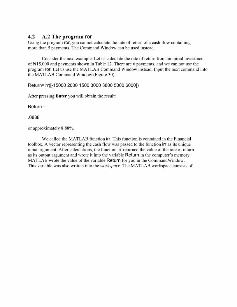
Consider the next example. Let us calculate the rate of return from an initial investment of ₦15,000 and payments shown in Table 12. There are 6 payments, and we can not use the program ror. Let us use the MATLAB Command Window instead. Input the next command into the MATLAB Command Window (Figure 30). Return=irr([-15000 2000 1500 3000 3800 5000 6000]) After pressing Enter you will obtain the result: Return = .0888 or approximately 8.88%.
We called the MATLAB function irr. This function is contained in the Financial toolbox. A vector representing the cash flow was passed to the function irr as its unique input argument. After calculations, the function irr returned the value of the rate of return as its output argument and wrote it into the variable Return in the computer’s memory. MATLAB wrote the value of the variable Return for you in the CommandWindow. This variable was also written into the workspace. The MATLAB workspace consists of
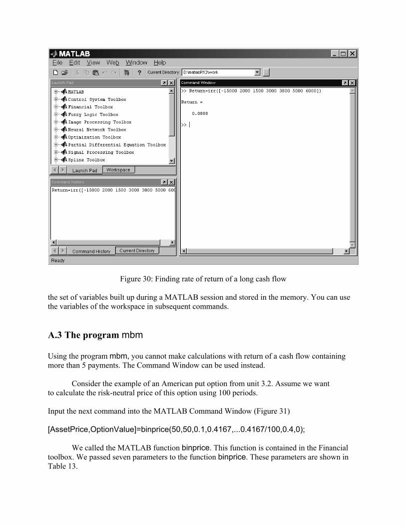
Figure 30: Finding rate of return of a long cash flow the set of variables built up during a MATLAB session and stored in the memory. You can use the variables of the workspace in subsequent commands. A.3 The program mbm Using the program mbm, you cannot make calculations with return of a cash flow containing more than 5 payments. The Command Window can be used instead.
Consider the example of an American put option from unit 3.2. Assume we want to calculate the risk-neutral price of this option using 100 periods. Input the next command into the MATLAB Command Window (Figure 31) [AssetPrice,OptionValue]=binprice(50,50,0.1,0.4167,...0.4167/100,0.4,0);
We called the MATLAB function binprice. This function is contained in the Financial toolbox. We passed seven parameters to the function binprice. These parameters are shown in Table 13.
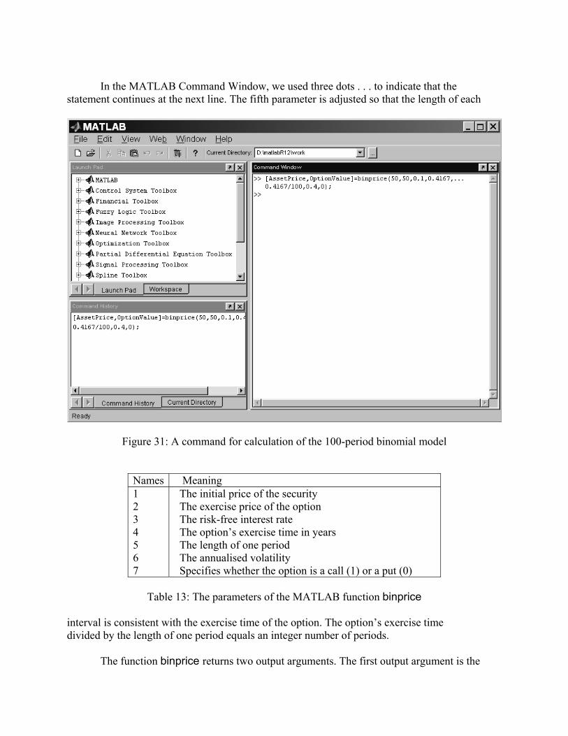
In the MATLAB Command Window, we used three dots . . . to indicate that the
statement continues at the next line. The fifth parameter is adjusted so that the length of each
Figure 31: A command for calculation of the 100-period binomial model
Names Meaning 1 2 3 4 5 6 7
The initial price of the security The exercise price of the option The risk-free interest rate The option’s exercise time in years The length of one period The annualised volatility Specifies whether the option is a call (1) or a put (0)
Table 13: The parameters of the MATLAB function binprice
interval is consistent with the exercise time of the option. The option’s exercise time divided by the length of one period equals an integer number of periods.
The function binprice returns two output arguments. The first output argument is the
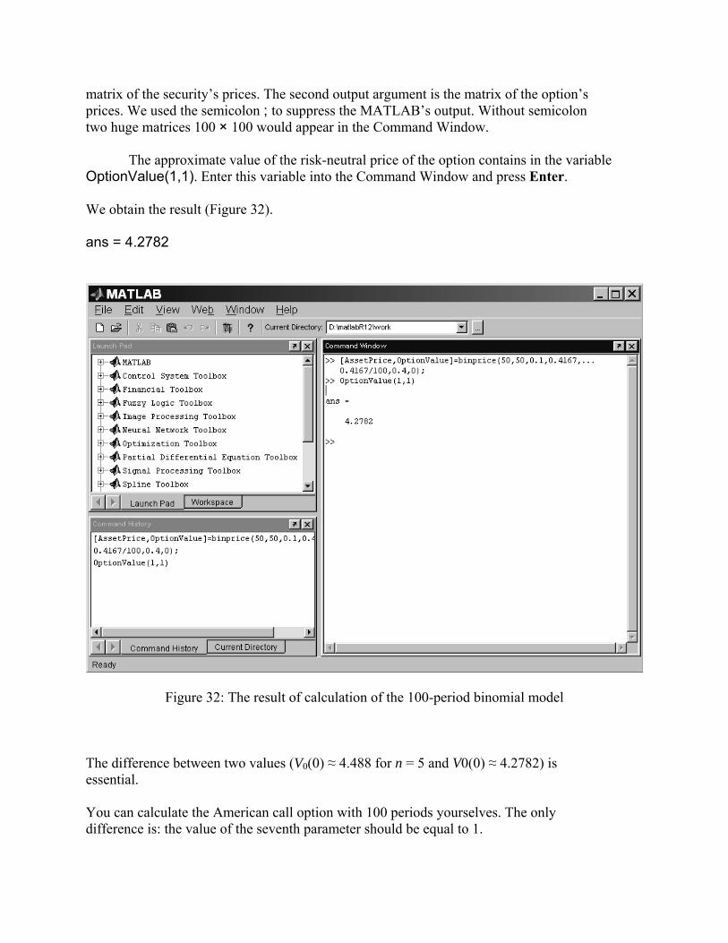
matrix of the security’s prices. The second output argument is the matrix of the option’s prices. We used the semicolon ; to suppress the MATLAB’s output. Without semicolon two huge matrices 100 × 100 would appear in the Command Window.
The approximate value of the risk-neutral price of the option contains in the variable OptionValue(1,1). Enter this variable into the Command Window and press Enter. We obtain the result (Figure 32). ans = 4.2782
Figure 32: The result of calculation of the 100-period binomial model
The difference between two values (V0(0) ≈ 4.488 for n = 5 and V0(0) ≈ 4.2782) is essential. You can calculate the American call option with 100 periods yourselves. The only difference is: the value of the seventh parameter should be equal to 1.

Exercise 1. Calculate the value of call and put options for the cases from Table 11. The time to maturity of the option is t = 0.4167 years. Divide it onto 100 equal parts. References [1] Financial Toolbox for Use with MATLAB, User’s Guide, Version 2.1.2, The Math- Works, Inc., September 2000. [2] Hull, J. C. Options, Futures & Other Derivatives, Fourth Edition, Prentice Hall, Upper Saddle River, 2000. [3] Prisman, E. Z. Pricing Derivative Securities: an Interactive Dynamic Environment with Maple V and Matlab, Academic Press, 2000. [4] Ross, S. M. An introduction to Mathematical Finance: Options and Other Topics, Cambridge University Press, 1999. [5] Google Inc.;www.google.com [6 Investopedia.com ,Inc.; www.investopedia.com
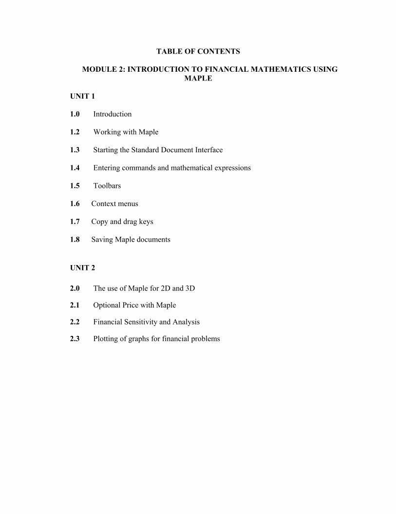
TABLE OF CONTENTS
MODULE 2: INTRODUCTION TO FINANCIAL MATHEMATICS USING MAPLE
UNIT 1 1.0 Introduction
1.2 Working with Maple
1.3 Starting the Standard Document Interface
1.4 Entering commands and mathematical expressions
1.5 Toolbars
1.6 Context menus
1.7 Copy and drag keys
1.8 Saving Maple documents UNIT 2 2.0 The use of Maple for 2D and 3D
2.1 Optional Price with Maple
2.2 Financial Sensitivity and Analysis
2.3 Plotting of graphs for financial problems
1.0 Introduction Maple is a powerful mathematical computer program, designed to perform a wide variety of mathematical calculations and operations. It can do simple calculations, matrix operations, graphing, and even symbolic manipulations, such as finding the derivative or integral of a function. It can also solve a variety of equations such as finding zeros of a polynomial or to solve linear as well as some nonlinear systems of equations.
Maple™ is a powerful software that can be used to solve mathematical problems from simple to complex. You can also create professional quality documents, presentations, and custom computational interactive tools in Maple environments. Mathematics touches us every day from the simple chore of calculating the total cost of our purchases to the complex calculations used to construct the bridges we travel. To harness the power of mathematics, Maplesoft, provides a tool in an accessible and complete form. That tool is Maple. 1.1 Objectives
By the end of this unit, you should be able to:
Understand Maple environment Know how to start the Standard Document Interface Understand how to enter commands and mathematical expressions in Maple Understand MapleToolbars Understand and how to use Context menus Know how to use Copy and drag keys How to save Maple documents

1.2 WORKING WITH MAPLE
With Maple, you can create powerful interactive documents. The Maple environment lets you start solving problems right away by entering expressions in 2-D Math and solving these expressions using point-and-click inter-faces. You can combine text and math in the same line, add tables to organize the content of your work, or insert images, sketch regions, and spreadsheets. You can visualize and animate problems in two and three dimensions, format text for academic papers or books, and insert hyperlinks to other Maple files, web sites, or email addresses. You can embed and program graphical user interface components, as well as devise custom solutions using the Maple programming language. You can access the power of the Maple computational engine through a variety of interfaces as explained in the table below:
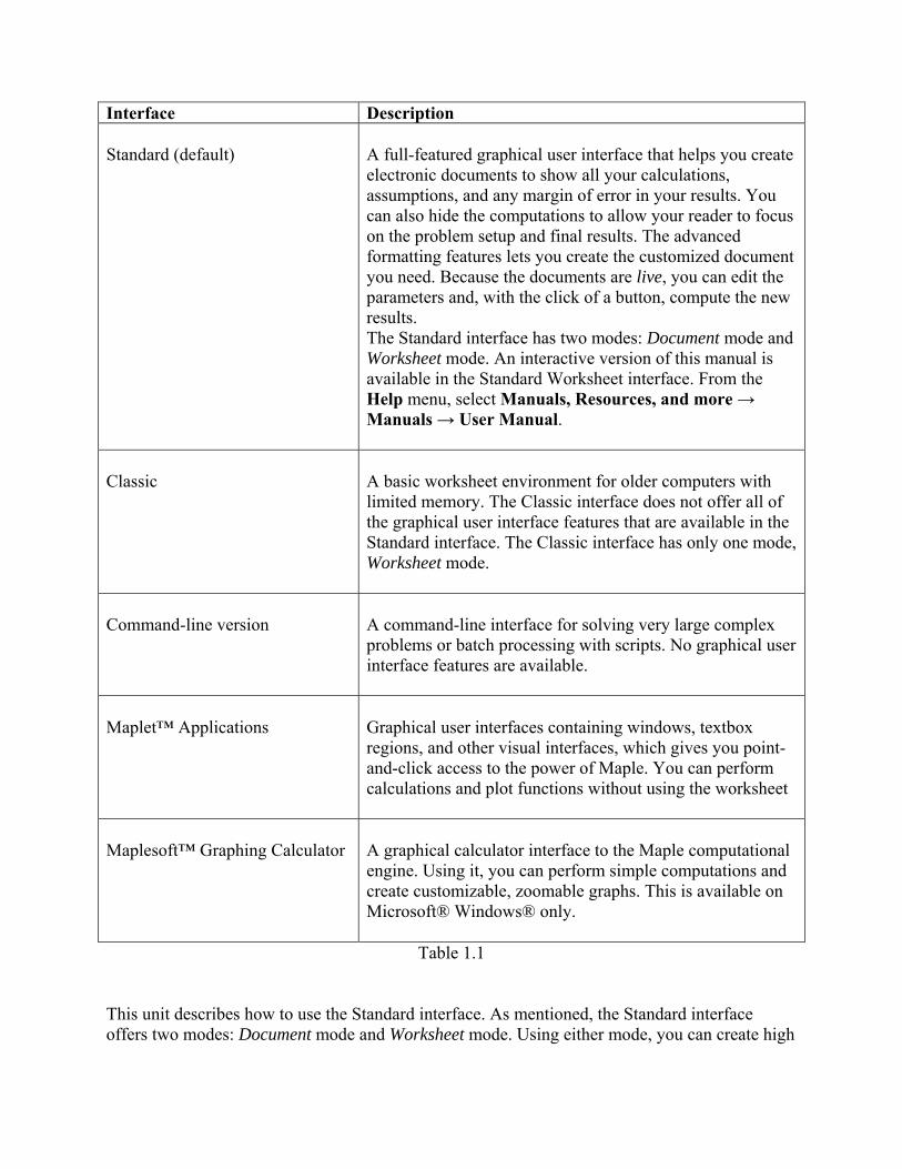
Table 1.1
This unit describes how to use the Standard interface. As mentioned, the Standard interface offers two modes: Document mode and Worksheet mode. Using either mode, you can create high
Interface Description Standard (default)
A full-featured graphical user interface that helps you create electronic documents to show all your calculations, assumptions, and any margin of error in your results. You can also hide the computations to allow your reader to focus on the problem setup and final results. The advanced formatting features lets you create the customized document you need. Because the documents are live, you can edit the parameters and, with the click of a button, compute the new results. The Standard interface has two modes: Document mode and Worksheet mode. An interactive version of this manual is available in the Standard Worksheet interface. From the Help menu, select Manuals, Resources, and more → Manuals → User Manual.
Classic
A basic worksheet environment for older computers with limited memory. The Classic interface does not offer all of the graphical user interface features that are available in the Standard interface. The Classic interface has only one mode, Worksheet mode.
Command-line version
A command-line interface for solving very large complex problems or batch processing with scripts. No graphical user interface features are available.
Maplet™ Applications
Graphical user interfaces containing windows, textbox regions, and other visual interfaces, which gives you point-and-click access to the power of Maple. You can perform calculations and plot functions without using the worksheet
Maplesoft™ Graphing Calculator
A graphical calculator interface to the Maple computational engine. Using it, you can perform simple computations and create customizable, zoomable graphs. This is available on Microsoft® Windows® only.
quality interactive mathematical documents. Each mode offers the same features and functionality, the only difference is the default input region of each mode. You will be introduced to some other parts of the application as you continue in your study of Financial Mathematics. Shortcut Keys by Platform This manual will frequently refer to context menus and command completion when entering expressions. The keyboard keys used to invoke these features differ based on your operating system. This unit will only refer to the keyboard keys needed for a Windows operating system.
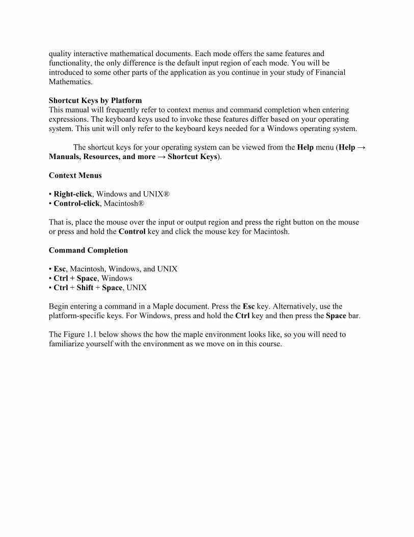
The shortcut keys for your operating system can be viewed from the Help menu (Help → Manuals, Resources, and more → Shortcut Keys). Context Menus • Right-click, Windows and UNIX® • Control-click, Macintosh® That is, place the mouse over the input or output region and press the right button on the mouse or press and hold the Control key and click the mouse key for Macintosh. Command Completion • Esc, Macintosh, Windows, and UNIX • Ctrl + Space, Windows • Ctrl + Shift + Space, UNIX Begin entering a command in a Maple document. Press the Esc key. Alternatively, use the platform-specific keys. For Windows, press and hold the Ctrl key and then press the Space bar. The Figure 1.1 below shows the how the maple environment looks like, so you will need to familiarize yourself with the environment as we move on in this course.
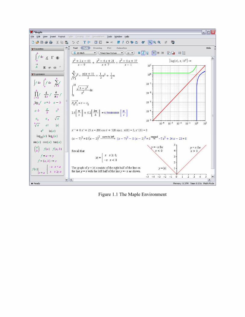
Figure 1.1 The Maple Environment
1.3 STARTING THE STANDARD DOCUMENT INTERFACE To start Maple on: Windows
From the Start menu, select All Programs → Maple 17 → Maple 17. Alternatively: Double-click the Maple 17 desktop icon.
Macintosh
1. From the Finder, select Applications and Maple 17. 2. Double-click Maple 17.
UNIX
Enter the full path, for example, /usr/local/maple/bin/xmaple Alternatively:
1. Add the Maple directory (for example, /usr/local/maple/bin) to your command search path.
2. Enter xmaple.
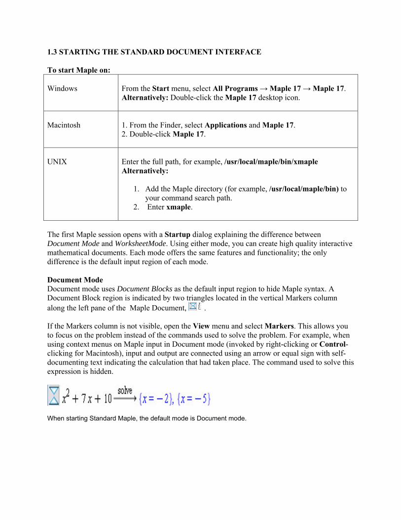
The first Maple session opens with a Startup dialog explaining the difference between Document Mode and WorksheetMode. Using either mode, you can create high quality interactive mathematical documents. Each mode offers the same features and functionality; the only difference is the default input region of each mode. Document Mode Document mode uses Document Blocks as the default input region to hide Maple syntax. A Document Block region is indicated by two triangles located in the vertical Markers column along the left pane of the Maple Document, . If the Markers column is not visible, open the View menu and select Markers. This allows you to focus on the problem instead of the commands used to solve the problem. For example, when using context menus on Maple input in Document mode (invoked by right-clicking or Control-clicking for Macintosh), input and output are connected using an arrow or equal sign with self-documenting text indicating the calculation that had taken place. The command used to solve this expression is hidden.
When starting Standard Maple, the default mode is Document mode.
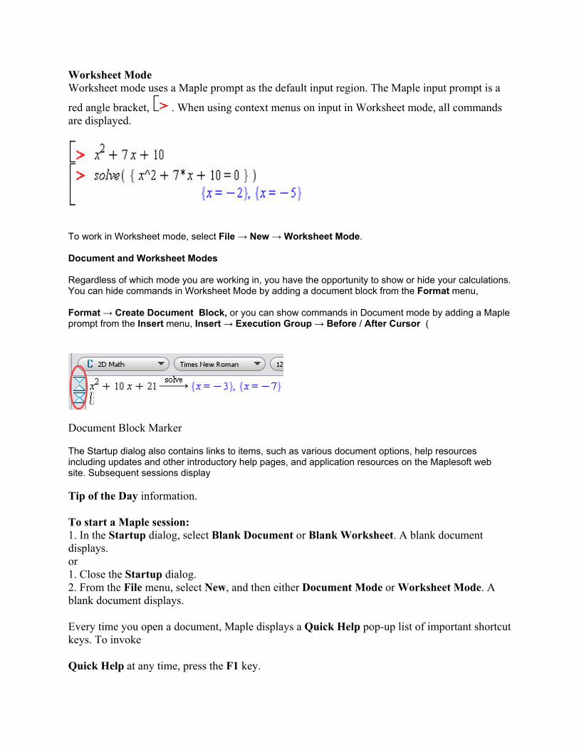
Worksheet Mode Worksheet mode uses a Maple prompt as the default input region. The Maple input prompt is a
red angle bracket, . When using context menus on input in Worksheet mode, all commands are displayed.
To work in Worksheet mode, select File → New → Worksheet Mode. Document and Worksheet Modes Regardless of which mode you are working in, you have the opportunity to show or hide your calculations. You can hide commands in Worksheet Mode by adding a document block from the Format menu, Format → Create Document Block, or you can show commands in Document mode by adding a Maple prompt from the Insert menu, Insert → Execution Group → Before / After Cursor (
Document Block Marker
The Startup dialog also contains links to items, such as various document options, help resources including updates and other introductory help pages, and application resources on the Maplesoft web site. Subsequent sessions display Tip of the Day information. To start a Maple session: 1. In the Startup dialog, select Blank Document or Blank Worksheet. A blank document displays. or 1. Close the Startup dialog. 2. From the File menu, select New, and then either Document Mode or Worksheet Mode. A blank document displays. Every time you open a document, Maple displays a Quick Help pop-up list of important shortcut keys. To invoke Quick Help at any time, press the F1 key.
1.4 ENTERING COMMMANDS AND MATHEMATICAL EXPRESSION
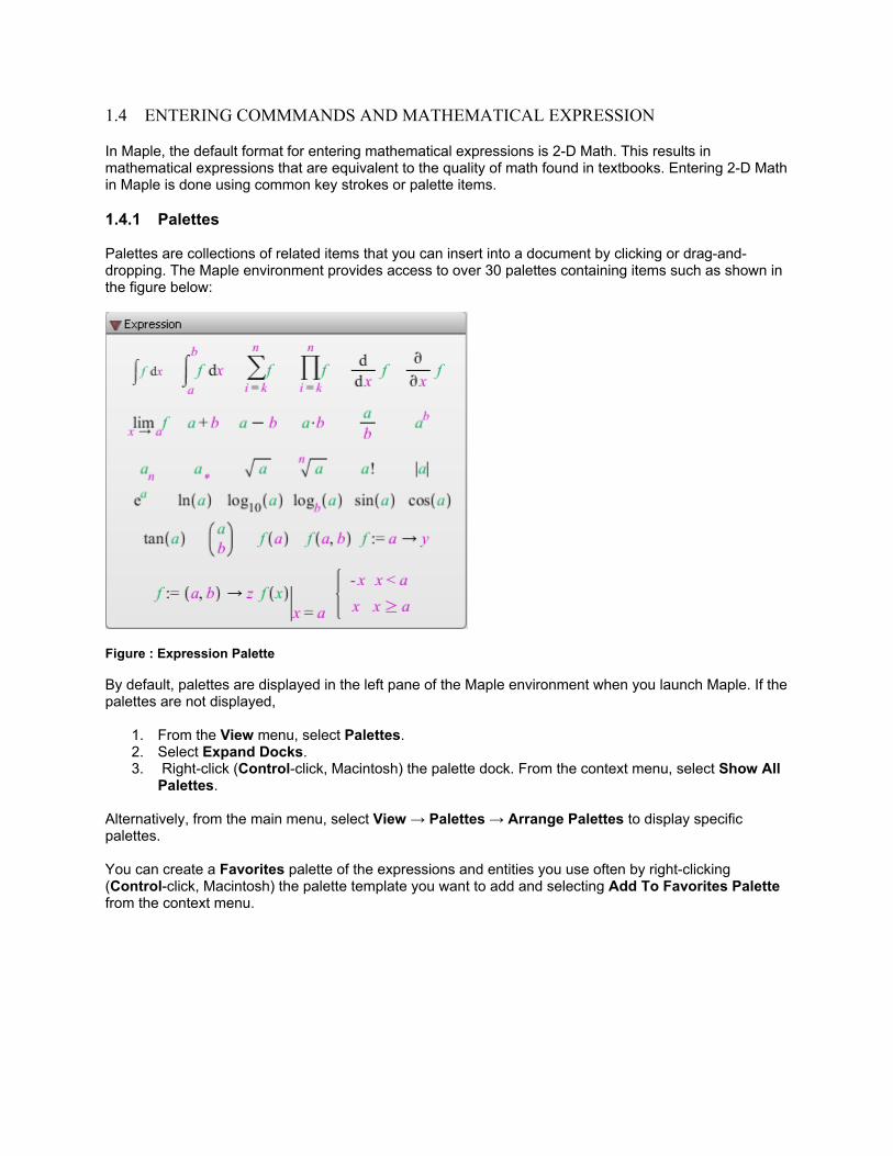
In Maple, the default format for entering mathematical expressions is 2-D Math. This results in mathematical expressions that are equivalent to the quality of math found in textbooks. Entering 2-D Math in Maple is done using common key strokes or palette items. 1.4.1 Palettes
Palettes are collections of related items that you can insert into a document by clicking or drag-and-dropping. The Maple environment provides access to over 30 palettes containing items such as shown in the figure below:
Figure : Expression Palette By default, palettes are displayed in the left pane of the Maple environment when you launch Maple. If the palettes are not displayed,
1. From the View menu, select Palettes. 2. Select Expand Docks. 3. Right-click (Control-click, Macintosh) the palette dock. From the context menu, select Show All
Palettes. Alternatively, from the main menu, select View → Palettes → Arrange Palettes to display specific palettes. You can create a Favorites palette of the expressions and entities you use often by right-clicking (Control-click, Macintosh) the palette template you want to add and selecting Add To Favorites Palette from the context menu.
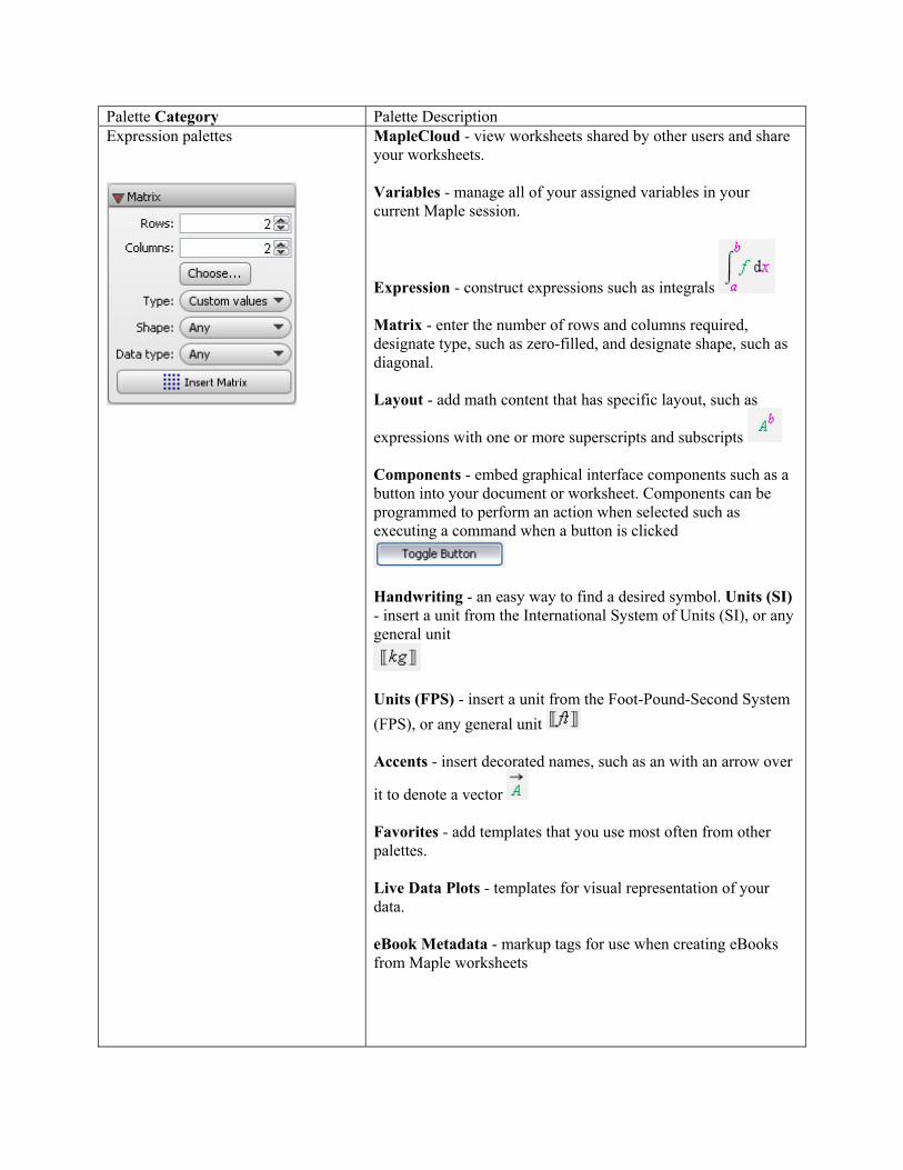
Palette Category Palette Description Expression palettes
MapleCloud - view worksheets shared by other users and share your worksheets. Variables - manage all of your assigned variables in your current Maple session.
Expression - construct expressions such as integrals Matrix - enter the number of rows and columns required, designate type, such as zero-filled, and designate shape, such as diagonal. Layout - add math content that has specific layout, such as
expressions with one or more superscripts and subscripts
Components - embed graphical interface components such as a button into your document or worksheet. Components can be programmed to perform an action when selected such as executing a command when a button is clicked
Handwriting - an easy way to find a desired symbol. Units (SI) - insert a unit from the International System of Units (SI), or any general unit
Units (FPS) - insert a unit from the Foot-Pound-Second System
(FPS), or any general unit Accents - insert decorated names, such as an with an arrow over
it to denote a vector Favorites - add templates that you use most often from other palettes. Live Data Plots - templates for visual representation of your data. eBook Metadata - markup tags for use when creating eBooks from Maple worksheets
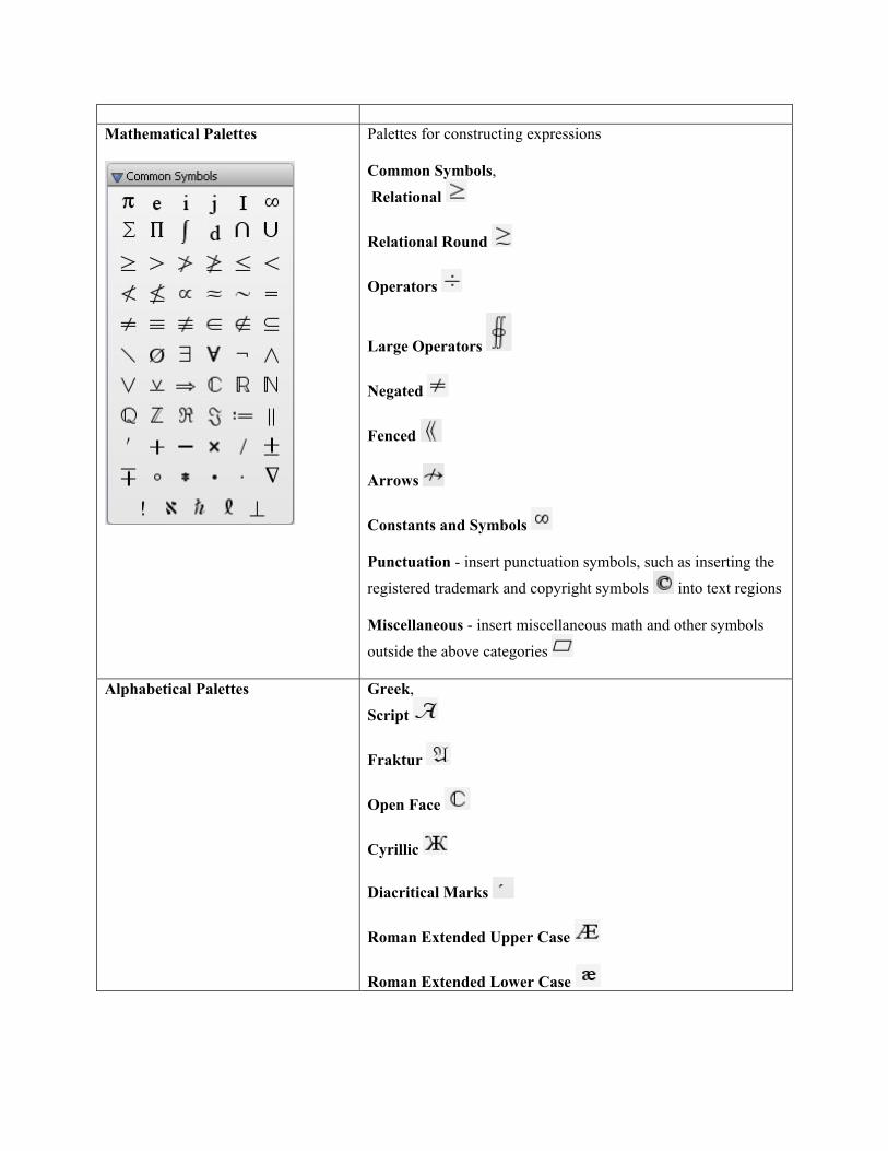
Mathematical Palettes
Palettes for constructing expressions Common Symbols,
Relational
Relational Round
Operators
Large Operators
Negated
Fenced
Arrows
Constants and Symbols Punctuation - insert punctuation symbols, such as inserting the
registered trademark and copyright symbols into text regions Miscellaneous - insert miscellaneous math and other symbols
outside the above categories
Alphabetical Palettes
Greek,
Script
Fraktur
Open Face
Cyrillic
Diacritical Marks
Roman Extended Upper Case
Roman Extended Lower Case
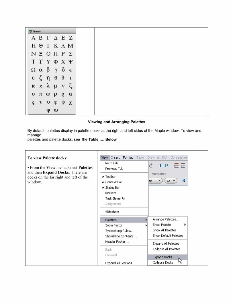
Viewing and Arranging Palettes
By default, palettes display in palette docks at the right and left sides of the Maple window. To view and manage palettes and palette docks, see the Table …. Below To view Palette docks: • From the View menu, select Palettes, and then Expand Docks. There are docks on the far right and left of the window.
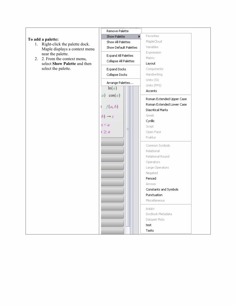
To add a palette:
1. Right-click the palette dock. Maple displays a context menu near the palette.
2. 2. From the context menu, select Show Palette and then
select the palette.
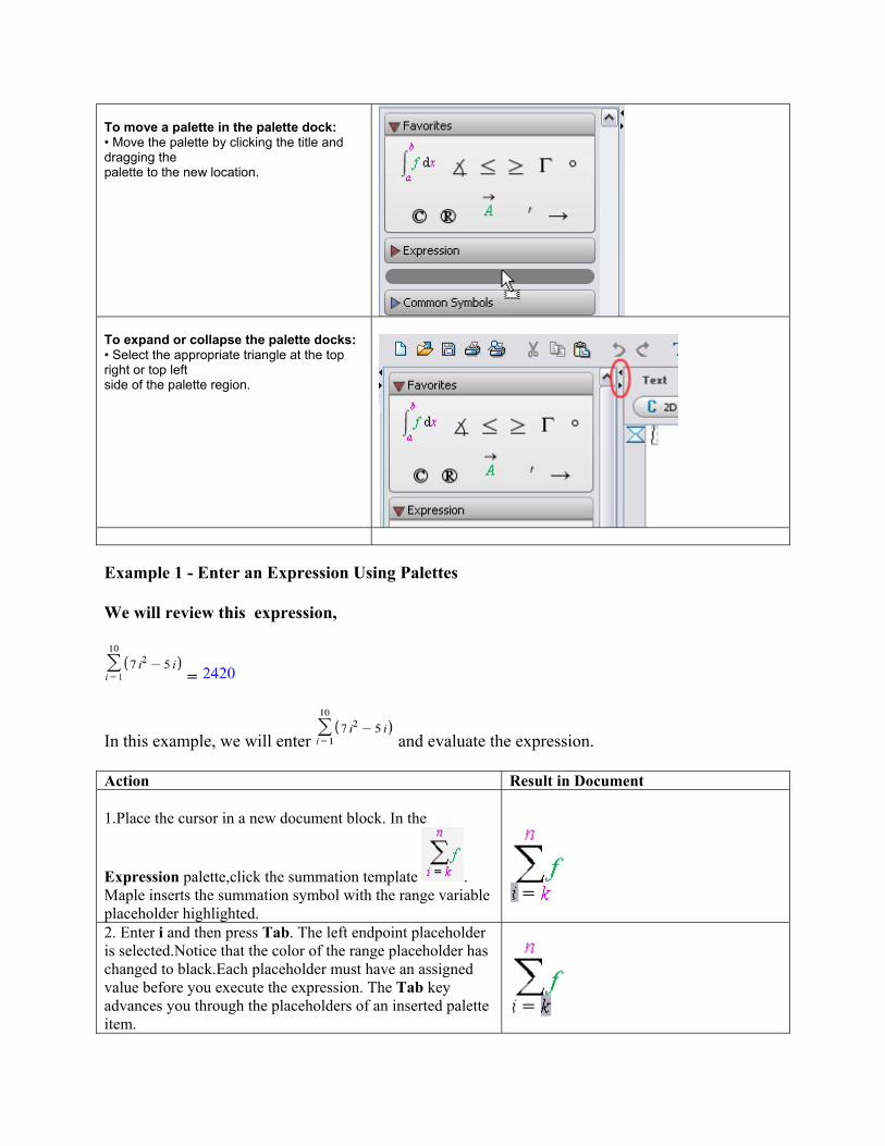
To move a palette in the palette dock: • Move the palette by clicking the title and dragging the palette to the new location.
To expand or collapse the palette docks: • Select the appropriate triangle at the top right or top left side of the palette region.
Example 1 - Enter an Expression Using Palettes We will review this expression,
=
In this example, we will enter and evaluate the expression. Action Result in Document 1.Place the cursor in a new document block. In the
Expression palette,click the summation template . Maple inserts the summation symbol with the range variable placeholder highlighted.
2. Enter i and then press Tab. The left endpoint placeholder is selected.Notice that the color of the range placeholder has changed to black.Each placeholder must have an assigned value before you execute the expression. The Tab key advances you through the placeholders of an inserted palette item.
Action Result in Document 3. Enter 1 and then press Tab. The right endpoint placeholder is selected
4. Enter 10 and then press Tab. The expression placeholder is selected
5. Enter For instructions on entering this type of expression,
see Example 1 - Enter and Evaluate an Expression Using Keystrokes (page 5).
6. Press Ctrl + = (Command + = for Macintosh) to evaluate the summation
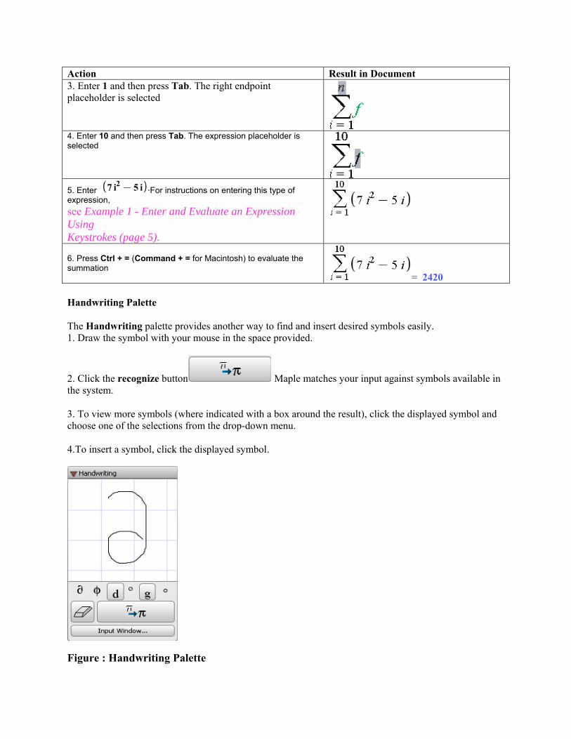
= 2420 Handwriting Palette The Handwriting palette provides another way to find and insert desired symbols easily. 1. Draw the symbol with your mouse in the space provided.
2. Click the recognize button Maple matches your input against symbols available in the system. 3. To view more symbols (where indicated with a box around the result), click the displayed symbol and choose one of the selections from the drop-down menu.
4.To insert a symbol, click the displayed symbol.
Figure : Handwriting Palette
Snippets Palettes You can create your own custom Snippets palettes for tasks that you find most useful. Details on how to create and customize Snippets palettes can be found on the createpalette help page. Common Operations in Maple
Entering mathematical expressions, such as, , and is natural in 2-D Math. To enter a fraction: 1. Enter the numerator. 2. Press the forward slash (/) key. 3. Enter the denominator. 4. To leave the denominator, press the right arrow key. To enter a power: 1. Enter the base. 2. Press the caret (^) key. 3. Enter the exponent, which displays in math as a superscript. 4. To leave the exponent, press the right arrow key. To enter a product: 1. Enter the first factor. 2. Press the asterisk (*) key, which displays in 2-D Math as a dot, . 3. Enter the second factor. Implied Multiplication: In most cases, you do not need to include the multiplication operator, . Insert a space character between two quantities to multiply them. Note: In some cases, you do not need to enter the multiplication operator or a space character. For example, Maple interprets a number followed by a variable as multiplication. Important: Maple interprets a sequence of letters, for example, xy, as a single variable. To specify the product of two variables, you must insert a space character (or multiplication operator), for example, x y or
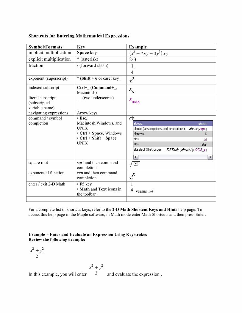
Shortcuts for Entering Mathematical Expressions Symbol/Formats Key Exampleimplicit multiplication Space key explicit multiplication * (asterisk) fraction / (forward slash)
exponent (superscript) ^ (Shift + 6 or caret key)
indexed subscript Ctrl+_ (Command+_, Macintosh)
literal subscript (subscripted variable name)
__ (two underscores)
navigating expressions Arrow keys command / symbol completion
• Esc, Macintosh,Windows, and UNIX • Ctrl + Space, Windows • Ctrl + Shift + Space, UNIX
square root sqrt and then command completion
exponential function exp and then command completion
enter / exit 2-D Math • F5 key • Math and Text icons in the toolbar
versus 1/4
For a complete list of shortcut keys, refer to the 2-D Math Shortcut Keys and Hints help page. To access this help page in the Maple software, in Math mode enter Math Shortcuts and then press Enter. Example - Enter and Evaluate an Expression Using Keystrokes Review the following example:
In this example, you will enter and evaluate the expression ,
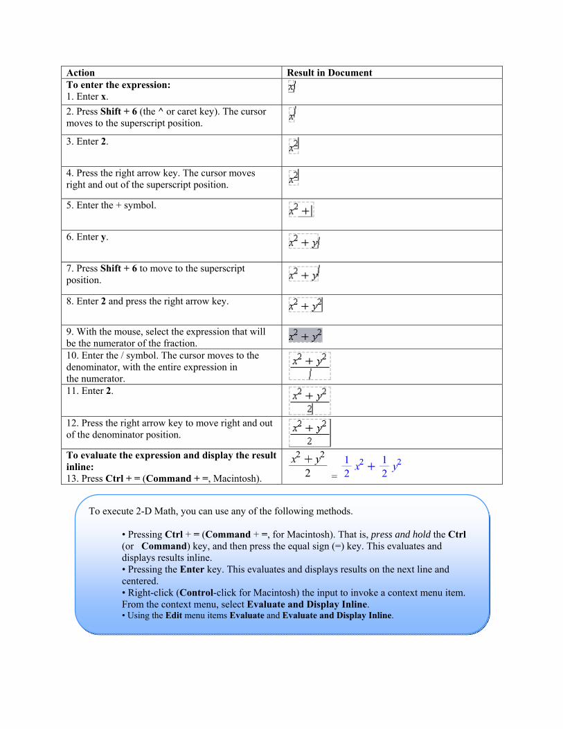
Action Result in Document To enter the expression: 1. Enter x.
2. Press Shift + 6 (the ^ or caret key). The cursor moves to the superscript position.
3. Enter 2.
4. Press the right arrow key. The cursor moves right and out of the superscript position.
5. Enter the + symbol.
6. Enter y.
7. Press Shift + 6 to move to the superscript position.
8. Enter 2 and press the right arrow key.
9. With the mouse, select the expression that will be the numerator of the fraction.
10. Enter the / symbol. The cursor moves to the denominator, with the entire expression in the numerator. 11. Enter 2.
12. Press the right arrow key to move right and out of the denominator position.
To evaluate the expression and display the result inline: 13. Press Ctrl + = (Command + =, Macintosh). =
To execute 2-D Math, you can use any of the following methods.
• Pressing Ctrl + = (Command + =, for Macintosh). That is, press and hold the Ctrl (or Command) key, and then press the equal sign (=) key. This evaluates and displays results inline. • Pressing the Enter key. This evaluates and displays results on the next line and centered. • Right-click (Control-click for Macintosh) the input to invoke a context menu item. From the context menu, select Evaluate and Display Inline. • Using the Edit menu items Evaluate and Evaluate and Display Inline.
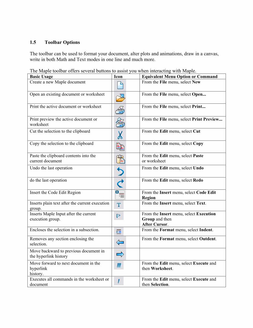
1.5 Toolbar Options The toolbar can be used to format your document, alter plots and animations, draw in a canvas, write in both Math and Text modes in one line and much more. The Maple toolbar offers several buttons to assist you when interacting with Maple. Basic Usage Icon Equivalent Menu Option or CommandCreate a new Maple document From the File menu, select New
Open an existing document or worksheet From the File menu, select Open...
Print the active document or worksheet From the File menu, select Print...
Print preview the active document or worksheet
From the File menu, select Print Preview...
Cut the selection to the clipboard From the Edit menu, select Cut
Copy the selection to the clipboard From the Edit menu, select Copy
Paste the clipboard contents into the current document
From the Edit menu, select Paste or worksheet
Undo the last operation From the Edit menu, select Undo
do the last operation From the Edit menu, select Redo
Insert the Code Edit Region From the Insert menu, select Code Edit Region
Inserts plain text after the current execution group.
From the Insert menu, select Text.
Inserts Maple Input after the current execution group.
From the Insert menu, select Execution Group and then After Cursor.
Encloses the selection in a subsection. From the Format menu, select Indent.
Removes any section enclosing the selection.
From the Format menu, select Outdent.
Move backward to previous document in the hyperlink history
Move forward to next document in the hyperlink history.
From the Edit menu, select Execute and then Worksheet.
Executes all commands in the worksheet or document
From the Edit menu, select Execute and then Selection.
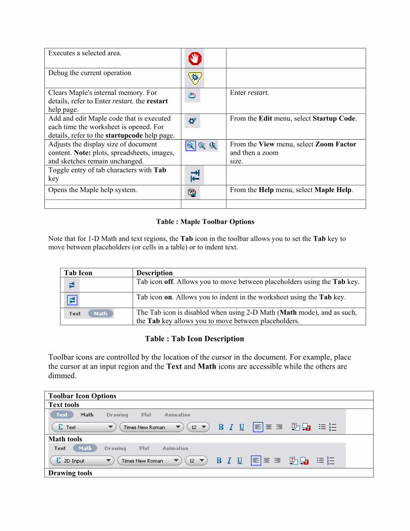
Executes a selected area.
Debug the current operation
Clears Maple's internal memory. For details, refer to Enter restart. the restart help page.
Enter restart.
Add and edit Maple code that is executed each time the worksheet is opened. For details, refer to the startupcode help page.
From the Edit menu, select Startup Code.
Adjusts the display size of document content. Note: plots, spreadsheets, images, and sketches remain unchanged.
From the View menu, select Zoom Factor and then a zoom size.
Toggle entry of tab characters with Tab key
Opens the Maple help system. From the Help menu, select Maple Help.
Table : Maple Toolbar Options
Note that for 1-D Math and text regions, the Tab icon in the toolbar allows you to set the Tab key to move between placeholders (or cells in a table) or to indent text.
Tab Icon Description
Tab icon off. Allows you to move between placeholders using the Tab key.
Tab icon on. Allows you to indent in the worksheet using the Tab key.
The Tab icon is disabled when using 2-D Math (Math mode), and as such, the Tab key allows you to move between placeholders.
Table : Tab Icon Description
Toolbar icons are controlled by the location of the cursor in the document. For example, place the cursor at an input region and the Text and Math icons are accessible while the others are dimmed.
Toolbar Icon Options Text tools
Math tools
Drawing tools
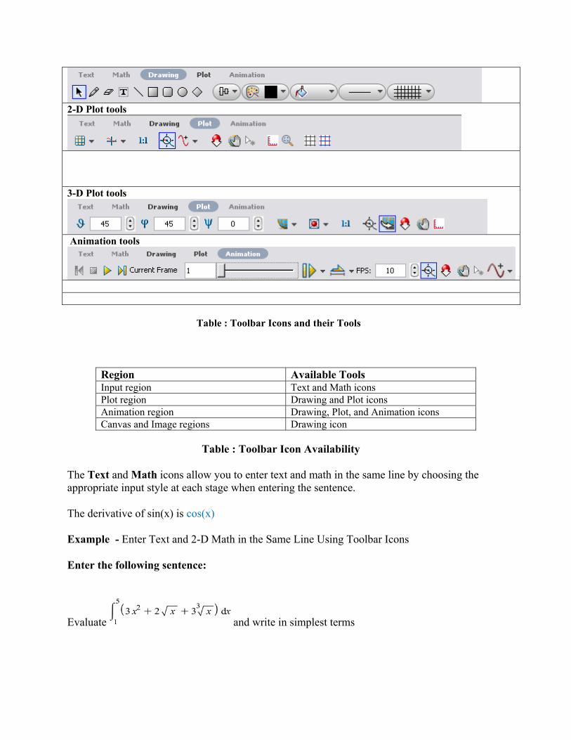
Table : Toolbar Icons and their Tools
Region Available Tools Input region Text and Math icons Plot region Drawing and Plot icons Animation region Drawing, Plot, and Animation icons Canvas and Image regions Drawing icon
Table : Toolbar Icon Availability
The Text and Math icons allow you to enter text and math in the same line by choosing the appropriate input style at each stage when entering the sentence. The derivative of sin(x) is cos(x) Example - Enter Text and 2-D Math in the Same Line Using Toolbar Icons Enter the following sentence:
Evaluate and write in simplest terms
2-D Plot tools
3-D Plot tools
Animation tools
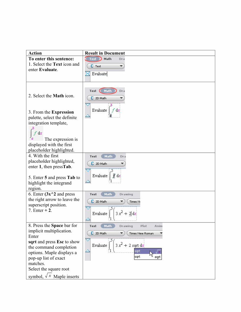
Action Result in DocumentTo enter this sentence: 1. Select the Text icon and enter Evaluate.
2. Select the Math icon. 3. From the Expression palette, select the definite integration template,
The expression is displayed with the first placeholder highlighted.
4. With the first placeholder highlighted, enter 1, then pressTab. 5. Enter 5 and press Tab to highlight the integrand region.
6. Enter (3x^2 and press the right arrow to leave the superscript position. 7. Enter + 2.
8. Press the Space bar for implicit multiplication. Enter sqrt and press Esc to show the command completion options. Maple displays a pop-up list of exact matches. Select the square root
symbol, Maple inserts
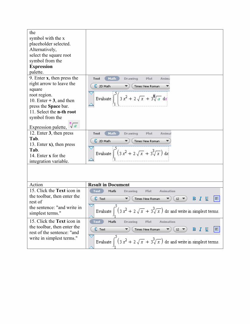
the symbol with the x placeholder selected. Alternatively, select the square root symbol from the Expression palette. 9. Enter x, then press the right arrow to leave the square root region. 10. Enter + 3, and then press the Space bar. 11. Select the n-th root symbol from the
Expression palette,
12. Enter 3, then press Tab. 13. Enter x), then press Tab. 14. Enter x for the integration variable.
Action Result in Document15. Click the Text icon in the toolbar, then enter the rest of the sentence: "and write in simplest terms."
15. Click the Text icon in the toolbar, then enter the rest of the sentence: "and write in simplest terms."
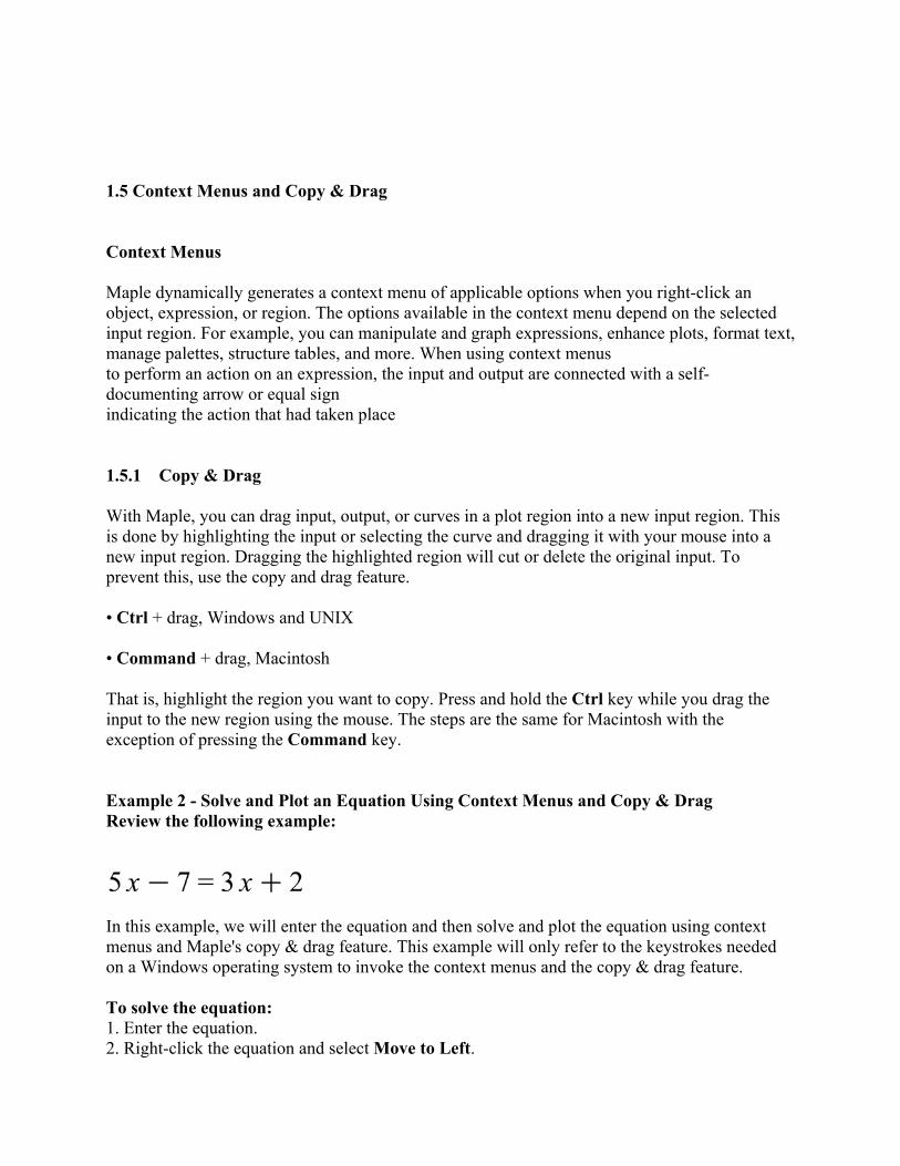
1.5 Context Menus and Copy & Drag
Context Menus Maple dynamically generates a context menu of applicable options when you right-click an object, expression, or region. The options available in the context menu depend on the selected input region. For example, you can manipulate and graph expressions, enhance plots, format text, manage palettes, structure tables, and more. When using context menus to perform an action on an expression, the input and output are connected with a self-documenting arrow or equal sign indicating the action that had taken place 1.5.1 Copy & Drag With Maple, you can drag input, output, or curves in a plot region into a new input region. This is done by highlighting the input or selecting the curve and dragging it with your mouse into a new input region. Dragging the highlighted region will cut or delete the original input. To prevent this, use the copy and drag feature. • Ctrl + drag, Windows and UNIX • Command + drag, Macintosh That is, highlight the region you want to copy. Press and hold the Ctrl key while you drag the input to the new region using the mouse. The steps are the same for Macintosh with the exception of pressing the Command key. Example 2 - Solve and Plot an Equation Using Context Menus and Copy & Drag Review the following example:
In this example, we will enter the equation and then solve and plot the equation using context menus and Maple's copy & drag feature. This example will only refer to the keystrokes needed on a Windows operating system to invoke the context menus and the copy & drag feature. To solve the equation: 1. Enter the equation. 2. Right-click the equation and select Move to Left.
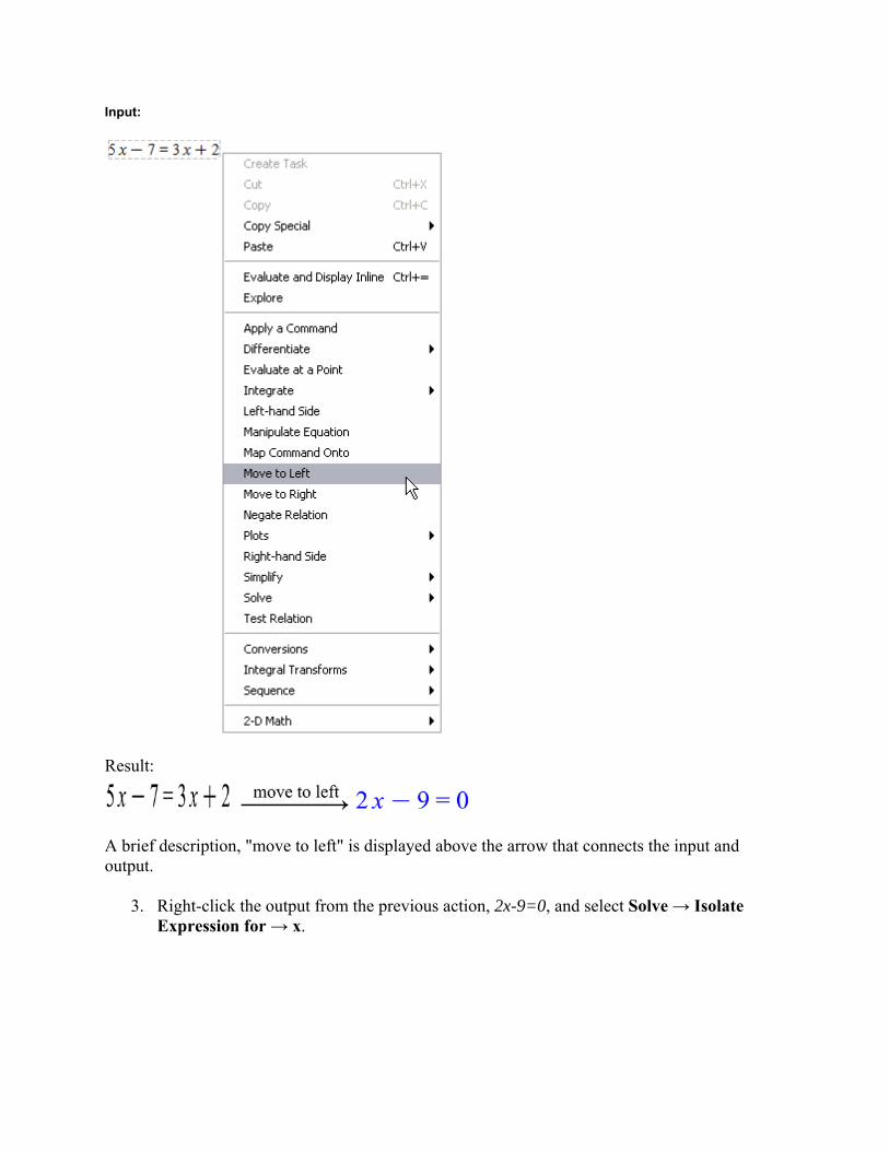
Input:
Result:
A brief description, "move to left" is displayed above the arrow that connects the input and output.
3. Right-click the output from the previous action, 2x-9=0, and select Solve → Isolate Expression for → x.
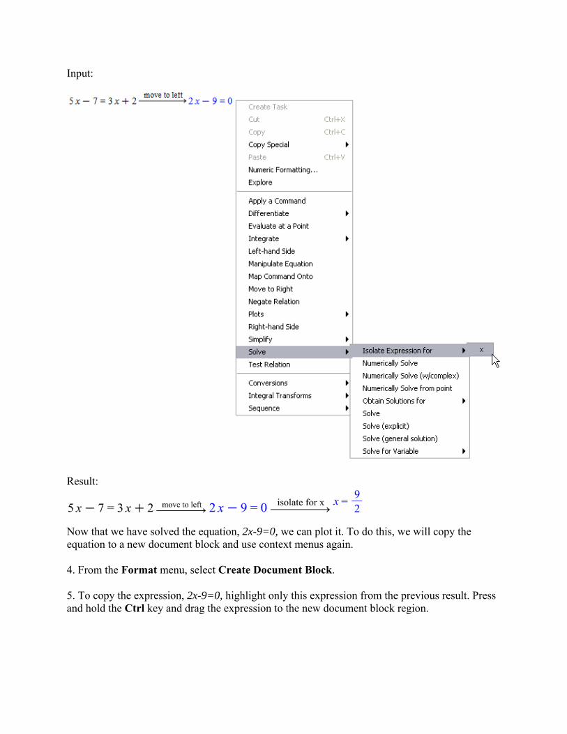
Input:
Result:
Now that we have solved the equation, 2x-9=0, we can plot it. To do this, we will copy the equation to a new document block and use context menus again. 4. From the Format menu, select Create Document Block. 5. To copy the expression, 2x-9=0, highlight only this expression from the previous result. Press and hold the Ctrl key and drag the expression to the new document block region.
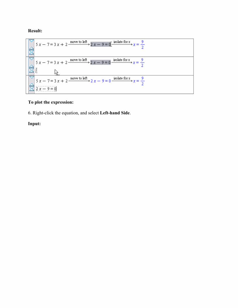
Result:
To plot the expression: 6. Right-click the equation, and select Left-hand Side. Input:
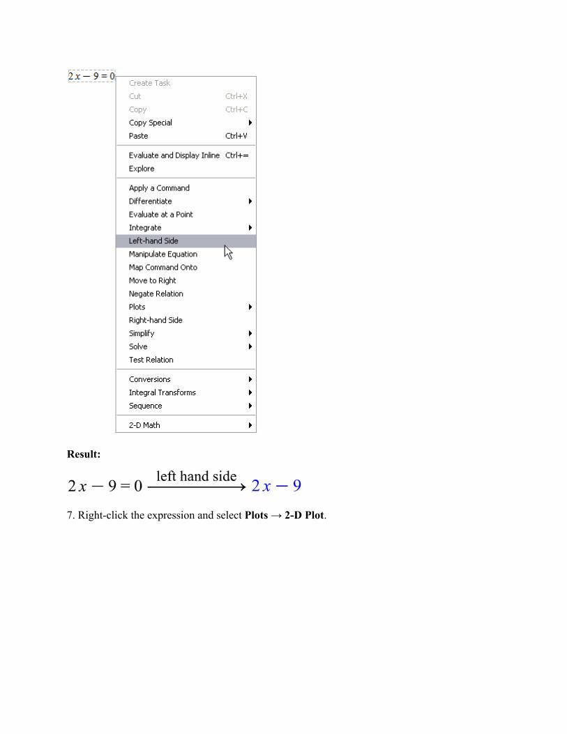
Result:
7. Right-click the expression and select Plots → 2-D Plot.
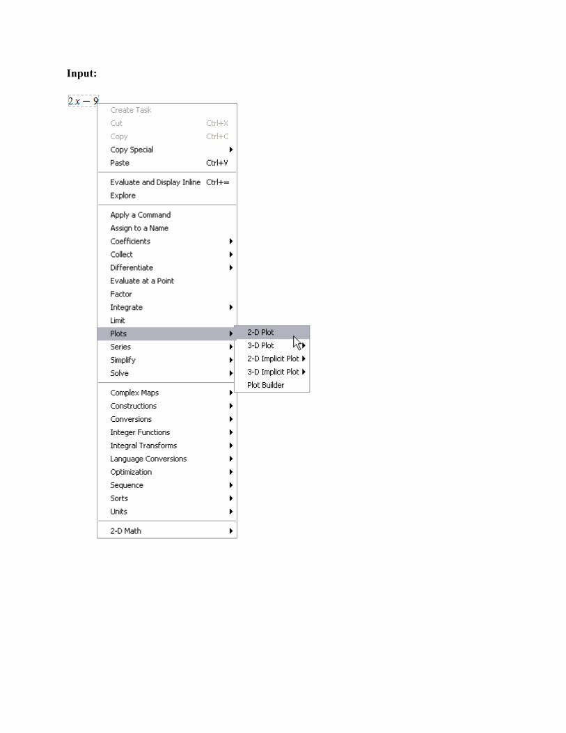
Input:
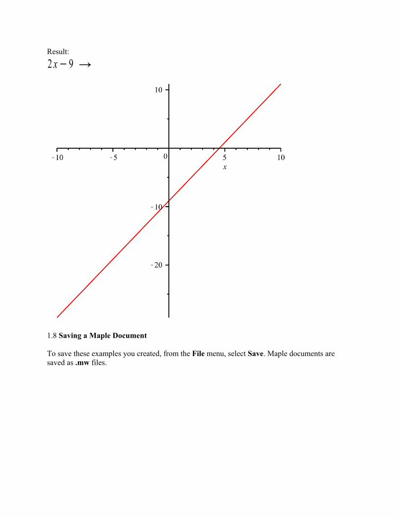
Result:
1.8 Saving a Maple Document To save these examples you created, from the File menu, select Save. Maple documents are saved as .mw files.
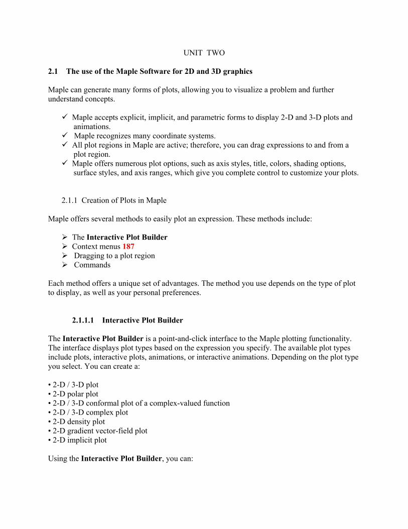
UNIT TWO 2.1 The use of the Maple Software for 2D and 3D graphics
Maple can generate many forms of plots, allowing you to visualize a problem and further understand concepts. Maple accepts explicit, implicit, and parametric forms to display 2-D and 3-D plots and
animations. Maple recognizes many coordinate systems. All plot regions in Maple are active; therefore, you can drag expressions to and from a
plot region. Maple offers numerous plot options, such as axis styles, title, colors, shading options,
surface styles, and axis ranges, which give you complete control to customize your plots.
2.1.1 Creation of Plots in Maple
Maple offers several methods to easily plot an expression. These methods include: The Interactive Plot Builder Context menus 187 Dragging to a plot region Commands
Each method offers a unique set of advantages. The method you use depends on the type of plot to display, as well as your personal preferences.
2.1.1.1 Interactive Plot Builder The Interactive Plot Builder is a point-and-click interface to the Maple plotting functionality. The interface displays plot types based on the expression you specify. The available plot types include plots, interactive plots, animations, or interactive animations. Depending on the plot type you select. You can create a: • 2-D / 3-D plot • 2-D polar plot • 2-D / 3-D conformal plot of a complex-valued function • 2-D / 3-D complex plot • 2-D density plot • 2-D gradient vector-field plot • 2-D implicit plot Using the Interactive Plot Builder, you can:
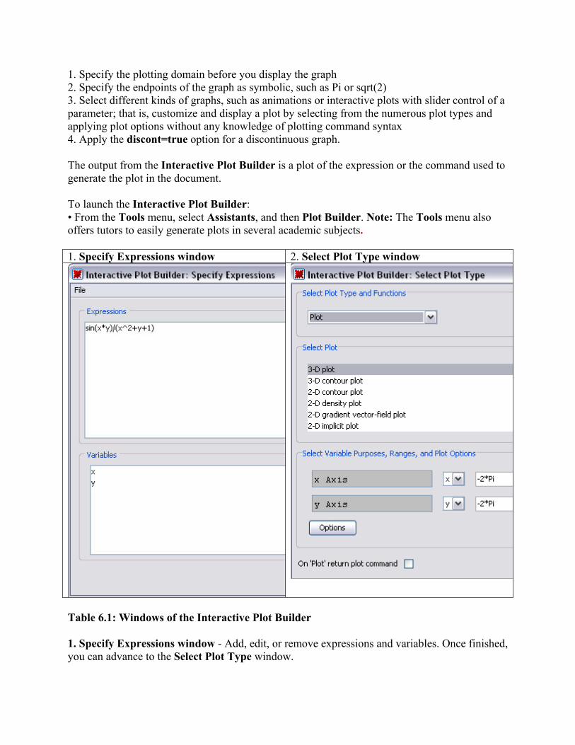
1. Specify the plotting domain before you display the graph 2. Specify the endpoints of the graph as symbolic, such as Pi or sqrt(2) 3. Select different kinds of graphs, such as animations or interactive plots with slider control of a parameter; that is, customize and display a plot by selecting from the numerous plot types and applying plot options without any knowledge of plotting command syntax 4. Apply the discont=true option for a discontinuous graph. The output from the Interactive Plot Builder is a plot of the expression or the command used to generate the plot in the document. To launch the Interactive Plot Builder: • From the Tools menu, select Assistants, and then Plot Builder. Note: The Tools menu also offers tutors to easily generate plots in several academic subjects. 1. Specify Expressions window 2. Select Plot Type window
Table 6.1: Windows of the Interactive Plot Builder 1. Specify Expressions window - Add, edit, or remove expressions and variables. Once finished, you can advance to the Select Plot Type window.
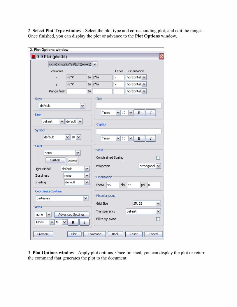
2. Select Plot Type window - Select the plot type and corresponding plot, and edit the ranges. Once finished, you can display the plot or advance to the Plot Options window.
3. Plot Options window
3. Plot Options window - Apply plot options. Once finished, you can display the plot or return the command that generates the plot to the document.
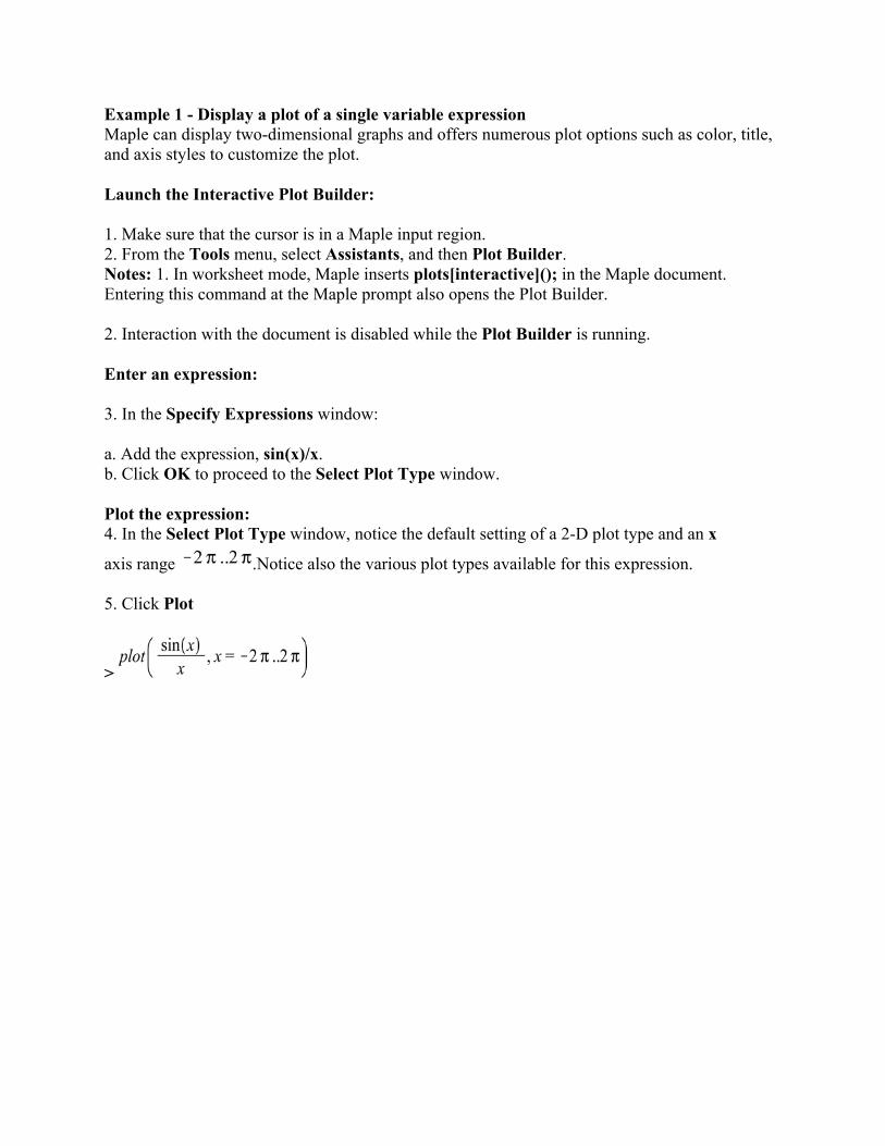
Example 1 - Display a plot of a single variable expression Maple can display two-dimensional graphs and offers numerous plot options such as color, title, and axis styles to customize the plot. Launch the Interactive Plot Builder: 1. Make sure that the cursor is in a Maple input region. 2. From the Tools menu, select Assistants, and then Plot Builder. Notes: 1. In worksheet mode, Maple inserts plots[interactive](); in the Maple document. Entering this command at the Maple prompt also opens the Plot Builder. 2. Interaction with the document is disabled while the Plot Builder is running. Enter an expression: 3. In the Specify Expressions window: a. Add the expression, sin(x)/x. b. Click OK to proceed to the Select Plot Type window. Plot the expression: 4. In the Select Plot Type window, notice the default setting of a 2-D plot type and an x
axis range .Notice also the various plot types available for this expression. 5. Click Plot
>
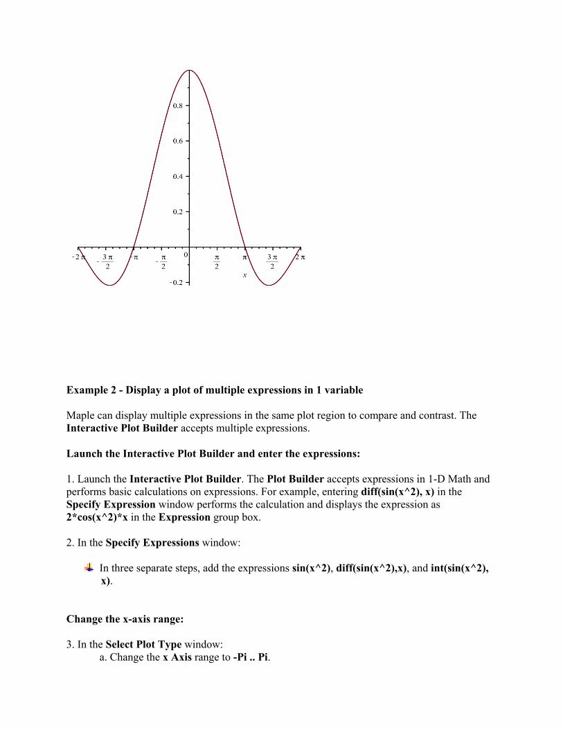
Example 2 - Display a plot of multiple expressions in 1 variable Maple can display multiple expressions in the same plot region to compare and contrast. The Interactive Plot Builder accepts multiple expressions. Launch the Interactive Plot Builder and enter the expressions: 1. Launch the Interactive Plot Builder. The Plot Builder accepts expressions in 1-D Math and performs basic calculations on expressions. For example, entering diff(sin(x^2), x) in the Specify Expression window performs the calculation and displays the expression as 2*cos(x^2)*x in the Expression group box. 2. In the Specify Expressions window:
In three separate steps, add the expressions sin(x^2), diff(sin(x^2),x), and int(sin(x^2), x).
Change the x-axis range: 3. In the Select Plot Type window:
a. Change the x Axis range to -Pi .. Pi.
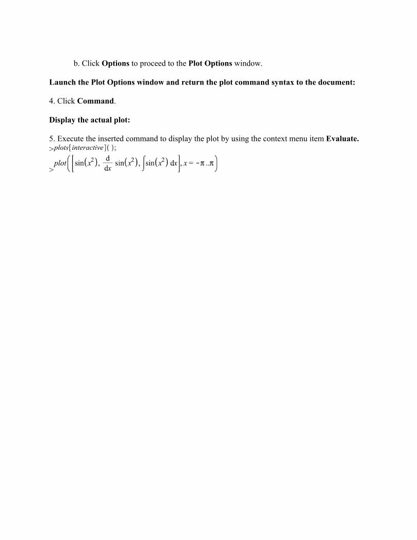
b. Click Options to proceed to the Plot Options window.
Launch the Plot Options window and return the plot command syntax to the document: 4. Click Command. Display the actual plot: 5. Execute the inserted command to display the plot by using the context menu item Evaluate. >
>
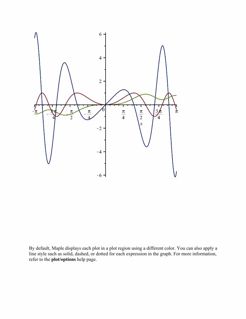
By default, Maple displays each plot in a plot region using a different color. You can also apply a line style such as solid, dashed, or dotted for each expression in the graph. For more information, refer to the plot/options help page.

Example 3 - Display a plot of a multi-variate expression Maple can display three-dimensional plots and offers numerous plot options such as light models, surface styles, and shadings to allow you to customize the plot. Launch the Interactive Plot Builder and enter an expression: 1. Add the expression (1+sin(x*y))/(x^2+y^2). In the Select Plot Type window: 2. Notice the available plot types for an expression with 2 variables, as well as the plot objects for each type. 3. Click Options. In the Plot Options window: 4. From the Variables column at the top of the dialog, change the Range from field to 0 .. 0.05. 5. From the Label column, enter z. 6. From the Style group box, select surface. 7. From the Color group box, in the Light Model drop-down menu, select green-red. 8. From the Color group box, in the Shading, drop-down menu, select z (grayscale). 9. From the Miscellaneous group box, in the Grid Size drop-down menu, select 40, 40. Plot the expression: 10. Click Plot.
>
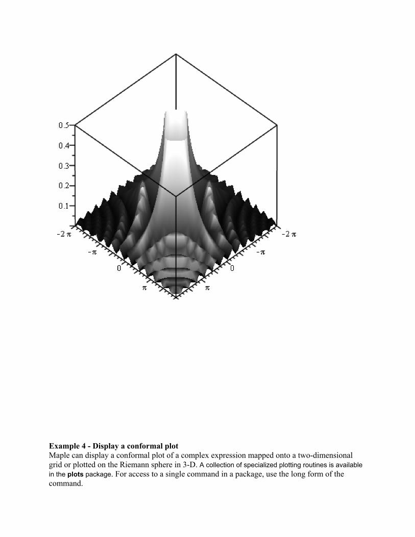
Example 4 - Display a conformal plot Maple can display a conformal plot of a complex expression mapped onto a two-dimensional grid or plotted on the Riemann sphere in 3-D. A collection of specialized plotting routines is available in the plots package. For access to a single command in a package, use the long form of the command.

Launch the Interactive Plot Builder and enter an expression: 1. Add the expression z^3. In the Select Plot Type window: 2. From the Select Plot group box, select 2-D conformal plot of a complex-valued function. 3. Change the range of the z parameter to 0 .. 2+2*I. In the Plot Options window: 4. From the Axes group box, select normal. 5. From the Miscellaneous group box, select the Grid Size drop-down menu option 20, 20. Plot the expression: 6. Click Plot.
>
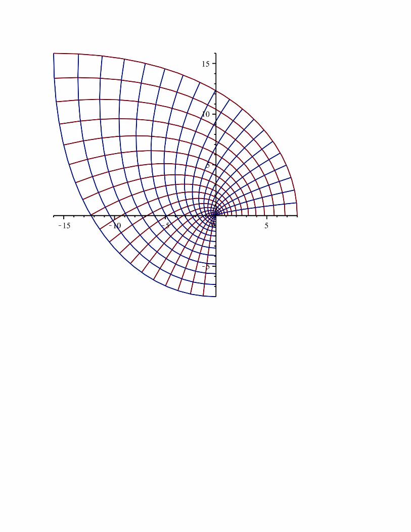
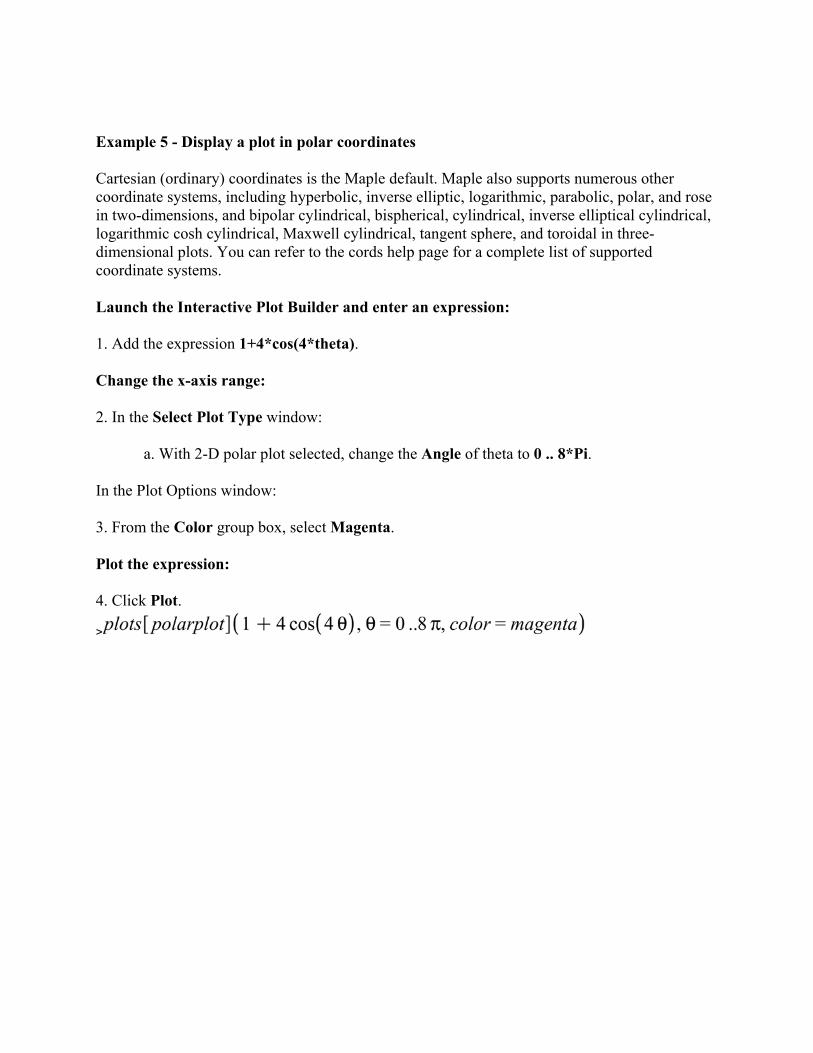
Example 5 - Display a plot in polar coordinates Cartesian (ordinary) coordinates is the Maple default. Maple also supports numerous other coordinate systems, including hyperbolic, inverse elliptic, logarithmic, parabolic, polar, and rose in two-dimensions, and bipolar cylindrical, bispherical, cylindrical, inverse elliptical cylindrical, logarithmic cosh cylindrical, Maxwell cylindrical, tangent sphere, and toroidal in three-dimensional plots. You can refer to the cords help page for a complete list of supported coordinate systems. Launch the Interactive Plot Builder and enter an expression: 1. Add the expression 1+4*cos(4*theta). Change the x-axis range: 2. In the Select Plot Type window:
a. With 2-D polar plot selected, change the Angle of theta to 0 .. 8*Pi. In the Plot Options window: 3. From the Color group box, select Magenta. Plot the expression: 4. Click Plot.
>
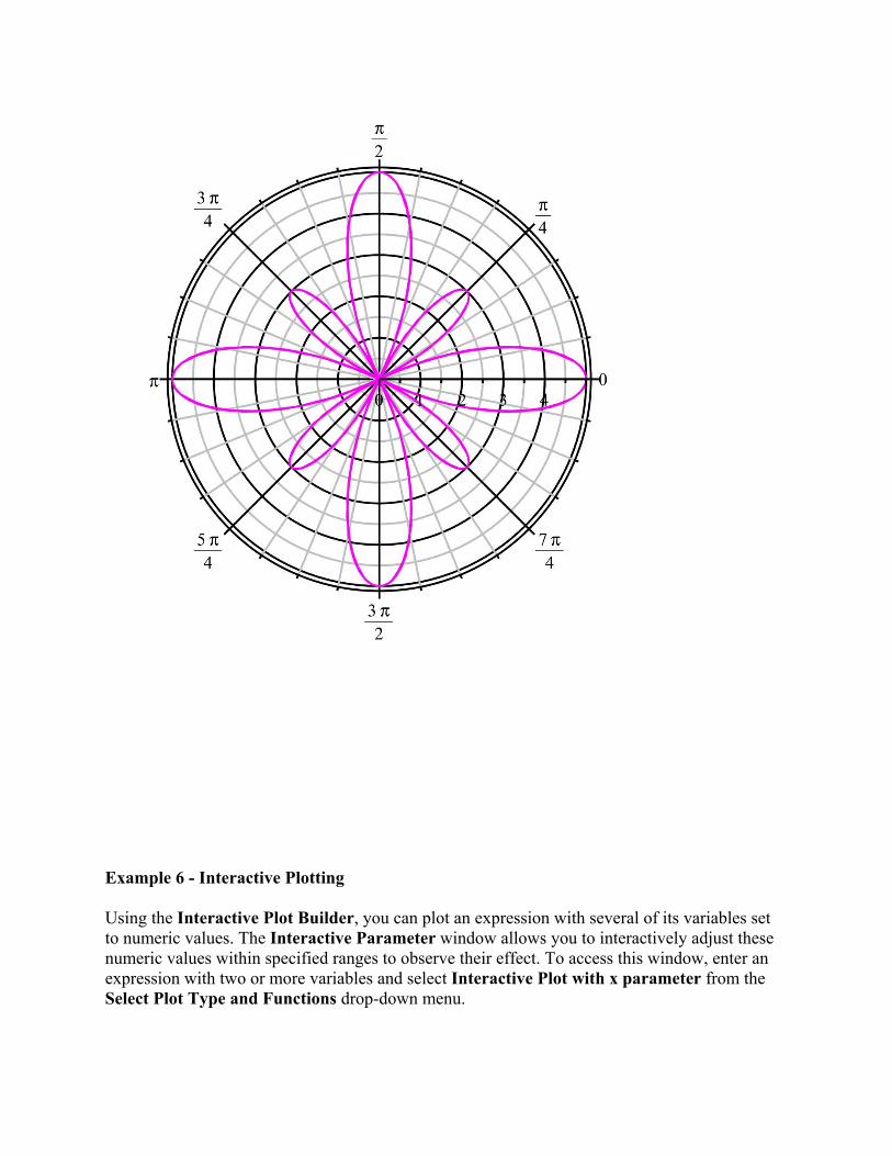
Example 6 - Interactive Plotting Using the Interactive Plot Builder, you can plot an expression with several of its variables set to numeric values. The Interactive Parameter window allows you to interactively adjust these numeric values within specified ranges to observe their effect. To access this window, enter an expression with two or more variables and select Interactive Plot with x parameter from the Select Plot Type and Functions drop-down menu.
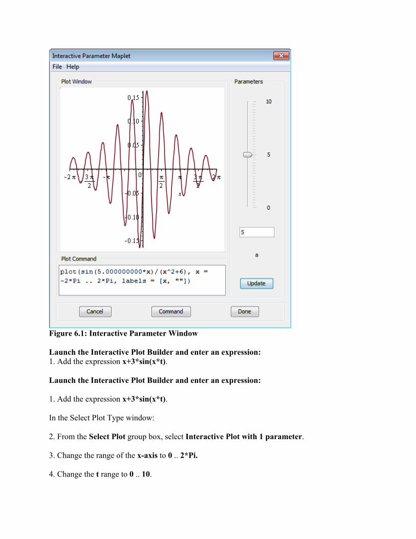
Figure 6.1: Interactive Parameter Window Launch the Interactive Plot Builder and enter an expression: 1. Add the expression x+3*sin(x*t). Launch the Interactive Plot Builder and enter an expression: 1. Add the expression x+3*sin(x*t). In the Select Plot Type window: 2. From the Select Plot group box, select Interactive Plot with 1 parameter. 3. Change the range of the x-axis to 0 .. 2*Pi. 4. Change the t range to 0 .. 10.
5. Click Plot to open the Interactive Parameter window. Note: To apply plot options before interactively adjusting the plot, click Options to open the Plot Options window. After setting the plot options, click Plot to display the Interactive Parameter window. 6. To adjust the numeric values, use the slider. 7. Click Done to place the plot in the Maple document. The plot and plot3d Commands The final method for creating plots is entering plotting commands. The main advantages of using plotting commands are the availability of all Maple plot structures and the greater control over the plot output.
plot(plotexpression, x=a..b, ...) plot3d(plotexpression, x=a..b, y=a..b, ...) • plotexpression - expression to be plotted • x=a..b - name and horizontal range • y=a..b - name and vertical range
UNIT TWO
2.0 Introduction to the Finance Package The Finance package assists you in performing financial calculations. With it, you can calculate the present value and the accumulated value of annuities, growing annuities, perpetuities, growing perpetuities and level coupon bonds. Moreover, it can also help you compute the yield to maturity of a bond. You can construct an amortization table, determine the effective rate of interest for a given compound interest rate, and find the present value and the future value of a fixed quantity for a given compound interest rate.
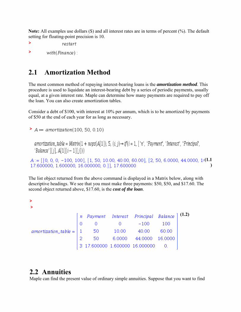
Note: All examples use dollars ($) and all interest rates are in terms of percent (%). The default setting for floating-point precision is 10. >
>
2.1 Amortization Method
The most common method of repaying interest-bearing loans is the amortization method. This procedure is used to liquidate an interest-bearing debt by a series of periodic payments, usually equal, at a given interest rate. Maple can determine how many payments are required to pay off the loan. You can also create amortization tables. Consider a debt of $100, with interest at 10% per annum, which is to be amortized by payments of $50 at the end of each year for as long as necessary. >
(1.1)
The list object returned from the above command is displayed in a Matrix below, along with descriptive headings. We see that you must make three payments: $50, $50, and $17.60. The second object returned above, $17.60, is the cost of the loan. > >
(1.2)
2.2 Annuities Maple can find the present value of ordinary simple annuities. Suppose that you want to find
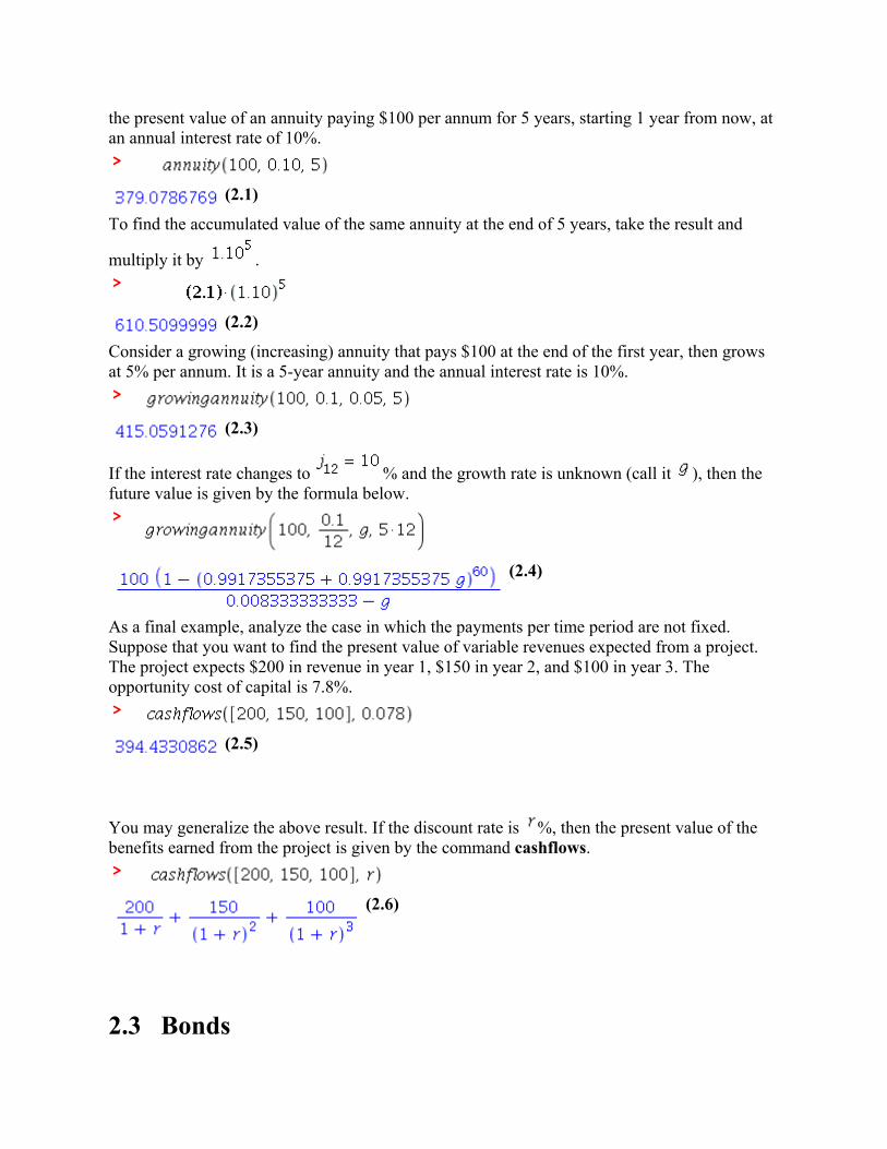
the present value of an annuity paying $100 per annum for 5 years, starting 1 year from now, at an annual interest rate of 10%. >
(2.1)
To find the accumulated value of the same annuity at the end of 5 years, take the result and
multiply it by . >
(2.2)
Consider a growing (increasing) annuity that pays $100 at the end of the first year, then grows at 5% per annum. It is a 5-year annuity and the annual interest rate is 10%. >
(2.3)
If the interest rate changes to % and the growth rate is unknown (call it ), then the future value is given by the formula below. >
(2.4)
As a final example, analyze the case in which the payments per time period are not fixed. Suppose that you want to find the present value of variable revenues expected from a project. The project expects $200 in revenue in year 1, $150 in year 2, and $100 in year 3. The opportunity cost of capital is 7.8%. >
(2.5)
You may generalize the above result. If the discount rate is %, then the present value of the benefits earned from the project is given by the command cashflows. >
(2.6)
2.3 Bonds
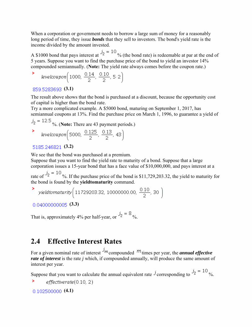
When a corporation or government needs to borrow a large sum of money for a reasonably long period of time, they issue bonds that they sell to investors. The bond's yield rate is the income divided by the amount invested.
A $1000 bond that pays interest at % (the bond rate) is redeemable at par at the end of 5 years. Suppose you want to find the purchase price of the bond to yield an investor 14% compounded semiannually. (Note: The yield rate always comes before the coupon rate.) >
(3.1)
The result above shows that the bond is purchased at a discount, because the opportunity cost of capital is higher than the bond rate. Try a more complicated example. A $5000 bond, maturing on September 1, 2017, has semiannual coupons at 13%. Find the purchase price on March 1, 1996, to guarantee a yield of
%. (Note: There are 43 payment periods.) >
(3.2)
We see that the bond was purchased at a premium. Suppose that you want to find the yield rate to maturity of a bond. Suppose that a large corporation issues a 15-year bond that has a face value of $10,000,000, and pays interest at a
rate of %. If the purchase price of the bond is $11,729,203.32, the yield to maturity for the bond is found by the yieldtomaturity command. >
(3.3)
That is, approximately 4% per half-year, or %. 2.4 Effective Interest Rates
For a given nominal rate of interest compounded times per year, the annual effective rate of interest is the rate j which, if compounded annually, will produce the same amount of interest per year.
Suppose that you want to calculate the annual equivalent rate corresponding to %. >
(4.1)
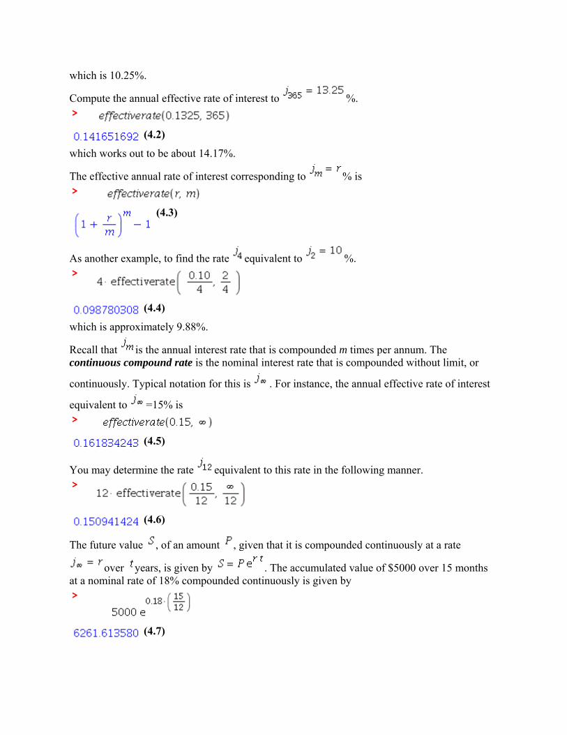
which is 10.25%.
Compute the annual effective rate of interest to %. >
(4.2)
which works out to be about 14.17%.
The effective annual rate of interest corresponding to % is >
(4.3)
As another example, to find the rate equivalent to %. >
(4.4)
which is approximately 9.88%.
Recall that is the annual interest rate that is compounded m times per annum. The continuous compound rate is the nominal interest rate that is compounded without limit, or
continuously. Typical notation for this is . For instance, the annual effective rate of interest
equivalent to =15% is >
(4.5)
You may determine the rate equivalent to this rate in the following manner. >
(4.6)
The future value , of an amount , given that it is compounded continuously at a rate
over years, is given by . The accumulated value of $5000 over 15 months at a nominal rate of 18% compounded continuously is given by >
(4.7)
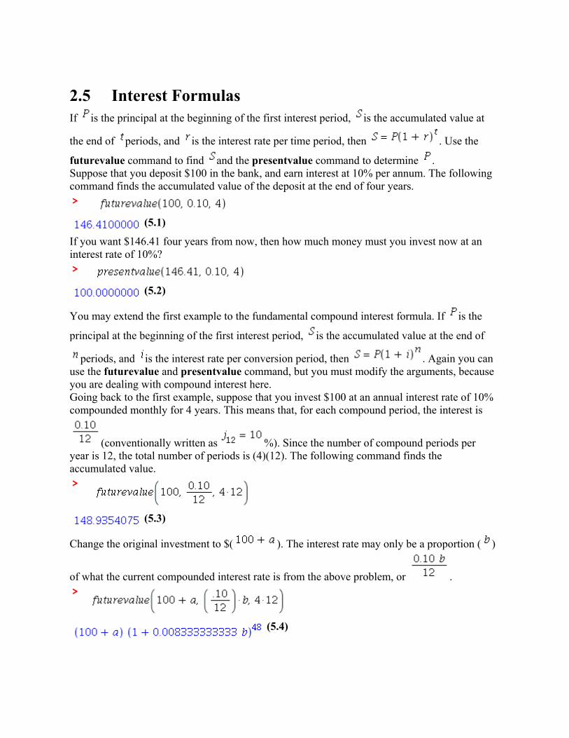
2.5 Interest Formulas
If is the principal at the beginning of the first interest period, is the accumulated value at
the end of periods, and is the interest rate per time period, then . Use the
futurevalue command to find and the presentvalue command to determine . Suppose that you deposit $100 in the bank, and earn interest at 10% per annum. The following command finds the accumulated value of the deposit at the end of four years. >
(5.1)
If you want $146.41 four years from now, then how much money must you invest now at an interest rate of 10%? >
(5.2)
You may extend the first example to the fundamental compound interest formula. If is the
principal at the beginning of the first interest period, is the accumulated value at the end of
periods, and is the interest rate per conversion period, then . Again you can use the futurevalue and presentvalue command, but you must modify the arguments, because you are dealing with compound interest here. Going back to the first example, suppose that you invest $100 at an annual interest rate of 10% compounded monthly for 4 years. This means that, for each compound period, the interest is
(conventionally written as %). Since the number of compound periods per year is 12, the total number of periods is (4)(12). The following command finds the accumulated value. >
(5.3)
Change the original investment to $( ). The interest rate may only be a proportion ( )
of what the current compounded interest rate is from the above problem, or . >
(5.4)
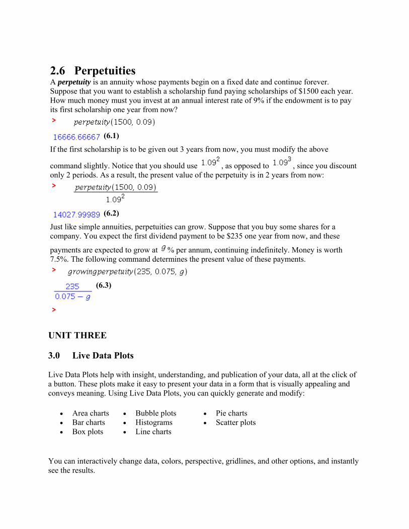
2.6 Perpetuities
A perpetuity is an annuity whose payments begin on a fixed date and continue forever. Suppose that you want to establish a scholarship fund paying scholarships of $1500 each year. How much money must you invest at an annual interest rate of 9% if the endowment is to pay its first scholarship one year from now? >
(6.1)
If the first scholarship is to be given out 3 years from now, you must modify the above
command slightly. Notice that you should use , as opposed to , since you discount only 2 periods. As a result, the present value of the perpetuity is in 2 years from now: >
(6.2)
Just like simple annuities, perpetuities can grow. Suppose that you buy some shares for a company. You expect the first dividend payment to be $235 one year from now, and these
payments are expected to grow at % per annum, continuing indefinitely. Money is worth 7.5%. The following command determines the present value of these payments. >
(6.3)
>
UNIT THREE
3.0 Live Data Plots
Live Data Plots help with insight, understanding, and publication of your data, all at the click of a button. These plots make it easy to present your data in a form that is visually appealing and conveys meaning. Using Live Data Plots, you can quickly generate and modify:
Area charts Bar charts Box plots
Bubble plots Histograms Line charts
Pie charts Scatter plots
You can interactively change data, colors, perspective, gridlines, and other options, and instantly see the results.
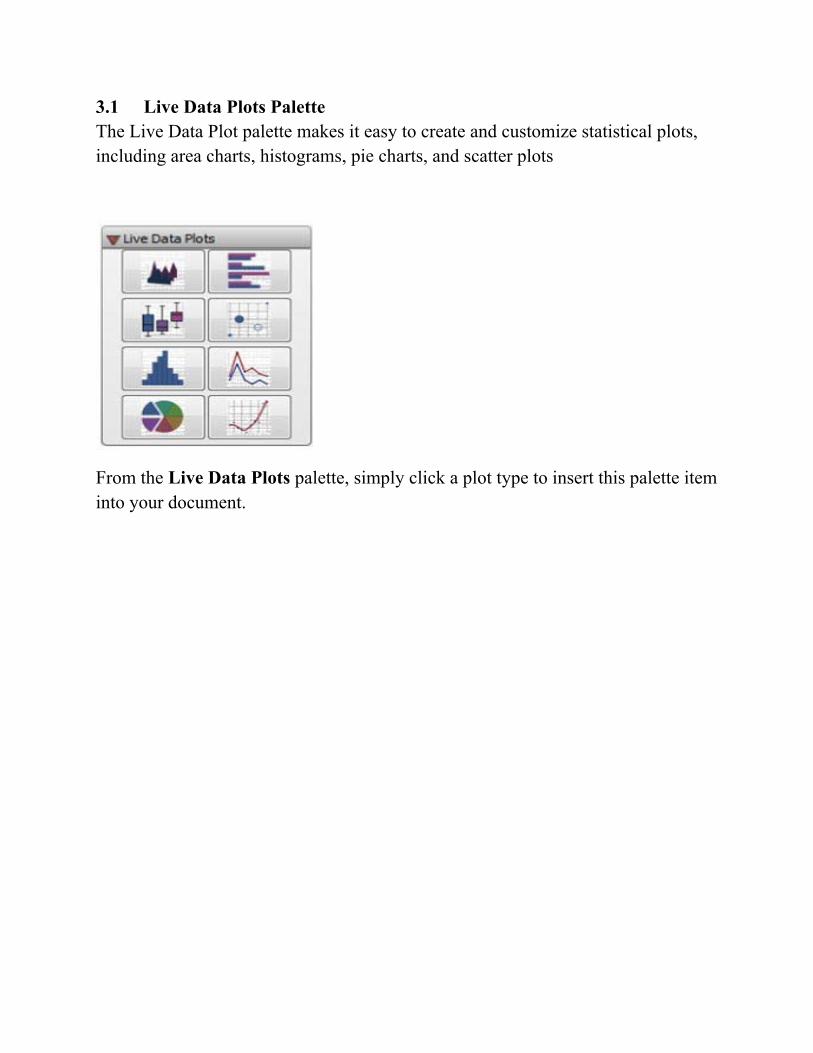
3.1 Live Data Plots Palette The Live Data Plot palette makes it easy to create and customize statistical plots, including area charts, histograms, pie charts, and scatter plots
From the Live Data Plots palette, simply click a plot type to insert this palette item into your document.
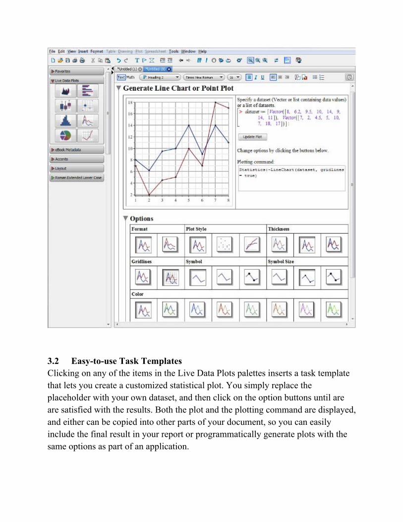
3.2 Easy-to-use Task Templates Clicking on any of the items in the Live Data Plots palettes inserts a task template that lets you create a customized statistical plot. You simply replace the placeholder with your own dataset, and then click on the option buttons until are are satisfied with the results. Both the plot and the plotting command are displayed, and either can be copied into other parts of your document, so you can easily include the final result in your report or programmatically generate plots with the same options as part of an application.
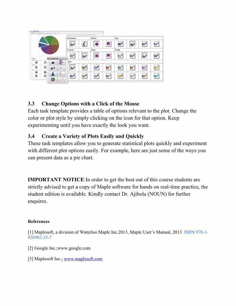
3.3 Change Options with a Click of the Mouse Each task template provides a table of options relevant to the plot. Change the color or plot style by simply clicking on the icon for that option. Keep experimenting until you have exactly the look you want.
3.4 Create a Variety of Plots Easily and Quickly These task templates allow you to generate statistical plots quickly and experiment with different plot options easily. For example, here are just some of the ways you can present data as a pie chart.
IMPORTANT NOTICE:In order to get the best out of this course students are strictly advised to get a copy of Maple software for hands on real-time practice, the student edition is available. Kindly contact Dr. Ajibola (NOUN) for further enquires.
References [1] Maplesoft, a division of Waterloo Maple Inc.2013, Maple User’s Manual, 2013. ISBN 978-1-926902-35-7 [2] Google Inc.;www.google.com [3] Maplesoft Inc.; www.maplesoft.com
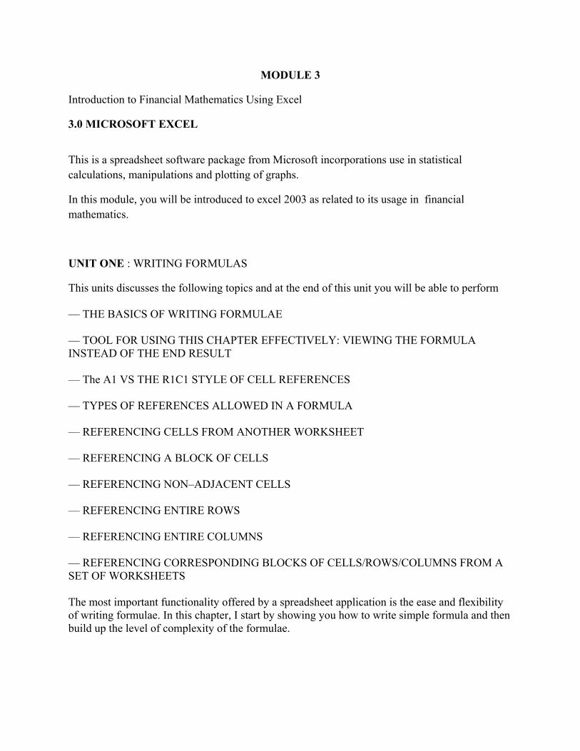
MODULE 3
Introduction to Financial Mathematics Using Excel
3.0 MICROSOFT EXCEL
This is a spreadsheet software package from Microsoft incorporations use in statistical calculations, manipulations and plotting of graphs.
In this module, you will be introduced to excel 2003 as related to its usage in financial mathematics.
UNIT ONE : WRITING FORMULAS
This units discusses the following topics and at the end of this unit you will be able to perform — THE BASICS OF WRITING FORMULAE — TOOL FOR USING THIS CHAPTER EFFECTIVELY: VIEWING THE FORMULA INSTEAD OF THE END RESULT — The A1 VS THE R1C1 STYLE OF CELL REFERENCES — TYPES OF REFERENCES ALLOWED IN A FORMULA — REFERENCING CELLS FROM ANOTHER WORKSHEET — REFERENCING A BLOCK OF CELLS — REFERENCING NON–ADJACENT CELLS — REFERENCING ENTIRE ROWS — REFERENCING ENTIRE COLUMNS — REFERENCING CORRESPONDING BLOCKS OF CELLS/ROWS/COLUMNS FROM A SET OF WORKSHEETS The most important functionality offered by a spreadsheet application is the ease and flexibility of writing formulae. In this chapter, I start by showing you how to write simple formula and then build up the level of complexity of the formulae.
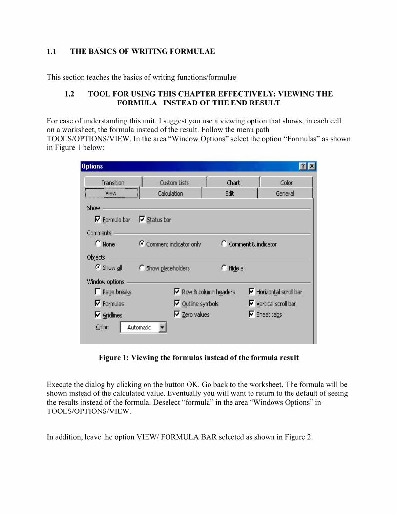
1.1 THE BASICS OF WRITING FORMULAE
This section teaches the basics of writing functions/formulae
1.2 TOOL FOR USING THIS CHAPTER EFFECTIVELY: VIEWING THE FORMULA INSTEAD OF THE END RESULT
For ease of understanding this unit, I suggest you use a viewing option that shows, in each cell on a worksheet, the formula instead of the result. Follow the menu path TOOLS/OPTIONS/VIEW. In the area “Window Options” select the option “Formulas” as shown in Figure 1 below:
Figure 1: Viewing the formulas instead of the formula result Execute the dialog by clicking on the button OK. Go back to the worksheet. The formula will be shown instead of the calculated value. Eventually you will want to return to the default of seeing the results instead of the formula. Deselect “formula” in the area “Windows Options” in TOOLS/OPTIONS/VIEW.
In addition, leave the option VIEW/ FORMULA BAR selected as shown in Figure 2.
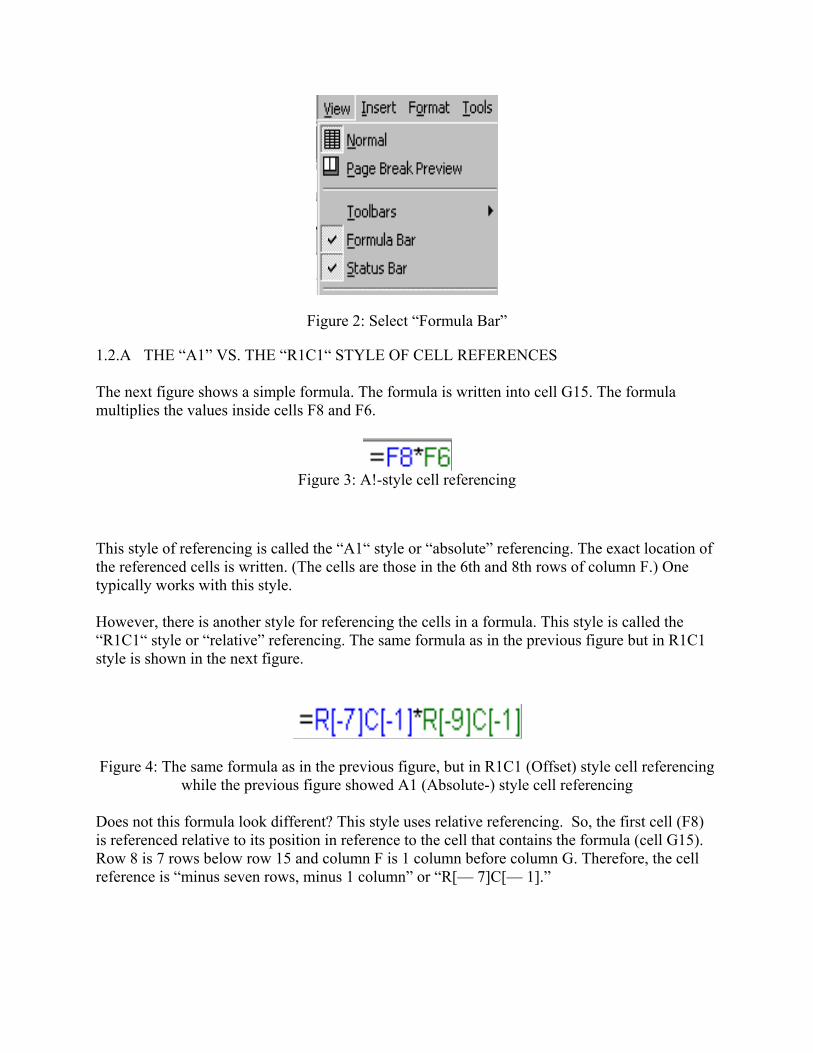
Figure 2: Select “Formula Bar”
1.2.A THE “A1” VS. THE “R1C1“ STYLE OF CELL REFERENCES The next figure shows a simple formula. The formula is written into cell G15. The formula multiplies the values inside cells F8 and F6.
Figure 3: A!-style cell referencing
This style of referencing is called the “A1“ style or “absolute” referencing. The exact location of the referenced cells is written. (The cells are those in the 6th and 8th rows of column F.) One typically works with this style. However, there is another style for referencing the cells in a formula. This style is called the “R1C1“ style or “relative” referencing. The same formula as in the previous figure but in R1C1 style is shown in the next figure.
Figure 4: The same formula as in the previous figure, but in R1C1 (Offset) style cell referencing while the previous figure showed A1 (Absolute-) style cell referencing
Does not this formula look different? This style uses relative referencing. So, the first cell (F8) is referenced relative to its position in reference to the cell that contains the formula (cell G15). Row 8 is 7 rows below row 15 and column F is 1 column before column G. Therefore, the cell reference is “minus seven rows, minus 1 column” or “R[— 7]C[— 1].”
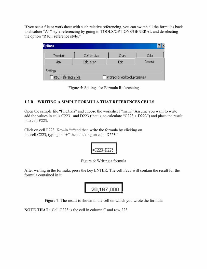
If you see a file or worksheet with such relative referencing, you can switch all the formulas back to absolute “A1” style referencing by going to TOOLS/OPTIONS/GENERAL and deselecting the option “R1C1 reference style.”
Figure 5: Settings for Formula Referencing
1.2.B WRITING A SIMPLE FORMULA THAT REFERENCES CELLS Open the sample file “File3.xls” and choose the worksheet “main.” Assume you want to write add the values in cells C2231 and D223 (that is, to calculate “C223 + D223”) and place the result into cell F223. Click on cell F223. Key-in “=“and then write the formula by clicking on the cell C223, typing in “+” then clicking on cell “D223.”
Figure 6: Writing a formula
After writing in the formula, press the key ENTER. The cell F223 will contain the result for the formula contained in it.
Figure 7: The result is shown in the cell on which you wrote the formula
NOTE THAT: Cell C223 is the cell in column C and row 223.
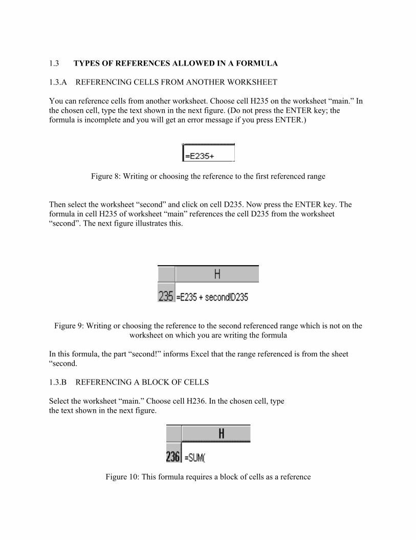
1.3 TYPES OF REFERENCES ALLOWED IN A FORMULA 1.3.A REFERENCING CELLS FROM ANOTHER WORKSHEET You can reference cells from another worksheet. Choose cell H235 on the worksheet “main.” In the chosen cell, type the text shown in the next figure. (Do not press the ENTER key; the formula is incomplete and you will get an error message if you press ENTER.)
Figure 8: Writing or choosing the reference to the first referenced range
Then select the worksheet “second” and click on cell D235. Now press the ENTER key. The formula in cell H235 of worksheet “main” references the cell D235 from the worksheet “second”. The next figure illustrates this.
Figure 9: Writing or choosing the reference to the second referenced range which is not on the worksheet on which you are writing the formula
In this formula, the part “second!” informs Excel that the range referenced is from the sheet “second. 1.3.B REFERENCING A BLOCK OF CELLS Select the worksheet “main.” Choose cell H236. In the chosen cell, type the text shown in the next figure.
Figure 10: This formula requires a block of cells as a reference
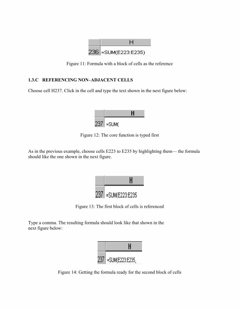
Figure 11: Formula with a block of cells as the reference
1.3.C REFERENCING NON–ADJACENT CELLS Choose cell H237. Click in the cell and type the text shown in the next figure below:
Figure 12: The core function is typed first
As in the previous example, choose cells E223 to E235 by highlighting them— the formula should like the one shown in the next figure.
Figure 13: The first block of cells is referenced
Type a comma. The resulting formula should look like that shown in the next figure below:
Figure 14: Getting the formula ready for the second block of cells
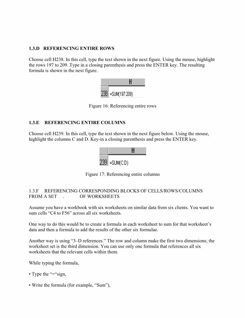
1.3.D REFERENCING ENTIRE ROWS Choose cell H238. In this cell, type the text shown in the next figure. Using the mouse, highlight the rows 197 to 209. Type in a closing parenthesis and press the ENTER key. The resulting formula is shown in the next figure.
Figure 16: Referencing entire rows
1.3.E REFERENCING ENTIRE COLUMNS Choose cell H239. In this cell, type the text shown in the next figure below. Using the mouse, highlight the columns C and D. Key-in a closing parenthesis and press the ENTER key.
Figure 17: Referencing entire columns
1.3.F REFERENCING CORRESPONDING BLOCKS OF CELLS/ROWS/COLUMNS FROM A SET . OF WORKSHEETS Assume you have a workbook with six worksheets on similar data from six clients. You want to sum cells “C4 to F56” across all six worksheets. One way to do this would be to create a formula in each worksheet to sum for that worksheet’s data and then a formula to add the results of the other six formulae. Another way is using “3–D references.” The row and column make the first two dimensions; the worksheet set is the third dimension. You can use only one formula that references all six worksheets that the relevant cells within them. While typing the formula, • Type the “=“sign, • Write the formula (for example, “Sum”),
• Place an opening parenthesis “(,” then • Select the six worksheets by clicking at the name tab of the first one and then pressing down SHIFT and clicking on the name tab of the sixth worksheet, and then • Highlight the relevant cell range on any one of them, • Type in the closing parenthesis “)” • And press the ENTER key to get the formula
1.4 WORKING SIMULTANEOUSLY ON CELLS IN DIFFERENT WORKSHEETS Assume your workbook has 18 worksheets, each for a different country. Assume further that all the worksheets have a similar composition— the same variables in the same columns and rows. You want to make some calculations for each country/worksheet. The long way of doing this is calculating separately for each country/worksheet. However, this means that you will be repeating the same step 17 times. An easier way is to select all the worksheets and do the calculations only once. Whenever you select several worksheets2 and perform some formatting on a range of cells, rows, or columns in one of the worksheets, the same is automatically conducted for the same range of cells, rows, or columns in all the selected worksheets. If you write a formula on a cell (for example, in cell “C3”) in one of the worksheets, the same formula is automatically written in the same cell (in cell “C3”) on all the selected worksheets. Whenever you copy and paste formulas or cell values in one worksheet, the same copy and paste action is replicated on the other worksheets. Note that : Selecting multiple consecutive worksheets: (a) click on the first sheet, (b) press down on the SHIFT key, and, (c) click on the last sheet. Selecting multiple nonconsecutive worksheets: (a) click on the first sheet, (b) press down on the CTRL key, and, (c) one by one, click on the other worksheets you want to select. If a sheet is selected successfully, its sheet tab will be highlighted.
Once again, in order to facilitate your understanding of this topic, the feature is best learned by practice. So, try it out using your own sample file named file1.xls
=SUM(Sheet1:Sheet6!’’C4:F56’’)

“Files1.xls.” In that file, all the worksheets whose names are country names (see the worksheets “Algeria,” “Bahrain,” … , “Yemen”) are identical in their structure. — In cell D5 of each cell, I wanted the formula “= (C5/C4) — 1.” I selected all the worksheets and typed the formula into cell D5 of only one of the worksheets. The formula was automatically replicated on all the worksheets I had selected. — Write the formula “= (C6/C5) — 1” into cell D6 of all these worksheets using this method. With all the worksheets selected, try different things like formatting cells, changing the width of columns, etc. Notice that you only have to work on one worksheet, and the work is automatically replicated for all the selected worksheets. The use of this feature is optimized if data in separate worksheets is arranged in a manner that facilitates work on several sheets. UNIT 2 COPYING/CUTTING AND PASTING FORMULAE This unit will teach the following topics: — COPYING AND PASTING A FORMULA TO OTHER CELLS IN THE SAME COLUMN — COPYING AND PASTING A FORMULA TO OTHER CELLS IN THE SAME ROW — COPYING AND PASTING A FORMULA TO OTHER CELLS IN A DIFFERENT ROW AND COLUMN — CONTROLLING CELL REFERENCE BEHAVIOR WHEN COPYING AND PASTING FORMULAE (USE OF THE “$” KEY) — USING THE “$” SIGN IN DIFFERENT PERMUTATIONS AND COMPUTATIONS IN A FORMULA. — COPYING AND PASTING FORMULAS FROM ONE WORKSHEET TO ANOTHER — SPECIAL PASTE OPTIONS — PASTING ONLY THE FORMULA (BUT NOT THE FORMATTING AND COMMENTS) — PASTING THE RESULT OF A FORMULA, BUT NOT THE FORMULA ITSELF — CUTTING AND PASTING FORMULAE — THE DIFFERENCE BETWEEN “COPYING AND PASTING“ FORMULAS AND “CUTTING AND PASTING” FORMULAS
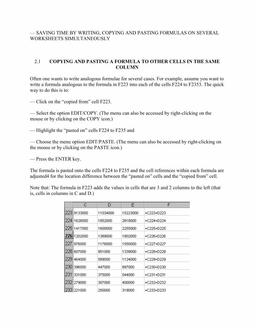
— SAVING TIME BY WRITING, COPYING AND PASTING FORMULAS ON SEVERAL WORKSHEETS SIMULTANEOUSLY
2.1 COPYING AND PASTING A FORMULA TO OTHER CELLS IN THE SAME COLUMN
Often one wants to write analogous formulae for several cases. For example, assume you want to write a formula analogous to the formula in F223 into each of the cells F224 to F2353. The quick way to do this is to: — Click on the “copied from” cell F223. — Select the option EDIT/COPY. (The menu can also be accessed by right-clicking on the mouse or by clicking on the COPY icon.) — Highlight the “pasted on” cells F224 to F235 and — Choose the menu option EDIT/PASTE. (The menu can also be accessed by right-clicking on the mouse or by clicking on the PASTE icon.) — Press the ENTER key. The formula is pasted onto the cells F224 to F235 and the cell references within each formula are adjusted4 for the location difference between the “pasted on” cells and the “copied from” cell. Note that: The formula in F223 adds the values in cells that are 3 and 2 columns to the left (that is, cells in columns in C and D.)
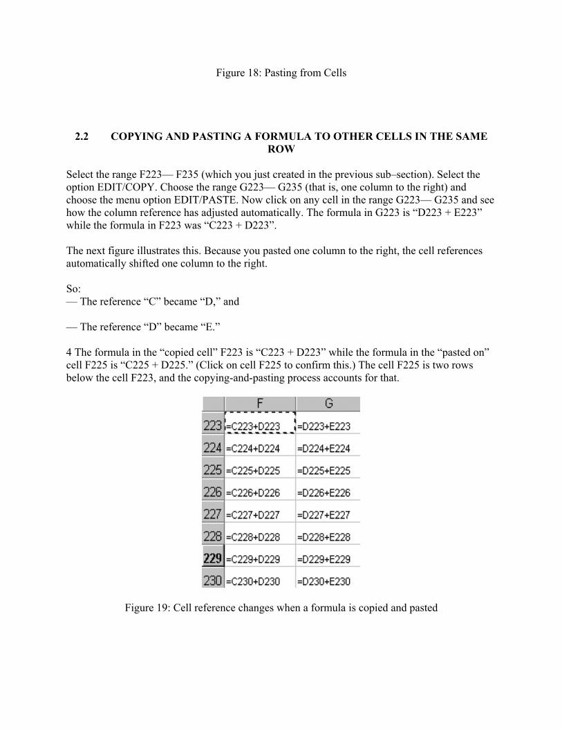
Figure 18: Pasting from Cells
2.2 COPYING AND PASTING A FORMULA TO OTHER CELLS IN THE SAME ROW
Select the range F223— F235 (which you just created in the previous sub–section). Select the option EDIT/COPY. Choose the range G223— G235 (that is, one column to the right) and choose the menu option EDIT/PASTE. Now click on any cell in the range G223— G235 and see how the column reference has adjusted automatically. The formula in G223 is “D223 + E223” while the formula in F223 was “C223 + D223”. The next figure illustrates this. Because you pasted one column to the right, the cell references automatically shifted one column to the right. So: — The reference “C” became “D,” and — The reference “D” became “E.” 4 The formula in the “copied cell” F223 is “C223 + D223” while the formula in the “pasted on” cell F225 is “C225 + D225.” (Click on cell F225 to confirm this.) The cell F225 is two rows below the cell F223, and the copying-and-pasting process accounts for that.
Figure 19: Cell reference changes when a formula is copied and pasted
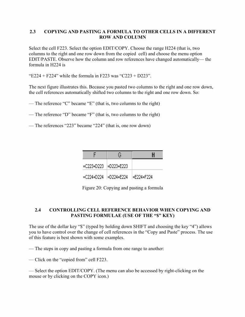
2.3 COPYING AND PASTING A FORMULA TO OTHER CELLS IN A DIFFERENT ROW AND COLUMN
Select the cell F223. Select the option EDIT/COPY. Choose the range H224 (that is, two columns to the right and one row down from the copied cell) and choose the menu option EDIT/PASTE. Observe how the column and row references have changed automatically— the formula in H224 is “E224 + F224” while the formula in F223 was “C223 + D223”. The next figure illustrates this. Because you pasted two columns to the right and one row down, the cell references automatically shifted two columns to the right and one row down. So: — The reference “C” became “E” (that is, two columns to the right) — The reference “D” became “F” (that is, two columns to the right) — The references “223” became “224” (that is, one row down)
Figure 20: Copying and pasting a formula
2.4 CONTROLLING CELL REFERENCE BEHAVIOR WHEN COPYING AND PASTING FORMULAE (USE OF THE “$” KEY)
The use of the dollar key “$” (typed by holding down SHIFT and choosing the key “4”) allows you to have control over the change of cell references in the “Copy and Paste” process. The use of this feature is best shown with some examples. — The steps in copy and pasting a formula from one range to another: — Click on the “copied from” cell F223. — Select the option EDIT/COPY. (The menu can also be accessed by right-clicking on the mouse or by clicking on the COPY icon.)
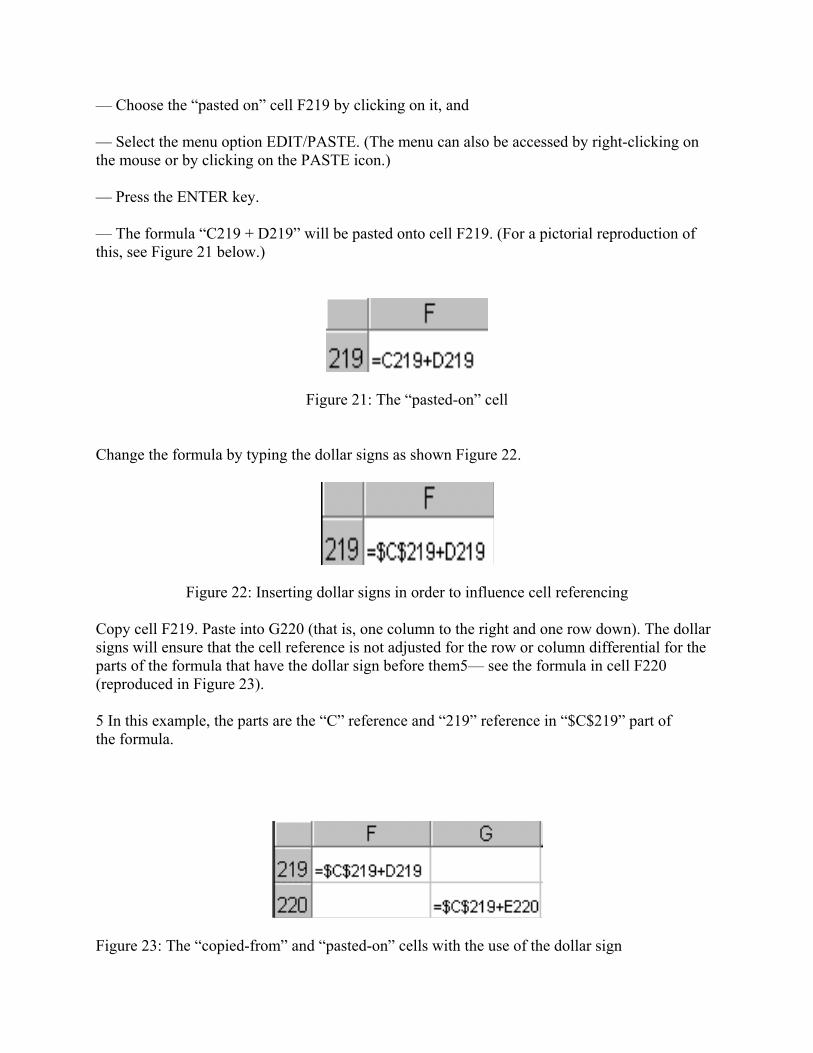
— Choose the “pasted on” cell F219 by clicking on it, and — Select the menu option EDIT/PASTE. (The menu can also be accessed by right-clicking on the mouse or by clicking on the PASTE icon.) — Press the ENTER key. — The formula “C219 + D219” will be pasted onto cell F219. (For a pictorial reproduction of this, see Figure 21 below.)
Figure 21: The “pasted-on” cell
Change the formula by typing the dollar signs as shown Figure 22.
Figure 22: Inserting dollar signs in order to influence cell referencing Copy cell F219. Paste into G220 (that is, one column to the right and one row down). The dollar signs will ensure that the cell reference is not adjusted for the row or column differential for the parts of the formula that have the dollar sign before them5— see the formula in cell F220 (reproduced in Figure 23). 5 In this example, the parts are the “C” reference and “219” reference in “$C$219” part of the formula.
Figure 23: The “copied-from” and “pasted-on” cells with the use of the dollar sign
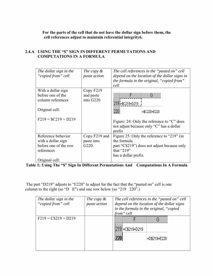
For the parts of the cell that do not have the dollar sign before them, the
cell references adjust to maintain referential integrity6.
2.4.A USING THE “$” SIGN IN DIFFERENT PERMUTATIONS AND
COMPUTATIONS IN A FORMULA
The dollar sign in the “copied from” cell
The copy & paste action
The cell references in the “pasted on” cell depend on the location of the dollar signs in the formula in the original, “copied from” cell
With a dollar sign before one of the column references Original cell: F219 = $C219 + D219
Copy F219 and paste into G220
Figure: 24: Only the reference to “C” does not adjust because only “C” has a dollar prefix
Reference behavior with a dollar sign before one of the row references Original cell:
Copy F219 and paste into G220.
Figure 25: Only the reference to “219” (in the formula part “C$219”) does not adjust because only that “219” has a dollar prefix
Table 1: Using The “$” Sign In Different Permutations And Computations In A Formula The part “D219” adjusts to “E220” to adjust for the fact that the “pasted on” cell is one column to the right (so “D�E") and one row below (so “219�220”.)
The dollar sign in the “copied from” cell
The copy & paste action
The cell references in the “pasted on” cell depend on the location of the dollar signs in the formula in the original, “copied from” cell
F219 = C$219 + D219
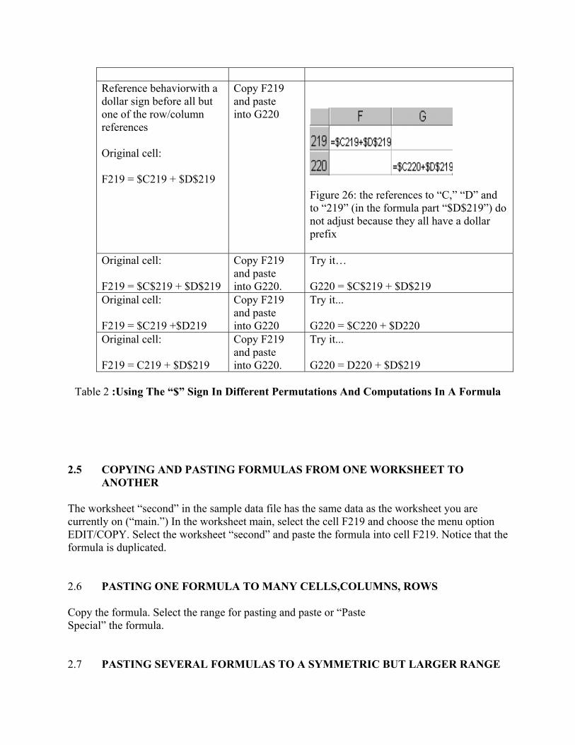
Reference behaviorwith a dollar sign before all but one of the row/column references Original cell: F219 = $C219 + $D$219
Copy F219 and paste into G220
Figure 26: the references to “C,” “D” and to “219” (in the formula part “$D$219”) do not adjust because they all have a dollar prefix
Original cell: F219 = $C$219 + $D$219
Copy F219 and paste into G220.
Try it… G220 = $C$219 + $D$219
Original cell: F219 = $C219 +$D219
Copy F219 and paste into G220
Try it... G220 = $C220 + $D220
Original cell: F219 = C219 + $D$219
Copy F219 and paste into G220.
Try it... G220 = D220 + $D$219
Table 2 :Using The “$” Sign In Different Permutations And Computations In A Formula
2.5 COPYING AND PASTING FORMULAS FROM ONE WORKSHEET TO
ANOTHER
The worksheet “second” in the sample data file has the same data as the worksheet you are currently on (“main.”) In the worksheet main, select the cell F219 and choose the menu option EDIT/COPY. Select the worksheet “second” and paste the formula into cell F219. Notice that the formula is duplicated. 2.6 PASTING ONE FORMULA TO MANY CELLS,COLUMNS, ROWS
Copy the formula. Select the range for pasting and paste or “Paste Special” the formula. 2.7 PASTING SEVERAL FORMULAS TO A SYMMETRIC BUT LARGER RANGE
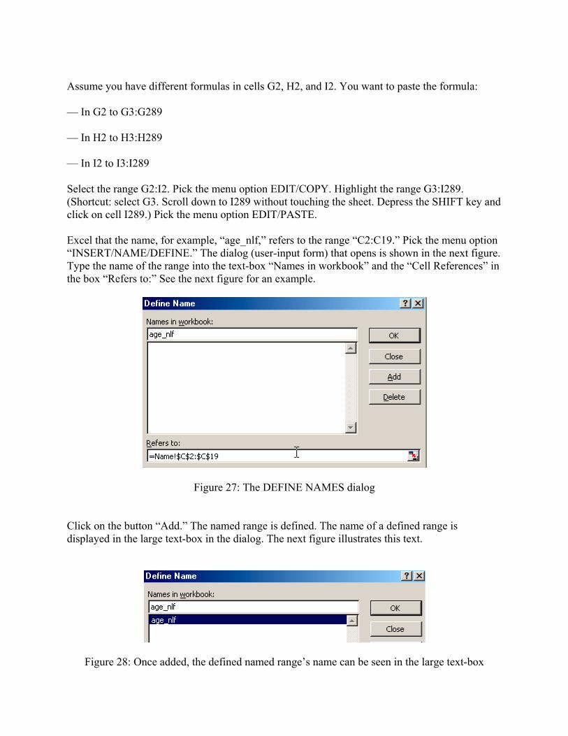
Assume you have different formulas in cells G2, H2, and I2. You want to paste the formula: — In G2 to G3:G289 — In H2 to H3:H289 — In I2 to I3:I289 Select the range G2:I2. Pick the menu option EDIT/COPY. Highlight the range G3:I289. (Shortcut: select G3. Scroll down to I289 without touching the sheet. Depress the SHIFT key and click on cell I289.) Pick the menu option EDIT/PASTE. Excel that the name, for example, “age_nlf,” refers to the range “C2:C19.” Pick the menu option “INSERT/NAME/DEFINE.” The dialog (user-input form) that opens is shown in the next figure. Type the name of the range into the text-box “Names in workbook” and the “Cell References” in the box “Refers to:” See the next figure for an example.
Figure 27: The DEFINE NAMES dialog
Click on the button “Add.” The named range is defined. The name of a defined range is displayed in the large text-box in the dialog. The next figure illustrates this text.
Figure 28: Once added, the defined named range’s name can be seen in the large text-box
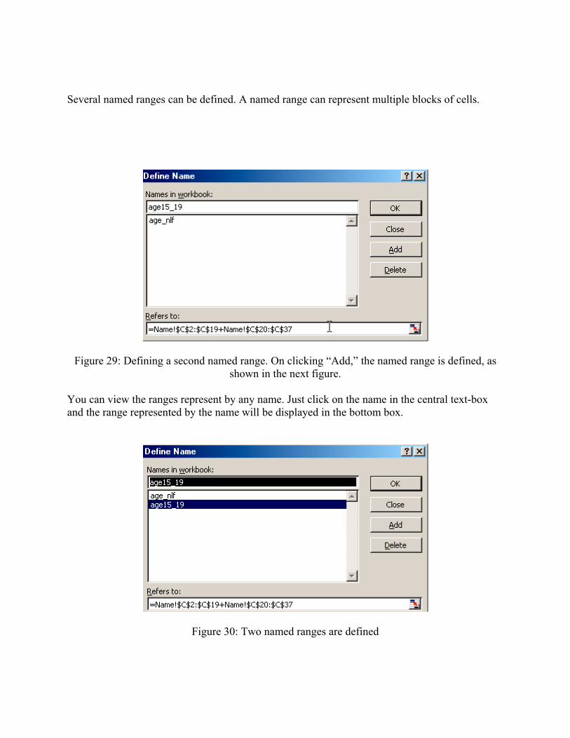
Several named ranges can be defined. A named range can represent multiple blocks of cells.
Figure 29: Defining a second named range. On clicking “Add,” the named range is defined, as shown in the next figure.
You can view the ranges represent by any name. Just click on the name in the central text-box and the range represented by the name will be displayed in the bottom box.
Figure 30: Two named ranges are defined
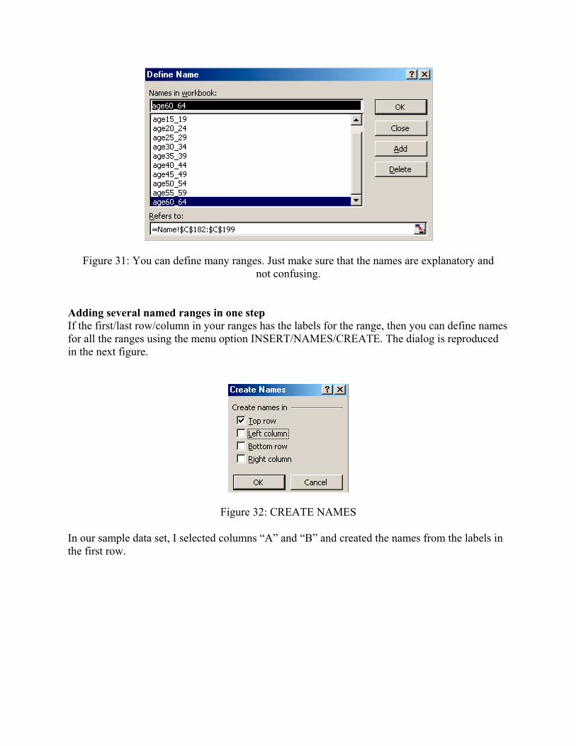
Figure 31: You can define many ranges. Just make sure that the names are explanatory and not confusing.
Adding several named ranges in one step If the first/last row/column in your ranges has the labels for the range, then you can define names for all the ranges using the menu option INSERT/NAMES/CREATE. The dialog is reproduced in the next figure.
Figure 32: CREATE NAMES
In our sample data set, I selected columns “A” and “B” and created the names from the labels in the first row.
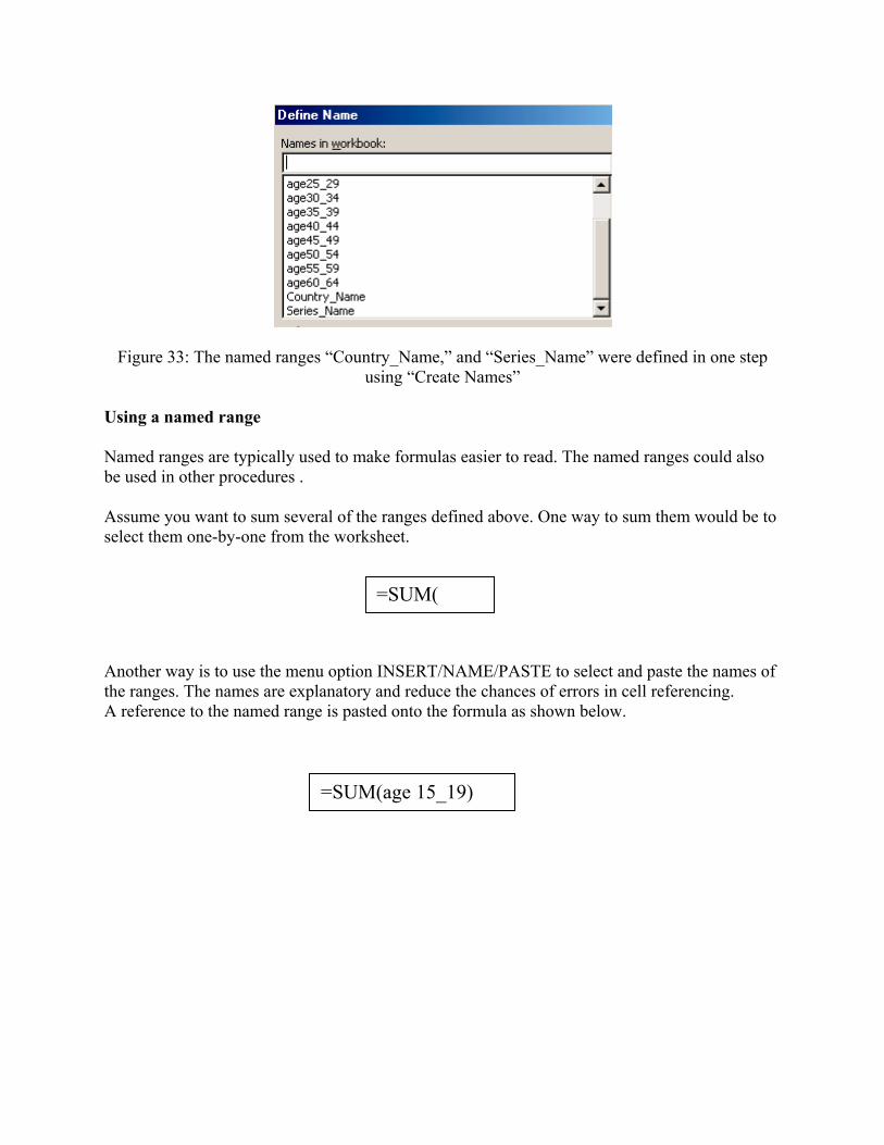
Figure 33: The named ranges “Country_Name,” and “Series_Name” were defined in one step using “Create Names”
Using a named range Named ranges are typically used to make formulas easier to read. The named ranges could also be used in other procedures . Assume you want to sum several of the ranges defined above. One way to sum them would be to select them one-by-one from the worksheet.
Another way is to use the menu option INSERT/NAME/PASTE to select and paste the names of the ranges. The names are explanatory and reduce the chances of errors in cell referencing. A reference to the named range is pasted onto the formula as shown below.
=SUM(
=SUM(age 15_19)
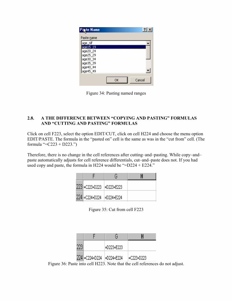
Figure 34: Pasting named ranges
2.8. A THE DIFFERENCE BETWEEN “COPYING AND PASTING” FORMULAS
AND “CUTTING AND PASTING” FORMULAS Click on cell F223, select the option EDIT/CUT, click on cell H224 and choose the menu option EDIT/PASTE. The formula in the “pasted on” cell is the same as was in the “cut from” cell. (The formula “=C223 + D223.”) Therefore, there is no change in the cell references after cutting–and–pasting. While copy–and–paste automatically adjusts for cell reference differentials, cut–and–paste does not. If you had used copy and paste, the formula in H224 would be “=D224 + E224.”
Figure 35: Cut from cell F223
Figure 36: Paste into cell H223. Note that the cell references do not adjust.
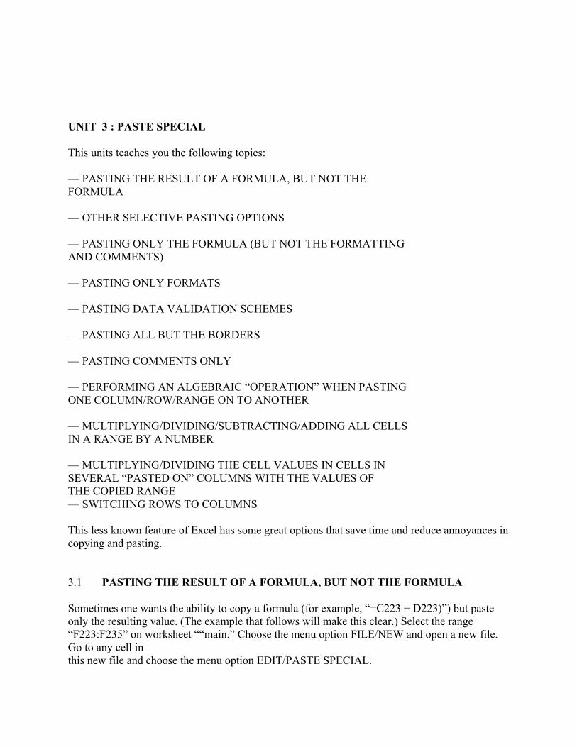
UNIT 3 : PASTE SPECIAL This units teaches you the following topics: — PASTING THE RESULT OF A FORMULA, BUT NOT THE FORMULA — OTHER SELECTIVE PASTING OPTIONS — PASTING ONLY THE FORMULA (BUT NOT THE FORMATTING AND COMMENTS) — PASTING ONLY FORMATS — PASTING DATA VALIDATION SCHEMES — PASTING ALL BUT THE BORDERS — PASTING COMMENTS ONLY — PERFORMING AN ALGEBRAIC “OPERATION” WHEN PASTING ONE COLUMN/ROW/RANGE ON TO ANOTHER — MULTIPLYING/DIVIDING/SUBTRACTING/ADDING ALL CELLS IN A RANGE BY A NUMBER — MULTIPLYING/DIVIDING THE CELL VALUES IN CELLS IN SEVERAL “PASTED ON” COLUMNS WITH THE VALUES OF THE COPIED RANGE — SWITCHING ROWS TO COLUMNS This less known feature of Excel has some great options that save time and reduce annoyances in copying and pasting. 3.1 PASTING THE RESULT OF A FORMULA, BUT NOT THE FORMULA
Sometimes one wants the ability to copy a formula (for example, “=C223 + D223)”) but paste only the resulting value. (The example that follows will make this clear.) Select the range “F223:F235” on worksheet ““main.” Choose the menu option FILE/NEW and open a new file. Go to any cell in this new file and choose the menu option EDIT/PASTE SPECIAL.
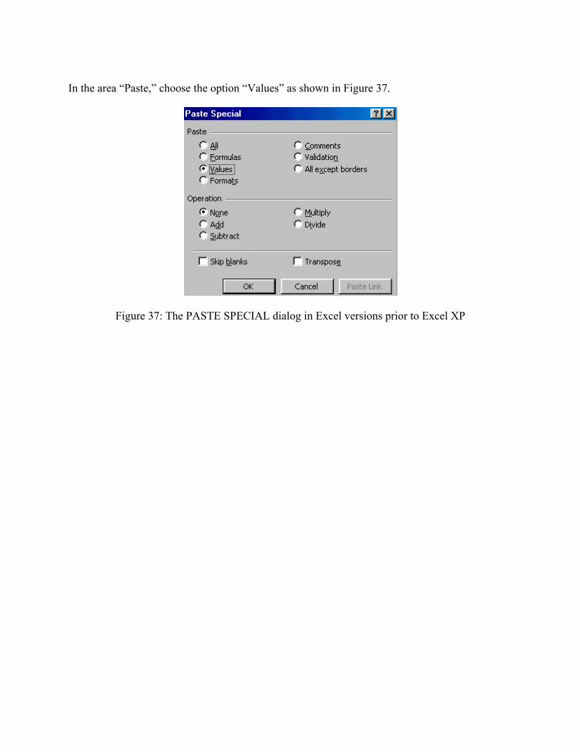
In the area “Paste,” choose the option “Values” as shown in Figure 37.
Figure 37: The PASTE SPECIAL dialog in Excel versions prior to Excel XP
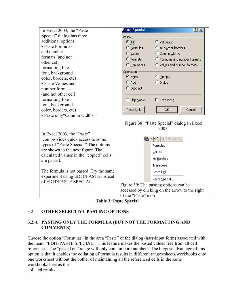
In Excel 2003, the “Paste Special” dialog has three additional options: • Paste Formulas and number formats (and not other cell formatting like font, background color, borders, etc) • Paste Values and number formats (and not other cell formatting like font, background color, borders, etc) • Paste only“Column widths.”
Figure 38: “Paste Special” dialog In Excel
2003, In Excel 2003, the “Paste” icon provides quick access to some types of “Paste Special.” The options are shown in the next figure. The calculated values in the “copied” cells are pasted. The formula is not pasted. Try the same experiment using EDIT/PASTE instead of EDIT/PASTE SPECIAL.
Figure 39: The pasting options can be accessed by clicking on the arrow to the right of the “Paste” icon
Table 3: Paste Special
3.2 OTHER SELECTIVE PASTING OPTIONS 3.2.A PASTING ONLY THE FORMULA (BUT NOT THE FORMATTING AND
COMMENTS) Choose the option “Formulas” in the area “Paste” of the dialog (user-input form) associated with the menu “EDIT/PASTE SPECIAL.” This feature makes the pasted values free from all cell references. The “pasted on” range will only contain pure numbers. The biggest advantage of this option is that it enables the collating of formula results in different ranges/sheets/workbooks onto one worksheet without the bother of maintaining all the referenced cells in the same workbook/sheet as the collated results.
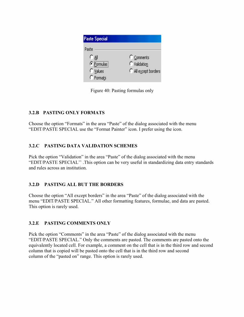
Figure 40: Pasting formulas only
3.2.B PASTING ONLY FORMATS Choose the option “Formats” in the area “Paste” of the dialog associated with the menu “EDIT/PASTE SPECIAL use the “Format Painter” icon. I prefer using the icon. 3.2.C PASTING DATA VALIDATION SCHEMES Pick the option “Validation” in the area “Paste” of the dialog associated with the menu “EDIT/PASTE SPECIAL’’ .This option can be very useful in standardizing data entry standards and rules across an institution. 3.2.D PASTING ALL BUT THE BORDERS Choose the option “All except borders” in the area “Paste” of the dialog associated with the menu “EDIT/PASTE SPECIAL.” All other formatting features, formulae, and data are pasted. This option is rarely used. 3.2.E PASTING COMMENTS ONLY Pick the option “Comments” in the area “Paste” of the dialog associated with the menu “EDIT/PASTE SPECIAL.” Only the comments are pasted. The comments are pasted onto the equivalently located cell. For example, a comment on the cell that is in the third row and second column that is copied will be pasted onto the cell that is in the third row and second column of the “pasted on” range. This option is rarely used.
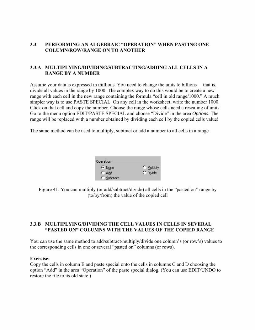
3.3 PERFORMING AN ALGEBRAIC “OPERATION” WHEN PASTING ONE
COLUMN/ROW/RANGE ON TO ANOTHER 3.3.A MULTIPLYING/DIVIDING/SUBTRACTING/ADDING ALL CELLS IN A
RANGE BY A NUMBER Assume your data is expressed in millions. You need to change the units to billions— that is, divide all values in the range by 1000. The complex way to do this would be to create a new range with each cell in the new range containing the formula “cell in old range/1000.” A much simpler way is to use PASTE SPECIAL. On any cell in the worksheet, write the number 1000. Click on that cell and copy the number. Choose the range whose cells need a rescaling of units. Go to the menu option EDIT/PASTE SPECIAL and choose “Divide” in the area Options. The range will be replaced with a number obtained by dividing each cell by the copied cells value! The same method can be used to multiply, subtract or add a number to all cells in a range
Figure 41: You can multiply (or add/subtract/divide) all cells in the “pasted on” range by (to/by/from) the value of the copied cell
3.3.B MULTIPLYING/DIVIDING THE CELL VALUES IN CELLS IN SEVERAL
“PASTED ON” COLUMNS WITH THE VALUES OF THE COPIED RANGE You can use the same method to add/subtract/multiply/divide one column’s (or row’s) values to the corresponding cells in one or several “pasted on” columns (or rows). Exercise: Copy the cells in column E and paste special onto the cells in columns C and D choosing the option “Add” in the area “Operation” of the paste special dialog. (You can use EDIT/UNDO to restore the file to its old state.)
3.4 SWITCHING ROWS TO COLUMNS Choose any option in the “Paste” and “Operations” areas and choose the option “Transpose.” If pasting a range with many columns and rows you may prefer to paste onto one cell to avoid getting the error “Copy and Paste areas are in different shapes.” UNIT 4 INSERTING FUNCTIONS This unit teaches you the following topics: — A SIMPLE FUNCTION — FUNCTIONS THAT NEED MULTIPLE RANGE REFERENCES — WRITING A “FUNCTION WITHIN A FUNCTION“ — NEW IN EXCEL 2003 — RECOMMENDED FUNCTIONS IN THE FUNCTION WIZARD — EXPANDED AUTOSUM FUNCTIONALITY — FORMULA EVALUATOR — FORMULA ERROR CHECKING 4.1 BASICS Excel has many in–built functions. The functions may be inserted into a formula. Accessing the functions dialog/wizard
(a) select the menu path INSERT/FUNCTION or
(b) click on the function icon (see Figure 42)
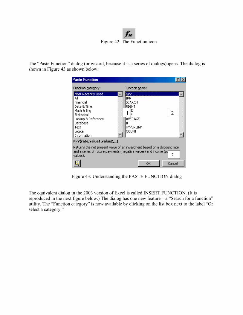
Figure 42: The Function icon
The “Paste Function” dialog (or wizard, because it is a series of dialogs)opens. The dialog is shown in Figure 43 as shown below:
Figure 43: Understanding the PASTE FUNCTION dialog
The equivalent dialog in the 2003 version of Excel is called INSERT FUNCTION. (It is reproduced in the next figure below.) The dialog has one new feature—a “Search for a function” utility. The “Function category” is now available by clicking on the list box next to the label “Or select a category.”
2 1
3
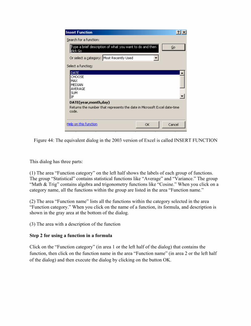
Figure 44: The equivalent dialog in the 2003 version of Excel is called INSERT FUNCTION
This dialog has three parts: (1) The area “Function category” on the left half shows the labels of each group of functions. The group “Statistical” contains statistical functions like “Average” and “Variance.” The group “Math & Trig” contains algebra and trigonometry functions like “Cosine.” When you click on a category name, all the functions within the group are listed in the area “Function name.” (2) The area “Function name” lists all the functions within the category selected in the area “Function category.” When you click on the name of a function, its formula, and description is shown in the gray area at the bottom of the dialog. (3) The area with a description of the function Step 2 for using a function in a formula Click on the “Function category” (in area 1 or the left half of the dialog) that contains the function, then click on the function name in the area “Function name” (in area 2 or the left half of the dialog) and then execute the dialog by clicking on the button OK.
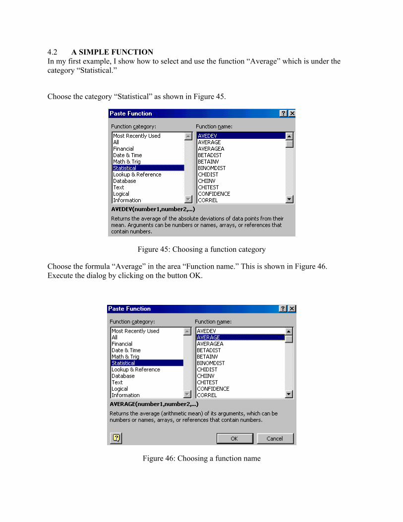
4.2 A SIMPLE FUNCTION In my first example, I show how to select and use the function “Average” which is under the category “Statistical.”
Choose the category “Statistical” as shown in Figure 45.
Figure 45: Choosing a function category
Choose the formula “Average” in the area “Function name.” This is shown in Figure 46. Execute the dialog by clicking on the button OK.
Figure 46: Choosing a function name
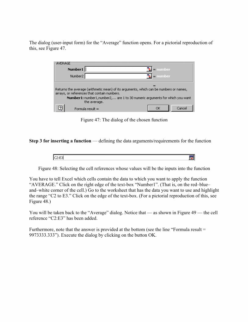
The dialog (user-input form) for the “Average” function opens. For a pictorial reproduction of this, see Figure 47.
Figure 47: The dialog of the chosen function
Step 3 for inserting a function — defining the data arguments/requirements for the function
Figure 48: Selecting the cell references whose values will be the inputs into the function
You have to tell Excel which cells contain the data to which you want to apply the function “AVERAGE.” Click on the right edge of the text-box “Number1”. (That is, on the red–blue–and–white corner of the cell.) Go to the worksheet that has the data you want to use and highlight the range “C2 to E3.” Click on the edge of the text-box. (For a pictorial reproduction of this, see Figure 48.) You will be taken back to the “Average” dialog. Notice that — as shown in Figure 49 — the cell reference “C2:E3” has been added. Furthermore, note that the answer is provided at the bottom (see the line “Formula result = 9973333.333”). Execute the dialog by clicking on the button OK.
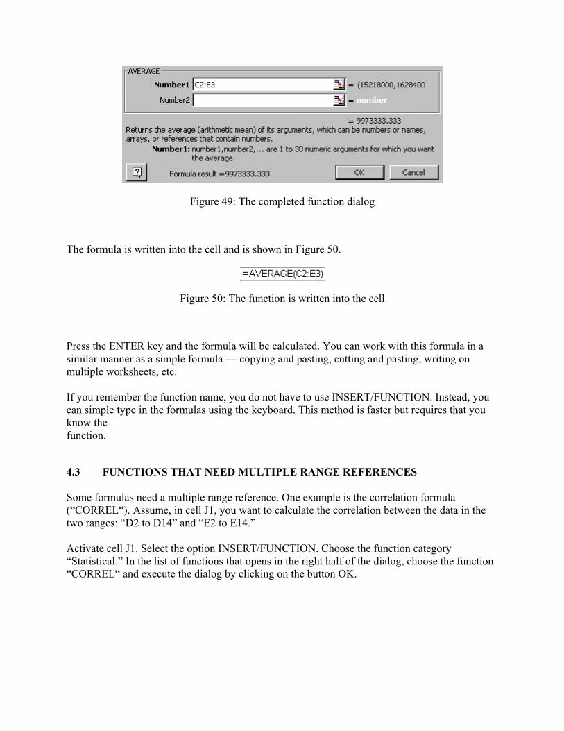
Figure 49: The completed function dialog
The formula is written into the cell and is shown in Figure 50.
Figure 50: The function is written into the cell
Press the ENTER key and the formula will be calculated. You can work with this formula in a similar manner as a simple formula — copying and pasting, cutting and pasting, writing on multiple worksheets, etc. If you remember the function name, you do not have to use INSERT/FUNCTION. Instead, you can simple type in the formulas using the keyboard. This method is faster but requires that you know the function.
4.3 FUNCTIONS THAT NEED MULTIPLE RANGE REFERENCES Some formulas need a multiple range reference. One example is the correlation formula (“CORREL“). Assume, in cell J1, you want to calculate the correlation between the data in the two ranges: “D2 to D14” and “E2 to E14.” Activate cell J1. Select the option INSERT/FUNCTION. Choose the function category “Statistical.” In the list of functions that opens in the right half of the dialog, choose the function “CORREL“ and execute the dialog by clicking on the button OK.
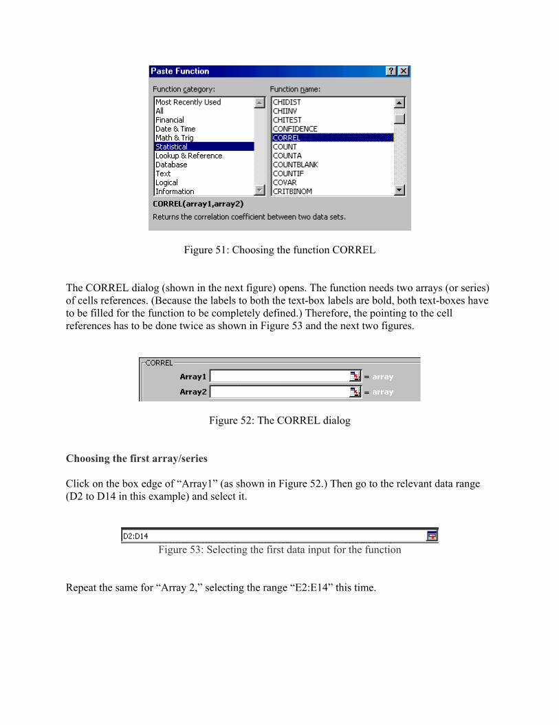
Figure 51: Choosing the function CORREL
The CORREL dialog (shown in the next figure) opens. The function needs two arrays (or series) of cells references. (Because the labels to both the text-box labels are bold, both text-boxes have to be filled for the function to be completely defined.) Therefore, the pointing to the cell references has to be done twice as shown in Figure 53 and the next two figures.
Figure 52: The CORREL dialog
Choosing the first array/series Click on the box edge of “Array1” (as shown in Figure 52.) Then go to the relevant data range (D2 to D14 in this example) and select it.
Figure 53: Selecting the first data input for the function
Repeat the same for “Array 2,” selecting the range “E2:E14” this time.
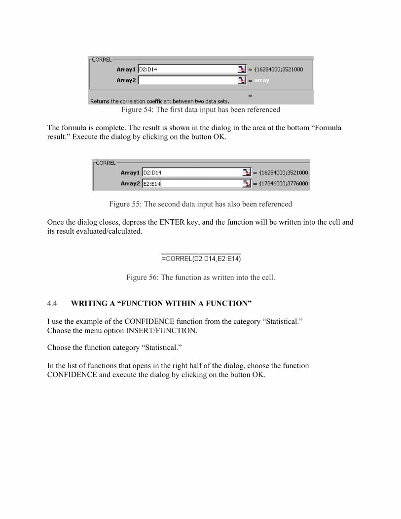
Figure 54: The first data input has been referenced
The formula is complete. The result is shown in the dialog in the area at the bottom “Formula result.” Execute the dialog by clicking on the button OK.
Figure 55: The second data input has also been referenced
Once the dialog closes, depress the ENTER key, and the function will be written into the cell and its result evaluated/calculated.
Figure 56: The function as written into the cell.
4.4 WRITING A “FUNCTION WITHIN A FUNCTION” I use the example of the CONFIDENCE function from the category “Statistical.” Choose the menu option INSERT/FUNCTION.
Choose the function category “Statistical.” In the list of functions that opens in the right half of the dialog, choose the function CONFIDENCE and execute the dialog by clicking on the button OK.
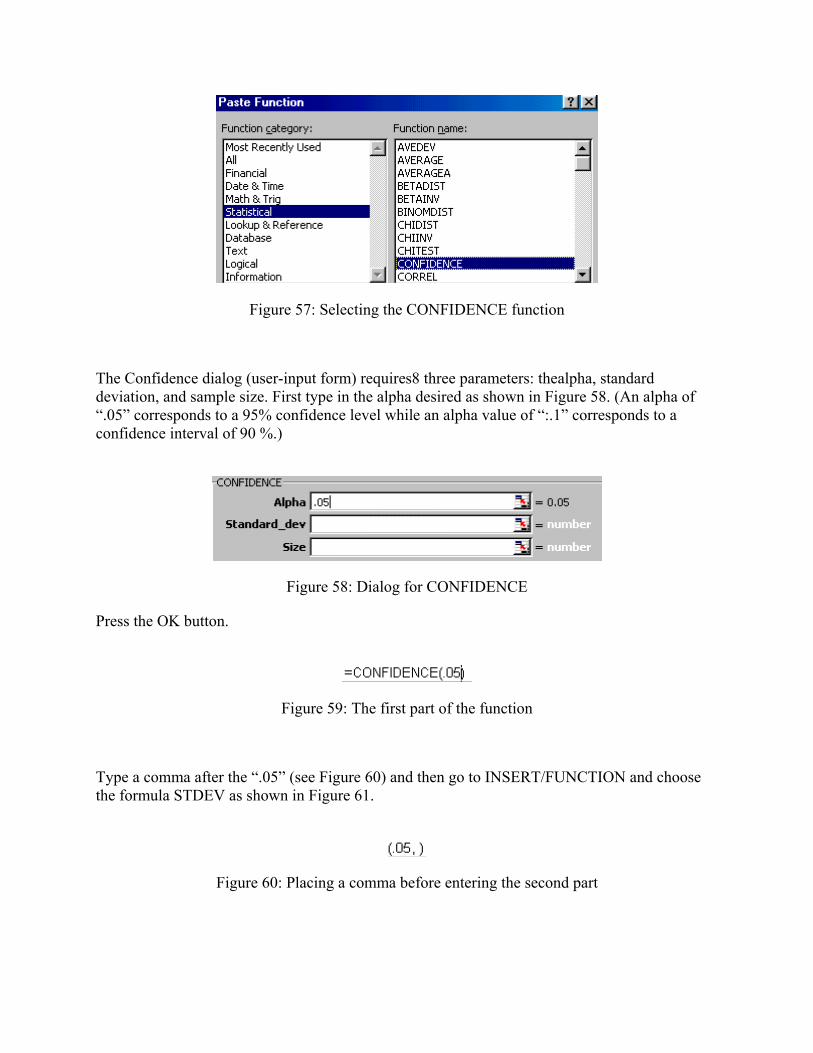
Figure 57: Selecting the CONFIDENCE function
The Confidence dialog (user-input form) requires8 three parameters: thealpha, standard deviation, and sample size. First type in the alpha desired as shown in Figure 58. (An alpha of “.05” corresponds to a 95% confidence level while an alpha value of “:.1” corresponds to a confidence interval of 90 %.)
Figure 58: Dialog for CONFIDENCE
Press the OK button.
Figure 59: The first part of the function
Type a comma after the “.05” (see Figure 60) and then go to INSERT/FUNCTION and choose the formula STDEV as shown in Figure 61.
Figure 60: Placing a comma before entering the second part
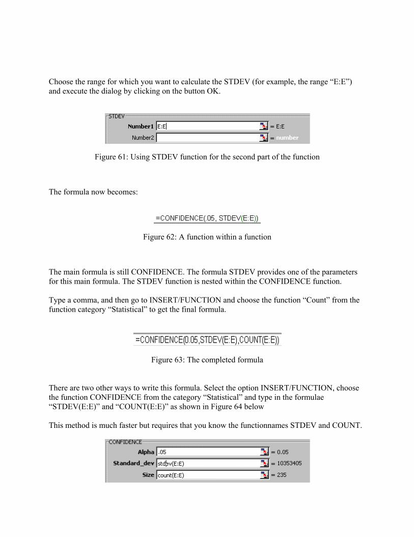
Choose the range for which you want to calculate the STDEV (for example, the range “E:E”) and execute the dialog by clicking on the button OK.
Figure 61: Using STDEV function for the second part of the function
The formula now becomes:
Figure 62: A function within a function
The main formula is still CONFIDENCE. The formula STDEV provides one of the parameters for this main formula. The STDEV function is nested within the CONFIDENCE function. Type a comma, and then go to INSERT/FUNCTION and choose the function “Count” from the function category “Statistical” to get the final formula.
Figure 63: The completed formula
There are two other ways to write this formula. Select the option INSERT/FUNCTION, choose the function CONFIDENCE from the category “Statistical” and type in the formulae “STDEV(E:E)” and “COUNT(E:E)” as shown in Figure 64 below This method is much faster but requires that you know the functionnames STDEV and COUNT.
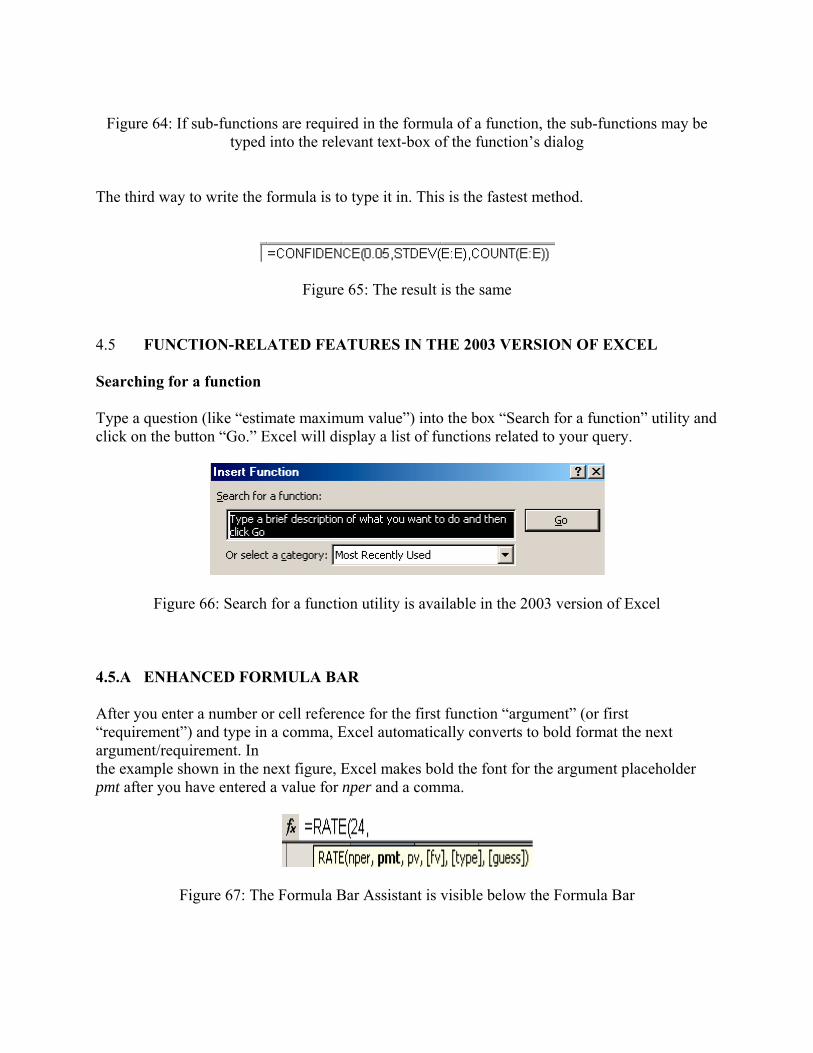
Figure 64: If sub-functions are required in the formula of a function, the sub-functions may be
typed into the relevant text-box of the function’s dialog
The third way to write the formula is to type it in. This is the fastest method.
Figure 65: The result is the same
4.5 FUNCTION-RELATED FEATURES IN THE 2003 VERSION OF EXCEL Searching for a function Type a question (like “estimate maximum value”) into the box “Search for a function” utility and click on the button “Go.” Excel will display a list of functions related to your query.
Figure 66: Search for a function utility is available in the 2003 version of Excel
4.5.A ENHANCED FORMULA BAR After you enter a number or cell reference for the first function “argument” (or first “requirement”) and type in a comma, Excel automatically converts to bold format the next argument/requirement. In the example shown in the next figure, Excel makes bold the font for the argument placeholder pmt after you have entered a value for nper and a comma.
Figure 67: The Formula Bar Assistant is visible below the Formula Bar
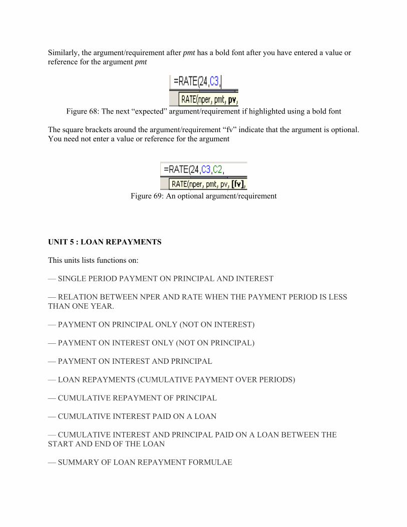
Similarly, the argument/requirement after pmt has a bold font after you have entered a value or reference for the argument pmt
Figure 68: The next “expected” argument/requirement if highlighted using a bold font
The square brackets around the argument/requirement “fv” indicate that the argument is optional. You need not enter a value or reference for the argument
Figure 69: An optional argument/requirement
UNIT 5 : LOAN REPAYMENTS This units lists functions on: — SINGLE PERIOD PAYMENT ON PRINCIPAL AND INTEREST — RELATION BETWEEN NPER AND RATE WHEN THE PAYMENT PERIOD IS LESS THAN ONE YEAR. — PAYMENT ON PRINCIPAL ONLY (NOT ON INTEREST) — PAYMENT ON INTEREST ONLY (NOT ON PRINCIPAL) — PAYMENT ON INTEREST AND PRINCIPAL — LOAN REPAYMENTS (CUMULATIVE PAYMENT OVER PERIODS) — CUMULATIVE REPAYMENT OF PRINCIPAL — CUMULATIVE INTEREST PAID ON A LOAN — CUMULATIVE INTEREST AND PRINCIPAL PAID ON A LOAN BETWEEN THE START AND END OF THE LOAN — SUMMARY OF LOAN REPAYMENT FORMULAE
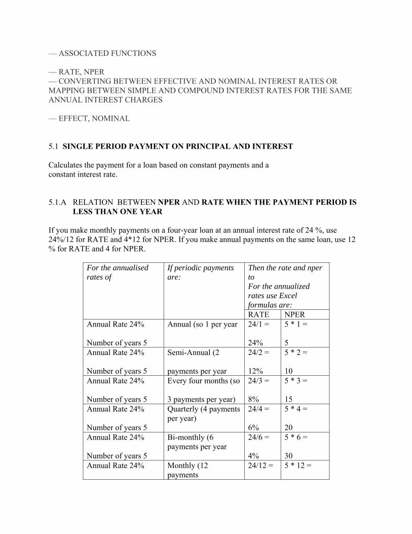
— ASSOCIATED FUNCTIONS — RATE, NPER — CONVERTING BETWEEN EFFECTIVE AND NOMINAL INTEREST RATES OR MAPPING BETWEEN SIMPLE AND COMPOUND INTEREST RATES FOR THE SAME ANNUAL INTEREST CHARGES — EFFECT, NOMINAL 5.1 SINGLE PERIOD PAYMENT ON PRINCIPAL AND INTEREST Calculates the payment for a loan based on constant payments and a constant interest rate. 5.1.A RELATION BETWEEN NPER AND RATE WHEN THE PAYMENT PERIOD IS
LESS THAN ONE YEAR If you make monthly payments on a four-year loan at an annual interest rate of 24 %, use 24%/12 for RATE and 4*12 for NPER. If you make annual payments on the same loan, use 12 % for RATE and 4 for NPER.
For the annualised rates of
If periodic payments are:
Then the rate and nper to For the annualized rates use Excel formulas are: RATE NPER
Annual Rate 24% Number of years 5
Annual (so 1 per year 24/1 = 24%
5 * 1 = 5
Annual Rate 24% Number of years 5
Semi-Annual (2 payments per year
24/2 = 12%
5 * 2 = 10
Annual Rate 24% Number of years 5
Every four months (so 3 payments per year)
24/3 = 8%
5 * 3 = 15
Annual Rate 24% Number of years 5
Quarterly (4 payments per year)
24/4 = 6%
5 * 4 = 20
Annual Rate 24% Number of years 5
Bi-monthly (6 payments per year
24/6 = 4%
5 * 6 = 30
Annual Rate 24%
Monthly (12 payments
24/12 =
5 * 12 =
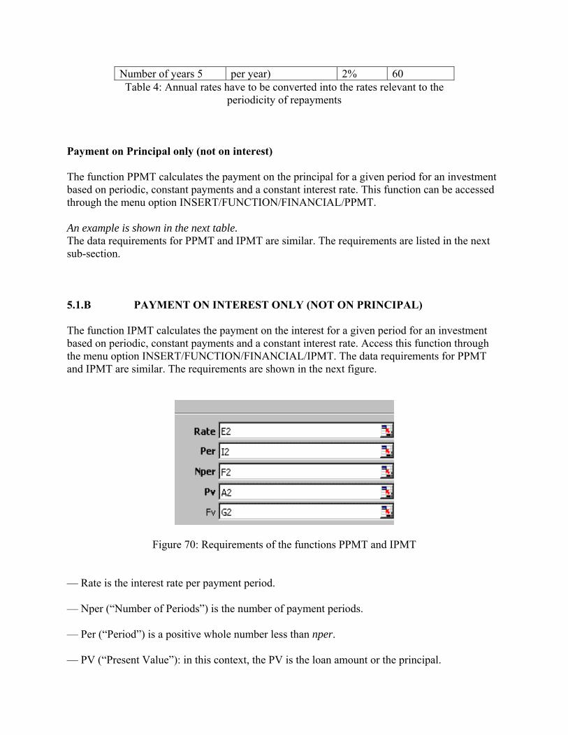
Number of years 5 per year) 2% 60 Table 4: Annual rates have to be converted into the rates relevant to the
periodicity of repayments
Payment on Principal only (not on interest) The function PPMT calculates the payment on the principal for a given period for an investment based on periodic, constant payments and a constant interest rate. This function can be accessed through the menu option INSERT/FUNCTION/FINANCIAL/PPMT. An example is shown in the next table. The data requirements for PPMT and IPMT are similar. The requirements are listed in the next sub-section.
5.1.B PAYMENT ON INTEREST ONLY (NOT ON PRINCIPAL) The function IPMT calculates the payment on the interest for a given period for an investment based on periodic, constant payments and a constant interest rate. Access this function through the menu option INSERT/FUNCTION/FINANCIAL/IPMT. The data requirements for PPMT and IPMT are similar. The requirements are shown in the next figure.
Figure 70: Requirements of the functions PPMT and IPMT — Rate is the interest rate per payment period. — Nper (“Number of Periods”) is the number of payment periods. — Per (“Period”) is a positive whole number less than nper. — PV (“Present Value”): in this context, the PV is the loan amount or the principal.
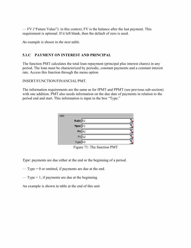
— FV (“Future Value”): in this context, FV is the balance after the last payment. This requirement is optional. If it left blank, then the default of zero is used. An example is shown in the next table. 5.1.C PAYMENT ON INTEREST AND PRINCIPAL The function PMT calculates the total loan repayment (principal plus interest chares) in any period. The loan must be characterized by periodic, constant payments and a constant interest rate. Access this function through the menu option INSERT/FUNCTION/FINANCIAL/PMT. The information requirements are the same as for IPMT and PPMT (see previous sub-section) with one addition. PMT also needs information on the due date of payments in relation to the period end and start. This information is input in the box “Type.”
Figure 71: The function PMT
Type: payments are due either at the end or the beginning of a period. — Type = 0 or omitted, if payments are due at the end. — Type = 1, if payments are due at the beginning An example is shown in table at the end of this unit
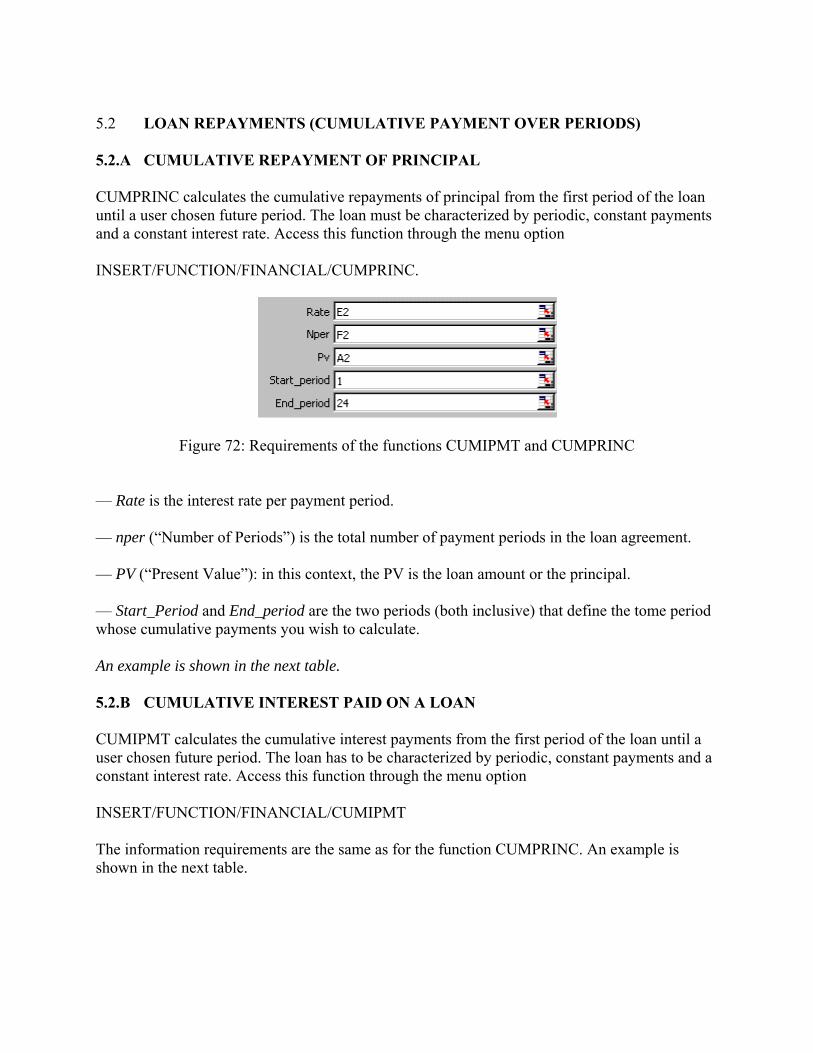
5.2 LOAN REPAYMENTS (CUMULATIVE PAYMENT OVER PERIODS) 5.2.A CUMULATIVE REPAYMENT OF PRINCIPAL CUMPRINC calculates the cumulative repayments of principal from the first period of the loan until a user chosen future period. The loan must be characterized by periodic, constant payments and a constant interest rate. Access this function through the menu option INSERT/FUNCTION/FINANCIAL/CUMPRINC.
Figure 72: Requirements of the functions CUMIPMT and CUMPRINC
— Rate is the interest rate per payment period. — nper (“Number of Periods”) is the total number of payment periods in the loan agreement. — PV (“Present Value”): in this context, the PV is the loan amount or the principal. — Start_Period and End_period are the two periods (both inclusive) that define the tome period whose cumulative payments you wish to calculate. An example is shown in the next table. 5.2.B CUMULATIVE INTEREST PAID ON A LOAN CUMIPMT calculates the cumulative interest payments from the first period of the loan until a user chosen future period. The loan has to be characterized by periodic, constant payments and a constant interest rate. Access this function through the menu option INSERT/FUNCTION/FINANCIAL/CUMIPMT The information requirements are the same as for the function CUMPRINC. An example is shown in the next table.
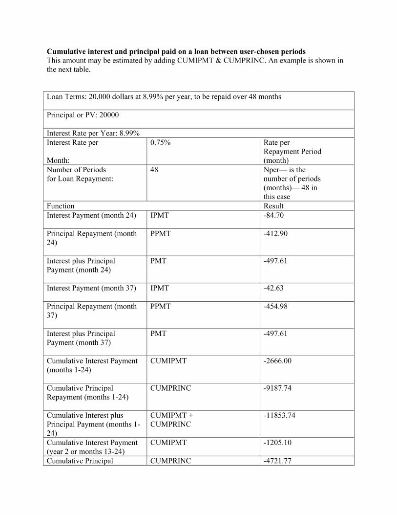
Cumulative interest and principal paid on a loan between user-chosen periods This amount may be estimated by adding CUMIPMT & CUMPRINC. An example is shown in the next table. Loan Terms: 20,000 dollars at 8.99% per year, to be repaid over 48 months Principal or PV: 20000 Interest Rate per Year: 8.99% Interest Rate per Month:
0.75% Rate per Repayment Period (month)
Number of Periods for Loan Repayment:
48 Nper— is the number of periods (months)— 48 in this case
Function Result Interest Payment (month 24)
IPMT -84.70
Principal Repayment (month 24)
PPMT -412.90
Interest plus Principal Payment (month 24)
PMT -497.61
Interest Payment (month 37)
IPMT -42.63
Principal Repayment (month 37)
PPMT -454.98
Interest plus Principal Payment (month 37)
PMT -497.61
Cumulative Interest Payment (months 1-24)
CUMIPMT -2666.00
Cumulative Principal Repayment (months 1-24)
CUMPRINC -9187.74
Cumulative Interest plus Principal Payment (months 1-24)
CUMIPMT + CUMPRINC
-11853.74
Cumulative Interest Payment (year 2 or months 13-24)
CUMIPMT -1205.10
Cumulative Principal CUMPRINC -4721.77
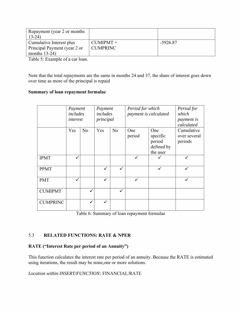
Repayment (year 2 or months 13-24) Cumulative Interest plus Principal Payment (year 2 or months 13-24)
CUMIPMT + CUMPRINC
-5926.87
Table 5: Example of a car loan. Note that the total repayments are the same in months 24 and 37, the share of interest goes down over time as more of the principal is repaid Summary of loan repayment formulae
Payment includes interest
Payment includes principal
Period for which payment is calculated
Period for which payment is calculated
Yes No Yes No One period
One specific period defined by the user
Cumulative over several periods
IPMT
PPMT
PMT
CUMIPMT
CUMPRINC
Table 6: Summary of loan repayment formulae
5.3 RELATED FUNCTIONS: RATE & NPER RATE (“Interest Rate per period of an Annuity”) This function calculates the interest rate per period of an annuity. Because the RATE is estimated using iterations, the result may be none,one or more solutions. Location within INSERT/FUNCTION: FINANCIAL/RATE
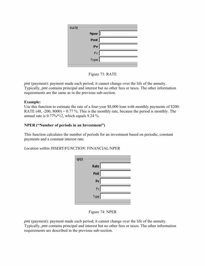
Figure 73: RATE pmt (payment): payment made each period; it cannot change over the life of the annuity. Typically, pmt contains principal and interest but no other fees or taxes. The other information requirements are the same as in the previous sub-section. Example: Use this function to estimate the rate of a four-year $8,000 loan with monthly payments of $200: RATE (48, -200, 8000) = 0.77 %. This is the monthly rate, because the period is monthly. The annual rate is 0.77%*12, which equals 9.24 %. NPER (“Number of periods in an Investment”) This function calculates the number of periods for an investment based on periodic, constant payments and a constant interest rate. Location within INSERT/FUNCTION: FINANCIAL/NPER
Figure 74: NPER
pmt (payment): payment made each period; it cannot change over the life of the annuity. Typically, pmt contains principal and interest but no other fees or taxes. The other information requirements are described in the previous sub-section.
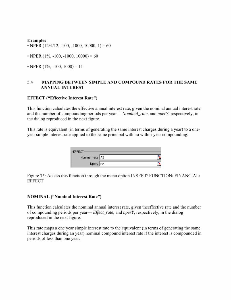
Examples • NPER (12%/12, -100, -1000, 10000, 1) = 60 • NPER (1%, -100, -1000, 10000) = 60 • NPER (1%, -100, 1000) = 11 5.4 MAPPING BETWEEN SIMPLE AND COMPOUND RATES FOR THE SAME
ANNUAL INTEREST EFFECT (“Effective Interest Rate”) This function calculates the effective annual interest rate, given the nominal annual interest rate and the number of compounding periods per year— Nominal_rate, and nperY, respectively, in the dialog reproduced in the next figure. This rate is equivalent (in terms of generating the same interest charges during a year) to a one-year simple interest rate applied to the same principal with no within-year compounding.
Figure 75: Access this function through the menu option INSERT/ FUNCTION/ FINANCIAL/ EFFECT NOMINAL (“Nominal Interest Rate”) This function calculates the nominal annual interest rate, given theeffective rate and the number of compounding periods per year— Effect_rate, and nperY, respectively, in the dialog reproduced in the next figure. This rate maps a one year simple interest rate to the equivalent (in terms of generating the same interest charges during an year) nominal compound interest rate if the interest is compounded in periods of less than one year.
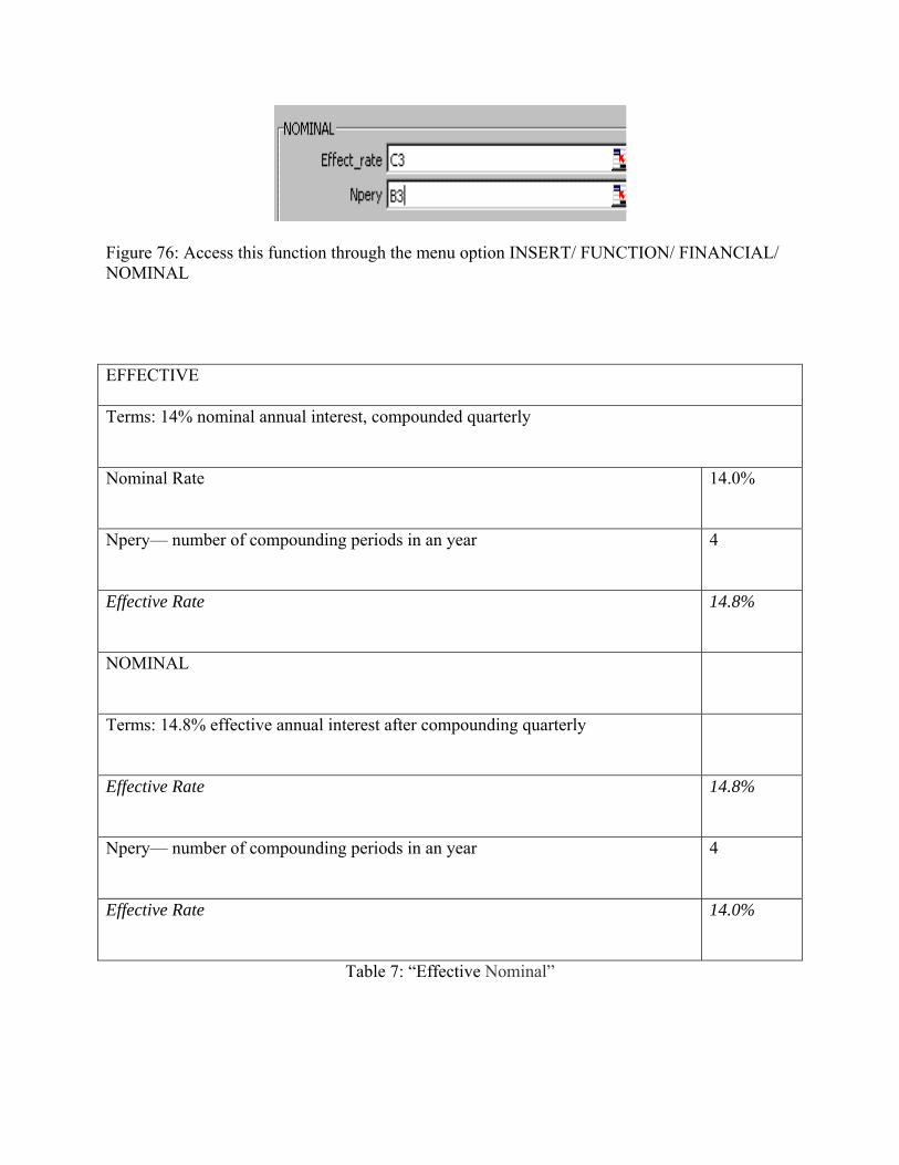
Figure 76: Access this function through the menu option INSERT/ FUNCTION/ FINANCIAL/ NOMINAL EFFECTIVE Terms: 14% nominal annual interest, compounded quarterly Nominal Rate
14.0%
Npery— number of compounding periods in an year
4
Effective Rate
14.8%
NOMINAL
Terms: 14.8% effective annual interest after compounding quarterly
Effective Rate
14.8%
Npery— number of compounding periods in an year
4
Effective Rate
14.0%
Table 7: “Effective Nominal”
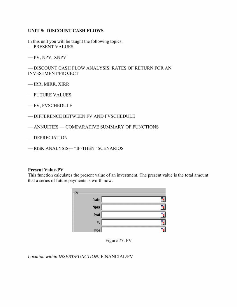
UNIT 5: DISCOUNT CASH FLOWS In this unit you will be taught the following topics: — PRESENT VALUES — PV, NPV, XNPV — DISCOUNT CASH FLOW ANALYSIS: RATES OF RETURN FOR AN INVESTMENT/PROJECT — IRR, MIRR, XIRR — FUTURE VALUES — FV, FVSCHEDULE — DIFFERENCE BETWEEN FV AND FVSCHEDULE — ANNUITIES — COMPARATIVE SUMMARY OF FUNCTIONS — DEPRECIATION — RISK ANALYSIS— “IF-THEN” SCENARIOS Present Value-PV This function calculates the present value of an investment. The present value is the total amount that a series of future payments is worth now.
Figure 77: PV Location within INSERT/FUNCTION: FINANCIAL/PV
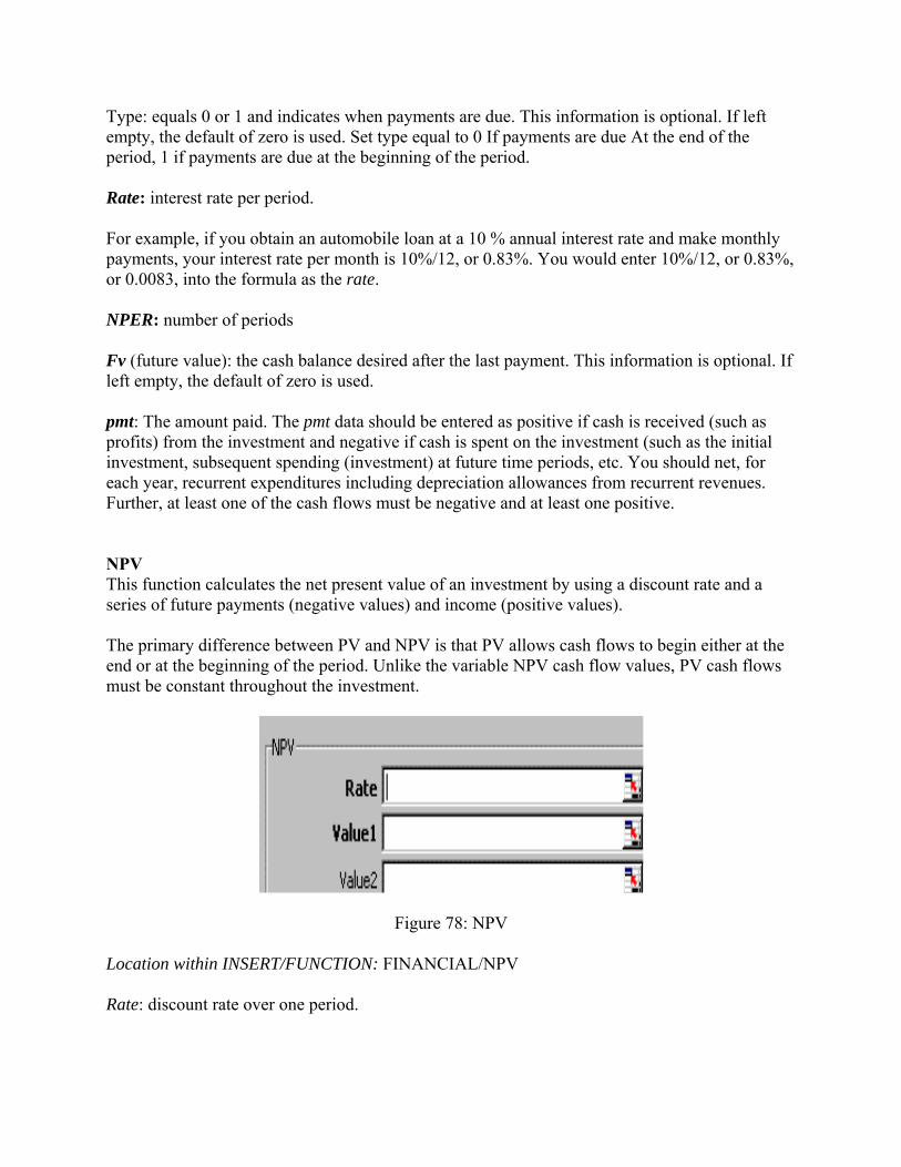
Type: equals 0 or 1 and indicates when payments are due. This information is optional. If left empty, the default of zero is used. Set type equal to 0 If payments are due At the end of the period, 1 if payments are due at the beginning of the period. Rate: interest rate per period. For example, if you obtain an automobile loan at a 10 % annual interest rate and make monthly payments, your interest rate per month is 10%/12, or 0.83%. You would enter 10%/12, or 0.83%, or 0.0083, into the formula as the rate. NPER: number of periods Fv (future value): the cash balance desired after the last payment. This information is optional. If left empty, the default of zero is used. pmt: The amount paid. The pmt data should be entered as positive if cash is received (such as profits) from the investment and negative if cash is spent on the investment (such as the initial investment, subsequent spending (investment) at future time periods, etc. You should net, for each year, recurrent expenditures including depreciation allowances from recurrent revenues. Further, at least one of the cash flows must be negative and at least one positive. NPV This function calculates the net present value of an investment by using a discount rate and a series of future payments (negative values) and income (positive values). The primary difference between PV and NPV is that PV allows cash flows to begin either at the end or at the beginning of the period. Unlike the variable NPV cash flow values, PV cash flows must be constant throughout the investment.
Figure 78: NPV
Location within INSERT/FUNCTION: FINANCIAL/NPV Rate: discount rate over one period.
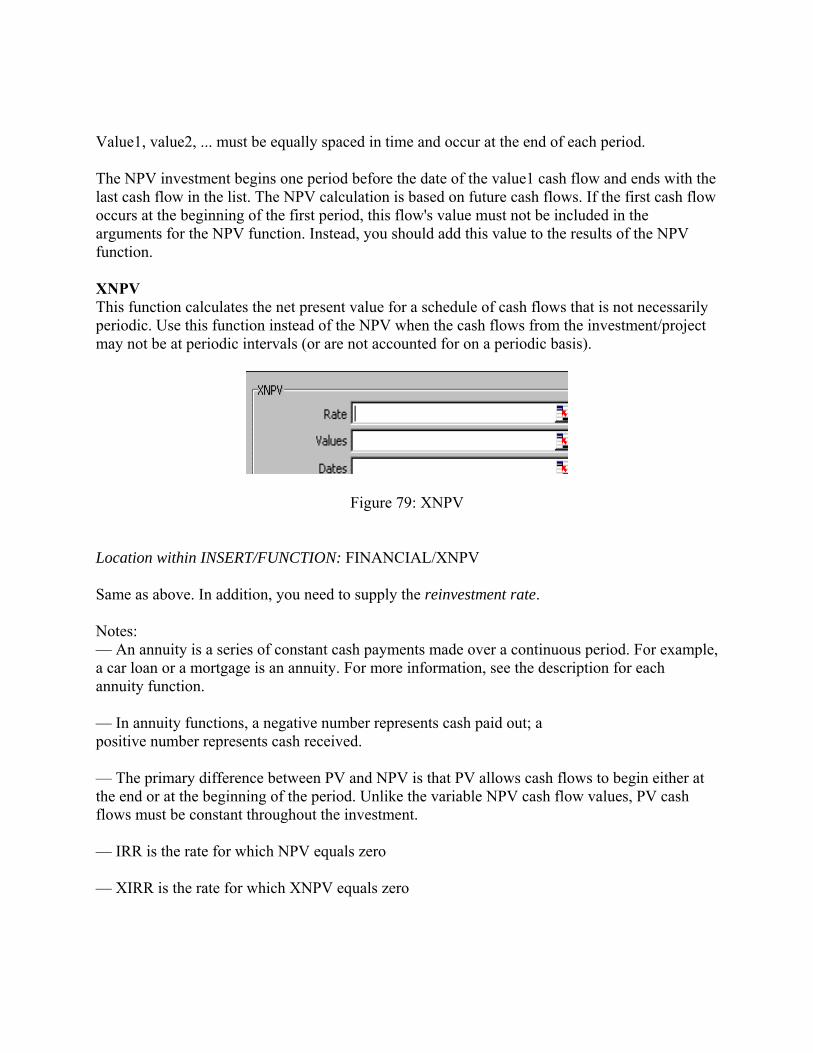
Value1, value2, ... must be equally spaced in time and occur at the end of each period. The NPV investment begins one period before the date of the value1 cash flow and ends with the last cash flow in the list. The NPV calculation is based on future cash flows. If the first cash flow occurs at the beginning of the first period, this flow's value must not be included in the arguments for the NPV function. Instead, you should add this value to the results of the NPV function. XNPV This function calculates the net present value for a schedule of cash flows that is not necessarily periodic. Use this function instead of the NPV when the cash flows from the investment/project may not be at periodic intervals (or are not accounted for on a periodic basis).
Figure 79: XNPV Location within INSERT/FUNCTION: FINANCIAL/XNPV Same as above. In addition, you need to supply the reinvestment rate. Notes: — An annuity is a series of constant cash payments made over a continuous period. For example, a car loan or a mortgage is an annuity. For more information, see the description for each annuity function. — In annuity functions, a negative number represents cash paid out; a positive number represents cash received. — The primary difference between PV and NPV is that PV allows cash flows to begin either at the end or at the beginning of the period. Unlike the variable NPV cash flow values, PV cash flows must be constant throughout the investment. — IRR is the rate for which NPV equals zero — XIRR is the rate for which XNPV equals zero
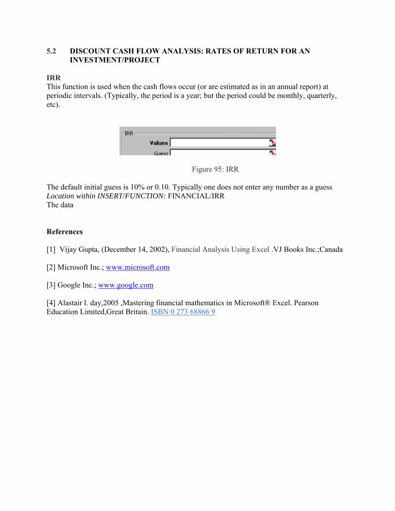
5.2 DISCOUNT CASH FLOW ANALYSIS: RATES OF RETURN FOR AN INVESTMENT/PROJECT
IRR This function is used when the cash flows occur (or are estimated as in an annual report) at periodic intervals. (Typically, the period is a year; but the period could be monthly, quarterly, etc).
Figure 95: IRR The default initial guess is 10% or 0.10. Typically one does not enter any number as a guess Location within INSERT/FUNCTION: FINANCIAL/IRR The data References [1] Vijay Gupta, (December 14, 2002), Financial Analysis Using Excel .VJ Books Inc.;Canada [2] Microsoft Inc.; www.microsoft.com [3] Google Inc.; www.google.com [4] Alastair l. day,2005 ,Mastering financial mathematics in Microsoft® Excel. Pearson Education Limited,Great Britain. ISBN 0 273 68866 9