Embed Size (px)
Citation preview

CENTRE FOR APPLIED MACROECONOMIC ANALYSIS
The Australian National University
________________________________________________________________ CAMA Working Paper Series April, 2010 ________________________________________________________________
FORECAST DENSITIES FOR ECONOMIC AGGREGATES FROM DISAGGREGATE ENSEMBLES Francesco Ravazzolo Norges Bank Shaun P. Vahey The Australian National University ___________________________________________________________________________
CAMA Working Paper 10/2010 http://cama.anu.edu.au

Forecast Densities for Economic Aggregates fromDisaggregate Ensembles∗
Francesco Ravazzolo†
(Norges Bank)Shaun P. Vahey‡
(ANU)
March 12, 2010
Abstract
We propose a methodology for producing forecast densities for economic ag-gregates based on disaggregate evidence. Our ensemble predictive methodologyutilizes a linear mixture of experts framework to combine the forecast densitiesfrom potentially many component models. Each component represents the uni-variate dynamic process followed by a single disaggregate variable. The ensembleproduced from these components approximates the many unknown relationshipsbetween the disaggregates and the aggregate by using time-varying weights on thecomponent forecast densities. In our application, we use the disaggregate ensembleapproach to forecast US Personal Consumption Expenditure inflation from 1997Q2to 2008Q1. Our ensemble combining the evidence from 11 disaggregate series out-performs an aggregate autoregressive benchmark, and an aggregate time-varyingparameter specification in density forecasting.
Keywords: Ensemble forecasting, disaggregatesJEL codes: C11; C32; C53; E37; E52
∗We benefited greatly from discussions with Todd Clark, Anthony Garratt, Kirstin Hubrich, ChristianKascha, James Mitchell, Tara Sinclair and Michael Smith. We thank conference and seminar participantsat Oslo University, the European Central Bank, the Veissmann European Research Centre, and theSociety for Nonlinear Dynamics and Econometrics 17th Annual Symposium. The views expressed in thispaper are our own and do not necessarily reflect those of Norges Bank. We thank the ARC (LP 0991098)for support.
†Norges Bank, Research Department. [email protected]‡Corresponding author : Shaun Vahey, CAMA, ANU. [email protected]
1

1 Introduction
Policymakers regularly combine the leading evidence in disaggregate series to carry out
probabilistic assessments of aggregate behavior; see, for example, Greenspan (2004), and
the discussions by Feinstein, King, and Yellen (2004). To our knowledge, economists have
not explored formally the scope for producing density forecasts for economic aggregates
based on disaggregate information. This is surprising given the widespread recognition
that evaluations of point forecast accuracy are only relevant for highly restricted loss
functions. More generally, complete probability distributions over outcomes provide in-
formation which is helpful for making economic decisions; see, for example, Granger and
Pesaran (2000) and Timmermann (2006). Accordingly, several central banks, including
the US Federal Reserve, have committed to density or interval forecasts in recent years.
In this paper, we propose an ensemble methodology for combining the evidence in dis-
aggregate series to make probabilistic forecasts for an economic aggregate. We formulate
the forecasting problem as one in which a forecaster (recursively) selects a linear combi-
nation of component forecast densities to produce an ensemble forecast density for the
aggregate. Each component forecast is produced from a univariate time series model for a
single disaggregate series. The resulting ensemble approximates the many unknown rela-
tionships between the disaggregates and the aggregate using time-varying weights across
the disaggregate forecast densities. Construction of the disaggregate ensemble forecast for
the economic aggregate uses out of sample density combination methods; see, for example,
Jore, Mitchell and Vahey (2010).
In our application based on US Personal Consumption Expenditure deflator data, we
assess the forecast performance of the disaggregate ensemble approach over the out of
sample period 1997Q2 to 2008Q1. An ensemble combining the evidence from 11 disag-
gregate series outperforms an aggregate autoregressive benchmark, and also an aggregate
time-varying parameter specification in density forecasting. Our applied macroeconomic
work extends the case for forecast combinations, made by (among others) Stock and Wat-
son (2003) and Clark and McCracken (2010), to forecast densities for economic aggregates
2

from disaggregate information.
The remainder of this paper is structured as follows. In Section 2, we describe our
methods for ensemble modeling of the relationship between the economic aggregate and
the disaggregates. In Section 3, we apply our methodology to US data to produce ag-
gregate inflation forecast densities from an ensemble system utilizing disaggregate infor-
mation. We compare and contrast the ensemble predictive densities with those resulting
from our alternative specifications which ignore disaggregate information. In the final
section, we conclude.
2 Disaggregate Ensemble Forecast Methodology
The theoretical insights of Bates and Granger (1969) and the macroeconomic forecast eval-
uation studies by (among others) Stock and Watson (2003) and Clark and McCracken
(2010) suggest that forecast combination can be an effective tool for point forecasting.
Jore, Mitchell and Vahey (2010) and Garratt, Mitchell and Vahey (2009) establish the
performance credentials of forecast combinations for macroeconomic aggregates using en-
sembles of vector autoregression (VAR) components.
Outside of the economics literature, meteorologists commonly construct ensemble den-
sities to deal with model and/or measurement uncertainty. For an early description of
a weather ensemble forecasting see Molteni et al (1996), and more recent contributions
in this field by Raftery et al (2005), and Bao et al (2010). Murphy et al (2004) discuss
ensembles for modeling climate change; Lopez et al (2009) examine the impact of climate
change on resources.
The methodology proposed in this paper extends the scope of the ensemble macroeco-
nomic forecasting framework, developed by Jore, Mitchell and Vahey (2010) and Garratt,
Mitchell and Vahey (2009), to disaggregate systems. These existing macroeconomic fore-
casting exercises consider combinations of forecast densities from models with a small
number of (three, or less) candidate variables. With a large number of (lagged) disag-
gregate variables which could be used to forecast an economic aggregate, the applied re-
3

searcher faces a severe computational difficulty. For example, given 10 disaggregates, and
restricting attention to a single lag of each disaggregate, the researcher faces 210 = 1024
feasible forecasting specifications for the aggregate. Allowing for anything beyond first-
order dynamics is prohibitively burdensome computationally. For example, just one or
two lags of each disaggregate variable would give 220 = 1, 048, 576 variants. And of
course, whatever model selection methodology is applied by the researcher, there will be
considerable model uncertainty about which specification is ‘best’ in practice.
In this paper, we overcome the curse of dimensionality resulting from forecasting with
disaggregates by approximating the interactions between the many disaggregates and the
aggregate. Each component in the ensemble represents the dynamic univariate time series
process for a single disaggregate variable. Then we take time-varying weighted combina-
tions of the forecast densities produced from the individual components to construct the
ensemble predictive density for the aggregate. The calibration properties of the ensemble
forecast densities provides guidance on the appropriateness of the approximation. Bache
et al (2009) and Geweke (2009) discuss the interpretation of forecast density combinations
in the presence of an incomplete model space.
2.1 Disaggregate Ensemble Construction
We consider a forecaster combining out of sample forecast densities provided by compo-
nent models. Timmermann (2006, p177) discusses out of sample density combination.
Recent applications include Wallis (2005), aggregating survey information, and Mitchell
and Hall (2005), combining forecasts from two institutions.
We assume that the forecaster has uninformative priors over the forecast densities pro-
duced by the component models. In principle, off-model information—such as assigning
prior mass to the expenditure shares used to define the aggregate index—could be helpful
in forecasting applications. However, a prior elicitation problem arises with dynamic in-
terrelationships between (potentially, a large number of) disaggregates. Hence, we leave
an investigation of the scope for informative component priors to subsequent research.
4

Given i = 1, . . . , N disaggregates (where N could be a large number), we define the
disaggregate ensemble (DE) by the convex combination sometimes referred to as a linear
opinion pool. The disaggregate ensemble is defined as:
DE = g(Yτ ) =N
i=1
wi,τ h(Yτ | Ii,τ ), τ = τ , . . . , τ , (1)
where h(Yτ | Ii,τ ) are the one step ahead forecast densities from component model i,
i = 1, . . . , N of the economic aggregate Yτ , conditional on the information set Ii,τ .
Each component produces one step ahead forecasts for the aggregate. Hence, the
variables used to produce a one step ahead forecast density for τ are dated τ − 1 or
earlier. Although we do not explore this issue here, a density combination framework can
easily be extended to forecast horizons greater than one; see, for example, Jore, Mitchell
and Vahey (2010). The non-negative weights, wi,τ , in this finite mixture sum to unity,
are positive, and vary by recursion in the evaluation period τ = τ , . . . , τ .
Notice that our ensemble framework does not restrict the way in which the compo-
nent forecasts are produced. The component models could have time-varying or con-
stant parameters. The members of the ensemble could be estimated by frequentist or
Bayesian methods, with or without the aid of conventional regression diagnostics. And
the component models need not utilize the same in-sample observations for parameter
estimation—rolling regression variants can be accommodated in the out of sample den-
sity combination exercise. Notice also that the disaggregate ensemble will be a mixture of
the forecast densities produced by the components. Hence, the ensemble given by equa-
tion (1) can accommodate non-Gaussian predictive densities. This flexibility can be very
useful in adapting the methodology to applied economic issues. Kascha and Ravazzolo
(2010) discuss the methods to restrict the ensemble densities to be both unimodal and
symmetric if required.
5

2.2 Component Model Space
Macroeconomic disaggregate time series variables commonly exhibit parameter change,
and applied researchers often utilize Bayesian methods to accommodate this feature. With
this in mind, consider a mixture innovation model for a single disaggregate variable, π:
πt = β0t +k
p=1 βptπt−p + σtεt
βjt = βj,t−1 + κjtηjt, j = 0, . . . , k
lnσ2t = lnσ2
t−1 + κk+1,tηk+1,t
(2)
where t = 1, ..., τ − 1, εt ∼ N(0, 1), ηt = (η0t, ..., ηk+1,t) ∼ N(0, Q) with Q a diagonal
matrix and elements q20, . . . , q2k+1, and κt = (κ0t, . . . ,κk+1,t) is a ((k + 2) × 1) vector of
unobserved uncorrelated 0/1 processes with Pr[κjt = 1] = pj for j = 0, . . . , k + 1.
Hence, each of the regression parameters βjt and the residual variance σ2t remain the
same as their previous values βj,t−1 and σ2t−1 unless κjt = 1 and κk+1,t = 1 in which case
βjt changes with ηjt and ln(σt)2 changes with ηk+1,t respectively. See, for example, Koop
and Potter (2007) and Giordani, Kohn, van Dijk (2007) for similar approaches. As the
changes in the variance parameters lnσ2t are stochastic we allow for a form of stochastic
volatility; see Giordani and Kohn (2008). The flexibility of the specification in (2) stems
from the fact that the parameters βt = (β0t, . . . , βkt) and σ2t are allowed to change every
time period, but they need not change. The occurrence of a change is described by the
latent binary random variable κjt, while the magnitude of the change is determined by ηjt,
which is assumed to be normally distributed with mean zero. An attractive property of (2)
is that the changes in the individual regression parameters are not restricted to coincide
but rather are allowed to occur at different points in time. Given the popularity of this
specification for modeling time variation in autoregressions, we relegate our discussion of
the computational steps to Appendix A.1. We describe the disaggregate forecast densities
from equation (2) in Appendix A.2.
We emphasize that the component specification described by equation (2) repre-
6

sents an autoregressive forecasting relationship (with parameter change) for a single
disaggregate—the aggregate variable of interest does not enter equation (2). In applied
ensemble work, the component (in our case, disaggregate) model forecasts might be badly
behaved. The forecast densities from a given component could be too diffuse, or too
narrow, and/or the forecasts might exhibit individual bias. It is common in the ensemble
literature to consider adjusting the spread and/or the central location of each compo-
nent density prior to combination; see, the discussions in (among others) Atger (2003),
Stensrud and Yussouff (2007) and Bao et al (2010). In our disaggregate forecasting exer-
cise, the disaggregate forecast, πτ , may not be an efficient forecast of the aggregate, Yτ .
Although more flexible approaches are feasible, a simple bias-correction step to the com-
ponent forecasts has often been found to be sufficient to ensure well-calibrated ensemble
densities in practice; see, for example, Stensrud and Youssoff (2007). To implement this
post-processing step, estimate with (recursive) Ordinary Least Squares (OLS):
Ys = a+ pe(πs | Ii,s) + εs, s = s, . . . , τ − 1 (3)
where pe(πs|Ii,s) is the expected value (for example, the median) of the predictive den-
sity p(πs | Ii,s) from the ith disaggregate component. Then, define the bias-corrected
disaggregate forecast density for the aggregate:
h(Yτ | Ii,τ ) = p(πτ | Ii,τ ) + a (4)
where a is the OLS estimate of a in (3). The bias-corrected disaggregate forecast density
h(Yτ | Ii,τ ) is used to construct the ensemble forecast density for the aggregate, g(Yτ ).
We note that although we consider a time-varying parameter model for the disaggre-
gate time series, this is not a necessary feature of the ensemble approach. For example,
Ravazzolo and Vahey (2009) utilize (recursively-estimated) constant parameter autore-
gressive components to forecast inflation in Australia.
7

2.3 Disaggregate Ensemble Weights
We complete our description of the disaggregate ensemble prediction system by specifying
the construction of the time-varying weights. A number of studies in the economics
literature have used density scoring rules. Mitchell and Wallis (2010) provide a recent
discussion of scoring rules and the justification for testing relative density forecasting
performance from the perspective of the Kullback-Leibler Information Criterion (KLIC).
Gneiting and Raftery (2007) analyze the relationships between scoring rules and Bayes
factors. Corradi and Swanson (2006) provide an extensive review of measures of density
forecast performance.
Outside the econometrics literature, Hersbach (2000), Gneiting and Raftery (2007)
and Panagiotelis and Smith (2008) have argued that the Continuous Ranked Probability
Score (CRPS), which rewards predictive densities with high probabilities near (and at)
the outturn, provides a robust metric of density forecast performance. Gneiting and
Raftery (2007) refer to the concentration of a forecast density about its central location
as ‘sharpness’, and the location as ‘distance’. The CRPS metric favors densities with
small distance and high sharpness.
The CRPS is measured as the difference between the predicted and actual cumulative
distribution. Figure 1 provides an illustrative example for a particular observation: the
CRPS measures the area between the predictive (for this example, assumed to be Gaus-
sian) and the actual cumulative distribution (marked by shading). The (positive) score
approaches zero as the predictive density converges on the true (but unobserved) density.
More formally, following Panagiotelis and Smith (2008), the CRPS of a component
density for a particular observation can be defined as:
CRPS = Eh|y − Y |− 0.5Eh|y − y| (5)
where Eh is the expectation for the predictive h(Yτ ), y and y are independent random
draws from the predictive, and Y is the observed outturn. The expectation terms can
be approximated using the Monte Carlo draws from the component forecast density;
Panagiotelis and Smith (2008, equation 4.5) provide the computational steps required.
8

For each bias-corrected disaggregate forecast density, we construct the mean CRPS
averaged over the evaluation period. The weight on an individual component density i in
each observation of the evaluation period is then calculated by:
wi,τ =
τ−1s X(h(Yτ | Ii,τ ))
Ni=1
τ−1s X(h(Yτ | Ii,τ ))
, τ = s, . . . , τ , . . . , τ . (6)
with X is the inverse of the mean CRPS, 0 ≤ X ≤ ∞, and higher scores are preferred.
2.4 Methodological Summary
Our disaggregate ensemble methodology can be summarized as follows. For each obser-
vation in the forecaster’s evaluation period, we estimate N univariate time series repre-
sentations, one for each disaggregate. The ‘fit’ of each bias-corrected component forecast
density is assessed with the CRPS, and used to construct weights for the ensemble fore-
cast density. These weights vary through the evaluation period. In this manner, we
approximate the forecast densities for the true, but unknown, relationships between the
disaggregates and the aggregate. The appropriateness of the approximation can be as-
sessed by examining the calibration properties of the ensemble forecast densities. (We
shall utilize a number of well-known calibration tests in the subsequent application.)
3 Application: forecasting inflation for the US
In this forecasting US inflation application, we consider US Personal Consumption Ex-
penditure deflator (PCE) data. We construct a disaggregate ensemble using an evaluation
period from 1997Q2 to 2008Q1, and then examine the calibration of the ensemble aggre-
gate inflation forecast densities using probability integral transforms, PITS, at the end of
the evaluation. We also examine forecast performance relative to a number of aggregate
benchmarks. We stress that our focus in this example is the predictive performance of the
ensemble. We do not aim to select a preferred single disaggregate predictor of aggregate
inflation from the (likely) misspecified disaggregate components.
9

We begin our analysis by describing the US data. Then we describe our disaggregates
ensemble, aggregate benchmarks, density evaluation methods, and results.
3.1 Data
The dataset contains time series for the disaggregate components of the PCE. The data
are available on the Bureau of Economic analysis http://www.bea.gov/national/nipaweb.
To our knowledge, the disaggregate data used in this study are not available on a real-time
basis, although Croushore (2009) discusses the revisions in aggregate PCE. The PCE data
permit breakdowns at various levels of disaggregation. Tables AI-AIII in Clark (2006)
provide further details on levels of disaggregation in the US PCE data.
We emphasize that, in principle, our methodology could be applied to any level of
disaggregation. In our application, we illustrate our technique with 11 disaggregates.
These are Motor Vehicles, Household Equipment, Other Durables, Clothing, Other Non-
durables, Housing, Household Operation, Transport, Medical Care, Recreation and Other
Services. For all inflation series, PCE and its disaggregates, we work with the quarterly
growth rates (calculated as 100 time the log difference in the price levels) plotted in fig-
ure 2. The volatility and the mean of PCE measured inflation vary through the sample
as figure 2 makes clear, providing some motivation for time-varying parameter specifica-
tions. The 11 disaggregate series display varying degrees of shifting levels and changes
in volatility: Motor Vehicles, Household Equipment, Other Durables, and Other Non-
durables have marked changes in levels; Household Operation, Transport, Recreation and
Other Services show signs of volatility changes; and Clothing, Housing, and Medical Care
exhibit both characteristics relatively strongly. Overall, the data display considerable
time variation and heterogeneity across disaggregates.
Using conventional assumptions about the timing of Great Moderation, we start our
sample for component estimation with 1984Q1 and end with 2008Q1. Hence, we restrict
our analysis to the period in which conventional wisdom has it that inflation is diffi-
cult to predict in terms of point forecast accuracy; see, for example, Stock and Watson
10
(2007). With our evaluation period (τ) from 1997Q2 (τ) to 2008Q1 (τ), the period 1993Q2
to 1997Q1 comprises a ‘training period’ to initialize the ensemble weights. The bias-
correction step is based on a rolling window of 20 quarters, denoted s = τ − 20, . . . , τ − 1,
for the results reported below. (Using the training period plus the evaluation period
for bias-correction gave some degradation in relative performance but the disaggregate
ensemble always outperformed the aggregate benchmark.)
3.2 Disaggregate Ensemble and Aggregate Benchmarks
The ensemble forecast densities for aggregate inflation use equations (1)-(6) described
above. In addition to our disaggregate ensemble, DE11, we also evaluate the predictive
densities from two time series models of aggregate inflation. The first uses a linear model
to forecast measured inflation without disaggregate information. That is, using a linear
autoregressive model for aggregate measured inflation, with two lags, AR(2). We use
uninformative priors for the AR(2) parameters with an expanding window. The predictive
densities follow the t-distribution, with mean and variance equal to OLS estimates; see,
for example, Koop (2003) for details. We use this AR model as our benchmark in tests
of relative forecast performance.
The second aggregate variant uses a single time-varying parameter autoregressive spec-
ification similar to equation (2), but for aggregate inflation, Yτ , with no disaggregate in-
formation. For both the aggregate and the disaggregate time-varying specifications we
use four autoregressive terms (that is, we set k = 4).
3.3 Density Evaluation
Following (among others) Jore, Mitchell and Vahey (2010), we evaluate the ensemble pre-
dictive densities using a battery of (one-shot) tests of absolute forecast accuracy, relative
to the ‘true’ but unobserved density. Like Rosenblatt (1952) and Diebold, Gunther and
Tay (1998), we utilize the probability integral transforms, PITS, of the realization of the
variable with respect to the forecast densities. A forecast density is preferred if the density
11

is correctly calibrated, regardless of the forecasters loss function. The PITS are:
zτ =
πτ
−∞p(u)du.
The PITS should be both uniformly distributed, and independently and identically dis-
tributed if the forecast densities are correctly calibrated. Hence, calibration evaluation
requires the application of tests for goodness-of-fit and independence. Given the large
number of bias-corrected component forecast densities under consideration in the ensem-
ble, we do not allow for estimation uncertainty in the components when evaluating the
PITS. Corradi and Swanson (2006) review tests computationally feasible for small N .
The goodness-of-fit tests employed include the Likelihood Ratio (LR) test proposed
by Berkowitz (2001), the Anderson-Darling test, and the Pearson (χ2) test used by Wallis
(2003). Our Berkowitz test is a three degrees of freedom variant, with a test for indepen-
dence, where under the alternative zτ follows an AR(1) process. The Anderson-Darling
(AD) test for uniformity, a modification of the Kolmogorov-Smirnov test, gives more
weight to the tails of the forecast density. The Pearson (χ2) tests divides the range of the
zτ into eight equiprobable classes and tests for uniformity in the histogram. We also test
directly for independence of the PITS using a Ljung-Box (LB) test, based on autocor-
relation coefficients up to four. A well-calibrated ensemble should give high probability
values for all four of these tests—implying the null hypothesis of no calibration failure
cannot be rejected.
Turning to our analysis of relative predictive accuracy, we consider a Kullback-Leibler
Information Criterion (KLIC) based test, utilizing the expected difference in the Loga-
rithmic Scores of the candidate forecast densities; see, for example, Bao, Lee and Saltoglu
(2007), Mitchell and Hall (2005) and Amisano and Giacomini (2007). Suppose there
are two density forecasts, g(Yτ | I1,τ ) and g(Yτ | I2,τ ), and consider the loss differ-
ential dτ = ln g(Yτ | I1,τ ) − ln g(Yτ | I2,τ ). The null hypothesis of equal accuracy is
H0 : E(dτ ) = 0. The sample mean, dτ , has under appropriate assumptions the limiting
distribution:√T (dτ − dτ ) → N(0,Ω). The Logarithmic Score of the ith density forecast,
ln g(Yτ | Ii,τ ), is the logarithm of the probability density function g(. | Ii,τ ), evaluated
12

at the outturn Yτ . In our LS test of relative forecast performance, we abstract from the
estimation procedure used to generate the forecast densities. Mitchell and Wallis (2010)
discuss the value of information-based methods for evaluating forecast densities that are
well-calibrated on the basis of PITS tests.
3.4 Results
Before considering the density evaluations for our disaggregate ensemble, we summa-
rize the point forecast performance. Both the disaggregate ensemble (DE11) and the
time-varying parameter aggregate autoregressive model (TVPAR) are considerably out-
performed by the aggregate AR(2) model in terms of root mean squared prediction error
(RMSPE). For the AR(2) benchmark, the raw RMSPE is 0.163. The other specifications
give figures approximately 60 percent higher. Stock and Watson (2007) discuss the dif-
ficulty of outperforming simple benchmarks in terms of RMSPE with Great Moderation
data; see also Groen, Paap and Ravazzolo (2009) for similar results.
The evaluation of the forecast densities are presented in table 1. The three rows refer
to the disaggregate ensemble, DE11, the aggregate autoregressive benchmark, AR(2), and
the aggregate time-varying parameter model, TVPAR, respectively. The five columns of
table 1 report the p-values for the Berkowitz LR test, the Anderson-Darling AD test, the
χ2, the LB test, and the Logarithmic Scores (averaged over the evaluation period).
Looking at the DE11 results shown in the top row, we see that the null hypothesis
of no calibration failure cannot be rejected at the 1 percent significance level for all of
the four individual diagnostic tests, marked in bold. (Using a 5 percent significance level,
the χ2 test is (just) failed with a 4.8 percent probability value.) We note that each of
these diagnostic tests for calibration is conducted on an individual basis. A 5 percent
significance level on each individual test would imply a Bonferroni-corrected p-value of
5/4=1.25 percent (reported as 0.0125 in the table).
The aggregate specifications, shown in the remaining two rows of table 1, display a
number of instances of calibration failure. The AR(2) benchmark, first row, fails all of
13

the diagnostic tests, with three p-values below 1 percent. The more flexible aggregate
specification, TVPAR, fails two of the four tests at the 1 percent level. Namely, the LR
and the χ2.
Figure 3 plots the PITS histograms for the three candidates, the DE11, the AR(2)
and the TVPAR. The histogram for the AR(2) displays severe departures from uniformity.
The TVPAR and DE11 are more evenly spread across the decile counts, although visual
inspection suggests calibration could be improved in both cases.
Turning to the Logarithmic Scores of the forecast densities, shown in the fifth column of
table 1, we see that the disaggregate ensemble DE11 records the best relative performance,
roughly 26 percent of the AR(2). The LS test p-value (marked in bold) indicates that the
null hypothesis of equal forecast performance can be rejected at the 1 percent significance
level. The time-varying parameter aggregate specification also improves on the the AR(2)
benchmark, at roughly 60 percent. An LS test of the DE11 relative to the TVPAR
confirms the superiority of the DE11 at the 1 percent significance level.
To shed further light on the contribution of disaggregate information, figure 4 plots
the weights in the disaggregate ensemble DE11. As we might expect, given the univariate
nature of the components, there is uncertainty about the relative importance of disaggre-
gate components through the evaluation. The weights lie in the (approximate) interval
[0.04, 0.18] at the beginning of the evaluation. But the dispersion in the weights drops as
the top three disaggregates decline in importance through the evaluation.
In figure 5, we plot the median from our disaggregate ensemble, together with ag-
gregate PCE inflation. The 25th and 75th percentiles from the ensemble density are also
shown. The plot shows that the median of the DE11 is considerably less volatile than
the actual aggregate inflation series. The central mass of the predictive density is around
0.3 percent prior to 2004, and slightly higher thereafter. The difference between the two
percentiles shown varies very little through the evaluation, typically remaining close to
0.4 percentage points. We note that the number of inflation outturns above the 75th per-
centile is somewhat larger than the number below the 25thpercentile. Although the PITS
tests indicate that the ensemble forecast densities are correctly calibrated, clearly there
14

is scope for further improvement.
We draw the following conclusions from our forecast density evaluations. First, the
disaggregate ensemble DE11 performs well in both tests of absolute and relative density
forecasting performance. Second, as Jore, Mitchell and Vahey (2010) and Clark (2009)
emphasize, although simple autoregressive models of aggregate inflation produce accurate
point forecasts, the benchmark can be bettered in terms of forecast densities.
4 Conclusions
In this paper, we have proposed a methodology for constructing forecast densities for
economic aggregates based on disaggregate evidence using an ensemble predictive system.
In our application, we have shown that the disaggregate ensemble approach delivers well-
calibrated forecast densities for US PCE aggregate inflation from 1997Q2 to 2008Q1.
Alternative forecasting specifications for the aggregate based on time-varying models or
simple autoregressive benchmarks failed to match the density forecasting performance of
our disaggregate ensemble.
Our applied work indicates that including disaggregate information via an ensemble
system improves probabilistic forecasts for US aggregate inflation. This result mirrors
similar findings in other fields where ensemble methods have been widely adopted by
practitioners to provide a pragmatic framework for probabilistic assessment. Our results
also confirm formally the view endorsed by many economic policymakers that disaggregate
information can be helpful for forecasting.
15
5 References
Altger, F. (2003) “Spatial and interannual variability of the reliability of ensemble-
based probabilistic forecasts: Consequences for calibration”, Monthly Weather Review,
131, 1509-1523.
Amisano, G. and R. Giacomini (2007), “Comparing Density Forecasts via Likelihood
Ratio Tests”, Journal of Business and Economic Statistics, 25, 2, 177-190.
Bache, I.W., J. Mitchell, F. Ravazzolo and S.P. Vahey (2009) “Macro modeling with
many models”, Norges Bank Working Paper, 2009/15.
Bao, Y., T-H. Lee and B. Saltoglu (2007), “Comparing Density Forecast Models”,
Journal of Forecasting, 26, 203-225.
Bao, L., T. Gneiting, E.P. Grimit, P. Guttop, and A.E. Raftery (2010), “Bias Correc-
tion and Bayesian Model Averaging for Ensemble Forecasts of Surface Wind Direction”,
Monthly Weather Review, forthcoming.
Bates, J.M. and C.W.J. Granger (1969), “Combination of Forecasts”, Operational
Research Quarterly, 20, 451-468.
Berkowitz, J. (2001) “Testing density forecasts, with applications to risk manage-
ment”, Journal of Business and Economic Statistics, 19, 465-474.
Carter, C. and R. Kohn (1994) “On Gibbs sampling for state-space models”, Biometrika,
81, 541-553.
Carter, C. and R. Kohn (1997) “Semiparametric Bayesian inference for time series
with mixed spectra”, Journal of the Royal Statistical Society, Series B, 255-268.
Clark, T.E. (2006) “Disaggregate evidence on the persistence of consumer price infla-
tion, Journal of Applied Econometrics, 21, 563-587.
Clark, T.E. (2009) “Real-time density forecasts from VARs with stochastic volatility”,
FRB Kansas City Working Paper, RWP 09-08.
Clark T.E. and M.W. McCracken (2010) “Averaging forecasts from VARs with uncer-
tain instabilities”, Journal of Applied Econometrics, 25, 5-29.
16

Corradi, V., and N.R. Swanson (2006) “Predictive density evaluation”, in G. Elliot, C.
W. J. Granger, and A. Timmermann(eds.) Handbook of Economic Forecasting, Elsevier,
197 - 284.
Croushore, D. (2009) “Revisions to PCE inflation measures: implications for monetary
policy”, FRB Philadelphia Working Paper 08-8, revised July 2009.
Diebold, F.X., T.A. Gunther, and A.S. Tay (1998) “Evaluating density forecasts; with
applications to financial risk management”, International Economic Review, 39, 863-83.
Feinstein, M., M.A. King, and J. Yellen (2004) “Innovations and issues in monetary
policy: panel discussion”, American Economic Review, Papers and Proceedings, May,
41-48.
Garratt, A., J. Mitchell and S.P. Vahey (2009) “Measuring output gap uncertainty”,
Reserve Bank of New Zealand Discussion Paper, DP 2009/15.
Geman, S. and D. Geman (1984) “Stochastic relaxation, Gibbs distributions and the
Bayesian restoration of images”, IEEE Transaction on Pattern Analysis and Machine
Intelligence, 6, 721-741.
Gerlach, R., C. Carter, and R. Kohn (2000) “Efficient Bayesian inference for dynamic
mixture models”, Journal of the American Statistical Association, 95, 819-828.
Geweke, J. (2009) “Complete and Incomplete Econometric Models”, Princeton Uni-
versity Press.
Giordani, P. and R. Kohn (2008) “Efficient Bayesian inference for multiple change-
point and mixture innovation models”, Journal of Business and Economic Statistics, 26,
66-77.
Giordani, P., R. Kohn, and D. van Dijk (2007) “A united approach to nonlinearity,
outliers and structural breaks”, Journal of Econometrics, 137, 112-137.
Gneiting, T. and A.E. Raftery (2007) “Strictly proper scoring rules, prediction and
estimation”, Journal of the American Statistical Society, 102, 477, 359-378.
Granger, C. and M.H. Pesaran (2000) Economic and statistical measures of forecast
accuracy, Journal of Forecasting, 19, 537-560.
Greenspan, A. (2004) “Risk and uncertainty in monetary policy”, American Economic
17

Review, Papers and Proceedings, May, 33-40.
Groen, J.J.J., R. Paap and F. Ravazzolo (2009) “Real-time inflation forecasting in a
changing world”, Norges Bank Working Paper, 2009/16.
Hersbach, H. (2000) “Decomposition of the continuous ranked probability score for
ensemble prediction systems”, Weather and Forecasting, 15, 559-570.
Jore, A.S., J. Mitchell and S.P. Vahey (2010)“Combining forecast densities from VARs
with uncertain instabilities”, Journal of Applied Econometrics, forthcoming.
Kascha, C. and F. Ravazzolo (2010) “Combining inflation density forecasts”, Journal
of Forecasting, 29, 231-250.
Kim, S., S. Shephard, and S. Chib (1998) “Stochastic volatility: Likelihood inference
and comparison with ARCH models, Review of Economic Studies, 65, 361-393.
Koop, G. (2003) Bayesian Econometrics, Wiley.
Koop, G. and S. Potter (2007) “Estimation and forecasting in models with multiple
breaks”, Review of Economic Studies, 2007, 74, 763-789.
Lopez, A., F. Fung, M. New, G. Watts, A. Weston, R.L. Wilby (2009) “From climate
model ensembles to climate change impacts and adaptation: A case study of water re-
source management in the southwest of England”,Water Resources Research, 45, W08419,
1-21.
Mitchell, J. and S.G. Hall (2005) “Evaluating, comparing and combining density fore-
casts using the KLIC with an application to the Bank of England and NIESR fan charts
of inflation”, Oxford Bulletin of Economics and Statistics, 67, 995-1033.
Mitchell, J. and K.F. Wallis (2010) “Evaluating density forecasts: Forecast combi-
nations, model mixtures, calibration and sharpness”, Journal of Applied Econometrics,
forthcoming.
Molteni, F., R. Buizza, T.N. Palmer and T. Petroliagis (1996) “The new ECMWF
ensemble prediction system: methodology and validation”, Quarterly Journal of the Royal
Meteorological Society, 122, 73-119.
Murphy, J.M., D.M.H. Sexton, D.N. Barnett, G.S. Jones, M.J. Webb, M. Collins and
D.A. Stainforth (2004) “Quantification of modelling uncertainties in large ensembles of
18

climate change simulations”, Nature, 430, 768-772.
Panagiotelis, A. and M. Smith (2008) “Bayesian density forecasting if intraday elec-
tricity prices using multivariate skew t distribution”, International Journal of Forecasting,
24, 710-727.
Raftery, A.E., T. Gneiting, F. Balabdaoui and M. Polakowski, (2005) “Using Bayesian
model averaging to calibrate forecast ensembles”, Monthly Weather Review, 133, 1155-
1174.
Ravazzolo, F. and S.P. Vahey (2009) “Measuring core inflation in Australia with disag-
gregate ensembles”, available from http://www.rba.gov.au/publications/confs/2009/index.html.
Rosenblatt, M. (1952) “Remarks on a multivariate transformation”, The Annals of
Mathematical Statistics, 23, 470-472.
Shephard, N. (1994), “Partial non-Gaussian state-space models”, Biometrika, 81, 115-
131.
Stensrud, D.J. and N. Yussouf (2007) “Bias-corrected short-range ensemble forecasts
of near surface variables”, Meteorological Applications, 12, 217-230.
Stock, J.H. and M.W. Watson (2003) “Forecasting output and inflation: The role of
asset prices”, Journal of Economic Literature, 41, 788-829.
Stock, J.H. and M.W. Watson (2007) “Why has US inflation become harder to fore-
cast?”, Journal of Money, Credit and Banking, 39, 3-34.
Tanner, M. and W. Wong (1987) “The calculation of posterior distributions by data
augmentation, Journal of the American Statistical Association, 82, 528-550.
Timmermann, A. (2006) “Forecast combination”, G. Elliot, C. Granger, C. and A.
Timmermann (eds.) Handbook of Economic Forecasting, North-Holland, 197-284.
Wallis, K.F. (2003) “Chi-squared tests of interval and density forecasts, and the Bank
of England’s fan charts”, International Journal of Forecasting, 19, 165-175.
Wallis, K.F. (2005) “Combining density and interval forecasts: a modest proposal”,
Oxford Bulletin of Economics and Statistics, 67, 983-994.
19

A Time-Varying parameter model
A.1 Prior Specification and Posterior Simulation
We specify the following mixture innovation model for a given time series π = πtτ−1t=1 :
πt = β0t +k
p=1 βptπt−p + σtεt
βjt = βj,t−1 + κjtηjt, j = 0, ..., k
lnσ2t = lnσ2
t−1 + κk+1,tηk+1,t
(A-1)
where εt ∼ N(0, 1), ηt = (η0t, ..., ηk+1,t) ∼ N(0, Q) with Q a diagonal matrix and elements
q20, ..., q2k+1, and κt = (κ0t, ...,κk+1,t) is a ((k + 2)× 1) vector of unobserved uncorrelated
0/1 processes with Pr[κjt = 1] = pj for j = 0, ..., k + 1. The model parameters are the
structural break probabilities p = (p0, ..., pk+1) and the vector of variances of the size of
the breaks q = (q0, ..., qk+1). We collect the model parameters in a (2(k + 1)× 1) vector
θ = (p0, ..., pk+1, q0, ..., qk+1).
To facilitate the posterior simulation we make use of independent conjugate priors.
For the structural break probability parameters we take Beta distributions
pj ∼ Beta(aj, bj) (A-2)
The parameters aj and bj can be set according to our prior belief about the occurrence
of structural breaks. For the variance parameters we take the inverted Gamma-2 prior
q2j ∼ IG-2(νj, δj) (A-3)
where νj, δj are parameters which can be chosen to reflect the prior beliefs about the
variances. Realistic values of the parameters in the different prior distributions depend
on the problem at hand. In general, we suggest to assign to νj high values. This means
to have strong believes that the magnitude of a break at time t for parameter βjt (σ2t )
associated to Pr[κjt = 1] = 1 is equal to δj. The prior on (A-2) can consequently be chosen
20

to limit the number of these breaks. As the posterior probability Pr[κjt = 1] is lower than
1, prior information is weak on breaks with magnitude lower than δj or situations of not
changes.
Posterior results are obtained using the Gibbs sampler of Geman and Geman (1984)
combined with the technique of data augmentation of Tanner and Wong (1987). The
latent variables B = βtτ−1t=1 , R = σ2
t τ−1t=1 and K = κt
τ−1t=1 are simulated alongside the
model parameters θ.
The complete data likelihood function is given by
p(π, B,K,R|θ) =τ−1
t=1 p(πt|βt, σ2t )k
j=0 p(βjt|βj,t−1,κjt, q2j )
p(σ2t |σ
2t−1,κk+1,t, q2k+1)
k+1j=0 p
κjt
j (1− pj)1−κjt ,(A-4)
where π = (π1, . . . , πτ−1). The terms p(πt|βjt, σ2t ) and p(βjt|βj,t−1,κjt, q2j ) are normal den-
sity functions which follow directly from (A-1) and p(σ2t |σ
2t−1,κk+1,t, q2k+1) is an exponential
normal density function. If we combine (A-4) together with the prior density p(θ), which
follows from (A-2)-(A-3), we obtain the posterior density
p(B,K,R, θ|π) ∝ p(θ)p(π, B,K,R|θ). (A-5)
For the Gibbs sampling procedure we employ the efficient sampling algorithm of Ger-
lach, Carter and Kohn (2000) to handle the (occasional) structural breaks. If we define
Kβ = κ0t, . . . ,κktτ−1t=1 and Kσ = κk+1,t
τ−1t=1 , the sampling scheme can be summarized
as follows:
1. Draw Kβ conditional on R, Kσ, θ and π.
2. Draw B conditional on R, K, θ, and π.
3. Draw Kσ conditional on B, Kβ, θ, and π.
4. Draw R conditional on B, K, θ, and π.
5. Draw θ conditional on B, K, and π.
21

The (occasional) structural breaks, measured by the latent variable κjt, are drawn using
the algorithm of Gerlach, Carter and Kohn (2000), which derives its efficiency from gen-
erating κjt without conditioning on the states βjt (σ2t ). The conditional posterior density
for κ∗,t, t = 1, . . . , τ − 1 unconditional on B is
p(κ∗,t|K∗,−t, Kk+1, R, θ, π) ∝ p(π|K∗, Kk+1, R, θ)p(κ∗,t|K∗,−t, θ)
∝ p(πt+1, . . . , πτ−1|π1, . . . , πt, K,R, θ)
p(πt|π1, . . . , πt−1,κ1, . . . ,κt, R, θ)p(κ∗,t|K∗,−t, θ),
(A-6)
where K∗,−t = κ∗,sτ−1s=1,s=t. Note that the term p(κ∗,t|K∗,−t, θ) is simply given by
kj=0 p
κjt
j (1 − pj)1−κjt . The two remaining densities p(πt+1, . . . , πτ−1|π1, . . . , πt, K,R, θ)
and p(πt|π1, . . . , πt−1,κ1, . . . ,κt, R, θ) can be evaluated as shown in Gerlach, Carter and
Kohn (2000). Because κ∗,t can take a finite number of values, the integrating constant
can easily be computed by normalization.
The full conditional posterior density for the latent regression parameters B is com-
puted using the simulation smoother as in Carter and Kohn (1994). The Kalman smoother
is applied to derive the conditional mean and variance of the latent factors.
To draw Kσ and R in steps 3 and 4 we want to follow the same approach. As the
model for ln σ2t does not result in a linear state space model the Kalman filter cannot be
applied. Therefore, we apply the approach of Giordani and Kohn (2008) and rewrite the
model (A-1) as
ln(πt − β0t −k
p=1
βptπit−p)2 = ln σ2
t + ut
βjt = βj,t−1 + κjtηjt, j = 0, . . . , k,
ln σ2t = ln σ2
t−1 + κk+1,tηk+1,t
(A-7)
where ut = ln ε2t has a log χ2 distribution with 1 degree of freedom. We follow Carter and
Kohn (1994), Carter and Kohn (1997), Shephard (1994) and Kim, Shephard, Chib (1998)
who show that the lnχ2(1) distribution can be approximated very accurately by a finite
mixture of normal distributions. We consider a mixture of five normal distributions such
22

that the density of ut is given by
f(ut) =5
s=1
ϕs1
ωsφ((ut − µs)/ωs). (A-8)
with5
s=1 ϕs = 1. The appropriate values for µs, ω2s and ϕs can be found in Carter and
Kohn (1997, Table 1). In each step of the Gibbs sampler we simulate a component of the
mixture distribution from the distribution of the mixing distribution. Given the value
of the mixture component we can apply standard Kalman filter techniques. Hence, the
variables Kσ and R can be sampled in a similar way as Kβ and B in step 1 and 2.
To sample the parameters θ we can use standard results in Bayesian inference. Hence,
the probabilities πj are sampled from Beta distributions, and the variance parameters q2j
are sampled from inverted Gamma-2 distributions.
A.2 Forecast density
The one-step ahead forecast density of πτ at time τ conditional on Iτ is given by
p(πτ |Iτ ) =
K
κτ
p(πτ |S, βτ , σ2τ )
k
j=0
p(βj,τ |βj,τ−1,κj,τ , q2j )
p(σ2τ |σ
2τ−1,κk+1,τ , q
2k+1)
k+1
j=0
pκj,τ
j (1− pj)1−κj,τp(B,K,R, S, θ|π)dBdRdθ, (A-9)
where p(πτ |S, βτ , σ2τ ) and p(βj,τ |βj,τ−1,κj,τ , q2j ) and p(σ2
τ |σ2τ−1,κτ , q2k+1) follow directly from
(A-1) and where p(B,K,R, S, θ|π) is the posterior density in (A-5) using information Iτ .
Computation of this predictive density is straightforward using the Gibbs draws. In each
Gibbs step, we simulate the πτ using (A-1) as data generating process, where we replace
the parameters and the latent variables by the draw from the posterior distribution. As
point estimate we use the posterior median.
The procedure can be applied to derive the predictive density p(πτ,h | Ii,τ ) for each
disaggregate i, i = 1, . . . , N .
23

Figure 1: CRPS
Note: The figure shows the cumulative distribution of a normal density with zero mean and unit
variance, N(0,1), and the cumulative distribution of the realized value 0. The colored area measures the
CRPS.
24

Fig
ure
2:D
ata,
1984
Q1-
2008
Q1
19
84
Q1
19
94
Q1
20
04
Q1
!0
.4
!0
.20
0.2
0.4
0.6
0.81
1.2
1.4
1.6
19
84
Q1
19
94
Q1
20
04
Q1
!1
.5
!1
!0
.50
0.51
1.52
19
84
Q1
19
94
Q1
20
04
Q1
!2
.5
!2
!1
.5
!1
!0
.50
0.51
(a)
PC
E-
Mot
or-
Hou
seho
ldE
quip
men
t
19
84
Q1
19
94
Q1
20
04
Q1
!1
!0
.50
0.51
1.52
2.5
19
84
Q1
19
94
Q1
20
04
Q1
!1
.5
!1
!0
.50
0.51
1.52
19
84
Q1
19
94
Q1
20
04
Q1
!1
!0
.50
0.51
1.52
2.5
(b)
Oth
.D
urab
les
-C
loth
ing
-O
th.
Non
-dur
urab
les
25

19
84
Q1
19
94
Q1
20
04
Q1
0.2
0.4
0.6
0.81
1.2
1.4
1.6
1.8
19
84
Q1
19
94
Q1
20
04
Q1
!2
!1012345
19
84
Q1
19
94
Q1
20
04
Q1
!5
!4
!3
!2
!1012345
(c)
Hou
sing
-H
ouse
hold
Ope
rati
on-
Tran
spor
t
19
84
Q1
19
94
Q1
20
04
Q1
0
0.51
1.52
2.5
19
84
Q1
19
94
Q1
20
04
Q1
!0
.50
0.51
1.52
19
84
Q1
19
94
Q1
20
04
Q1
!1
!0
.50
0.51
1.52
2.5
(d)
Med
ical
Car
e-
Rec
reat
ion
-O
th.
Serv
ice
26

Fig
ure
3:PIT
Shis
togr
am
00
.10
.20
.30
.40
.50
.60
.70
.80
.91
02468
10
12
14
16
18
00
.10
.20
.30
.40
.50
.60
.70
.80
.91
02468
10
12
14
16
18
00
.10
.20
.30
.40
.50
.60
.70
.80
.91
02468
10
12
14
16
18
(a)
AR
-T
VPA
R-
DE
11
Not
e:T
hehi
stog
ram
show
nar
eth
ede
cile
coun
tsof
the
PIT
Str
ansf
orm
s.
27

Figure 4: DE11 weights
1997Q2 2002Q2 2007Q20
0.02
0.04
0.06
0.08
0.1
0.12
0.14
0.16
0.18
0.2
1 2 3 4 5 6 7 8 9 10 11
Note: The figures plot the weights given by disaggregate ensemble DE11. The disaggregate order 1-11
for DE11 corresponds to the order in figure 2.
28

Figure 5: PCE inflation forecasts
1997Q2 2002Q2 2007Q2!0.4
!0.2
0
0.2
0.4
0.6
0.8
1
1.2
Note: The figure shows the posterior median (blue solid line) of the predictive density given by
disaggregate ensemble DE11 and the actual inflation (black dashed line), together with the 25th and
75th percentiles of the predictive density (red dashed line).
29
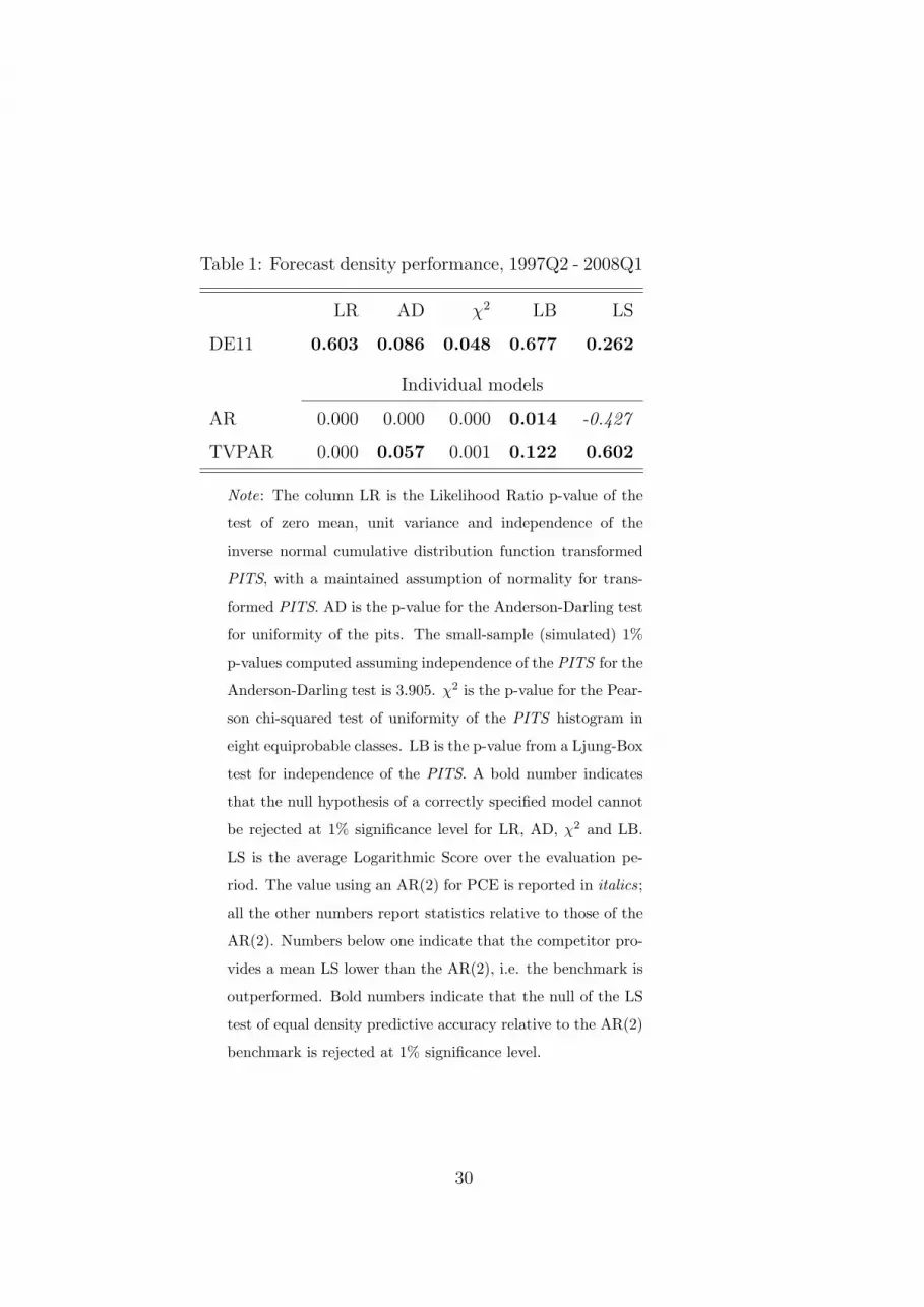
Table 1: Forecast density performance, 1997Q2 - 2008Q1
LR AD χ2 LB LS
DE11 0.603 0.086 0.048 0.677 0.262
Individual models
AR 0.000 0.000 0.000 0.014 -0.427
TVPAR 0.000 0.057 0.001 0.122 0.602
Note: The column LR is the Likelihood Ratio p-value of the
test of zero mean, unit variance and independence of the
inverse normal cumulative distribution function transformed
PITS, with a maintained assumption of normality for trans-
formed PITS. AD is the p-value for the Anderson-Darling test
for uniformity of the pits. The small-sample (simulated) 1%
p-values computed assuming independence of the PITS for the
Anderson-Darling test is 3.905. χ2 is the p-value for the Pear-
son chi-squared test of uniformity of the PITS histogram in
eight equiprobable classes. LB is the p-value from a Ljung-Box
test for independence of the PITS. A bold number indicates
that the null hypothesis of a correctly specified model cannot
be rejected at 1% significance level for LR, AD, χ2 and LB.
LS is the average Logarithmic Score over the evaluation pe-
riod. The value using an AR(2) for PCE is reported in italics;
all the other numbers report statistics relative to those of the
AR(2). Numbers below one indicate that the competitor pro-
vides a mean LS lower than the AR(2), i.e. the benchmark is
outperformed. Bold numbers indicate that the null of the LS
test of equal density predictive accuracy relative to the AR(2)
benchmark is rejected at 1% significance level.
30


