Forecasting Crude Oil Price Movements with Oil-Sensitive

Munich Personal RePEc Archive

Forecasting Crude Oil Price Movements

with Oil-Sensitive Stocks

Chen, Shiu-Sheng

Department of Economics, National Taiwan University

22 August 2013

Online at https://mpra.ub.uni-muenchen.de/49240/

MPRA Paper No. 49240, posted 22 Aug 2013 09:11 UTC

Forecasting Crude Oil Price Movements with

Oil-Sensitive Stocks

Shiu-Sheng Chen∗

August 22, 2013

Abstract

This paper uses monthly data from 1984:M10 to 2012:M8 to show that oil-sensitive

stock price indices, particularly those in the energy sector, have strong power in pre-

dicting nominal and real crude oil prices at short horizons (one-month-ahead predic-

tions), using both in- and out-of-sample tests. In particular, the forecasts based on

oil-sensitive stock price indices are able to outperform significantly the no-change

forecasts. For example, using the NYSE Arca (AMEX) oil index as a predictor, the

one-month-ahead forecasts for nominal crude oil prices reduce the mean squared pre-

diction error by between 22% (for the West Texas Intermediate oil price) and 28%

(for the Dubai oil price). Moreover, we find that the directional forecast based the

AMEX oil index is significantly better than a 50:50 coin toss. The novelty of this

analysis is that it proposes a new and valuable predictor that both reflects timely mar-

ket information and is readily available for forecasting the spot oil price.

Keywords: oil-sensitive stock prices; oil prices; out-of-sample prediction

JEL classification: G17; Q43; Q47; C53

∗Department of Economics, National Taiwan University. I would like to thank two anonymous referees

for comments and suggestions on an earlier version of this paper. Any remaining errors are my own. The

financial assistance of grants from the National Science Council is gratefully acknowledged. Phone number:

(886) 2-2351-9641 ext 481. Address: No. 21, Hsu-Chow Road, Taipei, Taiwan. email: [email protected].

tw

1

1 Introduction

This paper uses monthly data from 1984:M10 to 2012:M8 to investigate the predictive

content of oil-sensitive stock price indices for both nominal and real spot crude oil prices

in both in- and out-of-sample tests. As stock prices are not subject to revision, the proposed

variable, which reflects timely market information and is readily available, can potentially

be a valuable predictor, and thereby help to improve the accuracy of forecasts of the price

of crude oil.

Given that crude oil price is one of the key variables in forecasting macroeconomic

aggregates, including real GDP and inflation (see the discussion in Kilian and Vigfusson

(2011a,b, 2013) and Kilian and Lewis (2011)), the forecasting of crude oil prices has

become the focus of many economists and decision makers (see Alquist et al. (2012)).

The recent literature has already explored the forecasting ability of a number of predictors

for the price of oil, including the oil futures price, oil inventories, the price of crack spread

futures, the price of industrial raw materials (other than crude oil), the dollar exchange rate

of major broad-based commodity exporters, U.S. and global macroeconomic aggregates,

and expert survey forecasts (see Alquist and Kilian (2010), Ye et al. (2005, 2006), Murat

and Tokat (2009), Reeve and Vigfusson (2011), Chen et al. (2010), Baumeister and Kilian

(2012a,b, 2013), Alquist et al. (2012), and the references therein).

The novelty of this paper is to propose a new leading indicator, namely, oil-sensitive

stock price indices, to forecast the price of crude oil instead. This predictor is motivated by

the close link between the stock and oil markets already documented in the existing litera-

ture. Research into the oil price–stock price nexus has been increasing in recent years.1 For

1Early studies analyzing the relationship between oil prices and stock market prices include Kling (1985),

Jones and Kaul (1996), Sadorsky (1999), and El-Sharif et al. (2005).

2

example, see Driesprong et al. (2008), Nandha and Faff (2008), and Park and Ratti (2008).

However, the relationship between oil prices and stock returns is unstable when one does

not control for the composition of oil demand and supply shocks, as emphasized in recent

work by Kilian and Park (2009). They show that the response of aggregate U.S. real stock

returns may differ depending on whether the increase in the price of crude oil is driven by

demand or supply shocks in the crude oil market. In other work, Apergis and Miller (2008)

modify Kilian and Park (2009)’s methodology and investigate data from Australia and G7

countries. They find evidence that different oil market structural shocks play a significant

role in explaining adjustments in stock returns, although the magnitude of such effects

proves to be small. Elsewhere, Narayan and Sharma (2011) find evidence that lagged oil

prices are able to forecast stock returns using returns for 560 U.S. companies listed on

the New York Stock Exchange (NYSE), while Elyasiani et al. (2011) show that oil price

fluctuations constitute systematic asset price risk at the industry level. Lastly, Scholtens

and Yurtsever (2012) investigate the dynamic link between oil prices and stock returns at

the industry level in the Eurozone and conclude that the oil–stock price relationship differs

substantially across industries.

Most studies focus on predicting stock returns using oil prices, with only a few at-

tempting to examine the predictive content of stock returns on the price of crude oil. Ham-

moudeh and Aleisa (2004) present evidence that the Saudi stock index can predict New

York Mercantile Exchange (NYMEX) oil futures prices, while the empirical findings in

Zhang and Wei (2011) suggest that stock market risk in some developed countries (the

U.S., the U.K., and Japan) is able to forecast international crude oil returns constructed

using the West Texas Intermediate (WTI) futures price.

However, to the best of our knowledge, no existing study examines the forecasting

3

content of stock price indices on predicting spot oil prices via in- and out-of-sample tests.

There are several reasons for considering stock prices as predictors of spot crude oil prices.

First, as global stock markets have become more integrated, stock prices should be a re-

liable leading indicator of boom and bust in the economy, respectively resulting in the

increasing and decreasing demand for oil. We thus expect stock prices to predict oil prices

well. Furthermore, Kilian and Vega (2011) show that unlike stock prices, the price of WTI

crude oil does not respond significantly to macroeconomic news in the U.S. within either

the day or the month. Hence, in response to the same macroeconomic news, we expect a

lead–lag relationship between stock prices and oil prices. In particular, we consider oil-

sensitive stock price indices, which may be more informative in tracing future changes

in crude oil prices. Finally, stock prices appear superior as a leading indicator because

timely stock price data are readily available for forecasting purposes. As stock prices are

not subject to revision, the proposed predictor can be used in real-time data forecasts and

even extended to consider price data at higher frequencies. In this paper, we investigate oil

price predictability in terms of both the nominal and real dollar prices of oil. We focus on

forecasting nominal oil prices with nominal returns and on forecasting real oil prices with

real returns. Just as nominal oil price forecasts are of great interest to decision makers,

such as market traders and other economic agents, policy makers, such as central bankers,

may also be concerned about forecasting the real price of oil.

In this paper, the in-sample tests are based on the t-test statistic from a one-month-

ahead predictive regression model, while the out-of-sample prediction performance is

measured using both the mean squared prediction error (MSPE) of the forecasts and their

directional accuracy. We show that regardless of whether the forecasts are for the nominal

or real dollar price of oil, energy sector stock price indices, including those for the NYSE

4

Arca (AMEX) Oil Index and the Morgan Stanley Capital International (MSCI) world en-

ergy sector indices (Energy, Energy Equipment & Services, and Oil & Gas) predict spot

oil prices well and generally outperform the no-change forecast in pseudo out-of-sample

forecast exercises. For example, the reduction in MSPE is shown to be between 22% and

28% for one-month-ahead prediction based on the AMEX oil index. Moreover, we find

that the directional forecast is significantly better than tossing a coin. However, we also

find that the transportation sector fails to provide informative content for the forecasting

of crude oil prices. In general, the results are robust with respect to a variety of crude oil

prices, including the WTI, the U.K. Brent, the Dubai, and the World Average. The findings

of this paper are then of particular interest to market investors and policy makers, given

that oil futures prices often fail to provide accurate predictions, as shown in Alquist et al.

(2012).

The structure of the paper is as follows. Section 2 presents the empirical framework.

Section 3 describes the data and the key empirical results. Section 4 provides some robust-

ness checks. Finally, we offer a conclusion in Section 5.

2 Econometric Framework

2.1 In-Sample Predictive Regression Models

In this paper, we intend to use monthly data to investigate nominal (real) crude oil price

predictability based on nominal (real) oil-sensitive stock prices. We consider the following

one-month-ahead predictive regression model for in-sample tests:

yt+1 = α + βxt + ut+1. (1)

When investigating nominal oil price predictability, let yt = (opt − opt−1)/opt−1 be the

percentage change in nominal oil prices, where opt is the spot crude oil price. Moreover,

5

let xt = (spt − spt−1)/spt−1 be the nominal stock return, where spt is the stock price index.

When the focus is on forecasting real prices of oil, we construct yt = (ropt−ropt−1)/ropt−1

and xt = (rspt − rspt−1)/rspt−1, where ropt = opt/cpit and rsp = spt/cpit are real oil and

real stock prices, respectively. The term cpit represents the U.S. consumer price index.

We conduct an in-sample test as a test of the null hypothesis of no predictive power

for future oil price movements: β = 0 against the alternative hypothesis, β , 0. Thus, we

evaluate the predictability of the stock return, xt using a t-statistic corresponding to β with

Newey–West heteroscedasticity and autocorrelation consistent (HAC) standard errors.

2.2 Out-of-Sample Forecasts

We now move focus to out-of-sample tests to evaluate oil price predictability. Instead of

forecasting the percentage change in the oil price, the out-of-sample oil price predictability

is now evaluated in terms of the (nominal or real) dollar price of oil as in Baumeister

and Kilian (2012a,b, 2013) because the level of the oil price is the one that matters most

in decision making.2 The total sample of T observations is divided into in- and out-of-

sample portions. There are R in-sample observations, t = 1, ....,R, and P out-of-sample

observations, t = R+1, ....,R+P. Obviously, R+P = T . Consider the following predictive

regression model for the percentage change in the nominal oil price:

yt+h = α + βxt + ut+h, t = R,R + 1, . . . , T − h, (2)

where:

yt+h =opt+h − opt

opt, xt =

spt − spt−1

spt−1

.

2The results are quantitatively similar when considering forecasts of the percentage change in the oil

price.

6

The h-step-ahead pseudo out-of-sample forecast of the crude oil return is obtained by:

yt+h =opt+h − opt

opt= αt + βtxt,

where αt and βt are estimated by a recursive scheme. Hence, the forecast of the nominal

spot price of crude oil is then constructed by:

opt+h = (1 + αt + βtxt) × opt. (3)

To forecast the real spot price of crude oil, we reconstruct yt+h and xt accordingly as:

yt+h =ropt+h − ropt

ropt, xt =

rspt − rspt−1

rspt−1

.

The forecast horizon h is 1, 3, 6, 9, and 12 months.

The benchmark for forecasts based on the price of oil-sensitive stock is provided by

the no-change forecast (the driftless random walk model), which suggests that the best

forecast of the spot oil price is simply the current spot price; that is:

opt+h = opt, (4)

and

ropt+h = ropt, (5)

for the nominal and real prices of oil, respectively.

To evaluate the out-of-sample forecasting accuracy, we use the MSPE as a measure

of prediction performance. Letting MNC and MS P denote the no-change forecast and

the predictive regression model based on the oil-sensitive stock price, respectively, we

compute the MSPE ratio as:

MSPE(MS P)

MSPE(MNC).

Clearly, if the oil-sensitive stock price has a lower MSPE than the no-change forecast, the

MSPE ratio will be less than one. To assess whether the difference between MSPE(MS P)

7

and MSPE(MNC) is statistically significant, we formally test the null hypothesis of equal

forecasting accuracy that MSPE(MS P) = MSPE(MNC) against the alternative hypothesis

that the candidate model is more accurate than the no-change forecast: MSPE(MS P) <

MSPE(MNC), using the bootstrap Diebold and Mariano (1995) test statistic and the boot-

strap Clark and West (2007) MSPE-adjusted test statistic.

In addition to examining the MSPE ratio, we also consider the directional accuracy

of the forecasts, as measured by the success (hit) ratio indicating the relative frequency

with which the predictive regression model based on the oil-sensitive stock price is able

to predict correctly the sign of the change in the oil price. The success ratio is formally

evaluated using the test proposed by Pesaran and Timmermann (2009).

3 Data and Empirical Results

3.1 Data

We employ monthly data from 1984:M10 to 2012:M8 given considerations of data avail-

ability. The oil-sensitive stock price index with the longest sample period available is the

AMEX oil index, which is a price-weighted index of the leading companies involved in

the exploration, production, and development of petroleum. The components of the index

are listed in Table 1.3

Moreover, to show the usefulness of the oil-sensitive stock prices for forecasting crude

oil prices, we use the S&P 500 price index for the purpose of comparison. Finally, as a

sensitivity analysis, we have also considered the oil-sensitive stock prices obtained from

the MSCI World Sector Indices, which are constructed using the Global Industry Classifi-

3We employ a series of stock returns without any adjustment for dividends and stock splits because the

adjusted data for AMEX oil index are not available. We compute the return as the exact percentage change

in the stock price.

8

cation Standard (GICS) with a shorter sample period starting from 1995:M1.4 The MSCI

World Index, covering over 6,000 securities in 24 developed markets and spanning large,

medium, small and micro-cap securities, is generally considered representative of global

market conditions. The oil-sensitive sectors that we include are: (1) Energy sector with

subitems (1.1) Energy Equipment & Services and (1.2) Oil & Gas, as well as (2) Trans-

portation sector with subitems (2.1) Air Freight & Logistics, (2.2) Airlines, (2.3) Marine,

and (2.4) Road & Rail. The Energy Sector comprises companies whose businesses are

dominated by energy activities:

1. Manufacturers of oil rigs and drilling equipment, and providers of drilling services.

2. Manufacturers of equipment for and providers of services to the oil and gas indus-

try not classified elsewhere, including companies providing seismic data collection

services.

3. Integrated oil companies engaged in the exploration, production, refinement, and

distribution of oil and gas products.

4. Companies engaged in the exploration and production of oil and gas not classified

elsewhere.

5. Companies engaged in the refining, marketing and/or transportation of oil and gas

products.

The Transportation Sector comprises companies whose businesses are dominated by trans-

portation activities:

1. Companies providing airfreight transportation, courier and logistics services, includ-

ing package and mail delivery and customs agents.

2. Companies providing primarily passenger air transportation.

3. Companies providing goods or passenger maritime transportation.

4The MSCI World Sector Indices are not used for the baseline results because the sample span is smaller.

9

4. Companies providing primarily goods and passenger rail transportation.

5. Companies providing primarily goods and passenger land transportation, including

vehicle rental and taxi companies.

We obtain the AMEX oil index, and the S&P 500 price index from Yahoo Finance.

The MSCI World Sector Indices are from Datastream. The crude oil price data that we

consider are for the prices of WTI, U.K. Brent, United Arab Emirates Dubai, and World

Average oil, all of which are available from the International Financial Statistics (IFS)

published by the International Monetary Fund. The world average crude price is an equal-

weighted average of the U.K. Brent (light), Dubai (medium), and WTI prices. The U.S.

consumer price index is from the Federal Reserve Economic Data (FRED). Table 2 details

the variable names, data codes, and sample periods. The three measures of crude oil prices

are shown in Figure 1. Figure 2 depicts the AMEX oil index and the S&P 500 price index,

and 3 plots all of the MSCI world sector indices.

3.2 In-Sample Predictive Regression Results

The estimates of the predictive regression model in equation (1), including coefficient esti-

mates, t-statistics, and p-values, are reported in Tables 3 and 4 for nominal and real prices

of crude oil, respectively. The Newey–West HAC standard errors employ the Bartlett ker-

nel. The truncation parameter m is determined by m = 0.75T 1/3, rounded to the nearest

integer.

According to the baseline results, the estimates of β for the AMEX oil index are all pos-

itive and statistically significant, which suggests that higher values of oil-sensitive stock

returns predict the higher growth rate of crude oil prices. Different forecasting objec-

tives (nominal vs. real) and different measures of crude oil prices provide similar results.

The positive dynamic correlation is consistent with our expectations. That is, as stock

10

prices are strongly forward looking, expected positive shocks (for instance, good news

about future global demand or macroeconomic conditions) that induce higher oil demand

will increase current oil-sensitive stock returns and thus result in a higher oil price. That

is, the empirical results presented here are dominated by the flow demand shock (shock

to the amount of oil being consumed) discussed in Kilian and Park (2009) and Kilian

and Murphy (2012a,b). The evidence of significant predictive power for future oil price

movements is consistent with the findings of Kilian and Vega (2011) in that there is no

systematic feedback from news about a wide range of U.S. macroeconomic aggregates to

the price of oil between one day and one month, whereas stock prices incorporate infor-

mation about future macroeconomic conditions instantaneously. Hence, in response to the

same macroeconomic news, we should expect that the stock price leads the crude oil price

and that such a lead–lag relationship may be more prominent when the stock considered

is oil sensitive. As a comparison, we observe that the S&P 500, a non-oil-sensitive stock

price index, does not have any significant in-sample predictive power.

Moreover, investigating each MSCI stock return in turn shows that the MSCI world

energy sector indices (Energy, Energy Equipment & Services, and Oil & Gas) produce

consistently strong results across the crude oil prices considered, while one of the trans-

portation sector indices (Marine) provides somewhat weaker evidence. In contrast, three

MSCI world transportation sector indices (Transportation, Air Freight & Logistics and

Road & Rail) do not have significant predictive power. It is then natural to ask: why does

the Energy sector provide strong predictive power while the Transportation sector does

not, and under the Transportation sector, why does the Marine sector provide some pre-

dictive power while the Air Freight & Logistics and Road & Rail sectors do not? Possible

explanations for the sectoral differences may be as follows. First, the companies com-

11

prising the Energy, Energy Equipment & Services, and the Oil & Gas sectors represent the

supply side of the oil market, whereas the companies comprising Transportation industries

mostly represent the demand side of the market. While on the one hand, future booms in

global oil demand, which push up oil prices, may stimulate the stock prices of both the

energy and transportation industries (positive impacts), on the other hand, we also expect

the higher oil price to erode profits in transportation industries and thereby to lower their

stock prices (negative impacts). Hence, the positive and negative effects may cancel each

other out in the Transportation sector, and we may find that the Transportation sector as

a whole has insignificant forecasting power. Moreover, within the Transportation sector,

the reason that the Marine sector can better forecast spot oil prices may be because the

transports of crude oil and refined product heavily rely on marine transportation, which

suggests that the positive impact from increased oil demand may dominate the results for

the Marine transportation sector.

Two other remarks are worth noting. First, we augment the simple predictive regres-

sion model in equation (1) with autoregressive terms to obtain an autoregressive distributed

lag (ARDL) predictive regression model:

yt+1 = α +

p∑

j=0

β jxt−p +

p∑

j=0

γ jyt−p + ut+1,

as a robustness check of the empirical results. We select the number of lags p using

the Akaike Information Criterion. The in-sample predictive ability is assessed by test-

ing H0: β0 = 0, and the findings are similar to those in Tables 3 and 4. Second, it is

of interest to confirm whether the relationship between oil-sensitive stock prices and spot

oil prices has changed over the sample periods that we consider in this analysis. The

Andrews–Quandt tests developed by Andrews (1993) suggest no evidence of the presence

of structural breaks at an unknown date within the sample period considered. Using the

12

relationship between nominal WTI oil price and the nominal AMEX oil index as an exam-

ple, the Andrews–Quandt test statistic is 5.12 with a p-value of 0.54, suggesting that we

cannot reject the null hypothesis of no structural change .5

In sum, we find that oil-sensitive stock returns, particularly the U.S. AMEX Oil Index

and the MSCI world energy sector provide useful information for forecasting the percent-

age changes in crude oil via in-sample predictive regressions. The empirical evidence on

the predictability of the oil-sensitive stock is robust with respect to different forecasting

objectives (nominal vs. real), different measures of crude oil prices, and different model

specification. Moreover, the predictive relationship between the oil-sensitive stock return

and the percentage change in the crude oil price is stable over time.

3.3 Out-of-Sample Forecasting Performance

We now turn to the evidence obtained from the out-of-sample forecasting tests. As well

documented in the literature, in-sample predictability does not necessarily translate into

out-of-sample forecasting ability (see Inoue and Kilian (2004)). Accordingly, we would

like to appreciate whether the in-sample oil price predictability found above holds in an

out-of-sample forecasting exercise.

Recall that R represents the sample size for in-sample estimation (model specifica-

tion/estimation/training period), and P is the number of out-of-sample observations (model

comparison/evaluation/validation period). The out-of-sample results are obtained by set-

ting the out-of-sample period to 1991:M1–2012:M8, so that the starting date for the fore-

cast evaluation matches what Alquist et al. (2012) and Baumeister and Kilian (2012b)

use. Initially we use 75 observations to estimate the predictive regression model. The

5Detailed results supporting both of the above remarks are available upon request.

13

out-of-sample forecast results are obtained based on the recursive estimation scheme.6

Table 5 shows that at short horizons (one and three months), the forecasts for nominal

crude oil price levels based on the AMEX oil index produce lower MSPEs than the no-

change forecast. For example, the one-month-ahead forecasts for nominal crude oil prices

reduce the MSPEs by between 22% (for the WTI price of oil) and 28% (for the Dubai

price of oil). These results are statistically significant at the 5% level. For the three-month

forecast horizon, the reductions in MSPE are somewhat smaller (between 5% and 8%),

but still statistically significant. However, for the longer forecast horizons of 6, 9, and 12

months, the oil-sensitive stock price fails to beat the benchmark no-change forecast.

Regarding the accuracy of the directional forecasts, the success ratios are all superior to

tossing a coin (50%) at all horizons considered. For example, the probability of correctly

predicting the direction of change at horizons of 1, 3, 6, 9, and 12 months is 63%, 57%,

54%, 53%, and 53%, respectively, for the WTI price of oil, though statistically significant

directional accuracy is only obtained at the one-month horizon. Different measures of the

crude oil price provide similar evidence. According to the bottom panel in Table 5, the

out-of-sample test results for real oil prices generally exhibit patterns similar to the results

from forecasting the nominal price of oil. That is, we may conclude that the oil-sensitive

stock price contains out-of-sample forecasting power for nominal as well as real prices of

crude oil at short horizons (one month).

The empirical results from the MSCI indices with shorter sample span (limited to

1995:M1–2012:M8) are reported in Tables 6 and 7. The forecast evaluation period is

2002M1–2012M8 so that initially we have 84 observations to estimate the model parame-

ters. Tables 6 and 7 show that for the one-month forecast horizon (h = 1), the MSCI world

6Using a rolling estimation scheme does not substantially alter the empirical results.

14

energy sector indices and the MSCI marine index outperform the no-change forecast with

statistical significance in terms of the MSPE criterion and the forecasting performance of

the directional change in the price of oil. These results are robust, regardless of whether

the focus is on the nominal or real price of oil. However, the evidence supporting a fore-

cast horizon longer than one month exhibits patterns similar to those obtained in Table 5

and indicates no predictive power as based on the MSCI indices.

In sum, we have found strong evidence that the U.S. AMEX Oil Index and the MSCI

world energy sector stock price index help to forecast crude oil prices (nominal and real)

out-of-sample at short horizons (one month).

4 Robustness Checks

To check the robustness of our empirical results, we consider the following modifications

of the forecasting exercise. First, we consider different forecasting validation periods; i.e.,

different P/R ratios. Second, we include additional data in the form of the MSCI Energy

Sector Indices for All Country World, Europe, and Emerging Markets. Finally, we include

the oil futures–spot spread to see whether stock returns contain additional information

beyond that in futures prices. In this section, we only report the results for the one-month-

ahead forecasts (h = 1) as the model does not have significant predictive power for longer

forecasting horizons, as shown previously.

4.1 Alternative Forecasting Validation Periods

In the baseline out-of-sample forecasting exercise, the forecast evaluation period is 1991:M1–

2012:M8, which implies P/R ≈ 3.55, where P is the number of out-of-sample observations

and R is the sample size for the in-sample estimation. We now consider P/R = 0.5, 1.0,

15

1.5, 2.0, and 3.0, and thus the corresponding starting dates for the evaluation are 2003:M6,

1998:M11, 1996:M1, 1994:M3, and 1991:M11, respectively. Table 8 reports the results

and shows that our earlier conclusions are robust with respect to different P/R ratios.

4.2 Alternative Stock Price Indices

We examined oil-sensitive stock returns using the MSCI World Sector Index, which only

includes developed markets. To check for robustness, we further consider the following

indices: (1) the MSCI All Country World Index (ACWI), which incorporates both de-

veloped and emerging countries, (2) the MSCI Europe Index, which measures the equity

market performance of developed markets in Europe, and (3) the MSCI Emerging Markets

(EM) Index, which covers over 2,700 securities in 21 markets currently classified as EM

countries.

For the in-sample predictive regressions, we report the t-statistics for testing β = 0 in

equation (1). For the out-of-sample forecasting tests, we report the MSPE ratio and the

success ratio. The results reported in Tables 9 and 10 show that for both the in-sample pre-

dictive regressions and the out-of-sample forecast comparisons, our previous conclusions

remain strong and significant.

4.3 Adding Information from Oil Futures Prices

As the prices of oil futures contracts are widely used in the existing literature to forecast

future spot oil prices, we question whether the strong predictive power of oil-sensitive

stock returns suggested in this analysis remain after accounting for the forecasting content

in futures prices. That is, we would like to know what, if any, additional information

oil-sensitive stock prices contain beyond the futures prices of crude oil. We consider the

16

following regression model:

yt+1 = α + βxt + θξt + ut+1, (6)

where ξt = ( ft,t+1 − opt)/opt represents the oil futures–spot spread, and ft,t+1 denotes the

current price of an oil futures contract that matures in one month (the one-month-ahead

futures price). We use the NYMEX one-month-ahead crude oil futures price data for

the WTI (Light-Sweet, Cushing, Oklahoma) available from the U.S. Energy Information

Administration.

For forecasting the one-month-ahead nominal WTI price of oil using the AMEX oil

index as a predictor from 1984:M10 to 2012:M8, we find that the t-statistics is 3.89 for the

in-sample test. The MSPE ratio is 0.78, which suggests a 22% reduction in MSPE. The

success ratio equals 0.62 and shows that the directional forecast is better than a coin toss.

Both the MSPE and success ratios are statistically significant at the 5% level. Clearly, in

both in- and out-of-sample tests, the AMEX oil index has strong predictive power for the

spot oil price, even after conditioning on the price of oil futures contracts.

5 Conclusion

This paper focuses on the dynamic relationship between crude oil prices and oil-sensitive

stock prices. We investigate the predictive content of oil-sensitive stock price indices for

crude oil prices using in- and out-of-sample tests. The baseline findings with monthly

data from 1984:M10 to 2012:M8 show that the AMEX oil index indeed provides useful

information in forecasting crude oil prices via in-sample predictive regressions. Moreover,

using both MSPE and directional forecast accuracy as criteria of forecasting performance,

the AMEX oil index outperforms the no-change forecasts in the pseudo out-of-sample

forecast exercises at horizon one (the one-month-ahead forecast). The MSPE reductions

17

are between 22% to 28% for forecasting nominal oil price, while the reductions are up

to 26% for forecasting real oil prices. Moreover, the one-month-ahead forecasts based on

the AMEX oil index have higher directional accuracy than tossing a coin. Both the MSPE

reductions and the directional accuracy are statistically significant. We have also examined

the MSCI world sector indices with a shorter sample span from 1995:M1 to 2012:M8 as

a sensitive analysis and found that the MSCI world energy sector indices (Energy, Energy

Equipment & Services, and Oil & Gas) have strong in-sample and out-of-sample predictive

power. However, the evidence also shows that the transportation sector stock price does

not forecast oil prices well.

Our results are quite robust with respect to different measures of crude oil prices (WTI,

Brent, Dubai, and World Average), a variety of model validation periods, diverse estima-

tion schemes, and a range of sample periods. Finally, we find that oil-sensitive stock prices

contain substantial additional information beyond that found in oil futures prices.

The novelty of the current paper is that it proposes a new and valuable predictor, which

reflects timely market information and is readily available, for forecasting short-run oil

price movements. As stock prices are not subject to revision, the proposed predictor can

be used in real-time data forecasts and can be extended to incorporate even higher frequen-

cies. The evidence provided in the current paper is thus of particular interest to market

investors and policy makers given that oil futures prices typically fail to provide accurate

predictions.

18

References

Alquist, Ron and Kilian, Lutz (2010), “What do we learn from the price of crude oil

futures?”, Journal of Applied Econometrics, 25(4), 539 – 573.

Alquist, Ron, Kilian, Lutz, and Vigfusson, Robert J. (2012), “Forecasting the price of

oil”, in G. Elliott and A. Timmermann (eds.), forthcoming, Handbook of Economic

Forecasting, volume 2, Amsterdam: North-Holland.

Andrews, Donald W. K. (1993), “Tests for parameter instability and structural change with

unknown change point”, Econometrica, 61(4), 821–856.

Apergis, Nicholas and Miller, Stephen M. (2008), “Do structural oil-market shocks affect

stock prices?”, Energy Economics, 31(4), 569–575.

Baumeister, Christiane and Kilian, Lutz (2012a), “Real-time analysis of oil price risks

using forecast scenarios”, Working Papers 2012-1, Bank of Canada.

(2012b), “Real-time forecasts of the real price of oil”, Journal of Business and

Economic Statistics, 30(2), 326–336.

(2013), “What central bankers need to know about forecasting oil prices”, mimeo,

University of Michigan.

Chen, Yu-Chin, Rogoff, Kenneth S., and Rossi, Barbara (2010), “Can exchange rates fore-

cast commodity prices?”, The Quarterly Journal of Economics, 125(3), 1145–1194.

Clark, Todd E. and West, Kenneth D. (2007), “Approximately normal tests for equal pre-

dictive accuracy in nested models”, Journal of Econometrics, 138(1), 291–311.

19

Diebold, F.X. and Mariano, R.S. (1995), “Comparing predictive accuracy”, Journal of

Business and Economic Statistics, 13, 253–263.

Driesprong, Gerben, Jacobsen, Ben, and Maat, Benjamin (2008), “Striking oil: Another

puzzle?”, Journal of Financial Economics, 89(2), 307 – 327.

El-Sharif, Idris, Brown, Dick, Burton, Bruce, Nixon, Bill, and Russell, Alex (2005), “Ev-

idence on the nature and extent of the relationship between oil prices and equity values

in the UK”, Energy Economics, 27(6), 819 – 830.

Elyasiani, Elyas, Mansur, Iqbal, and Odusami, Babatunde (2011), “Oil price shocks and

industry stock returns”, Energy Economics, 33(5), 966 – 974.

Hammoudeh, Shawkat and Aleisa, Eisa (2004), “Dynamic relationships among GCC stock

markets and NYMEX oil futures”, Contemporary Economic Policy, 22(2), 250–269.

Inoue, Atsushi and Kilian, Lutz (2004), “In-sample or out-of-sample tests of predictability:

Which one should we use?”, Econometric Reviews, 23(4), 371–402.

Jones, Charles M and Kaul, Gautam (1996), “Oil and the stock markets”, Journal of Fi-

nance, 51(2), 463–91.

Kilian, Lutz and Lewis, Logan T. (2011), “Does the Fed respond to oil price shocks?”,

Economic Journal, 121(555), 1047–1072.

Kilian, Lutz and Murphy, Dan (2012a), “The role of inventories and speculative trading in

the global market for crude oil”, forthcoming, Journal of Applied Econometrics.

Kilian, Lutz and Murphy, Daniel P. (2012b), “Why agnostic sign restrictions are not

enough: Understanding the dynamics of oil market VAR models”, Journal of the Euro-

pean Economic Association, 10(5), 1166–1188.

20

Kilian, Lutz and Park, Cheolbeom (2009), “The impact of oil price shocks on the U.S.

stock market”, International Economic Review, 50(4), 1267–1287.

Kilian, Lutz and Vega, Clara (2011), “Do energy prices respond to U.S. macroeconomic

news? a test of the hypothesis of predetermined energy prices”, The Review of Eco-

nomics and Statistics, 93(2), 660–671.

Kilian, Lutz and Vigfusson, Robert J. (2011a), “Are the responses of the U.S. economy

asymmetric in energy price increases and decreases?”, Quantitative Economics, 2(3),

419–453.

(2011b), “Nonlinearities in the oil price–output relationship”, Macroeconomic Dy-

namics, 15(S3), 337–363.

(2013), “Do oil prices help forecast U.S. real GDP? the role of nonlinearities and

asymmetries”, Journal of Business & Economic Statistics, 31(1), 78–93.

Kling, John L. (1985), “Oil price shocks and stock market behavior”, The Journal of Port-

folio Management, 12(1), 34–39.

Murat, Atilim and Tokat, Ekin (2009), “Forecasting oil price movements with crack spread

futures”, Energy Economics, 31(1), 85–90.

Nandha, Mohan and Faff, Robert (2008), “Does oil move equity prices? a global view”,

Energy Economics, 30(3), 986 – 997.

Narayan, Paresh Kumar and Sharma, Susan Sunila (2011), “New evidence on oil price and

firm returns”, Journal of Banking and Finance, 35(12), 3253 – 3262.

Park, Jungwook and Ratti, Ronald A. (2008), “Oil price shocks and stock markets in the

U.S. and 13 European countries”, Energy Economics, 30(5), 2587 – 2608.

21

Pesaran, M. Hashem and Timmermann, Allan (2009), “Testing dependence among serially

correlated multicategory variables”, Journal of the American Statistical Association,

104(485), 325–337.

Reeve, Trevor A. and Vigfusson, Robert J. (2011), “Evaluating the forecasting perfor-

mance of commodity futures prices”, International Finance Discussion Papers, Board

of Governors of the Federal Reserve System 1025, URL: http://ideas.repec.org/

p/fip/fedgif/1025.html.

Sadorsky, Perry (1999), “Oil price shocks and stock market activity”, Energy Economics,

21(5), 449 – 469.

Scholtens, Bert and Yurtsever, Cenk (2012), “Oil price shocks and European industries”,

Energy Economics, 34(4), 1187 – 1195.

Ye, Michael, Zyren, John, and Shore, Joanne (2005), “A monthly crude oil spot price fore-

casting model using relative inventories”, International Journal of Forecasting, 21(3),

491 – 501.

(2006), “Forecasting short-run crude oil price using high- and low-inventory vari-

ables”, Energy Policy, 34(17), 2736–2743.

Zhang, Yue-Jun and Wei, Yi-Ming (2011), “The dynamic influence of advanced stock mar-

ket risk on international crude oil returns: an empirical analysis”, Quantitative Finance,

11(7), 967–978.

22

Table 1: AMEX Oil Index Components

Company Name Symbol

Anadarko Petroleum Corporation APC

BP plc BP

ConocoPhillips COP

Chevron Corporation CVX

Hess Corporation HES

Marathon Oil Corporation MRO

Occidental Petroleum Corporation OXY

Petr PBR

Phillips 66 PSX

Total SA TOT

Valero Energy Corporation VLO

Exxon Mobil Corporation XOM

Table 2: Description of Data

Variables Code Source

Baseline (1984M10–2012M8)

WTI 11176AAZZFM17 IFS

Brent 11276AAZZF... IFS

Dubai 46676AAZZF... IFS

World Average 00176AAZZF... IFS

AMEX Oil Index ˆXOI Yahoo Finance

S&P 500 ˆGSPC Yahoo Finance

U.S. Consumer Price Index CPIAUCSL FRED

MSCI World Sector Index (1995M1–2012M8 )

(1) Energy M1DWE1$ Datastream

(1.1) Energy Equipment & Services M3DWES$ Datastream

(1.2) Oil & Gas M3DWOG$ Datastream

(2) Transportation M2DWTR$ Datastream

(2.1) Air Freight & Logistics M3DWAF$ Datastream

(2.2) Airlines M3DWAL$ Datastream

(2.3) Marine M3DWMA$ Datastream

(2.4) Road & Rail M3DWRR$ Datastream

23

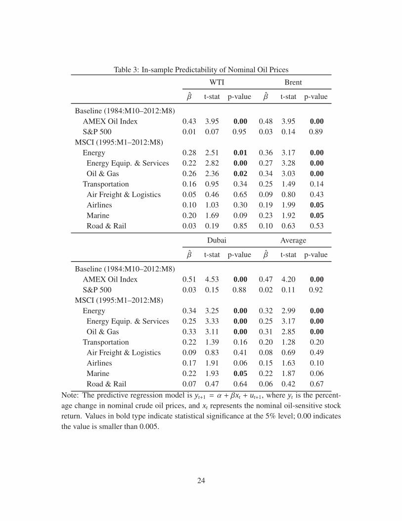
Table 3: In-sample Predictability of Nominal Oil Prices

WTI Brent

β t-stat p-value β t-stat p-value

Baseline (1984:M10–2012:M8)

AMEX Oil Index 0.43 3.95 0.00 0.48 3.95 0.00S&P 500 0.01 0.07 0.95 0.03 0.14 0.89

MSCI (1995:M1–2012:M8)

Energy 0.28 2.51 0.01 0.36 3.17 0.00Energy Equip. & Services 0.22 2.82 0.00 0.27 3.28 0.00Oil & Gas 0.26 2.36 0.02 0.34 3.03 0.00

Transportation 0.16 0.95 0.34 0.25 1.49 0.14

Air Freight & Logistics 0.05 0.46 0.65 0.09 0.80 0.43

Airlines 0.10 1.03 0.30 0.19 1.99 0.05Marine 0.20 1.69 0.09 0.23 1.92 0.05Road & Rail 0.03 0.19 0.85 0.10 0.63 0.53

Dubai Average


Baseline (1984:M10–2012:M8)

AMEX Oil Index 0.51 4.53 0.00 0.47 4.20 0.00S&P 500 0.03 0.15 0.88 0.02 0.11 0.92

MSCI (1995:M1–2012:M8)


Transportation 0.22 1.39 0.16 0.20 1.28 0.20


Airlines 0.17 1.91 0.06 0.15 1.63 0.10

Marine 0.22 1.93 0.05 0.22 1.87 0.06

Road & Rail 0.07 0.47 0.64 0.06 0.42 0.67

Note: The predictive regression model is yt+1 = α + βxt + ut+1, where yt is the percent-

age change in nominal crude oil prices, and xt represents the nominal oil-sensitive stock

return. Values in bold type indicate statistical significance at the 5% level; 0.00 indicates

the value is smaller than 0.005.

24

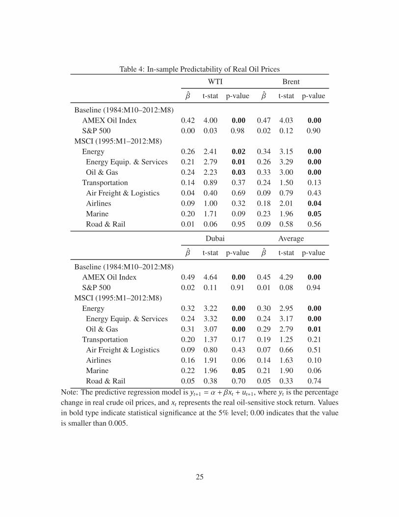
Table 4: In-sample Predictability of Real Oil Prices

WTI Brent


Baseline (1984:M10–2012:M8)

AMEX Oil Index 0.42 4.00 0.00 0.47 4.03 0.00S&P 500 0.00 0.03 0.98 0.02 0.12 0.90

MSCI (1995:M1–2012:M8)


Transportation 0.14 0.89 0.37 0.24 1.50 0.13


Airlines 0.09 1.00 0.32 0.18 2.01 0.04Marine 0.20 1.71 0.09 0.23 1.96 0.05Road & Rail 0.01 0.06 0.95 0.09 0.58 0.56

Dubai Average


Baseline (1984:M10–2012:M8)

AMEX Oil Index 0.49 4.64 0.00 0.45 4.29 0.00S&P 500 0.02 0.11 0.91 0.01 0.08 0.94

MSCI (1995:M1–2012:M8)


Transportation 0.20 1.37 0.17 0.19 1.25 0.21


Airlines 0.16 1.91 0.06 0.14 1.63 0.10

Marine 0.22 1.96 0.05 0.21 1.90 0.06

Road & Rail 0.05 0.38 0.70 0.05 0.33 0.74

Note: The predictive regression model is yt+1 = α + βxt + ut+1, where yt is the percentage

change in real crude oil prices, and xt represents the real oil-sensitive stock return. Values

in bold type indicate statistical significance at the 5% level; 0.00 indicates that the value

is smaller than 0.005.

25

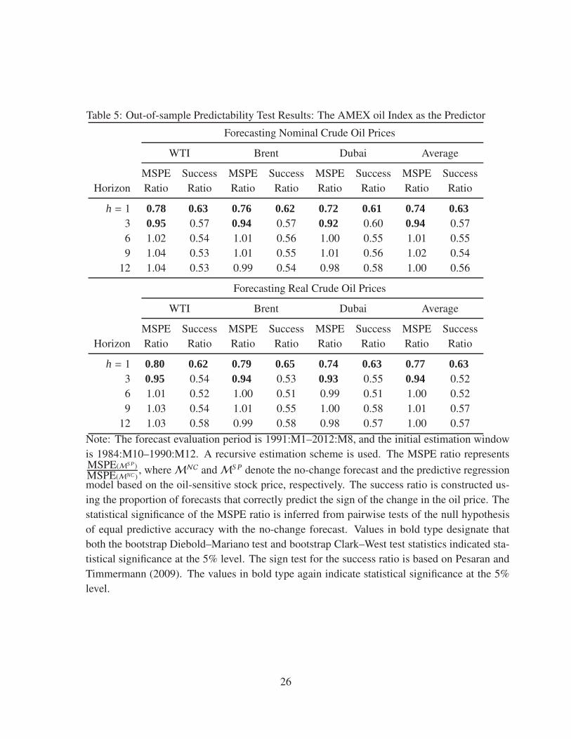
Table 5: Out-of-sample Predictability Test Results: The AMEX oil Index as the Predictor

Forecasting Nominal Crude Oil Prices

WTI Brent Dubai Average

MSPE Success MSPE Success MSPE Success MSPE Success

Horizon Ratio Ratio Ratio Ratio Ratio Ratio Ratio Ratio

h = 1 0.78 0.63 0.76 0.62 0.72 0.61 0.74 0.633 0.95 0.57 0.94 0.57 0.92 0.60 0.94 0.57

6 1.02 0.54 1.01 0.56 1.00 0.55 1.01 0.55

9 1.04 0.53 1.01 0.55 1.01 0.56 1.02 0.54

12 1.04 0.53 0.99 0.54 0.98 0.58 1.00 0.56

Forecasting Real Crude Oil Prices




h = 1 0.80 0.62 0.79 0.65 0.74 0.63 0.77 0.633 0.95 0.54 0.94 0.53 0.93 0.55 0.94 0.52

6 1.01 0.52 1.00 0.51 0.99 0.51 1.00 0.52

9 1.03 0.54 1.01 0.55 1.00 0.58 1.01 0.57

12 1.03 0.58 0.99 0.58 0.98 0.57 1.00 0.57

Note: The forecast evaluation period is 1991:M1–2012:M8, and the initial estimation window

is 1984:M10–1990:M12. A recursive estimation scheme is used. The MSPE ratio representsMSPE(MS P)

MSPE(MNC ), whereMNC andMS P denote the no-change forecast and the predictive regression

model based on the oil-sensitive stock price, respectively. The success ratio is constructed us-

ing the proportion of forecasts that correctly predict the sign of the change in the oil price. The

statistical significance of the MSPE ratio is inferred from pairwise tests of the null hypothesis

of equal predictive accuracy with the no-change forecast. Values in bold type designate that

both the bootstrap Diebold–Mariano test and bootstrap Clark–West test statistics indicated sta-

tistical significance at the 5% level. The sign test for the success ratio is based on Pesaran and

Timmermann (2009). The values in bold type again indicate statistical significance at the 5%

level.

26

Table 6: Out-of-sample Predictability Test Results: The MSCI Sector Indices as the Predictors

Forecasting Nominal Crude Oil Prices (Forecasting Horizon h = 1)




MSCI (1995:M1–2012:M8)

Energy 0.90 0.66 0.86 0.68 0.84 0.69 0.86 0.66Energy Equip. & Services 0.89 0.64 0.85 0.62 0.83 0.66 0.85 0.65Oil & Gas 0.91 0.66 0.87 0.66 0.86 0.69 0.88 0.67

Transportation 1.00 0.60 0.97 0.60 0.98 0.63 0.98 0.61

Air Freight & Logistics 1.04 0.63 1.02 0.60 1.02 0.63 1.03 0.61

Airlines 1.02 0.66 1.01 0.59 1.00 0.66 1.01 0.64

Marine 0.96 0.63 0.94 0.60 0.93 0.63 0.94 0.63

Road & Rail 1.04 0.58 1.01 0.59 1.03 0.59 1.03 0.59

Note: The forecast evaluation period is 1991:M1–2012:M8, and the initial estimation window is 1984:M10–

1990:M12. A recursive estimation scheme is used. The MSPE ratio represents MSPE(MS P)

MSPE(MNC), where MNC and

MS P denote the no-change forecast and the predictive regression model based on the oil-sensitive stock price,

respectively. The success ratio is constructed using the proportion of forecasts that correctly predict the sign of

the change in the oil price. The statistical significance of the MSPE ratio is inferred from pairwise tests of the

null hypothesis of equal predictive accuracy with the no-change forecast. Values in bold type designate that both

the bootstrap Diebold–Mariano test and bootstrap Clark–West test statistics indicated statistical significance at

the 5% level. The sign test for the success ratio is based on Pesaran and Timmermann (2009). The values in bold

type again indicate statistical significance at the 5% level.

27

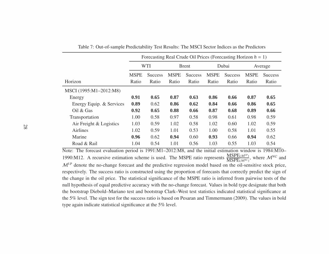
Table 7: Out-of-sample Predictability Test Results: The MSCI Sector Indices as the Predictors

Forecasting Real Crude Oil Prices (Forecasting Horizon h = 1)




MSCI (1995:M1–2012:M8)

Energy 0.91 0.65 0.87 0.63 0.86 0.66 0.87 0.65Energy Equip. & Services 0.89 0.62 0.86 0.62 0.84 0.66 0.86 0.65Oil & Gas 0.92 0.65 0.88 0.66 0.87 0.68 0.89 0.66

Transportation 1.00 0.58 0.97 0.58 0.98 0.61 0.98 0.59

Air Freight & Logistics 1.03 0.59 1.02 0.58 1.02 0.60 1.02 0.59

Airlines 1.02 0.59 1.01 0.53 1.00 0.58 1.01 0.55

Marine 0.96 0.62 0.94 0.60 0.93 0.66 0.94 0.62

Road & Rail 1.04 0.54 1.01 0.56 1.03 0.55 1.03 0.54

Note: The forecast evaluation period is 1991:M1–2012:M8, and the initial estimation window is 1984:M10–

1990:M12. A recursive estimation scheme is used. The MSPE ratio represents MSPE(MS P)

MSPE(MNC), where MNC and

MS P denote the no-change forecast and the predictive regression model based on the oil-sensitive stock price,

respectively. The success ratio is constructed using the proportion of forecasts that correctly predict the sign of

the change in the oil price. The statistical significance of the MSPE ratio is inferred from pairwise tests of the

null hypothesis of equal predictive accuracy with the no-change forecast. Values in bold type designate that both

the bootstrap Diebold–Mariano test and bootstrap Clark–West test statistics indicated statistical significance at

the 5% level. The sign test for the success ratio is based on Pesaran and Timmermann (2009). The values in bold

type again indicate statistical significance at the 5% level.

28

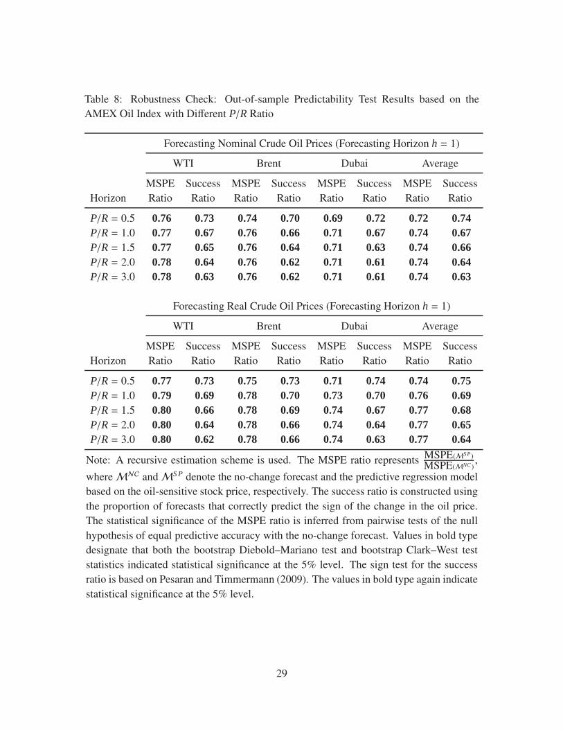
Table 8: Robustness Check: Out-of-sample Predictability Test Results based on the

AMEX Oil Index with Different P/R Ratio





P/R = 0.5 0.76 0.73 0.74 0.70 0.69 0.72 0.72 0.74P/R = 1.0 0.77 0.67 0.76 0.66 0.71 0.67 0.74 0.67P/R = 1.5 0.77 0.65 0.76 0.64 0.71 0.63 0.74 0.66P/R = 2.0 0.78 0.64 0.76 0.62 0.71 0.61 0.74 0.64P/R = 3.0 0.78 0.63 0.76 0.62 0.71 0.61 0.74 0.63





P/R = 0.5 0.77 0.73 0.75 0.73 0.71 0.74 0.74 0.75P/R = 1.0 0.79 0.69 0.78 0.70 0.73 0.70 0.76 0.69P/R = 1.5 0.80 0.66 0.78 0.69 0.74 0.67 0.77 0.68P/R = 2.0 0.80 0.64 0.78 0.66 0.74 0.64 0.77 0.65P/R = 3.0 0.80 0.62 0.78 0.66 0.74 0.63 0.77 0.64

Note: A recursive estimation scheme is used. The MSPE ratio represents MSPE(MS P)

MSPE(MNC ),

whereMNC andMS P denote the no-change forecast and the predictive regression model

based on the oil-sensitive stock price, respectively. The success ratio is constructed using

the proportion of forecasts that correctly predict the sign of the change in the oil price.

The statistical significance of the MSPE ratio is inferred from pairwise tests of the null

hypothesis of equal predictive accuracy with the no-change forecast. Values in bold type

designate that both the bootstrap Diebold–Mariano test and bootstrap Clark–West test

statistics indicated statistical significance at the 5% level. The sign test for the success

ratio is based on Pesaran and Timmermann (2009). The values in bold type again indicate

statistical significance at the 5% level.

29

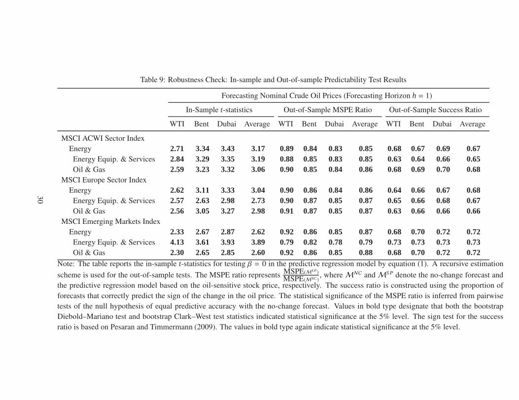
Table 9: Robustness Check: In-sample and Out-of-sample Predictability Test Results


In-Sample t-statistics Out-of-Sample MSPE Ratio Out-of-Sample Success Ratio

WTI Bent Dubai Average WTI Bent Dubai Average WTI Bent Dubai Average

MSCI ACWI Sector Index

Energy 2.71 3.34 3.43 3.17 0.89 0.84 0.83 0.85 0.68 0.67 0.69 0.67Energy Equip. & Services 2.84 3.29 3.35 3.19 0.88 0.85 0.83 0.85 0.63 0.64 0.66 0.65Oil & Gas 2.59 3.23 3.32 3.06 0.90 0.85 0.84 0.86 0.68 0.69 0.70 0.68

MSCI Europe Sector Index


MSCI Emerging Markets Index


Note: The table reports the in-sample t-statistics for testing β = 0 in the predictive regression model by equation (1). A recursive estimation

scheme is used for the out-of-sample tests. The MSPE ratio represents MSPE(MS P)

MSPE(MNC ), whereMNC andMS P denote the no-change forecast and

the predictive regression model based on the oil-sensitive stock price, respectively. The success ratio is constructed using the proportion of

forecasts that correctly predict the sign of the change in the oil price. The statistical significance of the MSPE ratio is inferred from pairwise

tests of the null hypothesis of equal predictive accuracy with the no-change forecast. Values in bold type designate that both the bootstrap

Diebold–Mariano test and bootstrap Clark–West test statistics indicated statistical significance at the 5% level. The sign test for the success

ratio is based on Pesaran and Timmermann (2009). The values in bold type again indicate statistical significance at the 5% level.

30

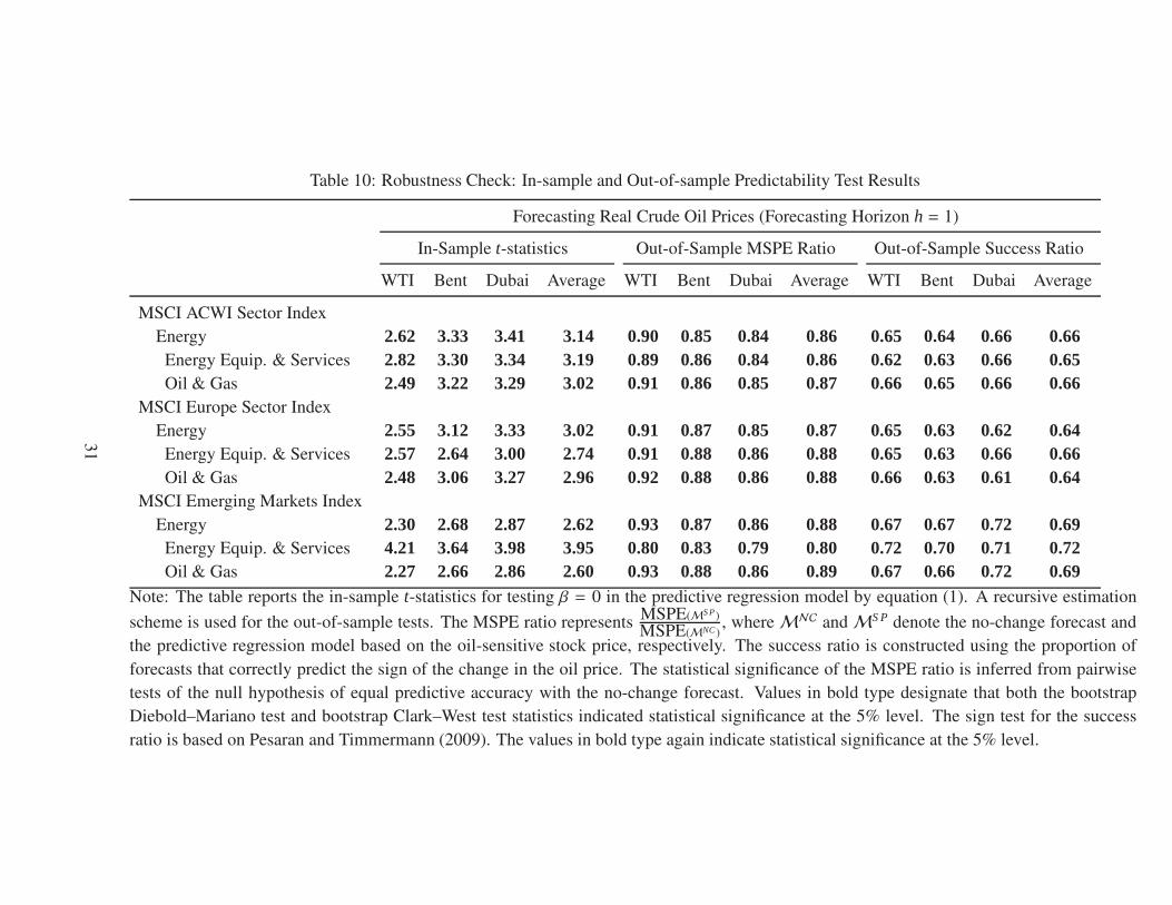
Table 10: Robustness Check: In-sample and Out-of-sample Predictability Test Results


In-Sample t-statistics Out-of-Sample MSPE Ratio Out-of-Sample Success Ratio

WTI Bent Dubai Average WTI Bent Dubai Average WTI Bent Dubai Average

MSCI ACWI Sector Index


MSCI Europe Sector Index


MSCI Emerging Markets Index


Note: The table reports the in-sample t-statistics for testing β = 0 in the predictive regression model by equation (1). A recursive estimation

scheme is used for the out-of-sample tests. The MSPE ratio represents MSPE(MS P)

MSPE(MNC ), whereMNC andMS P denote the no-change forecast and

the predictive regression model based on the oil-sensitive stock price, respectively. The success ratio is constructed using the proportion of

forecasts that correctly predict the sign of the change in the oil price. The statistical significance of the MSPE ratio is inferred from pairwise

tests of the null hypothesis of equal predictive accuracy with the no-change forecast. Values in bold type designate that both the bootstrap

Diebold–Mariano test and bootstrap Clark–West test statistics indicated statistical significance at the 5% level. The sign test for the success

ratio is based on Pesaran and Timmermann (2009). The values in bold type again indicate statistical significance at the 5% level.

31

0

20

40

60

80

100

120

140

84 86 88 90 92 94 96 98 00 02 04 06 08 10 12

WTI Brent Dubai

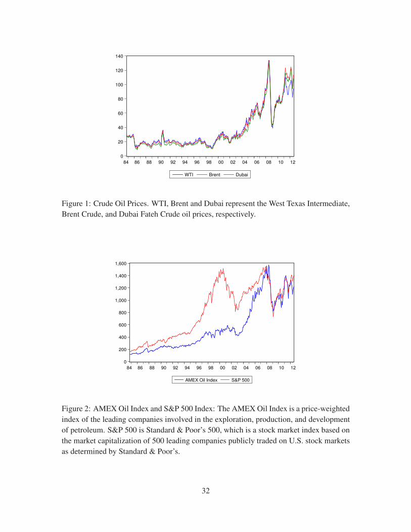
Figure 1: Crude Oil Prices. WTI, Brent and Dubai represent the West Texas Intermediate,

Brent Crude, and Dubai Fateh Crude oil prices, respectively.

0

200

400

600

800

1,000

1,200

1,400

1,600

84 86 88 90 92 94 96 98 00 02 04 06 08 10 12

AMEX Oil Index S&P 500

Figure 2: AMEX Oil Index and S&P 500 Index: The AMEX Oil Index is a price-weighted

index of the leading companies involved in the exploration, production, and development

of petroleum. S&P 500 is Standard & Poor’s 500, which is a stock market index based on

the market capitalization of 500 leading companies publicly traded on U.S. stock markets

as determined by Standard & Poor’s.

32

50

100

150

200

250

300

350

95 96 97 98 99 00 01 02 03 04 05 06 07 08 09 10 11 12

MSCI World Energy

60

80

100

120

140

160

180

200

95 96 97 98 99 00 01 02 03 04 05 06 07 08 09 10 11 12

MSCI World Transportation

40

60

80

100

120

140

160

95 96 97 98 99 00 01 02 03 04 05 06 07 08 09 10 11 12

MSCI World Air Freight & Logistics

60

80

100

120

140

160

95 96 97 98 99 00 01 02 03 04 05 06 07 08 09 10 11 12

MSCI World Airlines

0

100

200

300

400

500

95 96 97 98 99 00 01 02 03 04 05 06 07 08 09 10 11 12

MSCI World Energy Equipment & Services

0

100

200

300

400

500

95 96 97 98 99 00 01 02 03 04 05 06 07 08 09 10 11 12

MSCI World Marine

50

100

150

200

250

300

350

95 96 97 98 99 00 01 02 03 04 05 06 07 08 09 10 11 12

MSCI World Oil & Gas

40

80

120

160

200

240

95 96 97 98 99 00 01 02 03 04 05 06 07 08 09 10 11 12

MSCI World Road & Rail

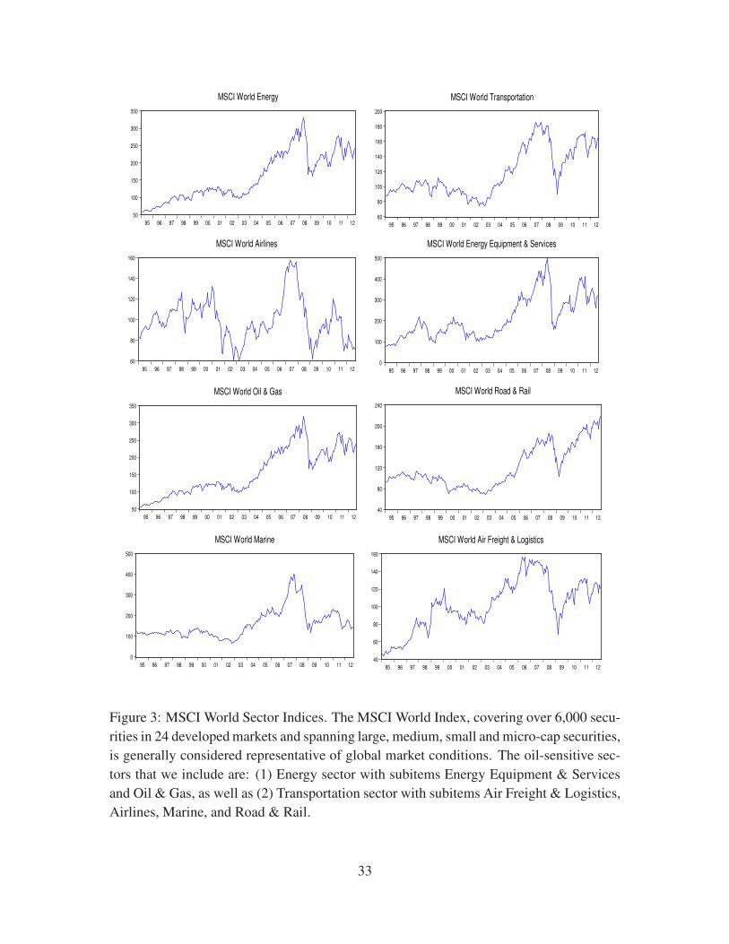
Figure 3: MSCI World Sector Indices. The MSCI World Index, covering over 6,000 secu-

rities in 24 developed markets and spanning large, medium, small and micro-cap securities,

is generally considered representative of global market conditions. The oil-sensitive sec-

tors that we include are: (1) Energy sector with subitems Energy Equipment & Services

and Oil & Gas, as well as (2) Transportation sector with subitems Air Freight & Logistics,

Airlines, Marine, and Road & Rail.

33

Documents

Forecasting Crude Oil Price Movements with Oil-Sensitive