Rm

Aa

b

c

ARRAA

KCRSSM

1

nevaKrf

1

(sorscss

w

0h

Computers and Chemical Engineering 55 (2013) 134– 147

Contents lists available at SciVerse ScienceDirect

Computers and Chemical Engineering

jo u r n al homep age : www.els evier .com/ locate /compchemeng

efinery scheduling of crude oil unloading with tank inventoryanagement

minu A. Hamisua, Stephen Kabantiokb, Meihong Wangc,∗

Process systems Engineering Group, School of Engineering, Cranfield University, MK43 0AL, UKWarri Refining and Petrochemical Company Limited, P.M.B. 44, Effurun, NigeriaDepartment of Engineering, University of Hull, Hull HU6 7RX, UK

a r t i c l e i n f o

rticle history:eceived 10 May 2012eceived in revised form 26 February 2013ccepted 2 April 2013vailable online xxx

a b s t r a c t

The aim of this study is to develop a methodology for short-term crude oil unloading, tank inventorymanagement, and crude distillation unit (CDU) charging schedule using mixed integer linear program-ming (MILP) optimization model as an extension to a previous work reported by Lee et al. (1996). Theauthors attempt to improve the previous model by adding an interval–interval variation constraint toavoid CDU charging rate fluctuation, a shutdown penalty within the scheduling cycle and a set up penalty

eywords:rude oilefinerychedulinghort-term operationixed-integer linear programming (MILP)

for tank-tank transfer and introducing demand violation permit for a more flexible model against obtain-ing infeasible solution. Three different cases from the original paper were used to test the validity of theimproved model. Comparison between Cases 1 and 2 shows the advantage of using smaller time intervalas the operating cost of Case 2 is lower. Two scenarios were created from Case 3 to show the benefits ofthe improved model in deciding the best schedule to use. The improved model was implemented usingthe CPLEX solver in GAMS.

. Introduction

The processing of crude oil into useful petroleum productsecessitates the establishment of a refining industry. This how-ver is of serious concern to the refiner considering high andolatile crude oil prices, environmental legislation, crude oilnd products quality, market demand and overall profit (Li, Li,arimi, & Srinivasan, 2007). In order to overcome these challenges,esearchers work towards developing computational algorithmsor crude oil scheduling.

.1. Scheduling and optimization of crude oil operation

Crude oil scheduling is a crucial part of the refinery supply chainSaharidis, Minoux, & Dallery, 2009). It is a process that involvespecifying the timing and sequence of operations in this orderf vessel arrival, crude oil unloading to storage tanks, transfer-ing crude oil from storage tanks to charging tanks and finallyent the mixed crude oil to crude distillation units (CDUs) for

omponent separations and downstream processing. A typicalchedule sets daily targets for production with consideration ontorage and charging tanks’ capacities, CDU capacity utilization and

∗ Corresponding author. Tel.: +44 (0)1482 466688.E-mail addresses: Meihong.Wang@hull.ac.uk,

ang 2003 uk@yahoo.co.uk (M. Wang).

098-1354/$ – see front matter © 2013 Elsevier Ltd. All rights reserved.ttp://dx.doi.org/10.1016/j.compchemeng.2013.04.003

© 2013 Elsevier Ltd. All rights reserved.

pumping capabilities. It also determines the quality and quantityof crude mixing materials in the charging tanks in order to produceblends that satisfy the requirements of planning team. Each of theseactivities is associated with cost. The objective of scheduling is tominimize the total cost while following the feasible operationalprocedures (Jia, Ierapetritou, & Kelly, 2003).

In research studies, refinery scheduling problems are often pre-sented as optimization model with operating cost as the objectivefunction. The challenge with building models for scheduling liesin knowing and including what is relevant for the specific deci-sions that are to be made using the model and neglecting theelements that are not relevant. Selection of units with arrangmentson the sequence of operation with regards to modelling of refineryscheduling problems require a systematic approach. Optimizationtechniques are used extensively in this area of study to come upwith schedules that are not only acceptable to the planning teambut also to the satisfaction of the customers adequately.

1.2. Recent progress in refinery scheduling

Significant progress has been made over the years in sched-uling of crude oil unloading, mixing and charging of the CDU.

The trend involves using mathematical models with constraintsand bounds on the stream connections. A number of researcherspresented problems with continuous and discrete decisions forcrude oil scheduling. For instance, the work of Bassett, Pekny,

A.A. Hamisu et al. / Computers and Chemical Engineering 55 (2013) 134– 147 135

Nomenclature

Subscriptsj charging tanki storage tankg other charging tankk key componentl crude distillation unitm other time intervalt time intervalv crude oil vesselo initial value

ParametersCC charging tanks changeover costCINBTj charging tanks j inventory cost per unit time per unit

volumeCINSTi storage tanks i inventory cost per unit time per unit

volumeCS cost penalty for shutdownCSEAv sea waiting cost for vessel vCSSU cost penalty for switching to another tank during

tank-tank transfersCOPR operating costCUNLv unloading cost for vessel vDj,l,t binary variable that denotes charging tank j is charg-

ing CDU l at time interval tDg,l,t binary variable that denotes charging tank g is

charging CDU l at time interval tDMq demand of crude mix qNBT number of charging tanksNCDU number of CDUsNCOMP number of key componentsNST number of storage tanksNSCH number of time intervals in scheduling horizonNV number of vesselsTARRv arrival time of vessel vTFv time vessel v begins to unloadTLv time vessel v finishes unloadingε1q violation parameter due to decrease in demandε2q violation parameter due to increase in demand�l user defined parameter that determines

interval–interval variations for CDU l throughput

Variablesfbcj,l,k,t volumetric flow rate of component k from charging

tank j to CDU l at time tfsbi,j,k,t volumetric flow rate of component k from storage

tank i to charging tank j at time tf vsv,i,k,t volumetric flow rate of component k from vessel v

to storage tank i at time tFBCj,l,t volumetric flow rate from charging tank j to CDU l

at time tFBCmaxj,l maximum volumetric flow rate from charging

tank j to CDU lFBCminj,l minimum volumetric flow rate from charging tank

j to CDU lFSBi,j,t volumetric flow rate from storage tank i to charging

tank j at time tFSBmaxi,j maximum volumetric flow rate from storage tank

i to charging tank jFSBmini,j minimum volumetric flow rate from storage tank i

FVSmaxv,i maximum volumetric flow rate from vessel v tostorage tank i

FVSminv,i minimum volumetric flow rate from vessel v tostorage tank i

vbj,k,t volume of component k in charging tank j at time tvsi,k,t volume of component k in storage tank i at time tVBj,t volume of charging tank j at time tVBmaxj maximum volume of charging tank jVBminj minimum volume of charging tank jVSi,t volume of storage tank i at time tVSmaxi maximum volume of storage tank iVSmini minimum volume of storage tank iVVv,t volume of crude oil vessel v at time twsi,k concentration of component k in storage tank iwsmaxi,k maximum concentration of component k in stor-

age tank iwsmini,k minimum concentration of component k in storage

tank iwbj,k concentration of component k in charging tank jwbmaxj,k maximum concentration of component k in charg-

ing tank jwbminj,k minimum concentration of component k in charg-

ing tank jwvv,k concentration of component k in crude oil vessel vXDl,t binary variable that indicates shutdown of CDU l at

time tXFv,t binary variable that denotes that vessel v starts

unloading at time tXLv,t binary variable that denotes that vessel v stops

unloading at time tXWv,t binary variable that denotes that vessel v is unload-

ing to storage tank i at time tXWSi,j,t binary variable that denotes that storage tank i is

transferring charging tank j at time tZj,l,t binary variable that denotes that charging tank j

charges the CDU l at time tZj,g,l,t binary variable that denotes that CDU l switched

from charging tank j to charging tank g at time t˛i,t binary variable that denotes that storage i tank is set

up for tank-tank transfer

to charging tank jFVSv,i,t volumetric flow rate from vessel v to storage tank i

at time t

and Reklaitis (1996) that considers a model based approach toaddress a large-scale scheduling problem while considering lengthof the scheduling horizon (time), the number of units/equipmentinvolved and the number of operations and available resources.Since scheduling of crude oil operations usually involves con-tinuous and discrete decisions, MILP is used in formulating thescheduling problems.

Two popular approaches based on time representation of thescheduling horizon have been used in formulating MILP: discrete-time formulation and continuous-time formulation. A third butless popular approach combines these two time formulations todevelop mixed time formulation (Westerlund, Hastbacka, Forssell,& Westerlund, 2007). Mouret, Grossmann, and Pestiaux (2009)introduced a new approach for continuous-time formulationknown as priority-slot based method. Pinto, Joly, and Moro (2000)used variable length time slot for creating short-term scheduling ofcrude oil operations in a 200,000 bpd refinery that receives aboutten different crude types in seven storage tanks. They used uni-

form time discretization of 15 min to generate an MILP problemthat could not be solved with the available optimization technologyat that time.

1 hemi

boatspfttgurf

fesptamp(codrcs

lGlgogewtis

1

iauo&oucurdmauoib

mt

36 A.A. Hamisu et al. / Computers and C

Lee et al. (1996) used a mixed integer optimization modelased on uniform time discretization for short-term schedulingf crude oil unloading with inventory management. Shah, Li,nd Ierapetritou (1996) adopted a mathematical programmingechnique to develop a model for a single refinery consisting ofcheduled ship arrivals, port infrastructure, pipeline details, androduction requirements and planned CDU runs, based on uni-orm time discretization with the objective of minimizing theank heels. Yee and Shah (1998) used two methods to tightenhe relaxation gap and narrow down the search space for inte-er solution of scheduling problem in a multipurpose plant. These of time discretization presents some challenges making otheresearchers to seek for more possible options such as events-basedormulations.

Saharidis et al. (2009) presented MILP formulation with uni-orm discrete-time intervals where the intervals are based onvents instead of hours. Jia et al. (2003) developed a model forcheduling of oil refinery operations based on unit specific eventoint formulation using the state task network (STN) representa-ion introduced by Kondili, Pantelides, and Sargent (1993). Morond Pinto (2004) developed a global events-based continuous-timeodel for crude oil inventory management of a refinery which

rocesses several types of crude oil. Saharidis and Ierapetritou2009) used an event-based time formulation for scheduling ofrude oil unloading, storage and charging of CDUs. The goalf their model was to optimize crude oil blending and cutown the number of tank setup during vessel unloading therebyeducing the number of tanks used. Simplification of a complexase to problems of manageable size is an incentive in refinerycheduling.

Several authors have adopted an approach that breaks downarge scheduling problems into smaller problems. Harjunkoski androssmann (2001) used a spatial decomposition strategy to split

arge scheduling problem for steel production into smaller pro-rammes. This method produced solution within 1–3% of the globalptimum. Shah, Saharidis, Jia, and Ierapetritou (2009) presented aeneral novel decomposition scheme which breaks down the refin-ry scheduling problem spatially into subsystems. The subsystemsere solved to optimality and the optimal results were integrated

o obtain the optimal solution for the entire problem. This resultn fewer continuous and binary variables compared to centralizedystems.

.3. Motivations, aim and objectives and novelties of this paper

Optimization of petroleum refining processes promises a big cutn operational and logistic costs. Better economic performance arechieved by employing robust procedures for short-term sched-ling of material flow. Despite these benefits, there is still a gapf knowledge that needs to be filled in this niche (Wu, Chu, Chu,

Zhou, 2011). Lee et al. (1996) addresses the problem of crudeil unloading, inventory management and the charging schedulessing discrete-time formulation, their model failed to incorporateertain details to reflect real industrial practices. For instance, thencontrolled fluctuation of CDU feed rate; which in one instanceesulted in a 10:1 turndown ratio. Although Li et al. (2007) haveone a good job towards addressing nonlinearity in schedulingodel; their solution is still a tradeoff between feasibility and

ccuracy and their procedure does not include violation in prod-ct demand. Yüzgec , Palazoglu, and Romagnoli (2010) did overlookther events happening beyond the scheduling horizon such as fix-ng closing stocks. Overcoming these challenges is the motivation

ehind this paper.

Therefore this paper is aimed at improving Lee et al. (1996) MILPodel making it more robust and reflects real industrial applica-

ions. The modifications considered for the improvement are:

cal Engineering 55 (2013) 134– 147

• Interval–interval volume variation constraint is added; this pre-vents widely fluctuating CDU charging rate.

• A CDU shutdown penalty is added rather than the hard con-straint that mandates CDUs to be operational throughout thehorizon. The improved model considered the possibility of shut-down within the scheduling cycle.

• A setup penalty for tank-tank transfer is included in Case 3.• Some level of flexibility is introduced so that demand violation is

permitted when exact demand constraints leads to infeasibility(Case 3: scenario A).

• The standing gauge constraint is applied not only when charg-ing tank feeds CDU but also during transfer from storage tank tocharging tank.

• The improved model permits fixing of closing stocks within thescheduling cycle (Case 3).

1.4. Outline of the paper

A modification of the problem statement alongside the mathe-matical formulation of the improved model is presented in Section2. The validity of the improved model was tested using cases fromLee et al. (1996) and the results are presented in Section 3. The vali-dation was accomplished by implementing the improved model inthe general algebraic modelling system (GAMS) code for each caseto account for their individual peculiarity. Section 4 presents thesimulation results of the improved model for a typical industry sizeproblem. Section 5 is a summary of the whole paper based on theresults from Sections 3 and 4.

2. Model formulation and problem definition

Same as in Lee et al. (1996), this paper considers a coastalrefinery with docking stations where the crude vessels unloadtheir content; storage tanks for holding crude oil before trans-fer to charging tanks; charging tanks where blending operation iscarried out for subsequent transfer to CDUs in accordance withthe CDUs crude mix quality requirements. These tranfer opera-tions are achieved in different units/facilities interconnected bymeans of a pipe network. Throughout the scheduling horizon,industry operational practice is observed. The following infor-mation are included in most of petroleum refinery schedulingproblems.

• Number of vessels, amount and crude oil type conveyed and thearrival and departure times of each vessel.

• Number of units/facilities for the crude oil transfer from vesseldown to the CDU with their capacity limits, initial inventory levelsand interconnections.

• Upper and lower bounds on the stream flows across the connect-ing units/facilities.

• Specification of key components with their permissible concen-tration ranges.

• Information on dedication of certain tanks for receiving only par-ticular types of crude.

• Other information such as CDUs demand of blended crude fromcharging tanks, unloading and sea waiting costs of vessels,inventory costs for charging and storage tanks, changeover andshutdown costs for CDUs.

2.1. Problem definition

With the information above and the improved model, the sched-uling problem is to minimize the overall cost of operation bydetermining the following optimization variables:

hemi

••••

•

•••

•

acdsr

2

2

Rt

1

2

3

4

5

2

wscsm

C

A.A. Hamisu et al. / Computers and C

Waiting time for each vessel until the unloading process begins.Unloading duration for each vessel.Volume per unit time of crude oil unloaded for each vessel.Volume per unit time of crude oil transferred from vessels tostorage tanks then to charging tanks and finally to CDUs.Vessels, storage and charging tanks inventory levels at each timeinterval within the scheduling horizon.CDU charging rates.Time and sequence of charging of mixed crude into each CDU.Time and sequence of crude transfer from storage to chargingtank.Concentration of key component (such as sulphur) in chargingtank.

The improved model is formulated based on established oper-ting rules, material balance constraints, resources allocationonstraints, sequence constraints, product quality and crude oil mixemand constraints. Kelly and Mann (2003) classified these con-traints into three major groups: hydraulic capacities, operatingules, and property specifications.

.2. Mathematical model formulation

.2.1. Model assumptionsSame as in Lee et al. (1996), Li et al. (2007), Yüzgec et al. (2010),

eddy, Karimi, and Srinivasan (2003) and Pan, Li, and Qian (2009);he following assumptions are considered in this paper.

. The unloading operation is carried out in only one dockingstation.

. Volume of crude oil remaining in the pipeline is negligible com-pared to the total volume processed in the entire schedulinghorizon.

. The time for change-over is negligible compared to the entirescheduling horizon.

. Perfect mixing occurs in the charging tank and mixing time isnegligible.

. Continuous demand order matches the limits of the CDU opera-tions.

.2.2. Objective functionThe objective function is the cost function to be minimized,

hich includes unloading and sea waiting costs for the crude ves-els, the storage and charging tanks inventory costs, changeoverost and the penalties for shutdown and tank-tank transfer. Thehutdown penalty and the tank-tank set-up penalty newly addedakes the cost function different from that in Lee et al. (1996).

OPR = CUNLv

NV∑v=1

(TLv − TFv) + CSEAv

NV∑v=1

(TFv − TARRv)

+ CINSTi

NST∑i=1

NSCH∑t=1

(VSi,t + VSi,t−1

2

)

NBT NSCH ( )

+CINBTj

∑j=1

∑t=1

VBj,t + VBj,t−1

2

+NSCH∑t=1

NBT∑j=1

NCDU∑l=1

(CC × Zj,l,t) +NSCH∑t=1

NCDU∑l=1

(CS × XDl,t) (1)

cal Engineering 55 (2013) 134– 147 137

2.2.3. Constraints2.2.3.1. Operating rules.

1. Vessel unloading sequence:a. Vessel arrives and leaves the docking station only once

throughout the scheduling horizon.

NSCH∑t=1

XFv,t = 1 v = 1, . . . , NV (2)

NSCH∑t=1

XLv,t = 1 v = 1, . . . , NV (3)

b. A vessel can only unload after it arrives at the docking stationas determined at the planning level.

TFv ≥ TARR,v v = 1, . . . , NV (4)

c. The initiation and completion times are defined as:

TFv =NSCH∑t=1

tXFv,t v = 1, . . . , NV (5)

TLv =NSCH∑t=1

tXLv,t v = 1, . . . , NV (6)

d. Based on the assumption that there is only one dockingstation, two vessels cannot unload their contents at the sametime. Therefore the preceding vessel must finish unloadingone time interval before the later vessel begins to unload.

TFv+1 ≥ TLv + 1 v = 1, . . . , NV (7)

e. A vessel unloading is accomplished between two time inter-vals: initiation time, TFv and completion time, TLv

XWv,t ≤t∑

m=1

XFv,m, XWv,t ≤NSCH∑m=t

XLv,m (8)

v = 1, . . . , NV, t = 1, . . . , NSCHf. The unloading duration is bounded by TFv and TLv.

TLv − TFv ≥ 1 v = 1, . . . , NV (9)

2. Standing gauge operation: flow in and out of tanks simulta-neously is not allowed.a. For storage tanks:

XWSi,j,t ≤ 1 − XWv,i,t (10)

v = 1, . . . , NV, i = 1, . . . , NST, j = 1, . . . , NBT,

t = 1, . . . , NSCH

b. For charging tanks:

Dj,l,t ≤ 1 − XWSi,j,t (11)

i = 1, . . . , NST, j = 1, . . . , NBT, l = 1, . . . , NCDU,

t = 1, . . . , NSCH

3. Semi-continuous constraints are applied for feedstock to CDU;these ensure operation of the unit within the design flow rateand assumes no flow when CDU shut down.

1 hemi

38 A.A. Hamisu et al. / Computers and C

For normal operation the constraint is represented as:

FBCminj,l ≤ FBCj,l,t ≤ FBCmaxj,l (12)

j = 1, . . . , NBT, l = 1, . . . , NCDU, t = 1, . . . , NSCH

When CDU shuts down,

FBCj,l,t = 0 (13)

j = 1, . . . , NBT, l = 1, . . . , NCDU, t = 1, . . . , NSCH

4. Flow constraint from storage tank to charging tank: for multiplestorage tanks feeding charging tank (s), a pipeline can only belined up to just one charging tank at a time. The total quantityreceived by charging tank (s) must not exceed the maximumflow rate from storage tanks. For connecting pipeline betweenstorage and charging tanks when storage tanks are unloadingthe constraint is represented as:

NST∑i

FSBi,j,t ≤ FSBmaxi,j (14)

i = 1, . . . , NST, j = 1, . . . , NBT, t = 1, . . . , NSCH

5. Demand violation constraints: unlike in Lee et al. (1996) a vio-lation in demand order is introduced here to make the modelmore flexible. This is necessary because the model becomesinfeasible where supply failed to meet the exact demand. Fordemand of crude oil mix q from charging tank j, Eq. (15) rep-resents supply to meet exact or below actual demand and Eq.(16) to account for supply to meet the exact or above actualdemand.NCDU∑

l=1

NSCH∑t=1

FBCj,l,t ≥ DMq(1 − ε1q) (15)

j = 1, . . . , NBT, q = 1, . . . , NBT

andNCDU∑

l=1

NSCH∑t=1

FBCj,l,t ≤ DMq(1 − ε1q) (16)

j = 1, . . . , NBT, q = 1, . . . , NBT

ε1q is a parameter that specifies the demand violation of crudemix q in the negative direction (below the actual demand) andε2q specifies the demand violation of crude mix q in the posi-tive direction (above the actual demand). When each of theseparameters is 0, a demand violation is not allowed and when itis 1, a 100% violation in demand order is allowed. With theseparameters, it is possible to carry out a sensitivity analysis todetermine the maximum value of demand violation of eachcrude mix that will maintain the optimal solution of the MILPscheduling model.

6. Continuous flow constraint: at any time, one charging tankshould be charging the CDU.

NBT∑D = 1 (17)

j

j,l,t

l = 1, . . . , NCDU, t = 1, . . . , NSCH

cal Engineering 55 (2013) 134– 147

7. Flow fluctuation constraints: widely varying interval–intervalCDUs charging rate should be avoided because it disrupts CDUoperation and may generate off specification cuts. Two con-straints are imposed to limit the interval–interval variation inquantity fed to the CDU. These are:

FBCj,l,t−1 ≥ FBCj,l,t(1 − �l) (18)

j = 1, . . . , NBT, l = 1, . . . , NCDU, t = 1, . . . , NSCH − 1

and

FBCj,l,t−1 ≤ FBCj,l,t(1 + �l) (19)

j = 1, . . . , NBT, l = 1, . . . , NCDU, t = 1, . . . , NSCH − 1

�l is a user defined parameter with values ranging betweenzero and one. If �l is set at zero, no variation in interval–intervalquantity while setting it to 1 implies that 100% variation is per-mitted. For the cases in this paper a conservative value of 0.1 isused.

8. Changeover penalty: this is to consider a cost associated withswitching of charging tanks any time it occurs. Lee et al. (1996)represents changeover as a point when a charging tank j at timet − 1 charges the CDU followed by another charging tank g at alater time t.

Zj,g,l,t ≥ Dg,l,t + Dj,l,t−1 − 1 (20)

j, g(j /= g) = 1, . . . , NBT, l = 1, . . . , NCDU,

t = 1, . . . , NSCH − 1

Eq. (20) results in a large number of integer variables andconstraints, making it computationally expensive for problemsinvolving multiple CDUs. An improvement over this by Li, Hui,Hua, and Tong (2002) overcomes the challenge by reducing thechangeover penalty variable Zj,g,l,t from a tetra-indexed variableto a tri-index variable Zj,l,t. A simple approach adopted in theirpaper suggests the use of Eqs. (21) and (22).

Zj,l,t ≥ Dj,l,t − Dj,l,t−1 (21)

j = 1, . . . , NBT, l = 1, . . . , NCDU, t = 1, . . . , NSCH − 1

Zj,l,t ≥ Dj,l,t−1 − Dj,l,t (22)

j = 1, . . . , NBT, l = 1, . . . , NCDU, t = 1, . . . , NSCH − 1

The term CC × Zj,l,t is added to the objective function CC is thecost penalty for changeover.

9. Shutdown constraints: these are included to permit generat-ing flexible schedules involving both shutdown and continualoperations. Thus,

FBCj,l,t ≥ (1 − XDl,t)FBCloj,l,t (23)

j = 1, . . . , NBT, l = 1, . . . , NCDU, t = 1, . . . , NSCH − 1

FBC ≤ (1 − XD )FBCup (24)

j,l,t l,t j,l,t

j = 1, . . . , NBT, l = 1, . . . , NCDU, t = 1, . . . , NSCH − 1

hemi

1

2

1

2

3

A.A. Hamisu et al. / Computers and C

The binary variable XDl,t is zero during normal operation andtakes on the value of 1 when CDU shuts down. The minimumflow rate threshold before CDU deemed to have shutdown,FBCloj,l,t is the lower bound on the flow FBC with FBCupj,l,t beingthe upper bound. The term CS × XDl,t is added to the objectivefunction. CS is the cost penalty for shutdown.

0. Set-up constraint: in real life situation, tank-tank tranferinvolve some activities when a crude vessel is allowed tounload into multiple storage tanks for subsequent transfer ofthe crude oil into charging tanks. A set-up cost is incurredanytime switching occurs between storage tanks and chargingtanks. Including a set-up cost for these activities in the objectivefunction minimizes the number of these activities.

˛i,t ≥ XWSi,j,t − XWSi,j,t−1 (25)

i = 1, . . . , NST, j = 1, . . . , NBT, t = 1, . . . , NSCH − 1

This set-up cost is considered in Case 3 (Example 4 in Lee et al.(1996)) with more storage and charging tanks translating intoa quite number of switchover operations. The term CSSU × ˛i,tis added to the objective function for this case. CSSU is thecost penalty for switching from tank to tank during tank-tanktransfers.

.2.3.2. Hydraulic capacities (Lee et al., 1996).

. Flow constraints: flow of the crude oil is bounded by the capacityof the pumping system available. For the main units/facilities forcrude oil transfer, the following holds:a. Flow from vessel to storage tank

FVSminv,iXWv,i,t ≤ FVSv,i,t ≤ FVSmaxv,iXWv,i,t (26)

v = 1, . . . , NV, i = 1, . . . , NST, t = 1, . . . , NSCHb. Flow from storage tank to charging tank

FSBmini,jXWSi,j,t ≤ FSBi,j,t ≤ FSBmaxi,jXWSi,j,t (27)

i = 1, . . . , NST, j = 1, . . . , NBT, t = 1, . . . , NSCHc. Flow from charging tank to CDU.

FBCminj,lDj,l,t ≤ FBCj,l,t ≤ FBCmaxj,lDj,l,t (28)

j = 1, . . . , NBT, l = 1, . . . , NCDU, t = 1, . . . , NSCH. Capacity constraints: the volume of crude oil in storage and

charging tanks at any time must be within the upper and lowerbounds of the containing medium.a. Storage tank capacity limitation.

VSmini ≤ VSi,t ≤ VSmaxi (29)

i = 1, . . . , NST, t = 1, . . . , NSCHb. Charging tank capacity limitation.

VBminj ≤ VBj,t ≤ VBmaxj (30)

j = 1, . . . , NBT, t = 1, . . . , NSCH. Crude oil material balance.

a. Crude oil vessel: volume of crude oil in vessel v at time t equalsthe difference between the initial crude volume and the over-all volume transferred from the vessel up to time t.

NST∑ t∑

VVv,t = VVv,0 −

i=1 m=1

FVSv,i,m (31)

v = 1, . . . , NV, t = 1, . . . , NSCH

cal Engineering 55 (2013) 134– 147 139

For the whole scheduling horizon, the equation becomes:

VVv,0 =NST∑i=1

NSCH∑t=1

FVSv,i,t (32)

v = 1, . . . , NVAt any time period within the scheduling horizon, the fol-

lowing equation holds for crude oil vessels.

FVSv,i,t ≤ VVv,t (33)

v = 1, . . . , NV, i = 1, . . . , NST, t = 1, . . . , NSCHb. Storage tank: volume of crude oil in storage tank i at time t

equals the sum of the initial volume stored in the storage tankwith the volume transferred into the storage tank up to timet, less volume transferred from the storage tank up to time t.

VSi,t = VSi,0 +NV∑v=1

t∑m=1

FVSv,i,m −NBT∑j=1

t∑m=1

FSBi,j,m (34)

i = 1, . . . , NST, t = 1, . . . , NSCHAt any time period within the scheduling horizon, the fol-

lowing equation holds for storage tanks.

FSBi,j,t ≤ VSi,t (35)

i = 1, . . . , NST, j = 1, . . . , NBT, t = 1, . . . , NSCHc. Charging tank: volume of crude mix in charging tank j at time t

equals the sum of the initial volume of crude mix in the charg-ing tank with the volume transferred into the charging tankup to time t, less volume transferred from the charging tankup to time t.

VBj,t = VBj,0 +NST∑i=1

t∑m=1

FSBi,j,m −NCDU∑

l=1

t∑m=1

FBCj,l,m (36)

j = 1, . . . , NBT, t = 1, . . . , NSCHAt any time period within the scheduling horizon, the fol-

lowing equation holds for charging tanks.

FBCj,l,t ≤ VBj,t (37)

j = 1, . . . , NBT, l = 1, . . . , NCDU, t = 1, . . . , NSCH4. Component material balance. The component material balance

in storage tanks should only be used when there is mixing instorage tank due to difficulty in segregating crudes of differ-ent compositions. The mixing here is not the same as blendingoperation as the later is limited to charging tanks only.a. Storage tank: volume of component k in storage tank i at time

t equals the sum of volume of component k in the storage tankwith the volume of component k transferred into the storagetank up to time t, less volume of component k transferred fromthe storage tank up to time t.

vsk,i,t = vsk,i,0 +t∑

m=1

NV∑v=1

f vsk,v,i,m −t∑

m=1

NBT∑j=1

fsbk,i,j,m (38)

k = 1, . . . , NCOMP, i = 1, . . . , NST, t = 1, . . . , NSCHComponent volumetric flow from vessel to storage tank

f vsk,v,i,t = FVSv,i,twvk,v (39)

k = 1, . . . , NCOMP, v = 1, . . . , NV, i = 1, . . . , NST,

t = 1, . . . , NSCH

b. Charging tank: volume of component k in charging tank j attime t equals the sum of volume of component k in the charg-ing tank with the volume of component k transferred into

1 hemi

2

1

2

2

Hml

•

•

40 A.A. Hamisu et al. / Computers and C

the charging tank up to time t, less volume of component ktransferred from the charging tank up to time t.

vbk,j,t = vbk,j,0 +t∑

m=1

NST∑i=1

fsbk,i,j,m −t∑

m=1

NCDU∑l=1

fbck,j,l,m (40)

k = 1, . . . , NCOMP, j = 1, . . . , NBT, t = 1, . . . , NSCHComponent volumetric flow from storage tank to charging

tank

fsbk,i,j,t = FSBi,j,twsk,i (41)

k = 1, . . . , NCOMP, i = 1, . . . , NST, j = 1, . . . , NBT,

t = 1, . . . , NSCH

.2.3.3. Property specification.

. Component flow specification: the flow of key component fromone tank to the other has a limit (Lee et al., 1996).a. Component flow from storage to charging tank is bounded by

an upper and a lower limit.

wsmink,iFSBi,j,t ≤ fsbk,i,j,t ≤ wsmaxk,iFSBi,j,t (42)

k = 1, . . . , NCOMP, i = 1, . . . , NST, j = 1, . . . , NBT,

t = 1, . . . , NSCH

b. Component flow specification for flow from charging tank toCDU is

wbmink,jFBCj,l,t ≤ fbck,j,l,t ≤ wbmaxk,jFBCj,l,t (43)

k = 1, . . . , NCOMP, j = 1, . . . , NBT, l = 1, . . . , NCDU,

t = 1, . . . , NSCH

. Component volume limitation:a. Storage tank: the limit for the volume of component k in stor-

age tank at any time is

wsmink,iVSi,t ≤ vsk,i,t ≤ wsmaxk,iVSi,t (44)

k = 1, . . . , NCOMP, i = 1, . . . , NST, t = 1, . . . , NSCHb. Charging tank: the limit for the volume of component k in

charging tank at any time is

wbmink,jVBj,t ≤ vbk,j,t ≤ wsmaxk,jVBj,t (45)

k = 1, . . . , NCOMP, j = 1, . . . , NBT, t = 1, . . . , NSCH

.3. Summary of model improvements

This section highlights the main contributions of this paper.ere, the following constraints are included to come up with aore reliable MILP short-term scheduling model addressing a real

ife refinery operational issues.

Flow fluctuation constraints: these are added to preventinterval–interval variation of CDU charging rates. The constraintsare enforced using Eqs. (18) and (19). These constraints were notincluded in Lee et al. (1996) and as a result schedules generated

using their model produced unrealistic widely fluctuating CDUvolumetric rate.CDU shutdown constraints with penalty: because of the hugelosses associated with shutdown, it is highly undesirable and

cal Engineering 55 (2013) 134– 147

plants are for most times run continuously. However, in thispaper we consider constraints that allow generating schedulesthat include both shutdown and continual operations. The con-straints are represented by Eqs. (23) and (24). A shutdown penaltyis included in the objective function to minimize any cost associ-ated with the shutdown operation.

• Set-up constraint (Eq. (25)) with penalty: this is to optimize thenumber of activities prior to transfer from storage tanks to charg-ing tanks for a case involving unloading into multiple storagetanks and subsequent transfer of crude oil into multiple charg-ing tanks. The improved model schedules only important set-upsthereby minimizing the number of operations during tank-tanktransfers when a set-up penalty is included in the objective func-tion. This set-up constraint with penalty is considered in Case3.

• Demand violation constraints: unlike in Lee et al. (1996), viola-tion in demand order are introduced here to make the modelmore flexible. These are necessary because the model becomesinfeasible where supply failed to meet exact demand. These arerepresented by Eqs. (15) and (16) and incorporated in Case 3:Scenario A.

• Standing gauge constraints are applied not only when chargingtank feeds CDU but also during transfer from storage tanks tocharging tanks (Eqs. (10) and (11)). This is an industry practicewhich was not included in Lee et al. (1996).

• Of particular interest to the scheduler is making a forecast onevents happening beyond the actual time horizon in order tostudy uncertainty in the CDU demand order. The improved modelpermits fixing of closing stocks within the scheduling cycle,meaning that it gives room for generating schedules that can bestretched beyond the scheduling horizon by a day or two. The ideawas demonstrated in some of the cases studied in this paper.

3. Case studies

With the improved model, two case studies (Case 1 and Case2) from Lee et al. (1996) paper are discussed in this section. Case1 is the motivating example in the paper with 24hr discrete timeintervals spanning over 8 days. Case 2 is same as Case 1 but an 8hrinterval was considered. In this paper, the following recommen-dations were adopted when implementing the improved model inGAMS for the cases under study.

• Karri, Srinivasan, and Karimi (2009) and Li et al. (2002) recom-mended a flow fluctuation constraint that puts an upper andlower limits to the interval to interval fluctuations in crude oilprocessing rate. For all the cases considered in this paper (Case 1,Case 2 and industry size case study), a ceiling of 10% is fixed forflow variation while at the same time restricting the CDUs to runwithin the permissible minimum turndown ratio of 10:6.

• In consideration to the manner in which storage and chargingtanks are configured as floating roof objects in a refinery andthe volatile nature of crude oil, a minimum level of the fluid isalways maintained in those tanks for safety reasons. This papersuggests that a minimum level for all tanks be fixed at 100 kbbland a maximum value at 1100 kbbl. The difference between thesetwo values is in agreement with the volume difference used in Leeet al. (1996).

3.1. Case 1

The case study begins with the motivating example from Leeet al. (1996) to illustrate how the ideas proposed in this paper helpin achieving better and realistic results. Like Lee et al. (1996), thispaper considered a system comprises of one docking station, two

A.A. Hamisu et al. / Computers and Chemical Engineering 55 (2013) 134– 147 141

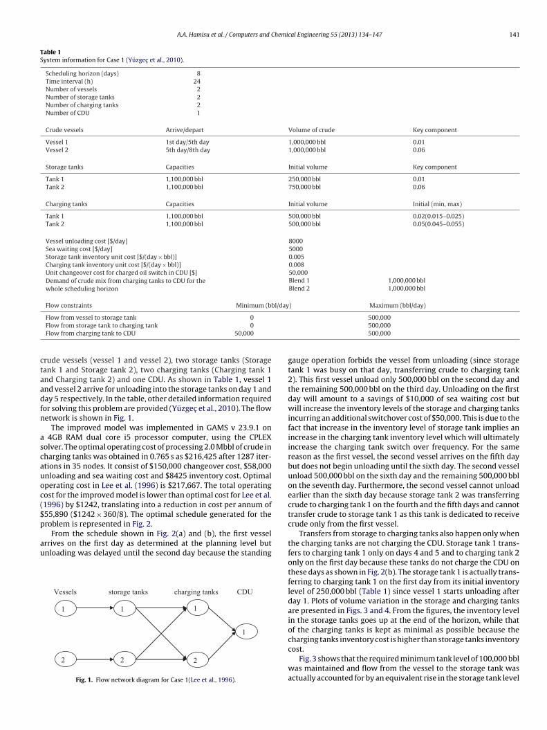
Table 1System information for Case 1 (Yüzgec et al., 2010).

Scheduling horizon (days) 8Time interval (h) 24Number of vessels 2Number of storage tanks 2Number of charging tanks 2Number of CDU 1

Crude vessels Arrive/depart Volume of crude Key component

Vessel 1 1st day/5th day 1,000,000 bbl 0.01Vessel 2 5th day/8th day 1,000,000 bbl 0.06

Storage tanks Capacities Initial volume Key component

Tank 1 1,100,000 bbl 250,000 bbl 0.01Tank 2 1,100,000 bbl 750,000 bbl 0.06

Charging tanks Capacities Initial volume Initial (min, max)

Tank 1 1,100,000 bbl 500,000 bbl 0.02(0.015–0.025)Tank 2 1,100,000 bbl 500,000 bbl 0.05(0.045–0.055)

Vessel unloading cost [$/day] 8000Sea waiting cost [$/day] 5000Storage tank inventory unit cost [$/(day × bbl)] 0.005Charging tank inventory unit cost [$/(day × bbl)] 0.008Unit changeover cost for charged oil switch in CDU [$] 50,000Demand of crude mix from charging tanks to CDU for thewhole scheduling horizon

Blend 1 1,000,000 bblBlend 2 1,000,000 bbl

Flow constraints Minimum (bbl/day) Maximum (bbl/day)

Flow from vessel to storage tank 0 500,000

ctaadfn

ascauoc($p

au

Flow from storage tank to charging tank 0

Flow from charging tank to CDU 50,000

rude vessels (vessel 1 and vessel 2), two storage tanks (Storageank 1 and Storage tank 2), two charging tanks (Charging tank 1nd Charging tank 2) and one CDU. As shown in Table 1, vessel 1nd vessel 2 arrive for unloading into the storage tanks on day 1 anday 5 respectively. In the table, other detailed information requiredor solving this problem are provided (Yüzgec et al., 2010). The flowetwork is shown in Fig. 1.

The improved model was implemented in GAMS v 23.9.1 on 4GB RAM dual core i5 processor computer, using the CPLEXolver. The optimal operating cost of processing 2.0 Mbbl of crude inharging tanks was obtained in 0.765 s as $216,425 after 1287 iter-tions in 35 nodes. It consist of $150,000 changeover cost, $58,000nloading and sea waiting cost and $8425 inventory cost. Optimalperating cost in Lee et al. (1996) is $217,667. The total operatingost for the improved model is lower than optimal cost for Lee et al.1996) by $1242, translating into a reduction in cost per annum of55,890 ($1242 × 360/8). The optimal schedule generated for theroblem is represented in Fig. 2.

From the schedule shown in Fig. 2(a) and (b), the first vesselrrives on the first day as determined at the planning level butnloading was delayed until the second day because the standing

Vessels stor age tanks cha rging t anks CDU

2

1

1

22

1 1

Fig. 1. Flow network diagram for Case 1(Lee et al., 1996).

500,000500,000

gauge operation forbids the vessel from unloading (since storagetank 1 was busy on that day, transferring crude to charging tank2). This first vessel unload only 500,000 bbl on the second day andthe remaining 500,000 bbl on the third day. Unloading on the firstday will amount to a savings of $10,000 of sea waiting cost butwill increase the inventory levels of the storage and charging tanksincurring an additional switchover cost of $50,000. This is due to thefact that increase in the inventory level of storage tank implies anincrease in the charging tank inventory level which will ultimatelyincrease the charging tank switch over frequency. For the samereason as the first vessel, the second vessel arrives on the fifth daybut does not begin unloading until the sixth day. The second vesselunload 500,000 bbl on the sixth day and the remaining 500,000 bblon the seventh day. Furthermore, the second vessel cannot unloadearlier than the sixth day because storage tank 2 was transferringcrude to charging tank 1 on the fourth and the fifth days and cannottransfer crude to storage tank 1 as this tank is dedicated to receivecrude only from the first vessel.

Transfers from storage to charging tanks also happen only whenthe charging tanks are not charging the CDU. Storage tank 1 trans-fers to charging tank 1 only on days 4 and 5 and to charging tank 2only on the first day because these tanks do not charge the CDU onthese days as shown in Fig. 2(b). The storage tank 1 is actually trans-ferring to charging tank 1 on the first day from its initial inventorylevel of 250,000 bbl (Table 1) since vessel 1 starts unloading afterday 1. Plots of volume variation in the storage and charging tanksare presented in Figs. 3 and 4. From the figures, the inventory levelin the storage tanks goes up at the end of the horizon, while thatof the charging tanks is kept as minimal as possible because thecharging tanks inventory cost is higher than storage tanks inventory

cost.

Fig. 3 shows that the required minimum tank level of 100,000 bblwas maintained and flow from the vessel to the storage tank wasactually accounted for by an equivalent rise in the storage tank level

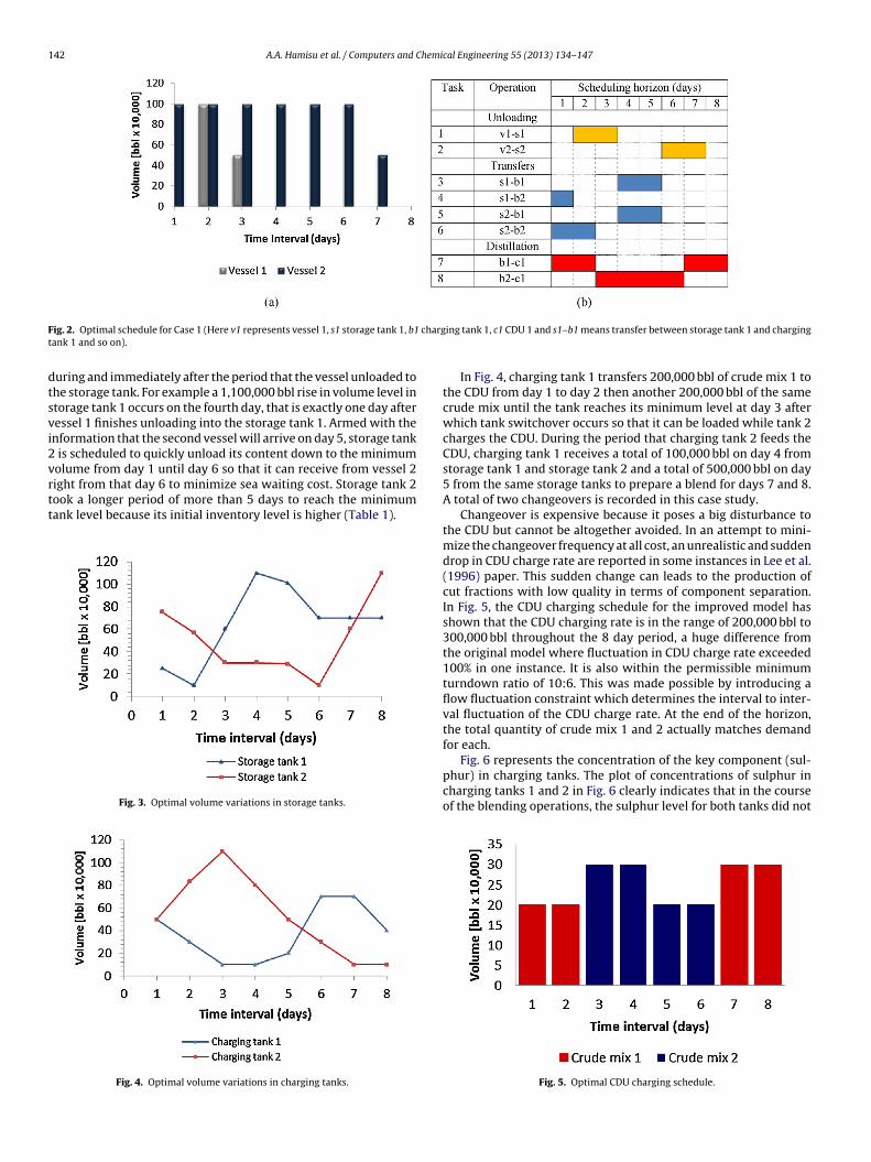
142 A.A. Hamisu et al. / Computers and Chemical Engineering 55 (2013) 134– 147

F chargt

dtsvi2vrtt

ig. 2. Optimal schedule for Case 1 (Here v1 represents vessel 1, s1 storage tank 1, b1ank 1 and so on).

uring and immediately after the period that the vessel unloaded tohe storage tank. For example a 1,100,000 bbl rise in volume level intorage tank 1 occurs on the fourth day, that is exactly one day afteressel 1 finishes unloading into the storage tank 1. Armed with thenformation that the second vessel will arrive on day 5, storage tank

is scheduled to quickly unload its content down to the minimumolume from day 1 until day 6 so that it can receive from vessel 2

ight from that day 6 to minimize sea waiting cost. Storage tank 2ook a longer period of more than 5 days to reach the minimumank level because its initial inventory level is higher (Table 1).

Fig. 3. Optimal volume variations in storage tanks.

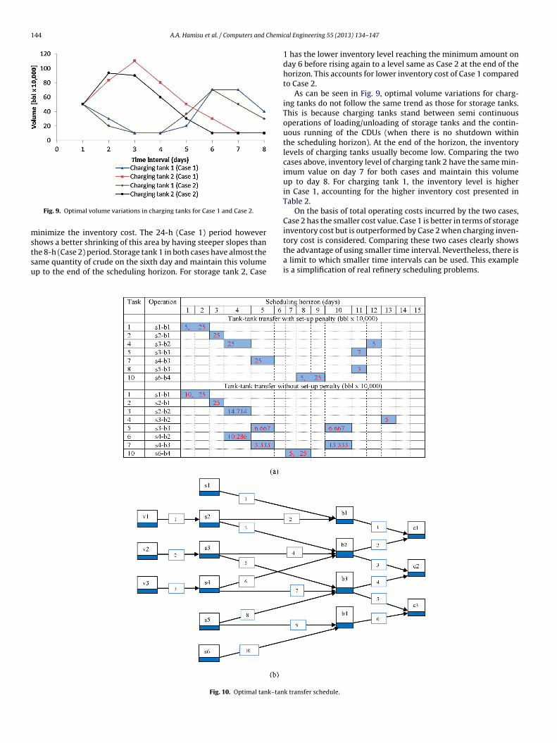
Fig. 4. Optimal volume variations in charging tanks.

ing tank 1, c1 CDU 1 and s1–b1 means transfer between storage tank 1 and charging

In Fig. 4, charging tank 1 transfers 200,000 bbl of crude mix 1 tothe CDU from day 1 to day 2 then another 200,000 bbl of the samecrude mix until the tank reaches its minimum level at day 3 afterwhich tank switchover occurs so that it can be loaded while tank 2charges the CDU. During the period that charging tank 2 feeds theCDU, charging tank 1 receives a total of 100,000 bbl on day 4 fromstorage tank 1 and storage tank 2 and a total of 500,000 bbl on day5 from the same storage tanks to prepare a blend for days 7 and 8.A total of two changeovers is recorded in this case study.

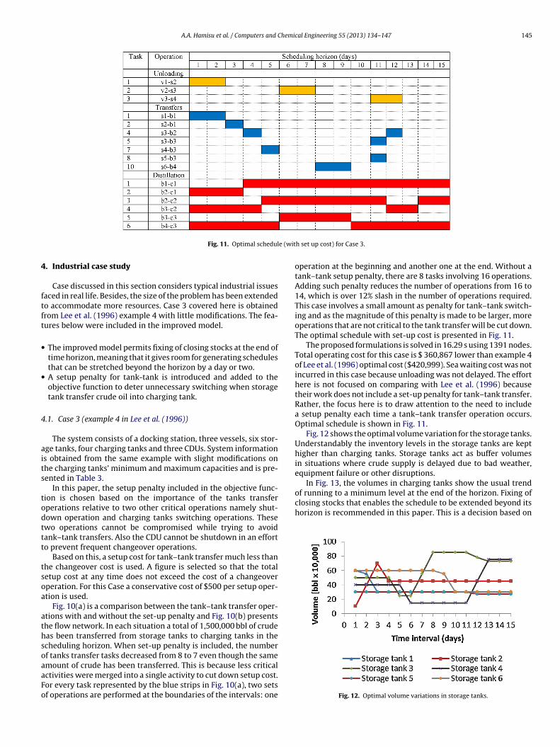
Changeover is expensive because it poses a big disturbance tothe CDU but cannot be altogether avoided. In an attempt to mini-mize the changeover frequency at all cost, an unrealistic and suddendrop in CDU charge rate are reported in some instances in Lee et al.(1996) paper. This sudden change can leads to the production ofcut fractions with low quality in terms of component separation.In Fig. 5, the CDU charging schedule for the improved model hasshown that the CDU charging rate is in the range of 200,000 bbl to300,000 bbl throughout the 8 day period, a huge difference fromthe original model where fluctuation in CDU charge rate exceeded100% in one instance. It is also within the permissible minimumturndown ratio of 10:6. This was made possible by introducing aflow fluctuation constraint which determines the interval to inter-val fluctuation of the CDU charge rate. At the end of the horizon,the total quantity of crude mix 1 and 2 actually matches demandfor each.

Fig. 6 represents the concentration of the key component (sul-phur) in charging tanks. The plot of concentrations of sulphur incharging tanks 1 and 2 in Fig. 6 clearly indicates that in the courseof the blending operations, the sulphur level for both tanks did not

Fig. 5. Optimal CDU charging schedule.

A.A. Hamisu et al. / Computers and Chemical Engineering 55 (2013) 134– 147 143

epiac2ecc

3

sacncio

d2twd

Table 2Comparison between optimal cost for Cases 1 and 2.

Cost Case 1 (24-h period) Case 2 (8-h period)

Sea waiting cost ($) 10,000 0Unloading cost ($) 48,000 40,050Storage tank inventory cost ($) 3358 4630Charging tank inventory cost ($) 5067 4780Changeover cost ($) 150,000 150,000Operating cost ($) 216,425 199,460

Fig. 6. Optimal variation in concentration of sulphur.

xceed their maximum levels specified. Ideally, the variation of sul-hur concentration in tanks should be constant on days when there

s no transfer of crude into the tanks. However, a minor discrep-ncy is noted here, for example, in charging tank 1, the sulphuroncentrations are 0.020 vol/vol and 0.017 vol/vol on days 1 and

respectively. This discrepancy is due to the linearized bilinearquation used to avoid non-linearity in the model. Despite this dis-repancy, the maximum level of sulphur was not exceeded in theharging tanks.

.2. Case 2 (motivating example in Lee et al. (1996))

This case is same as Case 1 except that the horizon is furtherplitted into 8-h time interval. An 8-h time period is chosen because

typical refinery operates based on 8-h shift. The total operatingost of $199,460 was obtained after 17,630 iterations using 247odes in 2.380 s. The 8-h schedule results in a difference of $16,965ompared to the 24-h schedule (Case 1). Table 2 shows a compar-son between the various costs incurred for Cases 1 and 2 and theptimal schedule for both cases is presented in Fig. 7.

The vessel unloading schedule for the two cases shows a slightifference as vessel 1 and vessel 2 starts unloading earlier in Case

. It is obvious from Fig. 7 that the two vessels starts unloading onhe actual days determined at the planning level incurring no seaaiting costs. Vessel 1 has to stop unloading after 8hr of the firstay in order for storage tank 1 to transfer crude to charging tank

Fig. 7. Comparison of optimal s

Fig. 8. Optimal volume variations in storage tanks for Case 1 and Case 2.

2. This decision would be hidden if 24hr time period is adopted asit basically reveal information from day to day without exploringother events happening within the day. For discrete-time represen-tation, using smaller time intervals creates more decision points,giving the model more flexibility in searching for optimal valuesfor the decision variables. For example the first changeover opera-tion in Case 1 could be assumed to have taken place at the end ofthe second day which is not true. The second changeover operationis equally delayed to the end of sixth day implying that the CDUmay not have a sufficient amount of crude to sustain it on the sev-enth day. The two cases recorded the same number of changeoveroperations. The inventory levels are also compared and presentedin Figs. 8 and 9.

Since storage inventory cost depends on both the quantity andtime of storage, it is a direct function of the area bounded by thecurve and the two axes. In Fig. 8, volume variation for both the24-h and 8-h curves have shown a shrinking of these areas to

chedule for Cases 1 and 2.

144 A.A. Hamisu et al. / Computers and Chemi

mstsu

tory cost is considered. Comparing these two cases clearly shows

Fig. 9. Optimal volume variations in charging tanks for Case 1 and Case 2.

inimize the inventory cost. The 24-h (Case 1) period however

hows a better shrinking of this area by having steeper slopes thanhe 8-h (Case 2) period. Storage tank 1 in both cases have almost theame quantity of crude on the sixth day and maintain this volumep to the end of the scheduling horizon. For storage tank 2, Case

Fig. 10. Optimal tank–tan

cal Engineering 55 (2013) 134– 147

1 has the lower inventory level reaching the minimum amount onday 6 before rising again to a level same as Case 2 at the end of thehorizon. This accounts for lower inventory cost of Case 1 comparedto Case 2.

As can be seen in Fig. 9, optimal volume variations for charg-ing tanks do not follow the same trend as those for storage tanks.This is because charging tanks stand between semi continuousoperations of loading/unloading of storage tanks and the contin-uous running of the CDUs (when there is no shutdown withinthe scheduling horizon). At the end of the horizon, the inventorylevels of charging tanks usually become low. Comparing the twocases above, inventory level of charging tank 2 have the same min-imum value on day 7 for both cases and maintain this volumeup to day 8. For charging tank 1, the inventory level is higherin Case 1, accounting for the higher inventory cost presented inTable 2.

On the basis of total operating costs incurred by the two cases,Case 2 has the smaller cost value. Case 1 is better in terms of storageinventory cost but is outperformed by Case 2 when charging inven-

the advantage of using smaller time interval. Nevertheless, there isa limit to which smaller time intervals can be used. This exampleis a simplification of real refinery scheduling problems.

k transfer schedule.

A.A. Hamisu et al. / Computers and Chemical Engineering 55 (2013) 134– 147 145

e (wit

4

ftft

•

•

4

aits

todttt

tsoa

athsoaaFo

of running to a minimum level at the end of the horizon. Fixing ofclosing stocks that enables the schedule to be extended beyond itshorizon is recommended in this paper. This is a decision based on

Fig. 11. Optimal schedul

. Industrial case study

Case discussed in this section considers typical industrial issuesaced in real life. Besides, the size of the problem has been extendedo accommodate more resources. Case 3 covered here is obtainedrom Lee et al. (1996) example 4 with little modifications. The fea-ures below were included in the improved model.

The improved model permits fixing of closing stocks at the end oftime horizon, meaning that it gives room for generating schedulesthat can be stretched beyond the horizon by a day or two.A setup penalty for tank-tank is introduced and added to theobjective function to deter unnecessary switching when storagetank transfer crude oil into charging tank.

.1. Case 3 (example 4 in Lee et al. (1996))

The system consists of a docking station, three vessels, six stor-ge tanks, four charging tanks and three CDUs. System informations obtained from the same example with slight modifications onhe charging tanks’ minimum and maximum capacities and is pre-ented in Table 3.

In this paper, the setup penalty included in the objective func-ion is chosen based on the importance of the tanks transferperations relative to two other critical operations namely shut-own operation and charging tanks switching operations. Thesewo operations cannot be compromised while trying to avoidank–tank transfers. Also the CDU cannot be shutdown in an efforto prevent frequent changeover operations.

Based on this, a setup cost for tank–tank transfer much less thanhe changeover cost is used. A figure is selected so that the totaletup cost at any time does not exceed the cost of a changeoverperation. For this Case a conservative cost of $500 per setup oper-tion is used.

Fig. 10(a) is a comparison between the tank–tank transfer oper-tions with and without the set-up penalty and Fig. 10(b) presentshe flow network. In each situation a total of 1,500,000 bbl of crudeas been transferred from storage tanks to charging tanks in thecheduling horizon. When set-up penalty is included, the numberf tanks transfer tasks decreased from 8 to 7 even though the same

mount of crude has been transferred. This is because less criticalctivities were merged into a single activity to cut down setup cost.or every task represented by the blue strips in Fig. 10(a), two setsf operations are performed at the boundaries of the intervals: one

h set up cost) for Case 3.

operation at the beginning and another one at the end. Without atank–tank setup penalty, there are 8 tasks involving 16 operations.Adding such penalty reduces the number of operations from 16 to14, which is over 12% slash in the number of operations required.This case involves a small amount as penalty for tank–tank switch-ing and as the magnitude of this penalty is made to be larger, moreoperations that are not critical to the tank transfer will be cut down.The optimal schedule with set-up cost is presented in Fig. 11.

The proposed formulations is solved in 16.29 s using 1391 nodes.Total operating cost for this case is $ 360,867 lower than example 4of Lee et al. (1996) optimal cost ($420,999). Sea waiting cost was notincurred in this case because unloading was not delayed. The efforthere is not focused on comparing with Lee et al. (1996) becausetheir work does not include a set-up penalty for tank–tank transfer.Rather, the focus here is to draw attention to the need to includea setup penalty each time a tank–tank transfer operation occurs.Optimal schedule is shown in Fig. 11.

Fig. 12 shows the optimal volume variation for the storage tanks.Understandably the inventory levels in the storage tanks are kepthigher than charging tanks. Storage tanks act as buffer volumesin situations where crude supply is delayed due to bad weather,equipment failure or other disruptions.

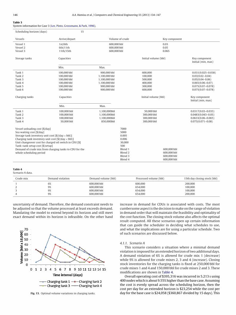
In Fig. 13, the volumes in charging tanks show the usual trend

Fig. 12. Optimal volume variations in storage tanks.

146 A.A. Hamisu et al. / Computers and Chemical Engineering 55 (2013) 134– 147

Table 3System information for Case 3 (Lee, Pinto, Grossmann, & Park, 1996).

Scheduling horizon (days) 15

Vessels Arrive/depart Volume of crude Key component

Vessel 1 1st/6th 600,000 bbl 0.03Vessel 2 6th/11th 600,000 bbl 0.05Vessel 3 11th/15th 600,000 bbl 0.065

Storage tanks Capacities Initial volume (bbl) Key componentInitial (min, max)

Min. Max.

Tank 1 100,000 bbl 900,000 bbl 600,000 0.031(0.025–0.038)Tank 2 100,000 bbl 1,100,000 bbl 100,000 0.03(0.02–0.04)Tank 3 100,000 bbl 1,100,000 bbl 500,000 0.05(0.04–0.06)Tank 4 100,000 bbl 1,100,000 bbl 400,000 0.065(0.06–0.07)Tank 5 100,000 bbl 900,000 bbl 300,000 0.075(0.07–0.078)Tank 6 100,000 bbl 900,000 bbl 600,000 0.075(0.07–0.078)

Charging tanks Capacities Initial volume (bbl) Key componentInitial (min, max)

Min. Max.

Tank 1 100,000 bbl 1,100,000bbl 50,000 bbl 0.0317(0.03–0.035)Tank 2 100,000 bbl 1,100,000bbl 300,000 bbl 0.0483(0.043–0.05)Tank 3 100,000 bbl 1,100,000bbl 300,000 bbl 0.0633(0.06–0.065)Tank 4 50,000 bbl 850,000bbl 300,000 bbl 0.075(0.071–0.08)

Vessel unloading cost [$/day] 7000Sea waiting cost [$/day] 5000Storage tank inventory unit cost [$/(day × bbl)] 0.005Charging tank inventory unit cost [$/(day × bbl)] 0.006Unit changeover cost for charged oil switch in CDU [$] 30,000Tank–tank setup cost [$/setup] 500Demand of crude mix from charging tanks to CDU for thewhole scheduling period

Blend 1 600,000 bblBlend 2 600,000 bblBlend 3 600,000 bblBlend 4 600,000 bbl

Table 4Scenario A data.

Crude mix Demand violation Demand volume (bbl) Processed volume (bbl) 15th day closing stock (bbl)

1 6% 600,000 bbl 600,000 200,000

ubMe

2 9% 600,000 bbl

3 9% 600,000 bbl

4 9% 600,000 bbl

ncertainty of demand. Therefore, the demand constraint needs to

e adjusted so that the volume processed at least exceeds demand.andating the model to extend beyond its horizon and still meet

xact demand within its horizon is infeasible. On the other hand

Fig. 13. Optimal volume variations in charging tanks.

654,000 100,000654,000 100,000654,000 200,000

increase in demand for CDUs is associated with costs. The mostcumbersome aspect is the decision to make on the range of violationin demand order that will maintain the feasibility and optimality ofthe cost function. The closing stock volume also affects the optimalresult computed. All these scenarios open up certain informationthat can guide the scheduler in deciding what schedules to use,and what the implications are for using a particular schedule. Twoof such scenarios are discussed below.

4.1.1. Scenario AThis scenario considers a situation where a minimal demand

violation is imposed for an extended horizon of two additional days.A demand violation of 6% is allowed for crude mix 1 (decrease)while 9% is allowed for crude mixes 2, 3 and 4 (increase). Closingstock inventories for the charging tanks is fixed at 250,000 bbl forcrude mixes 1 and 4 and 150,000 bbl for crude mixes 2 and 3. Thesemodifications are shown in Table 4.

Overall operating cost of $395,316 was incurred in 5.213 s using

400 nodes which is about 9.55% higher than the base case. Assumingthe cost is evenly spread across the scheduling horizon, then thecost per day for an extended horizon is $23,254 while the cost perday for the base case is $24,058 ($360,867 divided by 15 days). This

A.A. Hamisu et al. / Computers and Chemi

Table 5Scenario B data.

Crude mix Demand volume(bbl)

Processed volume(bbl)

15th day closingstock (bbl)

1 600,000 620,000 300,000

ib

eTwitoc2

4

tsif

netI$2bsp

5

ip(iwadtssmhcto

(wo

2 600,000 654,000 200,0003 600,000 650,000 150,0004 600,000 654,000 250,000

s about 3.34% cut in daily operating cost when compared to thease case.

Because of the demand violation, quantity of crude mix 1 meetsxact demand, while crude mixes 2, 3 and 4 were above demand.he quantity of crude mix 1 processesed meets exact demand evenhen violation of 6% is allowed; this is because the improved model

s more sensitive to the increase in demand order. Demand viola-ion of 6% up to 88% for crude mix 1 does not change the optimalperating cost. However, with violation above 88% the operatingost assumed a different value. Violation in demand of crude mix, 3 or 4 below 9% generates infeasible solution.

.1.2. Scenario BHere demand violation for all the crude mixes are allowed so

hat all the CDUs process above demand. When the same closingtock for scenario A was used the model was infeasible because ofnsufficient stock in the charging tanks. The 15th day closing stockor these tanks were increased as in Table 5.

The operating cost is $394,500 generated in 28.892 s using 2640odes. It is obvious from the results that scenario B is more costffective as compared with scenario A. This can be verified fur-her by comparing total operating cost with the volume processed.n scenario A, a total of 2,562,000 bbl was processed at a cost of395,316 which is about $0.1543 per barrel. Scenario B handles,578,000 bbl at a cost of $394,500 which is about $0.1530 perarrel. Comparing just the operating costs for the two scenarios,cenario B involves a smaller operating cost. Also, when the coster barrel is compared, scenario B is still a better option to go by.

. Conclusions

In this paper, an existing MILP model of Lee et al. (1996)s improved to make it reflect real life scheduling problem inetroleum refinery plant. Three cases from examples in Lee et al.1996) were used to test the improved model. The model ismproved by adding interval–interval volume variation constraint

hich prevents widely fluctuating CDU charging rate and included CDU shutdown penalty which consider the possibility of shut-own within the scheduling cycle. A setup penalty for tank–tankransfer is included in Case 3. Some level of flexibility is introducedo that demand violation is permitted when exact demand con-traints lead to infeasibility in scenario A of Case 3. The improvedodel permits fixing of closing stocks at the end of scheduling

orizon to explore the impact of increase/decrease in CDUs mixrude oil demand from charging tanks. Overall, the improved modelranslates into a decrease in operating cost and offers more flexibleperation.

Data for Case 1 and Case 2 were obtained from Yüzgec et al.2010) and from Lee et al. (1996) for Case 3. The improved modelas implemented using CPLEX solver in GAMS and the results

btained have shown that the model adequately represents the

cal Engineering 55 (2013) 134– 147 147

problem statement. Two scenarios were created from the indus-try size problem (Case 3) to offer the scheduler with options thatwill aid decision on the best schedule to use.

Acknowledgement

The first two authors would like to acknowledge the finan-cial support from Petroleum Technology Development Fund (PTDF)Nigeria under the fund’s overseas scholarship scheme.

References

Bassett, M. H., Pekny, J. F., & Reklaitis, G. V. (1996). Decomposition techniques forthe solution of large-scale scheduling problems. AIChE Journal, 42, 3373.

Harjunkoski, I., & Grossmann, I. E. (2001). A decomposition approach for thescheduling of a steel plant production. Computers and Chemical Engineering, 25,1647–1660.

Jia, Z., Ierapetritou, M., & Kelly, J. D. (2003). Refinery short-term scheduling usingcontinuous-time formulation: Crude oil operations. Industrial and EngineeringChemistry Research, 42, 3085–3097.

Karri, B., Srinivasan, R., & Karimi, I. A. (2009). Robustness measures for operationschedules subject to disruptions. Industrial and Engineering Chemistry Research,48, 9204–9214.

Kelly, J. D., & Mann, J. L. (2003). Crude oil blend scheduling optimization: An applica-tion with multi-million dollar benefits-part 2. Hydrocarbon Processing, 82, 72–79.

Kondili, E., Pantelides, C. C., & Sargent, R. W. H. (1993). A general algorithm forshort-term scheduling of batch operations – I. MILP formulation. Computers andChemical Engineering, 17, 211–227.

Lee, H., Pinto, J. M., Grossmann, I. E., & Park, S. (1996). Mixed-integer linear pro-gramming model for refinery short-term scheduling of crude oil unloadingwith inventory management. Industrial and Engineering Chemistry Research, 35,1630–1641.

Li, J., Li, W., Karimi, I. A., & Srinivasan, R. (2007). Improving the robustness andefficiency of crude scheduling algorithms. AIChE Journal, 53(10), 2659–2680.

Li, W., Hui, C. W., Hua, B., & Tong, Z. (2002). Scheduling crude oil unload-ing, storage, and processing. Industrial and Engineering Chemistry Research, 41,6723–6734.

Moro, L. F. L., & Pinto, J. M. (2004). Mixed-integer programming approach for short-term crude oil scheduling. Industrial and Engineering Chemistry Research, 43,85–94.

Mouret, S., Grossmann, I. E., & Pestiaux, P. (2009). A novel priority-slot basedcontinuous-time formulation for crude-oil scheduling problems. Industrial andEngineering Chemistry Research, 48, 8515–8528.

Pan, M., Li, X., & Qian, Y. (2009). New approach for scheduling crude oil operations.Chemical Engineering Science, 64, 965–983.

Pinto, J. M., Joly, M., & Moro, L. F. L. (2000). Planning and scheduling models forrefinery operations. Computers and Chemical Engineering, 24, 2259–2276.

Reddy, P. C. P., Karimi, I. A., & Srinivasan, R. (2003). Short-term scheduling of refineryoperations from unloading crudes to distillation, process system engineering.Computer Aided Chemical Engineering, 15, 304–309.

Saharidis, G. K. D., & Ierapetritou, M. G. (2009). Scheduling of loading and unload-ing of crude oil in a refinery with optimal mixture preparation. Industrial andEngineering Chemistry Research, 48, 2624–2633.

Saharidis, G. K. D., Minoux, M., & Dallery, Y. (2009). Scheduling of loading andunloading of crude oil in a refinery using event-based discrete time formulation.Computers and Chemical Engineering, 33, 1413–1426.

Shah, N., Saharidis, K. D. G., Jia, Z., & Ierapetritou, M. G. (2009). Centralized-decentralized optimization for refinery scheduling. Computers and ChemicalEngineering, 33, 2091–2105.

Shah, N. K., Li, Z., & Ierapetritou, G. M. (1996). Petroleum refining operations:Key issues, advances and opportunities. Industrial and Engineering ChemistryResearch, 50, 1161–1170.

Westerlund, J., Hastbacka, M., Forssell, S., & Westerlund, T. (2007). Mixed-timemixed-integer linear programming scheduling model. Industrial and EngineeringChemistry Research, 46, 2781–2796.

Wu, N., Chu, C., Chu, F., & Zhou, M. (2011). Schedulability analysis of short-termscheduling for crude oil operations in refinery with oil residency time andcharging-tank-switch-overlap constraints. IEEE Transanctions of Automation Sci-ence and Engineering, 8(1), 190–204.

Yee, K. L., & Shah, N. (1998). Improving the efficiency of discrete-time schedulingformulation. Computers and Chemical Engineering, 22, S403–S410.

Yüzgec , U., Palazoglu, A., & Romagnoli, J. A. (2010). Refinery scheduling of crudeoil unloading, storage and processing using a model predictive control strategy.Computers and Chemical Engineering, 34, 1671–1686.