Forecasting Implied Volatility Smile Surface via Deep ... - arXiv

1 Shengli Chen [email protected] Harvest Fund & Peking University

Forecasting Implied Volatility Smile Surface via Deep Learning and Attention Mechanism①

Shengli Chen1,2, Zili Zhang 2

1. Guanghua School of Management, Peking University, Beijing 100871

2. Harvest Fund Management Co., Ltd., Beijing 100005

Abstract: The implied volatility smile surface is the basis of option pricing, and the dynamic evolution of the

option volatility smile surface is difficult to predict. In this paper, attention mechanism is introduced into LSTM,

and a volatility surface prediction method combining deep learning and attention mechanism is pioneeringly

established. LSTM's forgetting gate makes it have strong generalization ability, and its feedback structure enables it

to characterize the long memory of financial volatility. The application of attention mechanism in LSTM networks

can significantly enhance the ability of LSTM networks to select input features. This paper considers the discrete

points of the implied volatility smile surface as an overall prediction target, extracts the daily, weekly, and monthly

option implied volatility as input features and establishes a set of LSTM-Attention deep learning systems. Using

the dropout mechanism in training reduces the risk of overfitting. For the prediction results, we use arbitrage-free

smoothing to form the final implied volatility smile surface. This article uses the S&P 500 option market to conduct

an empirical study. The research shows that the error curve of the LSTM-attention prediction system converges,

and the prediction of the implied volatility surface is more accurate than other predicting system. According to the

implied volatility surface of the 3-year rolling forecast, the BS formula is used to pricing the option contract, and

then a time spread strategy and a butterfly spread strategy are constructed respectively. The experimental results

show that the two strategies constructed using the predicted implied volatility surfaces have higher returns and

Sharpe ratios than that the volatility surfaces are not predicted. This paper confirms that the use of AI to predict

the implied volatility surface has theoretical and economic value. The research method provides a new reference

for option pricing and strategy.

Keywords: LSTM, attention mechanism, deep learning, volatility smile surface, spread strategy.

1 Introduction

Volatility is one of the key attributes of asset prices and a key variable in the pricing of options contracts. In

the classic Black-Scholes-Merton (BSM) option pricing model, it is assumed that the volatility is constant, and the

implied volatility is the asset price, exercise price, remaining period, risk-free interest rate, bonus interest rate, etc.

Given those parameters, the market price of the European option is substituted into the BSM pricing formula to

reverse the volatility. According to the assumption of the BSM option pricing formula, the implied volatility is a

Biography:

Shengli Chen, Ph.D. in Management, He is Postdoctoral Research Fellow at the Peking University - Harvest Fund joint

postdoctoral research station. His research interests Artificial Intelligence and Quantitative Investment. His

representative paper titled “Forecasting Realized volatility of Chinese Stock Index Futures based on Jumps, Good-bad

Volatility and Baidu Index” was published in the Systems Engineering — Theory & Practice（Issue 2, 2018) (in Chinese).

E-mail: [email protected].

Zili Zhang, Ph.D. in Theoretical Physics, University of Texas at Austin, Managing Director of Harvest Fund Management

Co., Ltd., Head of AI Investment & Research Center, Fund Manager. His research focuses on Artificial Intelligence and

Quantitative Investments. His representative paper titled “Stock Network, Systematic Risk and Stock Pricing Implications”

will be published in the Quarterly Journal of Economics (forthcoming in 2020.1) (in Chinese). E-mail: [email protected]

Fund: The paper is funded by the First-class Project of China Postdoctoral Science Foundation (2018M640367)

Working paper, 2019-12-23


constant that has nothing to do with the exercise price and the remaining period of the option. However, what

people observe in the market is that the implied volatility varies with the exercise price and the remaining term.

By plotting the implied volatility corresponding to options with different durations and different exercise prices in

a three-dimensional space composed of terms, exercise prices, and implied volatility, a so-called "implicit volatility

surface" is formed. Moreover, a large number of studies have also found that the shape of the implied volatility

surface is not static, but shows obvious time-varying characteristics over time (Dumas et al., 1998; Cont et al.,

2002; Fengler et al., 2007). Today, scholars generally accept the view that the implied volatility surface at a given

point in time appears as a surface shape related to the strike price and the expiration date, and is dynamically

changing in the time dimension (Goncalves et al., 2006).

Volatility is one of the key attributes of asset prices and a key variable in the pricing of options contracts. In

the classic Black-Scholes-Merton (BSM) option pricing model, it is assumed that the volatility is constant, and the

implied volatility is the asset price, strike price, and balance given the implicit volatility surface. The question to be

studied in this article is: Can the dynamic change of the implied volatility surface be predicted, and how to predict

it? The predictability of asset prices is an eternal theme of financial research, and the predictability of option

prices is no exception. However, due to the complexity of options, it is difficult to directly study the predictability

of option prices. When the parameters of the BSM option pricing model are known, the corresponding implied

volatility can be calculated by giving the fixed-term price, and the implied volatility can be reversed to the option

price. Therefore, the option price and the implied volatility are formed. The one-to-one correspondence naturally

becomes a surrogate variable for studying the nature of option prices. If you can accurately predict the changes in

implied volatility, you can effectively predict the changes in option prices, which is of great significance to options

trading and risk management. In addition, the implied volatility itself contains market participants' expectations of

the future volatility of the underlying asset. Research on the predictability of the implied volatility can further

identify the market risk of the underlying asset. Therefore, the dynamic modeling and extrapolation of the implied

volatility surface have a fundamental effect on both the option itself and the underlying asset.

In the field of implicit volatility surface prediction, there are not many research results. There are two main

reasons. First, high-dimensional research is too difficult. It is obviously more difficult to study the dynamic process

of the volatility surface than the dynamic process of the stock price (single point) and the dynamic process of the

term structure of interest rates (a line); Confused with the prediction of "implied volatility." Historical volatility is

the volatility calculated based on the underlying asset price series, such as standard deviation, idiosyncratic

volatility, and realized volatility. In recent years, many scholars have established a series of methods such as

GARCH models and HAR models to predict the realized volatility. The implied volatility of the options to be

predicted in this article is a direct reflection of the future volatility expectations formed by the market in options

trading, which is completely different from the connotation of historical volatility, which will necessarily make its

properties, characteristics and research methods different. . Compared with the prediction research of historical

volatility, there are few researches on the prediction of implied volatility.

In the research literature of implicit volatility surface prediction, Carr et al. (2016) used the arbitrage-free

condition to derive the expression of the implicit volatility surface, describing the dynamic behavior of the implicit

volatility surface, but these studies did not involve the prediction of implied volatility. Guidolin et al. (2003) and

Garcia et al. (2003) theoretically analyzed the possibility of predicting implied volatility using mechanism

transformation and information learning models. Harvey et al. (1992), Guo (2000), Brooks et al. (2002)

respectively studied the predictability of the implied volatility of S&P100 stock index options, foreign exchange

options, and government bond options, but these studies only focused on the implied volatility of short-term

options rather than the entire volatility surface. In addition, Fernandes et al. (2014), Konstantinidi et al. (2008)

used the volatility index VIX to study the predictability of implied volatility, which is also not for the entire volatility


surface. Researches similar to this article are Dumas et al. (1998), Goncalves et al. (2006), Bernales et al. (2014).

Dumas et al. (2014) first used a two-step method to construct an implicit volatility surface. In the first step, the

implied volatility surface is expressed as a function of the moneyness and the remaining period; in the second step,

a time series model is constructed for the coefficients of cross-sectional regression. Goncalves et al. (2006) also

used a two-step method to construct a dynamic model of the implied volatility surface of the S&P500 index option,

and then tested the predictability of the implied volatility from a statistical significance. Based on the two-step

method to establish the implied volatility surface model, Bernales et al. (2014) studied the predictability of the

implied volatility surface of US stock options, and obtained similar conclusions as the above study.

Advances in artificial intelligence technology have provided new methods for financial engineering research.

Hochreiter (1997) first proposed long short-term memory (LSTM). With the rise of deep learning, LSTM has a large

number of applications in engineering fields such as natural language processing and language recognition. The

LSTM has been cited in the prediction of financial time series for several reasons: 1) The feedback structure of the

LSTM enables it to characterize the long memory effect of financial time series, especially for the volatility of

financial assets; 2) LSTM has a unique forgetting gate, which reduces the risk of over-fitting the neural network

and makes it have stronger out-of-sample prediction capabilities; 3) LSTM is an open prediction framework that

can adapt Adjusting the weight of the input features on the ground has a stronger mode approximation ability

than traditional linear models. In addition, in the field of machine translation, the Google team proposed an

attention model that simulates the human brain (Ashish et al, 2017). The attention mechanism is mainly used to

simulate the human perspective system, and jumps to different objects and positions in the entire field of view, so

as to perform analysis and processing resource allocation and coordination. When human eyes look at a painting,

they often focus on a small piece. At this time, the corresponding weight of the Attention model becomes larger.

Introducing the attention mechanism into the LSTM structure can significantly enhance the automatic screening

and optimization capabilities of LSTM input features. At present, there is no financial literature that uses LSTM and

attention models for the modeling and forecasting of implicit volatility surfaces. This article will turn on artificial

intelligence research methods are of great significance for modeling and forecasting of implicit volatility surfaces

of options.

The structure of this paper is as follows: Section 1 is the introduction of the paper; Section 2 describes the

theoretical research methods of this paper, including option pricing and implicit volatility theory, and the

attention-based LSTM deep learning prediction system; Section 3 expands on Empirical research, including data

sources, data, prediction results of deep learning models, and analysis of options spread strategies. Section 4

summarizes and looks forward.

2. Theoretical methods

2.1 Option pricing and implied volatility

This section first describes the landmark BS option pricing formula. In the field of option pricing research,

scholars Black, Scholes, and Merton pioneered the BS model (or the BSM model) and were awarded the Nobel

Prize in Economics. Under many necessary assumptions, Black, Scholes, and Merton established the following

famous B-S-M differential equations:

2

2 2

2

1

2

f f frS s rf

t s s

(1)

Through the derivation of the above differential equation, we finally get the BS pricing formula for call and put

options:


0 1 2N( ) N( )rTC S d Ke d (2)

2 0 1N( ) N( )rTP Ke d S d (3)

2

0

1

ln 2=

S K r Td

T

(4)

2

0

2

ln + 2=

S K r Td

T

(5)

In the above formula, C represents the price of call options; P represents the price of put options; 0S is the

starting price of the underlying asset; r is the risk-free interest rate of continuous compounding; is the

volatility of the underlying asset; T is the term of the option; N( ) is the cumulative probability distribution

function of the standard normal distribution; 1d describes the sensitivity of the option to the underlying price,

and 2d describes the possibility of the option being finally executed. Therefore, the theoretical prices of call and

put options can be expressed by the BS formula as expressions of starting price, exercise price, risk-free interest

rate, asset volatility and option duration.

Implied volatility is a core variable in option pricing and investment trading. Implied volatility refers to the

implied volatility of the market price of an option. The most common method for estimating implied volatility is to

substitute the market price of options into the BS formula and calculate implied volatility backwards. In other

words, according to the BS formula, we can calculate the implied volatility at a certain moment at a specific strike

price. As the option exercise price changes, the implied volatility calculated by the BS formula presents a smile

curve, that is, the volatility smile curve, which describes the relationship between the implied volatility of the

option and the exercise price function. On this basis, if the change of the term is further considered, the implied

volatility calculated by the BS formula will form a three-dimensional volatility smile surface. In actual options

trading, investors often use the volatility smile curve and volatility smile surface to analyze and find trading

opportunities.

Because the exercise price and term of the option contract are discrete, the implied volatility smile surface

calculated by using the BS formula to calculate backwards point by point is also discretized and presents an

uneven surface. On this basis, academia and practice circles usually perform non-arbitrage smoothing, and finally

get a smoother volatility smile surface. The real significance of the predicted volatility smile surface is that the

next period of option contracts can be priced based on the predicted volatility surface, thereby laying the

foundation for the study of option strategies.

2.2 Recurrent neural networks

Recurrent neural networks (RNNs, also known as "feedback neural networks") are an extension of

feed-forward neural networks, which include feedback hidden layers (recurrent hidden states), whose output in

the current state depends on the value of the previous state. Given the input vector of the neural network:

1 2( , , , , , )t nx x x x x (6)

The recurrent neural network updates its feedback hidden layer vector by the formula:

1( )t t t h Wx Uh b (7)


where the note b represents the deviation vector and represents the activation function of the feedback

hidden layer. The expanded structure of a recurrent neural network is shown in Figure 1. The figure shows that the

recurrent neural network in the feedback hidden layer ( )A t at state t contains the input vector tx and the

feedback hidden layer output vector 1th of the previous state, and calculates a new output vector th . In this

process, the state of ( )A t is passed from the previous step to the next step. Therefore, a recurrent neural

network is theoretically the result of a finite number of replications of the same neural network structure. At

present, recurrent neural networks have been widely used in the research of cutting-edge issues such as speech

recognition, language models, machine translation, and timing analysis, with great success. In the field of financial

market predictive modeling, Danilo and Jonathon et al. (2002) systematically studied the theoretical advantages,

modeling methods, and economic value of RNNs feedback loop structure.

Fig.1 The unfolding structure of recurrent neural network

2.3 Long Short-Term Memory

The working mechanism of recurrent neural networks is to use historical information to assist current

decisions. It can better use information that cannot be modeled by feedforward neural network structures, but it

also brings long-term dependencies to the technology challenge. In many practical prediction problems, useful

information that affects the current state can vary in time from the current state to different lengths. If the time

interval of useful information is short, the training results of RNNs are susceptible to interference by historical

redundant information; if the interval of useful information is long, the loop iteration of RNNs increases a large

number of calculations and it is difficult to capture useful key information. The design of long short-term memory

(LSTM) can effectively solve the above problems faced by RNNs. As a specially designed feedback neural network

structure, LSTM performs better than standard RNNs on many tasks and is one of the most successful

representatives of RNNs engineering practice.

The earliest LSTM was proposed by Hochreiter et al. (1997), which replaced the RNN hidden layer with a

memory block and used a memory cell to store information. In order to enhance the processing capability of LSTM,

Gers et al. (2000) introduced forget gate. Gers et al. (2000, 2002) further proposed peephole connections on this

basis, which added the cell states of the previous state as inputs for three gate structures. Therefore, the current

popular LSTM network structure is shown in Figure 2. The core of the LSTM network structure is three special gate

structures: input gate, output gate, and forget gate.

They are composed of weighted multipliers and sigmoid activation functions. They can predict the output at a

certain moment by remembering or forgetting the accumulated information in the range [0,1]. The forget gate

determines which part of the information needs to be forgotten according to the input tx of the current state,

1tc of the previous state, and output 1th of the previous state. The input gate decides which part of the

information enters the state tc at the current moment according to tx 、

1tc and 1th . Therefore, the gate


structure of LSTM can more effectively decide which information is forgotten and which information should be

retained.

With reference to Gers et al. (2000, 2002) and Alex (2014), the calculation formula of LSTM network is:

1 1( )t ix t ih t ic t i i W x W h W c b (8)

1 1( + )t fx t fh t fc t f f W x W h W c b (9)

1 1( + )t ox t oh t oc t o o W x W h W c b (10)

1( )t gx t gh t g g W x W h b (11)

1t t t t t c f c i g (12)

( )t t th o c (13)

Where , are activation functions, respectively representing sigmoid function and tanh function; is

element-wise multiplication; W is weight matrix; b is error vector; ti 、 tf and to represent input gate, forget

gate, and output gate at time t; tc represents an iterative method of cell states; th represents the network

output. As can be seen in Figure 2, the input gate, forget gate, and output gate are all connected to the point

multiplication node, which respectively represent the states of the input, output, and memory units that control

the LSTM network. The training algorithms for LSTM can be read in Hochreiter et al. (1997) and Gers et al. (2002),

which are not described in this article.

+

+

Input gate

it

gt

+

C

+

Output gate

ot

+

Forget gate

ft

input xt

xt

ht-1

xt

ht-1

xt

ht-1

output ht

ht-1

ct

ct-1

ct-1

ct-1

ct

block input

block output

Fig.2 The structure of long short-term memory network


2.4 Attention mechanism

The Google team first proposed an Attention model that simulates human visual attention mechanism

(Ashish et al, 2017). In recent years, attention models have been widely used in various fields of deep learning.

Whether it is image processing, speech recognition or natural language processing, it is often encountered in

various types of tasks. The visual attention mechanism is a brain signal processing mechanism unique to human

vision. Human vision quickly scans the global image to obtain the target area that needs attention, and then

invests more attention resources in this area to obtain more detailed information about the target that needs

attention, and suppress other useless information. The human visual attention mechanism is a means for humans

to quickly screen out high-value information from a large amount of information using limited attention resources,

which greatly improves the efficiency and accuracy of visual information processing. The attention mechanism in

deep learning is similar to the human visual attention mechanism in essence. The core goal is to select information

that is more critical to the current task goal from a lot of information.

h1 h2 h3 hj hm��

x1 xjx3x2 xm

+

tjα 1tα

2tα 3tα

tmα

stst-1

ct

yt-1 yt

ijα

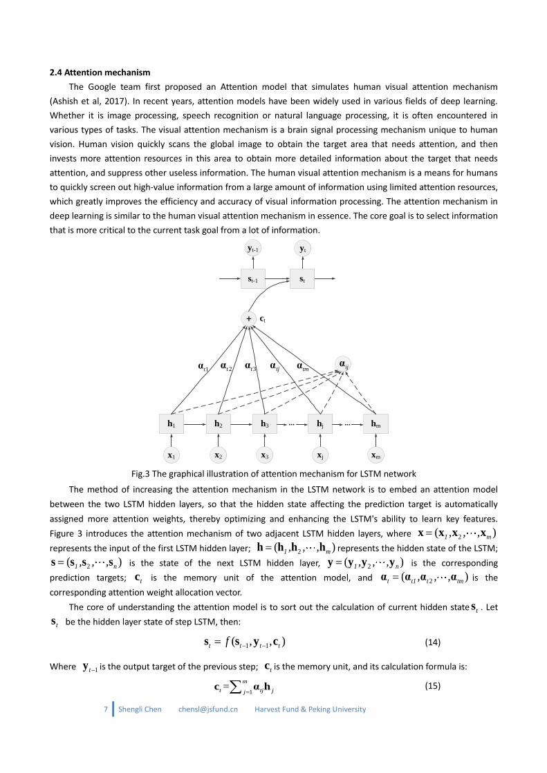
Fig.3 The graphical illustration of attention mechanism for LSTM network

The method of increasing the attention mechanism in the LSTM network is to embed an attention model

between the two LSTM hidden layers, so that the hidden state affecting the prediction target is automatically

assigned more attention weights, thereby optimizing and enhancing the LSTM's ability to learn key features.

Figure 3 introduces the attention mechanism of two adjacent LSTM hidden layers, where 2( )1 m, , ,x x x x

represents the input of the first LSTM hidden layer; 2( )1 m, , ,h h h h represents the hidden state of the LSTM;

2( )1 n, , ,s s s s is the state of the next LSTM hidden layer, 2( )1 n, , ,y y y y is the corresponding

prediction targets; tc is the memory unit of the attention model, and 2( )t t1 t tm, , ,α α α α is the

corresponding attention weight allocation vector.

The core of understanding the attention model is to sort out the calculation of current hidden state ts . Let

ts be the hidden layer state of step LSTM, then:

1 1( , , )t t t tf s s y c (14)

Where 1ty is the output target of the previous step; tc is the memory unit, and its calculation formula is:

1

=m

t tj jjc α h (15)


Where jh is the LSTM hidden layer state corresponding to the input jx of step j ; tjα is the attention distribution

weight of memory unit tjα on hidden layer state jh , and its calculation formula is:

1

exp( )

exp( )

tj

tj m

tkk

e

e

α (16)

where tje is an alignment model, which is a non-linear approximation function 1= ( , )tj t je a s h of the states 1ts

and jh of the two hidden layers before and after the LSTM. To reduce the amount of calculation, this paper uses

a single-layer perceptron as the approximation function:

1 1( , ) tanh( )t j ah j as t aa s h W h W s b (17)

In summary, the attention model takes the hidden layer state 2( )1 m, , ,h h h h of the LSTM as input, and

after calculation and processing of the attention layer (Attention layer), it finally maps to the LSTM hidden layer

state 2( )1 n, , ,s s s s .

2.5 Dropout training mechanism

In deep learning predictive modeling, how to avoid overfitting is a key point in the application of neural

networks. The current effective way is to add a dropout training mechanism to the prediction system. The earliest

dropout training method was first proposed by Hinton et al. (2014), and Yarin (2015) subsequently introduced it to

the training of RNNs. The Dropout training method is mainly used in neural network training to discard part of the

data of the memory unit with a specific probability, thereby reducing the overfitting of the neural network within

the sample and enhancing the generalization ability outside the sample. The Dropout training mechanism can be

used both inside the LSTM memory unit (Yarin, 2015) and outside the LSTM hidden layer. In this paper, the use of

the dropout training mechanism is mainly to modify the state output h of the hidden layer of the LSTM in

network training.

Drawing on Hinton et al. (2014), this article explains the mathematical principles of the dropout training

mechanism. Let {1, , }l L be the number of the hidden layer of the neural network, ( )lh be the output vector

of the l-th hidden layer, ( )lw and

( )lb be the weight vector and the bias vector. As shown in Figure 4 (a), the

calculation formula for the neuron node i is expressed as:

( 1) ( 1) ( ) ( 1)

( 1) ( 1)(z )

l l l l

i i i

l l

i i

z b

y f

w h (18)

Where ( 1)l

iz

is the weighted sum of the input features and f is the activation function. As shown in Figure 4

(b), when the input data of this neuron node uses the dropout training mechanism, its calculation formula is:

( )

( ) ( ) ( )

( 1) ( ) ( 1)

( 1) ( 1)

Bernoulli( )

(z )

l

j

l l l

l l l

i i i

l l

i i

r p

z b

y f

h r h

w h (19)

where ( )lr is a Bernoulli independent and identically distributed vector, and the probability of each element being

1 is p (the probability of 0 is 1-p); ( )lh is the hidden layer output vector after dropout probability correction. It is


worth mentioning that the dropout mechanism is only used for the training of neural networks. In actual

prediction, the neuron node i is calculated according to the non-dropout formula.

( )

1

lh

( )

2

lh

( )l

jh

( )l

mh

1

( 1)l

iz ( 1)l

iy

( 1)l

ib

( 1)l

j

w f

( )

1

lh

( )

2

lh

( )l

jh

( )l

mh

1

( 1)l

iz ( 1)l

iy

( 1)l

ib

( 1)l

j

w f

( )

1

lh

( )

2

lh

( )l

jh

( )l

mh

( )l

mr

�

�

�

�

( )l

jr

( )

1

lr

( )

2

lr

(a) Standard network (b) Dropout network

Fig.4 The basic operations of a standard and dropout network

2.6 Deep Learning Prediction System

The theory of LSTM memory unit, attention model, and dropout training mechanism was explained in the

previous article, but they are only local systems that predict the volatility smile surface. A complete deep learning

prediction system needs to organically combine them. This paper builds an attention-based LSTM deep learning

prediction system for the volatility smile surface prediction, which can be regarded as a deep neural network

model (abbreviated as Att-LSTM) for volatility surface prediction. If the input feature of the prediction system is

Tx , and the prediction target is 1T y , then the mathematical form of the deep learning prediction system

constructed in this paper is 1=Att-LSTM( )T Ty x . The network structure of the Att-LSTM deep learning

prediction system is shown in Figure 5. From bottom to top, the prediction system is input layer, LSTM hidden layer,

dropout training layer, attention layer, LSTM hidden layer, dropout training layer, fully connected layer and output

layer. Therefore, the prediction system includes 2 LSTM hidden layers, 2 dropout training layers, and 1 attention

layer.

The information transfer process of the prediction system includes the following core links. 1) Input layer. For

the prediction target1T y , if the external input of the prediction system is a matrix of dimension T*N, then the

input layer is composed of the feature vectors of adjacent T steps 1 2=( )T Tx ,x , ,xx ,and each step input is a

vector of N input features, that 1 2(x )j j j jN,x , ,xx . 2) The first LSTM hidden layer. Each step of the input

feature jx will correspond to a memory unit in the hidden layer of LSTM. Its internal structure is shown in Figure

2. The state output vector (1)

jh of the memory unit is passed to the next layer as the LSTM output result on the

one hand, and passed to the next memory unit on the other hand. 3) The first dropout layer. During the LSTM

training process, the Dropout layer modifies the hidden layer state state jh with a specific probability to jh to

increase the generalization ability of the prediction system. 4) Attention layer. The vector jh is converted into a

vector (2)

jh according to the attention distribution weight, and is used as an input vector of the second-level

LSTM memory unit. 5) The second LSTM hidden layer. The difference between this LSTM hidden layer and the first

LSTM hidden layer is that it only uses the state of the last step LSTM memory unit as the output of the entire LSTM


hidden layer. 6) The second dropout layer. First map the LSTM state vector to N neurons, and add a dropout

training mechanism to the state value (3)

jh of each neuron. 7) Fully connected layer. The fully connected layer is a

simple perceptron, which weights and sums the vector (3)

jh after dropout processing. 8) Output layer. Select the

activation function f and map the input of the ANN to the prediction target vector 1T y . It must be clear that the

dimensions (1)

jh and (3)

jh of the output vector of the LSTM hidden layer in Figure 5 can be flexibly defined. The

dimensions of the output vector 1T y of the fully connected layer need to match the prediction target, while the

output vectors of the dropout layer and attention layer remain the same. Regarding the information transmission

process of attention-based LSTM, this article will also elaborate on it in the subsequent empirical research.

LSTM LSTM LSTM LSTM

1x 2x jxTx

(1)

1r(1)

2r(1)

jr (1)

Tr

C

(1)

1h(1)

2h(1)

jh (1)

Th

C C C

(2)

1h(2)

2h(2)

jh (2)

Th

� � � �

LSTM LSTM LSTM LSTM

(1)

1h(1)

2h(1)

jh (1)

Th

(3)

1r

(3)

1h

�

ANN

(3)

1h(3)

jh (3)

Nh

(3)

jr

(3)

jh

� (3)

Nr

(3)

Nh

�

1Ty

��

��

LSTM Layer

Dropout Layer

Input Layer

Attention Layer

LSTM Layer

Dropout Layer

Full connected Layer

Output Layer

Fig.5 The framework of our attention-based LSTM forecasting system


3. Empirical Study

3.1 Data description

This article extracts data from Bloomberg on the implied volatility smile surface and options contract data of

S & P500 options for each of the past ten years, from November 5, 2009 to November 5, 2019. The method of

constructing Bloomberg's implied volatility smile surface is to first calculate the implied volatility discrete points of

each option contract by using the BS formula based on the option contract price, and then perform arbitrage

smoothing on the discrete points. Smooth volatility surface. In this process, Bloomberg uses out-of-the-money to

calculate the implied volatility matrix with a moneyness greater than 100%, and uses out-of-the-money to

calculate the moneyness less than The 100% implied volatility matrix is then stitched together to form a complete

implied volatility matrix, which is further smoothed to obtain the implied volatility surface. In the no-arbitrage

environment assumed by call-put parity, call and put options with the same expiration date and strike price often

have the same implied volatility. Therefore, the implied volatility smile surface provided by Bloomberg can price

both call and put options. Since the S & P500 option contract is a European option, the BS formula can be used

directly in the implied volatility estimation and option pricing. Since estimating the volatility smile surface based

on options contract is not an innovative work, this paper conducts deep learning prediction modeling research

based on Bloomberg's estimated volatility surface, mainly to highlight the original work of this article in a limited

space.

This article extracts data from Bloomberg on the implied volatility smile surface and options contract data of

S & P500 options for each of the past ten years, from November 5, 2009 to November 5, 2019. The method of

constructing Bloomberg's implied volatility smile surface is to first calculate the implied volatility discrete points of

each option contract by using the BS formula based on the option contract price. Smooth volatility surface. In this

process, Bloomberg uses out-of-the-money to calculate the implied volatility matrix with a moneyness greater

than 100%, and uses out-of-the-money to calculate the moneyness less than 100% implied volatility matrix, and

then the two matrices are stitched into a complete implied volatility matrix, which is further smoothed to obtain

the implied volatility surface②. In the no-arbitrage environment with call-put parity assumptions, call and put

options with the same expiration date and strike price often have the same implied volatility③. Therefore, the

implied volatility smile surface provided by Bloomberg can price both call and put options. Since the S & P500

option contract is a European option, the BS formula can be used directly in the implied volatility estimation and

option pricing. Since estimating the volatility smile surface based on options contract is not an innovative work,

this paper conducts deep learning prediction modeling research based on Bloomberg's estimated volatility surface,

mainly to highlight the original work of this article in a limited space.

The option implied volatility smile surface extracted from Bloomberg in this paper is shown in Figure 6. The

②

The definition of the value state of the volatility smile surface is moneyness = K / F, where K is the exercise price of the option contract, and F is the price of the underlying asset corresponding to the option contract (that is, the S & P500 index price). Moneyness 100% call or put options are at-the-money. Call options with Moneyness less than 100% are in-the-money, and put options with more than 100% are in-the-money. Out-of-the-money options will become a piece of scrap paper after the expiration date, and investors will waive their right to exercise. ③

Put-call parity refers to the basic relationship that must exist between the option price and the option price with the same

expiration date. For the same underlying asset, at the same expiration date T, the call option C with the same exercise price and the

put option P have a mathematical relationship: ( )r T t

C P S Ee

, where r is the interest rate and t is the current time. If the

equation does not hold, it means there is an opportunity for risk-free arbitrage.


x-axis represents the remaining expiration day of the option contract, the y-axis represents the value status of the

option contract (moneyness), and each intersection of the x-axis and the y-axis represents a specific exercise price

and expiration date. For option contracts, the z-axis represents the magnitude of the implied volatility of the

contract. The volatility smile surface contains 45 discrete points, and its terms (option contract expiration dates)

include March, June, December, 18, and 24 months, and the value status is 80%, 90%, 95%, 97.5%, 100%, 102.5%,

105%, 110% and 120%. Figure 6 shows that if the moneyness is close to 100%, Bloomberg provides more dense

implicit volatility data because the corresponding option contract trading volume is more active. It can be seen

from Figure 6 that the implied volatility of options with different expiration dates has a "smile" or "skew"

phenomenon. There are dozens and hundreds of S & P500 option contracts that are actively traded every day. If

you further perform interpolation fitting on the implied volatility surface, you can perform horizontal comparisons

of option contracts of different types, different exercise prices, and different expiration dates. A higher point on

the surface is an option contract that is more expensive, and a lower point is an option contract that is relatively

cheaper.

Fig.6 Implied volatility smile surface of S&P 500 index option

3.2 Prediction of Volatility Smile Surface

The core work of the empirical part of this paper is to use the attention-based LSTM deep learning prediction

system as a tool to use the historical sequence of volatility smile surfaces as input features to predict future

volatility smile surfaces. In the process of volatility surface prediction, this study is unique in that it adopts the idea

of holism, that is, the volatility smile surface is directly used as an overall prediction target. This idea is similar to

the study of deep learning in human motion recognition (literature). It is believed that any implicit volatility point


in the volatility smile surface is not only affected by its own historical volatility sequence, but also by the impact of

other historical volatility series of volatility surface. The training process of the Att-LSTM prediction system is

explained in detail below, and the differences between Att-LSTM, LSTM, and MLP in static prediction and rolling

prediction are compared.

3.2.1 Training of deep learning systems

First, this article needs to clarify the input features and output goals of the Att-LSTM deep learning system.

Regarding the input characteristics of the Att-LSTM prediction system, referring to the heterogeneous investor

fluctuations used in HAR-RV modeling, this article takes the implicit daily volatility of the historical daily, weekly,

and monthly lines corresponding to each point of the volatility smile surface as input Features, namely:

5 22

, 5, 5t td w m

t t t t t tt tx x x x x x

(20)

The method for constructing the input features described above makes it possible to extract long-term volatility

surface information from fewer input features. Compared with the previous prediction model form

1=Att-LSTM( )T Ty x , the input feature Tx is a matrix sequence with dimensions of 45 * 3, and the prediction

target 1Ty is a data matrix with dimensions of 45 * 1.

Secondly, the Att-LSTM prediction system needs to preset the parameters of the neural network structure. In

this paper, the dimensions of the Att-LSTM network layer are initialized to [45,135,135,45], and the time step of

the first LSTM layer is set to 3, which is used to load the daily volatility surface curve series, which is the first The

shape of the LSTM layer is shape = (3,45). Regarding the Att-LSTM information transfer process presented in Figure

5, the following description will be given from the bottom to the top with specific problems: First, the input layer

input layer is three 45 * 1 vectors; the first LSTM layer output vector size is 135 * 3 That is, 3 LSTM processing

units are used, and the output of the previous LSTM processing unit is passed to the next LSTM processing unit in

turn; the input and output of the dropout layer are 3 135 * 1 vectors; the input and output of the attention layer

are also 3 135 * 1 vector, the output of the attention layer increases the activation function sofrmax; the output of

the second LSTM layer is 1 135 * 1, and the network layer only allows the last LSTM processing unit to output; the

LSTM processing unit will output 135 1s * 1 vector, and connect the dropout layer again to improve the learning

ability. Finally, the 135 1 * 1 vectors output by the dropout layer will be further input to the fully connected

network layer. After the linear activation function is calculated, the dimension will be 45 * 1 Output target.

Finally, training data and training parameters need to be specified. In this paper, the Att-LSTM model is

trained in depth based on the historical 10-year data of the S & P500 option volatility smile surface. In this paper,

the research sample is divided into an in-sample training set and an out-of-sample validation set, that is, the data

of the first 8 years is selected as the in-sample and the remaining 2 years of the data is used as the out-of-sample.

In addition, in the training parameter settings of the Att-LSTM prediction system, the optimizer is selected as

rmsprop, the loss function is selected as mean_squared_error, the batch_size is set to 50, and the number of

training nb_epoch is set to 400. Figure 7 shows the training error of the implied volatility smile surface prediction.

The results show that the MSE of the training set within the sample and the validation set outside the sample

gradually decreases and converges to a stable value with the increase of the number of trainings. The

experimental results fully show that the Att-LSTM deep learning system established in this paper is very effective


in predicting the volatility smile surface problem. Therefore, this conclusion lays a solid foundation for rolling

prediction of the volatility smile surface using the Att-LSTM model.

Fig.7 Training losses of implied volatility smile surface prediction

3.2.2 Static prediction and rolling prediction

In order to evaluate the performance of the Att-LSTM prediction system, this paper uses the same sample

data and based on the same input features and prediction targets, and adds the performance comparison of LSTM

prediction system and MLP prediction system. The LSTM prediction system and the MLP prediction system are

designed using long and short memory networks and multi-layer perceptrons, respectively. The network

structures of both include an input layer, three hidden layers, and a fully connected layer. softmax activation

function. The input layers of the two prediction systems use three 45 × 1 matrix inputs, and the output of the first

and second LSTM hidden layers and MLP hidden layers are three 135*1 vectors. The third hidden layer of LSTM

only retains the output of the last LSTM processing unit, and the output size is a 135 * 1 vector. The output size of

the third hidden layer of the MLP prediction system is an output vector of 135*1. The final fully connected layer

maps the input vector of size 135*1 to the output target of 45*1 through the linear activation function linear. By

comparison, the Att-LSTM prediction system adds an attention layer and a dropout layer than the LSTM prediction

system, and the LSTM prediction system adds its own feedback mechanism than the MLP prediction system.

In the prediction experiment, this paper carried out static prediction and rolling prediction. The static

prediction is similar to the training process of the Att-LSTM prediction system described above, and the 10-year

history of the volatility smile curved surface sequence is divided into an in-sample training set for the first 8 years

and an out-of-sample validation set for the next 2 years. For static prediction, this paper uses the data from the

first 8 years as the training set within the sample, and performs 400 trainings on the three types of prediction

systems to obtain the parameters, and then predicts the next 2 years as the validation set. Rolling prediction is

based on the rolling time window for training parameters, and then using the volatility smile surface for the next 2

years as the prediction target for rolling prediction. When rolling prediction, this paper sets the rolling time

window to 3 years, and uses the historical data of the volatility smile surface of the previous 3 years to train the

three types of prediction systems 100 times, and rolls the trained system to predict the last 2 years. Volatility smile

surface.


Since the loss functions of the three types of prediction systems are mean_squared_error, MSE itself is a key

indicator for evaluating the pros and cons of the prediction system. In order to make the research results more

convincing, this paper uses two other loss functions (MAE and QLIKE) to evaluate the results of static prediction

and rolling prediction. The three loss functions used in this article are defined as:

2

, ,

1 1

1ˆ( )

T M

t m t m

t m

MSE IVT M

(21)

, ,

1 1

1ˆ

T M

t m t m

t m

MAE IVT M

(22)

, , ,

1 1

1ˆ ˆ(log( ) )

T M

t m t m t m

t m

QLIKE IVT M

(23)

Based on the above training data and parameter settings, this paper summarizes the loss function results of

the static prediction and rolling prediction of the three models into Table 1 and Table 2, respectively. By analyzing

the static prediction in Table 1, it can be known that the LSTM prediction system is better than the MLP prediction

system, and the Att-LSTM prediction system is better than the LSTM prediction system. Specifically, both the

intra-sample prediction loss and the out-of-sample prediction loss MSE of the Att-LSTM prediction system are the

smallest. Analysis of the rolling predictions in Table 2 shows that Att-LSTM's rolling prediction performance within

and outside the sample is still the best, and its MSE is generally smaller than that of LSTM and MLP prediction

systems. In order to analyze the intuitive performance of rolling prediction, this paper uses Figure 8 to present a

set of rolling prediction performance of a series of implicit volatility with a maturity of 3 months and moneyness

including 9 cases. November 5, 2019. The line "-." In Fig. 8 indicates the prediction target of the implied volatility,

and the line "-" indicates the predicted value of the implied volatility. Figure 8 shows intuitively that the deviation

between the predicted value of the implied volatility and the predicted target of the implied volatility is small. This

performance fully illustrates that the use of deep learning to predict the implied volatility surface as a whole is

theoretically scientific, Accurate in results. In summary, the Att-LSTM prediction system established in this paper

has strong adaptability to the problem of volatility surface prediction.


Fig.8 rolling prediction series of implied volatility

Tab.1 Non-rolling prediction performance of 3 models

Model In-sample Out-of-sample

MSE MAE QLIKE MSE MAE QLIKE

Att-LSTM 1.024 0.704 3.786 1.212 0.751 3.695

LSTM 1.325 1.128 3.828 1.525 1.165 4.071

MLP 1.512 1.259 4.259 2.367 1.160 4.510

Tab.2 Rolling prediction performance of 3 models

Model In-sample Out-of-sample

MSE MAE QLIKE MSE MAE QLIKE

Att-LSTM 0.885 0.666 3.822 1.083 0.762 3.641

LSTM 1.260 1.107 4.103 1.210 1.102 3.953

MLP 1.413 1.313 4.214 2.318 1.264 4.376

3.3.2 Option Pricing based on Volatility Surface

The accurate pricing of options contracts is a prerequisite for many options investment strategies. If investors

want to achieve long-term and stable returns, it is difficult for investors to bear the losses caused by mispricing.

According to the BSM option pricing formula, as long as the corresponding parameters are entered into the pricing

model, the theoretical price of the option can be obtained. These parameters include exercise price, time to expiry

date, underlying price, interest rate, and implied volatility. If it is a stock option, you also need to enter a dividend,

but this article does not need to enter a dividend, because the research object is S & P500 index options. In

addition to the implied volatility input, the other four input parameters are variables that can be observed from

the market, so the biggest problem for investors using the BSM option pricing model is how to estimate the

implied volatility more accurately.


However, in the real market, volatility is not only very difficult to determine, but a slight increase or decrease

in volatility will have a huge impact on option prices. Once the implied volatility changes, the value of an option

can either skyrocket or plummet. Whether it is a professional individual investor or an institutional investor who is

developing a hedging strategy for a public fund, investment decisions will depend on the accuracy of his input

volatility in the theoretical pricing model. The implied volatility can be derived from the market price of the

options market, so the implied volatility can be the market's own prediction of future volatility. Implied volatility is

the consensus reached by all traders in the market through the option bid and offer quotes for what they consider

to be future volatility. It is worthwhile to say that pricing an option contract using a volatility surface is more

robust than pricing an option contract using a single volatility point.

Since the S & P500 option contract is a European option contract, this article uses the BSM formula to price

the option contract for two implicit volatility smile surfaces. According to the classic Black-Scholes option pricing

theory, the price of an option will be affected by various factors such as the underlying asset price, the contract

exercise price, the expected volatility of the underlying asset, the remaining maturity of the contract, and the

risk-free interest rate. At time t, for a specific option contract, its corresponding underlying asset price, contract

exercise price, and contract remaining maturity have unique values; the risk-free interest rate can refer to the US

10-year Treasury rate Given that short-term changes will not occur; the only variable that is difficult to determine

in advance is volatility. If volatility can be accurately estimated, then options can be valued. The Bloomberg

terminal uses the BSM formula to give an implied volatility smile surface that can be directly used for option

contract pricing. The core work of this article is to use AI to further extrapolate the volatility smile surface. This

article uses both surfaces to use the BSM formula to price option contracts, and lays the foundation for

subsequent research on option spread strategies.

3.3.3 Analysis of Option Spread Strategy

The true charm of options lies in its "building blocks" nature. Investors can skillfully design many low-risk

option portfolio strategies. Based on the pricing of option contracts using the implied volatility surface of options,

this section designs two options combination strategies, namely intertemporal spread and butterfly options, and

discusses the economic value of volatility surface prediction from the perspective of investment applications.

(1) Time spread strategy

This section examines the profitability of time spread strategies. Time spread ④是 is an investment strategy

that combines two options with the same underlying asset, the same strike price, and the same option type (call

or put), but with different expiration dates, in order to profit from the loss of time value. The time spread strategy

consists of two option contracts with the same strike price and opposite positions. When buying a forward option

contract and selling a short-term option contract, it is called a time spread long; when selling a forward option

contract and buying a short-term option contract, it becomes a short time spread⑤. Because long-term options

have more time value, time spread long strategies need to pay premiums, while time spread short strategies earn

premiums first.

In this section, call options are used as an example to construct a time spread long portfolio, and to explore

the profit and loss of time spreads at different index prices, as shown in Table 4. 1) Assuming the exercise price of

the two options is K, we sell the short-term options at the premium C1 and buy the forward options at the

premium C2. At this time, the cost of constructing a long portfolio of calendar spreads is C1-C2.⑥ 2) When the

④

The time spread is also called "calendar spread". ⑤

The position ratio of the time spread strategy is usually 1: 1, but investors can change the position ratio of the time spread based on the judgment of bear market, bull market and market neutrality. ⑥

Because forward options have a higher time value than short-term options, forward option premiums at the same strike price are higher than short-term options, that is, C2> C1.


short-term option expires, if the underlying asset price St ≤ K, the short-term call option with an exercise price

of K will be abandoned and its contract value decayed to zero, at which time the short premium C1 can be

retained; The forward call option still has time value, but its value will decay to Ct2 (Ct2 <C2). At this time, the

purchased forward call option will also lose C2-Ct2; in this case, the profit and loss of the long spread combination

is C1 + Ct2-C2. 3) When the short-term call option expires, if the price of the underlying asset St> K, the value of

the short-term call option will increase from C1 to C1 + (St-K), and the short position of the short-term call option

Will be exercised, the resulting loss is St-K; the value of the forward call option contract will also increase from C2

to Ct2 (Ct2> C2), and the long call option will increase the profit of Ct2-C2; therefore, in this case The profit and

loss of the long spread combination is C1- (St-K) + Ct2-C2.

As shown in Figure 9, when the price of the underlying asset is close to K, the time spread combination can

earn a profit of C1 + Ct2-C2, and a loss will occur if it deviates far from the exercise price K. The time spread

strategy has two sources of profit: On the one hand, the profit and loss of the time spread strategy involves the

time value decay characteristics of the option. When the short-term call option approaches the expiration date, its

time value decays faster than the long-term call option. . It is because of how quickly the time value of short-term

and forward options decays, creating a time spread that allows investors to profit from it (such as the case where

the underlying price is the exercise price K). On the other hand, if the target asset is consolidated in the future, the

price of the underlying asset can be used as the exercise price to build a neutral calendar option strategy; if the

future is predicted to rise, a higher exercise price can be set to construct a bull calendar option strategy; If you

predict the future decline, you can set a lower strike price to build a bear market calendar option strategy.

Therefore, the time spread strategy can not only benefit from the passage of time value, but also benefit from

large fluctuations in the price of the underlying asset.

Tab.4 Profit of long calendar spread using put options

Index price change Profit of short-term call

option

Profit of long-term call

option

Profit of calendar spread

portfolio

St≤K C1 Ct2-C2 C1+Ct2-C2

St>K C1-(St-K) Ct2-C2 C1-(St-K)+ Ct2-C2

In the process of concrete strategy construction, this paper uses the volatility prediction of the underlying

asset S & P500, including whether the actual volatility is used to predict whether the underlying asset is

consolidating or trending. In addition, in the exit design of the time spread strategy, this paper does not

mechanically wait for the short-term option contract to expire before it ends. Instead, it uses a mobile stop loss

and profit to dynamically track the risk or profit of the time spread strategy. Once the take profit or stop loss signal

is started, the transaction is ended early. After pricing the BSM option contract using the Bloomberg volatility

surface and the AI-predicted volatility surface, combined with the above-mentioned time spread strategy design

scheme, this paper obtains the strategic return curve of Figure 10. From Figure 10, it can be seen that the time

spread strategy using the implicit volatility smile curved surface predicted by AI has a higher return and Sharpe

ratio (For more details, please contact the author to discuss).


Fig.9 Profit of long calendar spread using call options

Fig.10 Profit curve of calendar spread based on BSM pricing

(2) Butterfly spread strategy

This section examines the profitability of the butterfly spread strategy. The time spread strategy involves two

option contracts, while the butterfly spread strategy will involve three option contracts. The butterfly spread

strategy is to make use of unreasonable spreads between three option contracts with the same expiration date

and different strike prices for combined transactions. It consists of two sets of option spreads in opposite

directions that share the middle strike price. The biggest feature of the butterfly spread combination is that it

includes a combination of three options of the same contract type (both call or put options), the same expiration

time, and the same exercise spread. The relationship between the exercise price of the three option contracts

satisfies: K1 <K2 <K3 and K1 + K3 = 2K2. In the long butterfly spread combination, each buys an option with an

exercise price of K1 and K3, and sells two options with an exercise price of K2. The short butterfly spread

combination operates in the opposite direction, selling one option at the strike price of K1 and K3, and buying two

options at the strike price of K2. Therefore, the position composition ratio of the butterfly spread combination can

be abbreviated as 1: 2: 1.

This section uses a bullish butterfly spread strategy as an example to discuss the losses or gains of the


butterfly spread combination under different price changes of the underlying asset, as shown in Table 3. 1)

Assuming the three option contract options are C1, C2, and C3, constructing a long butterfly spread strategy

requires payment of a premium of 2C2-C1-C3, and building a short butterfly spread strategy (short butterfly) earns

first Take the same royalties. 2) When the price of the underlying asset is less than K1, investors who buy three call

options will give up exercise, so the profit and loss of the long butterfly strategy of the call option is 2C2-C1-C3. 3)

When the price of the underlying asset is in the range [K1, K2], call options with strike prices K2 and K3 give up

exercise, and the combined profit and loss of the long-butterfly strategy is St-K1 + 2C2-C1-C3. 4) When the

underlying asset price is in the interval [K2, K3 ], Call options with an exercise price of K3 give up exercise, and the

combined profit and loss of the long-butterfly strategy is K3-St + 2C2-C1-C3. 5) When the target price is greater

than K3, the combined profit and loss of the long-butterfly strategy is 2C2 -C1-C3.

As shown in Figure 11, for a multi-head butterfly strategy, when the target price is the exercise price K2, the

combination can achieve the maximum return; when the price of the underlying asset deviates from the exercise

price K2, the combination becomes increasingly valueless loss is the premium paid. For the short butterfly strategy,

the opposite is true. The farther the target price deviates from the exercise price K2, the better. The maximum

return is the initial premium earned, and the maximum loss occurs when the asset price is K2. Therefore, when

the index price is close to the execution price K2, the long butterfly strategy has a positive return; when the index

price deviates from the execution price K2, the short butterfly strategy also has a large return. In practical

applications, when the underlying index is in a narrow fluctuation range, investors can buy butterfly options to

obtain stable returns. If an investor determines that an event has a significant impact on the market and the index

volatility increases, but the direction is not clear, then investors can sell butterfly options to obtain positive returns.

Therefore, the biggest feature of the butterfly spread combination is that it has only limited risks and is also a

typical volatility speculation strategy.

Tab.3 Profit of a put option butterfly strategy

Index price change Profit of long call

option of K1

Profit of short call

option of K2

Profit of long call

option of K3

Profit of calendar

butterfly portfolio

St≤K1 -C1 2C2 -C3 2C2-C1-C3

K1<St≤K2 St-K1-C1 2C2 -C3 St-K1+2C2-C1-C3

K2<St≤K3 St-K1-C1 2C2-2(St-K2) -C3 K3-St+2C2-C1-C3

St>K3 St-K1-C1 2C2-2(St-K2) St-K3-C3 2C2-C1-C3

In the process of concrete strategy construction, similar to the time spread strategy, this section also uses the

volatility prediction of the underlying asset S & P500, which includes the use of true volatility to predict whether

the underlying asset is consolidation or trend. In the exit design of the time spread strategy, this section does not

mechanically wait for the option contract to expire before it ends. It also uses a mobile stop loss and profit to

dynamically track the risk or profit of the time spread strategy. Once the take profit or stop loss signal is started,

the transaction is ended early. After using Bloomberg's volatility surface and AI-predicted volatility surface to price

BSM option contracts, combined with the above-mentioned time spread strategy design scheme, this paper

obtains the strategic return curve of Figure 12. It can be seen from Figure 12 that the time spread strategy using

the implicit volatility smile curved surface predicted by AI has a higher yield and Sharpe ratio (Contact the author

for more details).


Fig.11 Profit of long butterfly using call options

Fig.12 Profit curve from butterfly Arbitrage based on BSM pricing

4. Conclusions

The implied volatility smile surface is the basis of option pricing, and the dynamic evolution of the option

volatility smile surface is difficult to predict. In this paper, attention mechanism is introduced into LSTM, and a

volatility surface prediction method combining deep learning and attention mechanism is pioneeringly established.

LSTM's forgetting gate makes it have strong generalization ability, and its feedback structure enables it to

characterize the long memory of financial volatility. The application of attention mechanism in LSTM networks can

significantly enhance the ability of LSTM networks to select input features. This paper considers the discrete

points of the implied volatility smile surface as an overall prediction target, extracts the daily, weekly, and monthly

option implied volatility as input features and establishes a set of LSTM-Attention deep learning systems. Using

the dropout mechanism in training reduces the risk of overfitting. For the prediction results, we use arbitrage-free

smoothing to form the final implied volatility smile surface. This article uses the S&P 500 option market to conduct

an empirical study. The research shows that the error curve of the LSTM-attention prediction system converges,

and the prediction of the implied volatility surface is more accurate than other predicting system. According to the

implied volatility surface of the 3-year rolling forecast, the BS formula is used to pricing the option contract, and

then a time spread strategy and a butterfly spread strategy are constructed respectively. The experimental results


show that the two strategies constructed using the predicted implied volatility surfaces have higher returns and

Sharpe ratios than that the volatility surfaces are not predicted. This paper confirms that the use of AI to predict

the implied volatility surface has theoretical and economic value. The research method provides a valuable

reference for option pricing and strategy using deep learning.

References

Dumas B, Fleming J, Whaley R E. Implied volatility functions: Empirical tests[J]. The Journal of Finance, 1998,

53: 2059–2106.

Cont R, Fonseca J. Dynamics of implied volatility surface[J]. Quantitative Finance, 2002, 2: 45–60.

Goncalves S, Guidolin M. Predictable dynamics in the S&P 500 index options implied volatility surface[J]. The

Journal of Business, 2006, 79(3): 1591–1635.

Fengler M R, Hardle W, Mammen E. A semi-parametric factor model for implied volatility surface dynamics[J].

Journal of Financial Econometrics, 2007, 5: 189–218.

Guidolin M, Timmermann A. Option prices under Bayesian learning: Implied volatility dynamics and

predictive densities[J]. Journal of Economic Dynamics and Control, 2003, 27: 717–769.

Garcia R, Richard L, Eric R. Empirical assessment of an inter temporal option pricing model with latent

variables[J]. Journal of Econometrics, 2003, 116: 49–83.

Fengler M R, Hardle W K, Villa C. The dynamics of implied volatilities: A common principal components

approach[J]. Review of Derivatives Research, 2003, 6: 179–202.

Carr P, Wu L. Analyzing volatility risk and risk premium in option contract: A new theory[J]. Journal of

Financial Economics, 2016, 120: 1–20.

Harvey C R, Whaley R E. Market volatility prediction and the efficiency of the S&P 100 index option market[J].

Journal of Financial Economics, 1992, 31: 43–73.

Guo D. Dynamic volatility trading strategies in the currency option market[J]. Review of Derivatives Research,

2000, 4: 133–154.

Brooks C, Oozeer M C. Modeling the implied volatility of options on long gilt futures[J]. Journal of Business

Finance and Accounting, 2002, 29: 111–137.

Fernandes M, Medeiros M C, Scharth M. Modeling and predicting the CBOE market volatility index[J]. Journal

of Banking & Finance, 2014, 40: 1–10.

Konstantinidi E, Skiadopoulos G, Tzagkaraki E. Can the evolution of implied volatility be forecasted? Evidence

from European an US implied volatility indices[J]. Journal of Banking & Finance, 2008, 32: 2401–2411.

Bernales A, Guidolin M. Can we forecast the implied volatility surface dynamics of equity options?

Predictability and economic value tests[J]. Journal of Banking & Finance, 2014, 46: 326–342.

Diebold F X, Li C. Forecasting the term structure of government bond yields[J]. Journal of Econometrics, 2006,

130: 337–364.

Donaldson R G, Kamstra M J. Volatility forecasts, trading volume, and the ARCH versus option-implied

volatility trade-off[J]. Journal of Financial Research, 2005, 28(4): 519–538.

Le V, Zurbruegg R. The role of trading volume in volatility forecasting[J]. Journal of International Financial

Markets Institutions and Money, 2010, 20(5): 533–555.

Le V, Zurbruegg R. Forecasting option smile dynamics[J]. International Review of Financial Analysis, 2014, 35:

32–45.

Bollen N P B, Whaley R E. Does net buying pressure affect the shape of implied volatility functions?[J]. The

Journal of Finance, 2004, 59: 711–753.

Dumas B, Fleming J, Whaley R E. Implied volatility functions: Empirical test [J]. The Journal of Finance, 1988,


53: 2059-2106.

Cont R, Fonseca J. Dynamics of implied volatility surface [J]. Quantitative Finance, 2002, 2: 45-60.

Goncalves S, Guidolin M. Predictable dynamics in the S&P 500 index options implied volatility surface [J]. The

Journal of Business, 2006, 79(3): 1591-1635.

Fengler M R, Hardle W, Mammen E. A semi-parametric factor model for implied volatility surface dynamics [J].

Journal of Financial Econometrics, 2007, 5: 189-218.

Hochreiter S, Schmidhuber J. Long short-term memory [J]. Neural Computation, 1997, 9 (8): 1735-1780.

F. A. Gers, D. Eck, and J. Schmidhuber. Applying LSTM to time series predictable through timewindow

approaches. In ICANN, pages 669–676, 2001.

A. Graves, Supervised Sequence Labelling with Recurrent Neural Networks, volume 385 of Studies in

Computational Intelligence, Springer, 2012.

Gers F, Schraudolph N, Schmidhuber J. Learning precise timing with LSTM recurrent networks [J], Journal of

Machine Learning Research, 2002, 3: 115-143.

Alex Graves. Generating sequences with recurrent neural networks, Working paper, 2014.

Ashish V, et al., Attention Is All You Need, NIPS, 2017.

Danilo P M, Jonathon A C. Recurrent neural networks for prediction: learning algorithms, architectures and

stability [M], John Wiley & Sons, 2002.

Dzmitry Bahdanau, Kyunghyun Cho, Yoshua Bengio. Neural machine translation by jointly learning to align

and translate [C], International conference on learning representations (ICLR), 2015.

Srivastava A., Hinton G., Krizhevsky A., Sutskever I., Salakhutdinov R., Dropout: a simple way to prevent neural

networks from overfitting [J]. Journal of Machine Learning Research, 2014, 15(1): 1929-1958.

Yarin Gal. A theoretically grounded application of dropout in recurrent neural networks, Statistics, 2015,

285-290.

Matthias R. Fengler. Arbitrage-free smoothing of the implied volatility surface[J]. Quantitative Finance, 2009,

9(4): 417-428.

http://xueshu.baidu.com/s?wd=author%3A%28Matthias%20R.%20Fengler%29%20&tn=SE_baiduxueshu_c1gjeupa&ie=utf-8&sc_f_para=sc_hilight%3Dperson

Documents

Forecasting Implied Volatility Smile Surface via Deep ... - arXiv