Singapore Management UniversityInstitutional Knowledge at Singapore Management University

Research Collection School Of Economics School of Economics

12-2006

Multivariate Stochastic VolatilityJun YUSingapore Management University, yujun@smu.edu.sg

Manabu ASAI

Michael McAleer

Follow this and additional works at: http://ink.library.smu.edu.sg/soe_research

Part of the Econometrics Commons

This Working Paper is brought to you for free and open access by the School of Economics at Institutional Knowledge at Singapore ManagementUniversity. It has been accepted for inclusion in Research Collection School Of Economics by an authorized administrator of Institutional Knowledgeat Singapore Management University. For more information, please email libIR@smu.edu.sg.

CitationYU, Jun; ASAI, Manabu; and McAleer, Michael. Multivariate Stochastic Volatility. (2006). Research Collection School Of Economics.Available at: http://ink.library.smu.edu.sg/soe_research/1130

ANY OPINIONS EXPRESSED ARE THOSE OF THE AUTHOR(S) AND NOT NECESSARILY THOSE OF THE SCHOOL OF ECONOMICS & SOCIAL SCIENCES, SMU

Multivariate Stochastic Volatility

Manabu Asai, Michael McAleer, Jun Yu December 2006

Paper No. 33-2006

SSSMMMUUU EEECCCOOONNNOOOMMMIIICCCSSS &&& SSSTTTAAATTTIIISSSTTTIIICCCSSS WWWOOORRRKKKIIINNNGGG PPPAAAPPPEEERRR SSSEEERRRIIIEEESSS

1

Multivariate Stochastic Volatility ∗

Manabu Asai

Faculty of Economics Tokyo Metropolitan University

Michael McAleer

School of Economics and Commerce University of Western Australia

Jun Yu

School of Economics and Social Science Singapore Management University

January 2005 * The authors wish to acknowledge helpful discussions with Yoshi Baba, Jiti Gao, Suhejla Hoti, Essie Maasoumi, Peter Phillips, Peter Robinson and Ruey Tsay. The first author appreciates the

financial support of the Grant-in-Aid for the 21st Century COE program “Microstructure and Mechanism Design in Financial Markets” from the Ministry of Education, Culture, Sports,

Science and Technology of Japan, the second author is grateful for the financial support of an Australian Research Council Discovery Grant, and the third author gratefully acknowledges

financial support from the Wharton-SMU Research Centre at SMU.

2

Abstract

The literature on multivariate stochastic volatility (MSV) models has developed significantly over the last few years. This paper reviews the substantial literature on specification, estimation and evaluation of MSV models. A wide range of MSV models is presented according to various categories, namely (i) asymmetric models; (ii) factor models; (iii) time-varying correlation models; and (iv) alternative MSV specifications, including models based on the matrix exponential transformation, Cholesky decomposition, Wishart autoregressive process, and the empirical range. Alternative methods of estimation, including quasi-maximum likelihood, simulated maximum likelihood, Monte Carlo likelihood, and Markov chain Monte Carlo methods, are discussed and compared. Various methods of diagnostic checking and model comparison are also examined. Keywords and phrases: multivariate stochastic volatility, asymmetry, leverage, thresholds, factor models, time-varying correlations, transformations, estimation, diagnostic checking, model comparison.

3

1. Introduction

A wide range of multivariate GARCH and stochastic volatility (SV) models has been developed, analysed and applied extensively in recent years to characterize the volatility that is inherent in financial time series data. Bauwens et al. (2004) provided a recent survey of multivariate GARCH, or conditional volatility, models. The GARCH literature has expanded considerably since the univariate ARCH process was developed by Engle (1982). The univariate SV model was proposed by, among others, Taylor (1982, 1986), and the univariate SV literature was surveyed in Ghysels et al. (1996).

Although there have already been many practical applications of multivariate

GARCH models, the theoretical literature on multivariate stochastic volatility (MSV) models has developed significantly over the last few years. Some of the more important existing univariate and multivariate GARCH and SV models have been analysed in McAleer (2005). However, a comprehensive review of the important aspects of existing MSV models in the literature does not yet seem to exist. Owing to the development of a wide variety of MSV models in recent years, this paper reviews the substantial literature on the specification, estimation and evaluation of MSV models.

There are both economic and econometric reasons why multivariate volatility models are important. The knowledge of correlation structures is vital in many financial applications, such as optimal portfolio risk management and asset allocation, so that multivariate volatility models are useful for making financial decisions. Moreover, as financial volatility moves together across different assets and markets, modelling volatility in a multivariate framework can lead to greater statistical efficiency.

The remainder of the paper is organized as follows. Section 2 presents a range of MSV models according to various categories, including asymmetric models, factor models, time-varying correlation models, and several alternative specifications, including the matrix exponential transformation, Cholesky decomposition, Wishart autoregressive models, and an empirical range-based model. Section 3 compares and discusses alternative methods of estimation, including the quasi-maximum likelihood, simulated maximum likelihood, Monte Carlo likelihood, and Markov Chain Monte Carlo techniques. Various methods of diagnostic checking and model comparison are examined in Section 4. Some concluding comments are given in Section 5.

4

2. MSV Models This section reviews several variants of MSV models according to four categories, as follows: (i) asymmetric models; (ii) factor models; (iii) time-varying correlation models; and (iv) alternative MSV specifications, including models based on the matrix exponential transformation, Cholesky decomposition, Wishart autoregressive process, and empirical range.

In what follows, )',,( 1 myyy K= denotes a vector of returns for m financial assets. For expositional purposes, it is assumed that the conditional mean vector of y is zero, although this can easily be relaxed. Moreover, exp(.) and log(.) denote the element-by-element exponential and logarithmic operators, respectively, and

1 , , mdiag x diag x x= K denotes the m m× diagonal matrix with diagonal elements given by 1( , , )mx x x ′= K . 2.1 Basic Models The first MSV model proposed in the literature is due to Harvey et al. (1994), as follows:

( ) 1 / 2 / 2

,

, exp 0.5 ,t mt

t t t

h ht t

y D

D diag e e diag h

ε=

= =K

(1)

1 ,t t th hµ φ η+ = + +o (2)

0

~ , ,0

t

t

P ON

Oε

η

εη

Σ

(3)

where 1( , , )t t mth h h ′= K is an m×1 vector of unobserved log-volatility, µ and φ are

1m× parameter vectors, the operator o denotes the Hadamard (or

element-by-element) product, ,ijη ησΣ = is a positive-definite covariance matrix, and

ijPε ρ= is the correlation matrix, that is, Pε is a positive definite matrix with

5

1iiρ = and | | 1ijρ < for any i j≠ , i, j = 1, …, m. Harvey et al. (1994) also considered

the multivariate t distribution for tε as this specification permits greater kurtosis as compared with the Gaussian assumption.

The model of Harvey et al. (1994) can easily be extended to a VARMA structure for th , as follows:

1( ) ( ) ,t tL h Lµ η+Φ = +Θ

where

1( ) p i

m iiL I L

=Φ = − Φ∑ ,

1( ) q j

m jjL I L

=Θ = − Θ∑ ,

and L is the lag operator.

Assuming that the off-diagonal elements of ηΣ are all equal to zero, the model

corresponds to the constant conditional correlation (CCC) model proposed by Bollerslev et al. (1988) and Bollerslev (1990) in the framework of multivariate GARCH processes. In the CCC model, each conditional variance is specified as a univariate GARCH model, that is, with no spillovers from other assets, while each conditional covariance is given as a constant correlation coefficient times the product of the

corresponding conditional standard deviations. If the off-diagonal elements of ηΣ are

not equal to zero, then the elements of th are not independent.

Before introducing various MSV models, we present the long-memory MSV model analyzed by Anderson et al. (2003). By using a common degree of fractional integration, d , Anderson et al. (2003) specified the multivariate long-memory model as follows:

6

1( )(1 )dt tL L h µ η+Φ − = + . (4)

As their analysis depends on the realized value of volatility, th , estimation of this model is relatively straightforward, as follows: (i) estimate the common d using a multivariate extension of the GPH (Geweke and Porter-Hudak (1983)) estimator, as developed by Robinson (1995); and (ii) estimate the model by applying OLS to each equation separately. 2.2 Asymmetric Models It has long been recognized that the volatility of many financial assets responds differently to bad news and good news. This is especially true for stock returns. In particular, while bad news tends to increase the future volatility, good news of the same size will increase the future volatility by a smaller amount, or may even decrease the future volatility. A popular explanation for this asymmetry is the leverage effect, as first proposed by Black (1976) (see also Christie (1982)), which predicts that volatility tends to decrease in response to good news but increase in response to bad news. Other forms of asymmetry, such as the asymmetric V-shape, have to be explained by reasons other than the leverage effect. Alternative reasons for the volatility asymmetry that has been suggested in the literature include the volatility feedback effect (Campbell and Hentschel (1992)).

The volatility asymmetry has been examined extensively in the context of

univariate SV models. The news impact function (NIF) of Engle and Ng (1993) is a powerful tool for analysing the volatility asymmetry for GARCH-type models. The idea of the NIF is to examine the relationship between conditional volatility in period t+1

(defined by 21+tσ ) and the standardized shock to returns in period t (defined by tε ) in

isolation. Yu (2004b) generalized the NIF for the relationship between )|(ln 21 ttE εσ +

and tε in isolation, so that the NIF is also applicable to SV models. It is now possible to review the various asymmetric MSV models according to the

different shapes of the NIF.

7

2.2.1 Leverage Effect Yu (2004a) defined the leverage effect to be a negative relationship between

)|(ln 21 ttE εσ + and tε , holding everything else constant. According to this definition,

the leverage effect must lead to a decreasing NIF.

A univariate discrete time SV model with the leverage effect was first proposed by Harvey and Shephard (1996), although Wiggins (1987) and Chesney and Scott (1989), among others, considered a continuous time model itself and discretized it for purposes of estimation. The model of Harvey and Shephard (1996) may be regarded as the Euler approximation to the continuous time SV model that is used widely in the option price literature (see, for example, Hull and White (1987), who generalized the Black-Scholes option pricing formula to analyse SV and leverage). These papers assume the negative correlation between the innovations. Yu (2004b) showed that, after rewriting the model in a Gaussian non-linear state space form with uncorrelated measurement and transition equation errors, the NIF is a straight line which slopes downwards.

An alternative discrete time SV model with “leverage effect” was proposed by

Jacquier et al. (2004), which differs from the specification in Harvey and Shephard (1996) in how the correlation of two error processes is modelled. Yu (2004a) argued that it is difficult to interpret the leverage effect in the latter specification, whereas the interpretation of the leverage effect is straightforward in the former.

Danielsson (1998) and Chan et al. (2003) considered a multivariate extension of

the model of Jacquier et al. (2004). The model is given by equations (1) and (2), together with

,

0~ , ,

0

,

t

t

ij ij

P LN

L

L

ε

η

η

εη

λ σ

Σ

= (5)

8

where the parameter ijλ captures asymmetry.1 In the empirical analysis, Danielsson

(1998) did not estimate the multivariate DL model because the data used in his analysis did not suggest any asymmetry in the estimated univariate models. Chan et al. (2003) employed the Bayesian Markov Chain Monte Carlo (MCMC) procedure to estimate the DL model. However, the argument of Yu (2004a) regarding the leverage effect also applies to the model in (5). Thus, the interpretation of the leverage effect in (5) is unclear and, even if 0<iiλ , there is no guarantee that there will, in fact, be a leverage effect.

Asai and McAleer (2004b) considered a multivariate extension of the model of Harvey and Shephard (1996). The model is given by equations (1) and (2), together with

1 ,11 ,

0~ , ,

0

, , ,

t

t

m mm

P LN

L

L diag

ε

η

η η

εη

λσ λ σ

Σ

= K

(6)

where the parameter iλ , i = 1,…,m, is expected to be negative. Asai and McAleer (2004b) developed an estimation method for this MSV model based on the Monte Carlo likelihood (MCL) technique proposed in Durbin and Koopman (1997). 2.2.2 Threshold Effect In the GARCH literature, Glosten et al. (1993) proposed modelling the asymmetric responses in conditional volatility using thresholds. In the univariate SV literature, So et al. (2002) proposed a threshold SV model, in which the constant term and the autoregressive parameter in the SV equation changed according to the sign of the previous return.

Although the multivariate threshold SV model has not yet been developed in the literature, it is straightforward to introduce a multivariate threshold SV model with

1 The case 0<iiλ implies a leverage effect for asset i as it implies that bad news for asset i at period t tends to increase the volatility of asset j at period 1+t .

9

mean equation given in (1), together with the volatility equation, as follows:

1 ( ) ( ) ,t t t t th s s hµ φ η+ = + +o (7) where

( )1 1( ) ( ), , ( )t t m mts s sµ µ µ ′= K ,

( )1 1( ) ( ), , ( )t t m mts s sφ φ φ ′= K ,

and ts is a state vector, with elements given by

0, if 0,1, otherwise.

itit

ys

<=

(8)

It is straightforward to show that the NIF of a threshold SV model can have a flexible shape. 2.2.3 General Asymmetric Effect Within the univariate framework, Danielsson (1994) suggested an alternative asymmetric specification to the leverage SV model, which is similar in spirit to an extension of the univariate exponential GARCH (EGARCH) model of Nelson (1991). The EGARCH model incorporated the absolute value function to capture the sign and magnitude of the previous normalized returns shocks to accommodate asymmetric behaviour.

In the model suggested by Danielsson (1994), which was termed the asymmetric leverage (AL) model in Asai and McAleer (2004a), two additional terms, || ty and ty , were included in the volatility equation, while the correlation between the two error terms was assumed to be zero. Asai and McAleer (2004a) noted that the absolute values of the previous realized returns were included because it was not computationally straightforward to incorporate the previous normalized shocks in the framework of SV models. Yu (2004b) proposed an alternative specification to Danielsson (1994) and

10

extended the volatility equation of the standard leverage SV model by including an additional term, namely || ty . Finally, Asai and McAleer (2004a) proposed a more general model which nests both the model of Yu (2004b) and the AL model as special cases. It is straightforward to show that the NIF of all three models can have a flexible shape.

In the multivariate context, Asai and McAleer (2004b) suggested an extension of

the AL SV model of Danielsson (1994) as equation (1), together with 1 1 2 | | ,t t t t th y y hµ γ γ φ η+ = + + + +o o o (9) where 1γ and 2γ are 1p× parameter vectors. Asai and McAleer (2004b) developed an estimation method for this MSV model, based on the Monte Carlo likelihood (MCL) technique. 2.3 Factor Models In an attempt to reduce the dimensionality of the parameter space, various factor MSV models have been proposed. The factor MSV model was originally proposed by Harvey et al. (1994), and extended by Shephard (1996) and Jacquier et al. (1999). This model has several attractive features, including parsimony of the parameter space, and the ability to capture the common features in asset returns and volatilities. Alternative dynamic factor models are the latent factor ARCH model of Diebold and Nerlove (1989), and the factor ARCH representation used in Engle et al. (1990). 2.3.1 Additive Factor Models The additive factor MSV model was first introduced by Harvey et al (1994), and subsequently extended in Jacquier et al (1995, 1999), Shephard (1996), Pitt and Shephard (1999a), and Aguilar and West (2000). The basic idea is borrowed from the factor multivariate ARCH models, where the returns are decomposed into two additive components. The first component has a smaller number of factors which captures the information relevant to the pricing of all assets, while the other one is idiosyncratic noise which captures the asset specific information (for further details, see Diebold and Nerlove (1989)).

11

Denote the 1K × vector of factors as tf ( )K m< , and D is an m K× dimensional matrix of factor loadings. The additive K factor MSV model presented by Jacquier et al (1995) can be written as

, 1

,

exp( / 2) ,

, 1, , ,

t t t

it it it

i t i i it it

y Df e

f h

h h i K

ε

µ φ η+

= +

=

= + + = K

(10)

where te , itε and itη are assumed to be mutually independent. In order to guarantee

the identification of D and tf uniquely, the restrictions 0ijD = and 1iiD = for

1, ,i m= K and j i< are usually adopted (see Aguilar and West (2000)).

Model (10) was extended in Pitt and Shephard (1999a) by allowing each element in te to evolve according to a univariate SV model. Chib et al. (2005) further extended the model by allowing for jumps and for idiosyncratic errors which follow the student t SV process.

Jacquier et al. (1999), Pitt and Shephard (1999a) and Aguilar and West (2000) proposed estimation methods based on single-move MCMC algorithms. Chib et al (2005) argued that the single-move algorithms can be simulation-inefficient and suggested a more efficient multi-move MCMC algorithm. Based on the Efficient Importance Sampling (EIS) method proposed by Richard and Zhang (2004), Liesenfeld and Richard (2004) developed an alternative multi-move MCMC algorithm. Liesenfeld and Richard (2003) showed that the EIS method can be used to approximate the likelihood function, so that it can facilitate a simulated ML approach.

Yu and Meyer (2004) showed that additive factor models accommodate both time varying volatility and time varying correlations. In the context of the bivariate one-factor SV model given by:

12

2 21 2

1

, ~ (0, , )

exp( / 2) , ~ (0,1),

, ~ (0,1),

t t t t e e

t t t t

t t t t

y Df e e N diag

f h N

h h N

σ σ

ε ε

µ φ η η+

= +

=

= + +

Yu and Meyer (2004) derived the conditional correlation coefficient between ty1 and

ty2 as

2 2 21 2(1 exp( ))( exp( ))e t e t

dh d hσ σ+ − + −

,

where Dd =)',1( . It is clear from the above expression that the correlation depends on the volatility of the factor.

Philipov and Glickman (2004a) proposed a high-dimensional additive factor MSV model in which the factor covariance matrices are driven by Wishart random processes, as follows:

1 11 1

1/ 2 1 1/ 21 1

, ~ (0, ),

| ~ (0, ),

| , , , ~ ( , ),

1 ( ) ( ) ',

t t t t

t t t

t t t

dt t

y Df e e N

f V N V

V V A v d Wish v S

S A V Av

− −− −

−− −

= + Ω

=

where 1−tV is a matrix of factor volatility, A is a symmetric positive definite matrix,

d is a scalar persistence parameter, Wish is the Wishart distribution, v is the degrees of freedom parameter of the Wishart distribution. A Bayesian MCMC algorithm is developed to estimate the model.

13

2.3.1 Multiplicative Factor Models The multiplicative factor MSV model, also known as the stochastic discount factor model, was considered in Quintana and West (1987). The one-factor model from this class decomposes the returns into two multiplicative components, a scalar common factor and a vector of idiosyncratic noise, as follows:

1

exp( / 2) ,

( ) .

t t t

t t t

y h

h h

ε

µ φ µ η+

=

= + − + (11)

The first element in εΣ is assumed to be one for purposes of identification. Compared with the basic MSV model, this model has a smaller number of parameters, which makes it more convenient computationally. Unlike the additive factor MSV model, however, the correlations are now invariant with respect to time. Moreover, the correlation in log-volatilities is always equal to one.

Ray and Tsay (2000) extended the one-factor model to a k-factor model, in which long range dependence is accommodated in the factor volatility:

exp( ' / 2) , ~ (0, ),

(1 ) ,

t t t t t

dt t

y h v N P

L h

εε ε

µ η

=

− = +

where tv is an ( km× ) matrix of rank k, with mk < . 2.4 Time-Varying Correlation Models The assumption of constant correlations in the correlation matrix Pε in equation (3)

can be relaxed by considering the time-varying correlation matrix, ,t ij tPε ρ= , where

, 1ii tρ = and , ,ij t ji tρ ρ= .

14

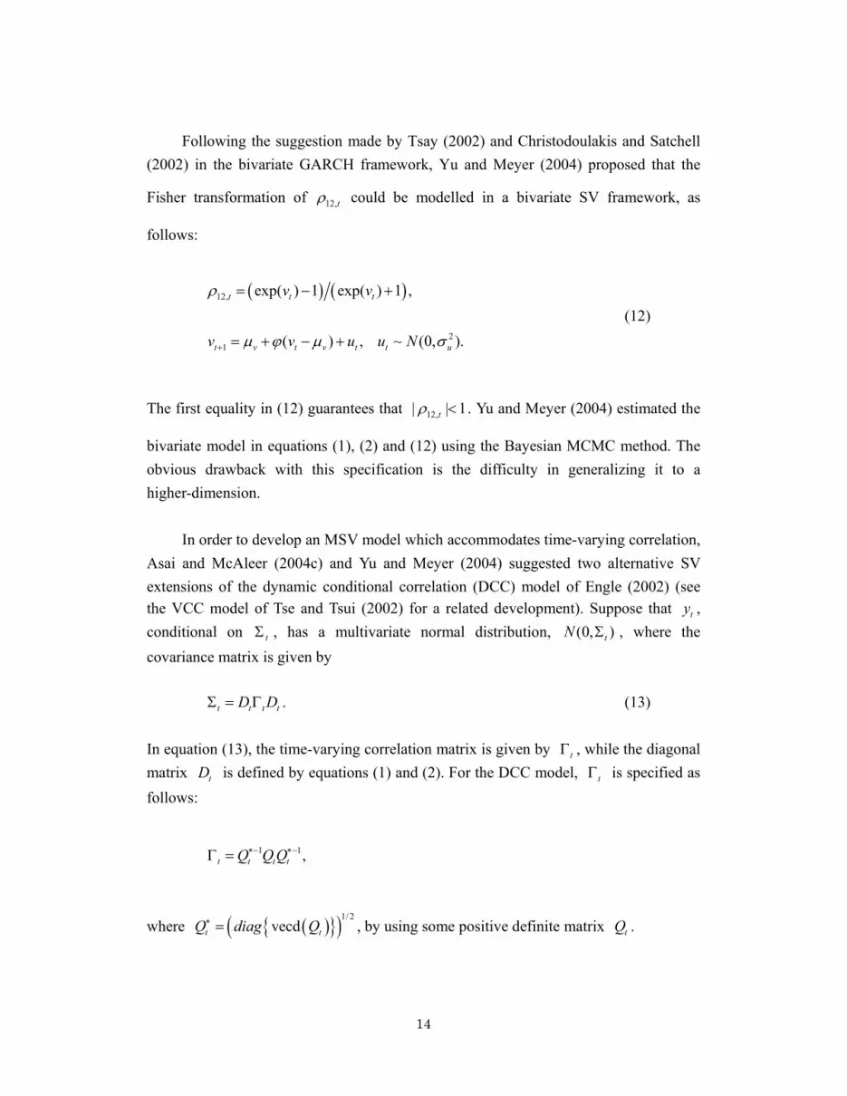
Following the suggestion made by Tsay (2002) and Christodoulakis and Satchell (2002) in the bivariate GARCH framework, Yu and Meyer (2004) proposed that the

Fisher transformation of 12,tρ could be modelled in a bivariate SV framework, as

follows:

( ) ( )12,

21

exp( ) 1 exp( ) 1 ,

( ) , ~ (0, ).

t t t

t v t v t t u

v v

v v u u N

ρ

µ ϕ µ σ+

= − +

= + − +

(12)

The first equality in (12) guarantees that 12,| | 1tρ < . Yu and Meyer (2004) estimated the

bivariate model in equations (1), (2) and (12) using the Bayesian MCMC method. The obvious drawback with this specification is the difficulty in generalizing it to a higher-dimension.

In order to develop an MSV model which accommodates time-varying correlation, Asai and McAleer (2004c) and Yu and Meyer (2004) suggested two alternative SV extensions of the dynamic conditional correlation (DCC) model of Engle (2002) (see the VCC model of Tse and Tsui (2002) for a related development). Suppose that ty , conditional on tΣ , has a multivariate normal distribution, (0, )tN Σ , where the covariance matrix is given by

t t t tD DΣ = Γ . (13) In equation (13), the time-varying correlation matrix is given by tΓ , while the diagonal matrix tD is defined by equations (1) and (2). For the DCC model, tΓ is specified as follows:

1 1,t t t tQ Q Q∗− ∗−Γ =

where ( ) ( )1/ 2vecdt tQ diag Q∗ = , by using some positive definite matrix tQ .

15

Asai and McAleer (2004c) extended the DCC model by specifying tQ as follows:

1 (1 ) ,

~ ( , ),

t t t

t m

Q Q Q

W

ψ ψ

ν

+ = − + +Ξ

Ξ Λ (14)

where ),( ΛνmW denotes a Wishart distribution. This dynamic correlation MSV model

guarantees the positive definiteness of tΓ under the assumption that Q is positive

definite and | | 1ψ < . The latter condition also implies that the time-varying correlations are mean reverting. In the special case where 1ν = , tΞ can be expressed as the cross-product of a multivariate normal variate with mean zero and covariance matrix given by Λ .

Yu and Meyer (2004) proposed an alternative MSV extension of DCC by specifying tQ as follows:

1 ( ) ( )

( ) ,

t t t t

t t t

Q S B Q S A e e S

S A B B Q A e eιι

+ ′= + − + −

′ ′= − − + +

o o

o o o

(15)

where ~ (0, )t me N I . According to Ding and Engle (2001) and Engle (2002), if A , B and ( )A Bιι′ − − are positive semi-definite, then tQ will also be positive semi-definite. Moreover, if any one of the matrices is positive definite, then tQ will also be positive definite. 2.5 Alternative Specifications This sub-section introduces four alternative MSV models based on the matrix exponential transformation, the Cholesky decomposition, the Wishart autoregressive process, and the observed range, respectively. 2.5.1 Matrix Exponential Transformation

16

Chiu et al. (1996) proposed a general framework for the logarithmic covariance matrix based on the matrix exponential transformation, which is well known in the mathematics literature (see, for example, Bellman (1970)). In this sub-section, we denote Exp(.) as the matrix exponential operation to distinguish it from the standard exponential operation. For any m m× matrix A , the matrix exponential transformation is defined by the power series expansion:

0

Exp( ) (1/ !) ,S

s

A s A∞

=

=∑ (16)

where 0A reduces to the m m× identity matrix and sA denotes the standard matrix multiplication of A s times. Thus, in general, the elements of Exp( )A do not typically exponentiate the elements of A .

The properties of the matrix exponential and matrix logarithm are summarized in Chiu et al. (1996). For any real symmetric matrix A , we note the singular value decomposition A TDT ′= , where the columns of the m m× orthonormal matrix T denote the appropriate eigenvectors of A , and D is an m m× diagonal matrix, with elements equal to the eigenvalues of A . Therefore, Exp( ) Exp( )A T D T ′= , where Exp( )D is an m m× diagonal matrix, with diagonal elements equal to the exponential of the corresponding eigenvalues of A . If it is assumed that Exp( )t tAεΣ = for any symmetric matrix tA , then tΣ is positive definite.

Similarly, the matrix logarithmic transformation, Log( )B , for any m m×

positive definite matrix, B , is defined by using the spectral decomposition of B .

Using the matrix exponential operator, we propose the following model:

~ (0, ),

Exp( ),

t t

t t

y N

A

Σ

Σ = (17)

where vech( )t tAα = is a vector autoregressive process, as follows:

17

1 ,

~ (0, ),

t t t t

t

x

N η

α µ φ α η

η

+ = + ϒ + +

Σ

o

(18)

with ( ),| |t t tx y y ′′ ′= , n×1 parameter vectors µ and φ , where n = 0.5m(m+1), n n×

covariance matrix ηΣ , and an 2n m× matrix of parameters ϒ . A limitation of this

specification is that it is not straightforward to interpret the relationship between the elements of tΣ and tA . 2.5.2 Cholesky Decomposition One of the most serious difficulties in modelling multivariate volatility is to ensure that the covariance matrix is positive semi-definiteness (see, for example, Engle and Kroner (1995)). Although the conventional approach is to impose suitable parametric restrictions, Tsay (2002) advocated an alternative approach, which uses the Cholesky decomposition. For a symmetric, positive-definite matrix tΣ , the Cholesky

decomposition factors the matrix tΣ uniquely in the form 'tttt LGL=Σ , where tL is a

lower triangular matrix with unit diagonal elements, and tG is a diagonal matrix with positive elements.

The MSV model of Tsay (2002) is given as follows:

18

'

21,

1, 2,

11, , 1

1

, 1 , ,

| ~ (0, ),

,

1 0 01 0

,

1

, , exp( ), ,exp( ),

, 1, , ,

, .

t t t

t t t t

tt

m t m t

t t mm t t mt

it i i it it

ij t ij ij ij t ij t

y N

L G L

qL

q q

G diag g g diag h h

h h i m

q q u i j

µ φ η

α β

+

+

Σ Σ

Σ =

=

= =

= + + =

= + + >

L

L

M M M M

L

K K

K

The elements in tG are always positive due to the exponential transformation. Consequently, the Cholesky decomposition guarantees the positive semi-definiteness of

tΣ . It can be seen that the elements in tL and tG are assumed to follow an AR(1) process. Moreover, it is straightforward to derive the relationship between the variances and correlations, on the one hand, and the variables in tL and tG , on the other, as follows:

2, , ,

1

, , , ,1

, , ,, 1

,, , 2 2

, , , ,1 1

, 1, , ,

, , 2, , ,

.

i

ii t ik t kk tk

j

ij t ik t jk t kk tk

j

ik t jk t kk tij t k

ij t jiii t jj t

ik t kk t jk t kk tk k

q g i m

q q g i j i m

q q g

q g q g

σ

σ

σρ

σ σ

=

=

=

= =

= =

= > =

= =

∑

∑

∑

∑ ∑

K

K

It is clear from these expressions that the dynamics in tiig , and tijq , are the

19

driving forces underlying the time-varying volatility and the time-varying correlation. However, the dynamics underlying volatility are not determined separately from those associated with the correlations, as both are dependent on their corresponding AR(1) processes. This restriction is, at least in spirit, similar to that associated with factor MSV models. 2.5.3 Wishart Autoregressive Models Gourieroux et al. (2004) proposed the Wishart autoregressive (WAR) multivariate process of stochastic positive semi-definite matrices to develop an altogether different type of dynamic MSV model. Let tΣ denote a time-varying covariance matrix of ty . Gourieroux et al. (2004) defined the WAR( p ) process, as follows:

∑=

=ΣK

kktktt xx

1

' (19)

where 1−> mK and each ktx follows the VAR( p ) model, given by:

,1

, (0, )p

kt i k t i kt kti

x A x Nε ε−=

= + Σ∑ .

By using the realized value of volatility, Gourieroux et al. (2004) estimated the parameters of the WAR(1) process using a two-step procedure based on nonlinear least squares.

Philipov and Glickman (2004b) suggested an alternative model based on Wishart processes, as follows:

11 1

| ~ (0, ),

| , ~ ( , ),

t t t

t t m t

y N

S W Sν ν−− −

Σ Σ

Σ

(20)

where ν and tS are the degrees of freedom and the time-dependent scale parameter of the Wishart distribution, respectively. With a time-invariant covariance structure, the above model may be considered as a traditional Normal-Wishart representation of the

20

behavior of multivariate returns. However, Philipov and Glickman (2004b) introduced time variation in the scale parameter, as follows:

( )( ) ( )1/ 2 1 1/ 21 d

t tS A Aν

−= Σ ,

where A is a positive definite symmetric parameter matrix that is decomposed through

a Cholesky decomposition as ( )( )1/ 2 1/ 2A A A ′= , and d is a scalar parameter. The

quadratic expression ensures that the covariance matrices are symmetric positive definite. Philipov and Glickman (2004b) estimated the parameters of the above model using the Bayesian MCMC technique. 2.5.4 Range-Based Model Tims and Mahieu (2003) proposed a range-based MSV model. As the range can be used as a measure of volatility, which is observed (or realized) when the high and low prices are recorded, Tims and Mahieu (2003) suggested a multivariate model for volatility directly, as follows:

1

log( ) ' , ~ (0, ),

, ~ (0, ).

t t t t

t t t t

range D f N

f f N η

ε ε

η η+

= + Σ

= Φ + Σ

As the volatility is not latent in this model, efficient estimation of the parameters is achieved through the use of the Kalman filter. It is not known, however, how to use this model for purposes of asset pricing. 3. Estimation As SV models typically do not have a closed-form expression for the likelihood function, the estimation of the parameters for the wide range of univariate and multivariate SV models has attracted significant attention in the literature.

An important concern for the choice of a particular estimation method lies in its

21

efficiency. In addition to efficiency, other important issues related to estimation include: (1) estimation of the latent volatility; (2) determination of the optimal filtering, smoothing and forecasting methods; (3) computational efficiency; (4) applicability for flexible modelling. Broto and Ruiz (2004) provided a recent survey regarding the numerous estimation techniques for SV models, with an emphasis on univariate SV models and methods. Some of these techniques have also been applied to the estimation of MSV models. 3.1 Quasi-Maximum Likelihood In order to estimate the parameters of the model (1)-(3), Harvey et al. (1994) proposed a Quasi-Maximum Likelihood (QML) method based on the property that the transformed

vector 2 21(ln , , ln )t t mty y y∗ ′= K has a state space form with the measurement equation

given by:

2 2 21

,

ln (ln , , ln )

t t t

t t t mt

y h ξ

ξ ε ε ε

∗ = +

′= = K

(21)

and the transition equation (2). The measurement equation errors, tξ , are non-normal, with mean vector ( ) 1.2793tE ξ ι= − , where ι is an 1m× vector of unit elements.

Harvey et al. (1994) showed that the covariance matrix of tξ , denoted ξΣ , is given by

2( / 2) ijξ π ρ∗Σ = , where 1iiρ∗ = and

22

1

2 ( 1)! ,(1/ 2)

nij ij

n n

nn

ρ ρπ

∞∗

=

−= ∑ (22)

where ( ) ( 1) ( 1)nx x x x n= + + −L and ijρ is defined by (3). Treating tξ as a

Gaussian error term, QML estimates may be obtained by applying the Kalman filter to equations (2) and (21). Taking account of the non-normality in tξ , the asymptotic standard errors can be obtained by using the results established in Dunsmuir (1979).

22

If ijρ∗ can be estimated, then it is also possible to estimate the absolute value of

ijρ , and the cross-correlations between the different values of itε . Estimation of the

signs of ijρ may be obtained by returning to the untransformed observations, and

noting that the sign of each of the pairs, it jtε ε ( , 1, ,i j m= K ), will be the same as the

corresponding pairs of observed values, it jty y . Therefore, the sign of ijρ is estimated

as positive if more than one-half of the pairs, it jty y , is positive.

One of the main features of this transformation is that tξ and tη are uncorrelated

even if the original tε and tη are correlated (see Harvey et al. (1994)). Since the

leverage effects assume a negative correlation between tε and tη , as in equation (5),

the transformation may ignore the information regarding the leverage effects. In the

univariate case, Harvey and Shephard (1996) recovered it in the state space form, given

the signs of the observed values. As for the multivariate case, Asai and McAleer

(2004b) derived the state space form for the leverage effects in the model (1), (2) and

(5), based on pairs of the signs of ity and jty . This representation enables use of the

QML method based on the Kalman filter. However, Asai and McAleer (2004b) adopted

the Monte Carlo likelihood method for purposes of efficient estimation.

The main advantages of the QML method are that it is computationally convenient,

and also straightforward for purposes of filtering, smoothing, and forecasting.

Unfortunately, the available (though limited) Monte Carlo experiments in the context of

the basic univariate SV model suggest that the QML method is generally less efficient

than the Bayesian MCMC technique and the likelihood approach based on Monte Carlo

simulation (for further details, see Jacquier et al. (1994) and the discussions contained

therein). It is natural to believe that inefficiency remains for the QML method relative to

the Bayesian MCMC technique and the likelihood approach in the multivariate context,

23

although no Monte Carlo evidence is available to date.

3.2 Simulated Maximum Likelihood

One Simulated Maximum Likelihood (SML) method is the Accelerated Gaussian Importance Sampling (AGIS) approach, as developed in Danielsson and Richard (1993). The AGIS approach is designed to estimate dynamic latent variable models, whereby Monte Carlo methods are used to integrate the latent variables out of the joint density of the latent and observable variables to obtain the marginal densities of the observable variables. Danielsson’s comments on Jacquier et al. (1994) show that the finite sample property of this SML estimator is close to that of the Bayesian MCMC method. As for MSV models, Danielsson (1998) applied the AGIS approach to estimate the parameters of the MSV model in (1)-(3). It seems difficult to extend the AGIS approach to accommodate more flexible SV models, as the method is specifically designed for models with a latent Gaussian process.

While the AGIS technique has limited applicability, the Efficient Importance

Sampling (EIS) procedure proposed by Richard and Zhang (2004), and applied by Liesenfeld and Richard (2003, 2004), is applicable to models with more flexible classes of distributions for the latent variables. As in the case of AGIS, EIS is a Monte Carlo technique for the evaluation of high-dimensional integrals. The EIS relies on a sequence of simple low-dimensional least squares regressions to obtain a very accurate global approximation of the integrand. This approximation leads to a Monte Carlo sampler, which produces highly accurate Monte Carlo estimates of the likelihood. In order to estimate the parameters of the additive factor model (10) with one factor, Liesenfeld and Richard (2003) proposed an SML approach by approximating the likelihood function based on EIS, while Liesenfeld and Richard (2004) developed a multi-move MCMC algorithm by sampling the latent variables based on EIS.

Let tλ denote a q -dimensional vector of latent variables, and ( , ; )f Y θΛ be the

joint density of 1

Tt t

Y y=

= and 1

Tt tλ

=Λ = . The likelihood function associated with

the observable variables, Y , is given by the ( )T q× -dimensional integral

( ; ) ( , ; )L Y f Y dθ θ= Λ Λ∫ . The likelihood function can be factorized as:

24

1 1 1 1 11 1( ; ) ( , | , , ) ( | , , ) ( | , , ) ,T T

t t t t t t t t t tt tL Y f y Y d g y Y p Y dθ λ θ λ θ λ θ− − − − −= =

= Λ Λ = Λ Λ∏ ∏∫ ∫

where 1

tt s s

Y y=

= and 1

tt s s

λ=

Λ = . It should be noted that the second equality

implies that ty is independent of 1t−Λ , given 1( , )t tYλ − , which is a standard assumption in the analysis of SV models. Although it is assumed, for notational convenience, that the initial values 0 1 , , y y− K and 0 1 , , λ λ− K are known constants, this condition can be relaxed. A Monte Carlo estimate of ( ; )L Yθ based on the above factorization is given by:

( )1

1 1

1ˆ( ; ) ( | ( ), , )TN

it t t

i t

L Y g y YN

θ λ θ θ−= =

=

∑ ∏ % ,

where the ( )

1( )

Tit tλ θ

=% are samples drawn from the conditional density

( )1 11( | , , )i

t t ttp Yλ θ− −−Λ% . This Monte Carlo estimate is inefficient in the sense that ( ) ( )itλ θ%

has no relation to the actual value tλ as it does not use any information about ty to

generate ( ) ( )itλ θ% from ( )

1 11( | , , )it t ttp Yλ θ− −−Λ% .

In order to cope with this problem, the AGIS proposed by Danielsson and Richard

(1993) and Danielsson (1994), and the EIS suggested by Richard and Zhang (2004), consider an auxiliary sampler, 1( | , )t t tm aλ −Λ . These methods enable the factorization given above to be rewritten as:

1 11

1 11

( , | , , )( ; ) ( | , ) ,( | , )

T Tt t t t

t t tt tt t t

f y YL Y m a dm aλ θθ λλ

− −−

= =−

Λ= Λ Λ Λ ∏ ∏∫

which yields an importance sampling Monte Carlo estimate, as follows:

( ) ( )

1 1 1( ) ( )

1 1 1 1

( , ( ) | , ( ), )1( ; ) ,( ( ) | ( ), )

i iTNt t t t t t

i ii t t t t t t

f y a Y aL YN m a a a

λ θθλ

− − −

= = − −

Λ= Λ

∑ ∏% %

%% %

(23)

25

where the ( )

1( )

Tit t t

aλ=

% are samples drawn from importance density ( )1( | , )i

t t tm aλ −Λ% .

The EIS method denotes an approximation of the density 1 1( , | , , )t t t tf y Yλ θ− −Λ as

( ; )t taκ Λ , and constructs the auxiliary density 1( | , )t t tm aλ −Λ , as follows:

11

( ; )( | , ) ,( ; )

t tt t t

t t

am aa

κλχ−

−

ΛΛ =

Λ

where 1( ; ) ( ; )t t t t ta a dχ κ λ−Λ = Λ∫ . It should be noted that matching

1 1( , | , , )t t t tf y Yλ θ− −Λ with ( ; )t taκ Λ may leave 1( ; )t taχ −Λ unexplained. As

1( ; )t taχ −Λ does not depend on tλ , it can be transferred back to the period 1t − minimization sub-problem. Taken together, EIS requires solving a simple back-recursive sequence of low-dimensional least squares problems of the form:

( ) ( )

( )

( ) ( ) ( )1 1 1

1

( )1

ˆ ˆarg min log , ( ) | , ( ), ( );

ˆ log ( );

t

Ni i i

t t t t t t ta i

it t t

a f y Y a

c a

λ θ θ θ χ θ

κ θ

− − +=

+

= Λ ⋅ Λ

− − Λ

∑ % %

%

for : 1t T → , with 1( ; ) 1T Taχ +Λ ≡ . The tc are unknown constants to be estimated jointly with the unknown ta . In order to obtain highly efficient importance samplers, a small number of iterations of the EIS algorithm is required. When such iterations converge to fixed values of the auxiliary parameters, ˆta , this would be expected to produce optimal importance samplers. Finally, the EIS estimate of the likelihood

function for a given value of θ is obtained by substituting 1ˆ T

t ta

= for 1

Tt t

a=

in

equation (23).

Moreover, the EIS method can be used to compute the filtered estimates of the latent variables. Let ( )th λ denote a function such as, for example, exp( )tλ , which represents the conditional return variance. Then the sequence of conditional expectations of ( )th λ , given 1tY − , the past observations of the returns, provides a sequence of filtered estimates of ( )th λ . For the SV model, these expectations take the

26

form of a ratio of integrals, as follows:

[ ] 1 1 1 11

1 1 1

( ) ( | , , ) ( , ; )( ) | ,

( , ; )t t t t t t t

t tt t t

h p Y f Y dE h Y

f Y d

λ λ θ θλ

θ− − − −

−− − −

Λ Λ Λ=

Λ Λ∫

∫

in which both the numerator and denominator can be estimated by the EIS algorithm.

In the application of the Bayesian MCMC method, Liesenfeld and Richard (2004) proposed using a combination of the EIS-sampler with Tierney's (1994) Acceptance-Rejection Metropolis-Hastings (AR-MH) algorithm to simulate | ,Y θΛ . The basis of such a procedure is the fact that the EIS density for Λ provides a very close approximation to ( | , )f Y θΛ .

3.3 Monte Carlo Likelihood

The Monte Carlo likelihood (MCL) approach for non-Gaussian models is based on importance sampling techniques, so that the method may be classified as an SML method. The MCL method can approximate the likelihood function to an arbitrary degree of accuracy by decomposing it into a Gaussian part, which is constructed by the Kalman filter, and a remainder function, whose expectation is evaluated through simulation.

Durbin and Koopman (1997) demonstrated that the log-likelihood function of state space models with non-Gaussian measurement disturbances could be expressed simply as

( | )ln ( | ) ln ( | ) ln ,

( | , )G GG

pL y L y E

p yξ ξ θ

θ θξ θ

= +

(24)

where 1( , ) 'Ty y y= K , 1( , ) 't t mty y y= K , and 1( , , ) 'Tξ ξ ξ= K and ln ( | )GL y θ are the vectors of measurement disturbances and the log-likelihood function of the

approximating Gaussian model, respectively, ( | )pξ ξ θ is the true density function,

( | , )Gp yξ θ is the Gaussian density of the measurement disturbances of the

27

approximating model, and GE refers to the expectation with respect to the ‘so-called’ importance density ( | , )Gp yξ θ associated with the approximating model. Equation (24) shows that the non-Gaussian log-likelihood function can be expressed as the log-likelihood function of the Gaussian approximating model plus a correction for the departures from the Gaussian assumptions relative to the true model.

A key feature of the MCL method is that only the minor part of the likelihood function requires simulations, unlike other SML methods. Therefore, the method is computationally efficient in the sense that it needs only a small number of simulations to achieve the desirable accuracy for empirical analysis.

The MCL estimates of the parameters, θ , are obtained by numerical optimization of the unbiased estimate of equation (24). The log-likelihood function of the approximating model, ln ( | )GL y θ , can be used to obtain the starting values. Sandmann and Koopman (1998) is the first paper to have used this MCL approach in the SV literature. Asai and McAleer (2004b) developed the MCL method for asymmetric MSV models. As noted in Asai (2004), this MCL method is also able to accommodate the additive factor MSV model.

3.4 Markov Chain Monte Carlo

Markov Chain Monte Carlo (MCMC) methods are used widely in the SV literature,

following the development in Jacquier et al. (1994), which has been greatly refined and

simplified by Shephard and Pitt (1997) and Kim et al. (1998). The idea behind MCMC

methods is to produce variates from a given multivariate density (the posterior density

in Bayesian applications) by repeatedly sampling a Markov chain whose invariant

distribution is the target density of interest. The MCMC method focuses on the density ( , | )h yπ θ instead of the usual posterior density, ( | )yπ θ , since the latter requires

computation of the likelihood function ( | ) ( | , ) ( | )f y f y h f h dhθ θ θ= ∫ . The MCMC

procedure only requires alternating back and forth between drawing from ( | , )f h yθ

and ( | , )f h yθ . This process of alternating between conditional distributions produces

a cyclic chain.

28

As for the property of sample variates from an MCMC algorithm, they are a

high-dimensional sample from the target density of interest. These draws can be used as

the basis for drawing inferences by appealing to suitable ergodic theorems for Markov

chains. For example, posterior moments and marginal densities can be estimated (or

simulated consistently) by averaging the relevant function of interest over the sampled

variates. The posterior mean of θ is estimated simply as the sample mean of the

simulated θ values. These estimates can be made arbitrarily accurate by increasing the

simulation sample size.

One particularly important technical advantage of the Bayesian MCMC method

over classical inferential techniques is that MCMC does not need to use numerical

optimization. This advantage becomes especially important when the number of

parameters to be estimated is large, as in the application of MSV models to the analysis

of financial data.

Jacquier et al. (1999), Pitt and Shephard (1999a), and Aguilar and West (2000)

have applied the MCMC procedure to estimate additive factor MSV models, while Yu and Meyer (2004) compared various MSV models. Moreover, Yu and Meyer (2004) employed the purpose-built Bayesian software package called BUGS (Bayesian Analysis Using the Gibbs Sampler). Each of these MCMC algorithms is based on a single-move algorithm.

The main drawback with the single-move algorithm for MSV models lies in its

slow convergence. This is not surprising since the components of the latent volatility process are highly persistent (Kim et al. (1998)). In order to improve the simulation efficiency, Chib et al. (2005) developed a new MCMC algorithm which greatly improves simulation efficiency for a factor MSV model augmented with jumps. Liesenfeld and Richard (2004) proposed an alternative multi-move MCMC method based on EIS, which can be used to estimate SV models by maximum likelihood, as well as simulation smoothing.

Bos and Shephard (2004) modelled the Gaussian errors in the standard Gaussian,

linear state space model as an SV process, and showed that conventional MCMC algorithms for this class of models are ineffective. Rather than sampling the unobserved

29

variance series directly, Bos and Shephard (2004) sampled in the space of the disturbances, which decreased the correlation in the sampler and increased the quality of the Markov chain. Using the reparameterized MCMC sampler, they showed how to estimate an unobserved factor model.

Smith and Pitts (2005) used a bivariate SV model to measure the effects of

intervention in stabilization policy. Missing observations were accommodated in the model and a data-based Wishart prior for the precision matrix of the errors in the transition equation were suggested. A threshold model for the transition equation was estimated by MCMC jointly with the bivariate SV model. 4. Diagnostic Checking and Model Comparison

Pitt and Shephard (1999a) conducted diagnostic checking which is applicable to the

MSV models. Although their method is based on the particle filter algorithm (Pitt and

Shephard (1999b)), other simulation filtering techniques, such as the EIS filter of

Liesenfeld and Richard (2003) and the reprojection technique of Gallant and Tauchen

(1998), may also be applicable. By using these filtering methods, we can obtain samples from the prediction density, 1( | ; )t tf h Y θ+ , where 1( , , )t tY y y ′= K . Pitt and Shephard

(1999a) focus on four quantities for assessing overall model fit, outliers and

observations which have substantial influence on the fitted model.

The first quantity is the log-likelihood for 1t + , 1 1log ( | ; )t t tl f y Y θ+ += . As we

have the following:

1 1 1 1( | ; ) ( | ; ) ( | ; )t t t t t tf y Y f y h dF h Yθ θ θ+ + + += ∫ ,

Monte Carlo integration may be used as

1 1 11

1ˆ ( | ; ) ( | ; ),M

it t t t

i

f y Y f y hM

θ θ+ + +=

= ∑

30

where 1 1~ ( | ; )it t th f h Y θ+ + . It is possible to evaluate the log-likelihood at the ML (MCL,

SML) estimates or at the posterior means.

The second quantity is the normalized log-likelihood, ntl . Pitt and Shephard

(1999a) used samples from jz ( 1, ,j S= K ), where 1~ ( | ; )jt tz f y Y θ+ , to obtain

samples 1itl + using the above method. Denote the sample mean and standard deviation

of the samples of log-likelihood as 1ltµ + and 1

ltσ + , respectively. The normalized

log-likelihood at 1t + may be computed as ( )1 1 1 1n l lt t t tl l µ σ+ + + += − . If the model and

parameters are correct, then this statistic should have mean zero and variance one. Large

negative values indicate that an observation is less likely than would be expected from

the model.

The third quantity is the uniform residual, 1 1( | ; )t t tu F l Y θ+ += , which may be

estimated as

( )1 1 1 11ˆˆ ( ) 1 ( )S j

t t t tju F l S I l l+ + + +=

= = <∑ ,

where the 1j

tl + are constructed as above. Assuming that the parameter vector θ is

known, under the null hypothesis that the model is correct, it follows that

1ˆ ~ (0,1)tu UID+ .

Finally, the fourth quantity is the distance measure, td , which may be computed

as follows:

( )1 1 1 11( | ; ) 1 ( | ; )M i

t t t t tiV y Y M V y hθ θ+ + + +=

Σ = ∑ ,

31

where 1 1~ ( | ; )it t th f h Y θ+ + . If the conditional distribution of ty is multivariate normal,

then the quantity 1t t t td y y−′= Σ is independently distributed as 2

mχ under the null

hypothesis that the parameters and model are correct. Therefore, we may use

21

~Tt mTt

d χ=∑ as a test statistic.

When the MCMC procedure is used, it may require checking convergence of

Markov chains and prior sensitivities. The former can be assessed by correlograms, and

the latter by using alternative priors (for further details, see Kim et al. (1998), Chib

(2001) and Chib et al. (2005)).

Turning to model selection, we may use the likelihood ratio test for the nested

models, and Akaike information criterion (AIC) or Bayesian information criterion (BIC)

for the non-nested models, in the context of the likelihood-based methods, such as SML

and MCL. In the Bayesian framework, model comparison can be conducted via the

posterior odds ratio or Bayes factor. For both values, the marginal likelihood needs to be

calculated, for which estimation is based on the procedure proposed by Chib (1995) and

its various extensions.

The AIC is inappropriate for the MCMC method because, when MCMC is used to

estimate the SV models, as mentioned above, the parameter space is augmented. For

example, in the basic univariate SV model, we include the T latent volatilities in the

parameter space, with T being the sample size. As these volatilities are dependent,

they cannot be counted as T additional free parameters. Consequently, AIC is not

applicable for comparing SV models. Recently, Berg et al. (2004) showed that model

selection of alternative univariate SV models can be performed easily using the

deviance information criterion (DIC) proposed by Spiegelhalter et al. (2002), while Yu

and Meyer (2004) compared alternative MSV models using DIC.

32

5. Concluding Remarks As the literature on multivariate stochastic volatility (MSV) models has developed significantly over the last few years, this paper reviewed the substantial literature on specification, estimation and evaluation of MSV models. A wide range of MSV models was presented according to various categories, namely (i) asymmetric models; (ii) factor models; (iii) time-varying correlation models; and (iv) alternative MSV specifications, including models based on the matrix exponential transformation, Cholesky ecomposition, Wishart autoregressive process, and the empirical range. Alternative methods of estimation, including quasi-maximum likelihood, simulated maximum likelihood, Monte Carlo likelihood, and Markov chain Monte Carlo methods, were discussed and compared. Various methods of diagnostic checking and model comparison were also examined.

Relative to the extensive theoretical and empirical multivariate GARCH literature,

the MSV literature is still in its infancy. The majority of existing research in the MSV literature deals with specifications and/or estimation techniques, which are often illustrated by fitting a particular symmetric or asymmetric MSV model to financial returns series. Few papers have directly addressed important economic issues using MSV models. To our knowledge, Nardari and Scruggs (2003) and Han (2002) are two exceptions. Nardari and Scrugg used MSV models to address the restrictions in the APT theory while Han examined the economic values of MSV models. Clearly, further applications of MSV models are needed.

Most of the MSV models discussed in this paper have been estimated using at

most 3 or 4 return series. Chib et al. (2005) is the first paper in the literature where genuinely high-dimensional MSV models have been estimated. Chan et al. (2003) and Nadari and Scruggs (2003) also estimated high-dimensional MSV models. With the development of superior estimation techniques and the availability of greater computing power, the literature on specification, estimation and evaluation of high-dimensional MSV models will be broadened appreciably.

33

References Aguilar, O., and M. West (2000), “Bayesian Dynamic Factor Models and Portfolio Allocation”, Journal of Business and Economic Statistics, 18, 338-357. Andersen, T.G., T. Bollerslev, F.X. Diebold and P. Labys (2003), “Modelling and Forecasting Realized Volatility”, Econometrica, 71, 579-625. Asai, M. (2004), “A Comparative Analysis of Multi-Factor Stochastic Volatility Models with Heavy-Tailed Models and Higher-Order Autoregressive Models”, unpublished paper, Faculty of Economics, Tokyo Metropolitan University. Asai, M., and M. McAleer (2004a), “Dynamic Asymmetric Leverage in Stochastic Volatility Models”, unpublished paper, Faculty of Economics, Tokyo Metropolitan University. Asai, M., and M. McAleer (2004b), “Asymmetric Multivariate Stochastic Volatility”, unpublished paper, Faculty of Economics, Tokyo Metropolitan University. Asai, M., and M. McAleer (2004c), “Dynamic Correlations in Stochastic Volatility Models”, unpublished paper, Faculty of Economics, Tokyo Metropolitan University. Bauwens, L., S. Laurent and J.V.K. Rombouts (2004), “Multivariate GARCH: A Survey”, to appear in Journal of Applied Econometrics. Bellman, R. (1970), Introduction to Matrix Analysis, McGraw-Hill, New York. Berg, A., R. Meyer and J. Yu (2004), “Deviance Information Criterion for Comparing Stochastic Volatility Models”, Journal of Business and Economic Statistics, 22, 107-120. Black, F. (1976), “Studies of Stock Market Volatility Changes”, 1976 Proceedings of the American Statistical Association, Business and Economic Statistics Section, pp.177-181. Bollerslev, T. (1990), “Modelling the Coherence in Short-run Nominal Exchange Rates:

34

A Multivariate Generalized ARCH Approach”, Review of Economics and Statistics, 72, 498-505. Bollerslev, T., R.F. Engle and J. Wooldridge (1988), “A Capital Asset Pricing Model with Time Varying Covariance”, Journal of Political Economy, 96, 116–131. Bos, C.S and N. Shephard (2004), “Inference for Adaptive Time Series Models: Stochastic Volatility and Conditionally Gaussian State Space Form”, unpublished paper, Tinbergen Institute and Vrije Universiteit Amsterdam. Broto, C., and E. Ruiz (2004), “Estimation Methods for Stochastic Volatility Models: A Survey”, Journal of Economic Surveys, 18, 613-649. Campbell, J.Y., and L. Hentschel (1992), “No News is Good News: An Asymmetric Model of Changing Volatility in Stock Returns”, Journal of Financial Economics, 31, 281-318. Chan, D., R. Kohn and C. Kirby (2003), “Multivariate Stochastic Volatility with Leverage”, unpublished paper, School of Economics, University of New South Wales. Chesney, M., and L.O. Scott (1989), “Pricing European Currency Options: A Comparison of the Modified Black-Scholes Model and a Random Variance Model”, Journal of Financial and Quantitative Analysis, 24, 267-284. Chib, S. (1995), “Marginal Likelihood from the Gibbs Output”, Journal of the American Statistical Association, 90, 1313-1321. Chib, S. (2001), “Markov Chain Monte Carlo Methods: Computation and Inference”, in J.J. Heckman and E. Leamer (eds.), Handbook of Econometrics, Volume 5, North-Holland , pp. 3569–3649. Chib, S., F. Nardari and N. Shephard (2005), “Analysis of High Dimensional Multivariate Stochastic Volatility Models”, to appear in Journal of Econometrics. Chiu, T.Y.M, T. Leonard and K.-W. Tsui (1996), “The Matrix-Logarithmic Covariance Model,” Journal of the American Statistical Association, 91, 198-210.

35

Christie, A.A. (1982), “The Stochastic Behavior of Common Stock Variances: Value, Leverage and Interest Rate Effects”, Journal of Financial Economics, 10, 407-432. Christodoulakis, G., and S.E. Satchell (2002), “Correlated ARCH (CorrARCH): Modelling the time-varying conditional correlation between fianacial asset returns”, European Journal of Operational Research, 139, 351-370. Danielsson, J. (1994), “Stochastic Volatility in Asset Prices: Estimation with Simulated Maximum Likelihood”, Journal of Econometrics, 64, 375-400. Danielsson, J. (1998), “Multivariate Stochastic Volatility Models: Estimation and a Comparison with VGARCH Models”, Journal of Empirical Finance, 5, 155–173. Danielsson, J., and J.-F. Richard (1993), “Quadratic Acceleration for Simulated Maximum Likelihood Evaluation”, Journal of Applied Econometrics, 8, 153–173. Diebold, F.X., and M. Nerlove (1989), “The Dynamics of Exchange Rate Volatility: A Multivariate Latent-Factor ARCH Model”, Journal of Applied Econometrics, 4, 1 –22. Ding, Z., and R. Engle (2001), “Large Scale Conditional Covariance Modelling, Estimation and Testing”, Academia Economic Papers. 29, 157-184. Durbin, J., and S.J. Koopman (1997), “Monte Carlo Maximum Likelihood Estimation for Non-Gaussian State Space Models”, Biometrika, 84, 669-684. Dunsmuir, W. (1979), “A Central Limit Theorem for Parameter Estimation in Stationary Vector Time Series and Its Application to Models for a Signal Observed with Noise”, Annals of Statistics, 7, 490-506. Engle, R.F. (1982), “Autoregressive Conditional Heteroscedasticity with Estimates of the Variance of United Kingdom Inflation”, Econometrica, 50, 987-1007. Engle, R.F. (2002), “Dynamic Conditional Correlation: A Simple Class of Multivariate Generalized Autoregressive Conditional Heteroskedasticity Models,” Journal of Business and Economic Statistics, 20, 339-350.

36

Engle, R.F. and K.F. Kroner (1995), “Multivariate Simultaneous Generalized ARCH”, Econometric Theory, 11, 122-150. Engle, R., and V. Ng (1993), “Measuring and Testing the Impact of News in Volatility”, Journal of Finance, 43, 1749-1778. Engle, R.F., V. Ng, and M. Rothschild (1990), “Asset Pricing with a Factor-ARCH Covariance Structure,” Journal of Econometrics, 45, 213–237. Gallant, A.R., and G.E. Tauchen (1998), “Reprojecting Partially Observed Systems with Application to Interest Rate Diffusions”, Journal of the American Statistical Association, 93, 10- 24. Geweke, J., and S. Porter-Hudak (1983), “The Estimation and Application of Long Memory Time Series Models”, Journal of Time Series Analysis, 4, 221-238. Ghysels, E., A.C. Harvey and E. Renault (1996), “Stochastic Volatility”, in C.R. Rao and G.S. Maddala (eds.), Statistical Models in Finance, North-Holland, Amsterdam, pp. 119-191. Glosten, L., R. Jagannathan and D. Runkle (1993), “On the Relation Between the Expected Value and Volatility of Nominal Excess Returns on Stocks”, Journal of Finance, 46, 1779-1801. Gourieroux, C., J. Jasiak and R. Sufana (2004), “The Wishart Autoregressive Process of Multivariate Stochastic Volatility”, unpublished paper, CRES and CEPREMAP. Han, Y., (2002), “The Economics Value of Volatility Modelling: Asset Allocation with a High Dimensional Dynamic Latent Factor Multivariate Stochastic Volatility Model”, unpublished paper, Olin School of Business, Washington University in St. Louis. Harvey, A.C., E. Ruiz and N. Shephard (1994), “Multivariate Stochastic Variance Models”, Review of Economic Studies, 61, 247-264. Harvey, A.C. and N. Shephard (1996), “Estimation of an Asymmetric Stochastic

37

Volatility Model for Asset Returns”, Journal of Business and Economic Statistics, 14, 429-434. Hull, J., and A. White (1987), “The Pricing of Options on Assets with Stochastic Volatility”, Journal of Finance, 42, 281-300. Jacquier, E., N.G. Polson and P.E. Rossi (1994), “Bayesian Analysis of Stochastic Volatility Models (with discussion)”, Journal of Business and Economic Statistics, 12, 371– 389. Jacquier, E., N.G. Polson and P.E. Rossi (1995), “Models and Priors for Multivariate Stochastic Volatility”, CIRANO Working Paper No. 95s-18, Montreal. Jacquier, E., N.G. Polson and P.E. Rossi (1999), “Stochastic Volatility: Univariate and Multivariate Extensions”, CIRANO Working paper 99s-26, Montreal. Jacquier, E., N.G. Polson and P.E. Rossi (2004), “Bayesian Analysis of Stochastic Volatility Models with Fat-Tails and Correlated Errors”, Journal of Econometrics, 122, 185-212. Kim, S., N. Shephard and S. Chib (1998), “Stochastic Volatility: Likelihood Inference and Comparison with ARCH Models”, Review of Economic Studies, 65, 361-393. Liesenfeld, R., and J.-F. Richard (2003), “Univariate and Multivariate Stochastic Volatility Models: Estimation and Diagnostics”, Journal of Empirical Finance, 10, 505-531. Liesenfeld, R., and J.-F. Richard (2004), “Classical and Bayesian Analysis of Univariate and Multivariate Stochastic Volatility Models”, unpublished paper, Department of Economics, Christian-Albrecht-Universitat, Germany. McAleer, M. (2005), “Automated Inference and Learning in Modeling Financial Volatility”, Econometric Theory, 21, 232-261. Nardari, F., and J. Scruggs (2003), “Analysis of Linear Factor Models with Multivariate Stochastic Volatility for Stock and Bond Returns”, unpublished paper, Department of

38

Finance, Arizona State University. Nelson, D.B. (1991), “Conditional Heteroscedasticity in Asset Returns: A New Approach”, Econometrica, 59, 347-370. Philipov, A., and M.E. Glickman (2004a), “Factor Multivariate Stochastic Volatility Via Wishart Processes”, unpublished paper, Department of Health Services, Boston University. Philipov, A., and M.E. Glickman (2004b), “Multivariate Stochastic Volatility Via Wishart Processes”, unpublished paper, Department of Health Services, Boston University. Pitt, M., and N. Shephard (1999a), “Time Varying Covariances: A Factor Stochastic Volatility Approach”, in J.M. Bernardo, J.O. Berger, A.P. David and A.F.M. Smith (eds.), Bayesian Statistics 6, Oxford University Press, pp. 547-570. Pitt, M., and N. Shephard (1999b), “Filtering via Simulation: Auxiliary Particle Filter”, Journal of the American Statistical Association, 94, 590–599. Quintana, J.M., and M. West (1987), “An Analysis of International Exchange Rates Using Multivariate DLMs”, The Statistician, 36, 275-281. Ray, B.K., and R.S. Tsay (2000), “Long-range Dependence in Daily Stock Volatilities”, Journal of Business and Economic Statistics, 18, 254–262. Richard, J.-F., and W. Zhang (2004), “Efficient High-Dimensional Importance Sampling”, unpublished paper, Department of Economics, University of Pittsburg. Robinson, P.M. (1995), “Log-Periodogram Regression with Time Series with Long-Range Dependence”, Annals of Statistics, 23, 1048-1072. Sandmann, G. and S.J. Koopman (1998), “Estimation of Stochastic Volatility Models via Monte Carlo Maximum Likelihood”, Journal of Econometrics, 87, 271-301. Shephard, N. (1996), “Statistical Aspects of ARCH and Stochastic Volatility”, in D.R.

39

Cox, D.V. Hinkley and O.E. Barndorff-Nielsen (eds.), Time Series Models in Econometrics, Finance and Other Fields. Chapman & Hall, London, pp. 1-67. Shephard, N., and M.K. Pitt (1997), “Likelihood Analysis of Non-Gaussian Measurement Time Series”, Biometrika, 84, 653-667. Smith, M. and A. Pitts (2005), “Foreign Exchange Intervention by the Bank of Japan: Bayesian Analysis Using a Bivariate Stochastic Volatility Model”, unpublished paper, Econometrics and Business Statistics, University of Sydney. So, M.K.P., W.K. Li and K. Lam (2002), “A Threshold Stochastic Volatility Model”, Journal of Forecasting, 21, 473-500. Spiegelhalter, D.J., N.G. Best, B.P. Carlin and A. van der Linde (2002), “Bayesian Measures of Model Complexity and Fit (with discussion)”, Journal of the Royal Statistical Society, Series B, 64, 583-639. Taylor, S.J. (1982), “Financial Returns Modelled by the Product of Two Stochastic Processes ― A Study of the Daily Sugar Prices 1961-75”, in O.D. Anderson (ed.) Time Series Analysis: Theory and Practice, Vol. 1, North-Holland, pp.203-226. Taylor, S.J. (1986), Modelling Financial Time Series, Wiley, Chichester. Tierney, L. (1994), “Markov Chains for Exploring Posterior Distributions”, Annals of Statistics, 22, 1701-1762. Tims, B. and R. Mahieu (2003), “A Range-Based Multivariate Model for Exchange Rate Volatility”, unpublished paper, Department of Financial Management, Erasmus University Rotterdam. Tsay, R.S. (2002), Analysis of Financial Time Series: Financial Econometrics, Wiley, New York. Tse, Y.K., and A.K.C. Tsui (2002), “A Multivariate Generalized Autoregressive Conditional Heteroscedasticity Model with Time-Varying Correlations”, Journal of Business and Economic Statistics, 20, 351-362.

40

Wiggins, J.B. (1987), “Option Values Under Stochastic Volatility: Theory and Empirical Estimates”, Journal of Financial Economics, 19, 351-372. Yu, J. (2004a), “On Leverage in a Stochastic Volatility Model”, to appear in Journal of Econometrics. Yu, J. (2004b), “Asymmetric Response of Volatility: Evidence from Stochastic Volatility Models and Realized Volatility”, School of Economics and Social Sciences, Singapore Management University, Working Paper 24-2004. Yu, J., and R. Meyer (2004), “Multivariate Stochastic Volatility Models: Bayesian Estimation and Model Comparison”, School of Economics and Social Sciences, Singapore Management University, Working Paper 23-2004.