Fractal features for localization of temporal lobe epileptic foci using SPECT imaging

ARTICLE IN PRESS

Computers in Biology and Medicine 40 (2010) 469–477

Contents lists available at ScienceDirect

Computers in Biology and Medicine

0010-48

doi:10.1

� Corr

Docteur

E-m

journal homepage: www.elsevier.com/locate/cbm

Fractal features for localization of temporal lobe epileptic fociusing SPECT imaging

R. Lopes a,b, M. Steinling c,d, W. Szurhaj c,d, S. Maouche b, P. Dubois a,c,d, N. Betrouni a,c,d,�

a Inserm U703, Parc EuraSante, 152 rue du Docteur Yersin, 59120 Loos, Franceb CNRS UMR 8146, USTL, Batiment P2, Villeneuve d’Ascq, 59655, Francec Universite Lille Nord de France, F-59000 Lille, Franced CHU Lille, F-59000 Lille, France

a r t i c l e i n f o

Article history:

Received 6 May 2009

Accepted 4 March 2010

Keywords:

Epilepsy

SPECT

SISCOM

Detection

Fractal

Multifractal

Texture

SVM

25/$ - see front matter & 2010 Elsevier Ltd. A

016/j.compbiomed.2010.03.001

esponding author at: Inserm U703, Institu

Yersin, 59120 Loos, France. Tel.: +33 320 44

ail address: [email protected] (N. Betro

a b s t r a c t

Single photon emission computed tomography (SPECT) is an accurate imaging method for the diagnosis

of refractory partial epilepsy. Two scans are carried out: interictal and ictal. The interest of this method is

to provide an image in the ictal period, which allows hyperperfused areas linked to the seizure to be

localized. The epileptic foci localization is improved by subtracting the two acquisitions (subtracted ictal

SPECT: SIS). In some cases, the SIS method is not effective and does not isolate the seizure foci. In this

article, we investigate a new method based on texture analysis using fractal geometry features. Fractal

geometry features were extracted from each scan in order to quantify the heterogeneity change resulting

from the hyperperfusion. A support vector machine (SVM) classification algorithm was used to classify

the voxels into two classes: focal and healthy. Quantitative evaluation was performed on simulated

images and clinical images from 22 patients with temporal lobe epilepsy. Results on both experiments

showed that the proposed method is more specific and more sensitive than the SIS method.

& 2010 Elsevier Ltd. All rights reserved.

1. Introduction

Single photon emission computed tomography (SPECT) is anuclear medicine imaging method that allows the cerebralmetabolism to be studied. The most promising clinical applicationof SPECT in epilepsy is for the lateralizing of temporal lobe foci inpreparation for possible surgery [1]. The potential benefits aregreat if SPECT can provide reliable lateralization even in only somepatients with temporal lobe epilepsy [2]. Electrophysiologicallateralization, however, may be time-consuming. In temporal lobeepilepsy (TLE), interictal SPECT typically displays hypoperfusion inthe epileptogenic zones (EZ) in around 40–50% of cases [3] whenthe radiotracer is injected during the seizure. SPECT has beenclearly shown to be highly sensitive in detecting hyperperfusionon the ictal image [3,4]. The subtraction of interictal from ictalSPECT data coregistered to 3D-MRI (SISCOM) (or just SIS when noregistration of anatomical data is done) [5] makes the localizationof the EZ more precise. This routine technique is very useful inpresurgical evaluation of TLE [6,7], but in some cases it is notsensitive enough. A more sensitive method, which could detectslight changes of local metabolism not detected by visual analysisor the SISCOM method, is therefore required.

ll rights reserved.

t Hippocrate, 152, rue du

6 722; fax: +33 320 446 715.

uni).

Texture is a fundamental characteristic in many natural imagesand plays an important role in computer vision and patternrecognition. For this reason, many approaches to texture analysishave been investigated over the past two decades, especially inmedical image analysis. Fractal geometry has recently emerged asa new method. After initial applications which mainly focused onthe discrimination between two states (healthy versus pathologi-cal, for example), further investigation has examined the useful-ness of this geometry in the detection of textural heterogeneities[8,9]. Two analysis tools, fractal and multifractal, are used. Fractalanalysis provides an overall measure of the signal’s heterogeneityand texture via the estimation of the fractal dimension (FD). It isthe most widely used feature, but it is unable to distinguishbetween key textures, such as edges and corners. In contrast,multifractal analysis provides local characterization of the hetero-geneity via the estimation of the Holder coefficient [10]; it candistinguish between key textures.

The aim of this study was to investigate the benefit of thecombined use of 3D local fractal and multifractal features in thedetection of TLE foci on SPECT images.

2. Methods

Firstly, we introduce the fractal features. We then present thedetection method based on these features, combined with othertexture features.

www.elsevier.com/locate/cbm

dx.doi.org/10.1016/j.compbiomed.2010.03.001

mailto:[email protected]

ARTICLE IN PRESS

R. Lopes et al. / Computers in Biology and Medicine 40 (2010) 469–477470

2.1. Fractal geometry features

2.1.1. 3D fractal features

One of the difficulties in using fractal analysis is the choice ofthe computation algorithm. Many methods have been proposedfor FD calculation. Each method has its own theoretical basis, andthis often leads to different dimensions being obtained for thesame feature according to the method used. However, althoughthe applied algorithms are different, they all follow the same basicplan, summarized by the next three steps:

�
measurement of the number of elementary objects (with adefined size) needed to recover the image; � plotting of the curve log (measured quantities) versus log (step
sizes) and fitting a least squares regression line through thedata points;
� estimation of FD as the slope of the regression line.
The algorithms are grouped into three classes: ‘‘box counting’’,‘‘fractional Brownian motion’’ (the ‘‘variance’’ method) and‘‘perimeter-area measurement’’ (the blanket method).

To evaluate the ability of these methods to detect changes intexture when they are applied locally, we selected one method fromeach class. Thus, three FD values were extracted for each voxel.

‘‘Piecewise modified box counting’’ (PMBC) method: The PMBCmethod is a ‘‘box-counting’’ method; it requires decomposition ofthe elementary sub-images of the studied image. Zook et al. [11]introduced this method to calculate the FD for sub-images in 2Dimages. We here propose a scheme to implement the method for3D images. FD was calculated for each voxel as follows:

First, we divided the 3D image into 3D sub-images. Each sub-image was then divided into boxes of sizes d�d�d, and thedifference between the maximum and the minimum gray levelvalues was evaluated for each box. The sum of the differences wascalculated for the entire sub-image. Finally, the FD was estimated asthe slope of the linear fit of log (sum of differences) against log(d).

‘‘Variance’’ method: The variance method is based on thefractional Brownian motion (fBm) model, which combines bothfractal and multi-resolution image decomposition. The mainprinciple is to model the 3D image using an fBm, and todetermine the Hurst coefficient (H) of the fBm. This method hasbeen applied elsewhere in the characterization of tumour areas onbrain magnetic resonance (MR) images [12].

To adapt this method for use on 3D images, we calculated themulti-resolution decomposition of the image at a resolutionscale of 2j. This step was carried out by the discrete wavelettransform (DWT) done by a Daubechies wavelet (order 2). ThisDWT is widely used in image analysis due to its robustness andefficiency [13].

After this transformation, we divided the 3D image into equal-sized cubic sub-images, d� d� d, and we calculated the detailimage variance W8

j at the resolution scale of 2j, based on thefollowing equation:

E W8j ðxÞ

h i¼

1

d3

Xd1

Xd1

Xd1

jw8j ðxÞj

2 ð1Þ

where w8j ðxÞ are the wavelet coefficients of the 3D detail image.

Next, we calculated the base-2 logarithm of the variance anditerated this calculation at successive resolutions.

Finally, the FD was calculated as

FD¼DE�Hþ1 ð2Þ

where H is the slope of (j, log(dj)) and DE is the Euclidiandimension (3).

‘‘Blanket’’ method: The blanket method, introduced by Noviantoet al. [14], is an efficient method to estimate the local FD (LFD) onsmall windows (3�3). We proposed an extension of the 3D tocalculate it locally on a 7�7�7 neighborhood.

Letting g(x,y,z) be a 3D signal, we denoted ue (be) top(respectively bottom) intensity surfaces:

ueði,j,kÞ ¼max ue�1ði,j,kÞþ1, maxjðm,n,pÞ�ði,j,kÞj

ue�1ðm,n,pÞ

)(ð3Þ

beði,j,kÞ ¼min be�1ði,j,kÞ�1, minjðm,n,pÞ�ði,j,kÞj

be�1ðm,n,pÞ

)(ð4Þ

where g(i,j,k)¼u0(i,j,k)¼b0(i,j,k), and e the number of blankets.Thus the blanket area was calculated by

AðeÞ ¼P

i,j,kðueði,j,kÞ�beði,j,kÞÞ

2e ð5Þ

An estimation of the LFD was obtained from the relation as

LFD¼ 3�p ð6Þ

where p was the slope of the linear fit of log(A(e)) against log(e)and with the blanket’s scale ranging from 1 to e.

2.1.2. 3D multifractal features

FD provides good information about the heterogeneity of asurface. However, it has been pointed out [15] that differenttextures can have the same FD. Multifractal geometry wasintroduced as an extension of fractals; a description of a multi-fractal object is done through the Holder coefficient.

As in FD estimation, many methods exist to approximate theHolder coefficient. Here, we used two different estimationmethods: the first was based on capacity measures, and thesecond on multifractional Brownian motion.

Local multifractal spectrum (LMS): The method is divided intotwo parts. First, the voxels are characterized by their singularity a(namely the Holder coefficients) according to their neighborhood.Then these singularities are arranged into sets (namely the iso-local singularity sets). The FD of these sets is calculated, yieldingan overall aspect of the Holder coefficients’ repartition. Wedefined this method in a previous article [16].

Multifractional Brownian motion (mBm): Although fBm model-ing has been proved to be efficient in texture analysis, fBmappears to be homogeneous, or monofractal. In the fBm process,the local degree of the Holder exponent, a, is considered to betime invariant. However many real-world signals exhibit amultifractal structure, with time varying a. Recently, Islam et al.[13] developed a method to model a texture as a 2D mBm process.As we did for FD, we extended the method to 3D:

First we chose a wavelet filter that verified the usualadmissibility criterion. Then for each d� d�d sub-image, wecalculated the wavelet transform at scale a. The variance ofwavelet coefficients W was calculated as

E jWðb,aÞj2� �

¼1

d3

Xdm ¼ 1

Xdn ¼ 1

Xdp ¼ 1

jWðbm,n,p,aÞj2 ð7Þ

a was obtained from the linear regression of log(E{|W(b,a)|2})versus log(a).

2.2. Framework for foci localization

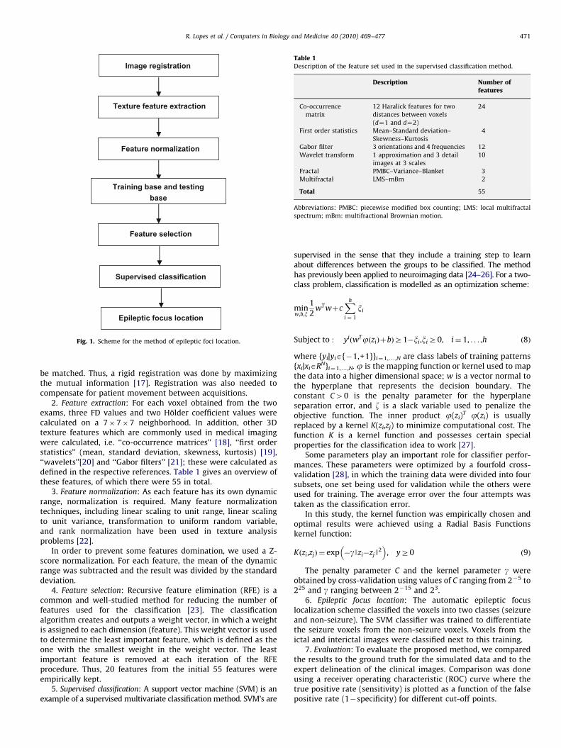
In this part, we detail the method used to localize the epilepticfocus. As depicted in Fig. 1, the method is composed of thefollowing steps:

1. Image registration: In order to be able to perform a voxel byvoxel comparison of ictal and interictal images, the images must

ARTICLE IN PRESS

Image registration

Texture feature extraction

Feature normalization

Training base and testing base

Feature selection

Supervised classification

Epileptic focus location

Fig. 1. Scheme for the method of epileptic foci location.

Table 1Description of the feature set used in the supervised classification method.

Description Number offeatures

Co-occurrence

matrix

12 Haralick features for two

distances between voxels

(d¼1 and d¼2)

24

First order statistics Mean–Standard deviation–

Skewness–Kurtosis

4

Gabor filter 3 orientations and 4 frequencies 12

Wavelet transform 1 approximation and 3 detail

images at 3 scales

10

Fractal PMBC–Variance–Blanket 3

Multifractal LMS–mBm 2

Total 55

Abbreviations: PMBC: piecewise modified box counting; LMS: local multifractal

spectrum; mBm: multifractional Brownian motion.

R. Lopes et al. / Computers in Biology and Medicine 40 (2010) 469–477 471

be matched. Thus, a rigid registration was done by maximizingthe mutual information [17]. Registration was also needed tocompensate for patient movement between acquisitions.

2. Feature extraction: For each voxel obtained from the twoexams, three FD values and two Holder coefficient values werecalculated on a 7�7�7 neighborhood. In addition, other 3Dtexture features which are commonly used in medical imagingwere calculated, i.e. ‘‘co-occurrence matrices’’ [18], ‘‘first orderstatistics’’ (mean, standard deviation, skewness, kurtosis) [19],‘‘wavelets’’[20] and ‘‘Gabor filters’’ [21]; these were calculated asdefined in the respective references. Table 1 gives an overview ofthese features, of which there were 55 in total.

3. Feature normalization: As each feature has its own dynamicrange, normalization is required. Many feature normalizationtechniques, including linear scaling to unit range, linear scalingto unit variance, transformation to uniform random variable,and rank normalization have been used in texture analysisproblems [22].

In order to prevent some features domination, we used a Z-score normalization. For each feature, the mean of the dynamicrange was subtracted and the result was divided by the standarddeviation.

4. Feature selection: Recursive feature elimination (RFE) is acommon and well-studied method for reducing the number offeatures used for the classification [23]. The classificationalgorithm creates and outputs a weight vector, in which a weightis assigned to each dimension (feature). This weight vector is usedto determine the least important feature, which is defined as theone with the smallest weight in the weight vector. The leastimportant feature is removed at each iteration of the RFEprocedure. Thus, 20 features from the initial 55 features wereempirically kept.

5. Supervised classification: A support vector machine (SVM) is anexample of a supervised multivariate classification method. SVM’s are

supervised in the sense that they include a training step to learnabout differences between the groups to be classified. The methodhas previously been applied to neuroimaging data [24–26]. For a two-class problem, classification is modelled as an optimization scheme:

minw,b,x

1

2wT wþc

Xh

i ¼ 1

xi

Subject to : yiðwTjðziÞþbÞZ1�xi,xiZ0, i¼ 1, . . . ,h ð8Þ

where {yi|yiA{�1,+1}}i¼1,y,N are class labels of training patterns{xi|xiARN}i¼1,y,N. j is the mapping function or kernel used to mapthe data into a higher dimensional space; w is a vector normal tothe hyperplane that represents the decision boundary. Theconstant C40 is the penalty parameter for the hyperplaneseparation error, and z is a slack variable used to penalize theobjective function. The inner product j(zi)

T j(zi) is usuallyreplaced by a kernel K(zi,zj) to minimize computational cost. Thefunction K is a kernel function and possesses certain specialproperties for the classification idea to work [27].

Some parameters play an important role for classifier perfor-mances. These parameters were optimized by a fourfold cross-validation [28], in which the training data were divided into foursubsets, one set being used for validation while the others wereused for training. The average error over the four attempts wastaken as the classification error.

In this study, the kernel function was empirically chosen andoptimal results were achieved using a Radial Basis Functionskernel function:

Kðzi,zjÞ ¼ exp �gJzi�zjJ2

� �, yZ0 ð9Þ

The penalty parameter C and the kernel parameter g wereobtained by cross-validation using values of C ranging from 2�5 to225 and g ranging between 2�15 and 23.

6. Epileptic focus location: The automatic epileptic focuslocalization scheme classified the voxels into two classes (seizureand non-seizure). The SVM classifier was trained to differentiatethe seizure voxels from the non-seizure voxels. Voxels from theictal and interictal images were classified next to this training.

7. Evaluation: To evaluate the proposed method, we comparedthe results to the ground truth for the simulated data and to theexpert delineation of the clinical images. Comparison was doneusing a receiver operating characteristic (ROC) curve where thetrue positive rate (sensitivity) is plotted as a function of the falsepositive rate (1�specificity) for different cut-off points.

ARTICLE IN PRESS


Sensitivity was calculated as

sensitivity¼true positive

true positiveþ false negativeð10Þ

and specificity as:

specificity¼true negative

true negativeþ false positiveð11Þ

We also used Youden’s index, estimated as

Youden’s index¼ specificityþsensitivity�1 ð12Þ

3. Validation on simulated IMAGES

3.1. Data

As there is no ground truth for real data, the developedalgorithm was first validated on simulated images. Using the MNISPECT template (www.mni.mcgill.ca), we simulated 1 interictaland 10 ictal scans with foci of known sizes and intensities, asdefined by [29]. This template corresponds to the mean of 22healthy subject scans obtained from the Department of NuclearMedicine of the Queen Elizabeth Hospital in Adelaide, Australia.These examinations were reconstructed as 91 transverse slices of91�109 isotropic voxels (2�2�2 mm3). Although this spatialresolution is higher than those obtained in clinical situations, thistemplate is frequently used for statistical parametric modelingand group studies on SPECT and PET images [30].

For the construction of the interictal image, the right anteriortemporal lobe was delineated and each voxel value in this areawas multiplied by 0.9 in order to model a 10% interictal decreaseof cerebral blood flow.

For the construction of the ictal images, all voxel values ofthe template were multiplied by 0.85 in order to model theradioactive decay between the filling of the syringe and theinjection time. A focus was then drawn inside the right temporallobe. Each focus voxel value was multiplied by a coefficient,yielding 10 different ictal scans corresponding to increased

Fig. 2. Quantification of the effectiveness of the classification in measuring the value of

mean AUC value of nine simulated images.

temporal blood flows, increasing in steps of +5%, from +5%to +50%.

Finally, random noise was added to the simulated data, inorder to provide more clinically realistic images. We multipliedeach voxel value by a number randomly chosen in the set [�13%;+13%]. This set was proposed by Boussion et al. [29] by applyingBudinger’s formula [31].

3.2. Quantitative results

One 3D ictal image was used for the training step. This imagecorresponded to the scan with an increased temporal blood flowof 20%. In order to perform a fourfold cross-validation of the SVM,the voxels set of this image was divided into four subsets. Thenine other images were used for the testing step.

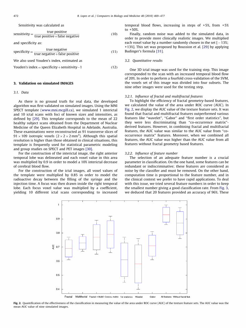
3.2.1. Influence of fractal and multifractal features

To highlight the efficiency of fractal geometry-based features,we calculated the value of the area under ROC curve (AUC). InFig. 2, we display the AUC value of the texture feature sets. It wasfound that fractal and multifractal features outperformed variousfeatures like ‘‘wavelet’’, ‘‘Gabor’’ and ‘‘first order statistics’’, butthey were less discriminating than ‘‘co-occurrence matrix’’-derived features. However, in combining fractal and multifractalfeatures, the AUC value was similar to the AUC value from ‘‘co-occurrence matrix’’ features. Moreover, when we combined allfeatures, the AUC value was higher than the AUC value from allfeatures without fractal geometry based features.

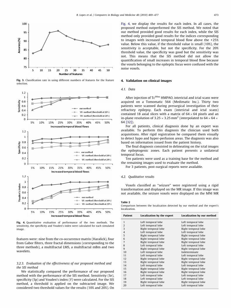
3.2.2. Influence of feature number

The selection of an adequate feature number is a crucialparameter in classification. On the one hand, some features can beredundant or indiscriminative; these features are considered asnoise by the classifier and must be removed. On the other hand,computation time is proportional to the feature number, and inthe clinical context we prefer to have rapid applications. To dealwith this issue, we tried several feature numbers in order to keepthe smallest number giving a good classification rate. From Fig. 3,we deduced that 20 features provided an accuracy of 96%. These

the area under ROC curve (AUC) of the texture feature sets. The AUC value was the

www.mni.mcgill.ca

www.mni.mcgill.ca

www.mni.mcgill.ca

www.mni.mcgill.ca

ARTICLE IN PRESS

Fig. 3. Classification rate in using different numbers of features for the feature

selection.

Fig. 4. Quantitative evaluation of performance of the two methods. The

sensitivity, the specificity and Youden’s index were calculated for each simulated

image.

Table 2Comparison between the localization detected by our method and the expert’s

localization.

Patient Localization by the expert Localization by our method

1 Left temporal lobe Left temporal lobe


3 Right temporal lobe Right temporal lobe







10 Left temporal lobe Indeterminate


features were: nine from the co-occurrence matrix (Haralick), fourfrom Gabor filters, three fractal dimensions (corresponding to thethree methods), a multifractal LMS, a multifractal mBm and twowavelets.











3.2.3. Evaluation of the effectiveness of our proposed method and

the SIS method

We statistically compared the performance of our proposedmethod with the performance of the SIS method. Sensitivity (Se),specificity (Sp) and Youden’s index (Y) were calculated. For the SISmethod, a threshold is applied on the subtracted image. Weconsidered two threshold values for the results (10% and 20%). On

Fig. 4, we display the results for each index. In all cases, theproposed method outperformed the SIS method. We noted thatour method provided good results for each index, while the SISmethod only provided good results for the indices correspondingto images with increased temporal blood flow above the +25%value. Below this value, if the threshold value is small (10%), thesensitivity is acceptable, but not the specificity. For the 20%threshold value, the specificity was good but the sensitivity wasnot. This means that the SIS method did not allow thequantification of small increases in temporal blood flow becausethe voxels belonging to the epileptic focus were confused with thenoise voxels.

4. Validation on clinical images

4.1. Data

After injection of Tc99m HMPAO, interictal and ictal scans wereacquired on a Tomomatic 564 (Medimatic Inc.). Thirty twopatients were scanned during presurgical investigation of theirrefractory epilepsy. Each exam (interictal and ictal scans)contained 18 axial slices with a matrix of 64�64 pixels and anin-plane resolution of 3.25�3.25 mm2 (interpolated to 64�64�64 [32]).

For all patients, clinical diagnosis done by an expert wasavailable. To perform this diagnosis the clinician used bothacquisitions. After rigid registration he compared them visuallyto detect hypo and hyper-perfusion areas. The diagnosis was alsobased on information issued from the patient history.

The final diagnosis consisted in delineating on the ictal imagesthe epileptogenic zones. Each patient presents a unilateraltemporal focus.

Ten patients were used as a training base for the method andthe remaining images used to evaluate the method.

For 3 patients, post-surgical reports were available.

4.2. Qualitative results

Voxels classified as ‘‘seizure’’ were registered using a rigidtransformation and displayed on the MR image. If this image wasnot available, the seizure voxels were displayed on the MNI MR

ARTICLE IN PRESS

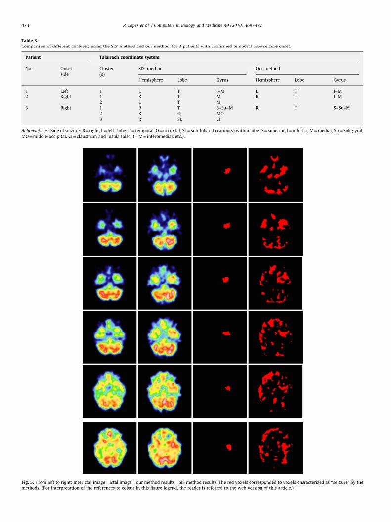
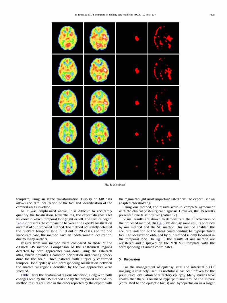
Fig. 5. From left to right: Interictal image—ictal image—our method results—SIS method results. The red voxels corresponded to voxels characterized as ‘‘seizure’’ by the

methods. (For interpretation of the references to colour in this figure legend, the reader is referred to the web version of this article.)

Table 3Comparison of different analyses, using the SIS’ method and our method, for 3 patients with confirmed temporal lobe seizure onset.

Patient Talairach coordinate system

No. Onset

side

Cluster

(s)

SIS’ method Our method

Hemisphere Lobe Gyrus Hemisphere Lobe Gyrus

1 Left 1 L T I–M L T I–M

2 Right 1 R T M R T I–M

2 L T M

3 Right 1 R T S–Su–M R T S–Su–M

2 R O MO

3 R SL CI

Abbreviations: Side of seizure: R¼right, L¼ left. Lobe: T¼temporal, O¼occipital, SL¼sub-lobar. Location(s) within lobe: S¼superior, I¼ inferior, M¼medial, Su¼Sub-gyral,

MO¼middle-occipital, CI¼claustrum and insula (also, I�M¼ inferomedial, etc.).


ARTICLE IN PRESS

Fig. 5. (Continued)


template, using an affine transformation. Display on MR dataallows accurate localization of the foci and identification of thecerebral areas involved.

As it was emphasized above, it is difficult to accuratelyquantify the localization. Nevertheless, the expert diagnosis letus know in which temporal lobe (right or left) the seizure began.Table 2 presents the comparison between the expert’s localizationand that of our proposed method. The method accurately detectedthe relevant temporal lobe in 19 out of 20 cases. For the oneinaccurate case, the method gave an indeterminate localization,due to many outliers.

Results from our method were compared to those of theclassical SIS method. Comparison of the anatomical regionsdetected by both approaches was done using the Talairachatlas, which provides a common orientation and scaling proce-dure for the brain. Three patients with surgically confirmedtemporal lobe epilepsy and corresponding localization betweenthe anatomical regions identified by the two approaches wereselected.

Table 3 lists the anatomical regions identified, along with bothchanges seen by the SIS method and by the proposed method. SISmethod results are listed in the order reported by the expert, with

the region thought most important listed first. The expert used anadapted thresholding.

Using our method, the results were in complete agreementwith the clinical post-surgical diagnosis. However, the SIS resultspresented one false positive (patient 2).

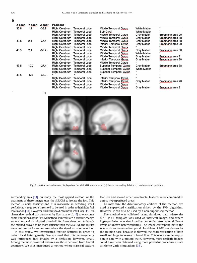
Visual results are shown to demonstrate the effectiveness ofthe proposed method. On Fig. 5, we display some results obtainedby our method and the SIS method. Our method enabled theaccurate isolation of the areas corresponding to hyperperfusedfoci. The localization obtained by our method is only localized inthe temporal lobe. On Fig. 6, the results of our method areregistered and displayed on the MNI MRI template with thecorresponding Talairach coordinates.

5. Discussion

For the management of epilepsy, ictal and interictal SPECTimaging is routinely used. Its usefulness has been proven for thepre-surgical evaluation of refractory epilepsy. Many studies haveshown that there is localized hyperperfusion around the seizure(correlated to the epileptic focus) and hypoperfusion in a larger

ARTICLE IN PRESS

Fig. 6. (a) Our method results displayed on the MNI MRI template and (b) the corresponding Talairach coordinates and positions.


surrounding area [33]. Currently, the most applied method for thetreatment of these images uses the SISCOM to isolate the foci. Thismethod is noise sensitive and it is inaccurate in detecting smallperfusions. It requires a threshold to be used in order to highlight focilocalization [34]. However, this threshold can mask small foci [35]. Analternative method was proposed by Rossman et al. [6] to overcomesome limitations of the SISOM method. It introduced a relative changesubtraction and an adapted threshold for focus detection. Althoughthe method proved to be more efficient than the SISCOM, the resultswere not precise for some cases where the signal variation was low.

In this study, we investigated texture features in order todetect local heterogeneity. We assumed that this heterogeneitywas introduced into images by a perfusion, however, small.Among the most powerful features are those deduced from fractalgeometry. We thus introduced a method where classical texture

features and second order local fractal features were combined todetect hyperperfused areas.

To maximize the discriminatory abilities of the method, weused a supervised classification driven by the SVM algorithm.However, it can also be used by a non-supervised method.

The method was validated using simulated data where theMNI SPECT template was used as interictal image, and wherehyperperfusion was simulated by randomly introducing differentlevels of known heterogeneities. The image corresponding to thescan with an increased temporal blood flow of 20% was chosen forthe training base, because it allowed the characterization of bothsmall and large increases in blood flow. This was a simple way toobtain data with a ground-truth. However, more realistic imagescould have been obtained using more powerful procedures, suchas Monte-Carlo simulations [36].

ARTICLE IN PRESS


By using these data, we proved the efficiency of these fractalfeatures for detecting small texture changes. Moreover, thesefeatures were more powerful than classical texture features.Another important result was that the effectiveness of the fractalfeatures improved when they were combined with other texturefeatures.

After this initial validation, the method was evaluated onclinical images of 22 patients diagnosed with refractory epilepsyin the temporal lobe. The results were compared to the referencemethod: SIS. It appeared that our method displayed increasedspecificity with good sensitivity. Moreover, the outlined temporalfoci were less voluminous than on the subtracted images obtainedwith the SIS method.

6. Conclusion

This study presents preliminary work; the next step will be thecharacterization of frontal lobe epileptic foci. For these kind ofpathologies, the interictal and ictal image subtraction which iscurrently used does not allow focus localization, because thecerebral blood flow variation is very small between the two scans.Moreover, frontal lobe foci are often smaller than temporal lobe foci,so they are often masked by the thresholding step in the SIS method.

As fractal geometry does not compare intensities betweeninterictal and ictal images voxels, but instead compares the localheterogeneity between these scans, it is less noise sensitive. Inaddition, as it does not make use of gray-level thresholding, ourmethod is less operator-dependent than other current methods.All these reasons, as illustrated by these promising results, lead usto expect an increased ability to detect small lesions in the future.

Conflict of interest statement

None declared.

References

[1] R. Duncan, J. Patterson, R. Roberts, et al., Ictal/postictal SPECT in the presurgicllocalisation of complex partial seizures, Journal of Neurology, Neurosurgery &Psychiatry 56 (1993) 141–148.

[2] C.C. Rowe, S.F. Berkovic, M.C. Austin, et al., Visual and quantitative analysis ofinterictal SPECT Tc99m HMPAO in temporal lobe epilepsy, Journal of NuclearMedicine 32 (1991) 1688–1694.

[3] M.D. Devous Sr., R.A. Thisted, G.F. Morgan, R.F. Leroy, C.C. Rowe, SPECT brainimaging in epilepsy: a meta-analysis, The Journal of Nuclear Medicine 39 (2)(1998) 285–293.

[4] M.O. Habert, G. Huberfeld, Ictal single photon computed tomography andSISCOM: methods and utility, Neurochirurgie 54 (3) (2008) 226–230.

[5] T.J. O’Brien, E.L. So, B.P. Mullan, M.F. Hauser, B.H. Brinkmann, N.I. Bohnen, D.Hanson, G.D. Cascino, C.R. Jack Jr., F.W. Sharbrough, Subtraction ictal SPECTco-registered to MRI improves clinical usefulness of SPECT in localizing thesurgical seizure focus, Neurology 50 (1998) 445–454.

[6] M. Rossman, M. Adjouadi, I. Yaylali, An interactive interface for seizure focuslocalization using SPECT image analysis, Computers in Medicine and Biology36 (1) (2006) 70–88.

[7] V. Bouilleret, M.P. Valenti, E. Hirsch, F. Semah, I.J. Namer, Correlation betweenPET and SISCOM in temporal lobe epilepsy, The Journal of Nuclear Medicine43 (8) (2002) 991–998.

[8] C. Chen, J. DaPonte, M. Fox, Fractal feature analysis and classification inmedical imaging, IEEE Transactions on Medical Imaging 8 (2) (1989) 133–142.

[9] D. Chen, R. Chang, C. Chen, M. Ho, S. Kuo, S. Hung, W. Moon, Classification ofbreast ultrasound images using fractal feature, Clinical Imaging 29 (4) (2005)235–245.

[10] S. Mallat, W.H. Whang, Singularity detection and processing with wavelets,IEEE Transaction on Information Theory 38 (1992) 617–643.

[11] J. Zook, K. Iftekharuddin, Statistical analysis of fractal-based brain tumordetection algorithms, Magnetic Resonance Imaging 23 (2005) 671–678.

[12] K. Iftekharuddin, C. Parra, Multiresolution-fractal feature extraction andtumor detection: analytical model and implementation, in: Proceedings ofSPIE Wavelets: Applications in Signal and Image Processing X, vol. 5207,2003.

[13] A. Islam, K. Iftekharuddin, R. Ogg, F. Laningham, B. Sivakumar, Multifractalmodeling, segmentation, prediction and statistical validation of posteriorfossa tumors, in: Proceedings of SPIE Medical Imaging: Computer-aideddiagnosis, vol. 6915, 2008, pp. 1–11.

[14] S. Novianto, Y. Suzuki, J. Maeda, Near optimum estimation of local fractaldimension for image segmentation, Pattern Recognition Letters 24 (1–3)(2003) 365–374.

[15] B. Mandelbrot, J. Van Ness, Fractional Brownian motion, fractional noises andapplications, S.I.A.M. Review 10 (1968) 422–437.

[16] R. Lopes, P. Dubois, N. Makni, W. Szurhaj, S. Maoucje, N. Betrouni,Classification of brain SPECT imaging using 3D local multifractal spectrumfor epilepsy detection, International Journal of Computer Assisted Radiologyand Surgery 3 (4–5) (2008) 341–346.

[17] F. Maes, A. Collignon, D. Vandermeulen, G. Marchal, P. Suetens, Multimodalityimage registration by maximiation of mutual information, in: MathematicalMethods in Biomedical Image Analysis, IEEE Computer Society Press, LosAlamitos, CA, 1996, pp. 14–22.

[18] W. Chen, M.L. Giger, H. Li, U. Bick, G.M. Newstead, Volumetric textureanalysis of breast lesions on contrast-enhanced magnetic resonance images,Magnetic Resonance in Medicine 58 (2007) 562–571.

[19] V. Kovalev, F. Kruggel, H. Gertz, D. Cramon, Three-dimensional textureanalysis of MRI brain datasets, IEEE Transactions on Medical Imaging 20 (5)(2001) 424–433.

[20] K. Jafari-Khousani, H. Soltanian-Zadeh, K. Elisevich, S. Patel, Comparison of 2Dand 3D wavelet features for the characterization, in: Proceedings of SPIEMedical Imaging: Physiology, Function and Structure from Medical Images,vol. 5369, 2004. pp. 593–601.

[21] A. Madabhushi, M. Feldman, D. Metaxas, J. Tomaszeweski, D. Chute,Automated detection of prostatic adenocarcinoma from high-resolutionex vivo MRI, IEEE Transactions on Medical Imaging 24 (12) (2005) 1611–1625.

[22] S. Aksoy, R. Haralick, Feature normalization and likelihood-based similaritymeasures for image retrieval, Pattern Recognition Letters 22 (5) (2001)563–582.

[23] M.D. Shieh, C.C. Yang, Multiclass SVM-RFE for product from feature selection,Expert Systems with Applications 35 (1–2) (2008) 531–541.

[24] Y. Kawasaki, M. Suzuki, F. Kherif, T. Takahashi, S.Y. Zhou, K. Nakamura, M.Matsui, T. Sumiyoshi, H. Seto, M. Kurachi, Multivariate voxel-basedmorphometry successfully differentiates schizophrenia patients from healthycontrols, NeuroImage 34 (2007) 235–242.

[25] Z. Lao, D. Shen, Z. Xue, B. Karacali, S.M. Resnick, C. Davatzikos, Morphologicalclassification of brains via high-dimensional shape transformations andmachine learning methods, NeuroImage 21 (2004) 46–57.

[26] J. Mourao-Miranda, A.L.W. Bokde, C. Born, H. Hampel, M. Stetter, Classifyingbrain states and determining the discriminating activation patterns:support vector machine on functional MRI data, NeuroImage 28 (2005)980–995.

[27] N. Cristianini, J. Shawe-taylor, An Introduction to Support Vector Machinesand other Kernel-Based Learning Methods, Cambridge Univeristy Press,United Kingdom, 2000.

[28] R. Duda, P. Hart, D. Stork, Pattern Classification, Wiley, New-York, 2001.[29] N. Boussion, C. Houzard, K. Ostrowsky, P. Ryvlin, F. Maugui �ere, L. Cinotti,

Automated detection of local normalization areas for icatl–interictalsubtraction brain SPECT, Journal of Nuclear Medicine 43 (2002) 1419–1425.

[30] E.A. Stamatakis, J.T.L. Wilson, D.J. Wyper, Spatial normalization of lesionedHMPAO-SPECT Images, NeuroImage 14 (4) (2001) 844–852.

[31] T.F. Budinger, Physical attributes of single-photon tomography, Journal ofNuclear Medicine 21 (1980) 579–592.

[32] P. Thevenaz, T. Blu, M. Unser, Image interpolation and resampling, in:Bankman (Ed.), Hand book of Image Processing, 2000, pp. 393–420.

[33] C.C. Rowe, S.F. Berkovic, W.J. Mc Kay, P.F. Bladin, Patterns of postictal cerebralblood flow in temporal lobe epilepsy: qualitative and quantitative analysis,Neurology 41 (7) (1991) 1096–1103.

[34] W. Van Paesschen, Ictal SPECT, Epilepsia 45 (4) (2004) 35–40.[35] A. Kaminska, C. Chiron, D. Ville, G. Dellatolas, A. Hollo, C. Cieuta, C. Jalin, O.

Delalande, M. Fhlen, P. Vera, C. Soufflet, O. Dulac, Ictal SPECT in children withepilepsy: comparison with intracranial EEG and relation to postsurgicaloutcome, Brain 126 (2003) 248–260.

[36] K. Assie, V. Breton, I. Buvat, C. Comtat, S. Jan, M. Krieguer, D. Lazaro, C. Morel,M. Rey, G. Santin, L. Simon, S. Staelens, D. Strul, J.M. Vieira, R. Van deWalle, Monte Carlo simulation in PET and SPECT instrumentation usingGATE, Nuclear Instruments and Methods in Physics Research A 527 (2004)180–189.

Documents

Fractal features for localization of temporal lobe epileptic foci using SPECT imaging