Grid generation using lemniscates with two foci

Mathematical and Computer Modelling ( ) –

Contents lists available at ScienceDirect

Mathematical and Computer Modelling

journal homepage: www.elsevier.com/locate/mcm

Grid generation using lemniscates with two fociM. Lentini a,∗, L. Cardona b, M. Paluszny a

a Universidad Nacional de Colombia, Colombiab Jovenes investigadores, Colciencias, Colombia

a r t i c l e i n f o

Article history:Received 26 October 2010Received in revised form 2 May 2011Accepted 3 May 2011

Keywords:LemniscatesOrthogonal gridPath approximationNonlinear least squares

a b s t r a c t

We consider the approximation of planar curves by pairs of two-foci lemniscates that arestitched together continuously. Lemniscates are level curves of the absolute value of anunivariate complex polynomial. We want to build orthogonal grids on offshore areas, andon elongated regionswith changingwidth using lemniscateswith two foci. Such grids havemany advantages in the numerical modeling of problems such as contaminant transport inrivers and also in areas of 3D visualization such as terrain modeling. The main applicationis in the areas of numerical solution of PDEs and computer aided geometric design. Wereport on the results of numerical experiments performed with MATLAB R⃝using data fromthe San Andrés island and the Guajira peninsula in Colombia and the Orinoco river. In thispaper we compare the exact distance between a point and a lemniscate with the estimatethat we have used in this paper and previous work.

© 2011 Elsevier Ltd. All rights reserved.

1. Introduction

The construction of grids on irregular regions has been an important topic in the development of software for numericallysolving partial differential equations. The discretization, via finite differences say, of a set of partial differential equationson a 2D region Ω requires a grid defined on the boundary and the interior of Ω where the properties of the phenomenonto be studied will be measured. In the literature, the most popular numerical procedures for generating a mesh on Ω are:conformal mapping methods, elliptic grid generation and the variational methods. More recently the use of lemniscatesto construct orthogonal grids has been presented as a competitive alternative. Grid orthogonality is a desirable propertyfor the convergence and stability of the numerical algorithms. Useful reviews of orthogonal and nearly orthogonal gridson 2D regions include [1,2] and the references therein. In [2] it is stated that the problem of generating an orthogonal gridon an irregular region is not fully settled yet. A method based on lemniscates of complex polynomials of degree 3 waspresented in [3,4] as an alternative for meander like regions. There it was proposed to ‘‘tile’’ the region with lemniscaticsectors. A lemniscatic sector is the area bounded by two confocal lemniscates and two arcs; the latter are orthogonal tothe lemniscates. The two continuous curves given by joining corresponding lemniscatic segments of contiguous lemniscaticsectors approximate the boundary of the region. Any two neighboring lemniscatic sectors meet, within a given tolerance,along a common arc. The method relies on the solution of a nonlinear least squares problem.

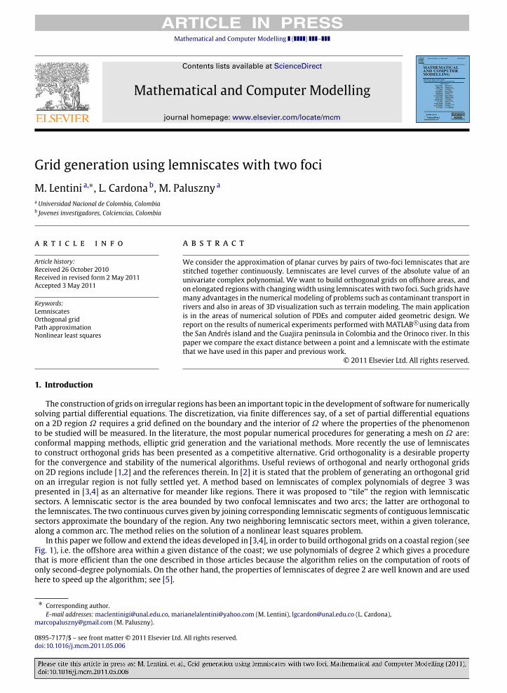
In this paper we follow and extend the ideas developed in [3,4], in order to build orthogonal grids on a coastal region (seeFig. 1), i.e. the offshore area within a given distance of the coast; we use polynomials of degree 2 which gives a procedurethat is more efficient than the one described in those articles because the algorithm relies on the computation of roots ofonly second-degree polynomials. On the other hand, the properties of lemniscates of degree 2 are well known and are usedhere to speed up the algorithm; see [5].

∗ Corresponding author.E-mail addresses:[email protected], [email protected] (M. Lentini), [email protected] (L. Cardona),

[email protected] (M. Paluszny).

0895-7177/$ – see front matter© 2011 Elsevier Ltd. All rights reserved.doi:10.1016/j.mcm.2011.05.006

http://dx.doi.org/10.1016/j.mcm.2011.05.006

http://www.elsevier.com/locate/mcm

http://www.elsevier.com/locate/mcm

mailto:[email protected]




http://dx.doi.org/10.1016/j.mcm.2011.05.006

2 M. Lentini et al. / Mathematical and Computer Modelling ( ) –

Fig. 1. Satellite picture of the San Andrés island in Colombia.

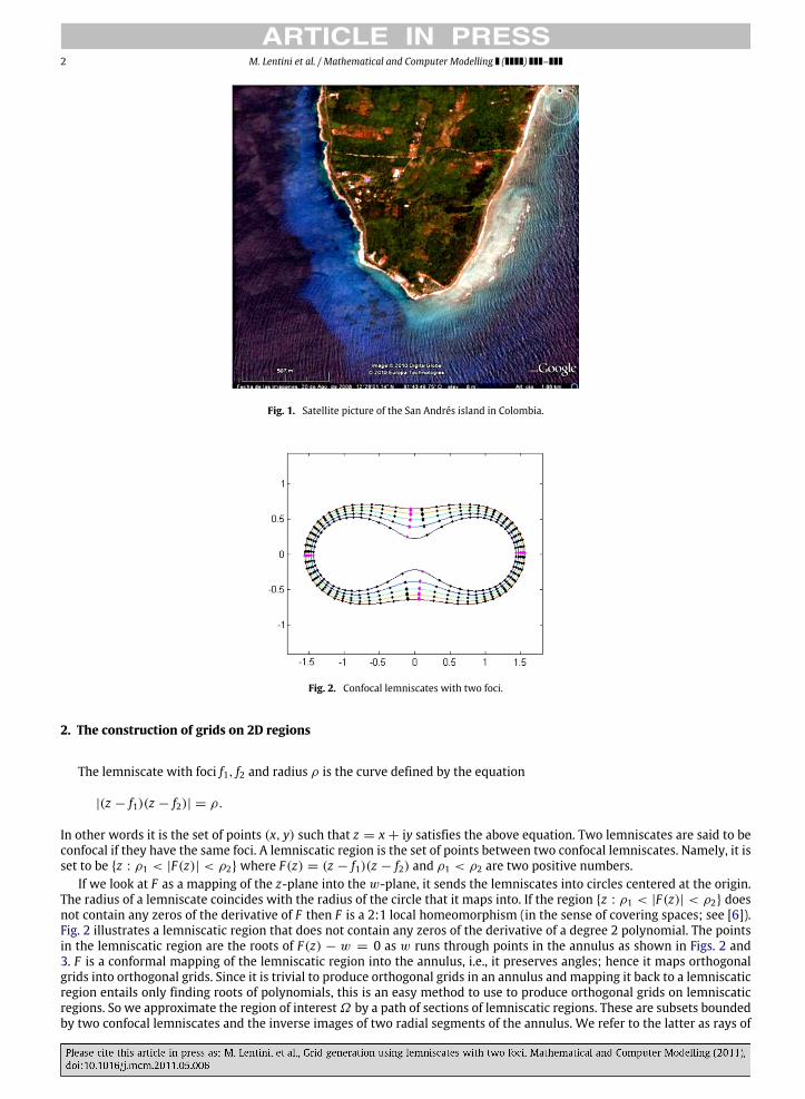
Fig. 2. Confocal lemniscates with two foci.

2. The construction of grids on 2D regions

The lemniscate with foci f1, f2 and radius ρ is the curve defined by the equation

|(z − f1)(z − f2)| = ρ.

In other words it is the set of points (x, y) such that z = x + iy satisfies the above equation. Two lemniscates are said to beconfocal if they have the same foci. A lemniscatic region is the set of points between two confocal lemniscates. Namely, it isset to be z : ρ1 < |F(z)| < ρ2 where F(z) = (z − f1)(z − f2) and ρ1 < ρ2 are two positive numbers.

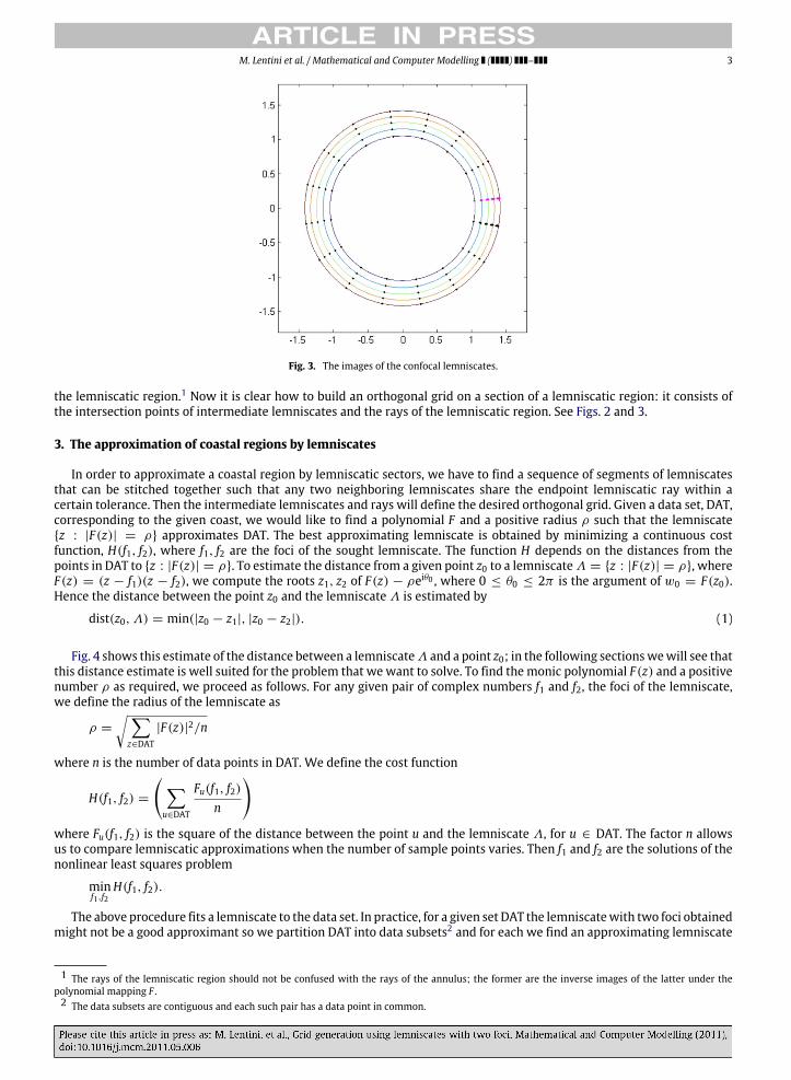
If we look at F as a mapping of the z-plane into the w-plane, it sends the lemniscates into circles centered at the origin.The radius of a lemniscate coincides with the radius of the circle that it maps into. If the region z : ρ1 < |F(z)| < ρ2 doesnot contain any zeros of the derivative of F then F is a 2:1 local homeomorphism (in the sense of covering spaces; see [6]).Fig. 2 illustrates a lemniscatic region that does not contain any zeros of the derivative of a degree 2 polynomial. The pointsin the lemniscatic region are the roots of F(z) − w = 0 as w runs through points in the annulus as shown in Figs. 2 and3. F is a conformal mapping of the lemniscatic region into the annulus, i.e., it preserves angles; hence it maps orthogonalgrids into orthogonal grids. Since it is trivial to produce orthogonal grids in an annulus and mapping it back to a lemniscaticregion entails only finding roots of polynomials, this is an easy method to use to produce orthogonal grids on lemniscaticregions. So we approximate the region of interest Ω by a path of sections of lemniscatic regions. These are subsets boundedby two confocal lemniscates and the inverse images of two radial segments of the annulus. We refer to the latter as rays of

M. Lentini et al. / Mathematical and Computer Modelling ( ) – 3

Fig. 3. The images of the confocal lemniscates.

the lemniscatic region.1 Now it is clear how to build an orthogonal grid on a section of a lemniscatic region: it consists ofthe intersection points of intermediate lemniscates and the rays of the lemniscatic region. See Figs. 2 and 3.

3. The approximation of coastal regions by lemniscates

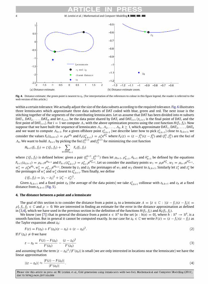
In order to approximate a coastal region by lemniscatic sectors, we have to find a sequence of segments of lemniscatesthat can be stitched together such that any two neighboring lemniscates share the endpoint lemniscatic ray within acertain tolerance. Then the intermediate lemniscates and rays will define the desired orthogonal grid. Given a data set, DAT,corresponding to the given coast, we would like to find a polynomial F and a positive radius ρ such that the lemniscatez : |F(z)| = ρ approximates DAT. The best approximating lemniscate is obtained by minimizing a continuous costfunction, H(f1, f2), where f1, f2 are the foci of the sought lemniscate. The function H depends on the distances from thepoints in DAT to z : |F(z)| = ρ. To estimate the distance from a given point z0 to a lemniscateΛ = z : |F(z)| = ρ, whereF(z) = (z − f1)(z − f2), we compute the roots z1, z2 of F(z) − ρeiθ0 , where 0 ≤ θ0 ≤ 2π is the argument of w0 = F(z0).Hence the distance between the point z0 and the lemniscate Λ is estimated by

dist(z0, Λ) = min(|z0 − z1|, |z0 − z2|). (1)

Fig. 4 shows this estimate of the distance between a lemniscateΛ and a point z0; in the following sectionswewill see thatthis distance estimate is well suited for the problem that we want to solve. To find themonic polynomial F(z) and a positivenumber ρ as required, we proceed as follows. For any given pair of complex numbers f1 and f2, the foci of the lemniscate,we define the radius of the lemniscate as

ρ =

z∈DAT

|F(z)|2/n

where n is the number of data points in DAT. We define the cost function

H(f1, f2) =

u∈DAT

Fu(f1, f2)n

where Fu(f1, f2) is the square of the distance between the point u and the lemniscate Λ, for u ∈ DAT. The factor n allowsus to compare lemniscatic approximations when the number of sample points varies. Then f1 and f2 are the solutions of thenonlinear least squares problem

minf1,f2

H(f1, f2).

The above procedure fits a lemniscate to the data set. In practice, for a given set DAT the lemniscatewith two foci obtainedmight not be a good approximant so we partition DAT into data subsets2 and for each we find an approximating lemniscate

1 The rays of the lemniscatic region should not be confused with the rays of the annulus; the former are the inverse images of the latter under thepolynomial mapping F .2 The data subsets are contiguous and each such pair has a data point in common.


1

0.5

0

-0.5

-1

-1.5

-2

-2.510.50-0.5-1 1.5-1.5 2-2

(a) Distance estimate. (b) Distance estimate zoom.

Fig. 4. Distance estimate; the green point is nearest to z0 . (For interpretation of the references to colour in this figure legend, the reader is referred to theweb version of this article.)

within a certain tolerance.We actually adjust the size of the data subsets according to the required tolerance. Fig. 6 illustratesthree lemniscates which approximate three data subsets of DAT coded with blue, green and red. The next issue is thestitching together of the segments of the contributing lemniscates. Let us assume that DAT has been divided intom subsetsDAT1,DAT2, . . . ,DATm and let zi,i+1 be the data point shared by DATi and DATi+1 (zi,i+1 is the final point of DATi and thefirst point of DATi+1). For i = 1 we compute Λ1 with the above optimization process using the cost function H(f1, f2). Nowsuppose that we have built the sequence of lemniscates Λ1, Λ2, . . . , Λk, k ≥ 1, which approximate DAT1,DAT2, . . . ,DATkand we want to compute Λk+1. For a given offshore point z∗

k,k+1 (we describe later how to pick z∗

k,k+1) close to zk,k+1, weconsider the values Fk(zk,k+1) = ρkeiθk and Fk(z∗

k,k+1) = ρ∗

k eiθ∗k where Fk(z) = (z − f k1 )(z − f k2 ) and (f k1 , f k2 ) are the foci of

Λk. We want to build Λk+1 by picking the foci f k+11 and f k+1

2 for minimizing the cost function

Hk+1(f1, f2) = ζ (f1, f2) +

u∈DATk+1

Fu(f1, f2)

where ζ (f1, f2) is defined below: given a pair (f k+11 , f k+1

2 ) then let ρk+1, ρ∗

k+1, θk+1 and θ∗

k+1 be defined by the equationsFk+1(zk,k+1) = ρk+1eiθk+1 and Fk+1(z∗

k,k+1) = ρ∗

k+1eiθ∗k+1 . Let us consider the auxiliary points w1 = ρkeiθ

∗k , w2 = ρk+1eiθ

∗k+1 ,

w∗

1 = ρ∗

k eiθk , w∗

2 = ρ∗

k+1eiθk+1 . Denote by z1 and z2 the preimages of w1 and w2 closest to zk,k+1. Similarly let z∗

1 and z∗

2 bethe preimages of w∗

1 and w∗

2 closest to z∗

k,k+1. Then finally, we define

ζ (f1, f2) = |z1 − z2|2 + |z∗

1 − z∗

2 |2.

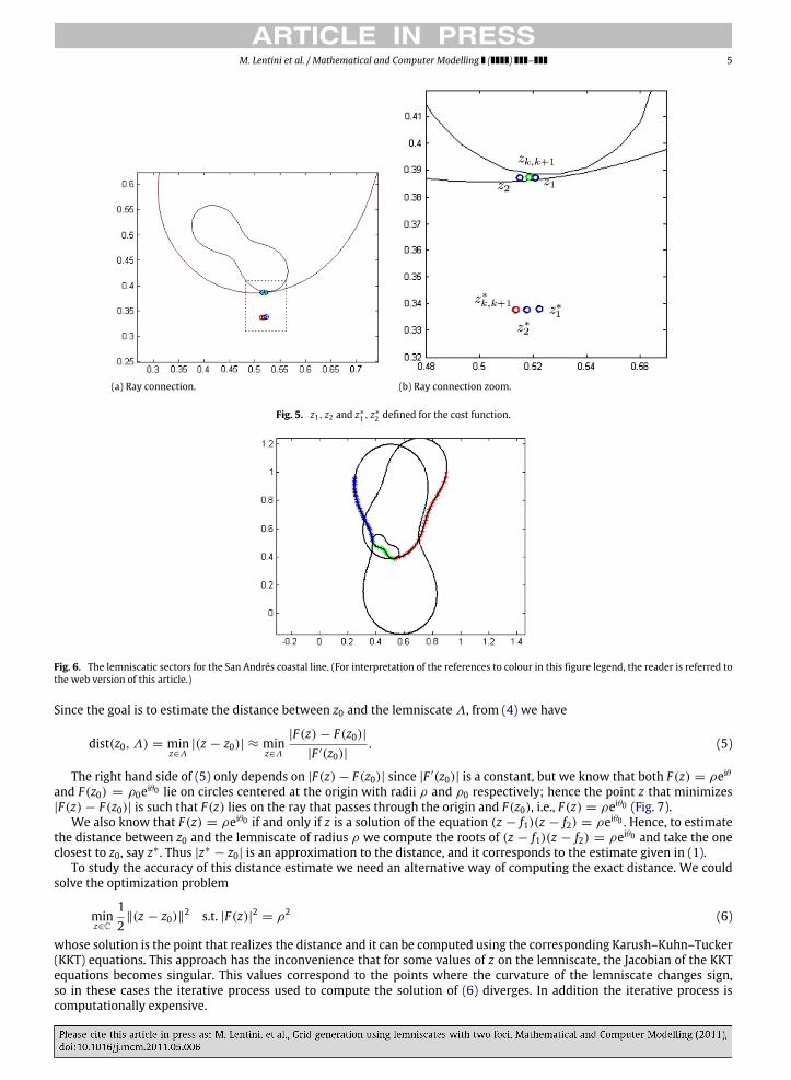
Given zk,k+1 and a fixed point zA (the average of the data points) we take z∗

k,k+1 collinear with zk,k+1 and zA at a fixeddistance from zk,k+1 (Fig. 5).

4. The distance between a point and a lemniscate

The goal of this section is to consider the distance from a point z0 to a lemniscate Λ = z ∈ C : |(z − f1)(z − f2)| =

ρ, f1, f2 ∈ C and ρ > 0. We are interested in finding an estimate for the error in the distance approximation as definedin [3,4], which we have used in the previous section in the definition of the functions H(f1, f2) and Hk(f1, f2).

We know (see [7]) that in general the distance from a point x ∈ Rn to the set x : h(x) = 0, where h : Rn→ Rk, is a

smooth function. But in general it cannot be computed exactly. In our case for z0 ∈ C we write F(z) = (z − f1)(z − f2) asthe Taylor expansion about z0:

F(z) = F(z0) + F ′(z0)(z − z0) + (z − z0)2. (2)If F ′(z0) = 0 we have

z − z0 =F(z) − F(z0)

F ′(z0)−

(z − z0)2

F ′(z0)(3)

and assuming that the term |z − z0|2/|F ′(z0)| is small (we are only interested in locations near the lemniscate) we have thelinear approximation

|(z − z0)| ≈|F(z) − F(z0)|

|F ′(z0)|. (4)


(a) Ray connection. (b) Ray connection zoom.

Fig. 5. z1, z2 and z∗

1 , z∗

2 defined for the cost function.

Fig. 6. The lemniscatic sectors for the San Andrés coastal line. (For interpretation of the references to colour in this figure legend, the reader is referred tothe web version of this article.)

Since the goal is to estimate the distance between z0 and the lemniscate Λ, from (4) we have

dist(z0, Λ) = minz∈Λ

|(z − z0)| ≈ minz∈Λ

|F(z) − F(z0)||F ′(z0)|

. (5)

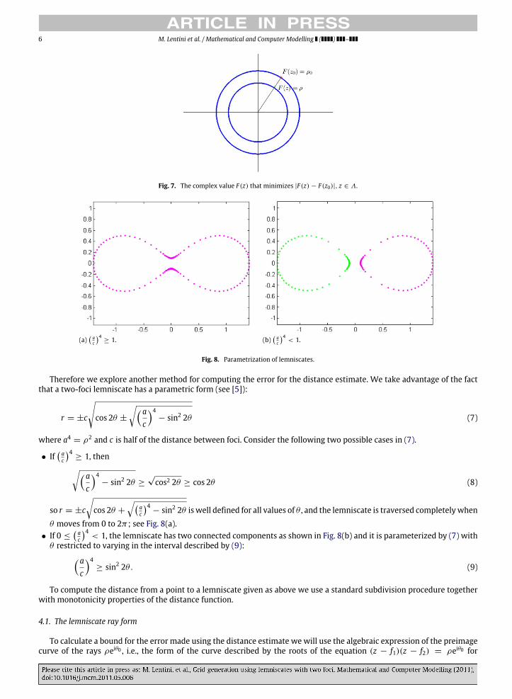
The right hand side of (5) only depends on |F(z) − F(z0)| since |F ′(z0)| is a constant, but we know that both F(z) = ρeiθand F(z0) = ρ0eiθ0 lie on circles centered at the origin with radii ρ and ρ0 respectively; hence the point z that minimizes|F(z) − F(z0)| is such that F(z) lies on the ray that passes through the origin and F(z0), i.e., F(z) = ρeiθ0 (Fig. 7).

We also know that F(z) = ρeiθ0 if and only if z is a solution of the equation (z − f1)(z − f2) = ρeiθ0 . Hence, to estimatethe distance between z0 and the lemniscate of radius ρ we compute the roots of (z − f1)(z − f2) = ρeiθ0 and take the oneclosest to z0, say z∗. Thus |z∗

− z0| is an approximation to the distance, and it corresponds to the estimate given in (1).To study the accuracy of this distance estimate we need an alternative way of computing the exact distance. We could

solve the optimization problem

minz∈C

12∥(z − z0)∥2 s.t. |F(z)|2 = ρ2 (6)

whose solution is the point that realizes the distance and it can be computed using the corresponding Karush–Kuhn–Tucker(KKT) equations. This approach has the inconvenience that for some values of z on the lemniscate, the Jacobian of the KKTequations becomes singular. This values correspond to the points where the curvature of the lemniscate changes sign,so in these cases the iterative process used to compute the solution of (6) diverges. In addition the iterative process iscomputationally expensive.


Fig. 7. The complex value F(z) that minimizes |F(z) − F(z0)|, z ∈ Λ.

(a) ac

4≥ 1. (b)

ac

4< 1.

Fig. 8. Parametrization of lemniscates.

Therefore we explore another method for computing the error for the distance estimate. We take advantage of the factthat a two-foci lemniscate has a parametric form (see [5]):

r = ±c

cos 2θ ±

ac

4− sin2 2θ (7)

where a4 = ρ2 and c is half of the distance between foci. Consider the following two possible cases in (7).

• If ac

4≥ 1, thena

c

4− sin2 2θ ≥

√

cos2 2θ ≥ cos 2θ (8)

so r = ±c

cos 2θ +

ac

4− sin2 2θ is well defined for all values of θ , and the lemniscate is traversed completelywhen

θ moves from 0 to 2π ; see Fig. 8(a).• If 0 ≤

ac

4< 1, the lemniscate has two connected components as shown in Fig. 8(b) and it is parameterized by (7) with

θ restricted to varying in the interval described by (9):ac

4≥ sin2 2θ. (9)

To compute the distance from a point to a lemniscate given as above we use a standard subdivision procedure togetherwith monotonicity properties of the distance function.

4.1. The lemniscate ray form

To calculate a bound for the error made using the distance estimate we will use the algebraic expression of the preimagecurve of the rays ρeiθ0 , i.e., the form of the curve described by the roots of the equation (z − f1)(z − f2) = ρeiθ0 for


(a) Absolute error ϵ, ρ = 0.9. (b) Absolute error ϵ, ρ = 1.1.

(c) Absolute error ϵ, ρ = 1.3. (d) Absolute error ϵ, ρ = 1.5.

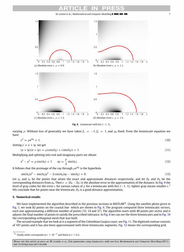
Fig. 9. Lemniscate with foci −1, 1.

varying ρ. Without loss of generality we have taken f1 = −1, f2 = 1, and ρ0 fixed. From the lemniscate equation wehave

z2 = ρeiθ0 + 1. (10)

Setting z = x + iy, we get

(x + iy)(x + iy) = ρ(cos(θ0) + i sin(θ0)) + 1. (11)

Multiplying and splitting into real and imaginary parts we obtain

x2 − y2 = ρ cos(θ0) + 1 xy =ρ

2sin(θ0). (12)

It follows that the preimage of the ray through ρeiθ0 is the hyperbola

sin(θ0)x2 − sin(θ0)y2 − 2 cos(θ0)xy − sin(θ0) = 0. (13)

Let zE and zA be the points that attain the exact and approximate distances respectively, and let DE and DA be thecorresponding distances from z0. Then ϵ = |DA −DE | is the absolute error in the approximation of the distance. In Fig. 9 thelevel of gray codes for the error ϵ for various values of ρ for a lemniscate with foci −1, 1; lighter gray means smaller ϵ.3We conclude that for points near the lemniscate, DA is a good distance approximation.

5. Numerical results

We have implemented the algorithm described in the previous sections in MATLAB R⃝. Using the satellite photo given inFig. 1, we took 82 points on the coastal line which are shown in Fig. 6. The program computed three lemniscatic sectors,each one approximating a different number of points (33, 14 and 37). The algorithm starts with 40 points per sector and itadjusts the final number of points to satisfy the prescribed tolerance. In Fig. 6 we can see the three lemniscates and in Fig. 10the corresponding orthogonal mesh that was built.

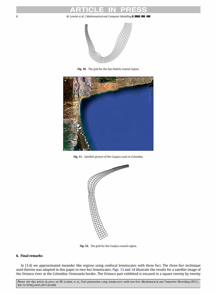
The second example thatwe look at is a segment of the ColombianGuajira coast; see Fig. 11. The digitized contour consistsof 107 points and it has also been approximated with three lemniscatic segments. Fig. 12 shows the corresponding grid.

3 Totally white corresponds to ϵ ≈ 10−17 and black to ϵ ≈ 0.2.


Fig. 10. The grid for the San Andrés coastal region.

Fig. 11. Satellite picture of the Guajira coast in Colombia.

Fig. 12. The grid for the Guajira coastal region.

6. Final remarks

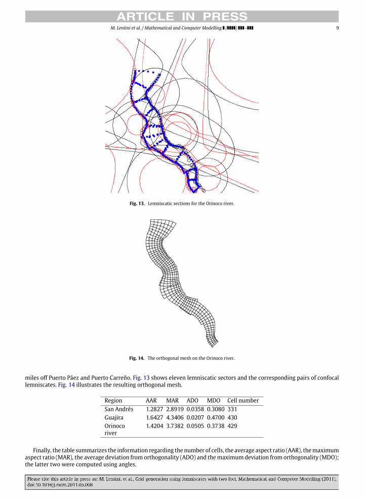
In [3,4] we approximated meander like regions using confocal lemniscates with three foci. The three-foci techniqueused therein was adapted in this paper to two-foci lemniscates. Figs. 13 and 14 illustrate the results for a satellite image ofthe Orinoco river at the Colombia–Venezuela border. The Orinoco part exhibited is encased in a square twenty by twenty


Fig. 13. Lemniscatic sections for the Orinoco river.

Fig. 14. The orthogonal mesh on the Orinoco river.

miles off Puerto Páez and Puerto Carreño. Fig. 13 shows eleven lemniscatic sectors and the corresponding pairs of confocallemniscates. Fig. 14 illustrates the resulting orthogonal mesh.

Region AAR MAR ADO MDO Cell numberSan Andrés 1.2827 2.8919 0.0358 0.3080 331Guajira 1.6427 4.3406 0.0207 0.4700 430Orinocoriver

1.4204 3.7382 0.0505 0.3738 429

Finally, the table summarizes the information regarding the number of cells, the average aspect ratio (AAR), themaximumaspect ratio (MAR), the average deviation from orthogonality (ADO) and themaximumdeviation from orthogonality (MDO);the latter two were computed using angles.


Acknowledgments

The authors thank the anonymous referees for their thoughtful comments which led to improvement of the paper. Theauthors also thank Colciencias, Programa de Jóvenes Investigadores e Innovadores, and Universidad Nacional de Colombia,Sede Medellín, for financial support for this work.

References

[1] V. Akcelik, B. Jaramaz, O. Ghattas, Nearly orthogonal two dimensional grid generation with aspect ratio control, Journal of Computational Physics 171(2001) 805–821.

[2] P. Barrera Sanchez, G.F. Gonzalez Flores, F.J. Dominguez Mota, Some experiences on orthogonal grid generation, Applied Numerical Mathematics 40(2002) 179–190.

[3] M. Lentini, M. Paluszny, Approximation of meander-like regions by paths of lemniscatic sectors and the computation of orthogonal meshes, ComputerAided Geometric Design 25 (9) (2008) 729–737.

[4] M. Lentini, M. Paluszny, Orthogonal grids on meander-like regions, Electronic Transactions on Numerical Analysis 34 (2008) 1–13.[5] A.E. Hirst, E.K. Lloyd, Cassini, his ovals and a space probe to Saturn, The Mathematical Gazette 81 (492) (1997) 409–421.[6] J.R. Munkres, Topology, second ed., Prentice Hall, 1999.[7] G. Taubin, Estimation of planar curves, surfaces, and nonplanar space curves defined by implicit equations with applications to edge and range image

segmentation, IEEE Transactions on Pattern Analysis and Machine Intelligence 13 (11) (1991) 1115–1138.

Documents

Grid generation using lemniscates with two foci