Available online at www.sciencedirect.com

Data & Knowledge Engineering 64 (2008) 266–293

www.elsevier.com/locate/datak

Fragment-based approximate retrieval in highlyheterogeneous XML collections

I. Sanz a, M. Mesiti b,*, G. Guerrini c, R. Berlanga a

a Department of Computer Science and Engineering, Universitat Jaume I, Avg. de Vicent Sos Baynat, s/n E-12071 Castello, Spainb Dipartimento di Informatica e Comunicazione, Universita degli Studi di Milano, Via Comelico, 39/41 I-20135 Milano, Italy

c Dipartimento di Informatica e Scienze dell’Informazione, Universita degli Studi di Genova, Via Dodecaneso, 35 I-16146 Genova, Italy

Received 30 January 2007; accepted 24 May 2007Available online 6 August 2007

Abstract

Due to the heterogeneous nature of XML data for internet applications exact matching of queries is often inadequate.The need arises to quickly identify subtrees of XML documents in a collection that are similar to a given pattern. Similarityinvolves both tags, that are not required to coincide, and structure, in which not all the relationships among nodes in thetree structure are strictly preserved.

In this paper we present an efficient approach to the identification of similar subtrees, relying on ad-hoc indexing struc-tures. The approach allows to quickly detect, in a heterogeneous document collection, the minimal portions that exhibitsome similarity with the pattern. These candidate portions are then ranked according to their actual similarity. Theapproach supports different notions of similarity, thus it can be customized to different application domains. In the paper,three different similarity measures are proposed and compared. The approach is experimentally validated and the exper-imental results are extensively discussed.� 2007 Elsevier B.V. All rights reserved.

Keywords: XML; Approximate structural retrieval; Enhanced indexing techniques

1. Introduction

Interoperability among systems is commonly achieved through the interchange of XML documents thatcan represent a great variety of information resources: semi-structured data, database schemas, concepttaxonomies, ontologies, etc. Most XML document collections are highly heterogeneous from severalviewpoints. The first level of heterogeneity is tag heterogeneity: vocabulary discrepancies may occur in the ele-ment tags. Two elements representing the same information can be labelled by tags that are stems (e.g.,author and authors), that are one substring of the other (e.g., authors and co-authors), or that

0169-023X/$ - see front matter � 2007 Elsevier B.V. All rights reserved.

doi:10.1016/j.datak.2007.05.008

* Corresponding author.E-mail addresses: Ismael.Sanz@uji.es (I. Sanz), mesiti@dico.unimi.it (M. Mesiti), guerrini@disi.unige.it (G. Guerrini), berlanga@uji.es

(R. Berlanga).

I. Sanz et al. / Data & Knowledge Engineering 64 (2008) 266–293 267

are similar according to a given thesaurus (e.g., author and writer). The second level of heterogeneity isstructural heterogeneity that results in documents with different hierarchical structures. Structural heterogene-ity can be produced by the different schemas (i.e. DTDs or XML Schemas) behind the XML documents.Moreover, as schemas can also include optional, alternative, and complex components, structural heterogene-ity can appear even for a single schema collection.

Highly heterogeneous XML collections can be found in a great variety of application domains, most ofthem related to the discovery and integration of semi-structured information coming from disparate andautonomous sources. Semantic Web Services is one of these application domains, which has been used forexperimental evaluation. In this application, services are described according to concepts from one or severalontologies. In this way, service descriptions can be represented as trees expressing the hierarchical relation-ships that can appear in service methods and input/output parameters. Notice that these parameters usuallyhave complex types (e.g., address) which can be defined in different ways across services. For example, in theASSAM Web service collection, address and personal data present several structural relationships. In this con-text, user requests cannot account for all these structural variations as users do not a priori know how data areorganized. Instead, the user expresses her request by arranging the elements of interest as she considers it ismost likely to find them (pattern). In other words, she expresses an approximation of what she wishes to find,although the final results are not required to exactly comply to the given pattern.

A more complex and specific scenario is that of biomedical information exchange. Sharing clinical dataamong clinicians is crucial for the development of their researches and daily tasks, see e.g. [6]. Contrary tohospital information systems, where a great effort on data standardization has been produced (e.g. HL7and IHE), clinical data managed within hospital departments has not been standardized at all because thesedata are quite irregular and dynamic. Clinical data cover many aspects of a patient: visits, examinations, diag-nosis, symptoms, and a long etcetera. Also clinical procedures use to change over time as new findings overmedical evidences are discovered (e.g., new treatments, new lab tests, etc.). Irregularity and dynamicity are twofeatures of semi-structured data that are well supported by XML technology, therefore current biomedicalprojects like myGRID,1 PEDRo2 and caBIG3 propose different XML-based models for clinical dataexchange. Heterogeneity increases dramatically when several departments share their clinical records, sincethey can consider different detail levels and some clinical variables are more relevant than others. Also thestructure of patient records can differ notably from one department to another depending on the particularuse of the data. In this context, clinicians need a flexible retrieval tool for discovering interesting informationfrom all the available data sources (e.g., local patient records, external patient records as well as public dat-abases). For example, given a patient record, a clinician might wish to search not only similar patient recordspublished within her department but also other document portions describing similar cases or reporting inter-esting findings with respect the patient at hand.

To sum up, in this paper we stress the tag and structural heterogeneity of XML document collections. Thiscan lead to search a very large amount of highly heterogeneous documents. In this context, we propose anapproach for identifying the portions of documents that are similar to a given pattern. In our context a patternis a labelled tree whose labels are those that should be retrieved, preferably with the relationship imposed bythe hierarchical structure, in the collection of documents (that for simplicity is named the target collection).We develop a two-phase approach where, in the first phase, tags occurring in the pattern are employed foridentifying the portions of the target in which the nodes of the pattern appear. Exploiting the ancestor/descen-dant relationships existing among nodes in the target, subtrees (named fragments) are extracted having com-mon/similar tags to those in the pattern, but eventually presenting different structures. The structuralsimilarity between the pattern and the fragments is evaluated as a second step, for two purposes. First, formerging fragments in a region when the region exhibits a higher structural similarity with the pattern thanthe fragments it is originated from. Then, for ranking the identified fragments/regions and producing theresult. In this second phase, different similarity measures can be considered, thus accounting for different

1 http://www.mygrid.org.uk/.2 http://pedrodownload.man.ac.uk/main.html.3 https://cabig.nci.nih.gov/.

268 I. Sanz et al. / Data & Knowledge Engineering 64 (2008) 266–293

degrees of document heterogeneity, depending on the application domain and on the heterogeneity degree ofthe target collection.

The proposed approach is thus highly flexible. The problem is however how to perform the first step effi-ciently, that is, how to efficiently identify fragments, that is portions of the target containing labels similar tothose of the pattern, without relying on strict structural constraints. Our approach employs ad-hoc data struc-tures: a similarity-based inverted index (named SII) of the target and a pattern index extracted from SII on thebasis of the pattern labels. Through SII, nodes in the target with labels similar to those of the pattern are iden-tified and organized in the levels in which they appear in the target. Fragments are generated by considering theancestor–descendant relationship among such vertices. Then, identified fragments are combined in regions,allowing for the occurrence of nodes with labels not appearing in the pattern, as described above. Finally, someheuristics are employed to avoid considering all the possible ways of merging fragments into regions and for theefficient computation of similarity, thus making our approach more efficient without loosing precision.

In the paper, we formally define the notions of fragments and regions and propose the algorithms allowingtheir identification, relying on our pattern index structure. The use of different structural similarity functionstaking different structural constraints (e.g., ancestor–descendant and sibling order) into account is discussed.The practical applicability of the approach is finally demonstrated, both in terms of quality of the obtainedresults and in terms of space and time efficiency, through a comprehensive experimental evaluation. The con-tribution of the paper can thus be summarized as follows: (i) specification of an approach for the efficient iden-tification of regions by specifically tailored indexing structures; (ii) characterization of different similaritymeasures between a pattern and regions in a collection of heterogeneous semi-structured data; (iii) realizationof a prototype and experimental validation of the approach. The paper is an extended version of [7]. Withrespect to [7], the presentation of the approach has been deeply revised, all the underlying concepts are clearlyand formally defined, and the corresponding algorithms, only sketched in [7], are detailed and their correctnessand complexity are discussed. Moreover, the experimental evaluation considerably extends the preliminaryresults presented in [7].

The remainder of the paper is organized as follows. Section 2 formally introduces the notions of pattern,target, fragments, and regions the approach relies on. Section 3 is devoted to the discussion of differentapproaches to measure the similarity between the pattern and a region identified in the target. Section 4 dis-cusses how to efficiently identify fragments and regions. Section 5 presents experimental results while Section 6compares our approach with related work. Finally, Section 7 concludes the paper.

2. Pattern, target, fragment, and region trees

In our approach, both patterns and targets are represented as trees. Thus, fragments and regions are (sub)-trees as well. In this section, we introduce these notions. First of all, however, we introduce some basic notionsand some useful notations on trees together with some functions for element tag similarity.

2.1. Trees

The notation used throughout this paper to represent trees is fairly standard. A tree is a structure T = (V,E),where V is a finite set of vertices, E is a binary relation on V that satisfies the following conditions: (i) the root(denoted root(T)) has no parent; (ii) every node of the tree except the root has exactly one parent; (iii) all nodesare reachable via edges from the root, that is, (root(T),v) 2 E* for all nodes in V (E* is the Kleene closure of E). If(u,v) 2 E, we say that (u,v) is an edge and that u is the parent of v (denoted PðvÞ). A labeled tree is a tree withwhich a node labeling function label is associated. Given a tree T = (V,E), Table 1 reports functions and sym-bols used throughout the paper. In the following, when using the notations, the tree T will not be explicitlyreported whenever it is clear from the context. Otherwise, it will be marked as subscript of the function.

Node order is determined by a pre-order traversal of the document tree [8]. In a pre-order traversal, atree node v is visited and assigned its pre-order rank pre(v) before its children are recursively traversed fromleft to right. A post-order traversal is the dual of the pre-order traversal: a node v is visited and assigned itspost-order rank post(v) after all its children have been traversed from right to left. The level of a node v inthe tree is defined, as usual, by stating that the level of the root is 1, and that the level of any other node is

Table 1Notations

Symbol Meaning

root(T) Root of T

VðT Þ Set of vertices of T (i.e. V)|V|, |T| Cardinality of VðT Þlabel(v),label(V) Label associated with a node v and the nodes in V

PðvÞ Parent of vertex v

pre(v) Pre-order traversal rank of v

post(v) Post-order traversal rank of v

level(v) Level in which v appears in T

level(T) Depth of T

pos(v) Left-to-right position at which v appears among its siblingsdesc(v) Set of descendant of v (desc(v) = {uj(v,u)) 2 E*})nca(v,u)) Nearest common ancestor of v and u

d(v) Distance of node v from the rootdmax Maximal distance from the root ðdmax ¼ maxv2VðT ÞdðvÞÞ

I. Sanz et al. / Data & Knowledge Engineering 64 (2008) 266–293 269

the successor of the level of its parent. The position of a node v among its siblings is defined as the left-to-right position at which v appears among the nodes whose father is the father of v. Each node v is coupledwith a quadruple (pre(v), post(v), level(v),pos(v)) as shown in Fig. 1a (pre(v) is used as node identifier). Forthe sake of clarity, in the following graphics we omit the quadruples when they are not relevant for thediscussion.

Pre-and post-ranking can also be used to efficiently characterize the descendants u of v. A node u is adescendant of v, v 2 desc(u), iff pre(v) < pre(u) ^ post(u) < post(v). There are some other useful properties thatare trivially computed using these numbers. If, given two nodes, one is neither an ascendant nor a descendantof the other, then they are either left- or right-relatives. A node v is a left-relative of a node u if pre(v) < pre(u)and post(v) < post(u). The definition of right-relative is analogous. Given a tree T = (V,E) and two nodesu,v 2 V, the nearest common ancestor of u and v, nca(u,v), is the common ancestor of u and v such that anyother common ancestor of u and v is an ancestor of nca(u,v). Note that nca(u,v) = nca(v,u), and nca(u,v) = vif u is a descendant of v. The distance d(v) of a node v from the root, which coincides with its pre-order rank,amounts to the number of nodes traversed in moving from the root to the node in the pre-order traversal. Themaximal distance dmax corresponds to the number of nodes in the tree, i.e. |T|. dmax also corresponds to thepost-order rank of the root.

Example 1. Referring to the tree in Fig. 1a, node (2, 2,2,1) is a descendant of node (1,3,1,1), whereas it is aleft-relative of node (3, 1,2,2). The distance of node (3, 1,2,2) from the root is 3, and dmax is 3 as well.

2.2. Label similarity

Labels can be similar or dissimilar depending on the adopted criteria of comparison specified by means offunctions. In this paper, the following similarity functions have been considered, even if other ones can be eas-ily integrated:

article

title conference

(1,3,1,1)

(2,2,2,1) (3,1,2,2)

papertitle

conference

article

title

conference article-title

conference

Fig. 1. (a) Pre/Post-order rank, a matching fragment with a different order (b), missing levels (c) and missing elements (d).

270 I. Sanz et al. / Data & Knowledge Engineering 64 (2008) 266–293

• Case insensitive similarity function Stci. Two tags are similar if their differences depend only on the case (e.g.,

author and Author are similar).• Stemming function St

st. Two tags are similar if one is a stem of the other (e.g., author and authors aresimilar).

• Edit distance function Sted. Two tags are similar if their edit distance is less than a pre-fixed threshold (e.g.,

author and auth are similar).• Substring function St

ss. Two tags are similar if the first one is contained in the second one (e.g., author andconference-author are similar).

• Ontology-based function Sto. Two tags are similar if they are synonym relying on a given thesaurus (e.g.,

author and writer are similar).

Relying on these similarity functions, the notions of similarity between two tags or between a tag and a setof tags are defined as follows:

Definition 1 (Similarity and Similarly Belonging). Let S be a set of label similarity functions. Let l1, l2 be twolabels, l1 is similar to l2 according to S (denoted as l1’Sl2) if and only if l1 = l2 or l1 is similar to l2 accordingto a function in S. Let then l be a label and L be a set of labels, l similarly belongs to L according to S(denoted as l/SL) if and only if $n 2 L s.t. l’Sn.

In the following, when the subscript S is omitted we will implicitly refer to the whole set of similarity func-tions introduced above.

2.3. Pattern and target trees

A pattern is a labeled tree. The pattern is a tree representation of the user interest and can correspond to acollection of navigational expressions on the target tree (e.g., XPath or XQuery expressions in XML docu-ments) or simply to a set of labels for which a ‘‘preference’’ is specified on the hierarchical or sibling orderin which such labels should occur in the target. Labels in the pattern should be semantically distinct each otherin order to avoid that two pattern labels can match the same element in the collection.

Example 2. Consider the pattern in Fig. 1a. Intuitively, the pattern expresses an interest in document portionsrelated to articles, their titles, and the conferences where they are presented. Possible matches for this patternare reported in Fig. 1b–d. The matching tree in Fig. 1b contains similar labels but at different positions,whereas the one in Fig. 1c contains similar labels but at different levels. Finally, the matching tree in Fig. 1dmisses an element and the two elements appear at different levels.

The target is a set of heterogeneous documents in a source. The target is conveniently represented as a treewith a dummy root labeled db and whose subelements are the documents of the source. This representationrelies on the common model adopted by native XML databases (e.g., eXist, Xindice [9]) and simplifies theadopted notations. An example of target is shown in Fig. 2. The dummy root has pre-order rank 0 and isat level 0 in the tree.

Definition 2 (Target). Let {T1, . . . ,Tn} be a collection of trees, where Ti = (Vi,Ei), 1 6 i 6 n. A target is a treeT = (V,E) such that:

• V ¼ [ni¼1V i [ frg, and r 62 [n

i¼1V i,• E ¼ [n

i¼1Ei [ fðr; rootðT iÞÞ; 1 6 i 6 ng,• label(r) = db.

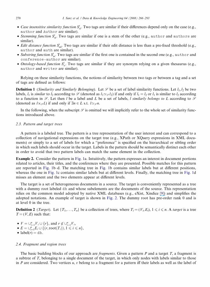
2.4. Fragment and region trees

The basic building blocks of our approach are fragments. Given a pattern P and a target T, a fragment isa subtree of T, belonging to a single document of the target, in which only nodes with labels similar to thosein P are considered. Two vertices u, v belong to a fragment for a pattern iff their labels as well as the label of

db[0,17,0,1]

article [1,16,1,1]

title[2,15,2,1]

authors[3,14,2,2]

editor[6,11,2,3]

name[5,12,3,2]

name[4,13,3,1]

name[8,9,2,1]

invited[9,8,2,2]

conference [7,10,1,2]

writer[13,4,1,3]

name[14,3,2,1]

article-title [15,2,2,2]

article-conference [16,1,2,3]

title[11,6,4,1]

author[12,5,4,2]

paper[10,7,3,1]

Fig. 2. A target.

I. Sanz et al. / Data & Knowledge Engineering 64 (2008) 266–293 271

their nearest common ancestor similarly belong to the labels in the pattern. Edges in the fragment either cor-respond to a direct edge in the target (father–children relationship) or to a path in the target (ancestor–descendant relationship). Several edges in the target, indeed, can be collapsed in a single edge in the fragmentby ‘‘skipping’’ nodes that are not included in the fragment since their labels do not similarly belong to thosein the pattern.

Definition 3 (Fragment). A fragment F of a target T = (VT,ET) for a pattern P is a subtree (VT,ET) of T forwhich the following properties hold:

• VF is the maximal subset of VT such that root(T) 62 VF and "u,v 2 VF, label(u), label(v), andlabelðncaðu; vÞÞ / labelðVðP ÞÞ;

• for each v 2 VF, nca(root(F),v) = root(F);• EF ¼ fðu; vÞju; v 2 V F ^ ðu; vÞ 2 E�T ^ ð 9=w 2 V F ;w 6¼ u; v s.t. ððu;wÞ 2 E�T ^ ðw; vÞ 2 E�T ÞÞg.

Example 3. Consider the pattern in Fig. 1a and the target in Fig. 2. By considering all the label similarityfunctions introduced in Section 2.2, the corresponding four fragments are shown in Fig. 3a. Labels in thefirst fragment are exactly the same appearing in the pattern. By contrast, in the others require to exploitthe substring and ontology-based functions. For instance, the second tree contains paper as label, andpaper ’St

oarticle. Similarly, the third and fourth trees contain node labels that are similar, exploiting

the substring function Stss to labels title and conference in the pattern, respectively. The second tree

provides an example of fragment in which a node of the original tree (i.e. node (9, 8,2,2) labeled byinvited) is not included.

Starting from fragments, regions are introduced as a combination of fragments rooted at the nearest com-mon ancestor in the target. Two fragments can be merged in a region only if they belong to the same docu-ment. In other words, the common root of the two fragments is not the db node of the target.

Example 4. Consider the tree T rooted at node n (13,4,1,3) in Fig. 2. It has two subtrees (the ones containingelements article-title and article-conference) that are fragments with respect to the pattern inFig. 1a. Though n is not (part of) a fragment, the subtree consisting of n and its fragment subtrees could have ahigher similarity with the pattern tree in Fig. 1a than its subtrees separately. Therefore, combining fragmentsinto regions may lead to subtrees with higher similarities.

article-conference [16,1,2,3]

article-title[15,2,2,2]

title[11,6,4,1]

paper[10,7,3,1]

conference [7,10,1,2]

article [1,16,1,1]

title[2,15,2,1]

article-title[15,2,2,2]

article-conference [16,1,2,3]

writer[13,4,1,3]

Fig. 3. (a) Fragments and (b) generated region.

272 I. Sanz et al. / Data & Knowledge Engineering 64 (2008) 266–293

A region can be a single fragment or it can be obtained by merging different fragments in a single subtreewhose root is the nearest common ancestor of the fragments. Thus, while all fragment labels similarly belongto those in the pattern, a region can contain labels not similarly belonging to pattern labels.

Definition 4 (Regions). Let FP(T) be the set of fragments identified between a pattern P and a target T. Thecorresponding set of regions RP(T) is inductively defined as follows:

• FP(T) � RP(T);• For each F = (VT,ET) 2 FP(T) and for each R = (VR,ER) 2 RP(T) s.t. label(nca(root(F),root(R))) 5 db,

S = (VS,ES) 2 RP(T); where:– root(S) = nca(root(F),root(R)),– VS = VF [ VR [ {root(S)},– ES = EF [ ER [ {(root(S),root(F)),(root(S),root(R))}.

Example 5. The fragments in Fig. 3a are also regions as well as the region reported in Fig. 3b obtained bymerging the third and fourth fragments in Fig. 3a. Note that the region root label (i.e. writer) does not sim-ilarly belong to any label in the pattern.

Relying on this definition, regions are all possible combinations of fragments in a document of the target.This number can be exponential in the number of fragments. In Section 4.3 the locality principle will be dis-cussed to reduce the number of regions to consider.

The notions of level of a node and distance between two nodes, when applied to regions, refer to thecorresponding notions in the original target tree. More specifically, they refer to the target subtree whoseroot is the region root and whose leaves are the region leaves. We will refer to this tree as the target subtreecovered by the region. This subtree, as already discussed, may contain additional internal nodes that arenot included in the region since their labels do not appear in the pattern. Specifically, internal nodes areincluded in the covered subtree if they are either in the path from the region root to some region node orif they are internal sibling of two nodes in the covered tree (i.e. right-sibling of one of them and left-siblingof the other).

Definition 5 (Covered Subtree). Let T be a target and R be a region on it. The subtree of T covered by R,denoted as C(R), is the subtree of T such as:

• VC(R) � VT is inductively defined as follows:– VR � VC(R);– "v 2 VT such that $u,w 2 VC(R) and (u,v), (v,w) 2 VT, v 2 VC(R);– "v 2 VT such that $u,w,f 2 VC(R) and (f,u),(f,v),(f,w) 2 VT, u is a left-sibling of v, and w is a right-sibling

of v, v 2 VC(R);• EC(R) = {(u,v)|(u,v) 2 ET s.t. u,v 2 VC(R)}.

I. Sanz et al. / Data & Knowledge Engineering 64 (2008) 266–293 273

Example 6. Consider region R2 of Fig. 5. The depth of the region level(R2) = 4 though the region includes only

three nodes. Similarly, the level of the paper labeled node is 3. The distance of the paper labeled node is 4,which is also the maximal distance in the region.

Fig. 4 presents different parts of a target where black nodes identify region nodes and gray nodes togetherwith black nodes form the covered subtree.

3. Similarity of a region w.r.t. a pattern

In this section we present the foundation of our two-phase approach to identify target regions similar to apattern. We first identify the possible matches between the vertices in the pattern and those in the region hav-ing similar labels, without exploiting the hierarchical structure of the tree. Then, the hierarchical structure istaken into account to select, among the possible matches, those that are structurally more similar. Specifically,after having introduced the definition of mapping, we propose three different similarity measures that combinestructure and tag matching.

3.1. Mapping between a pattern and a region

A mapping between a pattern and a region is a relationship among their elements that takes the tags used inthe documents into account. Our definition differs from the definition of mapping proposed by other authors[10,11]. Since our focus is on heterogeneous semi-structured data, we do not take the hierarchical organization

Fig. 4. Covered subtrees in a target.

article[1,16,1,1]

title[2,15,2,1]

article-title[15,2,2,2]

article-conference [16,1,2,3]

writer[13,4,1,3]

article

title conference

conference [7,10,1,2]

paper[10,7,3,1]

title[11,6,4,1]

R1

R2R3

Fig. 5. Mapping between the pattern and different regions.

274 I. Sanz et al. / Data & Knowledge Engineering 64 (2008) 266–293

of the pattern and the region into account in the definition of the mapping. We only require that the elementlabels are similar.

Definition 6 (Mapping M). Let P be a pattern and R be a region. A mapping M is a partial injective functionbetween the vertices of P and those of R such that 8xp 2VðP Þ;MðxpÞ 6¼?) labelðxpÞ ’ labelðMðxpÞÞ.

Example 7. Fig. 5 reports the pattern P of Fig. 2 in the center and three target regions, R1,R2, R3. Dashed linesrepresent a mapping among the vertices of the pattern and those of each region.

Several mappings can be established between a pattern and a region. The best one will be selected by meansof a similarity measure that evaluates the degree of similarity between the two structures relying on the degreeof similarity of their matching vertices.

Example 8. Fig. 6 reports how different mappings can be established between the region R in Fig. 3b and thepattern P in Fig. 1a.

Given a similarity measure, like the ones discussed in the next section, assessing the similarity between ver-tices, a mapping can be evaluated as follows.

Definition 7 (Evaluation of a Mapping M). Let M be a mapping between a pattern P and a region R, and letSim be a vertex similarity function. The evaluation of M is:

EvalðMÞ ¼P

xp2VðPÞs:t:MðxpÞ6¼?Simðxp;MðxpÞÞjVðP Þj

Similarity between a pattern and a region is then defined as the maximal evaluation among the mappingsthat can be determined between the pattern and the region.

Definition 8 (Similarity between a Pattern and a Region). Let M be the set of mappings between a pattern Pand a region R. The similarity between R and P is defined as:

SimðP ;RÞ ¼ maxM2M

EvalðMÞ

3.2. Similarity between matching vertices

We now present three approaches for computing the similarity between a pair of matching vertices. Thefirst one assesses similarity only on the bases of label matches, whereas the other two take the structure intoaccount.

article

title conferencearticle-title[15,2,2,2]

article-conference [16,1,2,3]

writer[13,4,1,3]

article-title[15,2,2,2]

article-conference [16,1,2,3]

writer[13,4,1,3]

article-title[15,2,2,2]

article-conference [16,1,2,3]

writer[13,4,1,3]

Fig. 6. Identification of different mappings from the same region and pattern.

I. Sanz et al. / Data & Knowledge Engineering 64 (2008) 266–293 275

3.2.1. Match-based similarity

In the first approach, similarity only depends on node labels. Similarity is 1 if labels are identical, whereas apre-fixed penalty d is applied if labels are similar. If they are not similar, similarity is 0.

Definition 9 (Match-based Similarity). Let P be a pattern, R be a region in a target T, xp a node of P, andxr = M(xp). Their similarity is computed as:

TableSimila

x1r

x2r

x3r

TableEvalua

M1

M2

Mb3

Ml3

Mr3

SimMðxp; xrÞ ¼1 if labelðxpÞ ¼ labelðxrÞ1� d if labelðxpÞ ’ labelðxrÞ0 otherwise

8><>:

Example 9. Let xp be the vertex tagged article in the pattern P in Fig. 5 and x1r ; x

2r ; x

3r the corresponding

vertices in the regions R1, R2, R3. Table 2a reports, in the first column, the match-based similarity betweenxp and the corresponding vertices in the three regions.Table 2b reports, in the first column, the match-basedevaluations of the mappings between P and each of the regions (see Fig. 5), computed according to Definition7. For regions R1 and R2, there is a single mapping (M1 and M2, respectively). For region R3, by contrast, thethree mappings Ml

3, Mr3, and Mb

3, appearing in the left, right, and bottom of Fig. 6, are evaluated. The tablealso highlights in bold the similarity of P with each of the regions, computed according to Definition 8. Theevaluation details are in Appendix A.

3.2.2. Level-based similarity

In the second approach, the match-based similarity is combined with the evaluation of the level at which xp

and M(xp) appear in the pattern and in the region. Whenever they appear in the same level, their similarity isequal to the similarity computed by the first approach. Otherwise, their similarity linearly decreases as thenumber of levels of difference increases. We recall that levels in the region refer to the levels in the target sub-tree covered by the region.

Definition 10 (Level-based similarity). Let P be a pattern, R be a region in a target T, xp a node of P, andxr = M(xp). Their similarity is computed as:

SimLðxp; xrÞ ¼ SimMðxp; xrÞ �jlevelP ðxpÞ � levelRðxrÞjmaxðlevelðP Þ; levelðRÞÞ

The similarity is 0 if the obtained value is below 0.

Example 10. The second columns of Tables 2a and 2b report the level-based similarities. The evaluationdetails are in Appendix A.

2arity of matching vertices

SimM SimL SimD

1 1 11 � d 1

2� d 12� d

1 � d 12� d 1

3� d

2btion of mappings and similarity of a pattern with regions

SimM SimL SimD

23

23

23

1� d3

712� d

312� d

323 � ð1� dÞ 1

2� 23 � d 1

2� 23 � d

23 � ð1� dÞ 1

2� 23 � d 5

9� 23 � d

23 � ð1� dÞ 2

3 � ð1� dÞ 23 � ð1� dÞ

Fig. 7. Distance of a vertex in a region R.

276 I. Sanz et al. / Data & Knowledge Engineering 64 (2008) 266–293

3.2.3. Distance-based similarity

Since two nodes can be in the same level, but not in the same position, a third approach is introduced. Thesimilarity is computed by taking the distance of nodes xp and M(xp) with respect to their roots into account.Thus, in this case, the similarity is the highest only when the two nodes are in the same position in the patternand in the region. We recall that distances in the region refer to the distances in the target subtree covered bythe region computed through the recursive function dR in Fig. 7. Given a region R, v1, . . . ,vn are the vertices ofR ordered according to their pre-order rank in the target T. In the figure we report the computation of thedistance for the root of R (v1) and for a generic vertex of R that is not the root. Note that, dmax

R ¼ dRðvnÞ. Giventwo adjacent vertices vi�1 and vi that are not siblings, avi�1 and avi denote their common sibling ancestors. Weremark that the last expression for computing the distance of a generic vi in R includes the two previous casesin the definition of dR. However, for the sake of clarity we have pointed out these two particular cases.

Definition 11 (Distance-based Similarity). Let P be a pattern, R be a region in a target T, xp a node of P, andxr = M(xp). The similarity is computed as:

SimDðxp; xrÞ ¼SimMðxp; xrÞ �jdP ðxpÞ � dRðxrÞjmaxðdmax

P ; dmaxR Þ

The similarity is 0 if the obtained value is below 0.

Example 11. The third columns of Tables 2a and 2b report the distance-based similarities. The evaluationdetails are in Appendix A.

4. Construction of fragments and regions

The focus of this section is on the data structures and algorithms for the efficient identification of fragmentsand regions in the target. As specified in Definition 3, each fragment is a set of nodes bound by the ancestor–descendant relationship in the target. A general purpose indexing structure along with an indexing structuredepending on the pattern P are employed for improving the performances of our approach. Fragments aremerged into regions, as specified in Definition 4, only when the similarity between P and the generated regionis greater than the similarity between P and each single fragment. Target subtrees covered by a region shouldbe evaluated only accessing nodes in the regions and information contained in the auxiliary indexingstructures.

In the remainder of the section, we first present the indexing structures. Then, we discuss the algorithms forthe construction of a list of fragments and for the creation of regions starting from such a list.

4.1. Similarity-based inverted index and pattern index

Directly evaluating the pattern on the target is inefficient and introduce scalability issues in the approach,due to the tag and structural heterogeneity of the collection. For these reasons, a similarity-based inverted

index (SII) is proposed. This index is independent from the retrieval pattern and is composed by a traditional

I. Sanz et al. / Data & Knowledge Engineering 64 (2008) 266–293 277

inverted index coupled with a table, name-similarity table, that specifies relationships among tags in the col-lection relying on the semantic functions discussed in Section 2.

This index allows us to easily identify in the collection nodes with similar tags according to different criteria.Since the number of labels that normally occur in a target is sensibly smaller than the number of elements, thesize of the name-similarity table is often contained and it can also fit in main memory.

The SII index is built as follows. Starting from the labels of a target T, a traditional inverted index is cre-ated, that is, each distinct label l occurring in the target is associated with the list of vertices labeled by l,ordered according to the pre-order rank. The 5-tuple ðpreðvÞ; postðvÞ; levelðvÞ; posðvÞ;PðvÞÞ is maintainedfor each vertex v 2VðT Þ. Then, tags in the collection are grouped according to each of the tag-based similar-ity functions presented in Section 2 and each group is progressively numbered. Each tag is finally associatedwith the list of the group identifiers it belongs to. Fig. 8b reports this association by means of a table. Forexample, author and authors belong to the same class according to function St

ed, whereas author,authors, and writer belong to the same class according to function St

o. In this way, when nodes taggedl should be retrieved in the target, the rows in the name-similarity table corresponding to l are extracted,and then, according to one or more similarity measures, all the similar tags are easily identified. In the casel does not belong to the name-similarity table, one of the tag-based similarity functions can be applied to iden-tify a similar tag in the table.

Given a pattern P, for every node v in P, all the occurrences of nodes u in the target tree such thatlabelðvÞ’SlabelðuÞ are retrieved from the SII index according to the functions in S, and organized level bylevel in a pattern index. The pattern index therefore depends on the pattern that should be evaluated onthe target. The number of levels in the index depends on the levels in T at which vertices occur with labelssimilar to those in the pattern. For each level, vertices are ordered according to the pre-order rank.

Depending on the label similarity functions in S, different pattern indexes can be generated. Fig. 9a showsthe pattern index obtained by identifying nodes identical to those of the pattern, Fig. 9b reports the patternindex obtained by applying the ontology-based function St

o, and, finally, Fig. 9c the pattern index in which allthe criteria have been exploited. All the pattern indexes are obtained starting from the pattern in Fig. 1a eval-uated on the SII index in Fig. 8 corresponding to the target in Fig. 2.

1,16,1,1

4,13,3,1

15,2,2,2

10,7,3,1

16,1,2,3

5,12,2,2

12,5,2,2

3,14,2,2

13,4,1,3

7,10,1,2

14,3,2,18,9,2,1

6,11,2,3

9,8,2,2

article

author

article-title

paper

name

conference

invited

editor

article-conference

authors

writer

title

Sedt

Ssst

Sott

Sci

1

2

1

2

2

1

1

1

2

2

3

3

1

1

11,6,4,12,15,2,1

articlearticle-title

tag

article-conference

article-title

author

papername

conference

invited

editor

authors

writertitle

article-conference

tSst

1

1

Fig. 8. SII index components: (a) inverted index and (b) name-similarity table.

1,16,1,1 7,10,1,2

2,15,2,1

1

2

3 11,6,4,1

1,16,1,1 7,10,1,2

10,7,3,1

11,6,4,1

1

2

3

4

2,15,2,1

1,16,1,1

15,2,2,2 16,1,2,3

7,10,1,2

10,7,3,1

11,6,4,1

1

2

3

4

2,15,2,1

Fig. 9. Pattern index (a) with label equality, (b) applying ontology-based function, and (c) applying all the criteria.

278 I. Sanz et al. / Data & Knowledge Engineering 64 (2008) 266–293

The construction of the pattern index requires to identify the entries in SII with similar tags to those of P.For each node of P, this operation requires (in the worst case) to check the distinct labels that tag each entry ofSII. Once the entries are identified, the corresponding nodes are inserted in the pattern index. Since the nodesin each entry are ordered according to the pre-order rank in the target, the construction of the pattern index isperformed in linear time. Therefore, the number of operations for each tag in P is in the order of OðK �MÞwhere K is the number of entries and M the maximal number of nodes in each entry. The number of opera-tions for the construction of the entire pattern index for a pattern P is thus OðjP j � K �MÞ. We remark that theuse of the name-similarity table does not affect the complexity of the approach in the worst case analysis butonly in the average case.

Algorithm 1: Create Fragments

Require: PI,F,v,l{PI: pattern indexF: current fragmentv: vertex in current fragmentl: a level in the pattern index}SF = ;if l 6 size(PI) ^ head(PI(l)) is not null then

while head(PI(l)) is not null and precedes root(F) do

Create a new fragment F 0 = (V0F ,;) such that V0F = {head(PI(l))}SF = SF [ {F 0} [ createFragments(PI,F 0,head(PI(l)),l + 1)remove head(PI(l))

end while

while head(PI(l)) is not null and is a descendant of (root(F)) do

Insert head(PI(l)) in the vertex of F

if head(PI(l)) precedes v then

Insert (root(F), head(PI(l))) in the edges of F

else

Insert (v, head(PI(l))) in the edges of F

end if

SF = SF [ createFragments(PI, F, head(PI(l)), l + 1)remove head(PI(l))

end while

SF = SF[ createFragments(PI, F, v, l + 1)end if

Ensure: return SF

4.2. Algorithms for the construction of fragments

Once the pattern index is generated, the fragments are generated through the recursive Algorithm 1: Cre-

ateFragments and Algorithm 2: CreateListOfFragments. The main advantage of these algorithms is the iden-

I. Sanz et al. / Data & Knowledge Engineering 64 (2008) 266–293 279

tification of the fragments through a single visit of the pattern index so that the complexity of fragments con-struction is kept linear.

To simplify the presentation of the algorithm we assume that, once a node in the pattern index is visited andinserted in a fragment, it is removed from the pattern index. In the algorithms, given a pattern index PI,size(PI) denotes the number of levels, PI(l) denotes the list of nodes at level l (1 6 l 6 size(PI)), and head(PI(l))denotes the first node in the list PI(l).

Algorithm CreateFragments is invoked relying on the level and the pre-order rank of the roots of the frag-ments to be generated. Given a fragment F, CreateFragments identifies all the nodes of F appearing in the pat-tern index and generates a tree on such nodes according to Definition 3. Moreover, the recursive calls of thisfunction also return the fragments whose roots appear in a lower level and precede the root of F.

Relying on the assumption that, when a fragment is generated it is removed from PI, the PI on which Cre-

ateFragments is invoked for a fragment F does not contain all the nodes belonging to fragments whose rootsare at a level k such that k < level(root(F)). After the invocation of CreateFragments on F, PI will not containall the nodes of F along with the nodes of the fragments whose roots precede root(F) at a level h such that(h > l).

Algorithm CreateFragments takes as input the pattern index PI, the current fragment F, a node v in F (ini-tially the root of F, then an internal node for which we are looking for direct descendants), and the level l in PI

where we are looking for descendants of F. Its behavior relies on the following proposition.

Proposition 1. Let CreateFragments be invoked for a fragment F on a level l of a pattern index PI and a leaf node

v of F located at a level m in PI(m < l). The following properties hold:

(1) If head(PI(l)) is a left relative of root(F), head(PI(l)) is the root of a new fragment.(2) If head(PI(l)) is a descendant of root(F), but not of v, head(PI(l)) belongs to F and is a descendant of

root(F).(3) If head(PI(l)) is a descendant of v in F, head(PI(l)) belongs to F and is a descendant of v.(4) If head(PI(l)) is a right relative of root(F), no elements of F can be identified at this level.

The cases described by Proposition 1 can occur in each invocation of Algorithm CreateFragments and han-dled as follows. We refer to Fig. 10 for a better understanding of the behavior of the algorithm. If head(-PI(l)) = t is left relative of root(F) (case (1) of Proposition 1), t is the root of another fragment. Indeed, allthe fragments Fo such that root(Fo) precedes root(F) at a level k (k < l) could contain t have been removedfrom PI. Therefore, a new fragment F 0 is created and Algorithm CreateFragments is invoked for this fragmentand its root at level l + 1. If head(PI(l)) = u belongs to the descendants of root(F), but it is not a descendant ofv (case (2) of Proposition 1), u is left relative of all internal nodes of F. Therefore, u is inserted as child ofroot(F) and Algorithm CreateFragments is invoked on F and u to identify possible descendants of u in F at

F

v

level lt u w x

sz

y

F’n

Fig. 10. Situations that can arise in the creation of a fragment.

280 I. Sanz et al. / Data & Knowledge Engineering 64 (2008) 266–293

level l + 1. If head(PI(l)) = w (the behavior is the same for node x) belongs to the descendants of v (case (3) ofProposition 1), w is associated as a child of v and Algorithm CreateFragments is invoked on F andw to identify possible descendants of w in F at level l+1 (as shown in Fig. 10 node z will be identified). Ifhead(PI(l)) = n is right relative of F (case (4) of Proposition 1), nor n nor the nodes that could follow n at levell can belong to F. Algorithm CreateFragments is thus invoked recursively on F, the same v and level l + 1 inorder to identify further descendants of v that do not stay at level l. Through this call, nodes y and s will beidentified if v is their immediate ancestor in F.

Starting from the root of a fragment F, Algorithm CreateFragments is recursively invoked on the levels ofthe pattern index between the level of root(F) and size(PI). Therefore, we are guaranteed that if a level con-tains a node of F, it is detected and inserted in the correct position in the hierarchical structure of F.

Algorithm CreateListOfFragments generates fragments starting from the first level of PI and moving down-wards to its last level. In the first level, all the nodes are roots of fragments. Therefore, Algorithm CreateFrag-ments is invoked on each of the fragments of the first level. Once all the fragments of the first level have beenidentified, the algorithm proceeds with the nodes of PI still belonging to the remaining levels (if they are notempty). Algorithm CreateListOfFragments ends when it reaches the last level of PI and all the nodes have beenremoved from PI.

Algorithm 2: Create List Of Fragments

Require:PI{PI = pattern index}SF = ;for l = 1 to size(PI)

while head(PI(l)) is not nullCreate a new fragment F = (VF,;) such that VF = {head(PI(l))}SF = SF [ {F}[ createFragments(PI,F,head(PI(l)),l + 1)remove head(PI(l))

end while

end for

Ensure return SF

Proposition 2. Let PI be the pattern index for a pattern P. Algorithm 2: CreateListOfFragments correctly

identifies all fragments in PI.

All the atomic operations in the algorithm (checking whether a node precedes another one, adding a nodeto a fragment, removing a node from PI) require a constant number of operations. The algorithm visits eachvertex in the pattern index only once by removing in each level the vertices already included in a fragment.Therefore, its complexity is in OðNÞ, where N is the number of nodes in PI.

Fig. 11 contains fragments F1, . . . ,F4 obtained from the PI of Fig. 9c.

15,2,2,2 16,1,2,31,16,1,1

2,15,2,1

7,10,1,2

10,7,3,1

11,6,4,1

(F1)

13,4,1,3

15,2,2,2 16,1,2,3

(F2) (F3) (F4) (R)

Fig. 11. Construction of fragments and regions.

I. Sanz et al. / Data & Knowledge Engineering 64 (2008) 266–293 281

4.3. Algorithm for the construction of regions

Two fragments should be merged in a single region when, relying on the adopted similarity function, thesimilarity of the pattern with the region is higher than the similarity with the individual fragments.

Whenever a document in the target is quite big and the number of fragments is high, the regions thatshould be checked can grow exponentially. To avoid such a situation we exploit the following locality prin-

ciple: merging fragments together or merging fragments to regions makes sense only when the fragments/regions are close. Indeed, as the size of a region tends to be equal to the size of the document, the similaritydecreases.

In order to meet such locality principle regions are obtained by merging adjacent fragments. Operatively,two adjacent fragments can be merged when their common ancestor v is not the root of the target. If it is notthe root of the target, their common ancestor v becomes the root of the region and the roots of the fragmentsbecome the direct children of v. We remark that the common ancestor of two fragments can be easily obtainedby traversing the P-arent link included in the nodes of the pattern index.

Combining the locality principle and the approach for merging together two adjacent fragments, Algorithm3: CreateListOfRegions is obtained. The algorithm works on the list of fragments SF obtained from AlgorithmCreateListOfFragments that is ordered according to the pre-order rank of the roots of the fragments it con-tains. Once a possible region Ri is obtained, by merging two adjacent fragments SF(i � 1) and SF(i), the sim-ilarity SimðP ;RiÞ is compared with the maximal value between SimðP ; SF ði� 1ÞÞ and SimðP ; SF ðiÞÞ. IfSimðP ;RiÞ is the highest, SF(i � 1) is removed from the list and SF(i) substituted with Ri. Otherwise, SF(i � 1)is kept alone and we try to merge SF(i) with its right adjacent fragment. The process ends when all the frag-ments in the list have been checked.

Algorithm 3: Create List Of Regions

Require SF, P{SF: list of fragmentsP: Pattern}for i = 2 to size(SF) do

Try to generate region Ri by merging SF(i � 1) and SF(i)if Ri has been generated then

if SimðP ;RiÞP maxfSimðP ; SF ði� 1ÞÞ;SimðP ; SF ðiÞÞg then

Remove SF(i � 1)Substitute SF(i) with Ri

end if

end if

end for

Ensure return SF

Example 12. Considering the running example we try to generate regions starting from the fragments inFig. 11. Since the common ancestor between F1 and F2 is the root of the target, the two fragments cannot bemerged. Same behavior for fragments F2 and F3. Since the common ancestor between F3 and F4 is a node inthe same document, region R in Fig. 11 is generated. Since the similarity of P with R is higher than itssimilarity with F3 and F4, R is kept and F3,F4 removed. At the end of the process we have regions {F1,F2,R}.

A key point of our approach is the efficient computation of the similarity between a pattern P and a frag-ment F or a region R. An array indexed on the labels of P is employed to keep the highest evaluation of sim-ilarity between a node in P and all the nodes in F/R with a similar label. The evaluation in the array are finallyadded to obtain the similarity between P and F/R. The number of operations is OðjP jÞ. Since the similaritybetween P and F can be computed during the construction of a fragment, the complexity for evaluatingthe similarity between P and F in this phase is constant. Things are different for the similarity between P

and R, where R is the combination of two fragments. In this case, the evaluations of two arrays should becompared and thus the number of operations is OðjP jÞ.

282 I. Sanz et al. / Data & Knowledge Engineering 64 (2008) 266–293

For the construction of a region a pair of fragments F1 and F2 must be considered. The arrays, associatedwith F1 and F2 containing the highest similarity between P and them, must be visited for obtaining the eval-uation of a region. Since the arrays have |P| entries and each fragment is considered only once, the number ofcomparisons is proportional to the size of the list of fragments. The number of operation is OðjP j � sizeðSF ÞÞ.Since in the worst case, each fragment contains a single node of the pattern index PI, size(SF) = size(PI).Therefore, the creation of regions from SF requires OðN � jP jÞ operations, where N is the number of nodesin PI.

We wish to remark that the construction of regions is quite fast because the target should not be explicitlyaccessed. All the required information are contained in the inverted indexes. Moreover, thanks to our locality

principle the number of regions to check is proportional to the number of fragments. Finally, the regionsobtained through our process do not present all the vertices occurring in the target but only those necessaryfor the computation of similarity. Vertices appearing in the region but not in the pattern are evaluated throughthe pre/post-order rank of each node.

Example 13. Consider the region R2 in Fig. 5 and the corresponding representation F2 in Fig. 11. Vertexinvited is not explicitly present in R. However, its lack can be taken into account by considering the levelsof vertex conference and vertex paper.

The following proposition summarizes the complexity of the algorithm for the creations of regions startingfrom a pattern.

Proposition 3. Let P be a pattern, K the number of distinct label in the SII index, and M the maximal size of an

entry in SII. Moreover, let N be the number of nodes in the pattern index PI. The number of operations for the

creation of regions starting from a pattern is OðmaxfðjP j � K �MÞ; ðN � jP jÞgÞ.

5. Prototype and experimental results

We have implemented a prototype using a Oracle Berkeley DB in the back-end, which is being used for theexploration of heterogenous sources in biomedical information integration projects. An example of this func-tionality is shown in two screenshots: Fig. 12 shows the combined results for a query and Fig. 13 shows the topresults found in different collections. The figure highlights the richness and heterogeneity of the retrieved struc-tures. This allows the data engineer to study the available collections as a whole, progressively refining thetargets and the measures. Note that the system allows tailoring the similarity measure on-the-fly; this case usesa domain-specific label-matching function (see Section 2.2).

We have used this system to experimentally evaluate, both on real and synthetic data, the following aspectsof our approach:

(1) Reasonable performance with large collections.(2) Handling of severe structural distortions.(3) Retrieval effectiveness in highly heterogeneous collections.

In the remainder of the section we report our results along these aspects.

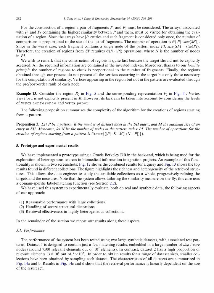
5.1. Performance

The performance of the system has been tested using two large synthetic datasets, with associated test pat-terns. Dataset 1 is designed to contain just a few matching results, embedded in a large number of don’t-care

nodes (around 7500 relevant elements out of 107 elements). In contrast, dataset 2 has a high proportion ofrelevant elements (3 · 105 out of 5 · 105). In order to obtain results for a range of dataset sizes, smaller col-lections have been obtained by sampling each dataset. The characteristics of all datasets are summarized inFig. 14a and b. Results in Fig. 14c and d show that the retrieval performance is linearly dependent on the sizeof the result set.

Fig. 12. Screenshot of the GUI prototype showing the top results in some collections, using a variation of the match-based similarity and aflexible label-matching function.

Fig. 13. Screenshot of the GUI prototype showing some results of a query over a set of heterogenous biomedical-related collections, usinglevel-based similarity and a flexible label-matching function.

I. Sanz et al. / Data & Knowledge Engineering 64 (2008) 266–293 283

1 2 3 4 5 6 7 8 9 10

Subcollection

Ele

men

ts

0e+

004e

+06

8e+

06

1 2 3 4 5

Subcollection

Ele

men

ts

0e+

002e

+05

4e+

050 2000 4000 6000

0.2

0.4

0.6

0.8

1.0

Nodes in result set

Que

ry ti

me

(s)

0 50000 150000 2500000

1020

3040

5060

Nodes in result set

Que

ry ti

me

(s)

Fig. 14. (a) Total number of elements in each subcollection extracted from dataset 1. (b) Total number of elements (n) and number ofrelevant elements ( ) in each subcollection extracted from synthetic dataset 2. (c) Execution time in dataset 1. (d) Execution time indataset 2.

284 I. Sanz et al. / Data & Knowledge Engineering 64 (2008) 266–293

5.2. Effect of structural distortions

The second aspect we have evaluated is the effect of structural variations in fragments. In order to test this,we have generated another synthetic dataset, in which we have embedded potential matches of a test patterncontaining 15 elements with the following kinds of controlled distortions: (1) addition of n random nodes; (2)deletion of n random nodes; (3) switching the order of nodes in the same level, with a given probability; (4)switching parent and child nodes, with a given probability.

Results in Fig. 15 show that the system is able to find all relevant fragments despite the introduced distor-tions. Predictably, only the removal of relevant nodes in the target has an effect in the average relevance ofresults. Adding nodes, switching nodes in the same level, and interchanging parent and child nodes haveno effects on the retrieval rate.

5.3. Retrieval in highly heterogeneous collections

In our third set of experiments we analyze the retrieval effectiveness in the context of highly heterogeneouscollections. Our goal is to evaluate the effectiveness of our approach according to different parameters, such asthe size of the data collection, its degree of vocabulary and structural heterogeneity, and its degree of confor-mance to the query.

We experimented on a set of document collections patterned after the highly heterogeneous ASSAM4 data-set. While the information content of the generated collections is the same of that of the real ASSAM, the newcollections are bigger and present different levels of heterogeneity and conformance to the queries. The gen-eration is based on empirical estimations of the relative probabilities of ASSAM’s main topics and entities.Since the queries present a tree structure as well, pattern generators have been employed for the automatic

4 http://moguntia.ucd.ie/repository/datasets/.

2 4 6 8 10

0.6

0.8

1.0

1.2

1.4

Nodes added

Ave

rage

sim

ilarit

y

2 4 6 8 10

0.5

0.6

0.7

0.8

0.9

Nodes removed

Ave

rage

sim

ilarit

y20 40 60 80 100

0.6

0.8

1.0

1.2

1.4

Odds of a change in parent/child node ordering

Ave

rage

sim

ilarit

y

20 40 60 80 100

0.6

0.8

1.0

1.2

1.4

Odds of a change in sibling node orderingA

vera

ge s

imila

rity

Fig. 15. Change in similarity with the addition and removal of nodes in regions.

I. Sanz et al. / Data & Knowledge Engineering 64 (2008) 266–293 285

construction of synthetic queries. The use of a probabilistic approach for the generation of queries simulatesthe users’ uncertainty about the structure of the target collection in query formulation.

To obtain quality measures such as precision and recall we need relevance assessments. These are manuallyevaluated on the original ASSAM collection. In the generated collections, query identifiers are linked to thepattern used for the generation of the collection, thus specifying which generated subtrees constitute a correctanswer for the query. This allows us to build collections of arbitrary size while being able to assess the rele-vance of each query answer.

In what follows, we first describe the generation of documents and queries and then present the experimen-tal results on the original collection and on the generated ones.

Generation of documents and queries. To generate suitable test collections and queries we have built a newsystem whose generation model significantly expands ToXgene [12] facilities, that only provides limited sup-port for ‘‘random structures’’, for the specification of heterogeneous contents.

Our collection generator provides a set of XML pattern constructors, which encapsulate different templatesfor generating XML structures. A generator pattern is itself an XML document, whose nodes represent bothpattern constructors and the tags to be generated. In general, the ancestor/descendant relationships betweenthese tags will be preserved in the generated documents. Each node in a generator pattern may have associateda probability indicating the likelihood of finding the subtree it represents in the generated documents (if omit-ted, the probability is taken to be 1.0). Thus, if node u is a child of node v, then P(u|v) = P(u) Æ P(v|v 0), where v 0

is the parent of v. If u is the pattern root node, then P(u) is the probability of the whole pattern. This simplemodel supports a wide variety of possible heterogeneous structures; Table 3 shows the main pattern construc-tors available.

Table 4 shows the summary of the generation patterns used in our experiments. They mainly reflect thefeatures of the ASSAM dataset. As this dataset is mainly a semi-structured representation of a set of web ser-vices, their structures are quite heterogeneous and tag names also present many variations. In this collection,tag names are usually phrases that combine in some way the key concepts of the web service. This feature hasbeen simulated using the a:combi pattern constructor, estimating n-gram probabilities from ASSAM data.This has been simulated by introducing subpatterns with the constructor a:subPattern. In Table 4 the lastcolumn indicates the used subpatterns in each generator pattern. Two sample generators models are shown inFig. 16.

Table 3Constructors for pattern generators

Constructor Pattern examples Generated XML

a:genPattern ha:genPattern a:id=’1’ihaddress/ih/a:genPatterni

haddress/i

sequence ht1iha:sequenceiha/ihb/ih/a:sequenceih/t1i

ht1iha/ihb/ih/t1i

xor ht1 a:xor=’yes’iha/ihb/ih/t1i

(a) ht1iha/ih/t1i(b) ht1ihb/ih/t1i

combi ha:combiiha/ihb/ih/a:combii

a) ha_b/ib) ha/ic) hb/i

if-ancestor ha:if-ancestor a:name=’t1’ihtag2/ih/a:if-ancestori

ht1i. . .htag2/i. . .h/t1i

types hperson a:types=’user,client’/i a) huserib) hpersonic) hclienti

dmin, dmax a) ht1iht2 a:dmin=’0’ a:dmax=’0’/ih/t1ib) ht1iht2 a:dmin=’2’ a:dmax=’2’/ih/t1i

a) ht1_t2ib) ht1_t2iht1ihkjkkijiht2/ih/kjkkijih/t1ih/t1_t2i

a:subPattern ht1iha:subPattern a:id=’1’/ih/t1i ht1ihaddress/ih/t1i

Table 4Database and query patterns used in experiments

Pattern ID Tags Depth Uses

Database patterns

Weather info BD-1 31 4 AddressPostal address BD-2 14 4 –Stock quotes BD-3 16 4 –Bank info BD-4 9 8 Address, StockCredit card BD-5 8 3 Bank InfoPersonal data BD-6 19 8 Address, Bank Info

Query patterns

Weather Q-1 12 3 –ZIP codes Q-2 3 1 –PostBox Q-3 3 1 –Quotes Q-4 5 2 –Bank code Q-5 3 1 –ATM location Q-6 3 2 AddressContact person Q-7 5 2 –Employee salary Q-8 3 2 –Credit card Q-9 3 2 –User account Q-10 4 2 –

286 I. Sanz et al. / Data & Knowledge Engineering 64 (2008) 266–293

a.genPatternid=3

name=stock

Stocka:query=4

Quotesa:query=4a:dmax=0

0.7

Name

0.6

Number

0.2

Quotea:query=4xor=yes

0.8

Market_Capitalization

0.2

Amount_Stocks

0.2

Change

0.6

a.combi

Weeklya:query=4

0.3

Daya:query=4a:dmax=0

0.4

Currenta:query=4

0.3

Range

0.7

Lowa:dmin=0

Higha:dmin=0

Lowa:dmin=0

Higha:dmin=0

Open Close

Percentagedmax=0

0.9

Tickera:query=4

0.7

Symbola:query=4

0.8

a.genPatternid=3

name=QueryStock

a.queryid=4

Stock

Ticker_Symbol Quote

a.xor

Weekly

0.2

Day

0.3

Current

0.5

Fig. 16. (a) Generator for database pattern 3. (b) Generator for query 4, associated with pattern 3.

1 2 3 4 5 6 7 8 9 10

Precision (distance–strict)

0.0

0.2

0.4

0.6

0.8

1.0

1 2 3 4 5 6 7 8 9 10

Precision (distance–partial)

0.0

0.2

0.4

0.6

0.8

1.0

1 2 3 4 5 6 7 8 9 10

Recall (distance–strict)

0.0

0.2

0.4

0.6

0.8

1.0

1 2 3 4 5 6 7 8 9 10

Recall (distance–partial)

0.0

0.2

0.4

0.6

0.8

1.0

1 2 3 4 5 6 7 8 9 10

F1measure (distancestrict)

0.0

0.2

0.4

0.6

0.8

1.0

1 2 3 4 5 6 7 8 9 10

F1measure (distancepartial)

0.0

0.2

0.4

0.6

0.8

1.0

Fig. 17. Precision, recall and F1 for measure distance, using strict and partial label matching. For each of the 10 queries, the darker bars(n) are computed using only the highest-ranked 10 results, the lighter bars ( ) consider all the returned matches.

I. Sanz et al. / Data & Knowledge Engineering 64 (2008) 266–293 287

288 I. Sanz et al. / Data & Knowledge Engineering 64 (2008) 266–293

Results on the generated documents and queries. The generated queries were evaluated against a generatedcollection of 50000 documents, with a total of one million nodes and around five thousand unique labels(around 500 times larger than the original ASSAM). Given the characteristics of the collection, we selectedthe following parameters for the experiments:

• We compared the performance of strict label matching with a partial matching function adapted to thecharacteristics of the collection as described above. The resulting partial matching function combines mostof the similarity functions described in Section 2.2.

• We used the structural distance similarity measure described in Section 3.2, with d = 0.1; the resultsobtained with the level measure were similar for this particular collection.

Fig. 17 shows the precision, recall and F1-measure, as well as the precision@10, recall@10 and F1@10 (i.e.the values express the 10 highest-ranked results).

The results under these experimental conditions can be summarized as follows:

• Setting the cutoff at 10 produces much better results than considering all the results. There is an exceptionfor query 3; a closer analysis of this particular case shows that query 3 contains very ambiguous tags, pro-ducing a large set of irrelevant results despite the use of tag similarity functions.

• As expected, the results obtained using strict label matching produce a better precision than those obtainedusing partial label matching, while partial matching produces better recall. Overall, the F1 measure is gen-erally better for strict matching on all the results, but the combination of 10-highest ranked and partialmatching is the best combination.

Results on the original ASSAM collection. Analogous queries were evaluated against the original ASSAMcollection, and the relevance of the results checked by hand. A summary of the results is shown in Fig. 18. Thefirst column indicates the query number, and the second column indicates the similarity threshold used for theanswer set (we used an explicit cutoff percentage MinSim instead of selecting the k highest results due to therelatively small size of the collection). The results are closely related to those obtained in our more generalexperimental setting, including the low F1 for query Q3.

6. Related work

The need of shifting from exact queries with boolean answers to proximity queries with ranked approxi-mate results is a relevant requirement of XML query languages for searching the Web and several approachesin this direction have been developed. These approaches share the goal of integrating structural conditionstypical of database queries with weighted and ranked approximate answers typical of Information Retrieval(IR). Work from the IR area [13] is mainly concerned with the retrieval of XML documents, by representingthem with known IR models. These approaches mainly focus on the textual part of XML documents andstructure is only used to guide user queries.

A crucial issue in ranked approximate querying is how to score results. A great variation of XML similaritymeasures have been proposed for different applications (see [14,15] for a survey). In this section, we will brieflydiscuss the similarity measures the most meaningful approaches to XML approximate querying rely on torank results. Further specific structural similarity measures have been proposed in the areas of Schema Match-

Fig. 18. Results for the ASSAM datasets.

I. Sanz et al. / Data & Knowledge Engineering 64 (2008) 266–293 289

ing [16] and more recently Ontology Alignment [17]. In the former, tree/graph-matching techniques allowdetermining which schema portions from the target schema can be mapped to the source ones. In this context,data types and domain constraints are used to decide if two nodes match. However, schemas usually exhibitsimple structures that seldom exceed three depth levels (relation-attribute-type). In the latter, the problem con-sists in finding out which concepts of a target ontology can be associated to concepts of the source ontology.

In this section, we focus on approximate query answering for XML documents taking both vocabulary andstructural heterogeneity into account. First, we discuss the kind of heterogeneity taken into account and thesimilarity measures employed to score results. Then, algorithmic approaches to query relaxation and to com-pute the top-k results are reviewed.

Heterogeneity degree and similarity evaluation. An early approach for XML approximate retrieval isELIXIR [18] that allows approximate matching in data content (tree leaves), and ranks the results accordingto the matching degree, disregarding structure in the evaluation. No structural heterogeneity is considered,and vocabulary heterogeneity is allowed only for data content elements, not for tags.

More sophisticated approaches, like XIRQL [19] and XXL[20], accept approximate matching at nodes andthen discuss how to combine weights depending on the structure. Vocabulary heterogeneity is supported forcontent and element tags, but no structural heterogeneity is allowed: conditions on document structure areinterpreted as filters, thus they need to be exactly satisfied. XXL supports a similarity operator and, to usethis operator, the user should be aware of the occurrence of similar keywords or element tags.

In the approach proposed by Damiani and Tanca [21] both XML documents and queries are modeled asgraphs labeled with fuzzy weights capturing the information relative relevance. They propose to employ bothstructure related weighting (weight on an edge) and tag related weighting (weight on a node). Some criteria forweighting are proposed such as the weight decreases as moving far away from the root, the weight depends onthe dimension of the subtree. Shortcut edges are considered, thus allowing the insertion of nodes, which weightis function of weights of edges. The match score is a normalized sum of weight of edges.

In the tree relaxation approach [2] exact and relaxed weights are associated with query nodes and edges.The score of a match is computed as the sum of the corresponding weights, and the relaxed weight is functionof the transformations applied to the tree. The considered transformations are: relax node, replacing the nodecontent with a more general concept; delete node, making a leaf node optional by removing the node and theedge linking it to its parent; relax edge, transforming a parent/child relationship to an ancestor/descendantrelationship; promote node, moving up in the tree structure a node (and the corresponding subtree).

The approXQL [5] approach can also handle partial structural matchings. All the paths in the query arehowever required to occur in the document. The allowed edit operations on the document tree are delete node,insert intermediate node, relabel node. The score of match is function of the number of transformations, eachone of which is assigned with a user-specified cost.

Amer-Yahia et al. in [3] account for both vocabulary and structural heterogeneity and propose scoringmethods that are inspired by tf*idf and rank query answers on both structure and content. Specifically, twigscoring accounts for all structural and content conditions in the query. Path scoring, by contrast, is an approx-imation of twig scoring that loosens the correlations between query nodes when computing scores. The keyidea in path scoring is to decompose the twig query into paths, independently compute the score of each path,and then combine these scores.

Table 5Heterogeneity degree in XML approximate querying

Vocabulary heterogeneity Structural heterogeneity Ranking

ELIXIR On content – Structure independentXIRQL On content – Structure dependentXXL On content and tag – Structure dependent[21] On content and tag Node insertion Structure dependent[2] On content and tag Delete node, relax edge, promote node Structure dependentapproXQL On content and tag Node insertion, node deletion Structure dependent[3] On content and tag Edge generalization, leaf deletion, subtree promotion Structure dependent

290 I. Sanz et al. / Data & Knowledge Engineering 64 (2008) 266–293

The main differences among the considered approaches are summarized in Table 5. Note how approachesto XML approximate queries have progressively shifted to higher degrees of heterogeneity, and to cope alsowith structural heterogeneity. Our approach allows for more significant structural variations and can be con-sidered as a step forward in the treatment of structural heterogeneity in the context of XML. All the consid-ered approaches, indeed, enforce at least the ancestor–descendant relationship in pattern retrieval, whereasour approach also allows to invert and relax this relationship. Our approach, moreover, is highly flexiblebecause it allows choosing the most appropriate structural similarity measures according to the applicationsemantics.

Tree embedding and top-k processing. A different perspective from which approaches to XML approximatequerying started, is that of looking for approximate structural matches, allowing the structure of the docu-ment and query trees to partially match. Kilpelainen [1] discusses ten different variations of the tree inclusionproblem, that is, the problem of locating instances of a query tree Q in a target tree T. He orders these differentproblems, ranging from unordered tree inclusion to ordered subtrees, highlighting the inclusion relationshipsamong them. Moreover, he gives a general schema of solution, and instantiates it for each problem, discussingthe resulting complexities. His goal, however, is not to measure the distance, nor to rank results. All theinstances of the pattern in the data tree are returned.

Another approach aimed at identifying the matches but that does not rank them, is by Kanza and Sagiv[22]. They advocate the need of more flexible query evaluation mechanisms in the context of semi-structureddata, where both queries and data are modeled as graphs. They propose mapping query paths to data paths,so long as the data path includes all the labels of the query path; the inclusion needs not to be contiguous or inthe same order.

Sub-optimal approaches for ranked tree-matching have been proposed for dealing with the NP complexityof the tree inclusion problems widely discussed and analyzed in [1]. In these approaches, instead of generatingall (exponentially many) candidate subtrees, the algorithms return a ranked list of ‘‘good enough’’ matches.For example, in [23] a dynamic programming algorithm for ranking query results according to a cost functionis proposed. In [2] a data pruning algorithm is presented where intermediate query results are filtered dynam-ically during evaluation process. ATreeGrep [24], instead, uses as basis an exact matching algorithm, butallowing a fixed number of ‘‘differences’’ in the result. [4] proposes an adaptive query processing algorithmto evaluate approximate matches where approximation is defined by relaxing XPath axes. In adaptive queryprocessing, different plans are permitted for different partial matches, taking the top-k nature of the probleminto account.

Starting from the user query, the approaches [2–5], for structural and content scoring of XML documents,generates relaxations of the query structure that preserve the ancestor–descendant relationships existingamong nodes in the query. These relaxations do not consider the effective presence of such a structure inthe collection of documents. The number can also be really high when the number of nodes in the query ishigh. The novelty of our approach relies on the employment of ad-hoc indexing structures. By exploiting suchauxiliary information, only the variations on the pattern that occur in the target are considered. The numberof variations to be evaluated is thus considerably reduced, still allowing for greater structural heterogeneity, asdiscussed in the previous section. Finally, in [2–5] constraints in the user queries are relaxed to augment theobtained results, whereas in our approach, we start from a completely relaxed query. We follow this approachbecause of the high degree of heterogeneity of the collection of documents we work on and we apply indexingstructures for improving the performance.

7. Conclusions and future work

In this paper we have developed an approach for the identification of subtrees similar to a given pattern in acollection of highly heterogeneous semi-structured documents. In this context, the hierarchical structure of thepattern cannot be employed for the identification of the target subtrees but only for their ranking. Peculiaritiesof our approach are the support for tag similarity relying on a thesaurus, the use of indexing structures toimprove the performance of the retrieval, and a prototype of the system.

As future work we plan to compare different similarity measures in order to identify those more adequatedepending on the application context and the heterogeneity of the considered data. Such measures can be col-

I. Sanz et al. / Data & Knowledge Engineering 64 (2008) 266–293 291

lected in a framework of functions that a user can select, compose, and apply depending on her needs. More-over we plan to consider more sophisticated patterns in which further constraints on vertices and edges can bestated. For instance, an element or a portion of the pattern could be requested to mandatorily appear in thetarget regions, or the difference between the levels in which two elements appear could be constrained by fixinga threshold. The constraints should then be considered in the similarity evaluation. Finally, we wish to con-sider subtree identification in a collection of heterogeneous XML Schemas. In this context, the proposedapproach should be tailored to the typical schema constraints (e.g., optionality and repeatability of elements,groups, types).

Appendix A. Details of similarity evaluation

Detailed match-based similarity (see Example 9). Let xp be the vertex tagged article in the pattern P inFig. 5 and x1

r ; x2r ; x

3r the corresponding vertices in the regions R1, R2, R3. In R1, article appears with the

same label then the match-based similarity is 1, whereas in the other two regions a similar tag appears, thenthe match-based similarity is 1 � d.

Consider now Table 2b. Since R1 has two perfect node matches over three nodes in the pattern, theresulting similarity is 2

3. Region R2 has two perfect matches and a similarity match, over three nodes in

the pattern, thus the resulting similarity is 3�d3

. All the three mappings with region R3 have two similaritymatches and no exact matches over three nodes in the pattern, thus the resulting similarity is 2

3� ð1� dÞ

in all cases.Detailed level-based similarity (see Example 10). In Table 2a, the level-based similarity is 1 for region R1

because the vertex tagged article in that region appears at the same level it appears in the pattern. Bycontrast, the level-based similarity between xp and x2

r is 12� d because their labels are similar there are two

levels of difference (the level of x2r is 3 and the level of xp is 1) and the maximal number of levels in P and

R2 is 4. The level-based similarity between xp and x3r is 1

2� d because their labels are similar there is one

level of difference (the level of x3r is 2 and the level of xp is 1) and the maximal number of levels in P and

R3 is 2.Consider now Table 2b. Since R1 has two perfect (both tags and levels coincide) node matches over three

nodes in the pattern, the resulting similarity is 23. Consider now region R2. The similarities are: 1

2� d for node

labeled article, 12

for node labeled title, and 34

for node labeled conference, thus resulting in 712� d

3. For

region R3, the bottom mapping in Fig. 6 results in 12� d for node labeled article and 1 � d for node labeled

title, thus in 12� 2

3� d overall similarity. The left mapping in Fig. 6 yields to the same similarity. By contrast,

the right mapping in Fig. 6 yields to 1 � d both for node labeled article for node labeled title, thus in23� ð1� dÞ overall similarity, which is the highest one.

Detailed distance-based similarity (see Example 11). The distance-based similarity between xp and x1r is 1

because the vertex is in the same position (root). In region R2, vertex article has distance 3 (where the max-imal distance is 4) whereas the distance in the pattern is 1. Its distance-based similarity is thus 1� d� 3�1

4.

Node article has distance 3 in R3 (where the maximal distance is 3) whereas the distance in the patternis 1. Its distance-based similarity is thus 1� d� 3�1

3.

Consider now Table 2b. Since R1 has two perfect (both tags and positions coincide) node matches overthree nodes in the pattern, the resulting similarity is 2

3. Consider now region R2. The similarities are: 1

2� d

for node labeled article, 12

for node labeled title and for node labeled conference, thus resulting in12� d

3. For region R3, the bottom mapping in Fig. 6 results in 1

2� d for node labeled article and 1 � d

for node labeled title, thus in 12� 2

3� d overall similarity. The left mapping in Fig. 6 yields to 1 � d for node

labeled conference and to 23� d for node labeled article, thus in 5

9� 2

3� d overall similarity. By contrast,

the right mapping in Fig. 6 yields to 1 � d both for node labeled article for node labeled title, thus in23� ð1� dÞ overall similarity, which is the highest one.

Appendix B. Proof sketches

Proof Sketch of Proposition 1. We prove the properties of this proposition through Fig. 10. In the figure, wepresent a fragment F with a node v at level m and we consider the nodes that can occur at level l (m < l). These

292 I. Sanz et al. / Data & Knowledge Engineering 64 (2008) 266–293

nodes are those that can occur at level l in the pattern index for the creation of a fragment F. The followingsituations can arise.

(1) If head(PI(l)) = t is a left relative of F, t is the root of another fragment. Indeed, all the fragments whoseroots precede root(F) have been removed. Therefore, t cannot belong to other fragments and it is theroot of a new fragment.

(2) If head(PI(l)) = u is a descendant of root(F), but not of v, u is left relative of all internal nodes of F. If thisis not true, there would be a vertex p in F (in a level between level(root(F)) and l) that precedes v forwhich u would have been added as child of p. Therefore, u can only be the direct child of root(F).

(3) If head(PI(l)) = w is a descendant of v, for the same reasons of previous item, w can only be a direct childof v.

(4) If head(PI(l)) = n is a right relative of F, no elements of F can be identified at this level. Indeed, n and thenodes that follows it have a higher rank than that of root(F). h

Proof sketch of Proposition 2. The proposition directly follows from Proposition 1 and the considerations ofhow Algorithm 2: CreateListOfFragments works. Indeed, if a node v at a given level of the current PI is notremoved by the recursive calls of Algorithm 1: CreateFragments on nodes at level m < level(v), it means that itis the root of a fragment and will be removed along with all its descendants when Algorithm 2: CreateListOf-

Fragments is invoked on its level. h

Proof Sketch of Proposition 3. The number of operations for the entire process of region construction is themaximum between the number of operations required for the construction of the pattern index and thoserequired for the extraction of regions from the pattern index. Therefore, exploiting the complexity specifiedfor these operations, the process of region construction is in OðmaxfjP j � K �MÞ;N � jP jgÞ. h

References

[1] P. Kilpelainen, Tree Matching Problems with Applications to Structured Text Databases. PhD thesis, Deptartment of ComputerScience, University of Helsinki, 1992.

[2] S. Amer-Yahia, S. Cho, D. Srivastava, Tree pattern relaxation, in: Proceedings of the 8th International Conference on ExtendingDatabase Technology. LNCS 2287, Springer, 2002, pp. 496–513.

[3] S. Amer-Yahia, N. Koudas, A. Marian, D. Srivastava, D. Toman, Structure and content scoring for XML, in: Proceedings of the 31stInternational Conference on Very Large Data Bases, 2005, pp. 361–372.

[4] A. Marian, S. Amer-Yahia, N. Koudas, D. Srivastava, Adaptive processing of top-k queries in XML, in: Proceedings of the 21stInternational Conference on Data Engineering, 2005, pp. 162–173.

[5] T. Schlieder, Schema-driven evaluation of approximate tree-pattern queries, in: Proceedings of the 8th International Conference onExtending Database Technology, LNCS 2287, Springer, 2002, pp. 514–532.

[6] J. Freund, D. Comaniciu, Y. Ioannis, P. Liu, R. McClatchey, E. Morley-Fletcher, X. Pennec, G. Pongiglione, Health-e-child: anintegrated biomedical platform for grid-based paediatric applications, HealthGRID, 2006.

[7] I. Sanz, M. Mesiti, G. Guerrini, R. Berlanga-Llavori, Approximate subtree identification in heterogeneous XML documentscollections, in: Proceedings of the Third International XML Database Symposium. LNCS 3671, Springer, 2005, pp. 192–206.

[8] T. Grust, Accelerating XPath location steps, in: Proceedings of the ACM SIGMOD International Conference on Management ofData, 2002, pp. 109–120.

[9] W. Meier, eXist: An Open Source Native XML Database, in: Web, Web-Services, and Database Systems. NODe 2002 Web- andDatabase-Related Workshops, LNCS 2593, Springer, 2002.

[10] A. Nierman, H.V. Jagadish, Evaluating Structural Similarity in XML Documents, in: Proceedings of the Fifth InternationalWorkshop on the Web and Databases, 2002, pp. 61–66.

[11] P. Buneman, S.B. Davidson, M.F. Fernandez, D. Suciu, Adding structure to unstructured data, in: Proceedings of the SixthInternational Conference on Database Theory, LNCS 1186, Springer, 1997, pp. 336–350.

[12] D. Barbosa, A. Mendelzon, J. Keenleyside, K. Lyons, ToXgene: a template-based data generator for XML, in: Proceedings of theFifth International Workshop on the Web and Databases (WebDB), 2002.

[13] R.W. Luk, H. Leong, T.S. Dillon, A.T. Chan, W.B. Croft, J. Allen, A survey in indexing and searching XML documents, Journal ofthe American Society for Information Science and Technology 53 (2002) 415–438.

[14] G. Guerrini, M. Mesiti, E. Bertino, Structural similarity measure in sources of XML documents, in: J. Darmont, O. Boussaıd (Eds.),Processing and Managing Complex Data for Decision Support, IDEA Group Publishing, 2006, pp. 247–279.

[15] G. Guerrini, M. Mesiti, I. Sanz, An overview of similarity measures for clustering XML documents, in: A. Vakali, G. Pallis (Eds.),Web Data Management Practices: Emerging Techniques and Technologies, IDEA Group Publishing, 2006, pp. 56–78.

[16] E. Rahm, P.A. Bernstein, A survey of approaches to automatic schema matching, The VLDB Journal 10 (2001) 334–350.

I. Sanz et al. / Data & Knowledge Engineering 64 (2008) 266–293 293

[17] J. Kwon, O.H. Choi, C.J. Moon, S.H. Park, D.K. Baik, Deriving similarity for semantic web using similarity graph, Journal ofIntelligent Information Systems 26 (2006) 149–166.

[18] T.T. Chinenyanga, N. Kushmerick, An expressive and efficient language for XML information retrieval, Journal of the AmericanSociety for Information Science and Technology 53 (2002) 438–453.

[19] N. Fuhr, K. Grossjohann, XIRQL: a query language for information retrieval in XML documents, in: Proceedings of the 24th ACMSIGIR Conference on Research and Development in Information Retrieval, 2001, pp. 172–180.

[20] A. Theobald, G. Weikum, Adding relevance to XML, in: D. Suciu, G. Vossen, (Eds.), Proceedings of the Third InternationalWorkshop on the Web and Databases. LNCS 1997 (2000), pp. 105–124.

[21] E. Damiani, L. Tanca, Blind queries to XML data, in: Proceedings of the11th International Conference on Database and ExpertSystems Applications, 2000, pp. 345–356.

[22] Y. Kanza, Y. Sagiv, Flexible queries over semistructured data, in: Proceedings of the 20th ACM Symposium on Principles ofDatabase Systems, 2001.

[23] T. Schlieder, F. Naumann, Approximate tree embedding for querying XML data, in: Proceedings of the ACM SIGIR Workshop onXML and Information Retrieval, 2000.

[24] D. Shasha, J.T.L. Wang, H. Shan, K. Zhang, ATreeGrep: approximate searching in unordered trees, in: Procedings of the 14thInternational Conference on Scientific and Statistical Database Management, 2002, pp. 89–98.

Ismael Sanz is a lecturer at the Department of Computer Science and Engineering at Universitat Jaume I (UJI) inSpain. After receiving a B.Eng. in Computer Science from UJI in 1997 he worked at STARLab in the FreeUniversity of Brussels and in the private sector as a software engineer. He holds a M.Sc. in Computer Science in2003 from UJI, and is expected to complete a Ph.D. in 2007. His current research interests include flexible queryprocessing for complex and heterogeneous data, and approximate retrieval of XML.

Marco Mesiti received the master and Ph.D. degrees in computer science in 1998 and 2003, respectively, from theUniversity of Genova, Italy. Since 2005 he is assistant professor at the department of informatics and commu-

nication (DICO) at the University of Milano, Italy. His current research interests include management of semi- structured data, querying and classification of XML documents, schema evolution and access control mechanismsfor XML. He has co-organized the dataX workshop at EDBT 2004 and EDBT 2006 and served as PC member ofIEEE SAINT 2005, IEEE SAINT 2006, ADBIS 2006, EDBT Ph.D. Workshop 2006, EDBT Workshop ClustWeb2004, and as reviewer for international conferences and journals.

Giovanna Guerrini received the Ph.D. degree in Computer Science in 1998 from the University of Genova, whereshe currently is associate professor in the Department of Computer and Information Sciences. She had beenassistant professor at the University of Genova (1996–2001) and associate professor at the University of Pisa(2001–2005). Her current research interests include object-oriented, active, and temporal databases as well assemi-structured and XML data handling. She has served as PC member of international conferences and sym-posia, including ECOOP, ACM OOPSLA, EDBT, ACM CIKM, XSym. She has co-organized the ObjectDatabase Workshop at ECOOP’99 and ECOOP’00 and the dataX workshop at EDBT’04 and EDBT’06.

Rafael Berlanga-LLavori is an associate professor in Computer Science at University Jaume I, Spain for 12 years.He received the B.S. degree from Universidad de Valencia in Physics, and the Ph.D. degree in Computer Science

in 1996 from the same university. He is author of several articles in international journals, such as Information Processing & Management, Decision Support Systems, Concurrency: Practice and Experience, Applied Intelli-gence, among others, and numerous communications in international conferences such as ICDE, DEXA, ECIR,CIARP, etc. His current research interests are knowledge bases, information retrieval, and temporal reasoning.