FRI Sampling With Arbitrary Kernels

Copyright (c) 2013 IEEE. Personal use is permitted. For any other purposes, permission must be obtained from the IEEE by emailing [email protected].

This article has been accepted for publication in a future issue of this journal, but has not been fully edited. Content may change prior to final publication.

IEEE TRANSACTIONS ON SIGNAL PROCESSING, VOL XXX, NO. XXX, XXX XXX 1

FRI Sampling with Arbitrary KernelsJose Antonio Uriguen�:, Thierry Blu�, Senior member, IEEE, and Pier Luigi Dragotti:, Senior

member, IEEE

Abstract

This paper addresses the problem of sampling non-bandlimited signals within the Finite Rate of

Innovation (FRI) setting.

We had previously shown that, by using sampling kernels whose integer span contains specific

exponentials (generalized Strang-Fix conditions), it is possible to devise non-iterative, fast reconstruction

algorithms from very low-rate samples. Yet, the accuracy and sensitivity to noise of these algorithms

is highly dependent on these exponential reproducing kernels — actually, on the exponentials that they

reproduce.

Hence, our first contribution here is to provide clear guidelines on how to choose the sampling

kernels optimally, in such a way that the reconstruction quality is maximized in the presence of noise.

The optimality of these kernels is validated by comparing with Cramer-Rao’s lower bounds (CRB).

Our second contribution is to relax the exact exponential reproduction requirement. Instead, we

demonstrate that arbitrary sampling kernels can reproduce the “best” exponentials within quite a high

accuracy in general, and that applying the exact FRI algorithms in this approximate context results

in near-optimal reconstruction accuracy for practical noise levels. Essentially, we propose a universal

extension of the FRI approach to arbitrary sampling kernels.

Numerical results checked against the CRB validate the various contributions of the paper and in

particular outline the ability of arbitrary sampling kernels to be used in FRI algorithms.

Index Terms

Sampling, Finite Rate of Innovation, Noise, MOMS, Matrix Pencil

p�q: are with the Department of EEE, Imperial College, London. p�q� is with the Department of EEE, The Chinese University

of Hong Kong. email: [email protected]�; [email protected]; [email protected]

This work is supported in part by the European Research Council (ERC) starting investigator award Nr. 277800 (RecoSamp);

and in part by an RGC grant CUHK410110 of the Hong Kong University Grant Council.

Copyright (c) 2013 IEEE. Personal use of this material is permitted. However, permission to use this material for any other

purposes must be obtained from the IEEE by sending a request to [email protected].




EDICS Category: DSP-SAMP

I. INTRODUCTION

Most signal acquisition systems involve the conversion of signals from analog to digital, and sampling

theorems provide the bridge between the continuous and the discrete-time worlds. Usually, the acquisition

process is modelled as in Figure 1, where the smoothing function ϕptq is called the sampling kernel

and normally models the distortion due to the acquisition device. The filtered continuous-time signal

yptq � xptq�ϕp� tT q is then uniformly sampled at a rate fs �

1T . Following this setup, the measurements

are given by

yn �

» 8

�8xptqϕ

�t

T� n

dt �

⟨xptq, ϕ

�t

T� n

⟩.

xptq hptq � ϕ�� t

T

� Tyn

yptq

Figure 1. Traditional sampling scheme. The continuous-time input signal xptq is filtered with hptq and sampled every T

seconds. The samples are then given by yn � px � hqptq|t�nT .

The fundamental problem of sampling is to recover the original continuous-time waveform xptq using

the set of samples yn. In case the signal is bandlimited, the answer due to Shannon is well known.

Recently, it has been shown that it is possible to sample and perfectly reconstruct specific classes of non-

bandlimited signals [1]–[3]. Such signals are called signals with finite rate of innovation (FRI) since they

are completely described by a finite number of free parameters per unit of time. Perfect reconstruction is

achieved by using a variation of Prony’s method, also known as annihilating filter method [4]. Signals that

can be sampled within this framework include streams of pulses such as Diracs [1]–[3], [5], piecewise

polynomial signals, piecewise sinusoidal signals [6] and classes of 2-D signals [7]–[10]. In the presence

of noise, FRI reconstruction techniques become unstable and methods to improve resiliency to noise have

been presented in [10]–[15].

Various sampling kernels can be used to perfectly reconstruct FRI signals such as the sinc and Gaussian

functions first proposed in the original paper on FRI [1] and compact support kernels such as polynomial

and exponential reproducing kernels [2], [3], [16]. While they all allow perfect reconstruction in noiseless

settings, their behavior changes in the presence of noise. It is therefore natural to attempt to understand

https://www.researchgate.net/publication/254059478_2D_Finite_Rate_of_Innovation_Reconstruction_Method_for_Step_Edge_and_Polygon_Signals_in_the_Presence_of_Noise?el=1_x_8&enrichId=rgreq-039bf69a-bb7f-4e44-b756-69d17cad1f92&enrichSource=Y292ZXJQYWdlOzI1ODM1NTA4MjtBUzoxMDQyMzMzOTUyOTQyMTJAMTQwMTg2MjU4NjQ2NQ==

https://www.researchgate.net/publication/254059478_2D_Finite_Rate_of_Innovation_Reconstruction_Method_for_Step_Edge_and_Polygon_Signals_in_the_Presence_of_Noise?el=1_x_8&enrichId=rgreq-039bf69a-bb7f-4e44-b756-69d17cad1f92&enrichSource=Y292ZXJQYWdlOzI1ODM1NTA4MjtBUzoxMDQyMzMzOTUyOTQyMTJAMTQwMTg2MjU4NjQ2NQ==

https://www.researchgate.net/publication/224587618_Sampling_Piecewise_Sinusoidal_Signals_With_Finite_Rate_of_Innovation_Methods?el=1_x_8&enrichId=rgreq-039bf69a-bb7f-4e44-b756-69d17cad1f92&enrichSource=Y292ZXJQYWdlOzI1ODM1NTA4MjtBUzoxMDQyMzMzOTUyOTQyMTJAMTQwMTg2MjU4NjQ2NQ==

https://www.researchgate.net/publication/37446486_Sampling_Moments_and_Reconstructing_Signals_of_Finite_Rate_of_Innovation_Shannon_Meets_Strang-Fix?el=1_x_8&enrichId=rgreq-039bf69a-bb7f-4e44-b756-69d17cad1f92&enrichSource=Y292ZXJQYWdlOzI1ODM1NTA4MjtBUzoxMDQyMzMzOTUyOTQyMTJAMTQwMTg2MjU4NjQ2NQ==

https://www.researchgate.net/publication/3318796_Exact_Sampling_Results_for_Some_Classes_of_Parametric_Non-Bandlimited_2-D_Signals?el=1_x_8&enrichId=rgreq-039bf69a-bb7f-4e44-b756-69d17cad1f92&enrichSource=Y292ZXJQYWdlOzI1ODM1NTA4MjtBUzoxMDQyMzMzOTUyOTQyMTJAMTQwMTg2MjU4NjQ2NQ==

https://www.researchgate.net/publication/3318328_Sampling_Signals_With_Finite_Rate_of_Innovation?el=1_x_8&enrichId=rgreq-039bf69a-bb7f-4e44-b756-69d17cad1f92&enrichSource=Y292ZXJQYWdlOzI1ODM1NTA4MjtBUzoxMDQyMzMzOTUyOTQyMTJAMTQwMTg2MjU4NjQ2NQ==



https://www.researchgate.net/publication/50391683_Compressive_Sampling_of_Multiple_Sparse_Signals_Having_Common_Support_Using_Finite_Rate_of_Innovation_Principles?el=1_x_8&enrichId=rgreq-039bf69a-bb7f-4e44-b756-69d17cad1f92&enrichSource=Y292ZXJQYWdlOzI1ODM1NTA4MjtBUzoxMDQyMzMzOTUyOTQyMTJAMTQwMTg2MjU4NjQ2NQ==

https://www.researchgate.net/publication/45906209_Innovation_Rate_Sampling_of_Pulse_Streams_With_Application_to_Ultrasound_Imaging?el=1_x_8&enrichId=rgreq-039bf69a-bb7f-4e44-b756-69d17cad1f92&enrichSource=Y292ZXJQYWdlOzI1ODM1NTA4MjtBUzoxMDQyMzMzOTUyOTQyMTJAMTQwMTg2MjU4NjQ2NQ==



https://www.researchgate.net/publication/220228821_Reconstruction_of_aperiodic_FRI_signals_and_estimation_of_the_rate_of_innovation_based_on_the_state_space_method?el=1_x_8&enrichId=rgreq-039bf69a-bb7f-4e44-b756-69d17cad1f92&enrichSource=Y292ZXJQYWdlOzI1ODM1NTA4MjtBUzoxMDQyMzMzOTUyOTQyMTJAMTQwMTg2MjU4NjQ2NQ==




which factors cause a deterioration in performance and also to determine sampling schemes and recovery

methods that are resilient to noise.

In this paper, we focus on the family of exponential reproducing kernels [2] for two reasons: First,

they can have compact support, which is in itself a nice property when dealing with noisy measurements.

Second and more important, any compact support kernel that has so far been used in FRI sampling using

the setting of Figure 1 is a particular instance of the family of exponential reproducing kernels (see

Section II-C and Appendix B).

Our contribution is twofold: We first explain how to design the most effective exponential reproducing

kernels when sampling and reconstructing FRI signals in noisy environments. Since FRI recovery is

equivalent to estimating a set of parameters in noise, we use the Cramer-Rao bound (CRB) of this

estimation problem as our optimisation criterion when designing the kernel. For the second contribution

we depart from the previous setup and assume we have no control on the acquisition device. In such

scenario, we develop a universal FRI reconstruction strategy that works with samples taken by any kernel.

In contrast to existing techniques that attempt at finding parameters of the input exactly [1]–[3], [12],

we propose an alternative method that finds the parameters approximately. The advantage of our new

method is that, for kernels such as polynomial splines or the Gaussian function which are in practice

very unstable, it provides a much more stable and accurate recovery in the presence of noise.

The outline of the paper is as follows. In Section II we review the noiseless scenario in which we

sample and perfectly reconstruct the prototypical FRI signal: a train of Diracs. We also discuss exponential

reproducing kernels and their generalised Strang-Fix conditions [17], for which we provide a simple

proof. In Section II-B we treat the more realistic setup where noise is present in the acquisition process.

Here, we describe practical techniques to retrieve the train of Diracs and in Section III we compute the

Cramer–Rao bound (CRB) for this problem. We also present a CRB formulation based on the exponential

moments of the input that has not been used in the FRI literature to date. In Section IV we design a

family of exponential reproducing kernels that is most resilient to noise. Then, in Section V we introduce

the approximate FRI framework and develop the basic ideas to sample FRI signals with any kernel. In

Section VI we present simulation results to validate the various contributions of the paper. Interestingly,

we also show that with the new approximate framework we can improve the accuracy of the reconstruction

associated to sampling kernels for which existing exact recovery methods become unstable in the presence

of noise. Finally, we conclude the paper in Section VII.




II. SAMPLING SIGNALS WITH FINITE RATE OF INNOVATION

In this section we provide a brief overview of FRI theory. Specifically, we explain how to reconstruct

a stream of Diracs from noisy or noiseless samples taken by an exponential reproducing kernel. We also

highlight some of the key properties of this type of kernels which will be useful for the rest of the paper.

A. Perfect reconstruction of a stream of Diracs

Assume that the input xptq is a stream of K Diracs

xptq �K�1

k�0

akδpt� tkq, (1)

where ak P R are the amplitudes and tk P R are the time locations of the Diracs. We restrict the locations

to the interval tk P r0, τq for k � 0, . . . ,K � 1.

Now, based on the acquisition model of Figure 1, we filter the input with the kernel ϕptq and obtain

the samples

yn �

⟨xptq, ϕ

�t

T� n

⟩�

K�1

k�0

akϕ

�tkT� n

, (2)

where n � 0, 1, . . . , N � 1 and the sampling period T satisfies τ � NT . Moreover, we assume that ϕptq

is an exponential reproducing kernel of compact support. That is, ϕptq is a function satisfying:¸nPZ

cm,nϕpt� nq � eαmt, (3)

for proper coefficients cm,n, with m � 0, . . . , P and αm P C. Since m � 0, . . . P this is an exponential

reproducing kernel of order P � 1. These kernels are discussed in detail in Section II-C. From now on,

we also assume αm � α0 �mλ for m � 0, . . . , P .

Once we have sampled the input, the stream of Diracs can be unambiguously retrieved from the set of

measurements yn as follows: First we linearly combine the samples yn with the coefficients cm,n of (3),

to obtain the new sequence:

sm �N�1

n�0

cm,nyn, (4)

for m � 0, . . . , P . Then, given that the signal xptq is a stream of Diracs (1) and combining (4) with (2)

we have [2]:

sm �

⟨xptq,

N�1

n�0

cm,nϕ

�t

T� n

loooooooooooomoooooooooooon

eαmtT

⟩(5)

�K�1

k�0

akeαm

tkT �

K�1

k�0

xkumk ,





with xk � akeα0

tkT and uk � eλ

tkT . Here it is the choice αm � α0 � mλ, where m � 0, . . . , P , that

makes sm have a power sum series form. We note that sm are precisely the (exponential) moments of

the signal xptq [6].

The new pairs of unknowns tuk, xkuK�1k�0 can then be retrieved from the moments sm using the annihi-

lating filter method (AFM) [1], [2], [12], also known as Prony’s method [4]. Let hm with m � 0, . . . ,K

be the filter with z-transform hpzq �°Km�0 hmz

�m �±K�1k�0

�1 � ukz

�1�, that is, its roots correspond

to the values uk to be found. Then, it follows that hm annihilates the observed sequence sm:

hm � sm �K

i�0

hism�i �K�1

k�0

xkumk

K

i�0

hiu�iklooomooon

hpukq

� 0. (6)

Moreover, the zeros of this filter uniquely define the values uk provided the locations tk are distinct.

The identity (6) can be written in matrix-vector form as:

Sh � 0 (7)

which reveals that the Toeplitz matrix S, with entries sm, is rank deficient. By solving the above system,

we find the filter coefficients hm and then retrieve uk by computing the roots of hpzq. Given uk we

obtain the locations tk since uk � eλtkT . Finally, we determine the weights ak by solving, for instance,

the first K consecutive equations in (5). Notice that the problem can be solved only when there are at

least as many equations as unknowns, implying that P � 1 ¥ 2K. This indicates that the order P � 1 of

the exponential reproducing kernel has to be chosen according to the number of degrees of freedom of

the input signal xptq.

We end the above discussion by noting that all FRI reconstruction setups proposed so far ( [1]–[3],

[12]) can be unified as shown in Figure 2. Here, the samples are represented with the vector y �

py0, y1, . . . , yN�1qT and the moments are given by s � Cy. The matrix C, of size pP � 1q � N with

coefficients cm,n at position pm,nq, depends on the sampling kernel and its role becomes pivotal in noisy

scenarios as discussed throughout the paper.

B. Reconstruction of a stream of Diracs in the presence of noise

Any practical acquisition device introduces noise during the acquisition process. We therefore assume

that instead of (2) we have access to the noisy samples

yn � yn � εn �K�1

k�0

akϕ

�tkT� n

� εn, (8)

https://www.researchgate.net/publication/224587618_Sampling_Piecewise_Sinusoidal_Signals_With_Finite_Rate_of_Innovation_Methods?el=1_x_8&enrichId=rgreq-039bf69a-bb7f-4e44-b756-69d17cad1f92&enrichSource=Y292ZXJQYWdlOzI1ODM1NTA4MjtBUzoxMDQyMzMzOTUyOTQyMTJAMTQwMTg2MjU4NjQ2NQ==


https://www.researchgate.net/publication/3322006_Sparse_Sampling_of_Signal_Innovations?el=1_x_8&enrichId=rgreq-039bf69a-bb7f-4e44-b756-69d17cad1f92&enrichSource=Y292ZXJQYWdlOzI1ODM1NTA4MjtBUzoxMDQyMzMzOTUyOTQyMTJAMTQwMTg2MjU4NjQ2NQ==








ϕx y C s AFM {tk, ak}K−1k=0

(y0, . . . , yN−1) (s0, . . . , sP )

cm,n

Figure 2. Unified FRI sampling and reconstruction. The continuous-time input signal x is filtered with ϕ and uniformly

sampled. Then, the vector of samples y is linearly combined to obtain the moments s � Cy. Finally, the parameters of the

input are retrieved from s using the annihilating filter method (AFM).

with n � 0, . . . , N � 1 and where εn are i.i.d. Gaussian random variables, of zero mean and standard

deviation σ. When the samples are corrupted by noise, the sequence sm of Equation (4) changes and

perfect reconstruction is no longer possible. We now have the noisy moments:

sm �N�1

n�0

cm,nyn �N�1

n�0

cm,nynlooooomooooonsm

�N�1

n�0

cm,nεnlooooomooooonbm

�K�1

k�0

xkumk � bm, (9)

for m � 0 . . . , P and where xk � akeα0

tkT and uk � eλ

tkT with k � 0, . . . ,K � 1.

Consequently, in the noisy setting (7) is not satisfied any more because now S � S � B where B is

Toeplitz with entries bm from (9). We may however solve (7) approximately by taking more than the

critical number of moments (P �1 ¡ 2K) and applying a singular value decomposition (SVD) to S. This

is the total least-squares (TLS) solution to (7). The procedure may be improved by denoising S before

applying TLS using the Cadzow iterative algorithm [12], [18]. There exist other methods that attain a

similar accuracy and are not iterative. One such approach, based on solving a matrix pencil problem [19],

[20], was introduced for FRI in [11]. It has been employed in other FRI publications such as [3], [16]

and is used in the simulations of this paper as well.

These methods operate effectively when the perturbation is white, that is when the covariance matrix

of the noise B satisfies RB � EtBHBu � αI, where α is a constant factor and I is the identity matrix.

However, for many FRI kernels the white Gaussian noise assumption does not hold and in order for

SVD to operate correctly it is necessary to “pre-whiten” the noise. In our simulations we use a weighting

matrix W � R�:{2B [21] such that RA � EtAHAu � I with A � BW. Here, p�q:{2 is the square root

of the pseudoinverse of p�q. Therefore, we work with matrix SW, which is now characterised by white

noise.

To conclude this part, we summarise the noisy FRI recovery method which we use in our simulations

in insert Algorithm 1.



https://www.researchgate.net/publication/3319332_Sampling_and_reconstruction_of_signals_with_finite_rate_of_innovation_in_the_presence_of_noise?el=1_x_8&enrichId=rgreq-039bf69a-bb7f-4e44-b756-69d17cad1f92&enrichSource=Y292ZXJQYWdlOzI1ODM1NTA4MjtBUzoxMDQyMzMzOTUyOTQyMTJAMTQwMTg2MjU4NjQ2NQ==

https://www.researchgate.net/publication/3084758_MMSE_Whitening_and_Subspace_Whitening?el=1_x_8&enrichId=rgreq-039bf69a-bb7f-4e44-b756-69d17cad1f92&enrichSource=Y292ZXJQYWdlOzI1ODM1NTA4MjtBUzoxMDQyMzMzOTUyOTQyMTJAMTQwMTg2MjU4NjQ2NQ==

https://www.researchgate.net/publication/2984526_Model_Based_Processing_of_Signals_A_State_Space_Approach?el=1_x_8&enrichId=rgreq-039bf69a-bb7f-4e44-b756-69d17cad1f92&enrichSource=Y292ZXJQYWdlOzI1ODM1NTA4MjtBUzoxMDQyMzMzOTUyOTQyMTJAMTQwMTg2MjU4NjQ2NQ==

https://www.researchgate.net/publication/3175175_Signal_Enhancement_-_a_Composite_Property_Mapping_Algorithm?el=1_x_8&enrichId=rgreq-039bf69a-bb7f-4e44-b756-69d17cad1f92&enrichSource=Y292ZXJQYWdlOzI1ODM1NTA4MjtBUzoxMDQyMzMzOTUyOTQyMTJAMTQwMTg2MjU4NjQ2NQ==

https://www.researchgate.net/publication/3175731_Matrix_Pencil_Method_for_Estimating_Parameters_of_Exponentially_Damped_Undamped_Sinusoids_in_Noise?el=1_x_8&enrichId=rgreq-039bf69a-bb7f-4e44-b756-69d17cad1f92&enrichSource=Y292ZXJQYWdlOzI1ODM1NTA4MjtBUzoxMDQyMzMzOTUyOTQyMTJAMTQwMTg2MjU4NjQ2NQ==




Algorithm 1 Reconstruction of a stream of K Diracs in the presence of noise.

1: Calculate the sequence of P � 1 moments (9) from the N noisy samples yn of (8). Then, build the

Toeplitz matrix S with the sequence sm. Here S � S�B.

2: Estimate RB � EtBHBu and define the new matrix S1 � SW, where W � R�:{2B .

3: Apply the matrix pencil method to S1: Obtain the decomposition S1 � UΛVH , keep the K columns

of U corresponding to the K dominant singular values and estimate uk as the eigenvalues of U�KUK .

Here, p�q and p�q are operations to omit the last and first rows of p�q.

4: Compute the K locations of the Diracs as tk � Tλ lnpukq.

5: Calculate ak as the least mean square solution of the N equations yn�°K�1k�0 akϕ

�tkT � n

�� 0 for

n � 0, . . . , N � 1.

C. Exponential reproducing kernels

An exponential reproducing kernel is any function ϕptq that, together with a linear combination of its

shifted versions, can reproduce functions of the form eαmt, with complex parameters αm. This can be

expressed mathematically as follows:

¸nPZ

cm,nϕpt� nq � eαmt, (10)

for properly chosen coefficients cm,n P C and where m � 0, . . . , P and αm P C. Exponential reproducing

kernels for which (10) is true satisfy the so-called generalised Strang-Fix conditions [17] (see Appendix A

for a simple proof). In particular, Equation (10) holds if and only if

ϕpαmq � 0 and ϕpαm � 2jπlq � 0, (11)

for m � 0, . . . , P and l P Zzt0u, where ϕpαmq represents the bilateral Laplace transform of ϕptq, i.e.

ϕpsq �³8�8 ϕptqe

�stdt, at s � αm. Moreover, the coefficients cm,n in (10) are given by

cm,n �⟨eαmt, ϕpt� nq

⟩�

» 8

�8eαmtϕ pt� nqdt � cm,0eαmn, (12)

where ϕptq forms a biorthonormal set with ϕptq [2], and where cm,0 �³8�8 eαmxϕpxqdx.

Any exponential reproducing kernel can be written as ϕptq � γptq � β~αptq [2], [22], [23], where

γptq is an arbitrary function, even a distribution, and β~αptq is an E-Spline. A function βαptq with

Fourier transform βαpjωq � 1�eα�jω

jω�α is an E-spline of first order. Higher order E-Splines can be

obtained through convolution of first order ones. For instance β~αptq � pβα0� βα1

� . . . � βαP q ptq, where

~α � pα0, α1, . . . , αP q is an E-Spline of order P � 1, has compact support P � 1 and has P � 1



https://www.researchgate.net/publication/3319219_Cardinal_Exponential_Splines_Part_I-Theory_and_Filtering_Algorithms?el=1_x_8&enrichId=rgreq-039bf69a-bb7f-4e44-b756-69d17cad1f92&enrichSource=Y292ZXJQYWdlOzI1ODM1NTA4MjtBUzoxMDQyMzMzOTUyOTQyMTJAMTQwMTg2MjU4NjQ2NQ==

https://www.researchgate.net/publication/252154485_Generalized_L-Spline_Wavelet_Bases?el=1_x_8&enrichId=rgreq-039bf69a-bb7f-4e44-b756-69d17cad1f92&enrichSource=Y292ZXJQYWdlOzI1ODM1NTA4MjtBUzoxMDQyMzMzOTUyOTQyMTJAMTQwMTg2MjU4NjQ2NQ==

https://www.researchgate.net/publication/225999843_Factorization_theorems_for_univariate_splines_on_regular_grids?el=1_x_8&enrichId=rgreq-039bf69a-bb7f-4e44-b756-69d17cad1f92&enrichSource=Y292ZXJQYWdlOzI1ODM1NTA4MjtBUzoxMDQyMzMzOTUyOTQyMTJAMTQwMTg2MjU4NjQ2NQ==




continuous derivatives. This function can reproduce any exponential in spanteα0t, eα1t, . . . , eαP tu [2],

[22]. Moreover, when αm � 0 for m � 0, . . . , P , the function β~αptq becomes a B-Spline and no longer

reproduces exponentials but polynomials up to degree P .

D. Remarks

In this paper we work with real valued sampling kernels, therefore we require that γptq and β~αptq

be real functions. E-Splines β~αptq are real if the exponents ~α � tαmuPm�0 are real or exist in complex

conjugate pairs. Since we also restrict the exponents to be of the form αm � α0 �mλ, m � 0, . . . , P ,

then either λ and α0 are real or λ is purely imaginary and α0 is complex with Imtα0u � �P Imtλu2 . For

the rest of the paper we use αm � α� j πLp2m�P q, m � 0, . . . , P , which satisfies all the requirements

with α0 � α� j πPL and λ � j 2πL .

Note that since λ is purely imaginary then there may exist ambiguities when obtaining the locations

tk from uk. This is because tk and tk � LT`, where ` P Z, produce the same annihilating filter roots

uk � eλtkT � ej

2π

LTtk � ej

2π

LTptk�LT`q. It is thus necessary that 0 ¤ tk LT for k � 0, . . . ,K � 1 in

order to retrieve the locations unambiguously.

III. MEASURING THE PERFORMANCE

FRI signals are completely characterised by their innovation parameters. For instance, a stream of K

Diracs can be determined from the locations tk and amplitudes ak. The goal of FRI reconstruction is to

estimate Θ � pt0, . . . , tK�1, a0, . . . , aK�1qT from the vector of N noisy samples y � py0, . . . , yN�1q

T

given by (8). For simplicity we assume the sampling period is T � 1. A way to determine the CRB of

this estimation problem was given in [12] assuming εn is a zero-mean Gaussian noise with covariance

matrix R � EteeHu � σ2I, where e is the vector of length N with values εn. In this set-up any unbiased

estimate of the unknown parameters Θpyq � pt0, . . . , tK�1, a0, . . . , aK�1qT has a covariance matrix that

is lower bounded by

covpΘpyqq ¥ pΦTyR�1Φyq

�1, (13)


https://www.researchgate.net/publication/3319219_Cardinal_Exponential_Splines_Part_I-Theory_and_Filtering_Algorithms?el=1_x_8&enrichId=rgreq-039bf69a-bb7f-4e44-b756-69d17cad1f92&enrichSource=Y292ZXJQYWdlOzI1ODM1NTA4MjtBUzoxMDQyMzMzOTUyOTQyMTJAMTQwMTg2MjU4NjQ2NQ==




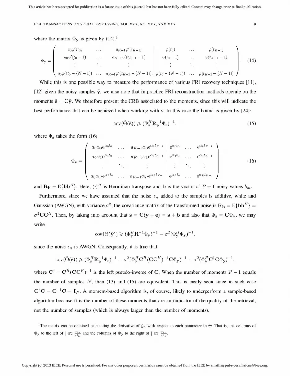
where the matrix Φy is given by (14).1

Φy �

��

a0ϕ1pt0q . . . aK�1ϕ

1ptK�1q ϕpt0q . . . ϕptK�1q

a0ϕ1pt0 � 1q . . . aK�1ϕ

1ptK�1 � 1q ϕpt0 � 1q . . . ϕptK�1 � 1q...

. . ....

.... . .

...

a0ϕ1pt0 � pN � 1qq . . . aK�1ϕ

1ptK�1 � pN � 1qq ϕpt0 � pN � 1qq . . . ϕptK�1 � pN � 1qq

�� . (14)

While this is one possible way to measure the performance of various FRI recovery techniques [11],

[12] given the noisy samples y, we also note that in practice FRI reconstruction methods operate on the

moments s � Cy. We therefore present the CRB associated to the moments, since this will indicate the

best performance that can be achieved when working with s. In this case the bound is given by [24]:

covpΘpsqq ¥ pΦHs R�1

b Φsq�1, (15)

where Φs takes the form (16)

Φs �

��

a0α0eα0t0 . . . aK�1α0eα0tK�1 eα0t0 . . . eα0tK�1

a0α1eα1t0 . . . aK�1α1eα1tK�1 eα1t0 . . . eα1tK�1

.... . .

......

. . ....

a0αP eαP t0 . . . aK�1αP eαP tK�1 eαP t0 . . . eαP tK�1

��

(16)

and Rb � EtbbHu. Here, p�qH is Hermitian transpose and b is the vector of P � 1 noisy values bm.

Furthermore, since we have assumed that the noise εn added to the samples is additive, white and

Gaussian (AWGN), with variance σ2, the covariance matrix of the transformed noise is Rb � EtbbHu �

σ2CCH . Then, by taking into account that s � Cpy � eq � s � b and also that Φs � CΦy, we may

write

covpΘpyqq ¥ pΦHy R�1Φyq

�1 � σ2pΦHy Φyq

�1,

since the noise εn is AWGN. Consequently, it is true that

covpΘpsqq ¥ pΦHs R�1

b Φsq�1 � σ2pΦH

y CHpCCHq�1CΦyq�1 � σ2pΦH

y C:CΦyq�1,

where C: � CHpCCHq�1 is the left pseudo-inverse of C. When the number of moments P � 1 equals

the number of samples N , then (13) and (15) are equivalent. This is easily seen since in such case

C:C � C�1C � IN . A moment-based algorithm is, of course, likely to underperform a sample-based

algorithm because it is the number of these moments that are an indicator of the quality of the retrieval,

not the number of samples (which is always larger than the number of moments).

1The matrix can be obtained calculating the derivative of yn with respect to each parameter in Θ. That is, the columns of

Φy to the left of | are BynBtk

and the columns of Φy to the right of | are BynBak

.




We have seen experimentally that FRI algorithms reach the bound (15) when C is sufficiently well

conditioned. Therefore our goal now is to design kernels that lead to properly conditioned C that

minimise (15) for any choice of P .2

IV. OPTIMAL EXPONENTIAL REPRODUCING KERNELS

As mentioned before, an exponential reproducing kernel can be written as ϕptq � γptq � β~αptq, where

γptq is arbitrary and β~αptq is an E-Spline. In this section we want to find rules on how to choose the

exponential parameters of the E-Spline αm � α � j πLp2m � P q for m � 0, . . . , P and the function

γptq in order to make FRI recovery techniques with these kernels as stable as possible. Finding the best

parameters translates into the optimisation of the matrix of coefficients C. Therefore we first determine

the properties that C has to satisfy and then design the kernels that lead to our choice of C.

A. How to choose matrix C

The first step in the FRI reconstruction stage is to transform the vector of samples y into the vector

of moments s � Cy, therefore, our first aim is to get a well conditioned C. From equation (12) we note

that matrix C is composed of elements cm,n � cm,0eαmn at position pm,nq, where n � 0, . . . , N � 1

and m � 0, . . . , P :

C �

��

c0,0 0 � � � 0

0 c1,0 � � � 0...

.... . .

...

0 0 � � � cP,0

��

loooooooooooooomoooooooooooooonD

��

1 eα0 � � � eα0pN�1q

1 eα1 � � � eα1pN�1q

......

. . ....

1 eαP � � � eαP pN�1q

��

loooooooooooooooomoooooooooooooooonV

.

Here, D is diagonal and V Vandermonde. Hence, to have a stable C we want the absolute values of the

diagonal elements of D to be the same, for instance |cm,0| � 1. Moreover, we want the elements in V

to lie on the unit circle:

eαmn � ejπ

Lp2m�P qn for m � 0, . . . , P , i.e. α � 0. (17)

Clearly, purely imaginary αm make the Vandermonde matrix V better conditioned [25]. We are

therefore only left with the problem of finding the best L in (17). Since we have experimentally seen

2The condition P � 1 � N can be imposed only for blockwise sampling, e.g. when sampling periodic signals using N

samples. This condition cannot be imposed on infinite length signals since sequential reconstruction algorithms will operate on

blocks with possibly varying number of samples.




that FRI algorithms are able to reach the CRB (15) if C is well conditioned, one way to determine L is

to choose the value that minimises (15) for the location of a single Dirac. It turns out the minimum is

always achieved when L � P �1, as shown in Figure 3 for various choices of P and L, given |cm,0| � 1

for all m.

1 1.5 2 2.5 3 3.5 4 4.5 5 5.5 60

0.005

0.01

0.015

0.02

0.025

0.03

0.035

0.04

0.045

0.05

L/(P+1)

s-CRB(t

0)

P+1=6P+1=11P+1=16P+1=21

Figure 3. CRB vs. L. Here we plot various CRB values (15) (σ � 1) for coefficients satisfying |cm,0| � 1, m � 0, . . . , P

when we vary L in equation (17). For any value of P the CRB is minimised when L � P � 1 (note that all the lines are

monotonically increasing).

To some extent, this is not surprising since this choice ensures that the exponentials span the entire

unit circle, which is well known to be the best configuration when recovering the parameters of a power

sum series [26]. Finally, when we impose P � 1 � N with L � P � 1, besides minimising (15), we also

ensure that the moment-based CRB in (15) matches the sample-based bound in (13), leading to the best

possible performance. In this situation, the matrix C ends up being square and unitary. This is the most

stable numerical transformation since its condition number is one.

In summary, the best exponential reproducing kernels should reproduce exponentials with exponents

of the form αm � j πP�1p2m � P q and have |cm,0| � 1 for m � 0, . . . , P . Finally, whenever possible,

the order of the kernel (which equals the number of moments) should be P � 1 � N . In the next section

we show how to obtain such kernels.

B. Exponential MOMS

Equipped with the analysis of the previous section, we now design optimal exponential reproducing

kernels of maximum-order and minimum-support (e-MOMS). We require |cm,0| � 1 for m � 0, . . . , P




and exponential parameters of the form:

αm � jωm � jπ

P � 1p2m� P q m � 0, . . . , P. (18)

By taking into account that any exponential reproducing kernel ϕptq can be written as ϕptq � γptq �

β~αptq, we design γptq so that |cm,0| � 1 is satisfied. We note that, by using (3), we have that

eαmt � cm,0¸nPZ

eαmnϕpt� nq.

Consequently

1 � cm,0¸nPZ

eαmpn�tqϕpt� nq

paq� cm,0

¸kPZ

ϕpαm � j2πkqej2πkt

pbq� cm,0ϕpαmq,

where paq follows from Poisson summation formula3 and pbq from the application of the generalised

Strang-Fix conditions (11). Therefore, we have that for any exponential reproducing kernel cm,0 �

ϕpαmq�1. We then realise that imposing |cm,0| � 1 is equivalent to requiring |ϕpαmq| � 1. Finally, by

using the fact that ϕpαmq � γpαmqβ~αpαmq and evaluating the Laplace transforms at αm � jωm, we

arrive at the following condition on γpjωmq:

|ϕpjωmq| � |γpjωmqβ~αpjωmq| � 1 Ø |γpjωmq| � |β~αpjωmq|�1, (19)

where we now work with the Fourier transform of each function.

Among all the admissible kernels satisfying (19), we are interested in the one with the shortest support

P � 1. We thus consider the kernels given by a linear combination of various derivatives of the original

E-Spline β~αptq, i.e.:

ϕptq �P

`�0

d`βp`q~α ptq, (20)

where βp`q~α ptq is the `th derivative of β~αptq, with βp0q~α ptq � β~αptq, and d` is a set of coefficients. This is

like saying that γptq is a linear combination of the Dirac delta and its derivatives, up to order P [23].

These kernels are still able to reproduce the exponentials eαmt and are a variation of the maximal-order

minimal-support (MOMS) kernels introduced in [27]. This is why we call them exponential MOMS (or

e-MOMS). They are also a specific case of the broader family of generalised E-Splines presented in [28].

3Poisson summation:¸nPZ

fpt� nT q �1

T

¸kPZ

f

�j

2πk

T

ej2πk

tT .




The advantage of this formulation is twofold: first the modified kernel ϕptq is of minimum support P �1,

the same as that of β~αptq; second we only need to find the coefficients d` that meet the constraint (19),

in order to achieve |cm,0| � 1. Using the Fourier transform of (20), which is given by:

ϕpjωq � β~αpjωqP

`�0

d`pjωq`,

we realise that we can satisfy (19) by choosing the coefficients d` so that the resulting polynomial

γpjωq �°` d`pjωq

` interpolates the set of points (jωm, |β~αpjωmq|�1q for m � 0, 1, . . . , P .

Once we have designed the kernels satisfying that cm,0 has modulus one for all m, we are left with

a phase ambiguity. Hypothesising a linear phase behavior, this ambiguity can be reduced to a time shift

∆ for the E-Spline in (20), introducing an additional degree of freedom. It is possible to show that, in

order for the exponential MOMS with |cm,0| � 1 and parameters (18) to be continuous-time functions,

then cm,0 � |cm,0|ejωm∆ for m � 0, . . . , P , where ∆ is an integer larger than or equal to 1 and smaller

than or equal to P .

In Figure 4 we present some of the kernels obtained by implementing the procedure explained above.

Interestingly, as shown in Appendix B, these specific functions always equal one period of the Dirichlet

kernel. We also point out that when P � 1 � N the scenario derived using this family of exponential

reproducing kernels converges to the original FRI formulation of [1] when we periodise the input or,

equivalently, the sampling kernel.

0 5 10 15 20 25 30

−0.2

0

0.2

0.4

0.6

0.8

1

t

(a) P � 1 � 6

0 5 10 15 20 25 30

−0.2

0

0.2

0.4

0.6

0.8

1

t

(b) P � 1 � 16

0 5 10 15 20 25 30

−0.2

0

0.2

0.4

0.6

0.8

1

t

(c) P � 1 � 31

Figure 4. Examples of exponential MOMS. These are 3 of the 30 possible kernels with support P � 1 ¤ N � 31 samples.

They coincide with one period of the Dirichlet kernel of period P � 1 for P even or 2pP � 1q for P odd (see Appendix B). All

of them are built selecting the phase of cm,0 such that they are continuous-time functions centred around ∆ � rP�12

s, where

r�s indicates rounded to the nearest integer. They are shown in the middle of the sampling interval for T � 1.




V. UNIVERSAL SAMPLING OF SIGNALS WITH FRI

In the previous section we have shown how to design optimal exponential reproducing kernels for noisy

FRI sampling. In many practical circumstances, however, the freedom to choose the sampling kernel ϕptq

is a luxury we may not have.

Essential in the FRI setting is the ability of ϕptq to reproduce exponential functions, because this allows

us to map the signal reconstruction problem to Prony’s method in spectral-line estimation theory. In this

section we relax this condition and consider any function ϕptq for which the exponential reproduction

property (3) does not necessarily hold. For these functions it is still possible to find coefficients cm,n such

that the reproduction of exponentials is approximate rather than exact. We propose to use this approximate

reproduction and the corresponding coefficients cm,n to retrieve FRI signals from the samples obtained

using these kernels.

This new approach has several advantages: First, it is universal in that it can be used with any kernel

ϕptq. In fact, as we shall show in the following sections, this new formulation does not even require an

exact knowledge of the kernel. Second, while reconstruction of FRI signals with this new method is not

going to be exact, we will show that in many cases a proper iterative algorithm can make the reconstruction

error arbitrarily small. Finally, it can be used to increase the resiliency to noise of some unstable kernels

proposed in the FRI literature. For example, kernels like polynomial splines or the Gaussian function

lead to very ill-conditioned reconstruction procedures. We show that by replacing the original C with the

one formed from properly chosen coefficients cm,n, based on approximate reproduction of exponentials,

we achieve a much more stable reconstruction with the same kernels.

A. Approximate reproduction of exponentials

Assume we want to use the linear combination of a function ϕptq and its integer shifts to approximate

the exponential eαt. Specifically, we want to find the coefficients cn such that:

¸nPZ

cnϕpt� nq u eαt. (21)

This approximation is exact only when ϕptq satisfies the generalised Strang-Fix conditions (11). For

any other function it is of particular interest to find the coefficients cn that best fit (21). In order to do




so, we directly use4 cn � c0eαn and introduce the 1-periodic function

gαptq � c0

¸nPZ

e�αpt�nqϕpt� nq. (22)

We then find that approximating the exponential eαt with integer shifts of ϕptq can be transformed

into approximating gαptq by the constant value 1. The reason is that we can rewrite (21) in the form of

the right-hand side of (22) by substituting cn � c0eαn and moving eαt to the left-hand side.

As a consequence of Poisson summation formula, we have that the Fourier series expansion of gαptq

is given by

gαptq �¸lPZgle

j2πlt �¸lPZc0ϕpα� j2πlqej2πlt

and that our approximation problem reduces to:

gαptq �¸lPZc0ϕpα� j2πlqej2πlt u 1. (23)

This shows more deeply the relation between the generalised Strang-Fix conditions (11) and the approx-

imation of exponentials. If ϕptq satisfies the generalised Strang-Fix conditions (11) then ϕpα�j2πlq � 0

for l P Zzt0u and (23) holds exactly when c0ϕpαq � 1. Otherwise, the terms ϕpα� j2πlq for l P Zzt0u

do not vanish, and we can only find the coefficient c0 so that gαptq u 1. However, the closer the values

ϕpα� j2πlq are to zero, the better the approximation in (21) is.

In general ϕptq can be any function and we can find different sets of coefficients cn in order for (21)

to hold. Regardless of the coefficients we use, we can determine the accuracy of our approximation by

using the Fourier series expansion of gαptq. In fact, the error of approximating fptq � eαt by the function

sptq �°nPZ cnϕpt� nq with coefficients cn � c0eαn is equal to:

εptq � fptq � sptq � eαt r1 � gαptqs (24)

� eαt

�1 � c0

¸lPZϕpα� j2πlqej2πlt

�.

Note that, if the Laplace transform of ϕptq decays sufficiently quickly, very few terms of the Fourier

series expansion are needed to have an accurate bound for the error.

A natural choice of the coefficients cn � c0eαn is the one given by the least-squares approximation.

Despite the fact that fptq is not square-integrable, we can still obtain the coefficients by computing the

4The exact exponential reproducing coefficients always satisfy cn � c0eαn. We now anticipate that different sets of

approximation coefficients we derive throughout the section also have the same form.




orthogonal projection of fptq onto the subspace spanned by ϕpt� nq [29]. They are

cn �ϕp�αq

aϕpeαqeαn,

where aϕpeαq �°lPZ aϕrlse

�αl is the z-transform of aϕrls � 〈ϕpt� lq, ϕptq〉, evaluated at z � eα.

The least-squares approximation has the disadvantage that it requires exact knowledge of ϕptq. How-

ever, as we stated before, if the Laplace transform of ϕptq decays sufficiently quickly, we can assume

the terms ϕpα � j2πlq are close to zero for l P Zzt0u. In this case we have that the error in (24) is

easily minimised by choosing c0 � ϕpαq�1. We denote this second type of approximation constant least-

squares. Besides its simplicity, a second advantage of choosing cn � ϕpαq�1eαn is that it requires only

the knowledge of the Laplace transform of ϕptq at α. If we put ourselves in the FRI setting where we

require the approximate reproduction of the exponentials eαmt with m � 0, . . . , P , then this simplified

formulation needs only the knowledge of the Laplace transform of ϕptq at αm, m � 0, . . . , P .

Finally, a third interesting choice of coefficients is the one that ensures that sptq interpolates fptq

exactly at integer points in time t � ` P Z [22], [30]. These coefficients are as follows:

cn �1°

lPZ e�αlϕplqeαn.

Note that in order to use the interpolation coefficients we only need information on ϕptq at integer instants

of time. We summarise the previous results in Table I.

Table I

COEFFICIENTS FOR THE APPROXIMATE REPRODUCTION (21)

Type Coefficients

Least-squares cn �ϕp�αq

aϕpeαqeαn

Constant least-squares cn � ϕpαq�1eαn

Interpolation cn �1°

lPZ e�αlϕplqeαn

According to our experience, in most cases, the constant least-squares approximation is just as good

as the least-squares approximation and has the advantage of requiring only the knowledge of the Laplace

transform of the kernel at s � α. Interpolation coefficients are also very easy to compute. However,




they always provide a worse approximation quality. Therefore, for the rest of the paper, we use constant

least-squares approximation and constant least-squares coefficients.

We show an example of the above analysis in Figure 5. Here we want to approximate exponentials using

linear combinations of integer shifts of a linear spline. First, note that this spline reproduces polynomials

of orders 0 and 1 exactly, as shown in Figure 5 (a-b). Then, with the same function, we approximately

reproduce 4 complex exponentials eαmt � ejπ

16p2m�7qt for m � 0, . . . , 3, using the constant least-squares

coefficients cm,n � ϕpαmq�1eαmn. We present the approximation of their real part in Figure 5 (c-f). We

notice that some exponentials are better approximated than others, in this example the ones with lower

frequency. If we used a higher order spline, the approximation quality would improve. However, we have

chosen a linear spline for illustration purposes. Also note that the number of exponentials that can be

approximated is now independent of the order of the spline.

0 1 2 3 4 5 6 70

0.2

0.4

0.6

0.8

1

t

(a) Reproduction of 1

0 1 2 3 4 5 6 70

1

2

3

4

5

6

7

t

(b) Reproduction of t

0 1 2 3 4 5 6 7

−1

−0.5

0

0.5

1

t

(c) Approximation of Rete�j7π16tu

0 1 2 3 4 5 6 7

−1

−0.8

−0.6

−0.4

−0.2

0

0.2

0.4

0.6

0.8

1

t

(d) Approximation of Rete�j5π16tu

0 1 2 3 4 5 6 7

−1

−0.8

−0.6

−0.4

−0.2

0

0.2

0.4

0.6

0.8

1

t

(e) Approximation of Rete�j3π16tu

0 1 2 3 4 5 6 7

0.2

0.3

0.4

0.5

0.6

0.7

0.8

0.9

1

1.1

t

(f) Approximation of Rete�jπ16tu

Figure 5. B-Spline kernel reproduction and approximation capabilities. Figures (a-b) show the exact reproduction of polynomials

of orders 0 and 1 with a linear spline. Figures (c-f) show the approximation of the real parts of 4 complex exponentials:

eαmt � ejπ16p2m�7qt for m � 0, . . . , 3, with the constant least-squares coefficients cm,n � ϕpαmq�1eαmn, using a linear

spline. We plot the weighted and shifted versions of the splines with dashed blue lines, the reconstructed polynomials and

exponentials with red solid lines, and the original functions to be reproduced with solid black lines.




B. Approximate FRI recovery

Consider again the stream of Diracs xptq �°K�1k�0 akδpt� tkq and the noiseless samples

yn �

⟨xptq, ϕ

�t

T� n

⟩�

K�1

k�0

akϕ

�tkT� n

. (25)

We want to retrieve the locations and amplitudes of the Diracs from the samples (25), but now we

make no assumption on the sampling kernel. We find proper coefficients for ϕptq to approximate the

exponentials eαmt, where m � 0, . . . , P , αm � α0 �mλ, and α0, λ P C. From the previous section we

know that a good approximation is achieved if we choose cm,n � cm,0eαmn with cm,0 � ϕpαmq�1. We

thus only need to know the Laplace transform of ϕptq at αm, m � 0, . . . , P . Also, note that P no longer

needs to be related to the support of ϕptq, but we can use any value subject to P � 1 ¥ 2K.

In order to retrieve the innovation parameters ttk, akuK�1k�0 , we proceed as in the case of exact repro-

duction of exponentials, but now using (24) we have that the moments are

sm �N�1

n�0

cm,nyn �

⟨xptq,

N�1

n�0

cm,nϕ

�t

T� n

loooooooooooomoooooooooooon

eαmtT �εmp tT q

⟩(26)

�K�1

k�0

xkumk �

K�1

k�0

akεm

�tkT

loooooooomoooooooon

ζm

where xk � akeα0

tkT and uk � eλ

tkT . There is a model mismatch due to the approximation error εmptq

of (24), equal to ζm. We treat it as noise and retrieve the parameters of the signal using the methods

of Section II-B. The model mismatch depends on the quality of the approximation, dictated by the

coefficients cm,n, the parameters αm and P , and the kernel ϕptq. The estimation of the Diracs can be

refined using the iterative algorithm shown in the box Algorithm 2. The basic idea of the algorithm is

that, given an estimate of the locations of the Diracs, we can compute an approximation of ζm and use

it to refine the computation of the moments sm. In noisy scenarios, if ζm is negligible when compared

to other forms of noise then the procedure is sufficiently good.

C. How to select the parameters αm

In Section IV we have determined that, if we have full control on the design of the sampling kernel,

we should use as many moments as samples: P � 1 � N , the exponential parameters should be purely

imaginary and of the form αm � j πP�1p2m�P q and the coefficients cm,n should be such that |cm,0| � 1




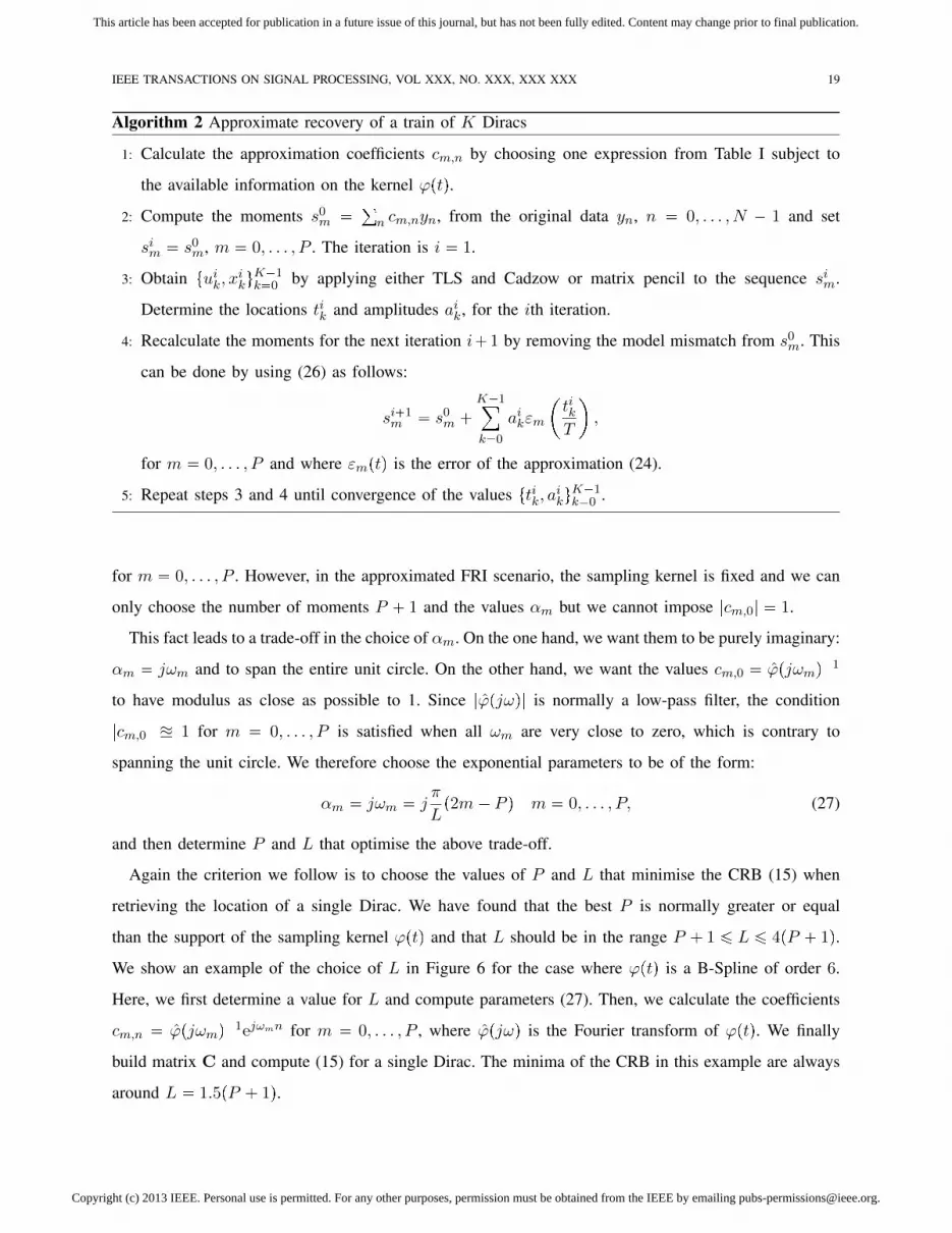
Algorithm 2 Approximate recovery of a train of K Diracs

1: Calculate the approximation coefficients cm,n by choosing one expression from Table I subject to

the available information on the kernel ϕptq.

2: Compute the moments s0m �

°n cm,nyn, from the original data yn, n � 0, . . . , N � 1 and set

sim � s0m, m � 0, . . . , P . The iteration is i � 1.

3: Obtain tuik, xikuK�1k�0 by applying either TLS and Cadzow or matrix pencil to the sequence sim.

Determine the locations tik and amplitudes aik, for the ith iteration.

4: Recalculate the moments for the next iteration i�1 by removing the model mismatch from s0m. This

can be done by using (26) as follows:

si�1m � s0

m �K�1

k�0

aikεm

�tikT

,

for m � 0, . . . , P and where εmptq is the error of the approximation (24).

5: Repeat steps 3 and 4 until convergence of the values ttik, aikuK�1k�0 .

for m � 0, . . . , P . However, in the approximated FRI scenario, the sampling kernel is fixed and we can

only choose the number of moments P � 1 and the values αm but we cannot impose |cm,0| � 1.

This fact leads to a trade-off in the choice of αm. On the one hand, we want them to be purely imaginary:

αm � jωm and to span the entire unit circle. On the other hand, we want the values cm,0 � ϕpjωmq�1

to have modulus as close as possible to 1. Since |ϕpjωq| is normally a low-pass filter, the condition

|cm,0| u 1 for m � 0, . . . , P is satisfied when all ωm are very close to zero, which is contrary to

spanning the unit circle. We therefore choose the exponential parameters to be of the form:


Lp2m� P q m � 0, . . . , P, (27)

and then determine P and L that optimise the above trade-off.

Again the criterion we follow is to choose the values of P and L that minimise the CRB (15) when

retrieving the location of a single Dirac. We have found that the best P is normally greater or equal

than the support of the sampling kernel ϕptq and that L should be in the range P � 1 ¤ L ¤ 4pP � 1q.

We show an example of the choice of L in Figure 6 for the case where ϕptq is a B-Spline of order 6.

Here, we first determine a value for L and compute parameters (27). Then, we calculate the coefficients

cm,n � ϕpjωmq�1ejωmn for m � 0, . . . , P , where ϕpjωq is the Fourier transform of ϕptq. We finally

build matrix C and compute (15) for a single Dirac. The minima of the CRB in this example are always

around L � 1.5pP � 1q.




1 1.5 2 2.5 3 3.5 4 4.5 5 5.5 60

0.01

0.02

0.03

0.04

0.05

0.06

L/(P+1)

s-CRB(t

0)

P+1=6P+1=11P+1=16P+1=21P+1=26y-CRB

Figure 6. CRB vs. L. Here we plot different CRB values (15) (σ � 1) for exponential parameters (27) when we vary L. We

use cm,n � ϕpωmq�1ejωmn for m � 0, . . . , P , where ϕpjωq is the Fourier transform of a B-Spline of order 6. Note that the

minima are always for L around L � 1.5pP � 1q.

VI. SIMULATIONS

We now present simulation results to validate the main contributions of the paper. Specifically, we

show the performance of the e-MOMS kernels introduced in Section IV-B and of the approximate FRI

recovery method introduced in Section V.

A. The experimental setup

We take N samples following the scheme of Figure 1 by directly calculating yn �°K�1k�0 akϕ

�tkT � n

�for n � 0, . . . , N � 1, since we have a train of K Diracs as the input. We then either use the noiseless

samples or corrupt them with additive white Gaussian noise of variance σ2. The variance is chosen

according to the target signal-to-noise ratio defined as SNRpdBq � 10 log }y}2

Nσ2 . We finally compute the

P � 1 noisy moments and then retrieve the innovation parameters tak, tkuK�1k�0 of the input using the

matrix pencil method.

We present results for single realisations of the sampling and reconstruction process or for average

performance over multiple trials. For the latter, we are mainly interested in the error in the estimation of

the time locations, since these are the most challenging parameters to retrieve. For each Dirac, we show

the standard deviation of this error:

∆tk �

d°I�1i�0 pt

piqk � tkq2

Ik � 0, . . . ,K � 1, (28)




where tpiqk are the estimated time locations at iteration i and I is the total number of iterations. We

calculate (28) for a range of fixed signal-to-noise ratios and average the effects using I � 1000 noise

realisations for each SNR. We compare the performance (28) with the square root of the variance predicted

by the two different Cramer–Rao bounds (CRB) of Section III: the sample-based CRB (13) and the

moment-based CRB (15).

B. Exponential MOMS

In Figure 7(a-b) we present simulation results when we retrieve K � 2 Diracs from N � 31

samples using a standard E-Spline and the exponential MOMS kernels of Section IV-B. The former are

characterised by purely imaginary exponents αm � j π2pP�1qp2m� P q for m � 0, . . . , P . The sampling

period is such that τ � NT � 1.

0 5 10 15 20 3010

−4

10−3

10−2

10−1

SNR

∆t/τ

e-MOMSe-MOMS y-CRBe-MOMS s-CRBE-Spline

(a) e-MOMS P � 1 � 16

0 5 10 15 20 3010

−4

10−3

10−2

10−1

SNR

∆t/τ

(b) e-MOMS P � 1 � 31

0 0.1 0.2 0.3 0.4 0.5 0.6 0.7 0.8 0.9 10

0.5

1

1.5

t

originalretrieved

(c) Retrieval of K � 20 Diracs

Figure 7. Performance of e-MOMS kernels. (a-b) compare the performance of e-MOMS and E-Splines of different orders

P � 1 when noise is added to N � 31 samples. We show the recovery of the first of K � 2 Diracs. Note that e-MOMS always

outperform E-splines and achieve the moment-based CRB (s-CRB). This bound gets closer to the sample-based CRB (y-CRB)

as the value of P � 1 increases and matches it when P � 1 � N . Finally, (c) shows the retrieval of K � 20 Diracs randomly

spaced over τ � NT � 1. The signal-to-noise ratio is 15dB, and we use N � 61 samples and P � 1 � N moments.

We see that for any order P � 1, e-MOMS outperform E-splines. Moreover, e-MOMS always achieve

the moment-based CRB (in red and denoted s-CRB in the legend). This bound gets closer to the sample-

based CRB (in black and denoted y-CRB in the legend) as the value of P � 1 increases and as expected

matches it when P � 1 � N .

To further illustrate the stability of e-MOMS, in Fig. 7(c) we show the retrieval of K � 20 Diracs

randomly spaced over τ � NT � 1 and with arbitrary amplitudes. We obtain N � 61 samples,

contaminate them with AWGN of signal-to-noise ratio equal to 15dB and estimate the Diracs from

P � 1 � N moments.




C. Approximate FRI Recovery

In this section we apply the approximate FRI sampling methods of Section V to two unstable kernels: B-

Splines and Gaussian kernel. We show that this new framework leads to much more precise reconstructions

than those obtained using the traditional exact FRI recovery methods.

1) The B-Spline case: In this example we compare the performance of our method with the traditional

recovery strategy based on the exact reproduction of polynomials [2]. We sample a stream of K � 6

Diracs that has been filtered with a B-Spline kernel of order M � 1 � 16. We then reconstruct the input

from N � 31 noisy samples by obtaining P � 1 moments using the constant least-squares coefficients.

These take the form cm,n � ϕpαmq�1eαmn, where ϕpsq represents the Laplace transform of the B-Spline.

We adjust L as suggested in Section V-C to choose appropriate exponential parameters αm � j πLp2m�P q,

m � 0, . . . , P . The Diracs are located at random over τ � NT � 1 and have arbitrary amplitudes. The

signal-to-noise ratio is SNR � 25dB.

In Figure 8(b) we present the estimation for the method based on reproduction of polynomials with

M � 1 � 16 moments. Note that not all the Diracs can be found. In Fig. 8(c) we show the estimation

given by the method based on approximation of exponentials, when we select L � 1.5pP � 1q and

generate P � 1 � 21 exponential moments. In this case all the Diracs are retrieved with a root mean

squared error on the estimation of the locations of the order of 10�3.

0 5 10 15 20 25 30

0

0.05

0.1

0.15

0.2

0.25

0.3

0.35

0.4

n

yn

yn

(a) yn and yn

0 0.1 0.2 0.3 0.4 0.5 0.6 0.7 0.8 0.9 10

0.2

0.4

0.6

0.8

1

1.2

t

originalretrieved

(b) Default FRI retrieval

0 0.1 0.2 0.3 0.4 0.5 0.6 0.7 0.8 0.9 10

0.2

0.4

0.6

0.8

1

1.2

t

originalretrieved

(c) Approximate FRI retrieval

Figure 8. Estimation of multiple Diracs with the B-Spline kernel. We recover K � 6 Diracs from (a) N � 31 noisy samples

taken by a kernel of order M �1 � 16. (b) Default polynomial recovery of [2], enhanced using pre-whitening. (c) Approximate

recovery with αm � j π1.5pP�1q

p2m� P q, m � 0, . . . , P where P � 1 � 21. The SNR in both cases is 25dB.

We show further results when we use the approximate method to retrieve K � 2 Diracs from N � 31

noisy samples taken by a B-Spline kernel of order M � 1 � 6. We use exponential parameters αm �

j πLp2m� P q with m � 0, . . . , P and L � 1.5pP � 1q. In Figure 9 we show that, even though the order




of the kernel is fixed at M � 1 � 6, we improve the performance by generating more moments, that

is, by choosing P ¡ M . As the number of moments increases, the performance improves to eventually

reach the sample-based CRB as shown in Fig. 9(c).

0 5 10 15 20 3010

−4

10−3

10−2

10−1

SNR

∆t/τ

FRIy-CRBs-CRB

(a) P � 1 � 6

0 5 10 15 20 3010

−4

10−3

10−2

10−1

SNR

∆t/τ

(b) P � 1 � 16

0 5 10 15 20 3010

−4

10−3

10−2

10−1

SNR

∆t/τ

(c) P � 1 � 26

Figure 9. Approximate retrieval using a B-Spline. These figures show the error in the estimation of the first Dirac out of

K � 2 retrieved using the approximated FRI recovery. We show how, even when we fix the order of the kernel P � 1, we can

reconstruct any number of moments P � 1 and improve the performance. In fact, with the appropriate choice L � 1.5pP � 1q

the performance improves until the sample-based CRB is reached.

2) The Gaussian kernel case: We conclude this set of simulations by showing an example with the

Gaussian kernel hγptq � e�t2{p2γ2q [1]. Since for this kernel the samples are yn � 〈xptq, hγpnT � tq〉

the approximation problem (21) becomes:

eα1t �

¸nPZ

cnhγpt� nT q.

In order to use the coefficients of Table I we need to consider α1 � αT and ϕptq � hγpTtq and manipulate

the original expressions. For example, the constant least-squares coefficients are now given by cm,n �

T hγpα1mq

�1eα1mnT . Here, again α1m � j πLp2m � P q, m � 0, . . . , P and we adjust L as suggested in

Section V-C.

In Figure 10 we show the reconstruction of K � 5 Diracs from N � 61 noisy samples taken by a

Gaussian kernel of standard deviation γ � 0.09677 with sampling period T � 131 . The signal-to-noise

ratio is SNR � 25dB. We choose L � 3.5T pP � 1q to compute the constant least-squares coefficients

and generate P � 1 � 21 moments to estimate the parameters of the Diracs. The Diracs have random

locations in the interval r0, 1.2s. Fig. 10(b) shows that all the Diracs are correctly retrieved with a root

mean squared error on the estimation of the locations of the order of 3 � 10�3. We also note that this

kernel is so unstable that the traditional FRI exact recovery method of [11] fails completely in this case.




0 10 20 30 40 50 60

0

0.5

1

1.5

n

yn

yn

(a) yn and yn

0 0.2 0.4 0.6 0.8 1 1.2 1.4 1.6 1.8 20

0.5

1

1.5

t

originalretrieved

(b) Approximate FRI retrieval

Figure 10. Approximate FRI with the Gaussian kernel. We recover K � 5 Diracs from (a) N � 61 noisy samples taken by

a Gaussian kernel of standard deviation γ � 0.09677 with period T � 131

. (b) Recovery using the approximate method with

αm � j π3.5T pP�1q

p2m� P q, m � 0, . . . , P where P � 1 � 21. The SNR is 25dB.

D. Approximation error and accuracy of the reconstruction

In this example we test the hypothesis that better approximation of exponentials leads to more accurate

reconstruction of Diracs. Assume we sample a single Dirac with a linear spline and we recover its location

using approximation of exponentials. In Figure 5 we have shown that the linear spline can approximate

complex exponentials of lower frequencies better than those with higher frequencies. We now generate

four moments sm using the constant least-squares coefficients that are associated to the same exponentials

eαmt � ejπ

16p2m�7qt for m � 0, . . . , 3 of Figure 5. Finally, we compare the estimation of the location

of the Dirac obtained from the moments associated to the higher frequencies (HF) s0 and s1 to the

estimation obtained from the moments associated to the lower frequencies (LF) s2 and s3.

In Table II we show the root mean squared error of the estimation obtained from either pair of

moments. The error is averaged over 100 realisations each of which corresponds to placing the Dirac

at t0 � 0.15pi� 1q for i � 1, . . . , 100. As expected the approximation with lower frequency achieves a

better performance.

Table II

ACCURACY OF THE RECONSTRUCTION

HF LF

s0 s1 s2 s3

Approximation error 0.061 0.028 0.0093 0.00098

Reconstruction error 0.0018 0.00019




E. Alternative FRI signals

We conclude the simulations by showing that it is possible to adapt the approximate FRI framework to

sample and reconstruct alternative FRI signals. For example, sampling a piecewise constant function with

a kernel ϕptq and calculating the first finite difference of the samples zn � yn � yn�1 yields the same

measurements as sampling the derivative of the signal with φptq � ϕptq � β0ptq, where β0ptq is a box

function [2]. The derivative of the signal is a train of K Diracs. Consequently, we may recover the signal

by calculating cm,n for the linear combination of shifted versions of φptq to approximate exponentials

and then applying the annihilating filter method to the moments sm �°n cm,nzn.

We illustrate the process in Figure 11. Here, we sample a piecewise constant function with K � 6

discontinuities using a B-Spline kernel of order M�1 � 6. The sampling period is T � 115 . In Fig. 11(a)

we show the N � 32 samples contaminated with additive white Gaussian noise and in Fig. 11(b) we

show their first order difference. Then, we generate P �1 � 21 moments using the constant least-squares

coefficients from exponential parameters αm � j πLp2m � P q with m � 0, . . . , P and L � 1.4pP � 1q.

The signal-to-noise ratio is 25dB. Note that the order of the spline is not sufficient to apply the retrieval

method based on reproduction of polynomials of [2]. On the contrary, we can use the method based on

approximation of exponentials as long as P � 1 ¥ 2K. The original and reconstructed signal are shown

in Fig. 11(c).

0 5 10 15 20 25 30

−0.5

0

0.5

1

1.5

2

2.5

3

3.5

n

yn

yn

(a) Samples

0 5 10 15 20 25 30

−1

−0.5

0

0.5

1

1.5

2

n

zn

zn

(b) Equivalent samples

0 0.2 0.4 0.6 0.8 1 1.2 1.4 1.6 1.8 2

−0.5

0

0.5

1

1.5

2

2.5

3

3.5

t

originalretrieved

(c) Retrieved signal

Figure 11. Piecewise constant functions and B-Splines. These figures show the sampling and retrieval process, based on

approximation of exponentials, for a piecewise constant function with K � 6 discontinuities in the presence of noise of 25dB.

VII. CONCLUSIONS

In this paper we have considered the FRI reconstruction problem in the presence of noise. We have

first revisited existing results in the noiseless setting, and the most effective treatment of noise in the




current literature. Then, we have studied robust alternatives to the previous line of work.

More specifically, our contribution is twofold: We have determined how to design optimal exponential

reproducing kernels, in the sense that they lead to the most stable signal reconstruction. Moreover, we

have departed from the ideal situation in which we have full control of the sampling kernel and considered

the case where we are given corrupted samples taken with an arbitrary acquisition device. In this situation,

we have developed a universal FRI reconstruction strategy that works with any kernel. In contrast to the

original FRI framework, which tries to find the exact parameters of the input signal, we have proposed an

approximate recovery of the input based on the approximate reproduction of exponentials. The advantage

of our new approach is that it can be applied to any sampling kernel and provides more stable and precise

reconstructions than those obtained with specific classes of kernels used in the past.

APPENDIX A

GENERALISED STRANG-FIX CONDITIONS

An exponential reproducing kernel is any function ϕptq that, together with a linear combination of its

shifted versions, can generate exponential polynomials of the form treαmt [22], [28] for m � 0, . . . , P

and r � 0, . . . , R. The parameters αm are in general complex. In this appendix we prove that exponential

reproducing kernels satisfy the generalised Strang-Fix conditions. More specifically, a kernel ϕptq is able

to reproduce exponential polynomials, i.e.:

treαmt �¸nPZ

cm,n,rϕpt� nq,

if and only if

ϕprqpαmq � 0 and ϕprqpαm � j2πlq � 0

for l � 0, r � 0, . . . , R and m � 0, . . . , P . Here, ϕprqpsq represents the rth order derivative of the

double-sided Laplace transform of ϕptq.

The proof is obtained from the Strang-Fix conditions for polynomial reproducing kernels, by consider-

ing the function ψptq � e�αmtϕptq that clearly reproduces polynomials of the form tr for r � 0, . . . , R.

The Strang-Fix conditions [2], [31] state that a kernel ψptq is able to reproduce polynomials, i.e.:

tr �¸nPZ

cr,nψpt� nq,

if and only if

ψp0q � 0 and ψprqpj2πlq � 0




for l � 0 and r � 0, . . . , R. Here, ψpjωq is the Fourier transform of ψptq, and ψprqpjωq represents its

rth order derivative. Then, by taking into account that the Fourier transform of ψptq is related to the

Laplace transform of ϕptq through ψpjωq � ϕpαm � jωq, the above equation turns into the generalised

Strang-Fix conditions for ϕptq:

ϕpαmq � 0 and ϕprqpαm � j2πlq � 0

for l � 0, r � 0, . . . , R and m � 0, . . . , P . Now ϕprqpsq represents the rth order derivative of the

double-sided Laplace transform of ϕptq. This proves that a kernel that reproduces exponential polynomials

satisfies the generalised Strang-Fix conditions.

The converse is also true. Consider a kernel ϕptq that satisfies the generalised Strang-Fix conditions.

Then, a kernel ψptq with Fourier transform ψpjωq � ϕpαm� jωq is guaranteed to satisfy the Strang-Fix

conditions and, consequently, reproduces polynomials tr for r � 0, . . . , R. Finally, due to the relation

of the kernels in the Laplace domain it follows that ψptq � e�αmtϕptq implying that ϕptq reproduces

exponential polynomials treαmt for l � 0, r � 0, . . . , R and m � 0, . . . , P , which completes the proof.

APPENDIX B

E-MOMS INCLUDE THE DIRICHLET AND SOS KERNELS

Let us consider the exponential reproducing kernel ϕ0ptq � ϕ�t� P�1

2

�of support P �1 and centred

in zero, with ϕptq � γptq � β~αptq, where β~αptq is an E-Spline. We restrict our analysis to P being even

and we use exponential parameters


P � 1p2m� P q, (29)

where m � 0, . . . , P . We next use the P �1–periodic extension of ϕ0ptq, that is ϕP�1ptq �°lPZ ϕ0pt�

lpP � 1qq, which is equivalent to:

ϕP�1ptq �1

P � 1

¸kPZ

ϕ0

�j

2πk

P � 1

ej

2πk

P�1t, (30)

from the application of Poisson summation formula. The case of P being odd can be derived likewise,

but by periodising over 2pP �1q. Also note that the Fourier transform of the shifted kernel ϕ0ptq is equal

to:

ϕ0pjωq � γpjωqP¹

m�0

sinc

�ω � ωm

2

. (31)

The set of equations

ϕ0pjωmq � |ϕpjωmq| � |γpjωmqβ~αpjωmq| � ηm, (32)




are just like (19) and lead to design exponential reproducing kernels of maximum order and minimum

support (e-MOMS), different from those of Section IV-B, but that still correspond to a specific subfamily

of the generalised exponential reproducing kernels of [28].

In (30) the Fourier transform ϕ0pjωq is evaluated at jωk � j 2πkP�1 . Taking into account (32), we know

that ϕ0pjωkq � ηk for k � �P2 , . . . ,

P2 . We also have that ϕ0pjωkq � 0 for any other k, because we can

find a term in the product (31) equal to sincp`πq � 0, ` P Z. Therefore, (30) can be reduced to:

ϕP�1ptq �1

P � 1

P

2

k��P

2

ηkej 2πk

P�1t. (33)

Note that when the values ηk � 1 for all k, then (33) reduces to one period of the Dirichlet kernel of

period P � 1:

ϕP�1ptq �1

P � 1

P

2

k��P

2

ej2πk

P�1t �

1

P � 1

sinpπtq

sinp πtP�1q

.

And this is precisely the P � 1–periodic extension of the e-MOMS kernels of Section IV-B.

To end, we now consider one period of (33) and denote t � xT , N � P � 1 and τ � NT � pP � 1qT .

Then we get the time domain definition of the SoS kernel [3]:

ϕP�1

� xT

� gpxq � rect

�xτ

1

N

¸kPK

ηkej 2πk

τx.

Here, the number of samples N needs to be odd, since P is even, and the set of indices K � t�N�12 , . . . , N�1

2 u.

REFERENCES

[1] M. Vetterli, P. Marziliano, and T. Blu, “Sampling signals with finite rate of innovation,” IEEE Transactions on Signal

Processing, vol. 50, pp. 1417–1428, June 2002.

[2] P. L. Dragotti, M. Vetterli, and T. Blu, “Sampling Moments and Reconstructing Signals of Finite Rate of Innovation:

Shannon Meets Strang-Fix,” IEEE Transactions on Signal Processing, vol. 55, pp. 1741–1757, May 2007.

[3] R. Tur, Y. C. Eldar, and Z. Friedman, “Innovation Rate Sampling of Pulse Streams with Application to Ultrasound Imaging,”

IEEE Transactions on Signal Processing, vol. 59, pp. 1827–1842, April 2011.

[4] P. Stoica and R. L. Moses, Introduction to Spectral Analysis. Englewood Cliffs, NJ: Prentice-Hall, 2000.

[5] A. Hormati and M. Vetterli, “Compressive Sampling of Multiple Sparse Signals Having Common Support Using Finite

Rate of Innovation Principles,” IEEE Signal Processing Letters, vol. 18, pp. 331–334, May 2011.

[6] J. Berent, P. L. Dragotti, and T. Blu, “Sampling Piecewise Sinusoidal Signals With Finite Rate of Innovation Methods,”

IEEE Transactions on Signal Processing, vol. 58, pp. 613–625, February 2010.

[7] I. Maravic and M. Vetterli, “Exact Sampling Results for Some Classes of Parametric Non-Bandlimited 2-D Signals,” IEEE

Transactions on Signal Processing, vol. 52, pp. 175–189, January 2004.

[8] P. Shukla and P. L. Dragotti, “Sampling Schemes for Multidimensional Signals with Finite Rate of Innovation,” IEEE

Transactions on Signal Processing, vol. 55, pp. 3670–3686, July 2007.




[9] H. Pan, T. Blu, and P. L. Dragotti, “Sampling Curves with Finite Rate of Innovation,” Proceedings of the Ninth International

Workshop on Sampling Theory and Applications (SampTA’11), Singapore, May 2011.

[10] C. Chen, P. Marziliano, and A. C. Kot, “2D Finite Rate of Innovation Reconstruction Method for Step Edge and Polygon

Signals in the Presence of Noise ,” IEEE Transactions on Signal Processing, vol. 60, pp. 2851–2859, June 2012.

[11] I. Maravic and M. Vetterli, “Sampling and reconstruction of signals with finite rate of innovation in the presence of noise,”

IEEE Transactions on Signal Processing, vol. 53, pp. 2788–2805, August 2005.

[12] T. Blu, P. L. Dragotti, M. Vetterli, P. Marziliano, and L. Coulot, “Sparse Sampling of Signal Innovations,” IEEE Signal

Processing Magazine, vol. 25, no. 2, pp. 31–40, 2008.

[13] V. Y. F. Tan and V. K. Goyal, “Estimating signals with finite rate of innovation from noisy samples: A stochastic algorithm,”

IEEE Transactions on Signal Processing, vol. 56, pp. 5135–5146, October 2008.

[14] A. Erdozain and P. M. Crespo, “A new stochastic algorithm inspired on genetic algorithms to estimate signals with finite

rate of innovation from noisy samples,” Signal Processing, vol. 90, pp. 134–144, January 2010.

[15] A. Erdozain and P. M. Crespo, “Reconstruction of aperiodic FRI signals and estimation of the rate of innovation based on

the state space method,” Signal Processing, vol. 91, no. 8, pp. 1709–1718, 2011.

[16] J. A. Uriguen, P. L. Dragotti, and T. Blu, “On the exponential reproducing kernels for sampling signals with finite rate

of innovation,” Proceedings of the Ninth International Workshop on Sampling Theory and Applications (SampTA’11),

Singapore, May 2011.

[17] I. Khalidov, T. Blu, and M. Unser, “Generalized L-Spline Wavelet Bases,” in Proceedings of the SPIE Conference on

Mathematical Imaging: Wavelet XI, vol. 5914, (San Diego CA, USA), pp. 59140F–1–59140F–8, July 31-August 3, 2005.

[18] J. A. Cadzow, “Signal Enhancement – A Composite Property Mapping Algorithm,” IEEE Transactions on Acoustics, Speech

and Signal Processing, vol. 36, pp. 49–62, January 1988.

[19] Y. Hua and T. K. Sakar, “Matrix Pencil Method for Estimating Parameters of Exponentially Damped Undamped Sinusoids

in Noise,” IEEE Transactions on Acoustics, Speech and Signal Processing, vol. 38, pp. 814–824, May 1990.

[20] B. D. Rao, “Model based processing of signals: A state space approach,” Proceedings of the IEEE, vol. 3980, pp. 283–309,

February 1992.

[21] Y. C. Eldar and A. V. Oppenheim, “MMSE Whitening and Subspace Whitening,” IEEE Transactions on Signal Processing,

vol. 49, pp. 1846–1851, July 2003.

[22] M. Unser and T. Blu, “Cardinal Exponential Splines: Part I—Theory and Filtering Algorithms,” IEEE Transactions on

Signal Processing, vol. 53, pp. 1425–1438, April 2005.

[23] A. Ron, “Factorization theorems for univariate splines on regular grids,” Israel Journal of Mathematics, vol. 70, no. 1,

pp. 48–68, 1990.

[24] E. Ollila, “On the Cramer-Rao bound for the constrained and unconstrained complex parameters,” Sensor Array and

Multichannel Signal Processing Workshop, pp. 414–418, July 2008.

[25] L. Berman and A. Feuer, “On perfect conditioning of vandermonde matrices on the unit circle,” Electronic Journal of

Linear Algebra, vol. 16, pp. 157–161, July 2007.

[26] G. H. Golub, P. Milanfar, and J. Varah, “A stable numerical method for inverting shape from moments,” SIAM Journal on

Scientific Computing (SISC), vol. 21, pp. 1222–1243, December 1999.

[27] T. Blu, P. Thevenaz, and M. Unser, “MOMS: maximal-order interpolation of minimal support,” IEEE Transactions on

Image Processing, vol. 10, pp. 1069–1080, July 2001.




[28] M. Unser, “Cardinal Exponential Splines: Part II—Think Analog, Act Digital,” IEEE Transactions on Signal Processing,

vol. 53, pp. 1439–1449, April 2005.

[29] M. Unser, A. Aldroubi, and M. Eden, “Polynomial Spline Signal Approximations: Filter Design and Asymptotic Equivalence

with Shannon’s Sampling Theorem,” IEEE Transactions on Information Theory, vol. 38, pp. 95–103, January 1992.

[30] M. Unser, “Sampling-50 years after Shannon,” in Proceedings of the IEEE, pp. 569–587, April 2000.

[31] G. Strang and G. Fix, “Fourier analysis of the finite element variational method,” Constructive Aspect of Functional

Analysis, pp. 796–830, 1971.

Jose Antonio Uriguen received the “Tıtluo de Ingeniero de Telecomunicaciones” from the “Universidad

del Paıs Vasco”, Spain, in 2000 (third out of 100 students); the M.S. degree in Communications and

Signal Processing from Imperial College (with Distinction), London, in 2009; and the Ph.D. degree from

Imperial College, London, in 2013.

He was one of the 120 recipients of a scholarship by the “Fundacion Caja Madrid”, awarded for

academic merits, to complete the first two years of his Ph.D. He was then supported by the RecoSamp

project and during this period developed advances in sampling theory for which he has one patent pending.

He is currently a research assistant with the University of Deusto, Spain. His research interests include applied mathematics,

interpolation, approximation and sampling theory, sparse sampling and biomedical signal processing.

Thierry Blu (F’12) was born in Orleans, France, in 1964. He received the “Diplome d’ingenieur” from

Ecole Polytechnique, France, in 1986 and from Telecom Paris (ENST), France, in 1988, and the Ph.D.

degree in electrical engineering from ENST in 1996 for a study on iterated rational filterbanks, applied

to wideband audio coding.

Between 1998 and 2007, he was with the Biomedical Imaging Group at the Swiss Federal Institute

of Technology (EPFL) in Lausanne, Switzerland. He is now a Professor in the Department of Electronic

Engineering, The Chinese University of Hong Kong.

Dr. Blu was the recipient of two best paper awards from the IEEE Signal Processing Society (2003 and 2006). He is also

coauthor of a paper that received a Young Author best paper award (2009) from the same society. He has been an Associate

Editor for the IEEE TRANSACTIONS ON IMAGE PROCESSING (2002-2006), the IEEE TRANSACTIONS ON SIGNAL PROCESSING

(2006-2010), Elsevier Signal Processing (2008-2011). He is currently on the board of Eurasip J. on Image and Video Processing

(since 2010) and is a member of the IEEE Signal Processing Theory and Methods Technical Committee (since 2008).

Research interests: (multi)wavelets, multiresolution analysis, multirate filterbanks, interpolation, approximation and sampling

theory, sparse sampling, image denoising, psychoacoustics, biomedical imaging, optics, wave propagation




Pier Luigi Dragotti is currently a Reader (Associate Professor) with the Electrical and Electronic

Engineering Department, Imperial College London, London, U.K.

He received the Laurea degree (summa cum laude) in electrical engineering from the University of

Naples Federico II, Naples, Italy, in 1997; the master’s degree in communications systems from the Swiss

Federal Institute of Technology of Lausanne (EPFL), Lausanne, Switzerland, in 1998, and the Ph.D. degree

from EPFL in April 2002. He has held several visiting positions at different universities and research

centers. He was a Visiting Student with Stanford University, Stanford, CA, USA, 1996, a Researcher with the Mathematics

of Communications Department, Bell Labs, Lucent Technologies, Murray Hill, NJ, USA, 2000, a Visiting Professor with the

Politecnico of Milan, Milan, Italy, 2010, and a Visiting Scientist with the Massachusetts Institute of Technology, Cambridge,

MA, USA, 2011.

He was a Technical Co-Chair for the European Signal Processing Conference in 2012, an Associate Editor of the IEEE

TRANSACTIONS ON IMAGE PROCESSING from 2006 to 2009 and an Elected Member of the IEEE Image, Video and Multidi-

mensional Signal Processing Technical Committee and the IEEE Signal Processing Theory and Methods Technical Committee.

He is a recipient of the ERC Starting Investigator Award for the project RecoSamp. His work includes sampling theory,

wavelet theory and its applications, image and video compression, image-based rendering, and image super-resolution. He has

published more than 100 publications and a patent acquired by Qualcomm, Inc., in 2007.

Documents

FRI Sampling With Arbitrary Kernels