HUSCAP: Hokkaido University Collection of Scholarly and Academic Papers

Title Integrated kernels and their properties

Author(s)Tanaka, Akira; Imai, Hideyuki; Kudo, Mineichi;

Miyakoshi, Masaaki

Citation Pattern Recognition, 40(11): 2930-2938

Issue Date 2007-11

Type article (author version)

URL http://hdl.handle.net/2115/30166

Right

Integrated Kernels and Their Properties

Akira Tanaka, Hideyuki Imai, Mineichi Kudo, and Masaaki MiyakoshiDivision of Computer Science,

Graduate School of Information Science and Technology,Hokkaido University, N14W9, Kita-ku, Sapporo 060-0814, Japan.

abstractKernel machines are widely considered to be powerful tools in various fields

of information science. By using a kernel, an unknown target is represented bya function that belongs to a reproducing kernel Hilbert space (RKHS) corre-sponding to the kernel. The application area is widened by enlarging the RKHSsuch that it includes a wide class of functions. In this study, we demonstrate amethod to perform this by using parameter integration of a parameterized ker-nel. Some numerical experiments show that the unresolved problem of findinga good parameter can be neglected.

keywordkernel, reproducing kernel Hilbert space, projection learning, parameter in-

tegration

1 Introduction

Learning based on kernel machines [1, 2, 3] has been widely considered to be apowerful tool in various fields of information science such as pattern recognition,regression estimation, density estimation, etc. In several existing approaches,the adequacy of kernel machines is measured by the difference between thepredictive output of an assumed model with the training input data set anda training output data set (e.g., class labels in a pattern recognition problem,function values in a density or regression estimation problem, etc.). In theseapproaches, a kernel, whose mathematical properties are described in detail in[4], is recognized as a useful tool for calculating the inner product in a certainfeature space.

On the other hand, Ogawa formulated a learning problem as an estimationof the unknown function in a certain function space. In this approach, theadequacy of learning is measured by the difference between the unknown truefunction and the estimated one in the function space determined by a kernel.Therefore, a kernel plays a crucial role in the determination of a function spaceto which the unknown target function belongs. This scheme is referred to as

1

(parametric) projection learning [5, 6, 7, 8] and it has been yielding severalinteresting results, primarily in the field of neural networks (see [9] for instance).This approach seems reasonable since it is widely known that the mathematicalessence of using a kernel is that the unknown target (a classifier in a patternrecognition problem, function in a density or regression estimation problem,etc.) can be represented by a function that belongs to a reproducing kernelHilbert space (RKHS) [4] that corresponds to an adopted kernel.

In the real world, however, targets to be learned are not always functionsas one found in a pattern recognition problem in which some classes essentiallyoverlap. The application of kernel machines to such problems requires meth-ods such as the “soft margin” technique in a support vector machine (SVM)[10]. On the other hand, it is also important to analyze the performance andproperties of a kernel machine when the unknown target can be represented bya function. In such a case, the use of kernel is theoretically validated. Here,one of the primary topics that requires theoretical clarification is the question:What constitutes a good kernel? As already mentioned, the condition thatthe unknown true function belongs to the RKHS corresponding to an adoptedkernel imparts theoretical consistency to kernel machines. This understandingprovides a suggestion for designing a kernel. In general, information about theunknown true function is limited. Therefore, we have to construct the RKHS tobe as large as possible. This imparts consistency to kernel machines for a wideclass of functions. In this study, we show that a kernel corresponding to such alarge RKHS is realized by the parameter integration of a parameterized kernel.Further, some numerical examples are given in order to validate our theory.

2 Mathematical Preliminaries for the RKHS The-ory

In this section, we prepare some mathematical tools to deal with the RKHStheory.

Definition 1 [4] Let Rn be an n-dimensional real vector space and let H bea class of functions defined on D ⊂ Rn, forming a Hilbert space of real-valuedfunctions. The function K(x, y) (x, y ∈ D) is referred to as a reproducingkernel of H, if

1. for every y ∈ D, K(x, y) is a function of x belonging to H and

2. for every y ∈ D and every f ∈ H,

f(y) = 〈f(x), K(x,y)〉, (1)

where 〈·, ·〉 denotes the inner product of the Hilbert space H.

The Hilbert space H is referred to as an RKHS when it has a reproducingkernel. The reproducing property, Eq.(1), enables the realization of the value

2

of the function at a point in D. Note that the reproducing kernels are positivedefinite [4]:

N∑i,j=1

cicjK(xi,xj) ≥ 0, (2)

for any N , c1, . . . , cN ∈ R, and x1, . . . , xN ∈ D. In addition, K(x, y) =K(y,x) for any x, y ∈ D follows [4]. If a reproducing kernel K(x, y) exists, itis unique [4]. Conversely, every positive definite function K(x, y) has a uniquecorresponding RKHS [4]. Therefore, it is guaranteed that any positive definitefunction K(x, y) is always a reproducing kernel.

Next, we introduce the Schatten product [11] that distinctly reveals thereproducing property of kernels.

Definition 2 [11] Let H1 and H2 be Hilbert spaces. The Schatten product ofg ∈ H2 and h ∈ H1 is defined as

(g ⊗ h)f := 〈f, h〉g, f ∈ H1. (3)

Note that (g ⊗ h) is a linear operator from H1 onto H2. It can be easilyshown that the following relations hold for h, v ∈ H1 and g, u ∈ H2:

(h ⊗ g)∗ = (g ⊗ h), (h ⊗ g)(u ⊗ v) = 〈u, g〉(h ⊗ v), (4)

where X∗ denotes the adjoint operator of X.

3 Interpretation of Learning as a Linear InverseProblem

Let (yi, xi), (yi ∈ R, xi ∈ Rn, i = 1, . . . , `) be a given training data set of `samples that satisfies

yi = f(xi) + ni, (5)

where f and ni ∈ R denote a real-valued function and additive noise, respec-tively. In regression estimation or density estimation problems, yi takes a realvalue, whereas yi takes a class label in pattern recognition problems. In thisstudy, the aim of the machine learning is assumed to be the estimation of theunknown function f using a training data set, a priori knowledge about thefunction space, and statistical properties of additive noise. In this study, weassume that f belongs to HK , the RKHS corresponding to a certain kernel K.Based on the reproducing property of kernels, the value of a function f ∈ HK

at a point xi is written as

f(xi) = 〈f(x),K(x, xi)〉. (6)

Therefore, Eq.(5) is rewritten as

yi = 〈f(x),K(x,xi)〉 + ni. (7)

3

Let y := [y1, . . . , y`]′ and n := [n1, . . . , n`]′, where X ′ denotes the transposedmatrix (or vector) of X. By applying the Schatten product to Eq.(7), we have

y =

(∑̀k=1

[e(`)k ⊗ K(x,xk)]

)f(x) + n, (8)

where e(`)k denotes the k-th vector of the canonical basis of R`. For simplicity,

we use

A :=

(∑̀k=1

[e(`)k ⊗ K(x, xk)]

). (9)

It is important to note that operator A is linear, irrespective of whether f(x)sare linear or non-linear. Now, the simplest form of Eq.(8) can be expressed as

y = Af(x) + n. (10)

This equation represents the relation between the unknown target function f(x)and output y. All the information about the input vectors is integrated inoperator A. Therefore, a machine learning problem can be interpreted as aninverse problem of Eq.(10) [5, 6].

Based on the model described by Eq.(10), Ogawa proposed a novel learn-ing framework referred to as (parametric) projection learning [5, 6]. Projectionlearning yields a minimum variance unbiased estimator of the orthogonal pro-jection of the unknown function f(x) onto R(A∗), the range of A∗; on the otherhand, parametric projection learning results in an improvement in the unknownfunction by incorporating the relaxation of the unbiasedness of projection learn-ing to suppress the influence of noise. Parametric projection learning includesprojection learning as a special case. In the framework of (parametric) projec-tion learning, the solution is the learning operator B; by using it, the estimatedfunction is expressed as

f̂(x) = By. (11)

Parametric projection learning is defined as follows:

Definition 3 [7, 8] The learning operator BPPL of parametric projection learn-ing is given as

BPPL(γ) := argminB [tr[(BA − PR(A∗))(BA − PR(A∗))∗]+ γEn||Bn||2], (12)

where PR(A∗) denotes the orthogonal projector onto R(A∗) and γ denotes a realpositive parameter that controls the trade-off between the two terms.

As shown in [7, 8], one of the solutions of the parametric projection learningis given as

BPPL(γ) = A∗(AA∗ + γQ)+, (13)

4

where X+ denotes the Moore-Penrose generalized inverse [12] of X, and Qdenotes the noise correlation operator defined by

Q := En[nn∗]. (14)

Finally, the solution of the parametric projection learning is written as

f̂(x) = BPPLy, (15)

or specifically

f̂(x) =

(∑̀i=1

[K(x, xi) ⊗ e

(`)i

])(G + γQ)+y

=∑̀i=1

y′(G + γQ)+e(`)i K(x, xi), (16)

where G = AA∗ is the Gram’s matrix of K expressed as G = (gij), gij =K(xi, xj), which is easily confirmed by the properties of the Schatten product(Eq.(4)). The appropriate parameter γ can be selected by using a criterion suchas the subspace information criterion [13]. Note that the assumption Q = O(zero matrix) yields the solution based on the Moore-Penrose generalized inverseof A, while the assumption Q = I` yields a solution identical to the kernel ridgeregression [2, 3] and the Gaussian process [3].

4 Integrated Kernel and its Properties

Considering the learning problems in terms of Eq.(10), the only assumed con-dition is f(x) ∈ HK , which is crucial for the theoretical consistency of thelearning; further, it yields an important suggestion for kernel design or kernelselection. If a priori knowledge about the function space to which the unknowntarget function belongs is available, it is sufficient to adopt the correspondingkernel as long as such a kernel exists. However, in general, this knowledge isunavailable. Therefore, the second best method is adopting a kernel whose cor-responding RKHS is as large as possible; this guarantees theoretical consistencyfor a wide class of functions. One resolution for this is to adopt the sum of anumber of kernels since it is shown in [4] that the corresponding RKHS includesthe RKHSs of the summed kernels. However, some difficulties such as the se-lection of kernels to be summed up and the cost of calculations still remain.To overcome these difficulties, we introduce an integrated kernel that actuallyresolves these difficulties.

The inner product 〈·, ·〉, as introduced in Section 2, is defined by integrationon the Lebesgue measurable space. Similarly, the following integrations are onthe Lebesgue measurable space.

Definition 4 Let Q ⊂ R be a Borel set and let Kθ(x, y) be a kernel withparameter θ ∈ Q. We assume that Kθ(x, y) is an integrable function with

5

respect to the Lebesgue measure for any x, y ∈ D, that is,∫Q|Kθ(x,y)|dθ < ∞. (17)

The integrated kernel is defined as

KQ(x, y) :=∫Q

Kθ(x, y)dθ. (18)

Note that Kθ(x, y) is also integrable on an arbitrary Borel set Ξ ⊆ Q since∫Ξ

|Kθ(x,y)|dθ ≤∫Q|Kθ(x, y)|dθ < ∞ (19)

holds.

Theorem 1 KΞ(x,y) is a kernel for an arbitrary Borel set Ξ ⊆ Q.

Proof It is trivial thatN∑

i,j=1

cicjKΞ(xi, xj) (20)

is finite for any N , c1, . . . , cN ∈ R, and x1, . . . , xN ∈ D since KΞ(xi, xj) isfinite for any xi, xj ∈ D. Therefore, it is sufficient to confirm that

N∑i,j=1

cicjKΞ(xi, xj) ≥ 0. (21)

On the basis of the facts that

1.∑N

i,j=1 cicjKθ(xi, xj) is a measurable function for any N , c1, . . . , cN ∈ R,and x1, . . . , xN ∈ D since Kθ(xi,xj) is measurable for any xi, xj ∈ D,

2. the integral of the sum of a finite number of measurable functions is iden-tical to the sum of the integral of those measurable functions, and

3.∑N

i,j=1 cicjKθ(xi, xj) ≥ 0 holds for any θ ∈ Ξ ⊆ Q,

it immediately follows thatN∑

i,j=1

cicjKΞ(xi, xj)

=N∑

i,j=1

cicj

(∫Ξ

Kθ(xi, xj)dθ

)

=∫

Ξ

N∑i,j=1

cicjKθ(xi,xj)

dθ ≥ 0, (22)

which concludes the proof. 2

Next, we investigate the relationships between KQ(x, y) and Kθ(x,y). Thefollowing theorem is useful for investigating the inclusion relation of two RKHSs.

6

Theorem 2 [14] Let the kernels be K1(x, y) and K2(x,y).

HK1 ⊂ HK2 (23)

holds, if and only if there exists a real positive number γ that makes

γK2(x, y) − K1(x, y) (24)

a kernel, that is, a positive definite function.

Definition 5 Let f(x) be a continuous function defined on a closed interval[a, b], and let δ be a real positive constant satisfying

δ <b − a

2. (25)

A function f(x) is called a δ-monotone continuous function if f(x) is monotonouslyincreasing or decreasing on [ξ − δ, ξ + δ] for any ξ ∈ [a + δ, b − δ].

The concept of such functions is introduced in order to describe a continuousfunction without any extremal points. Note that monotonously increasing anddecreasing continuous functions are δ-monotone continuous functions for any0 < δ < (b − a)/2.

Lemma 1 Let δ be a real positive constant satisfying

0 < δ <b − a

2, (26)

and let f(x) be a δ-monotone continuous function defined on [a, b]; then, thereexists c ∈ [a + δ/2, b − δ/2] such that∫ c+δ/2

c−δ/2

f(x)dx = δf(ξ) (27)

for any ξ ∈ [a + δ, b − δ].

Proof Let

F (t) =∫ t+δ/2

t−δ/2

f(x)dx. (28)

Note that F (t) is a continuous function and [t − δ/2, t + δ/2] ⊂ [a, b] for anyt ∈ [a + δ/2, b − δ/2]. It is trivial that

F (ξ − δ/2) ≤ δf(ξ) ≤ F (ξ + δ/2) (29)

holds when f(x) is monotonously increasing on [ξ−δ, ξ+δ]. On the other hand,when f(x) is monotonously decreasing on [ξ − δ, ξ + δ],

F (ξ + δ/2) ≤ δf(ξ) ≤ F (ξ − δ/2) (30)

holds. By the mean value theorem, the existence of c ∈ [ξ − δ/2, ξ + δ/2] thatsatisfies

F (c) = δf(ξ) (31)

is guaranteed. 2

7

Theorem 3 Let Q and Qδ be closed intervals expressed as

Q := [θs, θe] (32)Qδ := [θs + δ, θe − δ] (33)

with θs < θe, where δ denotes a real positive constant satisfying

δ <θe − θs

2; (34)

then, the RKHS corresponding to KQ(x, y) includes the RKHS correspondingto Kθ(x, y) for any θ ∈ Qδ if Kθ(x, y) is a δ-monotone continuous functionwith respect to θ for any x, y ∈ D.

Proof According to Lemma 1, for any ξ ∈ [θs + δ, θe − δ], there exists c ∈[θs + δ/2, θe − δ/2] satisfying∫ c+δ/2

c−δ/2

Kθ(x, y)dθ = δKξ(x, y), (35)

if Kθ(x, y) is a δ-monotone continuous function with respect to θ for any x, y ∈D. Note that Qc := [c − δ/2, c + δ/2] ⊂ Q holds. Therefore,

1δKQ(x, y) − Kξ(x, y)

=1δ

∫Q

Kθ(x,y)dθ − 1δ

∫Qc

Kθ(x, y)dθ

=1δ

∫Q−Qc

Kθ(x, y)dθ (36)

is a kernel by Theorem 1 since Kθ(x,y) is a kernel for any θ ∈ Q − Qc, andQ−Qc ⊂ Q is a Borel set. From Theorem 2 and the fact that 1/δ is a positivereal bounded constant, for any θ ∈ Qδ

HKθ⊂ HKQ (37)

follows. 2

Note that a δ-monotone continuous function is also a δ′-monotone continuousfunction for any δ′ ∈ (0, δ). Thus, if Kθ(x, y) is a δ-monotone continuousfunction with a certain δ, then Theorem 3 holds for any δ′ ∈ (0, δ). On theother hand, there exists δ′ ∈ (0, δ) that satisfies θ ∈ Qδ for any θ ∈ (θs, θe).Thus,

HKθ⊂ HKQ (38)

holds for any θ ∈ (θs, θe). This implies that, in practice, the RKHS corre-sponding to the integrated kernel KQ(x,y) includes the RKHS correspondingto Kθ(x, y) for any θ ∈ Q. Note that if a kernel has an extremal point at acertain θm ∈ Q and thus the kernel is not a δ-monotone continuous function,

8

then the RKHS corresponding to Kθm(x,y) may not be included in the RKHS

corresponding to KQ(x, y).The concept of integrated kernels can be easily extended to the cases in

which the dimension of the parameter space is greater than unity as long as theconditions in Theorem 3 are satisfied for each parameter.

5 Numerical Examples

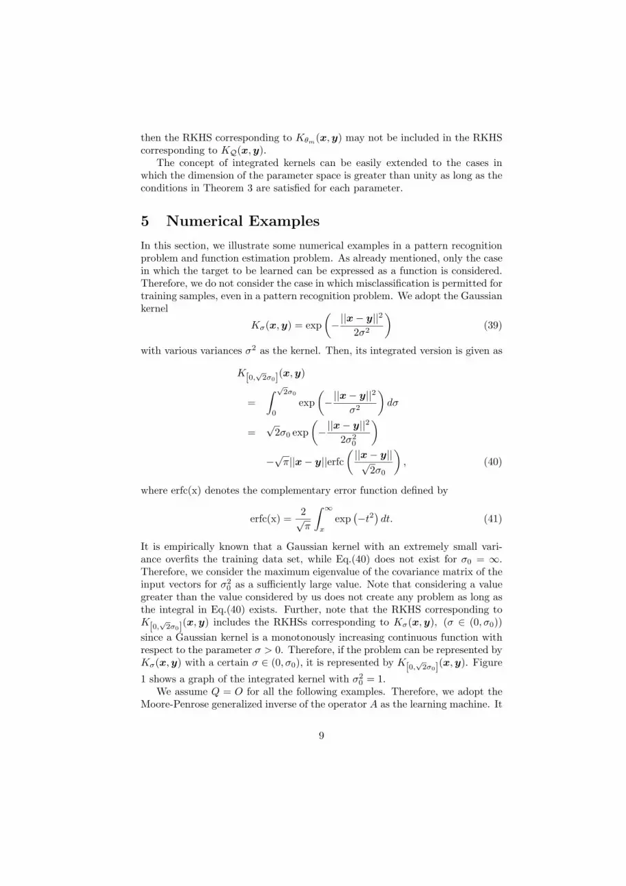
In this section, we illustrate some numerical examples in a pattern recognitionproblem and function estimation problem. As already mentioned, only the casein which the target to be learned can be expressed as a function is considered.Therefore, we do not consider the case in which misclassification is permitted fortraining samples, even in a pattern recognition problem. We adopt the Gaussiankernel

Kσ(x, y) = exp(−||x − y||2

2σ2

)(39)

with various variances σ2 as the kernel. Then, its integrated version is given as

K[0,√

2σ0](x, y)

=∫ √

2σ0

0

exp(−||x − y||2

σ2

)dσ

=√

2σ0 exp(−||x − y||2

2σ20

)−√

π||x − y||erfc(||x − y||√

2σ0

), (40)

where erfc(x) denotes the complementary error function defined by

erfc(x) =2√π

∫ ∞

x

exp(−t2

)dt. (41)

It is empirically known that a Gaussian kernel with an extremely small vari-ance overfits the training data set, while Eq.(40) does not exist for σ0 = ∞.Therefore, we consider the maximum eigenvalue of the covariance matrix of theinput vectors for σ2

0 as a sufficiently large value. Note that considering a valuegreater than the value considered by us does not create any problem as long asthe integral in Eq.(40) exists. Further, note that the RKHS corresponding toK[0,

√2σ0](x, y) includes the RKHSs corresponding to Kσ(x, y), (σ ∈ (0, σ0))

since a Gaussian kernel is a monotonously increasing continuous function withrespect to the parameter σ > 0. Therefore, if the problem can be represented byKσ(x, y) with a certain σ ∈ (0, σ0), it is represented by K[0,

√2σ0](x, y). Figure

1 shows a graph of the integrated kernel with σ20 = 1.

We assume Q = O for all the following examples. Therefore, we adopt theMoore-Penrose generalized inverse of the operator A as the learning machine. It

9

should be noted that the issue under consideration is not the learning machinebut the kernel itself.

5.1 Example of the Pattern Recognition Problem

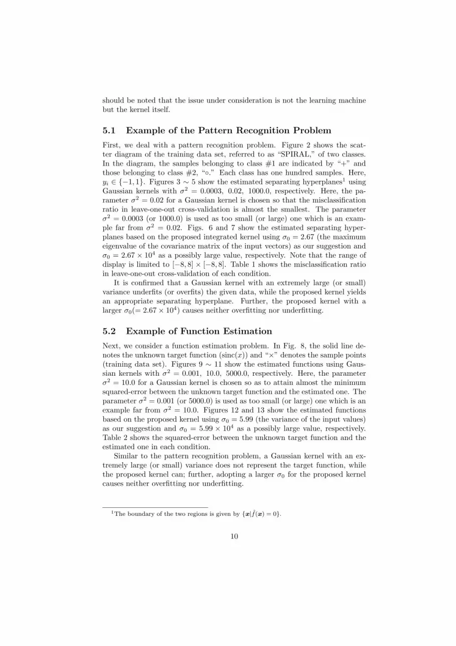
First, we deal with a pattern recognition problem. Figure 2 shows the scat-ter diagram of the training data set, referred to as “SPIRAL,” of two classes.In the diagram, the samples belonging to class #1 are indicated by “+” andthose belonging to class #2, “◦.” Each class has one hundred samples. Here,yi ∈ {−1, 1}. Figures 3 ∼ 5 show the estimated separating hyperplanes1 usingGaussian kernels with σ2 = 0.0003, 0.02, 1000.0, respectively. Here, the pa-rameter σ2 = 0.02 for a Gaussian kernel is chosen so that the misclassificationratio in leave-one-out cross-validation is almost the smallest. The parameterσ2 = 0.0003 (or 1000.0) is used as too small (or large) one which is an exam-ple far from σ2 = 0.02. Figs. 6 and 7 show the estimated separating hyper-planes based on the proposed integrated kernel using σ0 = 2.67 (the maximumeigenvalue of the covariance matrix of the input vectors) as our suggestion andσ0 = 2.67 × 104 as a possibly large value, respectively. Note that the range ofdisplay is limited to [−8, 8] × [−8, 8]. Table 1 shows the misclassification ratioin leave-one-out cross-validation of each condition.

It is confirmed that a Gaussian kernel with an extremely large (or small)variance underfits (or overfits) the given data, while the proposed kernel yieldsan appropriate separating hyperplane. Further, the proposed kernel with alarger σ0(= 2.67 × 104) causes neither overfitting nor underfitting.

5.2 Example of Function Estimation

Next, we consider a function estimation problem. In Fig. 8, the solid line de-notes the unknown target function (sinc(x)) and “×” denotes the sample points(training data set). Figures 9 ∼ 11 show the estimated functions using Gaus-sian kernels with σ2 = 0.001, 10.0, 5000.0, respectively. Here, the parameterσ2 = 10.0 for a Gaussian kernel is chosen so as to attain almost the minimumsquared-error between the unknown target function and the estimated one. Theparameter σ2 = 0.001 (or 5000.0) is used as too small (or large) one which is anexample far from σ2 = 10.0. Figures 12 and 13 show the estimated functionsbased on the proposed kernel using σ0 = 5.99 (the variance of the input values)as our suggestion and σ0 = 5.99 × 104 as a possibly large value, respectively.Table 2 shows the squared-error between the unknown target function and theestimated one in each condition.

Similar to the pattern recognition problem, a Gaussian kernel with an ex-tremely large (or small) variance does not represent the target function, whilethe proposed kernel can; further, adopting a larger σ0 for the proposed kernelcauses neither overfitting nor underfitting.

1The boundary of the two regions is given by {x|f̂(x) = 0}.

10

5.3 Remarks

It is often considered that complex models tend to overfit a training data set.However, this is not always true. The above numerical examples illustrate thecounterexamples. Indeed, the RKHS corresponding to the integrated kernel islarger than those corresponding to the integrand and the complexity of the largerRKHS is higher than that of the smaller RKHS on the basis of the Rademacheraverages (see [2] for instance).

In this paper, we assumed that what to be estimated is a function, whichmeans that our framework is only applicable to the classification problem inwhich the misclassification is not allowed for the given training data set. More-over, our discussion is only on the kernel (model) selection, and does not reachto the learning machine construction. Thus, in order to apply our kernel toreal-world problems, we have to resolve these problems theoretically.

6 Conclusion

In this study, on the basis of the framework of projection learning, we haveproposed a new method of constructing a kernel that incorporates the param-eter integration of parameterized kernels. The RKHS that corresponds to theproposed integrated kernel includes almost all the RKHSs that correspond tothe integrand with the parameters belonging to the intervals of integration. Thekernel used in this study does not require an optimization of parameter value,although a parameterized kernel often requires this optimization. The validityof the proposed kernel is confirmed by some artificial numerical examples.

Acknowledgments

This work was partially supported by Grant-in-Aid No.18700001 for Young Sci-entists (B) from the Ministry of Education, Culture, Sports and Technology ofJapan. The authors would like to thank Dr. Sugiyama and Dr. Takigawa fortheir valuable comments. The authors would also like to thank Dr. Kitamurafor his useful comments regarding the style of the revised manuscript.

References

[1] K. Muller, S. Mika, G. Ratsch, K. Tsuda, B. Scholkopf, An introduction tokernel-based learning algorithms, IEEE Transactions on Neural Networks12 (2001) 181–201.

[2] J. Shawe-Taylor, N. Cristianini, Kernel Methods for Pattern Recognition,Cambridge University Press, Cambridge, 2004.

11

[3] N. Cristianini, J. Shawe-Taylor, An Introduction to Support Vector Ma-chines and other kernel-based learning methods, Cambridge UniversityPress, Cambridge, 2000.

[4] N. Aronszajn, Theory of Reproducing Kernels, Transactions of the Ameri-can Mathematical Society 68 (3) (1950) 337–404.

[5] H. Ogawa, Neural Networks and Generalization Ability, IEICE TechnicalReport NC95-8 (1995) 57–64.

[6] M. Sugiyama, H. Ogawa, Incremental Projection Learning for OptimalGeneralization, Neural Networks 14 (1) (2001) 53–66.

[7] E. Oja, H. Ogawa, Parametric Projection Filter for Image and SignalRestoration, IEEE Transactions on Acoustics, Speech and Signal Process-ing ASSP–34 (6) (1986) 1643–1653.

[8] H. Imai, A. Tanaka, M. Miyakoshi, The family of parametric projectionfilters and its properties for perturbation, The IEICE Transactions on In-formation and Systems E80–D (8) (1997) 788–794.

[9] M. Sugiyama, H. Ogawa, Incremental construction of projection general-izing neural networks, IEICE Transactions on Information and SystemsE85-D (9) (2002) 1433–1442.

[10] V. N. Vapnik, The Nature of Statistical Learning Theory, Springer, NewYork, 1999.

[11] R. Schatten, Norm Ideals of Completely Continuous Operators, Springer-Verlag, Berlin, 1960.

[12] C. R. Rao, S. K. Mitra, Generalized Inverse of Matrices and its Applica-tions, John Wiley & Sons, 1971.

[13] M. Sugiyama, H. Ogawa, Subspace Information Criterion for Model Selec-tion, Neural Computation 13 (8) (2001) 1863–1889.

[14] S. Saitoh, Integral Transforms, Reproducing Kernels and Their Applica-tions, Addison Wesley Longman Ltd, UK, 1997.

12

Akira Tanakareceived his B.E. degree in 1994; M.E. degree, 1996; and D.E. degree, 2000

from Hokkaido University, Japan. He joined the Graduate School of InformationScience and Technology, Hokkaido University. His research interests includeimage processing, acoustic signal processing, and learning theory.

Hideyuki Imaireceived his D.E. degree in 1999 from Hokkaido University, Japan. He joined

the Graduate School of Information Science and Technology, Hokkaido Univer-sity. His research interests include statistical inferences.

Mineichi Kudoreceived his B.E. degree in 1983; M.E. degree, 1985; and D.E. degree, 1988

from Hokkaido University, Japan. He joined the Graduate School of Informa-tion Science and Technology, Hokkaido University. His current research in-terests include the design of pattern classifiers, machine learning, data analy-sis/representation, and image processing.

Masaaki Miyakoshireceived his D.E. degree in 1985 from Hokkaido University, Japan. He joined

the Graduate School of Information Science and Technology, Hokkaido Univer-sity. His research interests include fuzzy theory.

13

0

0.2

0.4

0.6

0.8

1

1.2

1.4

1.6

-4 -2 0 2 4

Figure 1: The graph of the integrated kernel K[0,√

2σ0] with σ20 = 1. The

horizontal axis denotes ||x − y||.

Figure 2: The scatter diagram of the training data set SPIRAL.

14

Figure 3: The result based on a Gaussian kernel with σ2 = 0.0003 for SPIRAL.

Figure 4: The result based on a Gaussian kernel with σ2 = 0.02 for SPIRAL.

15

Figure 5: The result based on a Gaussian kernel with σ2 = 1000 for SPIRAL.

Figure 6: The result based on the proposed integrated kernel for SPIRAL withσ0 = 2.67.

16

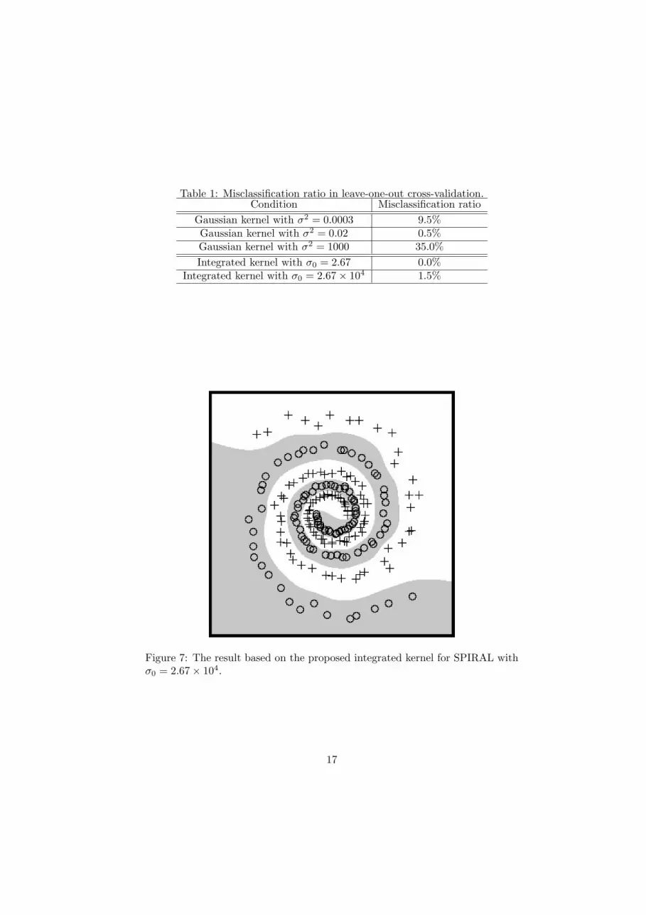
Table 1: Misclassification ratio in leave-one-out cross-validation.Condition Misclassification ratio

Gaussian kernel with σ2 = 0.0003 9.5%Gaussian kernel with σ2 = 0.02 0.5%Gaussian kernel with σ2 = 1000 35.0%Integrated kernel with σ0 = 2.67 0.0%

Integrated kernel with σ0 = 2.67 × 104 1.5%

Figure 7: The result based on the proposed integrated kernel for SPIRAL withσ0 = 2.67 × 104.

17

-0.4

-0.2

0

0.2

0.4

0.6

0.8

1

1.2

-10 -5 0 5 10

original

samples

Figure 8: Target function and training samples.

-0.4

-0.2

0

0.2

0.4

0.6

0.8

1

1.2

-10 -5 0 5 10

original

Gaussian(0.001)

Figure 9: The result based on a Gaussian kernel with σ2 = 0.001.

18

-0.4

-0.2

0

0.2

0.4

0.6

0.8

1

1.2

-10 -5 0 5 10

original

Gaussian(10.0)

Figure 10: The result based on a Gaussian kernel with σ2 = 10.0.

-0.4

-0.2

0

0.2

0.4

0.6

0.8

1

1.2

-10 -5 0 5 10

original

Gaussian(5000.0)

Figure 11: The result based on a Gaussian kernel with σ2 = 5000.0.

19

-0.4

-0.2

0

0.2

0.4

0.6

0.8

1

1.2

-10 -5 0 5 10

original

proposed

Figure 12: The result based on the proposed kernel with σ0 = 5.99.

-0.4

-0.2

0

0.2

0.4

0.6

0.8

1

1.2

-10 -5 0 5 10

original

proposed

Figure 13: The result based on the proposed kernel with σ0 = 5.99 × 104.

20

Table 2: The squared-error between the unknown true function and the esti-mated one.

Condition Squared-errorGaussian kernel with σ2 = 0.001 2.41Gaussian kernel with σ2 = 10.0 5.39 × 10−13

Gaussian kernel with σ2 = 5000 1.34Integrated kernel with σ0 = 5.99 2.74 × 10−4

Integrated kernel with σ0 = 5.99 × 104 2.70 × 10−4

21