Embed Size (px)
Citation preview

From Relations to XML: Cleaning, Integrating
and Securing Data
Xibei Jia
TH
E
U N I V E RS
IT
Y
OF
ED I N B U
RG
H
Doctor of Philosophy
Laboratory for Foundations of Computer Science
School of Informatics
University of Edinburgh
2007

AbstractWhile relational databases are still the preferred approach for storing data, XML is emerg-ing as the primary standard for representing and exchanging data. Consequently, it hasbeen increasingly important to provide a uniform XML interface to various data sources —integration; and critical to protect sensitive and confidential information in XML data —access control. Moreover, it is preferable to first detect and repair the inconsistencies inthe data to avoid the propagation of errors to other data processing steps. In response tothese challenges, this thesis presents an integrated framework for cleaning, integrating andsecuring data.
The framework contains three parts. First, the data cleaning sub-framework makesuse of a new class of constraints specially designed for improving data quality, referredto as conditional functional dependencies (CFDs), to detect and remove inconsistencies inrelational data. Both batch and incremental techniques are developed for detecting CFD
violations by SQL efficiently and repairing them based on a cost model. The cleaned rela-tional data, together with other non-XML data, is then converted to XML format by usingwidely deployed XML publishing facilities. Second, the data integration sub-frameworkuses a novel formalism, XML integration grammars (XIGs), to integrate multi-source XML
data which is either native or published from traditional databases. XIGs automaticallysupport conformance to a target DTD, and allow one to build a large, complex integrationvia composition of component XIGs. To efficiently materialize the integrated data, algo-rithms are developed for merging XML queries in XIGs and for scheduling them. Third, toprotect sensitive information in the integrated XML data, the data security sub-frameworkallows users to access the data only through authorized views. User queries posed on theseviews need to be rewritten into equivalent queries on the underlying document to avoid theprohibitive cost of materializing and maintaining large number of views. Two algorithmsare proposed to support virtual XML views: a rewriting algorithm that characterizes therewritten queries as a new form of automata and an evaluation algorithm to execute theautomata-represented queries. They allow the security sub-framework to answer querieson views in linear time.
Using both relational and XML technologies, this framework provides a uniform ap-proach to clean, integrate and secure data. The algorithms and techniques in the frameworkhave been implemented and the experimental study verifies their effectiveness and effi-ciency.
i

Acknowledgements
First and foremost, I would like to thank my supervisor Wenfei Fan. His insight has shaped
my research. He led me to the area of database systems, taught me how to do research,
encouraged me to aim high and provided me with invaluable help. Without him, this thesis
would not have been possible.
I am also indebted to my second supervisor Peter Buneman. His scholarship and advice
have broadened my scope of knowledge. He created a great database research environment
in Edinburgh and gave me plenty of chances to communicate with other researchers. I
benefited a lot from his guidance and support over the last few years.
I would like to thank my collaborators Philip Bohannon, Byron Choi, Gao Cong, Irini
Fundulaki, Minos Garofalakis, Floris Geerts, Anastasios Kementsietsidis, Shuai Ma and
Ming Xiong for their contributions to the various projects I have participated. In par-
ticularly, I am deeply gratitude to Floris Geerts and Anastasios Kementsietsidis for their
constant encouragement, generous help and stimulating discussions with me. I learned a
lot from working with them.
My special thanks go to Kousha Etessami and Michael Benedikt for serving as my
examiners.
I would also like to acknowledge all the members of the database group. I greatly
enjoyed the time spent with them.
Last but not least, I would like to thank my parents and my wife, for their love, support,
encouragement and care over the years.
ii

Declaration
I declare that this thesis was composed by myself, that the work contained herein is my
own except where explicitly stated otherwise in the text, and that this work has not been
submitted for any other degree or professional qualification except as specified.
(Xibei Jia)
iii

Table of Contents
1 Introduction 11.1 Real-world data is dirty, distributed and sensitive . . . . . . . . . . . . . . 1
1.1.1 Real world data needs to be cleaned . . . . . . . . . . . . . . . . . 3
1.1.2 The cleaned data needs to be integrated . . . . . . . . . . . . . . . 4
1.1.3 The integrated data needs to be protected . . . . . . . . . . . . . . 5
1.2 The CLINSE Framework for Cleaning, Integrating and Securing Data . . . 6
1.2.1 Clean data with Conditional Functional Dependencies . . . . . . . 7
1.2.2 Integrate data with XML Integration Grammars . . . . . . . . . . . 9
1.2.3 Secure data with XML security views . . . . . . . . . . . . . . . . 10
1.3 Outline of Dissertation . . . . . . . . . . . . . . . . . . . . . . . . . . . . 13
2 Cleaning Relational Data: Background and the State of the Art 142.1 Dirty data versus clean data: how to define it . . . . . . . . . . . . . . . . . 14
2.2 The dirty data to be cleaned: how to model it . . . . . . . . . . . . . . . . 16
2.3 Constraint-based data cleaning . . . . . . . . . . . . . . . . . . . . . . . . 19
2.3.1 Constraints. . . . . . . . . . . . . . . . . . . . . . . . . . . . . . . 20
2.3.2 Minimization measures. . . . . . . . . . . . . . . . . . . . . . . . 22
2.3.3 Query-oriented data cleaning: consistent query answering . . . . . 24
2.3.4 Repair-oriented data cleaning: constraint repair . . . . . . . . . . . 28
2.4 Edit-based data cleaning: statistical data editing and imputation . . . . . . . 30
2.5 Beyond rule-based data cleaning . . . . . . . . . . . . . . . . . . . . . . . 34
2.6 Summary . . . . . . . . . . . . . . . . . . . . . . . . . . . . . . . . . . . 35
iv

3 Modeling the Consistency of Data 373.1 Conditional Functional Dependencies . . . . . . . . . . . . . . . . . . . . 40
3.2 Detecting CFD Violations . . . . . . . . . . . . . . . . . . . . . . . . . . . 43
3.2.1 Checking a CFD with SQL . . . . . . . . . . . . . . . . . . . . . . 43
3.2.2 Incremental CFD Detection . . . . . . . . . . . . . . . . . . . . . 46
3.3 Experimental Study: Detecting CFD Violations . . . . . . . . . . . . . . . 52
3.3.1 Experimental Setup . . . . . . . . . . . . . . . . . . . . . . . . . . 53
3.3.2 Detecting CFD Violations . . . . . . . . . . . . . . . . . . . . . . . 54
3.3.3 Incremental CFD Detection . . . . . . . . . . . . . . . . . . . . . . 57
4 Repairing the Inconsistent Data 604.1 Data Cleaning Sub-framework . . . . . . . . . . . . . . . . . . . . . . . . 61
4.1.1 Violations and Repair Operations . . . . . . . . . . . . . . . . . . 61
4.1.2 Cost Model . . . . . . . . . . . . . . . . . . . . . . . . . . . . . . 62
4.1.3 An Overview of Data Cleaning Sub-framework . . . . . . . . . . . 65
4.2 An Algorithm for Finding Repairs . . . . . . . . . . . . . . . . . . . . . . 66
4.2.1 Resolving CFD Violations . . . . . . . . . . . . . . . . . . . . . . 68
4.2.2 Batch Repair Algorithm . . . . . . . . . . . . . . . . . . . . . . . 70
4.3 An Incremental Repairing Algorithm . . . . . . . . . . . . . . . . . . . . . 73
4.3.1 Incremental Algorithm and Local Repairing Problem . . . . . . . . 74
4.3.2 Ordering for Processing Tuples and Optimizations . . . . . . . . . 78
4.3.3 Applying INCREPAIR in the Non-incremental Setting . . . . . . . . 79
4.4 Experimental Study: Repairing CFD Violations . . . . . . . . . . . . . . . 80
4.4.1 Experimental Setting . . . . . . . . . . . . . . . . . . . . . . . . . 80
4.4.2 Experimental Results . . . . . . . . . . . . . . . . . . . . . . . . . 82
5 From Relation to XML 865.1 XML Data Model . . . . . . . . . . . . . . . . . . . . . . . . . . . . . . . 88
5.2 XML Data Definition . . . . . . . . . . . . . . . . . . . . . . . . . . . . . 91
5.3 XML Data Manipulation . . . . . . . . . . . . . . . . . . . . . . . . . . . 95
5.4 XML Views . . . . . . . . . . . . . . . . . . . . . . . . . . . . . . . . . . 99
5.5 XML Publishing . . . . . . . . . . . . . . . . . . . . . . . . . . . . . . . 101
v

5.6 Summary . . . . . . . . . . . . . . . . . . . . . . . . . . . . . . . . . . . 105
6 Schema Directed Integration of the Cleaned Data 1066.1 XML Integration Grammars (XIGs) . . . . . . . . . . . . . . . . . . . . . . 112
6.2 Case Study . . . . . . . . . . . . . . . . . . . . . . . . . . . . . . . . . . 117
6.3 XML Integration Sub-framework . . . . . . . . . . . . . . . . . . . . . . . 119
6.4 XIG Evaluation and Optimization . . . . . . . . . . . . . . . . . . . . . . 125
6.5 Experimental Evaluation . . . . . . . . . . . . . . . . . . . . . . . . . . . 132
6.6 Related Work . . . . . . . . . . . . . . . . . . . . . . . . . . . . . . . . . 135
7 Selective Exposure of the Integrated Data 1387.1 XML Security Sub-framework . . . . . . . . . . . . . . . . . . . . . . . . 141
7.2 XML Queries and View Specifications . . . . . . . . . . . . . . . . . . . . 143
7.2.1 XPath and Regular XPath . . . . . . . . . . . . . . . . . . . . . . 143
7.2.2 XML Views . . . . . . . . . . . . . . . . . . . . . . . . . . . . . . 144
7.3 The Closure Property of (Regular) XPath . . . . . . . . . . . . . . . . . . 147
7.4 Mixed Finite State Automata . . . . . . . . . . . . . . . . . . . . . . . . . 150
7.5 Rewriting Algorithm . . . . . . . . . . . . . . . . . . . . . . . . . . . . . 156
7.6 Evaluation Algorithm . . . . . . . . . . . . . . . . . . . . . . . . . . . . . 162
7.7 Optimizing Regular XPath Evaluation . . . . . . . . . . . . . . . . . . . . 167
7.7.1 The Type-Aware XML (TAX) index . . . . . . . . . . . . . . . . . 167
7.7.2 The Optimization Algorithm . . . . . . . . . . . . . . . . . . . . . 170
7.8 Experimental Study . . . . . . . . . . . . . . . . . . . . . . . . . . . . . . 173
7.9 Related Work . . . . . . . . . . . . . . . . . . . . . . . . . . . . . . . . . 175
8 Conclusions and Future Directions 179
Bibliography 183
vi

Chapter 1
Introduction
Since the 1970s, relational databases have been widely used in managing large volumes
of data. Whenever you call a friend, withdraw some money or book a flight, relational
databases are working behind the scene. With the wide adoption of relational databases,
more and more data has been accumulated and becomes one of the most valuable assets
of an organization. The value of the data heavily relies on its usability. Unfortunately, the
data in real-world organizations often has various problems which prevent it being used
directly.
1.1 Real-world data is dirty, distributed and sensitive
Traditional database technologies are designed for the settings in which data is stored in
well designed database management systems. However, in modern organizations, with the
ubiquity of electronic information, the data is distributed in far more diverse information
systems with various capabilities, including relational or object-oriented databases, XML
repositories, content management systems, etc. The following example demonstrates the
complexity of the data in a real world organization.
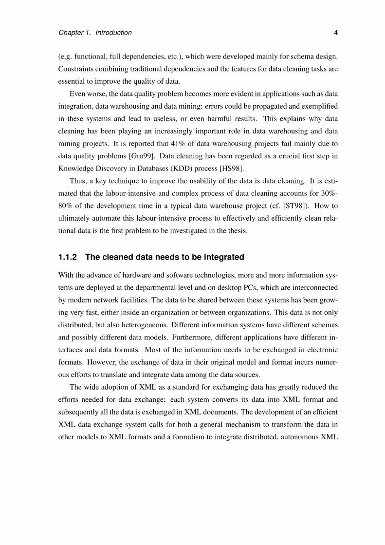
Example 1.1: Consider an automobile company which has accumulated a large volume
of data in its operations. As illustrated in Figure 1.1, this data includes the information
about its employees, customers, sales, products and services. Among them, the sales data
is kept in a centrally managed database, which is evolved from the legacy systems running
on the mainframe at the headquarter. The management of other data is far more complex.
1

Chapter 1. Introduction 2
SalesDB
Car FeatureDescriptions
Applications
DealerDB
DesignDB
Object
LDAPServer
DealerDB
MarketingDB
DesignDocuments
...
Figure 1.1: The data in an automobile company
The customer data is spread through the databases in the dealers, the sales department and
the service department. Prospective customer data, which is not as reliable as the data for
existing customers, is maintained in the marketing department. The car design data is in an
object-oriented database and the manufacture data is in a relational database. The design
documents are managed by a content management system in ODF or Docbook format (both
are standards for representing documents in XML). The car feature descriptions, which
need to be exchanged with dealers, are maintained in an XML repository. A part of the
employee data is in the LDAP server, while other parts are in a database in the human
resource department.
Suppose that an application assisting car sales needs to collect data about the customers,
employees, sales, car designs and features. A number of problems make it hard to develop
such kind of applications:
• the data is distributed into different locations: it is scattered across different depart-
ments and dealers.
• the data is heterogeneous: it is in different models such as relational models, object-
oriented models, XML data models and even the hierarchical LDAP data models.
• the data is autonomous: it is managed by independent information systems, defined
by different schemas.

Chapter 1. Introduction 3
• the data is sensitive: some data contains private information of employees or cus-
tomers; some data is confidential information for the company; some data is business
secrets between the company and its dealers.
• the data is in various qualities: some data, such as the employee data, is in high
quality; some data, such as the customer data, contains lots of errors due to inaccurate
data entry (the customer data in the marketing department) or the evolution of the
databases (the customer data in the dealers).
If this application is built directly, it has to be adapted to different data models and infor-
mation systems, various data qualities and diversified security mechanisms. Even worse,
there could be a large number of applications which rely on the data and for each one these
adaptation steps need to be repeated. It is vastly desirable to prepare the data in a general,
uniform framework before feeding them into such applications. 2
The complex nature of the real-word data means that no single technology can resolve
all the problems associated with them. Different technologies need to be utilized to improve
different aspects of the data. These aspects are classified into three categories and the
techniques used to improve them are discussed below.
1.1.1 Real world data needs to be cleaned
Dirty data is everywhere. Do you have experience of receiving letters addressed to people
who moved out long ago? Such a mistake is caused by dirty data. A recent survey [Red98]
reveals that enterprises typically expect data error rates of approximately 1%–5%. The
consequences caused by dirty data may be severe. It has been estimated that poor quality
customer data costs U.S. businesses $611 billion annually in postage, printing and staff
overhead (cf. [Eck02]). The process of detecting and removing errors and inconsistencies
from the data in order to improve its quality is referred to as data cleaning [RD00].
The data quality problem may arise in any information system, particularly in those
systems where the integrity constraints can not be or have not been enforced. In fact, even
in databases with well defined integrity constraints, errors are still common. In a widely
used, comprehensive taxonomy of dirty data [KCH+03], wrong data which can not be pre-
vented by traditional integrity constraints present a large category of dirty data. However,
most existing constraint-based data cleaning research is based on traditional dependencies
Chapter 1. Introduction 4
(e.g. functional, full dependencies, etc.), which were developed mainly for schema design.
Constraints combining traditional dependencies and the features for data cleaning tasks are
essential to improve the quality of data.
Even worse, the data quality problem becomes more evident in applications such as data
integration, data warehousing and data mining: errors could be propagated and exemplified
in these systems and lead to useless, or even harmful results. This explains why data
cleaning has been playing an increasingly important role in data warehousing and data
mining projects. It is reported that 41% of data warehousing projects fail mainly due to
data quality problems [Gro99]. Data cleaning has been regarded as a crucial first step in
Knowledge Discovery in Databases (KDD) process [HS98].
Thus, a key technique to improve the usability of the data is data cleaning. It is esti-
mated that the labour-intensive and complex process of data cleaning accounts for 30%-
80% of the development time in a typical data warehouse project (cf. [ST98]). How to
ultimately automate this labour-intensive process to effectively and efficiently clean rela-
tional data is the first problem to be investigated in the thesis.
1.1.2 The cleaned data needs to be integrated
With the advance of hardware and software technologies, more and more information sys-
tems are deployed at the departmental level and on desktop PCs, which are interconnected
by modern network facilities. The data to be shared between these systems has been grow-
ing very fast, either inside an organization or between organizations. This data is not only
distributed, but also heterogeneous. Different information systems have different schemas
and possibly different data models. Furthermore, different applications have different in-
terfaces and data formats. Most of the information needs to be exchanged in electronic
formats. However, the exchange of data in their original model and format incurs numer-
ous efforts to translate and integrate data among the data sources.
The wide adoption of XML as a standard for exchanging data has greatly reduced the
efforts needed for data exchange: each system converts its data into XML format and
subsequently all the data is exchanged in XML documents. The development of an efficient
XML data exchange system calls for both a general mechanism to transform the data in
other models to XML formats and a formalism to integrate distributed, autonomous XML

Chapter 1. Introduction 5
data into a single XML document.
The former, often referred to as XML publishing, has been investigated for several years.
A number of prototype systems for XML publishing, for instance, SilkRoute [FTS00],
XPERANTO [CKS+00] and PRATA+ [CFJK04] have been built with great success. More-
over, most mainstream database management systems have provided XML publishing
functionalities.
The latter, referred to as XML integration, however, has not attracted as much research
as XML publishing. In contrast with data integration in the relational context, new require-
ments have been imposed to XML data integration. First, both the source data and the
integrated data are in XML model. Second, an integrated view always needs to be ma-
terialized in order to be sent to other parties. Third and most importantly, the integrated
XML document is usually required to conform to an existing public schema defined by a
standard, a community or an application. Last, building a system to efficiently integrate
distributed data into a complex XML document requires not only a flexible framework but
also sophisticated optimization techniques. Although several XML data integration sys-
tems exist, none of them addresses all of the above issues. XML data integration is the
focus of the second part of the thesis.
1.1.3 The integrated data needs to be protected
The data exchanged between applications often contains sensitive information such as busi-
ness secrets. Any unintended disclosure of the information would cause severe problems.
The success of any information system does not only depend on the quality and the inte-
gration of the data, but also relies on the effective protection of this valuable, yet sensitive
data. The security problem appears throughout the life cycle of the data, from its genera-
tion, storage, manipulation, to its integration, exchange and disposal. Lots of techniques
exist for securing data in some of these processes. For example, most of the source data
could be protected by the security mechanisms built into the source systems, such as DBMS
or OS; the transmission of the data through network could be protected by secure network
protocols... However, no matured technologies exist to secure the integrated XML data.
The protection of the integrated data calls for a generic, flexible security model that can
effectively control access to XML data at various levels of granularity. The access control

Chapter 1. Introduction 6
in relational databases is driven by views: security administrators specify views for each
user group; subsequently, any user is allowed to access the data only through a view over
it. It is natural to extend this view mechanism into XML data management.
Even more importantly, enforcing such access control models should not imply any
drastic degradation in either performance or functionality for the underlying XML query
engine. In this sense these views need to be kept virtual because the number of views to be
materialized could be prohibitively large due to the large number of user groups. Although
relational views are widely available in all mainstream database systems, no virtual XML
views are supported by any XML data management system, particularly when the views
are recursively defined. In the last part of the thesis, the query rewriting and evaluation
techniques are developed to support the enforcement of XML access control through virtual
views. Given the ubiquitous of XML in modern information systems, this virtue view
mechanism is not only critical to access control, but also increasingly demanded in other
XML related contexts.
1.2 The CLINSE Framework for Cleaning, Integrating and
Securing Data
In order to make effective and efficient use of the dirty, distributed and sensitive data, novel
formalisms, algorithms and techniques are called for to clean, integrate and secure this
data. This thesis addresses the challenges classified above in an integral framework, called
CLINSE (CLeaning, INtegrating and SEcuring data), which makes use of both relational
and XML data management techniques.
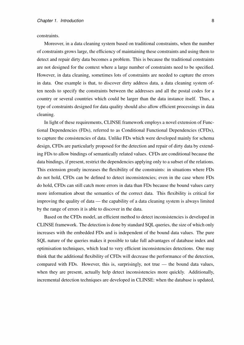
As shown in Figure 1.2, CLINSE framework has three parts. The relational data is first
processed by the data cleaning sub-framework to improve its quality. Then, the cleaned
relational data and the data in other non-XML sources are published into XML format.
Subsequently, the XML integration sub-framework extracts data from all the sources and
constructs a single XML document. At last, the XML security sub-framework ensures
that users can access the integrated XML data only through an authorized view in order
to protect the sensitive information. The models, methods and algorithms in these sub-
frameworks are introduced below.

Chapter 1. Introduction 7
IntegratedXML Data
XML DB
XMLDocuments
PublishedXML Data
PublishedXML Data
Virtual XML View
XML Integration
XM
L Secu
rity
Sub
-fra
mew
ork
XM
L In
tegra
tion
Sub-f
ram
ew
ork
RDB RDB
Data CleaningOO DB
Object
Data Cleaning Sub-framework
XML Publishing
Figure 1.2: CLINSE framework to clean, integrate and secure data
1.2.1 Clean data with Conditional Functional Dependencies
Dirty data in a database often emerges as violations of integrity constraints. As a result,
constraint-based technique is an important approach to clean data. In a constraint-based
data cleaning approach, the core is a set of constraints which are defined to model the
correctness of the data. Subsequently, potential errors are characterized as the inconsisten-
cies in the data with respect to those constraints. The quality of the data is improved by
detecting these inconsistencies and repairing them to restore the database to a consistent
state.
Few work [BFFR05, LB07b] on constraint-based data cleaning has been reported and
all of them use traditional database integrity constraints, such as functional dependencies,
inclusion dependencies or denial dependencies, to model the quality of data. Whereas, in
practice, these constraints are often not sufficient to improve the data quality. One reason
is that traditional integrity constraints are always supposed to hold on the whole database.
In a data cleaning context, due to schema evolution or data integration, it is common that
the constraints only hold for a subset of the data. This motivate us to bring conditions into
Chapter 1. Introduction 8
constraints.
Moreover, in a data cleaning system based on traditional constraints, when the number
of constraints grows large, the efficiency of maintaining these constraints and using them to
detect and repair dirty data becomes a problem. This is because the traditional constraints
are not designed for the context where a large number of constraints need to be specified.
However, in data cleaning, sometimes lots of constraints are needed to capture the errors
in data. One example is that, to discover dirty address data, a data cleaning system of-
ten needs to specify the constraints between the addresses and all the postal codes for a
country or several countries which could be larger than the data instance itself. Thus, a
type of constraints designed for data quality should also allow efficient processings in data
cleaning.
In light of these requirements, CLINSE framework employs a novel extension of Func-
tional Dependencies (FDs), referred to as Conditional Functional Dependencies (CFDs),
to capture the consistencies of data. Unlike FDs which were developed mainly for schema
design, CFDs are particularly proposed for the detection and repair of dirty data by extend-
ing FDs to allow bindings of semantically related values. CFDs are conditional because the
data bindings, if present, restrict the dependencies applying only to a subset of the relations.
This extension greatly increases the flexibility of the constraints: in situations where FDs
do not hold, CFDs can be defined to detect inconsistencies; even in the case where FDs
do hold, CFDs can still catch more errors in data than FDs because the bound values carry
more information about the semantics of the correct data. This flexibility is critical for
improving the quality of data — the capability of a data cleaning system is always limited
by the range of errors it is able to discover in the data.
Based on the CFDs model, an efficient method to detect inconsistencies is developed in
CLINSE framework. The detection is done by standard SQL queries, the size of which only
increases with the embedded FDs and is independent of the bound data values. The pure
SQL nature of the queries makes it possible to take full advantages of database index and
optimisation techniques, which lead to very efficient inconsistencies detections. One may
think that the additional flexibility of CFDs will decrease the performance of the detection,
compared with FDs. However, this is, surprisingly, not true — the bound data values,
when they are present, actually help detect inconsistencies more quickly. Additionally,
incremental detection techniques are developed in CLINSE: when the database is updated,

Chapter 1. Introduction 9
minimum work is needed to re-detect the inconsistencies.
Better still, the additional information of the correct data carried by the data bindings
provides more semantic information for repairing an inconsistent database. In fact, the
data binding could be seen as a general way to model domain knowledge in a data cleaning
framework. One advantage of modelling domain knowledge this way is its scalability: it is
treated as ordinary data tables in the database and its size is only limited by the capability
of the database system. CFDs provide a solid foundation for the automated repair and
incremental repair modules of the CLINSE framework.
As shown in [BFFR05], the problem of finding a quality repair is NP-complete even
for a fixed set of traditional FDs. This problem remains intractable for CFDs, and that
FD-based repairing algorithms may not even terminate when applied to CFDs. To this
end the cost model of [BFFR05] that incorporates both the accuracy of the data and edit
distance is adopted in CLINSE. Based on the cost model, The FD-based repairing heuristic
introduced in [BFFR05] is extended such that it is guaranteed to terminate and find quality
repairs when working on CFDs.
The problem for incrementally finding quality repairs does not make our lives easier: it
is also NP-complete. In light of this an efficient heuristic algorithm is developed for finding
repairs in response to updates, namely, deletions or insertions of a group of tuples. This
algorithm can also be used to find repairs of a dirty database.
The accuracy and scalability of these methods are evaluated with real data scraped from
the Web. The experiments shows that CFDs are able to catch inconsistencies that traditional
FDs fail to detect, and that the repairing and incremental repairing algorithms efficiently
find accurate candidate repairs for large datasets.
CFDs and the proposed algorithms are a promising tool for cleaning real-world data.
The algorithms developed in CLINSE are the first automated methods for finding repairs
and incrementally finding repairs based on conditional constraints.
1.2.2 Integrate data with XML Integration Grammars
An important new requirement for extending data integration from relational context to
XML context is the schema conformance. In relational databases, the schema is private to
the data management systems. Whereas, in XML data management, the schema is often
Chapter 1. Introduction 10
public and a large number of XML schemas are even standards. Consequently, the global
schema in XML data integration should be an input to the data integration system, rather
than being defined in the data integration process. No existing system which integrates data
from XML sources takes into account this requirement.
In CLINSE framework, a novel formalism, XML Integration Grammars (XIGs), is pro-
posed for specifying DTD-directed integration of XML data. Abstractly, an XIG maps
data from multiple XML sources to a target XML document that conforms to a predefined
DTD. An XIG extracts source XML data via queries expressed in a fragment of XQuery,
and controls target document generation with tree-valued attributes and the target DTD.
The novelty of XIGs consists in not only their automatic support for DTD-conformance
but also in their composability: an XIG may embed local and remote XIGs in its definition,
and invoke these XIGs during its evaluation. This yields an important modularity property
for the XIGs that allows one to divide a complex integration task into manageable sub-tasks
and conquer each of them separately.
Based on the XIG formalism, a sub-framework for DTD-directed XML integration,
including algorithms for efficiently evaluating XIGs, is developed in CLINSE. How to cap-
ture recursive DTDs and recursive XIGs in a uniform framework is demonstrated, and a
cost-based algorithm for scheduling local XIGs/XML queries and remote XIGs to maxi-
mize parallelism is proposed. An algorithm for merging multiple XQuery expressions into
a single query without using “outer-union/outer-join” is provided. Combined with possible
optimization techniques for the XQuery fragment used in XIG definitions, such optimiza-
tions can yield efficient evaluation strategies for DTD-directed XML integration.
1.2.3 Secure data with XML security views
To protect the sensitive integrated XML data, CLINSE adopts a view based security model
proposed in [FCG04]: (1) the security administrator specifies an access policy for each user
group by annotating the DTDs of an XML document; (2) a derivation module automatically
derives the definition of a security view for each user group which consists of all and
only the accessible information with respect to the policy specified for that group; (3)
meanwhile, a view schema characterizing the accessible data of the group is also derived
and provided to authorized users so that they can formulate their queries over the view.

Chapter 1. Introduction 11
This view based security model provides both schema availability, namely, view DTDs to
facilitate authorized users to formulate their queries, and access control, i.e., protection of
sensitive information from improper disclosure.
A central problem in a view based security framework is how to answer queries posed
on the views. One way to do this is first materializing the views and then directly evaluating
queries on the views. However, in XML security context, there are often a large number of
users for the same XML document, which lead to lots of user groups and views for those
groups. It is prohibitively expensive to materialize and maintain so many views. A realistic
approach is to rewrite (aka. translate, reformulate) queries on the views into equivalent
queries on the source, evaluate the rewritten queries on the source without materializing
the views, and return the answers to the users. This is the approach used in CLINSE.
Although there has been a host of work on answering queries posed on XML views over
relational data, little work has been done on querying virtual XML views over XML data,
where query rewriting has only been studied for non-recursive XML views, over which
XPath rewriting is always possible [FCG04]. Query rewriting for recursive views over
XML is still an open problem [KCKN04].
In CLINSE framework, the problem of answering queries posed on possibly recursive
views of XML documents is studied and efficient solutions are provided. It is shown that
XPath is not closed under query rewriting for recursive views. In light of this CLINSE uses
a mild extension of XPath, regular XPath [Mar04b], which uses the general Kleene closure
E∗ instead of the ‘//’ axis. This regular XPath is closed under rewriting for arbitrary views,
recursive or not. Since regular XPath subsumes XPath, any XPath queries on views can be
rewritten to equivalent regular XPath queries on the source.
However, the rewriting problem is EXPTIME-complete: for a (regular) XPath query Q
over even a non-recursive view, the rewritten regular XPath query on the source may be
inherently exponential in the size of Q and the view DTD DV . This tells us that rewriting is
beyond reach in practice if Q is directly rewritten into regular XPath.
To avoid this prohibitive cost, CLINSE uses a new form of automata, mixed finite state
automata (MFA) to represent rewritten regular XPath queries. An MFA is a nondeter-
ministic finite automaton (NFA) “annotated” with alternating finite state automata (AFA),
which characterize data-selection paths and filters of a regular XPath query Q, respec-
tively. The algorithm rewrites Q into an equivalent MFA M . In contrast to the exponential

Chapter 1. Introduction 12
blowup, the size of M is bounded by O(|Q||σ||DV |). This makes it possible to efficiently
answer queries on views via rewriting. To our knowledge, although a number of automaton
formalisms were proposed for XPath and XML stream (e.g. [DFFT02, GGM+04]), they
cannot characterize regular XPath queries, as opposed to MFA.
In CLINSE, an efficient algorithm, called HyPE, is provided for evaluating MFA M(rewritten regular XPath queries) on XML source T . While there have been a number
of evaluation algorithms developed for XPath, none is capable of processing automaton
represented regular XPath queries. Previous algorithms for XPath (e.g., [Koc03]) require
at least two passes of T : a bottom-up traversal of T to evaluate filters, followed by a top-
down pass of T to select nodes in the query answer. In contrast, HyPE combines the two
passes into a single top-down pass of T during which it both evaluates filters and identifies
potential answer nodes. The key idea is to use an auxiliary graph, often far smaller than
T , to store potential answer nodes. Then, a single traversal of the graph suffices to find the
actual answer nodes. The algorithm effectively avoids unnecessary processing of subtrees
of T that do not contribute to the query answer. It is not only an efficient algorithm for
evaluating regular XPath queries (MFA), but also an alternative algorithm to evaluate XPath
queries.
A novel indexing technique to optimize the evaluation of regular XPath queries is also
developed in CLINSE. While several labeling and indexing techniques were developed for
evaluating ‘//’ in XPath (e.g., [LM01, KMS02, SHYY05]), they are not very helpful when
computing the general Kleene closure E∗, where E is itself a regular XPath query which
may also contain a sub-query E∗1 . In contrast to previous labeling techniques, the indexing
structure in CLINSE summarizes, at each node, information about its descendants of all
different types in the document DTD. The indexing structure is effective in preventing
unnecessary traversal of subtrees during FA (regular XPath) evaluation. This technique is
in fact applicable to processing of XML queries beyond regular XPath.
The security sub-framework fully supports the rewriting and evaluation techniques men-
tioned above. An experimental study conducted on the system clearly demonstrates that the
HyPE evaluation techniques are efficient and scale well. For regular XPath queries, HyPE
evaluation of queries is compared with that of their XQuery translation, and it is found that
the latter requires considerably more time. Furthermore, HyPE outperforms the widely used
XPath engine Xalan (default XPath implementation in Java 5), whether Xalan uses its in-

Chapter 1. Introduction 13
terpretive processor or its high performance compiling processor (XSLTC), when evaluating
XPath queries.
In summary, the security sub-framework of CLINSE does not only provide effective
and efficient access control layer for the integrated XML data, but also contain the first
practical and complete solution for answering regular XPath queries posed on (virtual and
possibly recursively defined) XML views. It is provably efficient: it has a linear-time data
complexity and a quadratic combined complexity. Furthermore it yields the first efficient
technique for processing regular XPath queries, whose need is evident since regular XPath
is increasingly being used both as a stand-alone query language and as an intermediate
language in query translation [FYL+05].
1.3 Outline of Dissertation
The remainder of this thesis is organized as follows.
Chapter 2 provides background about cleaning relational data. It introduces the basic
methods of data cleaning and cites relevant work in these areas.
Chapter 3 formally defines CFDs, presents the SQL techniques for detecting and incre-
mentally detecting CFD violations, followed by the experimental study. This work is taken
from [BFG+07].
In Chapter 4, the algorithms for finding repairs and incrementally finding repairs are
developed and experimental results are presented. This work is taken from [CFG+07].
Chapter 5 explains how to publish the repaired relational data to XML format and pro-
vides background about XML data management.
Chapter 6 defines XIGs, followed by XIG examples, presents an XIG-based framework
for XML integration. It provides algorithms for evaluating XIGs, followed by experimental
results. This work is taken from [FGXJ04].
Chapter 7 discusses the closure property of (regular) XPath rewriting. Then, it intro-
duces MFA and describes the rewriting algorithm. It also presents the MFA evaluation
and optimization algorithms, followed by experimental results. This work is taken from
[FGJK07] and [FGJK06].
Chapter 8 concludes the thesis.

Chapter 2
Cleaning Relational Data: Background
and the State of the Art
Although a few special data cleaning problems, for example, data merge/purge (a.k.a.,
record linkage), have been studied for a long time, data cleaning in general is relatively
new compared with other established areas such as data integration and data mining which
have been widely investigated for more than a decade. The theories, models, algorithms
and systems for data cleaning are still in their early stages. However, the importance of
data cleaning has been increasingly recognized as more and more data warehousing and
data mining systems fail due to poor quality of data.
There are a lot of problems associated with data cleaning. What is dirty data? How
to model and discover errors in data? Which kind of dirty data could be repaired and
how to repair it? How to incorporate domain knowledge to assist data cleaning? How to
build a data cleaning system? Will the results of a fully automatic data cleaning method
be satisfiable? How to combine and trade-off human interactions in a semi-automatic data
cleaning framework? Some of these problems have been addressed in prior work.
2.1 Dirty data versus clean data: how to define it
The errors in data arise with various reasons:
• The data in an organization is often accumulated within a long period of time mea-
sured by years or even decades. The schemas and constraints changed time by time
14

Chapter 2. Cleaning Relational Data: Background and the State of the Art 15
in their history.
• No integrity constraints are defined on the data or the integrity is enforced in the
applications which are bypassed when the database is directly accessed.
• There are errors in data entry which can not be detected by integrity constraints.
• The data is mis-translated when it is integrated from different sources. . .
In [KCH+03], a comprehensive classification of dirty data is developed. In that taxon-
omy, the dirty data is classified hierarchically, with missing data, wrong data and unusable
data at the top level. The wrong data are further divided into wrong data due to non-
enforcement of enforceable constraints and that due to non-enforceability of constraints.
Although this taxonomy is very helpful for understanding the sources and forms of dirty
data, by no means it can serve as a definition of dirty data.
Interestingly, although a host of work has studied the concepts in data quality, there is
no widely accepted formal definition of clean data and dirty data. Early literature [Kri79,
BP85] uses correctness to define data quality. For instance, [BP85] regards the data in
which the recorded value is in conformity with the actual value as clean. However, the
clean data in one user’s eyes could be dirty in others’ eyes. Indeed, the correctness of
data, depends on its context and purpose. For example, an address value with only a mail
box could be regarded as correct in one application where postal address is required, while
incorrect in another application where home address is desired. It is hard, if possible, to
give a sound and complete formal definition for “error” or “dirty data” that is independent
of its context — all existing definitions are descriptive and contain only some types of
errors. Most recent work [Orr98, Wan98] adopts the concept of “fitness for use”: clean
data is defined as data that is fit for use by data consumers [WS96, SLW97]. This results
in a context dependent, multidimensional concept of clean and dirty data.
A lot of dimensions are used in data quality literature to define the dirtiness of data.
For example, [WS96] presents a survey of 179 dimensions suggested by various data
consumers. Accuracy, consistency, relevancy, completeness and timeliness are the most
frequently found dimensions in literature. A piece of data is accurate if it correctly repre-
sents the real world value. It is consistent if there are no conflicts in it. It is relevant if the
data and its granularity are of interest. It is complete if all needed information is included
and it is timely if it is up to date. Although each of the dimensions captures one aspect

Chapter 2. Cleaning Relational Data: Background and the State of the Art 16
of potential dirty data, these multidimensional definitions can not be used directly in data
cleaning.
2.2 The dirty data to be cleaned: how to model it
Since the definition of the dirty data is multi-dimensional, it would be natural to ask: which
dimensions are considered in data cleaning? In other words, what type of errors could be
cleaned?
At first glance, it seems that any dirty data can be detected and repaired, at worst, by
manually inspecting each value in the database by a domain expert. This is, however,
not true even if such a labour intensive process is affordable — some data is simply not
verifiable if no related information exists in the source or anywhere else. For example,
a transaction record of a customer’s shopping long time ago can not be verified if the
customer can not remember it and the log for this transaction in the store has been deleted.
Errors in data could be discovered and corrected only if there is sufficient information for
that piece of data from the same database, external sources, or both. For manual data
cleaning, these external sources could be the ones who input the data, or domain experts
in the application area. In automatic data cleaning, these external sources would be the
domain knowledge built into the data cleaning model.
Manual data cleaning is usually not affordable: it is laborious and time consuming.
Moreover, it is subjective and sometimes leads to bad repair. A widespread misunderstand-
ing is that manual repair always achieves better quality than automatic one. In practice, it
is not uncommon to get bad manual repair because of the insufficient information a domain
expert is aware of or make use of. In many cases it is not feasible for a domain expert
to retrieve and inspect all the relevant information required to produce a good repair, even
with the aids of some tools. Worse still, the expert will not know whether their repair will
be consistent or not with other data in the database until the repair is applied.
In (semi-)automatic data cleaning, instead of using the multidimensional concept of
dirty data, errors are defined within the scope of a model capturing the quality of data.
Therefore, in order to find out what type of errors could be cleaned, another related question
has to be answered: how do we model the data for the purpose of cleaning it?
The most widely used models for data cleaning are rule-based models. The idea of

Chapter 2. Cleaning Relational Data: Background and the State of the Art 17
using rules to improve data quality has long been practiced in data processing systems.
In many web applications, the user inputs are verified against a set of validation rules
encoded in scripting languages such as Java script to reduce the errors in data entry. In
database systems, integrity constraints, such as keys, foreign keys, are employed to prevent
undesired data from damaging the state of a database.
Different types of rules have been used for data cleaning. These rules are used to
characterize either clean or dirty data:
Constraints In relational databases, integrity constraints are used to ensure that no change
would be allowed if it destroys the consistency of data by enforcing predicates on
relations. These predicates have to be satisfied to correctly reflect the real world. In
general, an integrity constraint can be an arbitrary sentence from first-order logic per-
taining to the database. However, arbitrary predicates may be costly to test [SKS01c].
Functional dependencies and inclusion dependencies are examples of common in-
tegrity constraints found in database practice. In constraint-based data cleaning, a
set of constraints is defined to capture the semantics of clean data; subsequently, a
piece of data is inconsistent (containing errors) if it violates the constraints defined
in the model. These detected errors are then repaired to make the data consistent. In
other words, the errors detected and repaired in constraint-based models are incon-
sistencies in the data with respect to the constraints.
Association Rules [HGG01] proposes error detection techniques based on association
rules. Given sets of items X , Y in a collection of transactions, an association rule
is of the form X → Y which indicates that whenever a transaction contains all items
in X then it is likely to also contains all items in Y with a probability called rule
confidence. The basic idea for association-rule-based data cleaning is first generat-
ing association rules from the training data and then applying them to the evaluating
data. Usually the training data and evaluating data are originated from the same
data set. For each record in the data, some of these rules may be supported, some
rules may not be applicable to it, one or more rules may contradict with it. Finally a
score is computed for every record as the number of violated rules weighted by their
confidences. The records with high scores are suggested as potential errors. The
hypothesis behind this model is that the generated association rules capture the nor-

Chapter 2. Cleaning Relational Data: Background and the State of the Art 18
mality of the considered data. This is consistent with constraints: both of them are
used to characterize the regularities of clean data. The difference is that association
rules are mined from the data and the violations might not be errors sometimes. By
contrast, although nothing prevents constraints to be discovered from data, they are
usually composed by domain experts and a violation always suggest an error in the
conflicting data.
Edit Rules In data editing, an edit is a restriction to a single field in a record to ascertain
whether its value is valid, or to a combination of fields in a record to ascertain whether
the fields are consistent with one another. Here a record is a set of recorded answers to
all the questions on the questionnaire [FH76]. For example, in a single-field edit we
might want the number of children to be less than 20; in a multi-field edit we might
want an individual of less than 15 years to always have marital status of unmarried.
Data editing is the activity to detect and correct errors (logical inconsistencies) in
data, especially in survey data.
Cleansing Rules In practice, data cleaning is often conducted by a set of cleansing rules.
Each cleansing rule consists of two parts: a condition and an action which is trig-
gered when the condition is satisfied. The action could be simply reporting the error
detected, removing that record or repairing the involved values[Rit06]. An example
of cleansing rule is that whenever the value 1 occurs in the Gender field whose do-
main is M and F (condition), the value needs to be changed to F (action). Cleansing
rules are different from the above types of rules due to the fact that each rule has an
explicit action defined in it while none of the above types of rules have. This is a
procedural way to clean data, as contrast to the declarative means of the above three
types of rules. Cleansing rules are analogous to triggers in database systems. How-
ever, triggers are activated by the change of the state of a database; cleansing rules
are executed by users of a data cleaning system.
Of course, the above classification by no means reflects the theoretical properties of
the rules used in data cleaning and there are lots of overlaps between these categories. For
example, edits could be expressed as constraints in a form of logic and constraints can
be used as the conditions in cleansing rules. The purpose of this classification is to show

Chapter 2. Cleaning Relational Data: Background and the State of the Art 19
different views on data cleaning from different communities: database (constraints), data
mining (association rules), statistical research (edits) and industry (cleansing rules). In
particular, a lot of work has been done in the areas of constraint-based data cleaning and
statistical data editing. In the next two sections, we will review the research in those two
areas.
Most previous research on data cleaning falls into the above rule-based models. There
are a few exceptions, including the work using probabilistic models, clusters or patterns to
model the regularities in data. In these models, no explicit rules are discovered from data
or composed by domain experts. These models are discussed in Section 2.5.
This model based definition has a direct effect: an error in one model could be clean
data in the other model. From this point of view, no data cleaning framework is complete —
each framework can only find and fix the type of errors it models. The relative definition
also makes it difficult to compare different data cleaning methods due to the lack of a
consensus on the dirtiness of a value.
2.3 Constraint-based data cleaning
From the data cleaning point of view, there are three levels of dirty data:
1. the data in a database that is dirty according to the multidimensional concept of
fitness for use;
2. the dirty data that could be captured by the current model; and
3. the dirty data that could be captured by the model without additional information
beyond the database itself.
The first type of dirty data includes the second type and, in addition, it contains the dirty
data that can not be captured by the current model. Similarly, the second type of dirty
data includes the third type and it also contains the dirty data that could be captured with
additional domain knowledge. The range of dirty data a constraint-based system can deal
with is limited by its ability to enlarge the last two types of dirty data. Although lots of
dimensions are included in the first type of dirty data, only the consistency dimension is

Chapter 2. Cleaning Relational Data: Background and the State of the Art 20
captured by constraint-based models. Thus, one principle of constraint based data cleaning
is to maximize the dirty data characterized by the consistency dimension.
As long as dirty data in a database is captured as inconsistencies with respect to a set of
integrity constraints, a clean database, called a repair, could be computed to resolve these
inconsistencies. The concept of database repair is introduced in [ABC99], where a repair
is used as an auxiliary notion for defining consistent query answering, which will be dis-
cussed in Section 2.3.3. Obviously, in constraint-based data cleaning, a repair must satisfy
all constraints defined in the model, but there could be lots of such repairs for the same
database. For example, a repair can be obtained by simply remove all of the inconsistent
tuples repeatedly until a consistent database is obtained (this process needs to be repeated
when inclusion dependencies are presented). Therefore, the system should distinguish good
repairs from bad ones by certain computable measures. Following this principle, a database
repair is defined as follows:
A constraint-based data cleaning model consists a relational database D to be cleaned
and a set C of constraints defined on D to characterize the semantics of the data. Database
D is dirty if it is inconsistent under constraints C, i.e. D 6|= C. A repair of the dirty
database D is specified as a consistent database D′ derived from D such that D′ |= C and
D′ minimally differs from D.
Constraint-based data cleaning differs from one to another due to different choices of
minimization measures, classes of constraints, repair operations used in the model and
weather it is query-oriented or repair-oriented. Normally, data cleaning is repair-oriented,
in other words, the result of data cleaning is to get a repaired database which is material-
ized. An opposite approach is query-oriented data cleaning where the dirty database will
remain to be inconsistent, but it presents the users who query this inconsistent database
with consistent answers. This virtual repair approach is referred to as consistent query
answering in literature.
2.3.1 Constraints.
As presented earlier, a repair must satisfy all the constraints defined in the model. Using
different classes of constraints will lead to different repairs. The major constraints used pre-
viously in data cleaning include denial constraints, full dependencies, functional dependen-

Chapter 2. Cleaning Relational Data: Background and the State of the Art 21
cies and inclusion dependencies. In the following we briefly review these constraints. The
work using them is presented in section 2.3.3 and 2.3.4. We assume a relational database
schema R is a collection of relation symbols (R1, . . . ,Rn). An atomic formula is either
of the form Ri(xi), where 1 6 i 6 n and Ri is a d-ary relational symbol, or else a built-in
predicate. Here xi is a tuple of variables and constants. The variables in tuples x1, . . . , xm
are denoted by x1, . . . ,xk. A special build-in predicate of the form xi = x j is called equality,
where xi and x j are individual variables.
Universal Integrity Constraints
∀x1, . . . ,xk.[R1(x1)∨·· ·∨Rs(xs)∨¬Rs+1(xs+1)∨·· ·∨¬Rm(xm)∨φ(x1, . . . ,xk)]
where φ is a quantifier-free formula referring only to built-in predicates. It is called
universal because no existential quantifiers are allowed in the constraints. A binary
universal integrity constraint is a universal constraint where m 6 2.
Denial Constraints
∀x1, . . . ,xk.[¬R1(x1)∨·· ·∨¬Rm(xm)∨φ(x1, . . . ,xk)]
Denial constraints are a special case of universal integrity constraints where relation
symbols are only allowed in their negative forms.
Full Tuple-Generating Dependencies
∀x1, . . . ,xk.[(R1(x1)∧·· ·∧Rm(xm))→ R j(x j)]
where 1 6 j 6 n, x1, . . . , xm, x j are tuples of variables. In the next three classes of
constraints, xi, 1 6 i 6 m is always restricted to be a tuple of variables.
Full Equality-Generating Dependencies
∀x1, . . . ,xk.[(R1(x1)∧·· ·∧Rm(xm))→ xi = x j]
where 1 6 i, j 6 k. They could also be written in a form closer to denial constraints:
∀x1, . . . ,xk.[¬R1(x1)∨·· ·∨¬Rm(xm)∨ xi = x j]
Full equality-generating dependencies are a special case of denial constraints: φ is
limited to the form of xi = x j and x1, . . . , xm is restricted to containing only tuples of
variables (no constants are allowed any more).
Chapter 2. Cleaning Relational Data: Background and the State of the Art 22
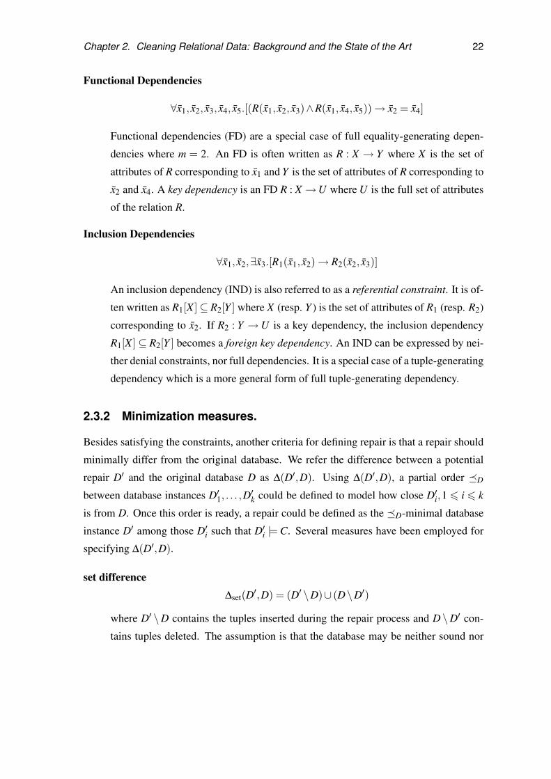
Functional Dependencies
∀x1, x2, x3, x4, x5.[(R(x1, x2, x3)∧R(x1, x4, x5))→ x2 = x4]
Functional dependencies (FD) are a special case of full equality-generating depen-
dencies where m = 2. An FD is often written as R : X → Y where X is the set of
attributes of R corresponding to x1 and Y is the set of attributes of R corresponding to
x2 and x4. A key dependency is an FD R : X →U where U is the full set of attributes
of the relation R.
Inclusion Dependencies
∀x1, x2,∃x3.[R1(x1, x2)→ R2(x2, x3)]
An inclusion dependency (IND) is also referred to as a referential constraint. It is of-
ten written as R1[X ]⊆ R2[Y ] where X (resp. Y ) is the set of attributes of R1 (resp. R2)
corresponding to x2. If R2 : Y →U is a key dependency, the inclusion dependency
R1[X ]⊆ R2[Y ] becomes a foreign key dependency. An IND can be expressed by nei-
ther denial constraints, nor full dependencies. It is a special case of a tuple-generating
dependency which is a more general form of full tuple-generating dependency.
2.3.2 Minimization measures.
Besides satisfying the constraints, another criteria for defining repair is that a repair should
minimally differ from the original database. We refer the difference between a potential
repair D′ and the original database D as ∆(D′,D). Using ∆(D′,D), a partial order �D
between database instances D′1, . . . ,D′k could be defined to model how close D′i,1 6 i 6 k
is from D. Once this order is ready, a repair could be defined as the �D-minimal database
instance D′ among those D′i such that D′i |= C. Several measures have been employed for
specifying ∆(D′,D).
set difference∆set(D′,D) = (D′ \D)∪ (D\D′)
where D′ \D contains the tuples inserted during the repair process and D \D′ con-
tains tuples deleted. The assumption is that the database may be neither sound nor

Chapter 2. Cleaning Relational Data: Background and the State of the Art 23
complete. If the database is assumed to be inconsistent but complete, no tuple inser-
tions need to be considered. In that case this symmetric set difference measure can
be simplified as asymmetric set difference:
∆aset(D′,D) = (D\D′)
cardinality of set difference
∆card(D′,D) = |(D′ \D)∪ (D\D′)|
Instead of using the set difference itself, the cardinality of set difference can also be
used to measure the difference.
number of value changes
∆change(D′(t),D(t)) = ∑A∈attr(Ri)
diffcountt,A
diffcountt,A =
{1 : D′(t,A) 6= D(t,A)
0 : D′(t,A) = D(t,A)
where attr(Ri) denotes the attributes of relation schema Ri. ∆(D′,D) is defined by
summing up ∆(D′(t),D(t)) for all the tuples in each relation of the database.
weighted distance of values
∆dis(D′(t),D(t)) = wt · ∑A∈attr(Ri)
wA ·dis(D′(t,A),D(t,A))
where dis(·) is a distance function, wt and wA are weights optionally associated with
tuple t and attribute A, respectively. Different distance functions and weights have
been used in prior work. [BBFL05, LB07b] use L1 and L2 distances of numerical
values and attribute weight. [BFFR05] uses edit distance of string values and tuple
weight.
The set measure and numerical measure require different order �D:
set inclusion based partial order
D′1 �D D′2 ⇐⇒ ∆(D′1,D)⊆ ∆(D′2,D)
When ∆(D′,D) is measured by set difference (∆set,∆aset), this order is used.

Chapter 2. Cleaning Relational Data: Background and the State of the Art 24
number comparison based total order
D′1 �D D′2 ⇐⇒ ∆(D′1,D) 6 ∆(D′2,D)
All other measures defined above (∆card,∆change,∆dis) use this order.
Different choices of ∆(D′,D) lead to different repair semantics. For example, under
asymmetric set difference minimization measure, a repair D′ is a maximal subset of D
such that D′ |= C; while under cardinality of set difference measure, such a D′ may not
be a repair: there might be a D′1, such that D′1 |= C and ∆card(D′1,D) < ∆card(D′,D), i.e.
|∆aset(D′1,D)| < |∆aset(D′,D)| although ∆aset(D′1,D) 6⊂ ∆aset(D′,D). Under both measures,
repairs need not be unique. The minimization measures have direct impact on repair opera-
tions. In the repairs defined by the first two measures (∆set,∆card), the minimal modification
unit is usually a tuple. Furthermore, for asymmetric set difference based repairs, only tuple
deletion is needed. Thus, the work using the first two measures often adopts tuple-based re-
pair semantics. However, for the last two minimization measures (∆change,∆dis), tuple level
repair operations are not enough to produce all repairs — attribute level repair operations
are needed. Consequently, the data cleaning work using these minimization measures often
takes value modification (tuple update) as its repair operation, which causes attribute-based
repair semantics.
2.3.3 Query-oriented data cleaning: consistent query answering
Consistent query answering is one of the most investigated areas closely related to data
cleaning. It is an approach to query inconsistent databases without explicitly repairing them
first. Strictly speaking, consistent query answering is not data cleaning — the database is
not physically cleaned, but kept to be inconsistent. On the other hand, consistent query an-
swering overlaps with data cleaning — the database is virtually cleaned when user queries
are answered. So the notion of repair is also needed in consistent query answering and the
same concept is shared between both of them.
A consistent answer to a query over an inconsistent database is an answer that is in-
variant under all minimal restorations of consistency to the original database [ABC99]:

Chapter 2. Cleaning Relational Data: Background and the State of the Art 25
A tuple t is a consistent answer to a query Q over a database instance D with a set of
constraints C if and only if t is an answer to the query Q over every repair D′ of D with
respect to constraints C.
In principle, to provide users with consistent query answers, the constraints need to be
associated with either the inconsistent database or the user query. As a result, there are
two flavors of consistent query answering: the database patching strategy (the constraints
are associated with the database) or the query transformation strategy (the constraints are
associated with the query).
Query Transformation Strategy. In the query transformation strategy, the inconsistent
database is unchanged. Instead, the query Q is transformed into another form to incorpo-
rate the integrity constraints. In prior work, two types of the transformed form have been
investigated. If the transformed form is in first-order, it can be easily formulated as an SQL
query Q′ and evaluated on any relational database system. This approach is referred to as
first-order rewriting. Otherwise, the transformed form could be formulated as a disjunctive
logic program P′. The final result is obtained by computing the stable models of the logic
program P′, i.e., the facts which are members of every answer set of P′. In both cases,
the result obtained from the inconsistent database is equivalent to the intersection of the
answers to the original query Q on all minimally repaired databases.
[ABC99, FM05] propose algorithms for consistent query answering under the sym-
metric set difference semantics by adopting first-order rewriting strategy. [ABC99] devel-
ops rewriting techniques for quantifier-free conjunctive queries in the presence of binary
acyclic universal integrity constraints. In brief, query Q is expanded by new conditions to
enforce the constraints C. These conditions, referred to as residues, are produced repeat-
edly by resolving literals in the possibly expanded query with constraints C. The process
continues until no more changes occur. [FM05] proposes a rewriting algorithm for a large
subset of conjunctive queries with existential quantification in the presence of primary key
constraints. The subset is defined in terms of join graph: a directed graph with its ver-
tices corresponding to the literals of the query and its arcs corresponding to each join in
the query that involves some variables that are at the position of a non-key attribute. The
algorithm runs in polynomial time in the size of the query. It works for conjunctive queries
without repeated relation symbols whose join graph is a forest. [GLRR05] further gen-
Chapter 2. Cleaning Relational Data: Background and the State of the Art 26
eralize this technique to cope with exclusion dependencies. Two prototype systems using
first-order query rewriting have been reported. [CB00] presents a system built on top of the
XSB deductive database system [SSW94] following the method in [ABC99]. [FFM05]
describes the ConQuer system based on the algorithms developed in [FM05].
The advantage of the first-order rewriting approach is that the construction of all re-
pairs is entirely avoided. This is important especially for the set difference semantics which
could potentially leads to large number of repairs. For example, in the worst case, exponen-
tial number of repairs may exists for a database with key dependencies [ABC+03c]. More-
over, the rewritten query Q′ can be expressed in SQL and therefore efficiently evaluated by
any database management system without modification. Since the rewriting is not depen-
dent on the database instance, it does not affect the data complexity of the overall consistent
query answering. Thus, as long as query Q is first-order rewritable, we can always obtain
a polynomial time (data complexity) solution for consistent query answering. However,
only restricted classes of queries are first order rewritable. Even for constraints as limited
as primary keys, [FM05] shows consistent query answering is coNP-complete for every
query of a class whose join graph is not a forest and some conjunctive queries fall into that
class. For larger constraints such as functional dependencies or denial constraints, existing
first-order rewriting algorithms can only deal with quantifier-free conjunctive queries.
In light of the limitation of first-order query rewriting, techniques for query transforma-
tion based on logic programs have been developed. [ABC03b, GGZ03] capture all repairs
of a database under the set difference semantics as answer sets of logic programs with nega-
tion and disjunction. Queries are then incorporated into these logic programs. In contrast
to first-order rewriting scenario where relational database systems are used for evaluating
Q′, here consistent query answering has to be implemented using a disjunctive logic pro-
gramming system such as DLV ([LPF+06]). This approach can handle arbitrary universal
constraints and first order queries. However, the problem of deciding whether an atom is
a member of all answer sets of a disjunctive logic program is Πp2-complete [DEGV01].
Therefore, a direct implementation of consistent query answering using disjunctive logic
programming systems is practical only for very small databases [Cho07].
Database Patching Strategy. In contrast to query transformation where the database in-
stance is involved in cleaning process as late as possible, the database patching strategy is

Chapter 2. Cleaning Relational Data: Background and the State of the Art 27
an eager approach. The inconsistent database is amended by some auxiliary structures to
incorporate the restrictions posed by the constraints. For instance, these auxiliary structures
could be a compact representation of all possible repairs with respect to the constraints.
Then the query is evaluated over the database and these auxiliary structures to get consis-
tent answers.
[ABC01, ABC+03c, CMS04, CM05, Wij05] follow the database patching strategy.
[ABC01, ABC+03c, CMS04, CM05] use graph, called conflict (hyper)graph to represent
possible repairs, while [Wij05] uses tableau, called nucleus to help compute consistent an-
swers. A conflict graph [ABC01, ABC+03c] can represent all possible repairs under func-
tional dependencies. It is an undirected graph with its vertices corresponding to the set of
tuples in the database and each edge indicating two tuples connected by the edge have con-
flicts. Conflict graph is generalized as conflict hypergraph in [CMS04, CM05] to represent
database repairs under denial constraints. The size of the conflict (hyper)graph is polyno-
mial with respect to the number of tuples in the database instance. In conflict (hyper)graph,
each repair corresponds to a maximal independent set. Based on this repair representation,
polynomial algorithms have been proposed by [CMS04, CM05] to answer quantifier-free
first-order queries with denial constraints under the asymmetric set difference semantics,
and also by [ABC01, ABC+03c] to answer group-by-free scalar aggregation queries such
as min, max, count(*), sum and avg with at most one nontrivial functional dependency
under the symmetric set difference semantics. A nucleus is a tableau where the attributes
in a tuple can take not only constants but also variables as their values. [Wij05] shows
quantifier-free conjunctive queries can be answered by nucleus in polynomial time with
respect to key dependencies or contradiction-generating dependencies. A prototype system
called Hippo has been built on top of PostgreSQL based on conflict hypergraphs [CMS04].
Similar as first-order query rewriting, these algorithms can not deal with unrestricted
conjunctive queries efficiently. In fact, it has been shown that for conjunctive queries and
constraints as restricted as primary key dependencies, consistent query answering is coNP-
complete under the asymmetric set difference semantics [CM05] and under the symmetric
set difference semantics [CLR03]. It is PNP(log(n))-complete for ground atomic queries and
denial constraints under the cardinality of set difference semantics [LB07a], while the same
problem has polynomial time complexity under the set difference semantics [CM05]. More
information on consistent query answering can be found in surveys [BC03, Ber06, Cho06,

Chapter 2. Cleaning Relational Data: Background and the State of the Art 28
Cho07].
2.3.4 Repair-oriented data cleaning: constraint repair
The repair-oriented data cleaning is also referred to as constraint repair [BFFR05] or
database fix [LB07b]. In contrast with consistent query answering, little work has been
published for repair-oriented data cleaning. The challenges and techniques are quite dif-
ferent between query and repair-oriented data cleaning although they share some common
concepts.
Minimization Measure. The minimization measure in repair-oriented data cleaning is of-
ten more selective than that in query-oriented data cleaning. The reason is that in the latter
no specific repair needs to be identified. It is not a problem if there are thousands of repairs
for a single inconsistent database as long as consistent answers can be computed for user
queries. But in the former, a specific repair needs to be singled out as the materialized fix
to the inconsistent database. If there are too many legal repairs, the choice of the final fix
could be arbitrary, which is not desired. For example, as we have seen before, the tuple
based set difference semantics have been adopted by most of the work for consistent query
answering. However, it is known that even in the presence of one functional dependency
there may be exponentially many repairs. With only 80 tuples involved in conflicts, the
number of repairs may exceed 1012 [ABC+03c, CMS04]. The cardinality of set differ-
ence minimization measure is more selective than set difference measure: every repair in
the former is also repair in the latter, but not necessarily the other way around. The most
selective measures are distance based measures presented in 2.3.2. Consequently, most
repair oriented data cleaning frameworks adopt attribute based semantics, particularly dis-
tance based minimization measures, in contrast to the prevalence of tuple based semantics
in consistent query answering context.
Repair Operations. The selective minimization measure has effects on repair operations
— it paves the way for fine-grained repair operations. We are not aware of any work in
constraint repair adopts tuple deletion/insertion as repair operations which are popular in
consistent query answering. Instead, value modification is used as the repair operation.
Such fine-grained repair operation has the advantage of losing less information than those
coarse-grained repair operations. In tuple-based repair, if a tuple is identified as dirty, all

Chapter 2. Cleaning Relational Data: Background and the State of the Art 29
values in the tuple are deleted. In fact, there might be only one dirty attribute. This whole
tuple deletion causes the loss of all useful information in those clean attributes in the tuple.
In contrast, when value modification is used to produce a repair, clean attributes are not
affected by the repair operation. Moreover, the modification is guided by the minimization
measure. The combined effects of the selective minimization measure and fine-grained
repair operation are that the modified value would be as close as possible to the original
value under the chosen distance measure. Thus the correct information in the original
inconsistent database is maximally preserved, which is one of the primary goal of data
cleaning.
[BFFR05] presents a heuristic algorithm for repairing inconsistencies based on standard
functional dependencies and inclusion dependencies. The algorithm is based on merging
equivalence classes. The minimization measure is the aggregation of edit distance of string
values between the candidate repair and the original database with considerations of tuple
weights. These weights are used to model the confidence on the original tuple. [LB07b]
develops an efficient approximation algorithm to physically repair databases which is in-
consistent in presence of denial constraints by updating numerical values. The minimiza-
tion measure is L1 distance (city distance) of numerical values with considerations of at-
tribute weights. In both scenarios, the problem of determining if there is a repair at a
distance smaller than a given value to the original database is NP-hard (in the former, it is
shown to be NP-complete). [FPL+01] uses disjunctive logic programming to repair census
data which is inconsistent with respect to first-order logic. In contrast with [LB07b] and
[BFFR05], the minimization measure is the number of value changes, which is indepen-
dent of the corrected values. Obviously, there could be large amount of repairs under this
measure. So another measure, the number of satisfied preference rules, is used to further
restrict the minimal repairs. Like consistent query answering based on logic programs, the
constraint repair system in [FPL+01] is implemented on disjunctive logic programming
system DLV ([LPF+06]).
In summary, a number of techniques have been studied for consistent query answering
and constraint repair. For the former, besides the computational complexity analysis, the
focus has been identifying and finding efficient algorithms for tractable cases and proposing
general solutions for intractable cases applicable to small data sets; for the latter, the focus
has been developing approximation or heuristic algorithms to deal with the intractability.

Chapter 2. Cleaning Relational Data: Background and the State of the Art 30
Most of the work on consistent query answering adopts the tuple based semantics such
as set difference or cardinality of set difference and deal with potentially huge number of
repairs; while the work on constraint repair uses the attribute based semantics and allows
only a few or even unique repairs.
2.4 Edit-based data cleaning: statistical data editing and
imputation
Besides the work on constraint-based data cleaning conducted in the database research
community, the problem of automatic correcting inconsistent values and filling missing
values in survey data, which is referred to as statistical data editing and imputation, has
long been investigated by statisticians. The solutions of the imputation problem are very
close to constraint-based data cleaning in spirits.
The data quality problem has long been recognized by the statisticians. The large vol-
ume of census data may contain lots of errors and must be cleaned before any statistical
analysis. This cleaning process consists of procedures to repair self-contradictory data and
fill in missing data. Before 1950s, this work had been primarily done by manual review.
Later the census data was often cleaned by a lot of if-then-else rules which are hard-wired
in a program specifically built to clean the data. However, these tools are not reusable.
Each time a new survey form is used, a new tool needs to be developed from scratch. To
further reduce human efforts, statisticians make the if-then-else rules re-configurable by
putting them in a database and reuse the data editing tool each time a new form is used —
only the rules in the database need to be updated. Not surprisingly, this leads to similar
models as constraints-based data cleaning.
The theoretical basis for a general data editing system, often called Fellegi-Holt model,
is provided in [FH76]. Under Fellegi-Holt model, the data to be cleaned is a sequence of
records. Each record contains a set of values which are encoded answers to a questionnaire.
The inconsistencies in the data are captured as a subset of the total code space that is
unacceptable. This subset is modeled by a set of rules, referred to as edits.
Data Edits. A statistical data collection could be defined in database terms as a relation.
Each tuple t in the relation corresponds to a record. Each attribute A in the schema R of

Chapter 2. Cleaning Relational Data: Background and the State of the Art 31
the relation corresponds to a field (a.k.a. a variable) in the encoded questionnaire. More
specifically, a record schema is a set of fields: R = (A1, . . . ,An) and a record instance is a
set of values t = (v1, . . . ,vn). Each field Ai takes either a numerical value that answers a
question or a categorical value that encodes the answer to a question. For instance, (8, 1, 2)
is a record instance with schema (Age, Gender, MaritalStatus). The record represents a
person who is eight years old (Age = 8), male (Gender = 1, where 1 encodes “male”, 2
encodes “female” ) and married (MaritalStatus = 2, where 1 encodes “single”, 2 encodes
“married” and 3 encodes “divorced”). For convenience, from now on, we will write a
record instance as un-encoded form such as (8, male, married). Obviously, there are errors
in this record: an eight years old boy can not be married.
All valid values of Ai form the domain of Ai, referred to as dom(Ai). Each record takes
values in the product space of these domains dom(A1)×·· ·×dom(An). This product space
could be divided into two subset: the one that contains valid combination of values of a
record and the other that contains invalid combination of values of a record. A multi-field
edit is a rule to characterize the latter subset. It catches a record in which each vaule is
valid itself, but their combination is invalid. An example multi-field edit to catch the above
error is e1 = {age<15, , married} which indicates no matter what value the Gender field
takes, being younger than 15 years old is incompatible with being married. A single-field
edit is analogous to domain constraints in database systems. It specifies a record has an
“out-of-domain” value. An example single-field edit is e2 = {age>150, , } which indicates
the age of a person should not be larger than 150.
An edit is either a single-field edit or a multi-field edit. A set of edits E could be defined
by domain experts for a collection of records. The edits serve the opposite purpose as con-
strains C in constraint-based data cleaning: edits express error condition, i.e. characterize
dirty data, while constraints are used to model clean data. A record failing any edit in E is
regarded as an inconsistent record and thus needs to be corrected. A consistent record is
the one that passes (i.e., succeeds, or satisfies) all the edits.
Record Correction. An edit-based data cleaning model is defined as below:

Chapter 2. Cleaning Relational Data: Background and the State of the Art 32
An edit-based data cleaning model consists a collection of records D to be cleaned and
a set E of edits to capture errors in D. A record t in D is dirty if it fails any edit in E.
A correction of a dirty record t is specified as a consistent record t ′ derived from t such
that (1) t ′ passes all edits in E; (2) fewest number of fields in t has been changed; and (3)
the original joint frequency distributions of the data is preserved as far as possible. Dataediting and imputation is the process of using edit rules to identify errors in records
and find their corrections.
A correction for a collection of records is analogous to a repair in constraint-based
data cleaning; the data editing and imputation is analogous to constraint repair. Similar to
constraint-based data cleaning, the correction needs to satisfy all of the rules and respect
the minimal change principle. Here, the minimization measure is the number of values
changed. An additional requirement, which is not needed in constraint-based data cleaning,
is the preservation of joint frequency distribution. This is needed to prevent the statistics of
the data from being affected by the correction.
Error Detection. A merit of Fellegi-Holt model is that, in one pass through the data, for
an edit-failing record, a minimal set of fields can be found. If these fields are changed it
is guaranteed to yield a correction. The process of finding such a minimal set of fields is
referred to as error localization. It is analogous to the error detection in constraint-based
data cleaning. A difference is that in the latter only inconsistencies are detected, the er-
roneous values are not further identified among the inconsistent data. [FH76] has proven
that one way to solve the error localization problem is to compute a complete set of edits
— including both the edits explicitly specified by users and some implicit edits logically
derived from the explicit ones. The process of deriving implicit edits is referred to as edit
generation and the required implicit edits in error localization are referred to as essentially
new edits in [FH76]. Although the guarantee of finding a correction by changing minimal
set of fields is appealing, both edit generation and error localization are computationally
intractable [GKL86]. To overcome these bottlenecks, a number of algorithms are proposed
to speed up their computations. [GKL86, Win95, Win97, Che98] develop different alter-
natives of edit generation and error localization algorithms.
Edit Generation Unlike error localization which has to be computed in the cleaning pro-
cess, edit generation could be precomputed because the record instance is not needed in the

Chapter 2. Cleaning Relational Data: Background and the State of the Art 33
computation. Some literature views edit generation as a pre-processing step for error local-
ization [GKL86, Win95, Win97]. [GKL86] re-defines the complete set of edits in [FH76]
as the original explicit edits plus the set of maximal implicit edits. By adopting maximal
implicit edits, it removes the redundant edits which are not maximal, i.e. any edit that is
properly included in another edit. It shows the re-defined complete edits are sufficient for
solving the error localization problem and proposes an algorithm which is computation-
ally superior to that of [FH76] for generating these edits. [Win95] observes that the edit
generation algorithm in [GKL86] may fail in some situation and presents an alternative
one, called EG algorithm, to correctly generates all maximal implicit edits. [Win97] uses
a heuristic, called EGE algorithm, to reduce the computation at nonroot generating fields.
It is much faster than EG algorithm and generates most of the implicit edits. [Che98] fur-
ther improves the performance by only finding all prime cover solutions of the set covering
problem which is needed in generating edits.
Edit Validation Another virtue of Fellegi-Holt model is that, prior to the receipt of data
records, the mutual consistency of the explicit edits could be checked in the edit generation
process. Thus, as a side effect, the edit generation also solves the edit validation problem
which is in analogous to the consistency checking of constraints in a constraint-based data
cleaning system.
Error Localization If the implicit edits are generated prior to editing, the amount of
computation needed for error localization can be significantly reduced [Win99]. How-
ever, the generation of a complete set of edits often requires days-to-months of computa-
tion [Gar03, Win99]. Thus some approaches directly solve the error localization problem
without computing implicit edits [San79, KMW88, dW96] or compute partial implicit edits
on-the-fly [DW97]. However, In the latter, it is not guaranteed to find a solution for error
localization. In the former, there is no control over how long it will take for a record. Those
approaches usually introduce time-out mechanism to skip a record if it takes too much time.
These records need to be manually inspected and corrected.
Relations to Logic. [BS01, BGH03] have shown the edits in Fellegi-Holt model could
be expressed in propositional logic and the edit validation could be achieved by solving a
sequence of Satisfiability problem, the edit generation is essentially the same as a technique
for automating logical deduction called resolution.

Chapter 2. Cleaning Relational Data: Background and the State of the Art 34
The theories, algorithms developed for statistical editing and imputation problem have
provided important solutions for rule-based data cleaning, in particular in the case where
the set of rules are not large. In practical case, however, such methods suffer from severe
computational limitations [Win99]. According to [Win99], it is unlikely that current algo-
rithms can generate the full set of implicit edits with 300 explicit edits, while as many as
750 explicit edits may be needed by a large survey form or in complicated edit situations.
In addition to this limitation on the size of the rules, the edits only express single-record
(single-field or multiple-field) constraints that are commonly encountered in survey data.
However, in a database context, the inconsistencies may arise due to relationship between
tuples (functional dependencies) or between relations (inclusion dependencies). There is
no efficient way to translate these constraints into small number of edits.
2.5 Beyond rule-based data cleaning
There are also work in which the dirty data is not captured by rules. One line of research
is to identify errors as outliers and remove them. Another one is using data mining tech-
niques to explain the data quality problem and suggest corrections of the errors — instead
of removing them. In the first line of research, [Joh95] extends the pruning scheme in
C4.5, a decision tree algorithm, to fully remove the effect of outliers. [AAR96] presents a
linear algorithm to find deviations in large databases by simulating a mechanism familiar to
human beings: after seeing a series of similar data, an element disturbing the series is con-
sidered as a possible error. A dissimilarity function is proposed to capture how dissimilar
a new data item is from the data items seen so far. In the second line of research, [SW00]
uses Bayesian techniques to detect and correct dirty data by taking advantage of depen-
dencies between attributes and exploiting expert knowledge of the relationships among the
attributes. [KM03] provides an algorithm for the unsupervised discovery of three proba-
bilistic models: a generative model of the clean records, a generative model of the noise
values, and a probabilistic model of the corruption process. These models are used to assist
detecting and correcting dirty data. More methods are surveyed in [MM00].
In above approaches, whether the outliers or noises are errors or not depends on the
domain. Sometimes, these outliers might be correct data that do not fit the clean model.
Therefore, the correction of outliers should always be assisted by domain experts [LGJ03].
Chapter 2. Cleaning Relational Data: Background and the State of the Art 35
This non-deterministic nature limits their uses as independent automatic data cleaning
tools. These methods are often used to assist semi-automatic cleaning of data.
2.6 Summary
In this chapter, the work on rule-based data cleaning is summarised. Most of the existing
work is focusing on consistent query answering and statistical data editing and imputation
problems. Little work has been done on constraint repair.
There are many scenarios where constraint repair is preferred than consistent query
answering. In consistent query answering, most of the cleaning computations are pushed
to query answering stage. In constraint repair, the the cleaning computations are conducted
at repairing stage; the query answering needs no special treatment — any DBMS can be
used for its query evaluation. In reality, users are more tolerant with repairing than query
answering in terms of time: they usually expect prompt answers to their queries; while
they can wait for hours or even days for repairing the dirty data through a batch processing
operation. Even when eager approaches (database patching strategy) are used in consistent
query answering, performance issue still exists: the evaluation of queries can not take
advantages of the well developed database index and optimization techniques because the
compact representation of repairs is not stored as normal database tables. Moreover, when
the data set is not frequently changed or read only, a physical repair ispreferredd because the
same copy of repaired data could be used repeatedly to answer querieswithoutt new effort
unless the data is updated. In data mining or data warehousing projects where data quality
is a severe problem, complex computations need to be conducted on large set of data. As
explained earlier, consistent query answering can hardly support complex queries and large
set of data as the same time. Besides the performance concern, in many applications such
as data exchange, the users need a physically repaired database.
On the other hand, although the solutions for statistical data editing and imputation
can be used to obtain physicrepairsirs of inconsistent data, those solutions are tailored for
census/survey data where inconsistencies mostly occur inside a record (tuple) and the major
concern for choosing corrections (repair) is not to destroy the statistics. Little work has
been done to adapt those solutions to constraint repair.
In constraint repair, functional/inclusion dependencies [BFFR05], denial con-

Chapter 2. Cleaning Relational Data: Background and the State of the Art 36
straints [LB07b] and first order logic [FPL+01] have been studied for characterizing the
data. Their focus is the developing of accurate and efficient repairing algorithms. No work
has been done to tailor (extend or restrict) traditional constraints in data cleaning context.
In the next two chapters of the thesis, a novel extension of functional dependencies is pro-
posed for repair-oriented data cleaning. Efficient algorithms for detecting and repairing
inconsistencies in data are presented.

Chapter 3
Modeling the Consistency of Data
One of the most important questions in connection with data cleaning is how to model the
consistency of the data, i.e. how to specify and determine that the data is clean? This calls
for appropriate application-specific integrity constraints [RD00] to model the fundamental
semantics of the data.
As summarized in the last chapter, recent work on data cleaning specifies the consis-
tency of data in terms of constraints, and detects inconsistencies in the data as violations of
the constraints. However, previous work on constraint repair is mostly based on traditional
dependencies (e.g. functional and full dependencies, etc), which were developed mainly for
schema design, but are often insufficient to capture the semantics of the data, as illustrated
by the example below.
Example 3.1: A company maintains a relation of customer records:
customer (NAME, CNT, CITY, STR, ZIP, CC, AC, PN).
Each customer tuple contains the NAME, address (country CNT, city CITY, street STR,
postal code ZIP) and phone information (country code CC, area code AC, phone number
PN) of a customer.
Traditional functional dependencies (FDs) on a customer relation may include:
f1: [CC, AC, PN ]→ [STR, ZIP, CNT ]
f2: [CNT, ZIP ]→ [CITY ]
37
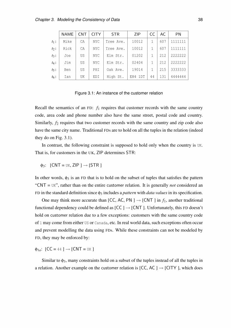
Chapter 3. Modeling the Consistency of Data 38
NAME CNT CITY STR ZIP CC AC PN
t1: Mike CA NYC Tree Ave. 10012 1 607 1111111
t2: Rick CA NYC Tree Ave. 10012 1 607 1111111
t3: Joe US NYC Elm Str. 01202 1 212 2222222
t4: Jim US NYC Elm Str. 02404 1 212 2222222
t5: Ben US PHI Oak Ave. 19014 1 215 3333333
t6: Ian UK EDI High St. EH4 1DT 44 131 4444444
Figure 3.1: An instance of the customer relation
Recall the semantics of an FD: f1 requires that customer records with the same country
code, area code and phone number also have the same street, postal code and country.
Similarly, f2 requires that two customer records with the same country and zip code also
have the same city name. Traditional FDs are to hold on all the tuples in the relation (indeed
they do on Fig. 3.1).
In contrast, the following constraint is supposed to hold only when the country is UK.
That is, for customers in the UK, ZIP determines STR:
φ3: [CNT = UK, ZIP ]→ [STR ]
In other words, φ3 is an FD that is to hold on the subset of tuples that satisfies the pattern
“CNT = UK”, rather than on the entire customer relation. It is generally not considered an
FD in the standard definition since φ3 includes a pattern with data values in its specification.
One may think more accurate than [CC, AC, PN ]→ [CNT ] in f1, another traditional
functional dependency could be defined as [CC ]→ [CNT ]. Unfortunately, this FD doesn’t
hold on customer relation due to a few exceptions: customers with the same country code
of 1 may come from either US or Canada, etc. In real world data, such exceptions often occur
and prevent modelling the data using FDs. While these constraints can not be modeled by
FD, they may be enforced by:
φ1a: [CC = 44 ]→ [CNT = UK ]
Similar to φ3, many constraints hold on a subset of the tuples instead of all the tuples in
a relation. Another example on the customer relation is [CC, AC ]→ [CITY ], which does

Chapter 3. Modeling the Consistency of Data 39
not hold in US (e.g., for area code 610, the city could be Allentown, Bethlehem, etc.), but
holds in UK, China and most other countries:
φ4a: [CC = 44, AC ]→ [CITY ]
In US, although it doesn’t hold in general, it still holds for some area codes:
φ4b: [CC = 1, AC = 212 ]→ [CITY = NYC ]
φ4c: [CC = 1, AC = 215 ]→ [CITY = PHI ]
The following constraints are again not considered FDs:
φ1b: [CC = 1, AC = 607, PN ]→ [STR, ZIP, CNT = US ]
φ2a: [CNT = US, ZIP = 10012 ]→ [CITY = NYC ]
φ2b: [CNT = US, ZIP = 19014 ]→ [CITY = PHI ]
The first constraint φ1b assures that only for country code 1 and area code 607, if two tuples
have the same PN, then they must have the same STR and ZIP values and furthermore, the
country must be US. Similarly, φ2a specifies that for all tuples in the us and with zip code
10012, their city must be NYC (irrespective of the values of the other attributes); and φ2b
assures that if the zip code is 19014 then the city must be PHI.
Observe that φ1b refine the standard FD f1 given above, while φ2a and φ2b refines the FD
f2. This refinement essentially enforces a binding of semantically related data values. Note
that while tuples t1 and t2 in Fig. 3.1 do not violate f1, they violate its refined version φ1,
since the country cannot be CA if the country code and area code are 1 and 607, respectively.
2
In this example, the constraints φ1a,b,φ2a,b,φ3,φ4a,b,c capture a fundamental part of the
semantics of the data. However, they cannot be expressed as standard FDs and are not
considered in previous work on data cleaning. Constraints that hold conditionally may arise
in a number of domains. For example, an employee’s pay grade may determine her title
in some parts of an organization but not in others; an individual’s address may determine
his tax rate in some countries while in others it may depend on his salary, etc. Further,
dependencies that apply conditionally appear to be particularly needed when integrating
data, since dependencies that hold only in a subset of sources will hold only conditionally
in the integrated data. These call for the study of conditional dependencies, which aim to

Chapter 3. Modeling the Consistency of Data 40
capture data inconsistencies at the intentional level (as done in prior work on data cleaning)
and extensional level in a uniform framework.
In response to the practical need for such constraints, a novel extension of traditional
FDs is introduced in next section, referred to as conditional functional dependencies (CFDs),
that are capable of capturing the notion of “correct data” in these situations. A CFD extends
an FD by incorporating a pattern tableau that enforce binding of semantically related values.
Unlike its traditional counterpart, the CFD is required to hold only on tuples that satisfy a
pattern in the pattern tableau, rather than on the entire relation. For examples, all the
constraints we have encountered so far can be expressed as CFDs.
3.1 Conditional Functional Dependencies
In this section we define conditional functional dependencies (CFDs). Consider a relation
schema R defined over a fixed set of attributes, denoted by attr(R).
Syntax. A CFD ϕ on R is a pair (R : X → Y, Tp), where (1) X ,Y are sets of attributes from
attr(R), (2) R : X → Y is a standard FD, referred to as the FD embedded in ϕ; and (3) Tp is
a tableau with all attributes in X and Y , referred to as the pattern tableau of ϕ, where for
each A in X or Y and each tuple t ∈ Tp, t[A] is either a constant ‘a’ in the domain dom(A)
of A, or an unnamed variable ‘ ’.
If A occurs in both X and Y , we use t[AL] and t[AR] to indicate the occurrence of A in
X and Y , respectively, and separate the X and Y attributes in a pattern tuple with ‘‖’. We
write ϕ as (X → Y, Tp) when R is clear from the context.
Example 3.2: The constraints φ1a,b,φ2a,b,φ3, φ4a,b,c on the customer table given in Exam-
ple 3.1 can be expressed as CFDs ϕ1 (for φ1a and φ1b, from the second line one per line,
respectively), ϕ2 (for φ2a and φ2b), ϕ3 (for φ3), and ϕ4 (for φ4a,φ4b, and φ4c, one per line),
as shown in Fig. 3.2. In fact all the constraints we have encountered so far can be expressed
as CFDs. Indeed, the traditional functional dependencies f1 and f2 are expressed by the first
pattern tuple of CFDs ϕ1 and ϕ2 given in Fig. 3.2, respectively. 2
If we represent both data and constraints in a uniform tableau format, then at one end
of the spectrum are relational tables which consist of data values without logic variables,
and at the other end are traditional constraints which are defined in terms of logic variables

Chapter 3. Modeling the Consistency of Data 41
T1 =
CC AC PN STR ZIP CNT
44 UK
1 607 US
(a) ϕ1 = ([CC, AC, PN ]→ [STR, ZIP, CNT ], T1)
T2 =
CNT ZIP CITY
US 10012 NYC
US 19014 PHI
(b) ϕ2 = ([CNT, ZIP ]→ [CITY ], T2)
T4 =
CC AC CITY
44
1 212 NYC
1 215 PHI
(c) ϕ4 = ([CC, AC ]→ [CITY ], T4)
T3 =CNT ZIP STR
UK
(d) ϕ3 = ([CNT, ZIP ]→ [STR ], T3)
Figure 3.2: Example CFDs
but without data values, while CFDs are in the between.
Semantics. Intuitively, the pattern tableau Tp of ϕ refines the standard FD embedded in ϕ
by enforcing the binding of semantically related data values. To define the semantics of ϕ,
we first introduce a notation. For a pattern tuple tp in Tp, we define an instantiation ρ to be a
mapping from tp to a data tuple with no variables, such that for each attribute A in X ∪Y , if
tp[A] is ‘ ’, ρ maps it to a constant in dom(A), and if tp[A] is a constant ‘a’, ρ maps it to the
same value ‘a’. For example, for tp[A,B] = (a, ), one can define an instantiation ρ such that
ρ(tp[A,B]) = (a,b), which maps tp[A] to itself and tp[B] to a value b in dom(B). Obviously,
for an attribute A occurring in both X and Y , we require that ρ(tp[AL]) = ρ(tp[AR]).
A data tuple t is said to match a pattern tuple tp, denoted by t � tp, if there is an
instantiation ρ such that ρ(tp) = t. For example, t[A,B] = (a,b)� tp[A,B] = (a, ).
A relation I of R satisfies the CFD ϕ, denoted by I |= ϕ, if for each pair of tuples t1, t2 in
the relation I, and for each tuple tp in the pattern tableau Tp of ϕ, if t1[X ] = t2[X ] � tp[X ],
then t1[Y ] = t2[Y ] � tp[Y ]. That is, if t1[X ] and t2[X ] are equal and in addition, they both

Chapter 3. Modeling the Consistency of Data 42
match the pattern tp[X ], then t1[Y ] and t2[Y ] must also be equal to each other and both match
the pattern tp[Y ]. Moreover, if Σ is a set of CFDs, we write I |= Σ if I |= ϕ for each CFD
ϕ ∈ Σ. If a relation I |= Σ, then we say that I is clean with respect to Σ.
Example 3.3: The customer relation in Fig. 3.1 satisfies ϕ2, ϕ3 and ϕ4 of Fig. 3.2. How-
ever, it does not satisfy ϕ1. Indeed, tuple t1 violates the pattern tuple tp = (01, 607, ‖, , US) in tableau T1 of ϕ1: t1[CC,AC,PN] = (01, 607, 1111111) � (01, 607, ), but
t1[STR,ZIP,CNT] = (Tree Ave., 07974, CA) 6� ( , , US) since t1[CNT] is CA instead of
US; similarly for t2. 2
This example tells us that while violation of a standard FD requires two tuples, a single
tuple may violate a CFD.
Two special cases of CFDs are worth mentioning. First, a standard FD X → Y can
be expressed as a CFD (X → Y, Tp) in which Tp contains a single tuple consisting of ‘ ’
only. For example, if we let T2 of ϕ2 in Fig. 3.2 contain only ( , ‖ ), then it is the
CFD representation of the FD f2 given in Example 3.1. Second, an instance-level FD X →Y studied in [LSPR96] is a special CFD (X → Y, Tp), where Tp contains a single tuple
consisting of only data values.
Observe that pattern tableaux in CFDs are quite different from Codd tables, variable
tables and conditional tables, which have been traditionally used in the context of incom-
plete information [IJ84, Gra91]. The key difference is that each of these tables represents
possibly infinitely many relation instances, one instance for each instantiation of variables.
No instance represented by these table formalisms can include two tuples that result from
different instantiations of a table tuple. In contrast, a pattern tableau is used to constrain–as
part of a CFD–a single relation instance, which can contain any number of tuples that are
all instantiations of the same pattern tuple via different valuations of the unnamed variables
‘ ’.
Normal form. From the semantics of CFDs we immediately obtain a normal form of CFDs:
Given a set Σ of CFDs, we may assume that each CFD φ ∈ Σ is of the form φ = (R : X →A, tp), where A ∈ attr(R) and tp is a single pattern tuple. For ease of exposition we assume
that CFDs are given in the normal form.
Satisfiability. To clean data based on CFDs we need to make sure that the CFDs are sat-
isfiable, or make sense. The satisfiability problem is to determine, given a set Σ of CFDs,

Chapter 3. Modeling the Consistency of Data 43
whether or not there exists a (non-empty) database D such that D |= Σ. While this problem
is trivial for traditional FDs, i.e. any set of FDs is satisfiable, this is no longer true for CFDs.
Indeed, it has been shown that this problem is intractable in general [BFG+07, FGJK08].
However, when the database schema is fixed, satisfiability of CFDs can be decided in
PTIME [BFG+07, FGJK08]. In the sequel we consider satisfiable CFDs only.
3.2 Detecting CFD Violations
A first step for data cleaning is the efficient detection of constraint violations in the data.
In this section we develop techniques to detect violations of CFDs. Given an instance I
of a relation schema R and a set Σ of CFDs on R, it is to find all the violating tuples in I,
i.e. the tuples that (perhaps together with other tuples in I) violate some CFD in Σ. We first
provide an SQL technique for finding violations of a single CFD, and then present an incre-
mental technique for validating CFDs. It is desirable to use just SQL to find violations: this
makes detection feasible in any standard relational DBMS without requiring any additional
functionality on its behalf.
3.2.1 Checking a CFD with SQL
Consider a CFD ϕ = (X → A, Tp). A naıve approach to find the tuples violating ϕ is
demonstrated by the following example:
Example 3.4: Given ϕ4 = ([CC,AC ]→ [CITY ], T4) shown in 3.2. Naıvely, we can issue
three SQL queries, one for each pattern tuple tp ∈ T4, to identity inconsistent tuples in a
customer instance:
Q1ϕ4
select distinct AC from customer t
where t[CC] =‘44’
group by AC having count (distinct CITY)> 1
Q2ϕ4
select * from customer t
where t[CC] =‘1’ and t[AC] =‘212’ and t[CITY] <>‘NYC’
Q3ϕ4
select * from customer t
where t[CC] =‘1’ and t[AC] =‘215’ and t[CITY] <>‘PHI’

Chapter 3. Modeling the Consistency of Data 44
Although each query in the above example is very efficient providing proper indice
have been created for the customer relation, the number of the queries — which equals to
the number of tuples in the pattern tableau — could be huge. Since CFD allows the binding
of values, the cardinality of a CFD could easily grow very large in practice. For example, to
achieve precise checking of the consistency between postal codes and addresses, one may
create a large pattern tableau containing all the mappings of postal codes and addresses in a
country or even for the world. Such a pattern tableau could even be larger than the database
instance.
Is there a way to detect CFD violations without using potentially large number of SQL
queries? Let’s look at a different query to find the tuples violating ϕ3 by directly following
the CFD definition:
Qϕ4 select t1.* from customer t1, customer t2, T4 tp
where t1[CC] = t2[CC]� tp[CC] and t1[AC] = t2[AC]� tp[AC]
and not (t1[CITY] = t2[CITY]� tp[CITY] )
where t1[CC] = t2[CC] � tp[CC] is a short-hand for the SQL expression (t1[CC] = t2[CC]
and (t2[CC] = tp[CC] or tp[CC] = ‘ ’)), and similarly for t1[AC] = t2[AC] � tp[AC] and
t1[CITY] = t2[CITY]� tp[CITY].
Obviously, this single query is enough to detect all the violations in a customer instance
against CFD ϕ4 irrespective to the size of the CFD, because the pattern tableau T4 is treated
as an ordinary data table. These pattern tables are dynamically created when a CFD with
a new embedded FD is specified. Since the number of pattern tuples could be larger than
the cardinality of the relation instance as explained earlier, the size of the SQL query in
the Naıve approach may exceed the relation instance. So the communication time for
sending these queries could grow as high as to transfer the relation instance, not to mention
that it is not feasible to keep the queries in memory. In other words, the Naıve approach
encodes the potential huge domain knowledge in the queries. Now the domain knowledge
is stored in the database and only a small SQL query is needed for checking CFD violations.
As a result, the communication time is reduced dramatically by the compactness of the
query. However, this compact query is very costly. The self-join of customer relation is an
expensive operation which causes the poor performance.

Chapter 3. Modeling the Consistency of Data 45
Thus, it is natural to ask if there is an approach to detect CFD violations which combines
the advantages of both methods above, i.e., an approach to compose a set of concise queries,
irrespective to the size of the CFD, that can efficiently find the inconsistent tuples in an
instance against a CFD without expensive joins?
By analyzing the above queries, we find that to achieve this goal we should: (1) separate
the detection of single-tuple violations (i.e. the tuples violating the bound values in the
pattern tableau of a CFD) and multi-tuple violations (i.e. the sets of tuples in which each
set mutually violate at least one pattern tuple with ‘ ’ at RHS); (2) favor the “group by”
operations and avoid using the self-join. 2
Follows the above guidance, we found a way to compose efficient queries to detect CFD
violations. Given a CFD ϕ = (X → A, Tp), the following two SQL queries suffice to find
the tuples violating ϕ:
QCϕ select * from R t, Tp tp
where t[X ]� tp[X ] and t[A] 6� tp[A]
QVϕ select distinct X from R t, Tp tp
where t[X ]� tp[X ] and tp[A] = ‘ ’
group by X having count (distinct A)> 1
where for an attribute B ∈ (X ∪A), t[B]� tp[B] is a short-hand for the SQL expression (t[B]
= tp[B] or tp[B] = ‘ ’), while t[B] 6� tp[B] is a short-hand for (t[B] 6= tp[B] and tp[B] 6= ‘ ’).
Intuitively, detection is a two-step process, each conducted by a query. Initially, query
QCϕ detects single-tuple violations, i.e. the tuples t in I that match some pattern tuple tp ∈ Tp
on the X attributes, but t does not match tp in A since the constant value tp[A] is different
from t[A]. That is, QCϕ finds violating tuples based on differences in the constants in the
tuples and Tp patterns.
On the other hand, query QVϕ finds multi-tuple violations, i.e. tuples t in I for which
there exists a tuple t ′ in I such that t[X ] = t ′[X ] and moreover, both t and t ′ match a pattern
tp on the X attributes, value tp[A] is a variable, but t[A] 6= t ′[A]. Query QVϕ uses the group by
clause to group tuples with the same value on X and it counts the number of distinct instan-
tiations in tp[A]. If there is more than one instantiation, then there is a violation. Note that
QVϕ returns only the X attributes of violating tuples. This has the advantage that the output

Chapter 3. Modeling the Consistency of Data 46
QCϕ1
select * from customer t, T1 tp
where t[CC]� tp[CC] and t[AC]� tp[AC] and t[PN]� tp[PN] and(t[STR] 6� tp[STR] or t[ZIP] 6� tp[ZIP] or t[CNT] 6� tp[CNT])
QVϕ1
select distinct CC,AC,PN from customer t, T1 tp
where t[CC]� tp[CC] and t[AC]� tp[AC] and t[PN]� tp[PN] and(tp[STR] = ‘ ’ or tp[ZIP] = ‘ ’ or tp[CNT] = ‘ ’)
group by CC, AC, PN having count (distinct STR, ZIP, CNT)> 1
Figure 3.3: SQL queries for checking CFD ϕ1
is more concise than when we would return the complete tuples. Moreover, the complete
tuples can be easily obtained using an additional SQL query.
This solution can be trivially extended to multiple attributes, as illustrated in the fol-
lowing example:
Example 3.5: Recall CFD ϕ1 given in Fig. 3.2. Over a customer instance I, the SQL
queries QCϕ1
and QVϕ1
shown in Fig. 3.3 determine whether or not I satisfies ϕ1. Executing
these queries over the instance of Fig. 3.1, it returns tuples t1, t2 (due to QCϕ1
), and t3 and t4(due to QV
ϕ1). 2
A salient feature of our SQL translation is that tableau Tp is treated an ordinary data
table. Therefore, each query is bounded by the size of the embedded FD X→ A in the CFD,
and is independent of the size (and contents) of the (possibly large) tableau Tp.
3.2.2 Incremental CFD Detection
Consider an instance I of a relation schema R and a CFD ϕ = (X → A, Tp). Given the
methodology presented thus far, we can check for violations of ϕ by issuing the pair of
queries QCϕ and QV
ϕ over I. An interesting questions is then what happens if the instance I
changes? As tuples are inserted or deleted from I, resulting a new instance Inew, a naive
solution would be a batch approach that re-issues queries QCϕ and QV
ϕ over Inew, starting
from scratch in response to updates, something that requires two passes of the underlying
instance each time the queries are re-issued.

Chapter 3. Modeling the Consistency of Data 47
Intuitively, however, one expects that a tuple insertion leaves a large portion of instance
I unaffected when CFD violations are concerned. An inserted tuple t might introduce new
violations, but only with tuples that are already in the instance and match t in the X at-
tributes. Therefore, it makes sense to only access these tuples and only detect the possible
newly introduced violations due to the inserted tuple. Thus, incremental detection can po-
tentially save a large number of disk accesses, since instead of performing two passes of the
underlying data on each tuple insertion (naive method), we only need to access the tuples
that match the inserted tuple t in the X attributes. Similarly in the case of deletion, by delet-
ing a tuple t we might inadvertibly repair some of the violations in I that the deleted tuple
was causing (again with tuples matching t in the X attributes). Therefore, it makes sense to
only detect which of the existing violations concerning the deleted tuple are affected. The
following example better illustrates the above.
Example 3.6: Recall from Example 3.5 that tuples t1 to t4 in Fig. 3.1 violate CFD ϕ1. Now,
consider inserting the tuple t7 : (Bill, US, PHI, Main Rd., 19014, 01, 215, 3333333)
in the relation of the figure. It is easy to check that tuples t5 and t7 violate ϕ1 (due to
QVϕ1
). Still, the newly inserted tuple does not affect the violations detected between the first
four tuples. Note that an incremental detection would require that we only access tuple t5,
instead of the whole relation.
Now, consider again the instance in Fig. 3.1 and assume that we delete tuple t4 from
it. Then, it is easy to check that tuple t3 no longer violates ϕ1 since the deletion of t4inadvertibly repaired the violation caused by tuples t3 and t4. At the same time, note that
such a deletion only requires accessing tuple t3 and does not affect the violation caused by
tuples t1 and t2. 2
We next present a method to incrementally detect CFD violations, given a set of in-
sertions and deletions to an instance I. Although the incremental method has the same
worst-case performance as the naive method (two passes of the underlying instance), its
expected performance is that only a small number of tuples are accessed, which will be
verified in the next section by our experiments.

Chapter 3. Modeling the Consistency of Data 48
NAME CNT CITY STR ZIP CC AC PN βCϕ1
βVϕ1
t1: Mike CA NYC Tree Ave. 10012 1 607 1111111 1 0
t2: Rick CA NYC Tree Ave. 10012 1 607 1111111 1 0
t3: Joe US NYC Elm Str. 01202 1 212 2222222 0 1
t4: Jim US NYC Elm Str. 02404 1 212 2222222 0 1
t5: Ben US PHI Oak Ave. 19014 1 215 3333333 0 0
t6: Ian UK EDI High St. EH4 1DT 44 131 4444444 0 0
Figure 3.4: The customer relation instance with logging information
3.2.2.1 Logging of violations
The incremental detection requires us to extend the schema R of an instance relation I to
record which tuples violate which CFDs in a given set Σ. In more detail, for each CFD ϕ∈ Σ
we add two Boolean attributes βCϕ and βV
ϕ to the schema of R. We use Rlog to denote the new
schema. For each tuple t ∈ I, we create a tuple t ′ in Rlog such that t ′[attr(R)] = t[attr(R)].
Furthermore, in attribute t ′[βCϕ] (resp. t ′[βV
ϕ ]) we record whether or not the corresponding
tuple t violates CFD ϕ due to QCϕ (resp. QV
ϕ ). Note that our logging mechanism imposes min-
imum overhead, in terms of space, since for each tuple and each CFD only two additional
bits are required.
We assume that, initially, we execute queries QCϕ and QV
ϕ and we use the result of the
two queries to initialize the values of attributes βCϕ and βV
ϕ , through a simple SQL update
statement of the following form for βCϕ (similarly for βV
ϕ ):
UCϕ update Rlog t ′ set t ′[βC
ϕ] = 1
where t ′[attr(R)] in (QCϕ)
One needs only to select all those tuples with both βCϕ and βV
ϕ equal to false, for each ϕ ∈ Σ,
and then project on attr(R), in order to retrieve from Rlog the tuples that do not violate any
of the CFDs. Figure 3.4 shows the instance of Fig. 3.1 after its schema has been extended
appropriately to log violations for CFD ϕ1.

Chapter 3. Modeling the Consistency of Data 49
3.2.2.2 Handling tuple deletions
We use SQL statements to detect violations, in an incremental fashion. Consider a CFD
ϕ = (X → A, Tp) and an instance Ilog whose schema Rlog includes attributes βCϕ and βV
ϕ .
In response to deletion of tuple t from Ilog, the incremental detection of violations has two
simple steps.
Step 1: delete from Rlog t ′ where t ′ = t
Step 2: update Rlog t ′ set t ′[βVϕ ] = 0
where t ′[βVϕ ] = 1 and t ′[X ] = t[X ] and
1 = ( select count (distinct A) from Rlog t ′′
where t ′′[X ] = t[X ])
In more detail, the SQL query in the first step simply deletes from Rlog the tuple corre-
sponding to t. The second step checks for tuples that (a) violate ϕ (t ′[βVϕ ] = 1), (b) have the
same values on the X attributes with t, and (c) all these identified tuples have the same A
attribute value. It is easy to see that if a set of tuples satisfies the above three conditions,
then each of the tuples in the set violated ϕ only due to t. Since we delete t, each of the
tuples now satisfies ϕ. Therefore, we set t ′[βVϕ ] to false. Note that a tuple deletion only
affects violations that are caused by the presence of ‘ ’ in the tableau, hence we focus only
on the βVϕ attribute. Also note that the above procedure need not access the pattern tableau
Tp of ϕ, resulting in additional savings in terms of execution time.
Example 3.7: Consider the instance in Fig. 3.4 and assume that we delete tuple t4. Then
the second step of our incremental detection will select tuple t3 and set t3[βVϕ1
] to false since
there is no other tuple in the instance that has the same values on the CC, AC and PN
attributes as t3 but differs from t3 in STR, CT or ZIP. Hence tuple t3 no longer violates ϕ1.
Note that our incremental detection, using appropriate indexes, only accesses tuple t3. In
contrast the non-incremental detection requires to access the whole relation twice. 2
An interesting question is what happens when we want to do batch deletion, i.e., delete
a set of tuples. Obviously, we could execute the above two steps once for each tuple in the
set. We can actually do better than that since it suffices to execute the above steps once for
each distinct value of X attributes that is deleted. So, if for example we delete both tuples
t3 and t4 from the instance in Fig. 3.4, we only need to execute the two steps once since

Chapter 3. Modeling the Consistency of Data 50
the two tuples have the same value on the X attributes. This simple observation provides
additional savings.
3.2.2.3 Handling tuple insertions
Assume that we want to insert a tuple t into Ilog. Then, the incremental detection of viola-
tions has the following three steps.
Step 1: insert into Rlog values t
Step 2: update Rlog t ′ set t ′[βCϕ] = 1
where t ′ = t andexists ( select * from Tp
where tp[X ]� t ′[X ] and tp[A] 6� t ′[A])
Step 3: update Rlog t ′ set t[βVϕ ] = 1, t ′[βV
ϕ ] = 1
where t ′[X ] = t[X ] and t ′[A] 6= t[A] andexists ( select * from Tp tp
where tp[X ]� t[X ] and tp[A] = ‘ ’)
The first step simply inserts the tuple t into relation Rlog, where we assume that both the
βCϕ and βV
ϕ attributes are set to false, for each newly inserted tuple. Similar to QCϕ, the
second step checks for violations in the constants between the recently inserted tuple and
the pattern tableau Tp. If such violations exist, it sets the value of βCϕ in the inserted tuple
to true. Similar to QVϕ , the final step checks for tuples that (a) have the same values on the
X attributes with t, (b) differ from t on the A attribute, and (c) the pattern tuple matching t
has value ‘ ’ for A attribute. It is not hard to see that if the above conditions are satisfied,
each identified tuple and t, when put together, violate ϕ. Therefore, we set the value of the
βVϕ attribute of each such tuple to true. We slightly abuse notation in this last step to also
update, with the same statement, the value of the βVϕ attribute of t to true.
We now consider batch insertions involving a set of tuples, say ∆Ilog. Obviously, one
might consider executing the above steps once for each tuple in ∆Ilog. An alternative strat-
egy is to treat ∆Ilog as an independent instance whose tuples we need to merge with the
ones in Ilog. We distinguish five different steps here:

Chapter 3. Modeling the Consistency of Data 51
Step 1: update ∆Rlog t ′ set t ′[βCϕ] = 1
where t ′[attr(R)] in (QCϕ)
Step 2: update Rlog t ′ set t ′[βVϕ ] = 1
where t ′[βCϕ] = 0 and t ′[βV
ϕ ] = 0 andexists ( select * from Tp tp
where tp[X ]� t[X ] and tp[A] = ‘ ’) andexists ( select * from ∆Rlog t ′′
where t ′′[X ] = t ′[X ] and t ′′[A] 6= t ′[A]) and
Step 3: update ∆Rlog t ′ set t ′[βVϕ ] = 1
where exists ( select * from Rlog t ′′
where t ′′[X ] = t ′[X ] and t ′′[βVϕ ] = 1)
Step 4: update ∆Rlog t ′ set t ′[βVϕ ] = 1
where t ′[βCϕ] = 0 and t ′[βV
ϕ ] = 0 andt ′[X ] in ( select X from ∆Rlog t ′′, Tp tp
where t ′′[βCϕ] = 0 and t ′′[βV
ϕ ] = 0 and t ′′[X ]� tp[X ]
tp[A] = ‘ ’
group by X
having count (distinct A)> 1)
Step 5: insert into Rlog values ( select * from ∆Rlog)
where ∆Rlog denotes the schema of ∆Ilog, which is identical to Rlog. During the first step,
we focus on the newly inserted tuples and we identify which tuples independently violate
ϕ due to QCϕ. This is an unavoidable step whose cost cannot be reduced since we have to
consider each inserted tuple in isolation. However, by executing QCϕ only over ∆Rlog, we
avoid re-detecting such violations over Rlog.
The second step looks for tuples in Rlog that were clean before the insertion of tuples
in ∆Rlog but will now violate ϕ, once the tuples in ∆Rlog are inserted. The tuples in Rlog
that are affected by the insertion are such that they have the same values on the X attributes
with some tuple in ∆Rlog but their values differ on the A attribute.

Chapter 3. Modeling the Consistency of Data 52
NAME CNT CITY STR ZIP CC AC PN βCϕ1
βVϕ1
t7: Tim CA NYC Main Str. 01202 1 607 5555555 0 0
t8: Sam US NYC Elm Str. 01202 1 212 2222222 0 0
t9: Al UK EDI King St. EH4 1DT 44 131 4444444 0 0
Figure 3.5: An instance ∆Ilog used for batch insertion
The third step attempts to leverage the knowledge of violations in Rlog in order to detect
violations in ∆Rlog. In more detail, if a tuple t ′ in ∆Rlog has the same values on the X
attributes with some tuple t ′′ in Rlog whose βVϕ is true, then t ′ must also have βV
ϕ set to
true. This is because we already know for the tuples in Rlog with specific values on the X
attributes whether or not more than one values on the A attribute exist.
Finally, there is only one more case to consider, namely, whether there are any clean
tuples in ∆Rlog (with both βCϕ and βV
ϕ equal to false) that together with some other clean
tuples in ∆Rlog violate ϕ. The last step detects such tuples by checking whether any tuples
have the same values on the X attributes but different values on the A attribute. For all the
detected tuples, the value of βVϕ is set to true.
In last step, we simply insert the tuples in ∆Rlog into Rlog.
Example 3.8: Consider the instance in Fig. 3.5 and assume that we want to insert its tuples
to the instance in Fig. 3.4. Then, the first step above will set t7[βCϕ1
] to true, since the value
of t7[CNT] is “CA” instead of “US”. The second step will set t6[βVϕ1
] to true, since tuples t6and t9 violate ϕ1. The third step will set t9[βV
ϕ1] also to true, while none of the remaining
steps will alter any tuples. 2
3.3 Experimental Study: Detecting CFD Violations
In this section, we present our findings about the performance of our techniques for (incre-
mentally) detecting CFD violations over a variety of data sizes, and number and complexity
of CFDs. We distinguish three sets of experiments. After identifying a number of parame-
ters that influence the detection of violations, in the first set of experiments we vary these
parameters, and we investigate the effects of each parameter combination on the execution

Chapter 3. Modeling the Consistency of Data 53
time of the SQL detection queries. In the second set of experiments, we focus on the de-
tection of multiple CFDs and we study the benefits of merging multiple CFDs in a single
tableau. It is important to note that in the first two sets of experiments we only report the
time to execute the SQL detection queries and omit the time to report (or mark) the violat-
ing tuples. This omission does not affect the validity of our results since, for the first two
sets of experiments, marking the violating tuples only adds a constant to each reported time
of each figure. However, this overhead is important in the third set of experiments where
we focus on incremental detection and its benefits with respect to the non-incremental one.
There, the reported times are the sum of the time to execute the SQL detection query plus
the time to mark the violating tuples.
3.3.1 Experimental Setup
− Hardware: For the experiments, we used DB2 on an Apple Xserve with 2.3GHz Pow-
erPC dual CPU and 4GB of RAM.
− Data: Our experiments used an extension of the relation in Fig. 3.1. Specifically, the
relation models individual’s tax-records and includes 8 additional attributes, namely, the
state ST where a person resides, her marital status MR, whether she has dependents CH,
her salary SA, tax rate TX on her salary, and 3 attributes recording tax exemptions, based
on marital status and the existence of dependents.
To populate the relation we collected real-life data: the zip and area codes for major
cities and towns for all US states. Further, we collected the tax rates, tax and income brack-
ets, and exemptions for each state. Using these data, we wrote a program that generates
synthetic tax records.
We vary two parameters of the data instance in our experiments, denoted by SZ and
NOISE. SZ determines the tuple number in the tax-records relation and NOISE the percent-
age of dirty tuples. We randomly introduce errors in the data. More specifically, as the data
is generated, with probability NOISE, an attribute on the RHS of a CFD is changed from a
correct to incorrect value (e.g. a tax record for a NYC resident with a Chicago area code).
The schema of the generated relation is: tax records (RID, DIRTY, FNAME, LNAME,
AC, PN, CITY, STATE, ZIP, MARITAL, CHILD, SALARY, TAXRATE, SINEXEMPT,
MAREXEMPT, CHIEXEMPT). Each tax records tuple contains the record id, the dirty

Chapter 3. Modeling the Consistency of Data 54
tag, the tax payer’s first name, last name, area code, phone number, city name, state name,
zip code, marital status, number of children, salary, tax rate, single person exemption, mar-
ried exemption, and children exemption. The dirty tag attribute is to help verify whether all
of the tuples with noises are detected as inconsistent tuples.
− CFDs: We used CFDs to model real-world semantics such as (a) zip codes determine
states, (b) zip codes and cities determine states. (c) states and salary brackets determine tax
rates (a tax rate depends on both the state and employee salary), etc. We varied our CFDs
using the following parameters: NUMCFDs determined the number of CFDs considered
in an experimental setup, NUMATTRs the (max) attribute number in the CFDs, TABSZ the
(max) tuple number in the CFDs, and NUMCONSTs the percentage of tuples with constants
vs. tuples with variables in each CFD.
3.3.2 Detecting CFD Violations
There are two alternative evaluation strategies for the SQL detection queries of Section 3.2.
Key distinction between these two strategies is how we evaluate the where clause in each
detection query. Specifically, note that the where clause of our SQL detection queries is in
conjunctive normal form (CNF). It is known that database systems do not efficiently execute
queries in CNF since the presence of the OR operator leads the optimizer to select inefficient
plans that do not leverage the available indexes. A solution to this problem is to convert
conditions in the where clause into disjunctive normal form (DNF). This conversion might
cause an exponential blow-up in the number of conjuncts, but in this case, the blow-up is
w.r.t. the number of attributes in the CFD, which is usually very small.
− CNF vs. DNF: In this experiment, we considered both evaluation strategies, under various
settings, to determine the most efficient one. In more detail, we considered relations with
SZ from 10K to 100K tuples, in 10K increments, and 5% NOISE. We considered two
representative CFDs, each with NUMATTRs 3, where the first CFD had NUMCONSTs 100%
(tuples with only constant) while the second had NUMCONSTs 50% (half the tuples had
variables). In terms of CFD size, we set TABSZ to 1K (note that each tuple in the CFDs is
a constraint itself). Figures 3.6(a) and 3.6(b) show the evaluation times for both evaluation
strategies, for each of the two CFDs. As both graphs show, irrespective of data size and
the presence of constants or variables, the DNF strategy clearly out-performs the CNF one.

Chapter 3. Modeling the Consistency of Data 55
1 0 K 2 0 K 3 0 K 4 0 K 5 0 K 6 0 K 7 0 K 8 0 K 9 0 K 1 0 0 k01
23 C N FD N F
(a) CNF vs DNF (NUMCONSTs = 100%)
1 0 K 2 0 K 3 0 K 4 0 K 5 0 K 6 0 K 7 0 K 8 0 K 9 0 K 1 0 0 k01
234 C N FD N F
(b) CNF vs DNF (NUMCONSTs = 50%)
1 0 K 2 0 K 3 0 K 4 0 K 5 0 K 6 0 K 7 0 K 8 0 K 9 0 K 1 0 0 K00 . 0 5
0 . 10 . 1 5
0 . 2 Q ^ VQ ^ C
(c) QCϕ vs. QV
ϕ
1 K 2 K 3 K 4 K 5 K 6 K 7 K 8 K 9 K 1 0 K0 1234567891 0 N u m A t t r s = 4N u m A t t r s = 3
(d) Scalability in TABSZ
1 0 0 % 9 0 % 8 0 % 7 0 % 6 0 % 5 0 % 4 0 % 3 0 % 2 0 % 1 0 %00 . 10 . 20 . 30 . 40 . 50 . 6
(e) Scalability in NUMCONSTs
0 % 1 % 2 % 3 % 4 % 5 % 6 % 7 % 8 % 9 %00 . 10 . 20 . 30 . 40 . 50 . 60 . 7
(f) Scalability in NOISE
Figure 3.6: Experimental results
Furthermore, the figures illustrate the scalability of our detection queries SZ.
− QCϕ vs. QV
ϕ : In this experiment, we investigated how the detection time is split between
the QCϕ and QV
ϕ queries. We considered relations with SZ from 10K to 100K tuples, in 10K

Chapter 3. Modeling the Consistency of Data 56
increments, and 5% NOISE. For the CFD, we consider one with NUMATTRs equal to 3,
TABSZ to 1K and NUMCONSTs 100% (we made similar observations for other values of
NUMCONSTs). Figure 3.6(c) shows the evaluation times for each query in isolation and
shows that both queries have similar loads and they follow the same execution trend.
− Scalability in TABSZ: Here, we study the scalability of the detection queries with respect
to TABSZ. In more detail, we fixed SZ to 500K with 5% NOISE. We considered two CFDs
whose sizes varied from 1K to 10K, in 1K increments. The NUMATTRs was 3 for the first,
and 4 for the second CFD considered. For all CFDs, NUMCONSTs was 50%. Figure 3.6(d)
shows the detection times for the 2 CFDs. As is obvious from the figure, TABSZ has little
impact on the detection times and dominant factors here are (a) the size of the relation,
which is much larger than the tableaux, and (b) the number of attributes in the tableau,
since these result in more complicated join conditions in the detection queries.
− Scalability in NUMCONSTs: We studied the impact of variables on the detection times.
We considered a relation with SZ 100K and NOISE 5% and a CFDs with TABSZ 1K, and
NUMATTRs = 3. We varied NUMCONSTs between 100% (all constants) and 10% and we
measured the detection times over the relation. Figure 3.6(e) shows that variables do affect
detection times and (not shown in the figure) moreover, as we increased both the percentage
of variables and the number of attributes with variables, detection times increased notice-
ably. This is apparent, given that variables restrict the use of indexes while joining the
relation with the tableau.
− Scalability in NOISE: Here, we varied NOISE between 0% and 9% in a relation with SZ
100K, and we measured detection time, for a CFD with TABSZ 30K (we used all possible
zip to state pairs, so as not to miss a violation), NUMATTRs 2, and NUMCONSTs 100%. As
we can see in Fig. 3.6(f), the level of NOISE has negligible effects on detection times.
− On the representation of variables: One practical consideration, during our experi-
ments, was the representation of the unnamed variables ‘ ’. Initially, we experimented by
actually using the character ‘ ’ as an attribute value, to represent variables. The perfor-
mance of the SQL detection queries was satisfactory but we noticed that as the number of
variables in a CFD increased, there was a corresponding increase in the detection times (as
was already shown in Fig. 3.6(e)). As an alternative, we considered using the null value
in a CFD to represent variables. Our SQL detection queries were affected since the term

Chapter 3. Modeling the Consistency of Data 57
0
2
4
6
8
10
12
10 20 30 40 50 60 70 80 90 100
Run
time(
Sec.
)
# of tuples deleted
IncrementalFull
(a) Deleting from 10 to 100 tuples
0
2
4
6
8
10
12
10k9k8k7k6k5k4k3k2k1k
Run
time(
Sec.
)
# of tuples deleted
IncrementalFull
(b) Deleting from 1,000 to 10,000 tuples
0
0.5
1
1.5
2
2.5
3
10 20 30 40 50 60 70 80 90 100
Run
time(
Sec.
)
# of tuples inserted
IncrementalFull
(c) Inserting from 10 to 100 tuples
0
1
2
3
4
5
6
7
8
10k9k8k7k6k5k4k3k2k1k
Run
time(
Sec.
)
# of tuples inserted
IncrementalFull
(d) Inserting from 1,000 to 10,000 tuples
Figure 3.7: Experimental results
(tp[Xi] = ‘ ’) was now changed to (tp[Xi] is null). Performance-wise, there was a 10%-20%
improvement on detection times. Although an increase on the number of variables in a CFD
still resulted in an increase on detection times, detection times scaled much more gracefully
with null than when the ‘ ’ character was used.
3.3.3 Incremental CFD Detection
For our third set of experiments, we used a relation with SZ 100K, and NOISE 5%. In terms
of the CFD, TABSZ was 500 and NUMATTRs was 3.
− Single tuple deletions: In this experiment, we consider sets of tuples ranging from 10
to 100 tuples, in 10 tuple increments. For each set, we delete its tuples one-by-one, and
after each deletion we use incremental detection to discover violations. So, for the set of 10

Chapter 3. Modeling the Consistency of Data 58
tuples, we call incremental detection 10 times, once for each deleted tuple. In Fig. 3.7(a),
we report the cumulative time of incremental detection, after all the tuples in the set have
been deleted. So in the case of deleting 10 tuples, the reported time is the sum of running
10 times the incremental detection. At the same tine, we also report the time for full (non-
incremental) detection, where full detection is performed only once, after all the tuples
in the set have been deleted. So, while incremental detection is called after each tuple
deletion, full detection is only called at the end of deleting all tuples. Note in the figure that
the line for incremental detection falls on the x-axis and is not visible. On the other hand,
full detection is an order of a mmagnitudeslower, proving clearly the gains of the former
method over the latter.
− Batch tuple deletions: We now consider deleting sets of tuples ranging from 1,000 to
10,000 tuples, in 1,000 increments. For each set, we perform batch deletion, use incremen-
tal detection, and measure its running time. Similarly, after each batch deletion we also use
full detection, and measure its running time also. In Fig. 3.7(b), we report the measured
times, for each set. As expected, the more tuples we delete, the faster full detection be-
comes since it has to consider less tuples after the deletion. At the same time, the larger
the batch of tuples we delete, the more time incremental detection takes. This is because
in Step 2 of the incremental detection during deletion, we have to consider an increasing
number of tuples to incrementally detect. The crossing point is around 9,000 tuples. Given
our initial relation of 100K tuples, even if we delete around 10% of this relation, a consider-
able portion by any standard, incremental detection is still a better choice than doing a full
detection. In general one can achieve optimal detection times through a simple algorithm
that considers the size of the base relation and the number of tuples to be deleted and it
chooses between executing an incremental or a full detection.
− Single tuple insertions: Similar to single tuple deletions, we consider inserting sets
of tuples ranging from 10 to 100 tuples, in 10 tuple increments. We also used the same
experimental strategy as single tuple deletions by measuring the cumulative incremental
detection time, for all the tuples in the set, versus the full detection time after all the tu-
ples have been deleted. Figure 3.7(c) shows that for any reasonable number of insertions,
incremental detection does better than periodically doing full detection. In the worst case,
incremental detection is twice as fast as full detection, while for a few tuples it is almost an

Chapter 3. Modeling the Consistency of Data 59
order of magnitude faster.
− Batch tuple insertions: Similar to batch tuple deletions, we consider batch tuple inser-
tions. As expected, Fig. 3.7(d) shows that as the number of tuples inserted increases, so
does the time to execute a full detection. A similar increase is noticed in the multi-step in-
cremental detection and unlike batch deletions, there is no crossing point here even when a
considerable number of new tuples are inserted. So, incremental detection is a clear winner,
for batch tuple insertions.

Chapter 4
Repairing the Inconsistent Data
Inconsistencies, errors and conflicts in a database often emerge as violations of integrity
constraints [ABC99, RD00]. We have seen that CFDs are capable of capturing more in-
consistencies as constraint violations than traditional FDs and how to use CFDs to detect
violations in a database instance. An important problem for data cleaning is how to make
the data consistent: given a dirty database D, we want to minimally edit the data in D such
that it satisfies certain constraints. In other words, we want to find a repair of D, i.e. a
database Repr that satisfies the constraints and is as close to the original D as possible.
This is the data cleaning approach that US national statistical agencies, among others, have
been practicing for decades [FH76, Win04]. Manually editing the data is unrealistic when
the database D is large. Indeed, manually cleaning a set of census data could easily take
months by dozens of clerks [Win04]. This highlights the need for automated methods to
find a repair of D.
In practice one also wants incremental methods to improve the consistency of the data:
given a clean database D that satisfies a set Σ of constraints, and updates ∆D on the database
D, it is to find a repair ∆DRepr of ∆D such that D⊕∆DRepr satisfies Σ (we use ⊕ to denote
the application of updates). This is often advantageous to batch methods that compute a
repair Repr of D⊕∆D starting from scratch instead of finding a typically much smaller
∆DRepr.
60

Chapter 4. Repairing the Inconsistent Data 61
4.1 Data Cleaning Sub-framework
Once the errors and conflicts in a database are detected as violations of CFDs, the next
question is how to resolve these violations and hence improve data consistency? Moreover,
as there may exist (possibly infinitely) many repairs, which candidate repair should be
chosen? Furthermore, how can one tell whether a repair is accurate or not? In this section
we answer these questions, state the problems we will tackle, and present an overview of
the data-cleaning sub-framework.
4.1.1 Violations and Repair Operations
We first formalize the notion of violations, which helps us decide how “dirty” a data tuple
is. We then discuss edit operations to resolve the violations.
Consider a database D and a set Σ of CFDs. For each tuple t in D, the number of
violations incurred by t, denoted by vio(t), is computed as follows. Initially vio(t) is set to
0.
(1) For each CFD φ = (R : X → A, tp) in Σ, if t[X ] � tp[X ] but t[A] 6� tp[A], we say that t
violates φ, and increase vio(t) by 1. This may occur when tp[A] 6= ‘ ’, i.e. tp[A] is a constant.
(2) For each CFD φ = (R : X → A, tp) in Σ, if t[X ] � tp[X ] and tp[A] = ‘ ’, then for each
tuple t ′ in D such that t[X ] = t ′[X ] � tp[X ] but t[A] 6= t ′[A], we say that t violates φ with
t ′, and add 1 to vio(t). Note that if tp[A] 6= ‘ ’ the violation is already covered by case (1)
above.
For a subset C of D, the number of violations in C is defined to be the sum of vio(t) for
all t in C, denoted by vio(C).
A repair Repr of a database D w.r.t. a set Σ of CFDs is a database that (i) satisfies Σ, i.e.
Repr |= Σ, and (ii) is obtained from D by means of a set of repair operations.
We consider attribute value modifications as repair operations, along the same lines
as [BFFR05, FPL+01, LB07a, Wij05]. Note that tuple insertions do not lead to repairs
when CFDs (or FDs) are concerned, and that tuple deletions can be mimicked by attribute
value modifications.
When we modify the A-attribute of a tuple t in the database D, we either draw its value

Chapter 4. Repairing the Inconsistent Data 62
from adom(A,D), i.e. the set of A-attribute values occurring in D, or use the special value
null when necessary. That is, we do not invent new values. We pick null if the value of an
attribute is unknown or uncertain. To simplify the discussion we assume that one can keep
track of a given tuple t in D during the repair process despite that the value of t may change
(this can be achieved by e.g. using a temporary unique tuple id).
Attribute value modifications are sufficient to resolve CFD violations: If a tuple t vi-
olates a CFD φ = (R : X → A, tp) (case 1 above), we resolve the CFD violation by either
modifying the values of the RHS(φ) attribute such that t[A]� tp[A], or changing the values
of some LHS(φ) attributes such that t[X ] 6� tp[X ]. If t violates φ with another tuple t ′ (case 2
above), we either modify t[A] (resp. t ′[A]) such that t[A] = t ′[A], or change t[X ] (resp. t ′[X ])
such that t[X ] 6� tp[X ] (resp. t ′[X ] 6� tp[X ]) or t[X ] 6= t ′[X ].
Remarks. (1) We adopt the simple semantics of the SQL standard [Int03] for null: t1[X ] =
t2[X ] evaluates to true if either one of them contains null. (2) In contrast, when matching
a data tuple t and a pattern tuple tp, t[X ] � tp[X ] is false if t[X ] contains null, i.e. CFDs
only apply to those tuples that precisely match a pattern tuple, which does not contain null.
(3) In case some attributes are non-nullable, we use SET DEFAULT to reset attributes values
to their default value. The semantics of the matching operator is redefined accordingly. For
convenience, we assume that all attributes are nullable. (4) A tuple can be “deleted” via
value modifications by setting null to all of its attributes.
4.1.2 Cost Model
As a violation may be resolved in more than one way, an immediate question is which one
to choose? One might be tempted to pick the one that incurs least repair operations. While
such a repair is close to the original data, it may not be accurate.
We would like to make the decision based on both the accuracy of the attribute values
to be modified, and the “closeness” of the new value to the original value. We assume that a
weight in the range [0,1] is associated with each attribute A of each tuple t in the dataset D,
denoted by w(t,A) (see the wt rows in Fig. 4.1). The weight reflects the confidence of the
accuracy placed by the user in the attribute t[A], and can be propagated via data provenance
analysis in data transformations. Given this, we extend the cost model of [BFFR05] to
provide a guidance for how to choose a repair.

Chapter 4. Repairing the Inconsistent Data 63
NAME CNT CITY STR ZIP CC AC PN
t1: Eric US CHI Tree Ave. 10112 1 215 1111111
wt (0.5) (0.9) (0.5) (0.5) (0.2) (0.8) (0.8) (0.8)
t2: Luke US PHI Elm Str. 19117 1 215 2222222
wt (0.5) (0.9) (0.2) (0.9) (0.6) (0.7) (0.6) (0.6)
t3: John US NYC East Str. 19117 1 212 3333333
wt (0.5) (0.9) (0.3) (0.9) (0.2) (0.7) (0.6) (0.6)
t4: Dan US CHI Oak Ave. 19114 44 215 4444444
wt (0.5) (0.9) (0.3) (0.5) (0.5) (0.7) (0.4) (0.3)
t5: Gary US NYC South Ave. 19255 1 212 5555555
wt (0.5) (0.9) (0.3) (0.5) (0.5) (0.6) (0.5) (0.5)
t6: Mark US PHI West Ave. 19112 1 215 6666666
wt (0.5) (0.9) (0.3) (0.5) (0.5) (0.6) (0.4) (0.4)
(a) Example customer data
T2 =
CNT ZIP CITY
US 10112 NYC
US 19114 PHI
US 19255 PHI
(b) ϕ2 = ([CNT, ZIP ]→ [CITY ], T2)
T4 =
CC AC CITY
44
1 212 NYC
1 215 PHI
(c) ϕ4 = ([CC, AC ]→ [CITY ], T4)
T5 =
CC AC CNT
44 UK
1 215 US
(d) ϕ5 = ([CC, AC ]→ [CNT ], T5)
Figure 4.1: Example data and CFDs
For two values v,v′ in the same domain, we assume that a distance function dis(v,v′) is
in place, with lower values indicating greater similarity. In our implementation, we simply
adopt the Damerau-Levenshtein (DL) metric [GFS+01], which is defined as the minimum

Chapter 4. Repairing the Inconsistent Data 64
number of single-character insertions, deletions and substitutions required to transform v
to v′.The cost of changing the value of an attribute t[A] from v to v′ is defined to be:
cost(v,v′) = w(t,A) ·dis(v,v′)/max(|v|, |v′|),
Intuitively, the more accurate the original t[A] value v is and more distant the new value
v′ is from v, the higher the cost of this change. We use dis(v,v′)/max(|v|, |v′|) to measure
the similarity of v and v′ to ensure that longer strings with 1-character difference are closer
than shorter strings with 1-character difference.
The cost of changing the value of an R-tuple t to t ′ is the sum of cost(t[A], t ′[A]) for
each A ∈ attr(R) for which the value of t[A] is modified. The cost of a repair Repr of D,
denoted cost(Repr,D) is the sum of the costs of modifying tuples in D.
Example 4.1: Consider another example instance of the customer relation, the CFDs ϕ2
and ϕ4 introduced in Example 3.1, and a new CFD ϕ5 modified from CFD ϕ1, as shown in
Fig. 4.1. CFD ϕ5 asserts that for any two customer tuples, if they have the same country
code and area code, then they must have the same country name, and moreover, it specifies
that for all tuples with country code 44, the country name must be UK, and similarly for all
tuples with country code 1 and area code 212 or 215, the country name must be US.
Obviously, tuple t4 violates CFDs ϕ5 since t4[CC] = 44, but t4[CNT] 6= UK; it also violates
ϕ2: although t4[CNT] = US and t4[ZIP] = 19114, t4[CITY] 6= PHI.
There are at least two alternative methods to resolve the violations by changing
(1) t4[CNT] to UK, or
(2) t4[CC] to 1 and t4[CITY] to PHI.
The costs of these repairs are 1/2 * 0.9 = 0.45 and 2/2 * 0.1 + 1/3 * 0.3 = 0.2, re-
spectively, in favor of option (2). Indeed, although option (2) involves more editings than
option (1), it may be more reasonable since the weights of t4[CC,CITY] indicate that these
attributes are less trustable and thus are good candidates to change. 2
Remarks. (1) Although the cost model incorporates the weight information, our cleaning
algorithms to be given shortly do not necessarily rely on this. In the absence of the weight
information, our algorithms set w(t,A) to 1 for each attribute A of each tuple t. In this
case our algorithms use the number of violations vio(t) to guide repairing process, and our

Chapter 4. Repairing the Inconsistent Data 65
CFDsDesigner
DirtyDatabase
RepairDetect RepairedDatabase
IncrementalDetect
IncrementalRepair
CFDs
Figure 4.2: Data cleaning sub-framework
experimental results show that the algorithms work well even when the weight information
is not available. (2) Other similarity metrics (see, e.g. [CRF03]) can also be used instead of
the DL metric in our model.
4.1.3 An Overview of Data Cleaning Sub-framework
The repairing problem is stated as follows: given a set Σ of CFDs over a schema R and
a database instance D of R, it is to compute a repair Repr of D such that Repr |= Σ and
cost(Repr,D) is minimum. That is, we want automated methods to find a repair consistent
w.r.t. Σ by modifying D. Intuitively, the smaller cost(Repr,D) is, the more accurate and
closer to the original data Repr is.
We also study the incremental repairing problem: suppose that the database D is con-
sistent, i.e. D |= Σ. Given updates ∆D to D, we want to find a repair ∆DRepr of ∆D such that
D⊕∆DRepr |= Σ and cost(∆DRepr,∆D) is minimum. Since small ∆D often incurs a small
number of CFD violations, and because D is clean and thus should not be updated, it is more
reasonable and more efficient to compute ∆DRepr than computing a repair Repr of D⊕∆D
starting from scratch. We consider group updates: ∆D is a set of tuples to be inserted or
deleted. For any deletions ∆D, the tuples can be simply removed from D without causing
any CFD violation. Thus we need only to consider tuple insertion.
Together with the modeling and detection modules presented in the last chapter, we

Chapter 4. Repairing the Inconsistent Data 66
develop a sub-framework for data cleaning as shown in Fig. 4.2. The framework consists
of five modules.
1. The CFDs designer provides an interface for domain experts to input the CFDs and
load the tableaux. Moreover, the static analyses (CFDs consistency checking, comput-
ing a minimal cover through CFDs inference system) developed in [BFG+07] could
be incorporated to help users to design the CFDs. Note that the CFDs themselves are
also stored in the database and standard index can created for pattern tableaux to
accelerate the data cleaning process.
2. The detecting and repairing module take as input a database D and a set Σ of CFDs.
It automatically finds a repair Repr.
3. The incremental detecting and repairing module takes updates ∆D as additional input,
and automatically finds repair ∆DRepr.
In the next two sections, we present algorithms and methods for supporting the (incremen-
tal) repairing modules.
4.2 An Algorithm for Finding Repairs
We now present an algorithm for the repairing module, which automatically finds a candi-
date repair for an inconsistent database.
It is nontrivial to find a quality repair. As shown in [BFFR05], the repairing problem is
already NP-complete for standard FDs even when the relational schema and FDs are fixed
(i.e. the intractability is the data complexity). We show that for CFDs the problem remains
NP-complete, i.e. CFDs do not add to the complexity of this problem.
Corollary 4.2.1: The repairing problem for CFDs is NP-complete, even for a fixed database
schema and a fixed set of CFDs. 2
Proof: Since FDs are a special case of CFDs, the NP-hardness of the CFD-repairing problem
follows immediately from the NP-hardness of the FD-repairing problem which is shown to
be NP-complete in [BFFR05].
Membership in NP is shown as follows. Given a database D, a (PTIME-computable)
cost function cost, a set Σ of CFDs and a constant C we first guess a database instance Repr

Chapter 4. Repairing the Inconsistent Data 67
consisting of as many tuples as D and then verify in PTIME whether Repr is indeed a repair.
That is, we need to check whether (i) cost(Repr,D) < C; and (ii) Repr |= Σ.
Recall that we assume that each tuple in D has a unique identifier, so to obtain Repr
we only need to guess a single tuple for each identifier. Since the attribute values of the
guessed tuples come from the active domain of D or is equal to null, we can easily guess
such a database Repr.
Because we assume that the cost function is computable in PTIME, property (i) is indeed
verifiable in PTIME. The same is true for property (ii). Indeed, one first computes the
Cartesian product Repr×Repr and then test whether each CFD in Σ holds. This last step
requires only requires O(|attr(R)|) time for each tuple in Repr×Repr. Therefore the total
time complexity of verifying (ii) is O(|Σ||Repr|2|attr(R)|).As a result it is indeed PTIME-verifiable whether the guessed database Repr is a repair.
Therefore, we may conclude that the CFD-repairing problem is in NP. 2
This tells us that practical automated methods for this problem have to be heuristic.
Worse, although CFDs do not increase the worst-case complexity, previous methods for
repairing FDs no longer work on CFDs. Indeed, while it suffices to resolve FD violations
by only editing values of attributes in the RHS of FDs [BFFR05], this strategy may not
terminate on CFDs, as shown by the next example.
Example 4.2: Recall the customer instance in Fig. 4.1. Tuple t5 violates CFD ϕ2 since
t5[CNT] = US and t5[ZIP] = 19255, but t5[CITY] 6= PHI.
While this violation can be resolved by changing the value of the RHS(ϕ2) attribute,
i.e., t5[CITY], from NYC to PHI, this introduces a violation of ϕ4. This can no longer be
resolved by changing the value of the RHS(ϕ4) attribute t5[CITY] back to NYC as suggested
by ϕ4, since otherwise we are back to the original t5, have to resolve the violation of ϕ2
again, and end up with an infinite process. 2
To cope with this we present a repair algorithm, BATCHREPAIR, which is a nontrivial
extension of the algorithm for FDs proposed in [BFFR05]. It extends the notion of equiva-
lence classes of [BFFR05], and it guarantees to terminate and finds a repair w.r.t. CFDs.

Chapter 4. Repairing the Inconsistent Data 68
4.2.1 Resolving CFD Violations
We first revise the notion of equivalence classes explored in [BFFR05], and then present
our strategy for repairing CFDs.
Equivalence classes. An equivalence class consists of pairs of the form (t,A), where t
identifies a tuple in which A is an attribute. In a database D, each tuple t and each attribute
A in t have an associated equivalence class, denoted by eq(t,A).
In a repair we will assign a unique target value to each equivalence class E, denoted
by targ(E). That is, for all (t,A) ∈ E, t[A] has the same value targ(E). The target value
targ(E) can be either ‘ ’, a constant a, or null, where ‘ ’ indicates that targ(E) is not yet
fixed, and null means that targ(E) is uncertain due to conflict. To resolve CFD violations
we may “upgrade” targ(E) from ‘ ’ to a constant a, or from a to null, but not the other way
around. In particular, we do not change targ(E) from one constant to another.
Intuitively, we resolve CFD violations by merging or modifying the target values of
equivalence classes. Consider a CFD φ = (R : X → A, tp). For any pair of tuples t1 and t2in D, if t1[X ] = t2[X ]� tp[X ], then (t1,A) and (t2,A) should belong to the same equivalence
class and eventually, tp[A] � targ(E). If (t1,A) 6= (t2,A), we may be able to resolve the
violation by merging eq(t1,A) and eq(t2,A) into one. By using equivalence classes, we
separate the decision of which attribute values should be equal from the decision of what
value should be assigned to the equivalence class. We defer the assignment of targ(E) as
much as possible to reduce poor local decisions, such as changing the value of t5[CITY] in
Example 4.2.
We use E to keep track of the current set of equivalence classes in a database D. Ini-
tially, E consists of eq(t,A) for all tuples t in D and all attribute A in t, where eq(t,A) starts
with a single pair (t,A), with targ(eq(t,A)) = .
Procedure CFD-RESOLVE. Leveraging equivalence classes, we present the main idea of
our strategy for resolving CFD violations, which is done by procedure CFD-RESOLVE, a
key component of algorithm BATCHREPAIR.
Procedure CFD-RESOLVE takes as input a pair (t,A) and a CFD ϕ = (R : X → A, tp),
where t violates ϕ. Recall from Section 4.1.1 that t may violate ϕ if t[X ] � tp[X ] and in
addition, either (1) t[A] 6� tp[A] and tp[A] is a constant a; or (2) there exists another tuple t ′
such that t ′[X ] = t[X ] but t ′[A] 6= t[A], where tp[A] = . The procedure resolves the violation
Chapter 4. Repairing the Inconsistent Data 69
as follows.
(1) t[A] 6� tp[A] and tp[A] = a. There are two cases to consider.
(1.1) If targ(eq(t,A)) = ‘ ’, i.e. the target value of eq(t,A) is not yet fixed, we resolve this
by simply letting targ(eq(t,A)) := a.
(1.2) Otherwise targ(eq(t,A)) is either a distinct constant b, or null for which we know that
the value cannot be made certain. In this case we have to change the value of some LHS(ϕ)
attribute of t, a situation that does not arise when repairing traditional FDs.
More specifically, we look at each attribute Bi ∈X such that targ(eq(t,Bi)) is ‘ ’, i.e. not
yet fixed. If no such Bi exists, we cannot resolve the conflict with a certain value. Thus
we pick Bi such that the sum of weights of attributes in eq(t,Bi) is minimal, and change
targ(eq(t,Bi)) to null. If there exists Bi with targ(eq(t,Bi)) = , we pick such a Bi and a
value v such that cost(eq(t[Bi]),v) is minimum, and let targ(eq(t,Bi)) := v. The value v is
picked by a procedure FINDV, which we shall discuss shortly, along with the definition of
cost(eq(t[Bi]),v).
Example 4.3: Consider again the setting of Example 4.1, tuple t1 violates CFD ϕ2 since
t1[CNT] = US and t1[ZIP] = 10112, but t1[CITY] 6= NYC; it also violates ϕ4: although t1[CC] =
1 and t1[AC] = 215 , t1[CITY] 6= PHI.
Suppose that we want to resolve the violation of ϕ2 caused by tuple t1. If
targ(eq(t1,CITY)) is ‘ ’, we can resolve this by simply letting them to be NYC. However,
if this target value was already set to PHI when, e.g. resolving the violation of ϕ4, we can
no longer change this target value of the RHS(ϕ2) attribute. Hence, we have to change the
values of the LHS(ϕ2) attributes. Since the weights indicate t1[ZIP] is less trustable, now
procedure FINDV may set targ(eq(t1,ZIP)) to 19112. If, however, targ(eq(t1,ZIP)) and
targ(eq(t1,CNT)) were already given another constants, we set t1[ZIP] to null since there is
no certain value to resolve the violation. 2
(2) t violates ϕ with another tuple t ′. We consider the following cases. Suppose that
targ(eq(t,A)) = η and targ(eq(t ′,A)) = η′.
(2.1) Neither η nor η′ is null, and at least one of them is ‘ ’. In this case the violation is
resolved by merging eq(t,A) and eq(t ′,A) into one. We remark that this step is identical to

Chapter 4. Repairing the Inconsistent Data 70
the resolution step for FDs presented in [BFFR05]. In fact this is the only operation required
to resolve all FD violations. For CFDs, more needs to be done. We let targ(eq(t,A)) be ‘ ’
if both η and and η′ are ‘ ’; if one of them is a constant c, we let targ(eq(t,A)) be c.
(2.2) η′ and η′ are distinct constants c,c′, respectively. Like case (1.2) above, this incon-
sistency cannot be resolved by changing RHS(ϕ) attributes, and we have to resolve this by
changing some LHS(ϕ) attribute of either t or t ′, along the same lines as case (1.2).
(2.3) At least one of η and η′ is null. Assume that it is η. Then t[A] will be given null
as its value. By the simple semantics of null, t[A] = targ(eq(t ′,A)) no matter what value
targ(eq(t ′,A)) will eventually take. In other words, the violation is already resolved.
Example 4.4: Returning to Example 4.1, tuples t2 and t3 violate CFD ϕ2 since t2[CNT] =
t3[CNT] and t2[ZIP] = t3[ZIP], but t2[CITY] 6= t3[CITY]. Suppose that we want to resolve
this violation. If the target values of eq(t2,CITY) or eq(t3,CITY) is ‘ ’, and none of them
is null, we can resolve the violation by simply merging eq(t2,CITY) and eq(t3,CITY). In
the presence of conflicting target values, e.g. when resolving the violation of ϕ4 causes
equivalence classes eq(t2,CITY) and eq(t3,CITY) have distinct constant target values:
targ(eq(t2,CITY)) = PHI and targ(eq(t3,CITY)) = NYC, we have to change the target value
of the LHS(ϕ2) attributes of either t2 or t3, i.e. the target value of one of eq(t2,CNT),
eq(t2,ZIP), eq(t3,CNT) or eq(t3,ZIP). According to the cost, we may set targ(eq(t3,ZIP))
to 10112. 2
4.2.2 Batch Repair Algorithm
We now present algorithm BATCHREPAIR. In addition to the set E of equivalence classes,
the algorithm keeps track of violations of CFDs. As we have seen in Example 4.2, a re-
pair may generate new violations. Therefore, we maintain for each CFD ϕ ∈ Σ a set
Dirty Tuples(ϕ) of tuples that (possibly) violate ϕ. We update these sets after each res-
olution of a violation. More precisely, suppose that a violation of ϕ caused by t is re-
solved by updating eq(t,A). Then for each tuple t ′, if (t ′,A) ∈ eq(t,A), and for each
ψ = (R : X → C, tp), if A ∈ X ∪ {C}, we add t ′ to Dirty Tuples(ψ). We then remove t
from Dirty Tuples(ϕ). In this way Dirty Tuples always contain all potentially unresolved
tuples.

Chapter 4. Repairing the Inconsistent Data 71
Procedure BATCHREPAIR(D,Σ)
Input: A set Σ of CFDs, and a database D.
Output: A repair Repr of D.
1. E := {{(t,A)} | t ∈ R,A ∈ att(R)};2. for each E ∈ E do /* initializing targ(E) */
3. targ(E) := ;
4. Initialize Dirty Tuples;
5. while Dirty Tuples 6= /0
6. (t,B,v,ϕ) := PICKNEXT();
7. Repr := CFD-RESOLVE(t,B,v,ϕ);
8. Update Dirty Tuples;
9. if Dirty Tuples = /0 then
10. for each E ∈ E do
11. if targ(E) = then /* instantiating */
12. targ(E) := a constant with the least cost;
13. Update Dirty Tuples;
14. for each E ∈ E and each (t,A) ∈ E do
15. t[A] := targ(E); /* updating D to obtain Repr
16. return D.
Figure 4.3: Algorithm BATCHREPAIR
The algorithm is shown in Fig. 4.3. We start with initialization of the set E of equiva-
lence classes and Dirty Tuples (lines 1-4). Next, as long as there are dirty tuples (loop on
line 5) we greedily look for the “best” next repair. More specifically, the procedure PICK-
NEXT loops over each CFD ϕ ∈ Σ and its violating tuple t; it identifies which pair (ϕ, t)
incurs the least cost to repair (line 6). The algorithm then resolves t for ϕ (line 7), resulting
in a modified set of equivalence classes, by invoking procedure CFD-RESOLVE. It then
updates the set of dirty tuples (line 8) before finding the next best repair. If no more dirty
tuples are unresolved (line 9), then for each equivalence class E ∈ E with targ(E) = , it

Chapter 4. Repairing the Inconsistent Data 72
Procedure PICKNEXT()
1. BestCost := ∞;
2. for each CFD ϕ = (R : X → A, tp), t ∈ Dirty Tuples(ϕ) do
3. decide an attribute B in t to update eq(t,B);
4. S := {t ′ ∈ R | t ′[X ∪{A}\{B}] = t[X ∪{A}\{B}]};5. v := FINDV(t,B,S,ϕ);
6. if Cost(t,B,v) < BestCost then
7. BestFix := (t,B,v,ϕ); BestCost := Cost(t,B,v);
8. return BestFix;
Figure 4.4: procedure PICKNEXT
finds a constant value with the least cost to instantiate targ(E) (lines 10-12). That is, ulti-
mately all equivalence classes will have either a constant value or null. This instantiation
may introduce new violations, and thus Dirty Tuples should be maintained (line 13). After
the loop, we create a repair Repr by editing the original database D by using the target
values of equivalence classes (lines 14-15).
The most expensive and elaborate procedure is PICKNEXT (see Fig. 4.4). It finds the
next tuple t and CFD ϕ to be resolved. More specifically, for each CFD ϕ and its unresolved
tuple t, PICKNEXT first decides for which attribute B of t it can update eq(t,B) to resolve
the violation (line 3), following the analysis described in Section 4.2.1. After B is fixed, it
finds a set S of tuples that agree with t on all the attributes in ϕ except B (line 4). The idea
is that we may pick a target value v for eq(t,B) from the B-attribute values of the tuples
in S (line 5). It then analyzes the cost of repairing the violation using v (lines 6-7), where
Cost(t,B,v) is defined to be ∑(t ′,C)∈eq(t,B) w(t ′,C) ·dist(v, t ′[C]). It returns (t,B,v) with the
least cost (line 8).
It remains to show how the value v is picked. Given t,B and ϕ, procedure FINDV (not
shown) checks whether B = A. If so, v is already determined by either tp[A] (case (1.1)
in Section 4.2.1) or the target values of eq(t,A) and eq(t ′,A) (t ′ is the tuple with which
t violates ϕ, case (2.1)). Otherwise, i.e. if B ∈ LHS(ϕ), it inspects targ(eq(t1,B)) for all
t1 ∈ S, and finds v with the least Cost(t,B,v) such that v 6= t[B]. The motivation for picking

Chapter 4. Repairing the Inconsistent Data 73
v from S is to find a semantically-related value, identified by the pattern t[X ∪{A} \ {B}].If such v does not exist, it lets v := null.
Example 4.5: Continuing with Example 4.3, suppose now that the target value of
eq(t1,CITY) is PHI obtained in repairing ϕ4. To resolve the violation of ϕ2, we decide
to change the target value of t1[ZIP]. Procedure PICKNEXT finds S = {t2, t6}, i.e. S consists
of all tuples t ′ with PHI as the target value of eq(t ′,CITY), Now Procedure FINDV attempts
to choose v from the target values of eq(t ′,ZIP) for t ′ ∈ S. There are two such values:
19117 and 19112. It decides to pick 19112 since it incurs least cost. If S were empty or
targ(eq(t1,ZIP)) and targ(eq(t1,CNT)) already had constant values, it assigns null to v. 2
Upon receiving (t,B,v,ϕ) from PICKNEXT, procedure CFD-RESOLVE (not shown) in
algorithm BATCHREPAIR merges or update the target values of equivalence classes to re-
solve the violation of ϕ caused by t, as described in Section 4.2.1.
Correctness. Clearly at each step of algorithm BATCHREPAIR, a CFD violation is re-
solved. However, each step can also introduce new violations as illustrated in Example 4.2;
moreover, a tuple t can appear as a violation multiple times. Nevertheless, BATCHREPAIR
always terminates and generates a repair.
Theorem 4.2.2 Given any database D and any set Σ of CFDs, BATCHREPAIR terminates
and finds a repair Repr |= Σ for D.
Proof: At each step either the total number N of equivalences classes is reduced or the
number H of those classes that are assigned a constant or null is increased. Let k be the
number of (t,A) pairs in D. Since N ≤ k and H ≤ 3 ·k (the target value of eq(t,A) can only
be ‘ ’, a constant, or null), BATCHREPAIR necessarily terminates. Furthermore, since the
algorithm proceeds until no more dirty tuples exist, it always finds a repair of D. 2
4.3 An Incremental Repairing Algorithm
In this section we present our incremental algorithm to improve the consistency of data.
Given a clean database D that satisfies a set Σ of CFDs, and a set ∆D of updates on the
database D, our algorithm automatically finds a repair ∆DRepr of ∆D such that D⊕∆DRepr

Chapter 4. Repairing the Inconsistent Data 74
satisfies Σ. This is the algorithm underlying the incremental module of our framework
shown in Fig 4.2, which tackles the incremental repairing problem.
As remarked in Section 4.1.3, it suffices to consider ∆D consisting of insertions only,
as deletions never cause any inconsistencies.
One might think that the incremental repairing problem is simpler than its batch (non-
incremental) counterpart. Unfortunately it is not the case. Since the repairing problem (see
Section 4.1.3) can be seen as an instance of the incremental repairing problem (indeed,
just consider the case that D = /0), we immediately obtain the following corollary from
Theorem 4.2.1.
Corollary 4.3.1: The incremental repairing problem for CFDs is NP-complete, even for a
fixed schema and a fixed set of FDs. 2
Proof: The NP-hardness of the incremental repairing problem follows immediately from
Corollary 4.2.1. Indeed, given an instance D and set Σ of CFDs, the non-incremental repair-
ing problem can be solved incrementally by letting D′ = /0 and ∆D′ = D. Membership in
NP is shown in exactly the same way as in the proof of Corollary 4.2.1, except that ∆D′ is
guessed instead of D′. 2
Therefore, we again have to rely on heuristics in the incremental setting. We first de-
velop a heuristic in Section 4.3.1 and then present optimization techniques to improve the
algorithm in Section 4.3.2. Finally, we show in Section 4.3.3 that the incremental algorithm
in fact provides an alternative method for the repairing problem.
4.3.1 Incremental Algorithm and Local Repairing Problem
Given a set of updates ∆D, Corollary 4.3.1 tells us that it is beyond reach in practice to find
an optimal ∆DRepr. Furthermore, we cannot directly apply the algorithm developed for the
repairing problem to finding ∆DRepr since we cannot prevent it from updating the clean D.
Following the approach commonly used in repairing census data [FH76, Win04], we repair
the tuples in ∆D one at a time following some ordering O on these tuples. We assume that
O is given but will provide various orderings in Section 4.3.2.
Therefore, the key problem is to find, given a clean database D, a tuple t to be inserted
into D, and a set Σ of CFDs, a repair Reprt of t of minimum cost such that D∪{Reprt} is a
repair. We refer to this as the local repairing problem.

Chapter 4. Repairing the Inconsistent Data 75
Procedure INCREPAIR(D,∆D,Σ,O)
Input: A clean database D, a set Σ of CFDs, a set of updates ∆D,
and an ordering O on ∆D.
Output: A repair Repr of D⊕∆D such that D⊆ Repr.
1. Repr := D;
2. for each t in ∆D in the given order O do
3. Reprt := TUPLERESOLVE (t,Repr,Σ);
4. Repr := Repr∪{Reprt};5. return Repr.
Figure 4.5: Algorithm INCREPAIR
Algorithm INCREPAIR. The overall driver of our incremental repairing algorithm is pre-
sented in Fig. 4.5. Taking as input a database D, a set ∆D of updates, a set Σ of CFDs,
and an ordering O on ∆D, it does the following. It first initializes the repair Repr with
the current clean database D (line 1). It then invokes a procedure called TUPLERESOLVE
(line 3) to repair each tuple t in ∆D according to the given order O (line 2), and adds the
local repair Reprt of t to Repr (line 4) before moving to the next tuple. Once all tuples in
∆D are processed, the final repair is reported (line 5).
The key characteristics of INCREPAIR are (i) that the repair grows at each step, provid-
ing in this way more information based on which we can use to clean the next tuple, and
(ii) that the data in D is not modified since it is assumed to be clean already.
Algorithm TUPLERESOLVE. The core of the INCREPAIR algorithm is the procedure TU-
PLERESOLVE that aims to solve the local repairing problem. One might think that the local
repairing problem would make our lives easier. However, it is known that the local repair-
ing problem is NP-complete. Moreover, it remains intractable if one considers standard
FDs only [CFG+07]. Thus finding the optimal repair Reprt of t is infeasible in practice.
Indeed, the naive approach, namely, enumerating all possible repairs and then selecting the
one with the minimal cost, is clearly not an option in case that the number of attributes or
the size of the active domains is large.
In light of this intractability, procedure TUPLERESOLVE is based on a greedy approach.
As shown in Fig. 4.6, it takes as input a single tuple t to be inserted, the current repair Repr,

Chapter 4. Repairing the Inconsistent Data 76
Procedure TUPLERESOLVE(t,Repr,Σ)
Input: A tuple t to repair, the current repair Repr, and a set Σ of CFDs.
Output: A repair Reprt of t such that Repr∪{Reprt} |= Σ.
1. C := /0; Reprt := t;
2. while attr(R) 6= C do
3. cost := ∞;
4. for each C ∈ [attr(R)\C ]k do
5. V := {v | Repr∪{reprt [C/v]} |= Σ(C∪C )};6. v := arg minv∈V costfix(C, v);
7. if costfix(C, v) < cost then
8. cost := costfix(C, v); BestFix:=(C, v);
9. C := C ∪C; Reprt := Reprt [C/t];
10. return Reprt .
Figure 4.6: Algorithm TUPLERESOLVE
and a set Σ of CFDs, and returns a repair Reprt of t such that Repr∪{Reprt} |= Σ.
Before we explain TUPLERESOLVE in more detail, we need some notation. For a fixed
integer k > 0 and a set of attributes X ⊆ attr(R) we denote by [X ]k the set of all subsets of X
of size k. For a tuple t, a set C ∈ [X ]k and v = (v1, . . . ,vk), where vi ∈ adom(D,Ai)∪{null}for each Ai ∈ C, we denote by t[C/v] the tuple obtained by replacing t[Ai] by vi for each
Ai ∈ C and leaving the other attributes unchanged. Finally, for a set Σ of CFDs and a set
X ⊆ attr(R), we denote by Σ(X) the set of CFDs in Σ of the form (R : Y → A, tp) with
Y ∪{A} ⊆ X .
We explain how procedure TUPLERESOLVE works in an inductive way. In a nutshell,
it greedily finds the “best” sets of attributes of t to modify in order to create a repair. More
specifically, for a fixed k > 0 it first finds the “best” C1 ∈ [attr(R)]k (lines 4–9) and attribute
values v = (v1, . . . ,vk) for the attributes in C1 such that
(i) vi is in adom(Repr,Ai)∪{null} (line 5);
(ii) Repr∪{t[C1/v}] satisfies all CFDs in Σ(C1) (line 5); and
(iii) the cost costfix(C1, v) = cost(t, t[C1/v])× vio(t[C1/v]) is minimal (lines 6–8).
Chapter 4. Repairing the Inconsistent Data 77
In other words, the predefined parameter k limits the number of possible repairs that
we consider. Our experiments show that for k = 1,2 we are already able to obtain good
results. We denote the set of all k-tuples v satisfying (i) and (ii) by V (line 5). Once TU-
PLERESOLVE finds C1 and v, C1 is added to C and t is replaced by t1 = t[C1/v] (line 9).
Furthermore, TUPLERESOLVE will never backtrack and modify t1 for the attributes in C1
again.
Suppose that TUPLERESOLVE already selected n best pairwise disjoint sets C1, . . . ,Cn
in [attr(R)]k and k-tuples v1, . . . , vn such that for tn = tn−1[Cn/vn], we have that Repr ∪{tn} |= Σ(C ), where C = C1∪ ·· · ∪Cn−1. That is, tn is the current (almost) repair for t. If
attr(R) = C then clearly tn is a real repair of t and TUPLERESOLVE will output Reprt = tn(line 2, line 10). Otherwise, TUPLERESOLVE finds the next best set Cn+1 in [attr(R)\C ]kand finds a k-tuple vn+1 satisfying the same conditions (i)–(iii) as above except that the
repair tn+1 = tn[Cn+1/vn+1] must satisfy Σ(Cn+1 ∪C ). Again, the set Cn+1 is then added
to C and the current (almost) repair is set to tn+1. The procedure TUPLERESOLVE keeps
selecting such sets of attributes and values until attr(R) is completely covered.
It is important that v is allowed to contain null values (see property (i)). Indeed, this
is needed for guaranteeing the existence of k-tuples v satisfying property (ii) as the next
example illustrates.
Example 4.6: Assume that t1 in Example 4.1 is an inserted tuple and k = 1. Suppose
that TUPLERESOLVE already fixed all attributes except CITY. In order for TUPLERE-
SOLVE to repair t1 it needs to find a tuple v = (v1) for C = {CITY} such that t1[C/v] satisfies
both ϕ2 and ϕ4. As observed in Example 4.3 no such v exists when we only consider val-
ues in the active domains. Thus the only possible v here is (null). In contrast, Example 4.3
shows that C={CITY,ZIP} for k = 2, and v=(PHI, 19112) provides a repair for t1. 2
Correctness. The termination of INCREPAIR follows immediately from the fact that (i)
each tuple in ∆D is treated only once; and (ii) each attribute is modified at most once
by TUPLERESOLVE. Moreover, TUPLERESOLVE always generates a repair for each tuple
in ∆D.
Theorem 4.3.2 Given a database D, a set Σ of CFDs and update ∆D, INCREPAIR always
terminates and finds a repair ∆DRepr such that D⊕∆DRepr |= Σ, regardless of the ordering
O.

Chapter 4. Repairing the Inconsistent Data 78
4.3.2 Ordering for Processing Tuples and Optimizations
While the ordering O for processing tuples has no impact on the termination of an INCRE-
PAIR process, it does make a difference when it comes to repairing performance and the
accuracy of the repair. We next study various orderings, based on which we develop (and
experiment with) variants of the INCREPAIR algorithm.
Theorem 4.2.1 tells us that it is beyond reach in practice to find an ordering that leads
to an optimal repair. Thus we propose and experiment with the following orderings.
Linear-scan ordering. A naive approach is to adopt an arbitrary linear-scan order for
O, with the benefit that it incurs no extra cost. We refer to INCREPAIR based on this as
L-INCREPAIR.
A greedy algorithm based on violations. This algorithm, referred to as V-INCREPAIR, is
based on the number of violations vio(t) of each tuple t, which is defined in Section 4.1.1.
A tuple t ∈D might cause multiple violations of constraints in Σ. Intuitively, the less vio(t)
is, the more accurate t is and the less costly to repair it. Algorithm V-INCREPAIR repairs
tuples in the increasing order of vio(t) so that accurate tuples are included in Repr early,
and based on them we resolve violations of “less accurate” tuples.
A greedy algorithm based on weights. Another approach is based on the weight wt(t) of
a tuple t (recall the definition of wt(t) from Section 4.1.2). Intuitively, the larger wt(t) is,
the more accurate t is. We develop a variant of INCREPAIR, referred to as W-INCREPAIR,
which processes tuples based on the decreasing order of wt(t) to reduce the cost and im-
prove the quality of repairs found.
We next present optimizations adopted by our algorithm.
Optimization. The main computational cost of INCREPAIR lies in the procedure TU-
PLERESOLVE. Indeed, there one needs to (i) consider all possible subsets C of attributes
of size k; (ii) for each such C compute the set V consisting of all possible k-tuples v on the
attributes in C that satisfy the relevant CFDs; and (iii) obtain from V the tuple v that has
minimal cost with t[C] (Fig 4.6, lines 5–6). To do these tasks efficiently we leverage the
use of indices.
LHS-indices. For each CFD (R : X → A, tp) in Σ we build an index I for the embedded FD
X → A. The index consists of pairs 〈key, it〉 where key uniquely identifies item it in I and

Chapter 4. Repairing the Inconsistent Data 79
is constructed as follows: if tp[A] = a, then we simply add 〈tp[X ],a〉 to I ; if tp[A] = , then
we add for each tuple t ′ ∈ Repr such that t ′[X ]� tp[X ] the pair 〈t ′′[X ], t ′′[A]〉 to I . Observe
that because Repr is clean, such keys provide indeed a unique identifier.
Now, given a tuple t ′ and a fixed set of attributes C , we can efficiently determine whether
or not a candidate repair t ′′ = t ′[C/v] violates a CFD (R : X → A, tp) in Σ(C ∪C) by (i)
searching the index for ϕ using t ′′[X ] as key; and (ii) testing whether t ′′[A] matches the
returned item. Doing this for all CFDs allows us to compute the number of violations of a
candidate repair efficiently.
Finally, these indices are dynamically updated when repairs are added to Repr using
standard update mechanisms.
Cost-based indices. We arrange the values of adom(Repr,A) for each attribute A in a tree
structure, by using a hierarchical agglomerative clustering method [HK06]. In the tree,
“similar” values are grouped together based on the DL metric. Recall that the DL metric
between two values is defined as the minimum number of single-character insertions, dele-
tions and substitutions required to transform one to another. Suppose for the moment that
we are considering a single attribute A only and want to range over adom(Repr,A) such that
values are considered in decreasing similarity to a given attribute value t[A]. We then sim-
ply iterate over adom(Repr,A) by first searching for t[A], starting from the root, and then
moving to its child cluster that is closest to t[A] in terms of the DL metric. This process then
continues until we find a value modification for t[A] that satisfies the requirements given
in TUPLERESOLVE. If no suitable candidate can be found, we simply use null. In case of
multiple attributes (recall that TUPLERESOLVE tries to find k-tuples), we range over the in-
dividual trees in a nested way until a suitable candidate tuple is found. Again, we introduce
null whenever no suitable attribute value can be found.
4.3.3 Applying INCREPAIR in the Non-incremental Setting
Algorithm INCREPAIR can also be used in the non-incremental setting. Indeed, given
a dirty database D′ one can first extract a maximal consistent set of tuples D from D′ and
then simply apply INCREPAIR to D and ∆D = D′ \D. However, computing such a maximal
set of tuples might be too hard in practice: [CFG+07] has shown that it is NP-hard to find,
given a dataset D′ and a set Σ of CFDs, a maximal subset C of D′ such that C |= Σ.

Chapter 4. Repairing the Inconsistent Data 80
Greedy algorithms do provide some approximation guarantees [BH92] for finding such a
set C. However, unless for each CFD ϕ ∈ Σ the number of tuples that violate ϕ with another
tuple is bounded by a small constant, the approximation factor grows with the size of the
database [HR94]. A simpler approach is to compute the set C′ of tuples that do not violate
any constraint in Σ. This clearly does not gives us a maximal set of tuples but as shown in
the last chapter it can be efficiently computed using SQL queries. Moreover, in practice one
can often expect this set to be fairly large. Indeed, some studies have found common error
rates of 1%–5% of real-world data in enterprises [Red98].
4.4 Experimental Study: Repairing CFD Violations
In this section, we present an experimental study of our repairing algorithms. We investi-
gate the repair quality, scalability, and sensitivity to error rate and types of violations for
both BATCHREPAIR and INCREPAIR.
4.4.1 Experimental Setting
Our experiments were conducted on an Apple Xserve with 2.3GHz PowerPC dual CPU and
4GB of memory; of those, at most 2GB could be used by our system. We used a commercial
DBMS on the same machine.
Data and constraints. Our experiments used an extension of the relation shown in Fig. 4.1.
Specifically, its schema models a company’s sales records and includes 4 additional at-
tributes, namely, the country of the customer CTY, the tax rate of the item VAT, the title
TT and quantity of the item QTT. To populate this table, we scraped data from AMAZON
and other websites as seed, and generated datasets of various sizes, ranging from 10k to
300k tuples. The generation process is explained later.
Our set Σ consists of 7 CFDs: 5 taken from Fig. 4.1 and Fig. 3.2, together with two new
cyclic CFDs.
We included 300–5,000 tuples in the pattern tableaux of these CFDs, enforcing patterns
of semantically related values which we identified through analyzing the real data. Note
that the set of constraints is fairly large since each pattern tuple is in fact a constraint.

Chapter 4. Repairing the Inconsistent Data 81
We first populated the table such that the initial datasets are consistent with all the CFDs
in Σ. We refer to this “correct” data as Dopt. We then introduced noise to attributes in Dopt
such that each “dirty” tuple violates at least one or more CFDs. To add noise to an attribute,
we randomly changed it either to a new value which is close in terms of DL metric (distance
between 1 and 6) or to an existing value taken from another tuple. This is reasonable as in
real life noise is often due to typos or wrong values in the domain. Such “dirty” dataset is
referred to as D. We used a parameter ρ ranging from 1% to 10% for the noise rate.
Moreover, in accordance to the cost model defined in Section 4.1.2 we set weights to
the attributes of tuples in D in the following way. Suppose that t is a tuple in D, then we
say that A is a “clean” attribute for t if the corresponding tuple t ′ in Dopt agrees with t on
attribute A; otherwise we call A “dirty” for t. For dirty attributes in t, we randomly assign
a weight w(t,A) in [0,a]; for clean attributes we randomly select a weight w(t,A) in [b,1].
This is based on the assumption that a clean attribute usually has a slightly higher weight
than a dirty attribute. In the experiments, we set a = 0.6 and b = 0.5. We also studied the
case when no weight information was available, by setting the weights to 1 for all attributes.
Algorithms. We have implemented prototypes of BATCHREPAIR and all three variants
of INCREPAIR, i.e. L-INCREPAIR, V-INCREPAIR and W-INCREPAIR, all in Java. In
the experiments we used INCREPAIR to repair the entire data set, as described in Sec-
tion 4.3.3, except in one occasion (Fig. 4.8(b)). That is, L-INCREPAIR, V-INCREPAIR and
W-INCREPAIR were applied to non-incremental setting except for Fig. 4.8(b).
Measuring repair quality. There is no benchmark algorithm available for repairing CFDs.
While each repair Repr of the database D found by our algorithms satisfies all the CFDs
(this follows from the correctness of our algorithms), it still may contain two types of
errors: (a) the noises that are not fixed, and (b) the new noises introduced in the repairing
process. Although it is important to distinguish these two types of errors, the metrics used
in previous data cleaning work often considers the first type of errors while ignoring the
second type. For example, [BFFR05] measures the percentage of error corrected, which
does not distinguish these two types of errors.
To measure these two types of errors, we used the notions of Precision and Recall,
which are widely used in information retrieval and many other areas. Precision is the ratio
of the number of correctly repaired noises to the number of changes made by the repairing
Chapter 4. Repairing the Inconsistent Data 82
algorithm. It measures the repair correctness. Recall is the ratio of the number of correctly
repaired noises to the total number of noises. It measures repair completeness. For a
dirty dataset D and a Repr found by our algorithms, we compute the number of noises by
dif(D,Dopt) (recall that we know Dopt). The number of changes made by the repairing
algorithm is dif(D,Repr) and the number of noises correctly repaired is dif(D,Repr)−dif(Dopt,Repr). Note that our algorithm may change some values to null. If such a value
before the change is correct, we count the null as an error; otherwise, we treat it as a
correction.
4.4.2 Experimental Results
We now report our findings concerning the accuracy (Precision/Recall) of our algorithms,
their scalability in terms of the size of the data, noise rates, and types of violations, and
show the efficacy of CFDs vs. FDs in repairing data.
Efficacy of CFDs vs. FDs. We first show that CFDs are indeed more effective than FDs
in repairing dirty data. In Fig. 4.7(a), we run BATCHREPAIR on a dataset of 60K tuples
and varied the noise rate ρ between 2% to 10%. The upper two curves report the accu-
racy for our set of CFDs. The lower two curves show the accuracy for the embedded FDs
(i.e. the CFDs in which the pattern tableau consists of a single pattern of wildcards only).
Figure 4.7(a) shows that patterns improved significantly the accuracy of the repair.
Quality of the repair. We evaluated the data quality of our repairing algorithms. We show
the accuracy in terms of Precision (Fig. 4.7(b)) and Recall (Fig. 4.7(c)) of all our algo-
rithms, i.e. BATCHREPAIR, L-INCREPAIR, V-INCREPAIR and W-INCREPAIR. In these
experiments, we varied the noise rate ρ from 1% to 10%. The total database size was fixed
at 60K tuples.
Our experiments show that V-INCREPAIR and W-INCREPAIR consistently outperform
L-INCREPAIR, while W-INCREPAIR performs slightly better than V-INCREPAIR. The ac-
curacy of W-INCREPAIR is influenced by the quality of the weights, i.e. the choice of a and
b. The good performance of V-INCREPAIR is consistent with the expectation that a tuple
which has less violations is more likely be a correct tuple. Indeed, algorithm V-INCREPAIR
first repairs tuples that are more likely to be correct, which will provide more reliable in-
formation when cleaning less accurate dirty tuples subsequently. A similar argument holds

Chapter 4. Repairing the Inconsistent Data 83
70
75
80
85
90
95
100
2 3 4 5 6 7 8 9 10
Acc
urac
y(%
)
Percentage of errors(%)
BatchRepair (FD/Recall)BatchRepair (FD/Prec)
BatchRepair (CFD/Recall)BatchRepair (CFD/Prec)
(a) Efficacy of CFDs vs. FDs
40
50
60
70
80
90
100
1 2 3 4 5 6 7 8 9 10
Prec
isio
n(%
)
Percentage of errors(%)
BatchRepairV-IncRepairW-IncRepairL-IncRepair
(b) Precision vs. noise rate
50
60
70
80
90
100
1 2 3 4 5 6 7 8 9 10
Rec
all(
%)
Percentage of errors(%)
BatchRepairV-IncRepairW-IncRepairL-IncRepair
(c) Recall vs. noise rate
0
200
400
600
800
1000
1200
1400
1 2 3 4 5 6 7 8 9 10
Run
time(
Sec.
)
Percentage of errors(%)
BatchRepairV-IncRepairW-IncRepairL-IncRepair
(d) Scalability vs. noise rate
Figure 4.7: Experimental results
for the good accuracy of W-INCREPAIR. Moreover, the running times (Fig. 4.7(d)) of L-
INCREPAIR and W-INCREPAIR are similar and slightly better than V-INCREPAIR. There-
fore, the improved quality of the latter two algorithms does not come at a price, in terms of
time.
Also in Fig. 4.7(b) and Fig. 4.7(c) we show the accuracy of the repair given
by BATCHREPAIR. Although BATCHREPAIR and INCREPAIR are different in nature, the
quality of the repairs provided by them is comparable. Note also that the Precision and Re-
call decrease slightly with the increase of noise rate, as expected. The values of Recall are
relatively high, which means that our algorithms can repair most of the errors. Precision
shows that new noises were introduced when repairing these errors.
In the following, when reporting on the INCREPAIR algorithm we always used V-
INCREPAIR, as it consistently gave good results for a wide range of (a,b)-values.
In Fig. 4.8(c) we verify our intuition that CFDs with a constant in their RHS are more
informative during the repairing than those with a variable RHS. In this experiment we

Chapter 4. Repairing the Inconsistent Data 84
0
500
1000
1500
2000
2500
3000
3500
100 150 200 250 300
Run
time(
Sec.
)
# of tuples in database(K)
BatchRepair
(a) Scalability of BATCHREPAIR
0
10
20
30
40
50
10 20 30 40 50 60 70
Run
time(
Sec.
)
# of dirty tuples inserted
BatchRepairIncRepair
(b) Scalability of INCREPAIR
80
85
90
95
100
20 30 40 50 60 70 80
Acc
urac
y(%
)
Percentage of dirty tuples violating constant CFDs(%)
IncRepair (Prec)BatchRepair (Prec)
BatchRepair (Recall)IncRepair (Recall)
(c) Accuracy vs. percentage of constant CFD viola-
tions
0
100
200
300
400
500
600
700
800
20 30 40 50 60 70 80
Run
time(
Sec.
)
Percentage of dirty tuples violating constant CFDs(%)
BatchRepairIncRepair
(d) Time vs percentage of constant CFD violations
Figure 4.8: Experimental results
fixed the size of the data to 60K tuples and varied the percentage of violations for constant
CFDs w.r.t. violations for variable CFDs from 20% to 80%. As can be seen, an increasing
number of constant CFD violations enabled both BATCHREPAIR and INCREPAIR to achieve
higher accuracy.
Scalability. In the following experiments we investigate the scalability of our algo-
rithms. In Fig. 4.8(a) we show the scalability of BATCHREPAIR. As described in Sec-
tion 4.2, the overall complexity is governed by the procedure PICKNEXT. Our experience
shows that without any further optimization, BATCHREPAIR runs very slow. Therefore,
we applied some additional optimizations based on the dependency graph of the CFDs,
which help PICKNEXT to select the next CFD to repair. As Fig. 4.8(a) shows, the opti-
mized BATCHREPAIR scales very well for database sizes varying from 60K to 300K tuples.
The noise rate was fixed at 5%.
The effectiveness of INCREPAIR, when used in the incremental setting, is reported in

Chapter 4. Repairing the Inconsistent Data 85
Fig. 4.8(b). We started from a clean database consisting of 60K tuples and inserted 10 to 70
tuples. It shows that for small updates INCREPAIR significantly outperforms BATCHRE-
PAIR in this incremental setting, with comparable accuracy (see Figs. 4.7(b) and 4.7(c)).
Observe that the running time of INCREPAIR increases faster than that of BATCHREPAIR.
Therefore, for large sets of updates BATCHREPAIR is preferable.
The scalability of all our algorithms with respect to noise rate is shown in Fig. 4.7(d).
We fixed the data size to 60K tuples and varied the noise rate from 1% to 10%. All al-
gorithms require more time when the data has more noise, as expected. An interesting
observation is that BATCHREPAIR is less sensitive to the noise rate because it can repair
many tuples simultaneously.
In Fig. 4.8(d) we show that the presence of violations for variable CFDs has a nega-
tive effect on the time performance of both BATCHREPAIR and INCREPAIR. This is not
surprising since such violations involve multiple tuples.
Summary. Our experimental results demonstrate both the effectiveness and efficiency of
our repairing algorithms. (1) We find that all of our repairing algorithms, even the worst-
performed L-INCREPAIR, improve the quality of the data. (2) All of our algorithms scale
well with the database size. (3) Algorithms BATCHREPAIR and V-INCREPAIR provide
repairs that have comparable accuracy. (4) Repair quality decreases when the noise rate
increases for all of the algorithms. (5) If violations are mainly caused by constant CFDs,
then the algorithms run more efficiently and provide more accurate results. (6) While our
algorithms correctly fix noises, they may also introduce new noises. This is an issue not
yet well studied by previous work.
These results are based on synthesized data due to the difficulties to obtain verifiable
real-life dirty data. Currently, we are not aware of any reasonably large real-life data set
which provides both the dirty and the clean versions. Manually verifying the repairing
result is not feasible due to the lack of domain knowledge and, more importantly, the pro-
hibitive time involved in it. For example, [GT00] showed that it took a team of 10 analysts 6
months to review and correct a moderate survey. Further experimental studies are pending
to the availability of real-life dirty data or data cleaning benchmarks.
Chapter 5
From Relation to XML
In the last two chapters, a data cleaning sub-framework for improving data quality has been
presented. In the sub-framework, the data is stored and represented in relational model.
Relational databases have dominated information systems for decades. The success of re-
lational databases is largely due to their abilities to store and manipulate huge volume of
data efficiently. Such abilities are gained from the well-defined relational data model, the
standard language for defining and manipulating relational data, and the efficient imple-
mentation of the language with sophisticated indexing and optimisation techniques. The
efficiency and reliability of relational database systems has been proven to be essential to
numerous applications.
However, since the 1990s, the rapid development of the Internet has changed the pic-
ture of information systems. In the past decade, XML has become the primary standard
for publishing and exchanging data. As a result, relational data has been increasingly con-
sumed in XML format. In response to this, CLINSE supports the management of the
cleaned relational data in XML format through the XML integration and XML security
sub-frameworks.
XML is an extremely versatile data format that can represent both structured and semi-
structured data. For instance, XML is widely used to represent structured documents
(books [OAS06], web pages [W3C00], office documents [ISO06b]), transactions between
business partners (ebXML [Ot]), software configurations and registries (UDDI [OAS]),
metadata (MPEG7 [ISO01], Dublin Core [Ini03], RDF [W3C04a]), and even vector graphs
(SVG [W3C03]), formula (MathML [W3C01]), multimedia (SMIL [W3C04b]). . . XML
86

Chapter 5. From Relation to XML 87
makes it possible to represent and exchange all these classes of data in a standard format.
This flexibility of XML makes it popular to serve as a unified format for data in other
models. For example, the relational customer data used in the last two chapters could be
easily transformed into XML format.
Example 5.1: Recall the instance of customer relation in Fig. 3.1. It can be naıvely con-
verted into an XML document shown in Fig. 5.1. This XML document will be explained
later.
<?xml version=’1.0’?>
<db>
<customer>
<name> Mike </name>
<country> US </country>
<city> NYC </city>
<street> Tree Ave. </street>
<zip> 10012 </zip>
<country_code> 1 </country_code>
<area_code> 607 </area_code>
<phone_number> 1111111 </phone_number>
</customer>
<customer>
...
</customer>
...
</db>
Figure 5.1: Customer data represented in XML
2
The customer data in XML format has the same structure as the one in relational model:
it is only different in syntax. However, in general, the transformation of data from relational
model to XML format is non-trivial. In fact, there is a host of research dealing with this
problem in the past few years. In this chapter, after a brief introduction to XML, the
transformation is illustrated by a more complex example using the framework developed in
Chapter 5. From Relation to XML 88
[BCF+02, CFJK04].
5.1 XML Data Model
Evolved from SGML (Standard Generalized Markup Language [ISO86]), a meta-language
for specifying document markup languages dated back to 1960s, XML (eXtensible Markup
Language [BPSM98a]) is a standard for sharing data across different information systems,
especially over the Web. Similar to SGML, XML represents information by combining
data and meta-data in a tree structure using nested start- and end-tags. XML syntax is
introduced below through the customer example:
Example 5.2: The major building blocks of an XML document are elements. An element
consists a start-, end-tag pair and its enclosed contents. The text of the tag is called the name
of the element. In Figure 5.1, <customer> ... </customer> is an element enclosed by
start-tag <customer> and end-tag </customer>. Such start-, end-tag pair can be arbitrarily
nested to form a tree structure with a unique element — enclosed by the outermost pair of
tags — as the root of the tree, referred to as the root element. In Figure 5.1, the element
<name> ... </name>, is nested inside <customer> ... </customer>, which is in turn
enclosed by the root element <db> ... </db>. Besides elements, other important building
blocks of an XML document are attributes and PCDATAs (Parsed Character DATA). Unlike
elements, neither attributes, nor PCDATAs are allowed to be nested. That is to say, both
of them should only appear at the leaf nodes of the tree structure. More specifically, an
attribute can be placed inside the start tag of any element as a name value pair separated by
the equality sign (“=”); a PCDATA item is, by contrast, either placed inside an innermost
start-, end-tag pair as a block of texts, or mixed with elements inside arbitrary tag pair. For
instance, the text NYC enclosed by tag pair <city> </city> is a PCDATA item.
The information in an XML document organized as above forms a tree with its nodes
representing elements, attributes or PCDATA items and its edges corresponding to the con-
tainment between them. The XML tree for the customer data is shown in Figure 5.2. In an
XML tree, each inner node is labelled with the name of an element or an attribute; each leaf
node shows the name of an element, the value of a PCDATA item or an attribute. A node
corresponding to a PCDATA item is referred to as a text node. Figure 5.2 shows text nodes

Chapter 5. From Relation to XML 89
in italic font. For all the non-attribute children of a node, there is a document order defined
between them. The document order is the order in which the first character of each node
occurs in the XML document: the root node will be the first node; element nodes occur
before their children; the attribute nodes of an element occur before the children of the ele-
ment; the relative order of attribute nodes is not defined. In Figure 5.2, the document order
is db, customer, name, Mike, country, ..., phone number, 1111111, customer, ...
Elements, attributes and PCDATAs are most widely used information items in an XML
document. In fact, a real-world XML document can contain up to eleven different types of
information items as specified in XML Information Set [CT04]. A node in an XML tree
can be element, attribute, text, document, comment, processing instruction, or namespace
[FMM+07]. For convenience of presentation, following most work in the literature, this
thesis considers a simplified XML model which consists elements and PCDATAs (i.e., text
nodes), and thus a document order is always defined between two nodes in an XML tree.
db
customercustomer
name country streetcity zip
1111111
phone_number
Mike 10012Tree Ave.NYCUS 6071
country_code area_code
...
name
Figure 5.2: XML tree for the customer data
2
Following the models used in [KSS03, Nev02a, Lib06], in this thesis, an XML docu-
ment is modelled as a node-labelled, ordered, unranked tree. An unranked tree is a tree
in which there are no restrictions on the number of children a node can have. A tree is
ordered if there exists an order defined among the nodes in the tree. For an XML tree,
this order is the document order described earlier. The nodes in an XML tree are labelled
using the element name with the exception of text nodes being leaves, which are assigned
values from an infinite domain. Such a tree captures both the element structure of an XML
document and its data values.
We shall use T to denote a set of trees. For a tree t ∈ T , each node of t is defined by a
Chapter 5. From Relation to XML 90
string of numbers: the root of t is ε; the i-th children of a node n is n · i which denotes the
concatenation of string n and number i. The set of nodes of a tree t forms the domain of t,
denoted by D. Two binary relations are defined on this tree domain: a child relation R↓ and
a next-sibling relation R→. For two nodes n1,n2 ∈ D
R↓(n1,n2) ⇐⇒ n2 = n1 · i for some i ∈ N
R→(n1,n2) ⇐⇒ n1 = n0 · i and n2 = n0 · (i+1) for some n0 ∈ N∗ and i ∈ N
The tree domain D is partitioned into two disjoint sets: element nodes De and text nodes
Dt . De and Dt satisfies D = De∪Dt and De∩Dt = /0. As mentioned before, text nodes Dt
consist only the leaf nodes of an XML tree. However the opposite is not true: a leaf node
can also be an empty element in the form of <a/>.
Let Σ be a finite alphabet of labels (element names) and |Σ| = k. We define k unary
relation Pl, l ∈ Σ on tree domain De
Pl(n1) ⇐⇒ node n1 ∈ De is labeled with l ∈ Σ
Let V be an infinite alphabet of values (data value of a text node). We define two functions:
a labeling function λ : De → Σ, and a value function ν : Dt → V . For an element node
n1 ∈ De and a text node n2 ∈ Dt
λ(n1) = l ⇐⇒ Pl(n1), l ∈ Σ
ν(n2) = v ⇐⇒ the value of the text node n2 is v ∈V
Now an XML tree is defined as
TΣ,V,→ = (D,Σ,V,R↓,R→,λ,ν)
Alternatively, we can define it as
TΣ,V,→ = (D,Σ,V,R↓,R→,(Pl) l ∈ Σ,ν)
by replacing the labelling function λ with a set of predicates (Pl) l ∈ Σ.
If we ignore the values in an XML document, i.e., we only keep element nodes in an
XML tree, we will get a navigational part of the document. The corresponding XML trees
are often referred to as Σ-trees, denoted by TΣ,→
TΣ,→ = (D,Σ,R↓,R→,(Pl) l ∈ Σ)

Chapter 5. From Relation to XML 91
A labelled, unordered tree is defined as
TΣ = (D,Σ,R↓,(Pl) l ∈ Σ)
In this thesis, an XML document is modelled as TΣ,V,→.
There are two levels of correctness of an XML document: well-formed document and
valid document. If an XML document adheres to the syntax rules of the XML specification,
we say it is well-formed. If, in addition, it satisfies the constraints specified in a schema,
we say it is valid against the schema. Although an XML document must be well-formed,
it is not always required to be valid. Usually a well-formed document without a schema
is suitable for document oriented applications due to its flexibility; while a valid document
is often required for database oriented applications because the schema is essential for
formulating queries and storing data efficiently. The processing of a valid XML document,
as that of a relational database, needs both data definition languages and data manipulation
languages. But unlike relational databases, in which the data definition and manipulation
are both achieved by SQL standard, XML has independent data definition and manipulation
languages which are separated from each other.
5.2 XML Data Definition
Although a number of schema languages, which are in analogy to the data definition lan-
guages of databases, have been proposed for XML, only four of them are standardized:
Document Type Definitions (DTDs [BPSM98b]) and XML Schema (XSD [TBMM01])
are W3C recommendations; RELAX NG ([CM01]) and Schematron ([ISO06a]) are parts
of ISO/IEC 19757 Document Schema Definition Languages (DSDL) standard. XML DTDs
are simplified from SGML DTDs. XML Schema is evolved from earlier proposals such as
DCD, DDML, SOX, and XDR. RELAX NG is based on Murata Makoto’s RELAX and
James Clark’s TREX. Schematron is influenced by XPath.
Two approaches have been used to define the structure of a document: one is to define
the document structures by derivation trees of grammars; the other is to define the structures
by using a set of rules to assert the presence or absence of patterns in trees. Accordingly,
these schema languages can be classified into two categories: grammar-based and rule-

Chapter 5. From Relation to XML 92
based. DTDs, XML Schema and RELAX NG are grammar-based. Schematron is rule-
based.
Example 5.3: To demonstrate the schema languages, DTDs for the customer XML docu-
ment are shown in Figure 5.1.
Customer DTD D:
<!ELEMENT db (customer*)>
<!ELEMENT customer (name, country, city, street, zip,
country code, area code, phone number )>
<!ELEMENT name (#PCDATA)
/* Other #PCDATAs are omitted here. */
Figure 5.3: DTDs for the customer XML document
2
There are close connections between grammar-based schema languages and formal lan-
guages. DTDs describe an XML document as a derivation tree of extended context-free
grammars (ECFG), which are context-free grammars (CFG) with regular expressions as
right-hand sides ([Nev99]). Although ECFGs generate the same class of string languages
as CFGs, their derivation trees are different. As a consequence, the structures of the XML
documents they defined are also different.
Without loss of generality, we normalize the ECFG productions and define a DTD as
(Ele, P, r), where Ele is a finite set of element types which equals to Σ∪{str,ε}, str is a
type for text node, ε is a type for empty word; r is a distinguished type in Ele, called the
root type; P defines the element types: for each A in Ele, P(A) is a regular expression of
the following form:
α ::= str | ε | B1, . . . ,Bn | B1 + . . .+Bn | B∗
where B is a type in Ele (referred to as a child type of A), and ‘+’, ‘,’ and ‘∗’ denote
disjunction, concatenation and the Kleene star, respectively (we use ‘+’ instead of ‘|’ to
avoid confusion). We refer to A→ P(A) as the production of A. It has been shown in
[BCF+02] that all DTDs can be converted to this form in linear time by introducing new

Chapter 5. From Relation to XML 93
element types. To simplify the discussion we do not consider XML attributes, which can
be easily incorporated.
Example 5.4: In the DTDs for the customer XML document shown in Figure 5.3, the
set of element types Ele is {db, customer, name, ...}. Among them, db is the root
element r. The element type db is defined by the production db → customer. The element
customer is in turn defined by the production customer → name, country, ..., and
the element name is defined by name → str. Other element types are defined in the same
way. More complex DTDs can be found in Figure 5.6. 2
An XML document (tree) T conforms to a DTD D if (1) there is a unique node, the
root, in T labeled with r; (2) each node in T is labelled either with an Ele type A, called an
A element, or with PCDATA, called a text node; (3) each A element has a list of elements
and text nodes as its children such that their labels are in the regular language defined by
P(A); and, (4) each text node carries a string value (PCDATA) and is a leaf of the tree. We
call T a document (instance) of D if T conforms to D.
Customer DTD D′:
<!ELEMENT db (customer*)>
<!ELEMENT customer (name, country, city, street, zip, phone)>
<!ELEMENT country (name, code)
<!ELEMENT city (name, code)
<!ELEMENT name (first name, last name)
<!ELEMENT name (#PCDATA)
/* Other #PCDATAs are omitted here. */
Figure 5.4: Illegal DTDs for the redesigned customer document
In an XML document defined by DTDs, an element type depends only on the name of
the element: it is independent of the context of the element in the document. This is why
we can use the element name to identify the element types in our DTD definition. But this
context independence imposes restrictions on the types being defined. For example, if the
DTDs for the customer data are designed to group country name and country code together
under a country element and rename them to name and code element respectively, as shown
in Figure 5.4, the DTDs would be illegal due to the fact that there are two types, and

Chapter 5. From Relation to XML 94
consequently two definitions, for the name element, that causes conflicts and is not allowed
in DTDs. In fact, it is unable to define such a schema using DTDs because the element
type of name element is not solely determined by the element name, but also dependent
on its context: it has sub-element first name and last name if it is below the customer
element; otherwise it has only PCDATA content. To define such schemas, XSD or RELAX
NG is needed. The XSD definition is shown in Figure 5.5. Note that although there are
two definitions for name element type, they are distinguishable because the definitions are
embedded into different parent types, i.e. customer and country.
<xs:element name="db">
<xs:complexType> <xs:sequence>
<xs:element name="customer" maxOccurs="unbounded">
<xs:complexType> <xs:sequence>
<xs:element name="name"/>
<xs:complexType> <xs:sequence>
<xs:element name="first_name" type="xs:string"/>
<xs:element name="last_name" type="xs:string"/>
</xs:sequence> </xs:complexType>
</xs:element>
<xs:element name="country">
<xs:complexType> <xs:sequence>
<xs:element name="name" type="xs:string"/>
<xs:element name="code" type="xs:string"/>
</xs:sequence> </xs:complexType>
</xs:element>
...
<xs:element name="phone" type="xs:string"/>
</xs:sequence> </xs:complexType>
</xs:element>
</xs:sequence> </xs:complexType>
</xs:element>
Figure 5.5: XML Schema for the redesigned customer document
Chapter 5. From Relation to XML 95
Therefore, Grammar-based schema languages can be further divided into context in-
sensitive ones and context sensitive ones depending on if element types are solely deter-
mined by element names. DTDs are context insensitive schema language. XML Schema
and RELAX NG are context sensitive languages. RELAX NG is the most impressive
one among the three. It corresponds to robust and well-understood unranked regular tree
languages [MNSB06, BKMW01]. Although context independence poses limitations on
expressiveness, it has a good effect: the type of an element can be decided without refer-
encing the schema definition. This is consistent with the self-description feature of XML
and makes XML documents easier to understand. In this thesis, XML documents are al-
ways defined by the normalized DTDs.
5.3 XML Data Manipulation
Like XML data definition languages, there are several standard manipulation languages for
XML data. These languages aim at different purposes.
XQuery. In relational databases, SQL is used to retrieve and modify data in databases; for
XML data, the first task is achieved by XQuery [Cha07] and the language for the second
task is still under development [CFR06].
XSLT. Relational databases are designed and optimized for data centric tasks. In contrast,
XML is developed for both data centric and document centric tasks. In document centric
applications, the task of transforming documents between different representations is often
required. Consequently, another type of data manipulation languages designed for data
transformation is desired for these applications. The standard transformation language for
XML is XSLT [Cla99].
XPath. Since XML data is modeled as trees, any XML manipulation language needs to
navigate trees. This functionality is separated out from XQuery and XSLT as an indepen-
dent language called XPath [CD99]. There are two versions XPath: XPath 1.0 [CD99] and
XPath 2.0 [Ber07].
These languages for XML data manipulation are often generally referred to as XML
query languages. A bulk of work has been published for the evaluation and optimisation
of XML query languages in the last decade. Many theory aspects of XML query languages

Chapter 5. From Relation to XML 96
have been investigated, too. Although most of the work is concerned with XPath, in fact, it
often deals with a fragment of XPath or an extension of a fragment of XPath.
A small fragment of XPath, referred to as X ↓∪, is defined as follows:
p ::= /p | p/p | p∪ p | x :: t,
x ::= ε | ↓t ::= l
where p is the XPath expression and the start production, x stands for axis relations and
t denotes node tests, ∪, ε, ↓ and l denote union (i.e. “|” in W3C syntax), self axis, child
axis and an element name (label) in Σ. Note the child axis ↓ is a simplified notation of the
child relation R↓ defined in the data model. In this fragment, the only node test allowed
is to match a label of an element between an XPath expression and an XML tree, and the
axis relations are restricted to self and child axes. This is a basic path fragment without
filters and recursions. It is the smallest fragment studied in [BFK05] which shows that this
fragment is closed under intersection and union.
A larger fragment is defined by allowing filters, boolean connectives in filters, wildcards
in node tests, and all downward axes defined by W3C:
p ::= /p | p/p | p∪ p | x :: t[q] · · · [q],
q ::= q∧q | q∨q | ¬q | p | p/text() = c,
x ::= ε | ↓ | ↓∗,t ::= l | ∗
where ∗ in node tests denotes wildcard, ↓∗ denotes the recursive descendant-or-self axis
(i.e. “//” in W3C syntax), the expressions enclosed in [·] are filters, also called qualifiers
or predicates in literature, ∧,∨,¬ and c inside the filter denote conjunction, disjunction,
negation and a string constant, respectively. Note ∗ has two meanings: it denotes wildcard
in node tests and Kleene star elsewhere. The features of a fragment could be summarized
as X x;tp;[q], where p,q,x, t represent the features allowed in path expressions, filters, axis
relations and node tests, respectively. Thus, this fragment can be represented as X ↓,∗;∗∪;[¬,=]
(here ∗ before the semicolon means allowing recursive axes, ∗ after the semicolon denotes
wildcard in node tests, ∧ and ∨ are not included in the summary because they can be

Chapter 5. From Relation to XML 97
expressed using filters and ∪). This fragment includes most features in downward XPath
and is used by [FCG04, FYL+05] in XML security and XML to SQL query translation.
The proper subsets of this downward fragment, X ↓,∗;∗, X ↓,∗;[ ] , X ↓,∗;[ ] and X ↓,∗;∗;[ ] are used in
[MS04] to study the containment and equivalence problems. Other fragments larger than
X ↓∪, such as X ↓,↑,∗∪;[ ] and its variants, are studied in [BFK05].
[GKP02, GKP05a] propose a fragment, called Core XPath, which can be seen as the
logical core of XPath 1.0. It is obtained by introducing more axes and removing the equality
in filters:
p ::= /p | p/p | p∪ p | x :: t[q] · · · [q],
q ::= q∧q | q∨q | ¬q | p,
x ::= ε | ↓ | ↑ | ↓+ | ↑+ | ↓∗ | ↑∗ | →+ | ←+ | (↑∗ /→+ / ↓∗) | (↑∗ /←+ /→∗),t ::= l | ∗
where ↑,↓+,↑+,↑∗,→+,←+,(↑∗ /→+ / ↓∗),(↑∗ /←+ /→∗) denote parent, descendant,
ancestor, ancestor-or-self, following-sibling, preceding-sibling, following and preceding
axes, respectively. Here,→ is a simplified notation of the next-sibling relation R→ defined
in the data model. ↑ and ← are the inverse of R↓ and R→, respectively. In fact, all axes
defined by W3C, except for the attribute and namespace axis relations, are included in this
fragment. This fragment can be summarized as X ↓,↑,→,←,∗;∗∪;[¬] . When it is extended to also
include non-transitive sibling axes→ (next-sibling axis) and← (previous-sibling axis), the
new fragment is also called navigational XPath because it includes all the navigational
features of XPath, while excludes the manipulation of data values such arithmetics and
string manipulations. Core XPath queries can be evaluated in time O(|D| · |Q|), that is, time
linear in the size of the query and of the data tree [GKP05a]. Arbitrary XPath queries can
be evaluated in time O(|D|4 · |Q|2) and space O(|D|2 · |Q|2) where |D| is the size of the
XML document and |Q| is the size of the XPath query [GKP05b].
Recently, [CM07] proposes Core XPath 2.0, which includes variables, more set opera-

Chapter 5. From Relation to XML 98
tions on paths, node comparison in filters and for constructs:
p ::= /p | p/p | p∪ p | p∩ p | p\ p | x :: t[q] · · · [q] | r | f or $i in p return p,
q ::= q∧q | q∨q | ¬q | p | r is r,
x ::= ε | ↓ | ↑ | ↓+ | ↑+ | ↓∗ | ↑∗ | →+ | ←+,
t ::= l | ∗r ::= · | $i
where r is node reference, ∩ and \ denote intersect and except operators, respectively, is
denotes the node comparison operator in filters, · is short for ε :: ∗ and $i is a variable. This
fragment is summarized as X ↓,↑,→,←,∗;∗∪,∩,\,$, f or;[¬,is]. It can be seen as the logical core of XPath 2.0.
Most features in XPath 2.0, such as the constructs of if-then-else, some/every-in-satisfies
can be expressed in this fragment.
An important extension of XPath is regular XPath which is proposed and studied
in [Mar04b]. The downward regular XPath is defined as follows:
p ::= /p | p/p | p∪ p | x :: t[q] · · · [q] | p∗,
q ::= q∧q | q∨q | ¬q | p | p/text() = c,
x ::= ε | ↓t ::= l | ∗
where the ∗ outside of the node tests denotes Kleene star. Regular XPath [Mar04b] extends
regular expressions by allowing filters, and extends XPath by supporting Kleene closure
p∗ as opposed to the restricted recursion ↓∗ (i.e., ‘//’, the descendant-or-self axis). This
extension is summarized as X ↓;∗∪,∗;[¬,=]. Note that ↓∗ (i.e., ‘//’) in downward XPath X ↓,∗;∗∪;[¬,=]
is expressible in downward regular XPath X ↓;∗∪,∗;[¬,=] as (↓:: ∗)∗, where the ∗ inside of (·)denotes the wildcard in node tests and the ∗ outside of (·) denotes Kleene star.
Other extensions, such as Conditional XPath, Caterpillar Expression, Looping Cater-
pillar, are defined in [Mar04b, Mar04a, GM05]. More background on XPath can be found
in a recent survey [BK06].
In this thesis, the downward fragments of XPath and regular XPath, i.e., X ↓,∗;∗∪;[¬,=] and
X ↓;∗∪,∗;[¬,=] are used to study the XML security problem (see Chapter 7).

Chapter 5. From Relation to XML 99
Both XQuery and XSLT 2.0 contain more features than XPath 2.0 and are turing-
complete [Kep04]. XQuery extends XPath 2.0 by adding features such as FLWR expres-
sions (for-let-where-return), element constructors, function definitions (including recursive
functions), static typing, etc. In this thesis, XQuery is used in XML data integration (see
Chapter 6).
5.4 XML Views
The notion of views is essential in databases [AHV95, RG00]. The motivation behind the
view mechanism is to tailor how users see the data. It allows various users to see the data
from different viewpoints. The need for such a concept is first witnessed in traditional
databases. In XML data management, views are required for the same reason: different
users sharing XML data may have different needs and may want to see the same data
differently. Furthermore, since XML data is widely used as a common model for hetero-
geneous data, the use of views is even more essential than in traditional databases. A lot of
work on XML views [Abi99, FCG04, SKS+01a, AMN+01a, BGK+02, DESR03, BCF04]
has been published since the early years of XML research.
In relational databases, a view is a virtual or logical table composed of the result set
of a pre-compiled query. A view specification for XML data will primarily rely, like for
relational views, on a data model and a query language. But unlike relational views, both
the data model and the query language are more diverse.
Based on the model of the underlying data sources, XML views can be classified as
XML views over XML data (V XX ), XML views over non-XML data, say, relational data
(V XR ), and XML views over heterogeneous data (V X
H ).
All these categories have been found useful in a variety of fields: V XR views have been
intensively investigated in XML publishing [FKS+02, SSB+01b, BCF+02, LBKN03] and
in XML storage [DFS99, BP05]; V XX views are critical in XML security [FCG04], XML inte-
gration [PA05] and XML data exchange [AL05]; V XH views are essential to XML integration
[FGXJ04, YP04, DT01]. These categories disclose the relationships between different ap-
plications of the XML views. In this thesis, XML publishing is discussed in Section 5.5;
XML integration and security are presented in Chapter 6 and 7.
As pre-compiled queries, XML views may be materialised (i.e., a physical copy of the

Chapter 5. From Relation to XML 100
view is stored and maintained) or virtual (i.e., relevant information about the view is com-
puted as needed). The former case is preferred in data exchange or read-only applications
such as data warehousing, especially when large part of the data included in the view is
needed each time. However, in other applications, it introduces the overhead of materi-
alisation and the difficulty of view maintenance. These problems are more evident when
multiple views of a large document are materialised at the same time. For virtual views,
queries against the view have to be unfolded to incorporate the view definition and trans-
lated to queries against the underlying XML documents (V XX ) or underlying tables (V X
R ).
This is generally referred to as query rewriting or query composition. For V XR , it is also
referred to as XML-to-SQL query translation.
Depending on whether the XML view is virtual or materialised, there are different
problems associated with XML views. View definition, query evaluation and optimisation
are fundamental problems in both. However, for materialised views, the problems of view
materialisation, view maintenance are raised. In contrast, for virtual views, the problem of
query rewriting is important.
As in traditional databases, the users should not worry about the difference between
XML views and underlying XML documents when querying the data. At a first glance,
any language suitable for querying XML documents should be suitable for querying XML
views. However, this is not true because the queries posed over the views need to be
rewritten into the queries over underlying XML documents and thus they should be closed
under rewriting, as we will explain in Chapter 7.
One of the challenges in querying XML views arises from recursively defined XML
views. We say an XML view is recursive when the DTD (Document Type Definition) for
the view is recursive, i.e. the graph derived from the DTD is cyclic. In addition to the
recursion in the DTD, the query posed over an XML view could also be recursive, such
as the descendant axis (“//”) in XPath. Both of the two types of recursion are ubiquitous.
Choi[Cho02] showed, out of the 60 DTDs analysed, more than half (35) of them are re-
cursive. Recursive queries appear in any path expressions that uses the descendant (“//”),
ancestor, following or preceding axis.
This thesis will focus on both materialized and virtual V XX views in the context of XML
integration and security, respectively. So query rewriting, evaluation, optimisation and
view materialization are the major technical issues to be tackled. In the next section, we

Chapter 5. From Relation to XML 101
will discuss how relational data is transformed to XML format in CLINSE.
5.5 XML Publishing
Despite the excitement surrounding XML, most business data, even in new web-based
applications, continues to be stored in relational database systems. Relational database
uses proprietary schema which is not suitable for direct data exchange; while XML uses
public schema (e.g. DTD, XML Schema) which allows the data in XML format to be
exchanged regardless of the platform on which it is stored or the data model in which it
is represented. A common way to exchange data currently residing in relational databases
is to first convert the data to XML documents, then integrate it with the XML data from
other sources, and finally send the integrated XML data over the network to another party.
The transformation from relation to XML is referred to as XML publishing. The published
XML document could be regarded as a view of the underlying relational data.
There have been substantial interests in finding ways to efficiently publish existing
(object-)relational data to XML format. XPERANTO [SKS+01a, SSB+01a, CFI+00],
SilkRoute [FKS+02] and MARS [DT03] use similar view definition mechanisms: they
first convert the relational data to a low level “canonical” XML view (it is called “default”
XML view in XPERANTO) and then use XQuery to define the final view on top of the
“canonical” view. Whereas SilkRoute uses declarative view forests as the intermediate rep-
resentation, XPERANTO uses the more procedural XML Query Graph Model (XQGM).
ROLEX [BGK+02, LBKN03] and XSLT2SQL [JMS02] adopt the internal representation
(view forests) of SilkRoute to schema-tree query and view tree, respectively, and expose
them to end users as view definition languages.
In practice, XML publishing is often done with a predefined “schema”. A community
agrees on a certain schema, and subsequently all members of the community exchange their
data w.r.t. the predefined schema, by ensuring their published (target) XML data to conform
to the fixed schema. This is called schema-directed XML publishing. More specifically, it
can be stated as follows: given a DTD D, to define a view σ for relational databases I such
that σ(I) is an XML document conforming to D. The need for schema conformance is
particularly evident in cases where the published XML data needs to be integrated: it is
hard to specify the integration to combine the published data with unknown or frequently

Chapter 5. From Relation to XML 102
changed schemas. However, it is nontrivial to ensure schema conformance in XML context.
The difficulty is introduced by, among others, recursion in a target schema.
In response to this, [BCF+02, CFJK04] proposes an approach for schema-directed pub-
lishing of relational data into XML format, based on the novel notion of attribute transfor-
mation grammars (ATGs). ATGs provide guidance on how to define views conforming to
target schemas (DTDs) and better still, they automatically ensure schema conformance. A
middleware system [CFJK04] that supports both schema-directed XML publishing based
on ATGs, and incremental updates of XML views created by ATGs is provided in CLINSE.
Given an arbitrary target DTD D, an ATG defines a view as follows: (1) For each
element type A in D, it defines a variable $A; intuitively, each A element in an XML tree
is to have a variable $A, which contains a single relational tuple as its value. (2) For
each element type definition (production) A→ α in D, where α is a regular expression, it
specifies a set of semantic rules such that for each element type B in α, there is a rule for
computing the values of $B via an SQL query; the query is treated as a function that may
take $A as a parameter. Given a relational database I, the ATG is evaluated top-down: start
at the root element type of D, evaluate semantic rules associated with each element type
encountered, and create nodes following the DTD to construct the target XML tree. The
values of the variable $A are used to control the construction.
As an example, consider again publishing the relational customer data introduced in
Chapter 3 into XML data. To show the advanced features of XML publishing, now sup-
pose that the organization which maintains the customer data is a hospital, i.e., the cus-
tomers are patients. In addition to the data recorded in the customer relation, we maintain
more information by another three relations: family records the RELATIONSHIP (e.g., par-
ent) between a patient/person (identified by ID1) and one of his family members (identi-
fied by ID2); person and history maintain medical history of a family member by his ID,
BLOODTYPE and all the DISEASE s he has ever been diagnosed of. The customer relation
in the last two chapters is also augmented to record the ID of a patient and is renamed as
patient relation (keys are underlined).
Now one wants to construct a target XML document T that contains all the patents
from Edinburgh (EDI) along with their family medical history. Furthermore, T is required
to conform to the DTD D0 given in Fig. 5.6. Observe that D0 is recursive: a person may
have other persons as its family member; this leads to XML trees of unbounded depths.

Chapter 5. From Relation to XML 103
Source relational schema R0:
patient(ID, NAME, CITY, STR, ZIP,...)
family(ID1, ID2, RELATIONSHIP)
person(ID, BLOODTYPE)
history(ID, DISEASE)
Target DTD D0:
<!ELEMENT hospital (patient*)>
<!ELEMENT patient (name, address, family)>
<!ELEMENT address (street, city, zip)>
<!ELEMENT family (person*)>
<!ELEMENT person (relationship, bloodtype, diseases, family)>
<!ELEMENT diseases (disease*)>
/* #PCDATA is omitted here. */
Figure 5.6: Example of a source schema and a target DTD
An ATG σ0 specifying the publishing is shown in Fig. 5.7. When being evaluated over
the hospital database, σ0 produces a target XML tree T , as follows.
(1) It first creates the root element, hospital, and then triggers the rules associated with
the production hospital → patient*. Observe that the production contains a Kleene
star; thus there is no bound on the number of the patient children of the root. These
children are determined by the evaluation of the SQL query Q1 over the hospital database,
which returns all the tuples for the patients living in Edinburgh. For each t of these tuples,
a patient element is created as a child of the root, carrying t as the value of its variable
$patient. The operator “←” in the rule denotes the iteration for generating the patient
children, corresponding to the Kleene star.
(2) At each patient element pa, the XML tree T is expanded by generating the children of
pa. In contrast to the last case, the production for patient tells us that pa has exactly three
children: name, address and family. The variables associated with these children are
assigned values extracted from fields of the parent variable $patient, e.g. $ f amily inherits

Chapter 5. From Relation to XML 104
hospital→ patient*
Q1: $patient← select id, name, str, city, zip from patient
patient→ name, address, family
$name = $patient.name, $address = $patient
$family = $patient.id
address→ street, city, zip
$street = $address.str, $city = $address.city
$zip = $address.zip
family→ person*
Q2: $person← select p.id, p.relationship, p.bloodtype
from person p, family f
where f.id1 = $family.id and f.id2 = p.id
person→ relationship, bloodtype, diseases, family
$relationship = $person.relationship, $bloodtype = $person.bloodtype,
$family = $person.id $diseases = $person.id
diseases→ disease*
Q3: $disease← select h.disease
from history h
where h.id = $disease.id
Figure 5.7: An example ATG σ0
the value $patient.id.
(3a) Subsequently, the address element a is expanded in the same way. Three children,
street, city and zip of a are created by inheriting values from fields of the variable
$address.
(3b) At each family element f , the target tree T is further expanded as follows. The SQL
query Q2 finds the ids of all the persons related to the current patient (person) pa (pe) in
the family relation, by using $ f amily.id as a constant parameter; it then extracts tuples

Chapter 5. From Relation to XML 105
from the person relation using these ids. For each t ′ of these tuples, a person child of f
is created carrying t ′ as the value of its variable.
(4) At each person element pe, the XML tree T is again expanded in a similar way as
described in (2). Exactly four children of pe: relationship, bloodtype, diseases and
family are generated with variables inheriting values from fields of the parent variable
$person.
(5a) Similarly, at each diseases child ds of person element pe, the SQL query Q3 ex-
tracts all the disease tuples related to person pe from the history relation, by using
$diseases.id as a constant. For each of these tuples a disease child of ds is generated.
(5b) The family child of person element pe is in turn processed as described in (3b).
Steps (3b) – (5b) are repeated until the target tree T cannot be further expanded, i.e.
when all the persons at the leaves of T are no longer composed of other persons as his
family members. At this point the evaluation of the ATG is completed.
ATG has several salient features. First, when the evaluation of an ATG terminates,
the target XML tree generated is guaranteed to conform to its embedded DTD. Second,
it adopts a data-driven semantics: the expansion of an XML tree in the recursive case is
determined by the source data. Third, it is easy to use ATGs to specify schema-directed
XML publishing. The DTD productions provide a guidance on how to write semantic rules
to expand the tree that conforms to the DTD. There is no need to learn a new language:
one can write ATGs as long as she/he knows SQL and DTD. In [BCF+02], sophisticated
evaluation and optimization techniques have been developed for ATGs.
5.6 Summary
In this chapter, using the formalism developed in [BCF+02, CFJK04], a method to trans-
form the cleaned relational data to XML data is described. The background of XML data
management, including the data model, schema languages, query languages, and XML
views is provided. In the next two chapters, the sub-frameworks in CLINSE to integrate
and secure data will be presented.

Chapter 6
Schema Directed Integration of the
Cleaned Data
XML [BPSM98a] is rapidly emerging as the dominant standard for data representation and
exchange on the Web. The ubiquity of XML, in conjunction with the diversity of next-
generation Web applications that rely on it as a data-exchange format, clearly highlights the
need for effective XML integration tools, i.e. tools that can efficiently collect data from mul-
tiple distributed XML sources and incorporate them in a target XML document. In practice,
such XML integration is typically DTD-directed – that is, the integration task is constrained
by a predefined DTD that the target XML document is required to conform to. The need
for DTD-conformance is evident in real-life data exchange: enterprises agree on a common
DTD and then exchange and interpret their XML data based on this predefined DTD.
Example 6.1: Consider the XML-to-XML transformation of promotional data for a car sale.
The source data is specified by the DTD Dssale depicted in Fig. 6.1(a), in which ‘∗’ indicates
one or more occurrences. It consists of cars promoted and their features. Each feature
is identified by a fid, a key of the feature, and may be composed of other features. To
exchange the data, one wants to convert the source data to a target document conforming
to the DTD Dsale given in Fig. 6.1(c) (we omit the definition of elements of PCDATAs type).
The target DTD groups features under each car for sale, along with the composition
hierarchy of each feature. Observe that the target DTD is recursive: the element type
features is indirectly defined in terms of itself.
As another example, consider a view for car dealers. Each dealer maintains a local
106

Chapter 6. Schema Directed Integration of the Cleaned Data 107
sale
cars features
* *car feature
model make fids
fid
*desc fid
(a) DTD graph for Dssale
dealer
name address cars
*car
make model invoice
suppplier price
. . .
quantity
(b) DTD graph for Dsdealer
<!ELEMENT promotion (sale∗)<!ELEMENT sale (make, model,
features)
<!ELEMENT features (feature∗)<!ELEMENT feature (desc,
features)
(c) Target DTD Dsale
<!ELEMENT dealer (name,
address, cars)>
<!ELEMENT cars (car∗)<!ELEMENT car (make, model,
price, inStock)
<!ELEMENT inStock (yes | no)
(d) Target DTD Ddealer
Figure 6.1: Example: Car sale and car dealers
XML document specified by a source DTD Dsdealer, which describes the dealer, cars carried
by the dealer, and invoice, as depicted in Fig. 6.1(b). Some information is confidential,
such as invoice and quantity, as indicated by the shadowed nodes in Fig. 6.1(b), which
should not be made public. To hide the confidential data, one wants to define a view for
each dealer such that the dealer data can only be accessed through the view. As a user
interface the dealers want to provide the view DTD Ddealer given in Fig. 6.1(d) and requires
the views to conform to Ddealer. Here the inStock status of a car is yes if its quantity
in the original document is no less than 1; this disjunction in the target DTD leads to a
non-deterministic structure.
2
Ensuring the conformance of an integrated XML document (created through multiple
XML data sources) to a predefined target DTD is a non-trivial problem. First, note that the

Chapter 6. Schema Directed Integration of the Cleaned Data 108
D sales
D sdealer
Ddealer Ddealer
target D
(a) Regional integration
features
*feature
desc
promotion
*sale
make model
dealers
*
dealer
name address cars
*
car
make model price inStock
yes no
db
(b) Target DTD graph
<!ELEMENT db (dealers, promotion)>
<!ELEMENT dealers (dealer∗)<!ELEMENT dealer . . . /* the same as defined by Ddealer*/
<!ELEMENT promotion . . . /* the same as defined by Dsale*/
(c) Target DTD D
Figure 6.2: Example: XML integration
target DTD itself may specify a fairly complex schema structure, for example, recursive
and/or non-deterministic with disjunctions. Second, the integration task may be large-scale
and naturally “hierarchical” – in other words, the integration may involve a large number
of distributed data sources, where some of the sources are virtual, in the sense that they
are themselves views that need to be created via XML integration. This latter requirement
clearly suggests that effective XML-integration specifications should be composable, such
that large, complex integration tasks can be built via composition of simpler integration
sub-tasks. This is along the same lines as modularity in programming-language principles
– the key idea is to divide a complex task into manageable sub-tasks and conquer each
sub-task separately.
Example 6.2: Let us consider integration of XML data for car dealers in a region together
with sale promotion data. The regional integration is to extract data from XML sources
and construct a single target document that consists of sale data, information of all the

Chapter 6. Schema Directed Integration of the Cleaned Data 109
dealers in the region, and cars carried by these dealers and promoted by sale. As shown
in Fig. 6.2(a), the XML sources include (1) a sale document conforming to DTD Dssale, and
(2) dealer views conforming to Ddealer, as described in Example 6.1. The target document
is required to conform to the DTD D given in Fig. 6.2(c). Specifically, the integration is to
transform the sale source data to Dsale, and collect dealer information from the views;
for each dealer, it only gathers data for cars that are promoted by sale.
This integration task is rather complex. First, the target DTD is recursive and non-
deterministic; its DTD graph (Fig. 6.2(b)) is cyclic and contains dashed edges (dashed edges
are used to denote disjunction to distinguish from solid edges for concatenation). Second,
the integration is “hierarchical”: it involves a number of XML views distributed across the
dealers’ sites, which are in turn the result of transformation from local documents con-
forming to Dsdealer. These views serve not only as data sources for the regional integration,
but also as independent user interfaces for the dealers. Third, there is dependency on dif-
ferent parts of the target document: the generation of cars under dealers depends on
promotion. Putting these in a single integration specification makes it hard to design, read
and verify the correctness of the specification. 2
Why not Use XQuery or XSLT? Obviously, a straightforward solution to DTD-directed
XML data integration would be to employ some well-known XML query language
(e.g.XQuery [Cha07], XSLT [Cla99]) to define an integrated XML view, and then check
whether the resulting view conforms to the prescribed DTD. Unfortunately, such an obvi-
ous approach quickly runs into a number of technical difficulties. First and foremost, using
full XML query languages to define an integrated view cannot guarantee DTD-conformance.
Specifically, type inference for such derived XML views is too expensive to be used in prac-
tice: it is intractable for extremely restricted view definitions, and undecidable for realistic
views [AMN+01b]. Similarly, accurate XML type checking is a hard problem – thus, lan-
guages such as XQuery typically implement only approximate type checking. Worse still,
such an approach provides no guidance whatsoever on how to specify a DTD-conforming
XML view. This means that DTD-directed integration becomes a trial-and-error process
where, if a resulting view fails to type-check, the view definition needs to be modified and
the type-checking process must be repeated. For complex integration mappings, reaching
a DTD-conforming integrated view through repeated trial-and-error can be a very long and

Chapter 6. Schema Directed Integration of the Cleaned Data 110
arduous process. Second, while Turing-Complete XML query languages (such as XQuery)
can express very complex integration mappings, optimization for such languages still re-
mains to be explored, and their complexity makes it desirable to work within a more limited
formalism. That is, when it comes to large-scale XML data integration, it is often desirable
to trade excessive expressive power for efficiency and ease-of-use.
In this chapter, a novel formalism, XML Integration Grammars (XIGs), for the modular
specification of complex, DTD-directed XML integration tasks is proposed. More concretely
the key contributions of the work are summarized as follows.
• Introduction of XIGs: The First Composable Specification Language to SupportComplex, DTD-Directed XML Integration. XIG formalism represents the first effort for
modular, DTD-directed XML integration, by incorporating tree attribution, XQuery, and em-
bedded local/remote XIG calls. In a nutshell, XIGs are built using localized semantic rules
around productions in the target DTD which can comprise (1) queries over the XML sources
expressed in a fragment of the XQuery language, and (2) embedded XIG calls which can
be either local (i.e. executed at the same site) or remote (i.e. executed remotely). The
XIG semantic rules guarantee DTD-conformance by constructing tree-valued attributes fol-
lowing the target DTD productions. XIGs are also composable: local/remote XIGs can be
treated as “black-box” functions returning DTD-conforming XML trees, and can be embed-
ded in an XIG definition in order to compute certain tree-valued attributes. Thus, XIGs
support modular specifications of XML integration, with benefits including ease of specifi-
cation/verification and reusable code.
Note that XIG formalism is not yet another XML transformation language; instead, XIGs
are to serve as a user/application-level interface for specifying DTD-directed integration
in XQuery. XIGs provide guidance on how to specify XML integration in a manner that
automatically guarantees DTD conformance. Furthermore, XIGs rely on semantic rules that
are local to each DTD production, thereby allowing integration sub-tasks to be declara-
tively specified for each production in isolation – this allows XIGs to simplify a complex
integration task by breaking it into small, production/element-specific pieces that can be
specified independently. XIG definitions rely solely on DTDs and XQuery, and there is no
need to study any new, specialized integration language. Moreover, XIGs can be defined
using some specific XQuery fragment that allows for more optimizations than full-fledged

Chapter 6. Schema Directed Integration of the Cleaned Data 111
XQuery, and, thus, can promise better performance.
• XIG-Based Sub-framework for DTD-Directed Integration, Incorporating Novel, Ef-ficient XIG-Evaluation Algorithms. In CLINSE, based on XIG formalism, a middleware
sub-framework for DTD-directed XML integration, along with algorithms for efficiently
evaluating XIGs are proposed. Note that, in principle, it may be possible to translate any
XIG into an XQuery expression and evaluate it using an XQuery-execution engine; however,
taking a middleware-based approach to XIG evaluation allows us to devise several effec-
tive, XIG-specific optimization techniques that can be applied outside the generic XQuery
engine. More specifically, this chapter demonstrates how to capture recursive DTDs and re-
cursive XIGs in a uniform framework, and proposes a cost-based algorithm for scheduling
local XML queries/XIGs and remote XIGs to maximize parallelism. CLINSE also provides
an algorithm for merging multiple XQuery expressions into a single query without using
“outer-union/outer-join”. Combined with possible optimization techniques for the XQuery
fragment used in XIG definitions, such optimizations can yield efficient evaluation strate-
gies for DTD-directed XML integration.
• Preliminary Results from a Prototype System Validating the Approach. A proto-
type middleware system has been implemented for DTD-directed XML integration based
on the XIG formalism and algorithms. The prototype is built on top of the Galax XQuery
engine (db.bell-labs.com/galax) and has been tested with several synthetic XML data
sets. The experimental results validate the proposed approach, clearly demonstrating the
effectiveness of the XIG query-merging optimizations. Another set of experiments based
on randomly-generated XIG query-dependency graphs verifies the effectiveness of the XIG-
scheduling strategies.
XIGs are a first, yet concrete, step toward XML integration directed by XML
Schema [Tho01]. The ultimate goal is to provide a design tool for XQuery to facil-
itate schema-directed integration of XML data, validating constraints in parallel with
DTD-directed XML document generation in a uniform framework (note that runtime con-
straint/DTD checking is quite different from static analysis of consistency of XML Schema).
The notion of XIGs is inspired by composable [FMY92] and higher-order [SV91] attribute
grammars, which have proved useful in compiler construction. XIGs are not mild exten-
sions of those formalisms: their definitions and evaluations are very different. Among other

Chapter 6. Schema Directed Integration of the Cleaned Data 112
things, the attribute grammar formalisms are to parse an input string with a source context-
free grammar and then compute attributes associated with the parse tree; in contrast, XIGs
are to generate an XML tree directed by a target DTD; the target XML tree is computed via
queries in a fragment of XQuery rather than syntactic parsing.
6.1 XML Integration Grammars (XIGs)
XQuery. XIGs can be defined with any fragment of XQuery that supports FLWR con-
structs [Cha07] and permits effective optimization. Specifications of XML integration typ-
ically do not need a Turing-Complete language. The trade-off for the expressive power of
the full-fledged XQuery is to leverage techniques for optimization and termination analy-
ses that are not applicable to Turing-Complete languages, and to efficiently conduct XML
integration tasks commonly found in practice.
Given a fragment of XQuery, its syntax is extended by incorporating XIG calls in the
top level let clauses. Specifically, this chapter considers the class of queries defined as
follows:
Q ::= q | let $x := xig call Q, xig call ::= V :G(U) | G(U)
where q is a query in the fragment, G is an XIG, V is the URI of G (for remote XIG), and U
is the URI of a source XML document. Here V :G(U) denotes a remote XIG call, and G(U)
is a local XIG call. The semantics of a query “let $x := xig call Q” is to first evaluate the
XIG, assign the result of the evaluation to $x as a constant, and then evaluate the XQuery
expression q. This extension is referred to as XQs. As will be seen shortly, an XIG is defined
with a target DTD D and is evaluated to an XML document of D; thus the XIG can be viewed
as an XML expression of “type” D.
As will be seen in Sec. 6.3, although theoretically any XIG can be translated to an
XQuery function and be evaluated using an XQuery-execution engine, there are perfor-
mance reasons for not doing this.
XIG Syntax. An XIG G is a partial function from a collection X of XML sources to doc-
uments of a target DTD D, referred to as an XIG from X to D and denoted by G : X → D.

Chapter 6. Schema Directed Integration of the Cleaned Data 113
Specifically, following the definition of DTD in Section 5.2, let D = (Ele,P,r); then, G is
defined on top of D as follows.
• Attributes: For each element type A in Ele, G defines an inherited attribute Inh(A)
and a synthesized attribute Syn(A), whose values are a single XML element. Inherited
attributes are computed top-down and are used to pass data parameter, whereas syn-
thesized attributes are computed bottom-up and are used to hold partial results (XML
subtrees).
• Rules: For each production p = A→ α in P, G defines a set rule(p) of semantic
rules consisting of: (1) for each child type B in α, a rule for computing Inh(B) by
extracting data from sources via an XQs query, which may take the parent Inh(A) as
a parameter; and, (2) for the parent type A, a rule for Syn(A) by grouping together
Syn(B) for all B in α.
• Input/Output: The sources X is called the input of G, the value of the synthesized
attribute Syn(r) of the root is the output of G, and D is the type of G.
Given an input X , G(X) returns Syn(r), which is an XML document conforming to the
target DTD D.
Example 6.3: Fig. 6.3 gives an XIG that defines a view for local dealers: given the URI
U of a local document specified by the DTD Dsdealer of Fig. 6.1(b), Gdealer(U) returns an
XML document conforming to Ddealer of Fig. 6.1(d). Thus Gdealer can be treated as a
function: Dsdealer → Ddealer. The XIG is defined on top of the (target) view DTD Ddealer
with XQs queries and tree attribution. For each element type A in Ddealer, it defines two
attributes Inh(A) and Syn(A), which contain a single XML element as their value. For each
production of Ddealer, it defines a set of rules via XQs to compute the inherited attributes
of the children, using the inherited attribute of the parent as a parameter. In addition, there
is a single rule for computing the synthesized attribute of the parent, by collecting the
synthesized attributes of its children. 2
For a production p = A→ α, the semantic rules rule(p) enforce that Syn(A) is indeed
an A element. The generic form of the (per-production) XIG semantic rules is as follows.
• p = A→ str. Then, rule(p) is defined as Syn(A) = {Q(Inh(A))/text()}, where Q is an
XQs query that returns PCDATAs and treats Inh(A) as a constant parameter. See, e.g. the

Chapter 6. Schema Directed Integration of the Cleaned Data 114
XIG: Gdealer(U)
dealer→ name, address, cars
Inh(name)= {U/dealer/name}; Inh(address) = {U/dealer/addr};Inh(cars) = {U/dealer/cars};Syn(dealer) = <dealer> {Syn(name)} {Syn(address)}
{Syn(cars)} </dealer>
cars→ car∗
Inh(car) ← for $c in Inh(cars)/car return $c;
Syn(cars) = <cars> {tSyn(car)} </cars>
car→ make, model, price, inStock
Inh(make) = {Inh(car)/make}; Inh(model) = {Inh(car)/model};Inh(price) = {Inh(car)/invoice/price}; Inh(inStock) = {Inh(car)};Syn(car) = <car> {Syn(make)} {Syn(model)}
{Syn(price)} {Syn(inStock)} </car>
inStock→ (yes + no)
Inh(yes) = {if Inh(inStock)[invoice/quantity < 1]
then <empty/> else <yes/>}Inh(no) = {if Inh(inStock)[invoice/quantity < 1]
then <no/> else <empty/>}Syn(inStock) = {if Inh(inStock)[invoice/quantity < 1]
then Syn(no) else Syn(yes)}
yes→ ε
Syn(yes) = Inh(yes) /* similarly for no */
name→ PCDATA
Syn(name) = <name> {Inh(name)/text()} </name>
/* similarly for address, make, model, price */
Figure 6.3: XIG Gdealer(U) defining dealer views

Chapter 6. Schema Directed Integration of the Cleaned Data 115
rule for production name→ PCDATAs in the XIG Gdealer of Fig. 6.3.
• p = A→ B1, . . . ,Bn. Then, rule(p) consists of Inh(Bi) = Qi(Inh(A)), for each i ∈ [1,n],
and Syn(A) = <A> {Syn(B1) . . . Syn(Bn)}</A>, where, for each i ∈ [1,n], Qi is an XQs
query that returns a single element (subtree). As an example, see the rules for car→ make,
model, price, inStock in Gdealer.
• p = A→ B1 + . . .+Bn. Then rule(p) is defined as:
Inh(Bi) = let $c := Qc(Inh(A)) return {if Ci($c) then Qi(Inh(A))
else <empty/>} /* for i ∈ [1,n]*/,
Syn(A) = let $c := Qc(Inh(A)) return
{if C1($c) then <A> Syn(B1) </A> else . . .
else if Cn($c) then <A> Syn(Bn) </A> else <empty/>}
where Qc is an XQs query, referred to as the condition query of rule(p), which is evaluated
only once for all the rules in rule(p); Qi is an XQs query that returns a single element; and,
the Ci’s are mutually-exclusive Boolean XQs expressions: one and only one Ci is true for
all i ∈ [1,n]. See, e.g. the rules for the production inStock→ yes + no in Gdealer.
• p = A→ B∗. Then, rule(p) is defined as:
Inh(B) ← for $b in Q(Inh(A)) where C($b) return $b,
and Syn(A) = <A> tSyn(B) </A>, where Q is an XQs query that may return a (possibly
empty) set of elements, C is an XQs Boolean expression, and ‘t’ is a list constructor. For
each $b generated by Q, the rules for processing B are evaluated, treating $b as a value of
Inh(B). Then, the rule for Syn(A) groups together the corresponding Syn(B)’s into a list
using t in the default document order. See, e.g. the rules for cars→ car∗ in Gdealer.
• p = A→ ε. Then, rule(p) is defined as Syn(A) = Q(Inh(A)), where Q is an XQs query
such that Q(Inh(A)) returns either <A/>, or <empty/> if the value of Syn(A) is not to be
included in the target document. See, e.g. the rule for yes→ ε in Gdealer.

Chapter 6. Schema Directed Integration of the Cleaned Data 116
Several subtleties are worth mentioning. First, recall that Syn(A) is defined in terms of
Syn(Bi). In the rule for computing Syn(A) one may replace Syn(Bi) with the XQs query for
computing Syn(Bi) (defined in the rules for Bi). For example, in the XIG Gdealer, the rules
for dealer and car can be rewritten as:
dealer→ name, address, cars
Inh(cars) = {U/dealer/cars};Syn(dealer) = <dealer> {U/dealer/name}
{U/dealer/addr} {Syn(cars)} </dealer>
car→ make, model, price, inStock
Inh(inStock) = {Inh(car)};Syn(car) = <car>{Inh(car)/model} {Inh(car)/make}
{Inh(car)/invoice/price} {Syn(inStock)}</car>
These substitutions can avoid unnecessary computation of inherited attributes that are not
needed elsewhere. Second, as XIGs support tree attribution and return XML trees, semantic
attributes can be computed via other XIGs; such an example will be given in the rule for
Syn(promotion) in the XIG G of Fig. 6.5. Furthermore, as embedded XIGs ensure con-
formance to their target DTDs, one can use them as expressions without complicating the
typing analyses. This makes XIGs composable.
XIG Semantics. We next give a simple operational semantics for an XIG G : X→D. Given
an instance of X , G evaluates its attributes via its rules, and returns Syn(r) of the root r of
D as its output. The evaluation is carried out top-down, using a stack. The root r is first
pushed onto the stack. For each node A at the top of the stack, we compute its subtree
Syn(A). To do this, we first identify the production p = A→ α in D, and for each B in
α, we evaluate Inh(B) using the semantic rules in rule(p). The exact procedure depends
on the specific form of the p production. For example, if p = A→ B1, . . . ,Bn, then for
each Bi, we compute Inh(Bi) by evaluating Qi(Inh(A)); we then push Bi onto the stack and
proceed to process them in the same way using the value of Inh(Bi); then, after all the
Bi’s are evaluated and popped off the stack (i.e. when all the Syn(Bi)’s are available), we
compute Syn(A) by collecting all the Syn(Bi)’s, such that A has a unique Bi child for each

Chapter 6. Schema Directed Integration of the Cleaned Data 117
i ∈ [1,n]. (The process for other production rules is similar; due to space constraints, we
defer the details to the full paper.) Finally, after Syn(A) is computed, we pop A off the stack,
and use Syn(A) to evaluate other nodes until no more nodes are in the stack. At this stage,
Syn(r) is computed and returned as the output of the XIG evaluation. Note that for each A,
its inherited attribute is evaluated first, then its synthesized attribute, which is an A-subtree.
The evaluation takes one-sweep: each A element is visited twice, first pushed onto the stack
and then popped off after its subtree is constructed. It should be mentioned the conceptual
evaluation strategy given above is just to illustrate the semantics of XIGs; we shall provide
optimization techniques in Section 7.7.
6.2 Case Study
To illustrate the idea of DTD-directed integration with XIGs, consider the integration de-
scribed in Example 6.2. The regional integration is to extract data from dealer views
and a sale document, and construct a target document conforming to the target DTD D
of Fig. 6.2(c), where the dealer views are themselves mapped from local sources at dealer’s
sites. We divide this task into three parts, and specify each with an XIG as follows.
• Gdealer : Dsdealer→Ddealer is the XIG of Fig. 6.3 that defines a view for dealers: given
the URI U of a local document specified by the DTD Dsdealer of Fig. 6.1(b), Gdealer(U)
returns an XML document conforming to Ddealer of Fig. 6.1(d). Each local dealer has
a Gdealer residing at its site and serving as a view. While the view DTD Ddealer is
visible to the users, the source DTD Dsdealer and the definition of Gdealer are not. The
view does not reveal confidential information about invoice and quantity.
• Gsale : Dssale → Dsale is an XIG that converts sale data: given the URI X of a sale
document specified by Dssale of Fig. 6.1(a), Gsale(X) returns an XML document con-
forming to the DTD Dsale of Fig. 6.1(c). This XIG Gsale is local: it is at the integration
site.
• G is an XIG for regional integration: it is defined with Gdealer as a remote XIG and
Gsale as a local XIG. It takes as input the URI X of the sale source and an XML
file R containing information for dealers in the region. Specifically, R consists of a
sequence of dl’s, and each dl is of the form (V,U), where V is the URI of Gdealer

Chapter 6. Schema Directed Integration of the Cleaned Data 118
XIG: Gsale(X)
promotion→ sale∗
Inh(sale) ← for $c in X/sale/cars/car return $c;
Syn(promotion) = <promotion>{tSyn(sale)}</promotion>
sale→ make, model, features
Inh(make)={Inh(sale)/make}; Inh(model)={Inh(sale)/model};Inh(features) = {Inh(sale)/fids};Syn(sale) = <sale> {Syn(make)} {Syn(model)}
{Syn(features)} </sale>
features→ feature∗
Inh(feature) ← for $f in Inh(features)/fid return $f;
Syn(features) = <features>{tSyn(feature)}</features>
feature→ desc, features
Inh(desc)=X/sale/features/feature[fid=Inh(feature)]/desc;
Inh(features)=X/sale/features/feature[fid=Inh(feature)]/fids;
Syn(feature)=<feature>{Syn(desc)}{Syn(features)}</feature>
make→ PCDATA /* similarly for model, desc */
Syn(make) = {Inh(make)}
Figure 6.4: XIG Gsale(X) for converting sale data
and U is the URI of the local source data at the same dealer site1. The XIG G invokes
Gsale(X) and V : Gdealer(U) for each (V,U) to collect data from dealer sources and
then constructs an XML document conforming to the target DTD of Fig. 6.2(c).
We have already seen the XIG Gdealer in Fig. 6.3. We next present Gsale and G.
Sale Data. An XIG Gsale : Dssale → Dsale for converting sale data is given in Fig. 6.4.
Given a source X , Gsale(X) is evaluated top-down. Starting from promotion, it uses an
XQs query to extract car elements from X , and treats each car $c as a value of Inh(sale).
1Assume that the definition of Gdealer is not accessible to anyone except the dealer, and that thelocal source document is only accessible to the dealer or via Gdealer, although their URIs are public.

Chapter 6. Schema Directed Integration of the Cleaned Data 119
For each $c the rules for sale are evaluated, which compute Inh(make), Inh(model) and
Inh(features) by extracting the corresponding fields from $c, and invoke the rules for
features in turn. Note that features is recursively defined and thus its subtree has an
unbounded depth. The depth is determined at run time: if the XQs query for computing
Inh(feature) does not find any fid, the rules for computing feature subtree are not
triggered, the list tSyn(feature) is empty, and the construction of features subtree is
complete. After all the subtrees Syn(features) are constructed, Syn(sale) is computed,
followed by Syn(promotion). This example shows that XIGs are capable of expressing
XML integration with a recursive target DTD.
It is important to note here that XIGs adopt a data-driven semantics: the height of the
XML tree in the recursive case and the choice of a production in the non-deterministic case
are determined by queries on the XML source data at run-time.
Regional Integration. Finally, we provide an XIG G in Fig. 6.5 for integrating XML data
of car dealers and promotion information. It is defined with embedded XIGs: local XIG
Gsale and remote XIGs Gdealer. The local XIG Gsale is invoked to produce Syn(promotion),
which is an XML tree conforming to the promotion type of the target DTD D. To produce
Syn(dealers), it first finds from the input document R the URI $v of the view Gdealer
and the URI $u of the local dealer source for each dealer. For each pair ($v, $u), it then
invokes the remote XIG Gdealer via $v:Gdealer($u) to compute its view. The result of the
computation, $p, is shipped back to the integration site and is used as a constant in the
queries for computing Inh(name), Inh(address) and Inh(cars). To find the cars that are
promoted, i.e. those appearing in Gsale(X), G invokes Gsale(X) and selects cars that are
in both $p and Gsale(X). For each car $c selected, it simply returns $c as Syn(car), since
Gdealer ensures that $c indeed conforms to the car type in the target DTD D. This example
shows how a complex integration task can be carried out in terms of component XIGs.
6.3 XML Integration Sub-framework
A middleware-based sub-framework for XIG evaluation has been proposed in CLINSE. As
shown in Fig. 6.6(a), the middleware takes an XIG G as an input, evaluates G and generates
an XML document conforming to the target DTD of G. More specifically, the XIG middle-

Chapter 6. Schema Directed Integration of the Cleaned Data 120
XIG: G(R,X)
db→ dealers, promotion
Syn(db) = <db> {Syn(dealers)} {Syn(promotion)} </db>
promotion→ sale∗
Syn(promotion) = Vsale(X)
dealers→ dealer∗
Inh(dealer) = for $Y in R/dl return $Y;
Syn(dealers) = <dealers>{tSyn(dealer)}</dealers>
dealer→ name, address, cars
Inh(name) = let $v := Inh(dealer)/V /* similarly for */
let $u := Inh(dealer)/U /* address, cars */
let $p = $v:Gdealer($u)
return $p/dealer/name;
Syn(dealer) = <dealer> {Syn(name)} {Syn(address)}{Syn(cars)} </dealer>
cars→ car∗
Inh(car) ← let $s := Gsale(X)
for $c in Inh(cars)/car
$c’ in $s/promotion/sale
where $c/make=$c’/make and $c/model=$c’/model
return $c;
Syn(cars) = <cars> {tSyn(car)} </cars>
car→ make, model, price, inStock
Syn(car) = Inh(car)
name→ PCDATA /* similarly for address */
Syn(name) = Inh(name);
Figure 6.5: XIG G(R,X) for regional integration

Chapter 6. Schema Directed Integration of the Cleaned Data 121
data sources
remote callXIG
XQueryengine
schedulingquery
mergingquery
XQ e optimizer
XIG
parsing
XML document
data call result
cost statistics
XIGremote
executionoptimizer
(a) XIG middleware architecture
XIGmiddleware WWW
XIGmiddleware
WWW
XIGmiddleware
XIGmiddleware
WWWWWW
XIGmiddleware
WWW
result
query
3
1 2
4 5
(b) XIG middleware communication
Figure 6.6: XIG-based sub-framework for DTD-directed integration
ware servers use a local XQuery engine to evaluate XQs queries over local data sources.
An XIG server also communicates with other servers. It invokes a remote XIG G′ along
the same lines as a remote procedure call: it sends a request along with appropriate data
parameters to the server where G′ is located; the remote server then evaluates G′ and sends
the result back. Note that a remote XIG may in turn invoke XIGs at other servers. For ex-
ample, as depicted in Fig. 6.6(b), server 1 invokes remote XIGs at servers 2, 3 and 4, and to
evaluate the remote XIG call of server 1, server 2 in turn invokes XIGs at servers 4 and 5.
Note that, although theoretically one can translate an XIG specification of a complex
integration task into a large XQuery function (by simply merging the localized semantic
rules for all DTD productions) when there is only a single source, such brute force query
merging typically leads to poor performance in practice. First, injudicious query merging
relies on the optimizer of the underlying XQuery-engine to optimize a large query, sched-

Chapter 6. Schema Directed Integration of the Cleaned Data 122
ule execution of queries and XIGs, and produce efficient execution plans. However, even
sophisticated relational optimizers do not work well on large SQL queries, not to men-
tion XQuery optimizers that remain to be explored. Indeed, injudicious query-merging
has proved ineffective in relational publishing/integration practice, and this was one of the
main motivations for developing middleware systems and appropriate optimization tech-
niques [BCF+03, BCF+02, BGK+02, FMS01, Sha99]. Second, it is possible to develop
optimization techniques that are effective for the specific XQs fragment used in XIGs but
are not applicable to XQuery in general and are unlikely to be supported inside a generic
XQuery engine. This suggests that potential optimizations developed for XQs fragment
should probably be accommodated in the middleware server (outside the XQuery engine).
Third, brute force query merging is actually an extreme case in our cost-based query
scheduling and merging. If brute-force merging is the best plan, it will be automatically
selected by our cost-based optimizer. However, in our experiments, this is rarely the case.
When multiple sources are involved in the integration, it is not possible to merge the queries
on different sources since current XQuery specification [Cha07] has not yet defined remote
procedure calls.
Thus, central to the XIG middleware is an XIG optimizer module (Fig. 6.6(a)) whose
goal is to generate an efficient execution plan that minimizes the response time of an
XIG evaluation. After an initial parsing phase, which derives the dependency relation on
the queries of the input XIG G, the XIG optimizer generates an execution plan for G us-
ing a cost-based approach that: (1) merges certain queries in G that are processed at the
same source into a larger query to reduce communication costs, (2) schedules execution
of XQs queries and XIGs to increase parallelism, and (3) leverages an external optimizer
for (partially-merged) XQs queries to produce efficient XQs-execution plans. Finally, the
execution plan is carried out, by evaluating optimized (merged) XQs queries embedded in
G via a local XQuery engine, and by invoking remote XIG calls. Compared to its coun-
terparts for XML publishing [BCF+02, CFI+00, FMS01] and relational data integration
in XML [BCF+03], the XIG optimizer raises a number of new issues that will be briefly
addressed below; detailed optimization algorithms are provided in Section 7.7.
XIG Recursion vs. DTD Recursion. This XIG-based integration sub-framework involves
two forms of recursion: recursive target DTDs and recursive XIGs (i.e.XIGs defined in terms

Chapter 6. Schema Directed Integration of the Cleaned Data 123
of themselves). In contrast, previous work on XML integration/publishing either ignores
recursion or considers recursive DTDs only [BCF+02, BCF+03].
The key observation here is that recursive DTDs can be captured with recursive XIGs.
Indeed, the computation of any recursively-defined A-elements can be rewritten to an equiv-
alent local, recursive XIG GA. For example, we can easily define a recursive XIG for com-
puting the recursively-defined features elements in Fig. 6.4. The rewriting is conducted
in the parsing phase of the XIG middleware of Fig. 6.6(a). This allows us to handle the two
forms of recursion in a uniform framework.
Recursive XIG evaluation also raises termination issues. To avoid potential infinite
invocation loops, the XIG middleware servers employ a dynamic control mechanism based
on keeping track of local XIG invocations and using that information to detect cycles in
the call chain. Furthermore, XIG servers also cache the results of XIG evaluations to avoid
possible redundant computation.
Data shipping vs. query shipping. For a query over a remote data source, XIG middleware
may either bring the data over to the server and evaluate the query with its local XQuery
engine, or ship the query to the remote site, evaluate the query on that site and then ship
the result back. The decision of query shipping vs. data shipping is based on their respec-
tive costs, which involve communication cost, query execution overhead and workload of
related servers. For example, to evaluate the local XIG Gsale(X) embedded in the XIG G of
Fig. 6.5, it may be more efficient to bring the data file X over than to ship the queries of
Gsale(X) to the remote site, since, among other things, the result of Gsale(X) contains the
transitive closure of feature in X and may be larger than the original X file. In contrast,
the middleware systems of [BCF+02, BCF+03] always ship query to data sources.
Query Dependencies. XIGs support sideways information passing in an implicit way:
common computation is specified with an XIG, which is invoked wherever it is needed. For
example, the XIG G of Fig. 6.5 uses Gsale to specify the computation of the promotion
subtree, and invokes Gsale at two different places where the subtree is needed. This yields
a more flexible information passing mechanism than other proposals, e.g. data passing be-
tween siblings [BCF+03]. However, naive evaluation of G may lead to repeated evaluation
of Gsale. To eliminate unnecessary XIG re-computation, the system explicitly captures the
dependencies among XIG queries through a query dependency graph.
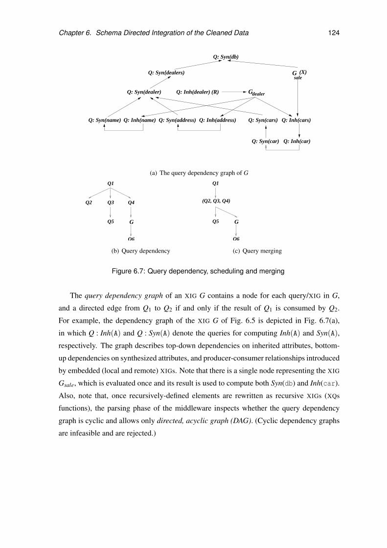
Chapter 6. Schema Directed Integration of the Cleaned Data 124
Gdealer
Q: Inh(car)
Q: Syn(dealer)
Q: Syn(address) Q: Inh(address)
Q: Syn(car)
Q: Syn(db)
Q: Syn{dealers)
Q: Syn(name)
Q: Inh(dealer) (R)
Q: Syn(cars)Q: Inh(name) Q: Inh(cars)
Gsale
(X)
(a) The query dependency graph of G
Q1
Q2 Q3 Q4
Q5
Q6
G
(b) Query dependency
Q1
Q5
Q6
(Q2, Q3, Q4)
G
(c) Query merging
Figure 6.7: Query dependency, scheduling and merging
The query dependency graph of an XIG G contains a node for each query/XIG in G,
and a directed edge from Q1 to Q2 if and only if the result of Q1 is consumed by Q2.
For example, the dependency graph of the XIG G of Fig. 6.5 is depicted in Fig. 6.7(a),
in which Q : Inh(A) and Q : Syn(A) denote the queries for computing Inh(A) and Syn(A),
respectively. The graph describes top-down dependencies on inherited attributes, bottom-
up dependencies on synthesized attributes, and producer-consumer relationships introduced
by embedded (local and remote) XIGs. Note that there is a single node representing the XIG
Gsale, which is evaluated once and its result is used to compute both Syn(db) and Inh(car).
Also, note that, once recursively-defined elements are rewritten as recursive XIGs (XQs
functions), the parsing phase of the middleware inspects whether the query dependency
graph is cyclic and allows only directed, acyclic graph (DAG). (Cyclic dependency graphs
are infeasible and are rejected.)

Chapter 6. Schema Directed Integration of the Cleaned Data 125
Query Scheduling. Based on the query dependencies in an XIG, the XIG-middleware
optimizer orders the execution of queries/XIGs such that local queries and remote XIGs
can be evaluated in parallel. For example, consider the dependency of Fig. 6.7(b), where
Q1, . . . ,Q6 are local queries and G is a remote XIG call. One may want to execute Q4
before Q2 and Q3 such that G can be evaluated by another server in parallel with Q2,Q3,
and thus improve the overall response time. It is, however, nontrivial to develop an optimal
scheduling strategy. Among other things, XIGs are complex tasks and a remote XIG may
trigger other remote XIGs. For example, referring to Fig. 6.6(b), server 1 triggers remote
XIGs at servers 2 and 4, while the remote XIG at server 2 may invoke another XIG at server
4, competing for the resources of server 4.
Query Merging. Another optimization technique is to merge multiple XQs queries into
a single query. For example, an XIG without remote XIG calls can be easily rewritten
as a single XQs query. The merged XQs queries can then be optimized via an XQs opti-
mizer (Fig. 6.6(a)). Query merging could reduce the communication overhead between the
middleware and the underlying XQuery engine, and thus potentially speed up the query ex-
ecution. On the other hand, injudicious query merging may change the query dependency
graph, lead to unnecessary delay of other query executions, and decrease parallelism. For
example, merging Q2,Q3,Q4 of Fig. 6.7(b), results in the query dependency DAG shown
in Fig. 6.7(c). As a result, the remote XIG call G is delayed as it becomes dependent on
Q2 and Q3 as well, thus decreasing the potential parallelism among remote XIGs and local
queries. Clearly, the decision of whether or not to merge certain queries should be cost-
based; furthermore, given the dependence of execution cost on scheduling, query merging
and scheduling are obviously dependent on each other.
Thus one should decide whether or not to merge certain queries based on the costs. In
addition, because of the interaction between query merging and scheduling, the two have
to be dealt with together.
6.4 XIG Evaluation and Optimization
In this section, two cost-based algorithms are presented for scheduling and merging
XQs/XIG expressions to improve the response time of XIG evaluation. These can be com-

Chapter 6. Schema Directed Integration of the Cleaned Data 126
bined with optimizations for XQs queries, i.e. the middleware is open to and can accommo-
date optimization techniques for specific XQuery fragments.
Scheduling an XIG Evaluation. Assume a given query dependency DAG that captures
the data and execution dependencies between the various components (namely, XQs and
XIG expressions) comprising an XIG. Note here that, although XQs queries are typically
executed locally, XIG nodes can be either local or remote (i.e. with the XIG executed at a re-
mote server). Effectively scheduling such an XIG-dependency DAG over an architecture of
distributed servers is a very challenging problem. In addition to all the complications typ-
ically associated with scheduling a DAG of inter-dependent (i.e.precedence-constrained)
tasks over a distributed architecture (e.g. communication overhead, parallel execution), a
crucial, distinguishing characteristic of the problem is that XIGs are complex tasks that can
invoke other (local or remote) XIG tasks for their evaluation. In essence, this means that,
instead of simply utilizing a single server, the evaluation of an XIG node in the query de-
pendency DAG can utilize several different servers (through embedded remote XIG calls).
This strict co-scheduling requirement makes the XIG-scheduling problem quite different
from those studied in the context of conventional scheduling for parallel/distributed sys-
tems, where the assumption is that either each task uses a single site [HM95] or that tasks
can be migrated across different subsets of sites [BFV96, GI97].2 Similarly, work on dy-
namic/adaptive scheduling strategies for distributed database and data-integration systems
(e.g. [IFF+99, BFMV00]) is applicable only at run-time, that is, when the query plan is
actually executed. In contrast, the focus here is on compile-time scheduling in order to
determine an effective XIG-evaluation plan; thus, the scheduling model needs to be able to
capture all the complexities of XIG evaluation.
Given an XIG query dependency graph G, determining a schedule for G over the un-
derlying architecture of distributed servers that minimizes the overall XIG execution time
(i.e. the makespan of the schedule) is an essential step in optimizing XIG evaluation. The
scheduler needs to make its decisions at XIG-optimization time, which means that it needs
to rely on estimates for query/XIG execution costs, result sizes, and communication over-
heads. In the implementation, we assume that each server s in the underlying system offers
2Note that the corresponding scheduling problem for AIG evaluation [BCF+03] also assumesonly single-site queries.

Chapter 6. Schema Directed Integration of the Cleaned Data 127
a query/XIG-costing API that, given a query/XIG node t to be executed at s returns (1) an
estimate l(t) for the processing time of t’s execution on s; and, (2) a subset of sites S(t)
(including s) that are utilized in the evaluation of t (where |S(t)| > 1, if t is an XIG node
with embedded remote XIG calls).3 Thus, for each node t in the dependency graph, the
underlying server APIs provide us with the execution time of t as well as the (sub)set of
servers used during this execution. The XIG-scheduling problem can then be abstracted as
follows.
XIG SCHEDULING( G, S , l(), S() )
• Given: A dependency DAG G = (V,E) defining a partial order (precedence) relation “≺” over a
set of tasks V = {t1, . . . , tn}; set of distributed servers S . For each task t ∈ V , l(t) is the execution
time of t and S(t) ⊆ S is the set of servers used during t’s execution.
• Find: An assignment of start times to tasks start : V → R+, such that:
1. Concurrently-executing tasks do not collide on servers – that is, for all i 6= j, if [start(ti),
start(ti)+ l(ti))] ∩ [start(t j), start(t j)+ l(t j))] 6= φ then S(ti) ∩ S(t j) = φ.
2. Precedence constraints are satisfied – that is, for all ti ≺ t j we have start(t j)≥ start(ti)+ l(ti);
and,
3. The schedule makespan maxi{start(ti)+ l(ti)} is minimized.
It is easy to verify that the XIG-scheduling problem is actually the precedence-
constrained generalization of the Set Scheduling problem recently introduced by Goel
et al. [GHPT99]. Even for their simpler case of fully-independent tasks (i.e. ≺= φ),
Goel et al. demonstrate that the problem is NP-hard and hard to approximate, by giving
a simple, approximation-preserving reduction from the Minimum Graph Coloring prob-
lem [GHPT99]. Given the intractability of the XIG SCHEDULING problem, now a heuristic
scheduling algorithm is proposed for query dependency graphs that produces an approxi-
mate solution to the scheduling problem.
3To simplify the exposition, we assume that the query/XIG-processing time l(t) also includes thecost of communicating input/output data to/from the executing server s, which also allows us toleave result-size estimates out of the scheduling-problem formulation. Both aspects can be incorpo-rated into the scheduling model and algorithms in a straightforward fashion.
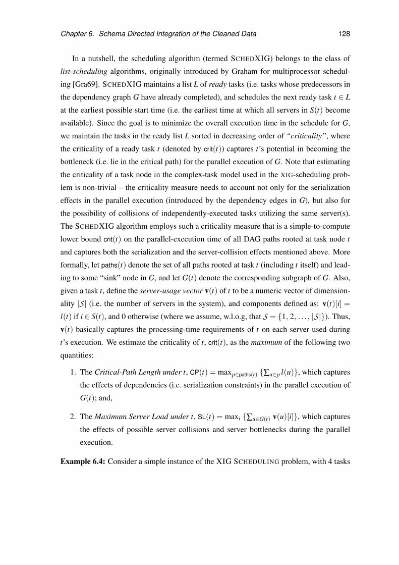
Chapter 6. Schema Directed Integration of the Cleaned Data 128
In a nutshell, the scheduling algorithm (termed SCHEDXIG) belongs to the class of
list-scheduling algorithms, originally introduced by Graham for multiprocessor schedul-
ing [Gra69]. SCHEDXIG maintains a list L of ready tasks (i.e. tasks whose predecessors in
the dependency graph G have already completed), and schedules the next ready task t ∈ L
at the earliest possible start time (i.e. the earliest time at which all servers in S(t) become
available). Since the goal is to minimize the overall execution time in the schedule for G,
we maintain the tasks in the ready list L sorted in decreasing order of “criticality”, where
the criticality of a ready task t (denoted by crit(t)) captures t’s potential in becoming the
bottleneck (i.e. lie in the critical path) for the parallel execution of G. Note that estimating
the criticality of a task node in the complex-task model used in the XIG-scheduling prob-
lem is non-trivial – the criticality measure needs to account not only for the serialization
effects in the parallel execution (introduced by the dependency edges in G), but also for
the possibility of collisions of independently-executed tasks utilizing the same server(s).
The SCHEDXIG algorithm employs such a criticality measure that is a simple-to-compute
lower bound crit(t) on the parallel-execution time of all DAG paths rooted at task node t
and captures both the serialization and the server-collision effects mentioned above. More
formally, let paths(t) denote the set of all paths rooted at task t (including t itself) and lead-
ing to some “sink” node in G, and let G(t) denote the corresponding subgraph of G. Also,
given a task t, define the server-usage vector v(t) of t to be a numeric vector of dimension-
ality |S | (i.e. the number of servers in the system), and components defined as: v(t)[i] =
l(t) if i ∈ S(t), and 0 otherwise (where we assume, w.l.o.g, that S = {1, 2, . . . , |S |}). Thus,
v(t) basically captures the processing-time requirements of t on each server used during
t’s execution. We estimate the criticality of t, crit(t), as the maximum of the following two
quantities:
1. The Critical-Path Length under t, CP(t) = maxp∈paths(t) {∑u∈p l(u)}, which captures
the effects of dependencies (i.e. serialization constraints) in the parallel execution of
G(t); and,
2. The Maximum Server Load under t, SL(t) = maxi {∑u∈G(t) v(u)[i]}, which captures
the effects of possible server collisions and server bottlenecks during the parallel
execution.
Example 6.4: Consider a simple instance of the XIG SCHEDULING problem, with 4 tasks

Chapter 6. Schema Directed Integration of the Cleaned Data 129
V = {t1, . . . , t4} and the task dependencies t1 → t2 → t3, t1 → t4. Assume a 3-server
configuration, and let v(t1) = [2,0,0], v(t2) = [0,8,0], v(t3) = [5,0,0], and v(t4) = [0,0,10].
It is easy to see that, in this scenario, CP(t1) = max{2+8+5, 2+10}= 15 and SL(t1) =
max{[2 + 5, 8, 10]} = 10, which implies that crit(t) = max{CP(t1), SL(t1)} = 15; that
is, the dominant factor in this parallel execution comes from the serialization in the t1→t2→ t3 dependency chain. In contrast, assume that t4 is a complex (XIG) task that utilizes
both servers 2 and 3, i.e. v(t4) = [0,10,10]. It is again easy to see that, in this case, even
though the critical-path length CP(t1) remains the same, the maximum server load becomes
SL(t1) = max{[2 + 5, 10 + 8, 10]} = 18, which implies that crit(t) = SL(t1) = 18 – thus,
the dominant execution-time factor has shifted to the processing bottleneck created by the
collision of t2 and t4 on server 2. 2
The pseudo-code for the SCHEDXIG algorithm is given in Fig. 6.8; its worst-case time
complexity is O(n|S | logn) (e.g. using a max-heap for L). Note that, even though we pre-
sented the algorithm SCHEDXIG as an optimization-time technique, it is actually an on-
line algorithm that can readily be used to schedule XIG executions at run-time (based on
task-criticality estimates) as servers become available. Finally, we should note that the
complex-task model can be generalized along the lines of the preemptable/time-shared re-
source model of [GI97] to allow for servers to be effectively time-shared across different
tasks, since, e.g. an XIG node can typically impose different processing requirements on
the remote servers it utilizes. This gives rise to several challenging scheduling issues that
we are exploring in the ongoing work.
Merging Queries. Query merging may also speed up XIG evaluation; however, it can
also change the dependency DAG and, thus, the execution schedule (and corresponding
evaluation cost). Thus, query merging and scheduling are clearly inter-dependent. The
query merging problem is to determine, given a dependency graph G, what query nodes to
merge such that the estimated response time of the resulting dependency graph G′ (i.e. the
makespan of the schedule returned by SCHEDXIG (G′)) is minimized.
Given a dependency graph G, there are exponentially many choices for merging queries
in G; moreover, recall that the scheduling problem is already intractable. Given the inher-
ent difficulty of the problem, we outline a greedy heuristic algorithm, termed MERGEXIG,
that iteratively calls the SCHEDXIG scheduler for optimizing XIG query merging and eval-

Chapter 6. Schema Directed Integration of the Cleaned Data 130
Procedure SCHEDXIG (G,S)
Input: XIG dependency graph G, set of servers S .
Output: Schedule start() for executing G over S .
begin
1. for each node t in G do
2. compute crit(t) := max{CP(t),SL(t)}3. L := list of ready XQs/XIG tasks in G in decreasing order of crit(t)
4. while L 6= φ do
5. t := L[1] /* first ready task in L*/
6. start(t) := earliest time in the schedule that all servers in S(t)
become available
7. M := list of tasks in G that become ready after the
completion of t (in decreasing crit())
8. L := merge(L−L[1],M)
9. endwhile
endFigure 6.8: The XIG-Scheduling Algorithm.
uation. In a nutshell, MERGEXIG takes an XIG dependency graph G as input and returns
an efficient evaluation schedule as output. At each step, MERGEXIG considers each pair of
query nodes (Q1,Q2) in G that are processed at the same source for potential merging into
a single query node Q (resulting in a new dependency graph G′); the query pair resulting in
the (acyclic) dependency graph G′ with the lowest SCHEDXIG-estimated evaluation cost
(i.e. the smallest makespan for SCHEDXIG (G′)) is merged. The iteration in MERGEXIG
continues until no further cost reduction is possible; at that time, SCHEDXIG is invoked
on the final (merged) dependency graph to determine the final XIG execution schedule.
It is easy to see that the worst-case time complexity of MERGEXIG (or, the entire XIG
optimization procedure) is O(n3|S | logn).
Next, we consider how to merge a pair of queries, namely, given a query pair (Q1,Q2),
how to generate a single query Q to compute both Q1 and Q2. For a pair of queries that are
not dependent on each other, the merged query can be simply expressed as:

Chapter 6. Schema Directed Integration of the Cleaned Data 131
<result> <q1>{Q1}</q1> <q2>{Q2}</q2> </result>
It is straightforward to separate and extract the results of Q1 and Q2 from the result of the
merged query.
Now, consider a pair (Q1,Q2) where Q2 uses the result of Q1. In particular, consider a
production A→ α, and we want to merge the queries for computing Inh(A) (Q1) and Inh(B)
(Q2), where B is in α. If Q1 yields a sequence of values of Inh(A), we want the merged
query Q to compute a corresponding sequence of Inh(B) values. We associate a “key”
with each value of Inh(B) in order to determine the position of the B element in the target
XML document. The key of an Inh(B) value is generated by concatenating the key of the
corresponding Inh(A) value $x and an id fsk($x). Here fsk is a Skolem function that, given a
value, generates a unique id (see, e.g. [Kos96] for discussions on Skolem functions). Using
the keys, the synthesized attribute Syn(A) can be computed by sort-merging the values of
Syn(B) for all B in α w.r.t. key values.
For example, recall the rules associated with a production A→ B1, . . . ,Bn (similarly for
other productions). Let query Q1 compute Inh(A) and return either a single s-element
<s> <val> v </val> <key> k </key> </s>,
or a sequence of s-elements enclosed by a tag <seq>, where v is a value of Inh(A) and k is
the key of v. Then, the merged query for computing Inh(Bi) is (abusing XQuery syntax):
let $a := Q1 return
{if $a/s
then <s> <val>{Qi($a/s/val)}</val><key>{($a/s/key, fsk($a/s/val))}</key> </s>
else <seq> for $a’ in $a/seq/s
let $v := $a’/val
let $k := $a’/key
return <s> <val>{Qi($v)}</val><key>{($k, fsk($v))}</key> </s>
</seq>}
The query returns either a single pair (Inh(B), key) or a sequence of such pairs depending
on the input Inh(A). (Note that the sibling and parent/child relations are captured by the
keys.) This example shows how to merge a pair of queries with dependency on them.

Chapter 6. Schema Directed Integration of the Cleaned Data 132
It is worth mentioning that the query-merging strategy given above does not introduce
any null values, in contrast to the out-union/outer-join approaches of [BCF+02, BCF+03,
FMS01, CFI+00].
6.5 Experimental Evaluation
0
100
200
1000 3000 5000 7000 9000
Ela
psed
tim
e (s
ec)
|DB|
w query mergingw/o query merging
Figure 6.9: Effectiveness of query merging on XIG Gdealer
Next, the preliminary results from an experimental evaluation of the XIG-based tech-
niques is presented. A prototype of XIG-based middleware has been built on top of the
Galax XQuery engine (db.bell-labs.com/galax) and Java RMI. The source databases are
built based on the source DTD DSdealer and DS
dealer by using the Toxgene data generator
(www.cs.toronto.edu/tox/toxgene). The database size, |DB|, is given as the number of
cars. A fraction f of the cars are on sale. For the recursive definition of feature in the
sale data (recall DSsale from Fig. 6.1), 1 to 3 random features are generated for each car and
the depth of the recursion is limited to 2. The experiments were run on a distributed sys-
tem connected by a local area Ethernet. Each site has a 2.4GHz Pentium 4 processor and
512M RAM. Unless otherwise stated, each experiment was run 5 times and the average is
reported.
Query Merging. Figure 6.9 shows the impact of query merging on the performance of

Chapter 6. Schema Directed Integration of the Cleaned Data 133
the XIG Gdealer for different database sizes. Since Gdealer only involves a single server,
scheduling is not needed here. The results clearly indicate that the evaluation strategy with
query merging outperforms the one without merging. The performance gain is about 30%
for large databases. Note that the gain comes from reducing the number of Galax calls,
as Galax does not support query optimization and thus merged queries are not optimized
by Galax. The performance gain from query merging is expected to be further improved
pending the availability of optimization in XQuery engines (to our knowledge, no stable
XQuery engine supports all of our queries and optimizations).
Our Alg.optimal
6 8 10 12 14 16 18 20R
6 8 10 12 14 16 18 20N
1000 2000 3000 4000 5000 6000
Elapsed time (sec)
Figure 6.10: Scalability and benefits of query composability
Query Composability. The next set of experiments verifies the scalability and benefits of
our XIG evaluation algorithm (namely, SCHEDXIG and MERGEXIG put together) with two
workloads W1 and W2. To better demonstrate the impact of remote XIG calls, W1 slightly
extends the XIG G(R,X) of Fig. 6.5 by adding a remote XIG which encodes the join in the
rule for computing Inh(car), while W2 further extends Gdealer in W1 by adding an extra
join on the car model. Both workloads were run on the distributed system. Figure 6.10
compares the evaluation time of W2 obtained by using the evaluation algorithm with that
of an optimal scheduling and merging strategy, which is computed manually as the XIGs
involved are simple. In Fig. 6.10, |DB| and f are fixed as 5000 and 10%, respectively. The
number of servers N and the number of URIs R are varied from 5 to 20. The remote calls are
uniformly distributed over the servers. The results show that our algorithm performs well;
indeed, its performance nearly matches the optimal one. Furthermore, Fig. 6.10 indicates

Chapter 6. Schema Directed Integration of the Cleaned Data 134
that our algorithm also scales well – its evaluation time decreases when the number N of
servers increases, i.e. it is roughly linear in 1/N; moreover, the performance is better when
the N/R ratio gets larger. The results of evaluating W1 are similar.
0
100
200
300
400
500
600
700
800
2 4 6 8 10 12 14 16 18 20
Ela
psed
tim
e (s
ec)
N
CRITLTFSTF
Figure 6.11: Effectiveness of XIG-Scheduling
Scheduling. To study workload sensitivity of our criticality-based XIG-Scheduling al-
gorithm (denoted as CRIT), we compare its performance with two traditional schedul-
ing algorithms Shortest Task First (STF) and Longest Task First (LTF) using randomly-
generated XIG query-dependency graphs. Table 6.1 gives parameter settings for our ran-
dom dependency-graph generator. Each node in a graph has a single parent (i.e. fan-in of
1), whereas node fan-out is chosen uniformly between 2 and 4. The length of root-to-leaf
path is chosen uniformly between 4 and 8. The probability of a node being an XIG call is
0.5, and its execution site is distributed uniformly among all servers. The ranges of costs
for queries and XIG-calls are determined based on the response times obtained by using our
prototype. Figure 6.11 depicts the performance of the algorithms. Each simulation was run
100 times to obtain sufficient confidence intervals of average elapsed times. The number
of servers, N, varies from 2 to 15. Clearly, when N is small (e.g. N = 2), scheduling is a
non-issue and all algorithms perform similarly. However, as N increases, CRIT does better
at exploiting parallelism, and it outperforms STF and LTF by more than 40% and 60%,
respectively.
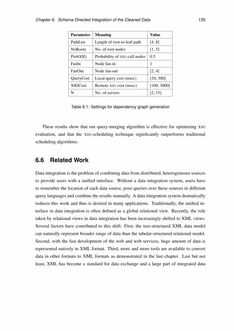
Chapter 6. Schema Directed Integration of the Cleaned Data 135
Parameter Meaning Value
PathLen Length of root-to-leaf path [4, 8]
NoRoots No. of root nodes [1, 5]
ProbXIG Probability of XIG-call nodes 0.5
FanIn Node fan-in 1
FanOut Node fan-out [2, 4]
QueryCost Local query cost (msec) [10, 300]
XIGCost Remote XIG cost (msec) [100, 3000]
N No. of servers [2, 15]
Table 6.1: Settings for dependency graph generation
These results show that our query-merging algorithm is effective for optimizing XIG
evaluation, and that the XIG-scheduling technique significantly outperforms traditional
scheduling algorithms.
6.6 Related Work
Data integration is the problem of combining data from distributed, heterogeneous sources
to provide users with a unified interface. Without a data integration system, users have
to remember the location of each data source, pose queries over these sources in different
query languages and combine the results manually. A data integration system dramatically
reduces this work and thus is desired in many applications. Traditionally, the unified in-
terface in data integration is often defined as a global relational view. Recently, the role
taken by relational views in data integration has been increasingly shifted to XML views.
Several factors have contributed to this shift: First, the tree-structured XML data model
can naturally represent broader range of data than the tabular-structured relational model.
Second, with the fast development of the web and web services, huge amount of data is
represented natively in XML format. Third, more and more tools are available to convert
data in other formats to XML formats as demonstrated in the last chapter. Last but not
least, XML has become a standard for data exchange and a large part of integrated data

Chapter 6. Schema Directed Integration of the Cleaned Data 136
often needs to be exchanged. Thus, XML data integration is highly demanded in modern
information systems.
Although a number of integration systems have been developed for semistructured data
and XML [BGL+00, BGK+02, CDSS98, GMPQ+97, CFI+00, FMS01, MZ98, PVM+02],
they typically provide very little support for modularity or ensuring DTD-conformance, es-
pecially when the prescribed DTD is recursive and/or non-deterministic. Clio [PVM+02]
derives schema and data mappings from constraints; it is unclear how it can ensure DTD
conformance automatically. MIX [BGL+00] considers DTD checking/inference for XML
integration, but the inference process is expensive, and does not provide any guidance
for how to define a mapping that type-checks [PV00]. XML publishing systems such
as SilkRoute [FMS01], XPERANTO [CFI+00, SSB+01b] and ROLEX [BGK+02] con-
sider only a single relational source and do not take DTDs into account. Earlier sys-
tems [CDSS98, GMPQ+97, MZ98] are either developed for semistructured data without
a type system, or based on schema-matching; it is unclear how they can automatically
guarantee DTD-conformance when the source and target schemas involved are dramati-
cally different, or if the integration depends on the application rather than merely upon the
schemas. Furthermore, none of these systems addresses modularity for integration specifi-
cations. Similarly, in the realm of commercially-available systems, support for modular,
DTD-directed XML data integration is either non-existent or still at a fairly primitive stage.
Nimble’s Integration suite (www.nimble.com) allows users to pose queries over distributed
XML data sources to synthesize a result XML document but does not address the issues of
schema conformance or modular integration specifications. BEA’s WebLogic Integration
and Liquid Data suites (www.bea.com) allow for XML-to-XML transformations through a vi-
sual mapping tool that allows users to specify simple matchings between schema elements;
it is unclear how these tools can be used to specify complex, hierarchical integration with
a complicated target DTD.
Active XML (AXML) [ABC+03a, MAA+03] proposes a novel notion of intentional XML
documents with embedded function calls to remote Web services. AXML is designed to sup-
port data exchange and Web-service calls via an unlimited class of embedded functions;
furthermore, it also supports XML data integration through the use of XML tree templates
with embedded function calls. However, this template-based approach to integration can
typically only produce mild variations of a fixed document structure. The functionality of

Chapter 6. Schema Directed Integration of the Cleaned Data 137
AXML for supporting embedded Web services is, in a sense, complementary to the prob-
lem of DTD-directed XML integration, where the goal is to construct an integrated view
guaranteed to conform to a predefined, possibly complex DTD.
It is worth mentioning that XIGs are not targeted for providing the functionalities of
AXML to support Web services; they are complementary to AXML by providing guarantee
for generating XML documents that conform to predefined DTDs when it comes to XML
integration, instead of producing mild variations of a fixed document.
Closest to this work are Attribute Integration Grammars (AIGs), a grammar-based for-
malism for schema-directed integration of relational data in XML [BCF+02, BCF+03].
AIGs extend a target DTD with tuple-valued attributes and SQL queries over the relations.
These earlier proposals are, however, inadequate for XML integration. First, they are re-
stricted to flat, relational sources [BCF+02, BCF+03]. Second, and perhaps most im-
portantly, while AIGs guarantee schema-conformance, they are not composable: a large
integration task must be specified with a single AIG on top of a large DTD. Developing
an effective, modular solution for large-scale, DTD-directed XML data integration poses a
whole new set of difficult research challenges, including the need for a significantly more
powerful, composable formalism and novel optimization/evaluation techniques.

Chapter 7
Selective Exposure of the Integrated
Data
In many applications users are allowed to access an XML document only by querying a
view of the data. The need for this is evident in, for example, enforcing access control on
XML data [CAYLS02, DdVPS00, FCG04]. To prevent improper disclosure of sensitive or
confidential information of XML data residing in a server, the administrator defines an XML
view for each group of users, consisting of all and only the information that the users are
authorized to access. While the users may query the view, they are not allowed to directly
query or access the underlying document (referred to as the source). With this comes the
need to answer queries posed on the views. One way to do this is to first materialize the
views and then directly evaluate queries on the views. However, it is often too costly to
materialize and maintain a large number of views, a common scenario when many groups
of users with different access privileges query the same source. A more realistic approach
is to rewrite (aka. translate, reformulate) queries on the views into equivalent queries on
the source, evaluate the rewritten queries on the source without materializing the views,
and return the answers to the users.
This chapter studies how to rewrite XML queries posed on virtual XML views into equiv-
alent queries on the underlying XML document. For XML queries we start with a fragment
of XPath, which supports recursion (the descendant-or-self axis ‘//’), union and complex
filters (predicates). This class of XPath queries is commonly used in practice and is essen-
tial to XQuery, XSLT and XML Schema. We consider XML views defined by annotating a
138

Chapter 7. Selective Exposure of the Integrated Data 139
view DTD with a collection of (regular) XPath expressions, along the same lines as how
commercial systems specify XML views [IBM, Ora, Mic05]. An XML view defined as
above is a mapping σ : D→ DV in the global-as-view style, from XML documents of the
document DTD D to documents of the view DTD DV . When the view schema DV is recur-
sively defined, i.e. if some element type in DV is defined in terms of itself, so is the view.
The central technical problem studied in this chapter is:
The rewriting problem is to find an algorithm that, given a view definition σ and an
XPath query Q over the view DTD DV , computes an XPath query Q′ over the document
DTD D such that for any XML tree T of D, Q(σ(T )) = Q′(T ).
While there has been a host of work on rewriting XPath queries into SQL queries for
XML views of relational data (see [KCKN04] for a survey), little previous work has con-
sidered rewriting XPath queries into XPath queries for XML views which can hide arbitrary
nodes of XML data. In this context, query rewriting has only been studied for non-recursive
XML views, over which XPath rewriting is always possible [FCG04]. However, query
rewriting for recursive views is still an open problem [KCKN04].
Recursive DTDs naturally arise when, e.g., specifying biomedical data (see the Gene
Ontology database, GO [EBI]); in fact [Cho02] shows that out of 60 real-world DTDs an-
alyzed, more than half (35) of them were recursive. It is the reason that Oracle supports
fully recursively defined XML views (AXSD [Ora]) and that IBM also allows a class of re-
cursively defined XML view (DAD [IBM]). However desirable, the rewriting problem is
more intriguing for recursively defined views, due to the interaction between recursion in
XPath queries (e.g., ‘//’) and recursion in the view definition.
Example 7.1: Consider a hospital DTD D shown as a graph in Fig. 7.1. A hospital doc-
ument of D consists of a list of departments, and each department has a list of in-patients
(i.e. patients who are currently residing in the hospital; we use ‘∗’ on an edge to indicate a
list). For each patient, the hospital maintains her name (pname), address, records of visits,
each including the visit date and treatment which is either a test or some medication (dashed
edges indicate disjunction), as well as information about the treating doctor. Each name,
pname, street, city, zip, date, type, dname, specialty has a single text node (PCDATA) as its
child (omitted in the figure). The hospital also maintains family medical history by means
of the recursively defined parent and sibling. It records the same information of ancestors

Chapter 7. Selective Exposure of the Integrated Data 140
Figure 7.1: Example: document DTD D.
(a) view DTD DV
production: hospital→ patient∗
σ0(hospital,patient) = department/patient[visit/treatment/
medication/diagnosis/text() = ‘heart disease’] /*Q1*/
production: patient→ parent∗, record∗
σ0(patient, parent) = parent /*Q2*/
σ0(patient, record) = visit /*Q3*/
production: parent→ patient
σ0(parent, patient) = patient /*Q4*/
production: record→ empty + diagnosis
σ0(record, empty) = treatment/test /*Q5*/
σ0(record, diagnosis)= treatment/medication/diagnosis /*Q6*/
(b) view specification
Figure 7.2: Example: view DTD and view specification.
with those of in-patients, by sharing the description for patients.
A view σ0 is defined for a research institute studying inherited patterns of heart disease,
with the view DTD depicted in Fig. 7.2 (the view is defined in Example 7.3). Obliged by
the Patient Privacy Act, the view reveals only those patients who have heart disease, along

Chapter 7. Selective Exposure of the Integrated Data 141
with their parent hierarchy. While the institute may access diagnosis information of those
patients and their ancestors, it is denied access to their name, address, test and doctor data.
Consider an XPath query Q posed on the view, which is to find patients whose ancestors
also had heart disease:
Q: patient[*//record/diagnosis/text()=‘heart disease’].
Here ∗ denotes a wildcard, i.e., any element. However, it is impossible to rewrite Q on the
view to an equivalent query (in the XPath fragment mentioned above) on the underlying
hospital document. This is because ‘//’ in Q is supposed to traverse only the parent hierar-
chy on the view, i.e., a sequence of the (parent/patient) pattern; however, when translated
to a query Q′ on the source, Q′ necessarily retains ‘//’ since the view DTD is recursive, and
‘//’ in Q′ may access siblings of those patients, although siblings are not in the view and are
not allowed to be accessed. An incorrect translation may lead to serious security breach.
2
In response to this both fundamental results and practical techniques for the rewriting
problem have been developed in this chapter.
7.1 XML Security Sub-framework
Views are commonly used in traditional (relational) databases to enforce access control,
and therefore provide a promising method to access XML data securely. In CLINSE, an
XML security sub-framework has been designed to protect the integrated XML data. The
sub-framework is based on the novel concept of security views proposed in [FCG04], which
provide for each user group a virtual XML view consisting of all and only the information
that the users are authorized to access, and a view DTD that the XML view conforms to.
As depicted in Fig. 7.3, the sub-framework consists of three primary modules (view
derivation and query rewriting, evaluation) and four secondary modules (access policy
editor, security view editor, query editor, and result viewer). Briefly, the secondary mod-
ules implement a user-friendly interface through which the user interacts with the sys-
tem. The primary modules implement all the basic algorithms and functionality of the
sub-framework. They are internal and thus users do not directly interact with them.
Central to the sub-framework is a number of security views which tailor the XML docu-

Chapter 7. Selective Exposure of the Integrated Data 142
ResearchersInsurersDoctors
XMLdocument T
View Derivation
Query Rewriting
Query Evaluation
...
legend
QueryEditor
Access PolicyEditor
ResultViewer
security administrators researchers
user group
XML schema
DTD Dfor
document T
XML data flow
other data flow
XML doc/view
Security ViewEditor
DTD DD DTD D
I DTD DR
SecurityView V
D
SecurityView V
I
SecurityView V
R
Access Policy PQuery Q
R on V
R
Query QT
on T
Figure 7.3: The XML security sub-framework
ment for different user groups by hiding the un-authorized information. Two types of users
interact with the sub-framework, namely, security administrators who specify the access
policies or security views for each user group, and users in a certain group who query the
XML views to which they have been granted access.
To illustrate the sub-framework, suppose that several user groups, such as researchers,
insurers and doctors, need to access the medical records in Fig. 7.1. As shown in Fig. 7.3, it
works as follows. First, using the access policy editor, the security administrators specify
the access policies P for each group as annotations in the DTD of the XML documents.
The policies P are then passed to the view derivation module where a set of security view
definitions VR, VI , VD and their DTDs DR, DI , DD are automatically derived from P for the
groups of researchers, insurers, and doctors, respectively. Next, users in each group are
allowed to pose queries over the virtual security view using the query editor. This process
is assisted by providing users with a corresponding view DTD. For instance, a user UR in
the group of researchers poses a query QR over view VR. In the query rewriting module,
this query QR is subsequently rewritten into a new query QT over the underlying document
T . Query QT is passed to the query evaluation module to be executed over the document
T . Finally, the result of QT (and therefore QR) is shown in the result viewer to the user
UR. In the environments requiring more flexibilities, the views VR, VI and VD could also

Chapter 7. Selective Exposure of the Integrated Data 143
be manually defined by the security administrators with the assistance of the security view
editor.
In the worst case, four languages are involved in the sub-framework: the access specifi-
cation language LA and the view specification language LV are used by the security admin-
istrators to specify access policies and security views, respectively; the view query language
LVQ and the document query language LT
Q are used by the users to pose queries over the XML
data. LV and LTQ are also used by the view derivation and query rewriting modules, respec-
tively, for representing the automatically generated view definitions and queries. Solutions
for the view derivation have been provided in [FCG04]. Moreover, in the settings where
the security views are manually specified, view derivation module is not needed. In the
remainder of this chapter, the query rewriting and evaluation problems, which are not fully
solved in [FCG04], are investigated and the requirements of languages LV , LVQ and LT
Q are
studied.
7.2 XML Queries and View Specifications
In this section we review the candidates of view specification language LV , view query
language LVQ and document query language LT
Q considered in this chapter.
7.2.1 XPath and Regular XPath
In this chapter, the downward fragments of XPath and regular XPath, i.e., X ↓,∗;∗∪;[¬,=] and
X ↓;∗∪,∗;[¬,=] defined in Section 5.3, are considered. Hereafter they will be simply written as
X and XR, and the simplified syntax is adopted. For example, regular XPath [Mar04b] XR
is simplified as:
Q ::= ε | A | ↓ | Q/Q | Q∪Q | Q∗ | Q[q],
q ::= Q | Q/text() = ‘c’ | ¬Q | Q∧Q | Q∨Q
where ε is the empty path (self), A is a label (tag), ↓ is a wildcard (i.e., the ∗ inside of a
node test in the un-simplified syntax), ‘∪’ represents union, ‘/’ is the child-axis, and ∗ is
the Kleene star; [q] is referred to as a filter, in which Q is an XR expressions, c is a string
constant, and ¬,∧,∨ are the Boolean negation, conjunction and disjunction, respectively.

Chapter 7. Selective Exposure of the Integrated Data 144
Note that, instead of the ∗ used in Section 5.3, ↓ is used to denote a wildcard to avoid the
confusion with a Kleene star.
Like XPath queries, when an XR query Q is evaluated at a node v in an XML tree T , it
returns the set of nodes of T reachable via Q from v, denoted by v[[Q]].
Similarly, the simplified syntax of downward XPath X is defined by replacing Q∗ with
‘//’ in the definition above.
Example 7.2: Consider an XML document T conforming to the document DTD D in
Fig. 7.1. The regular XPath query
Q = department/patient[ q0 ∧ (q1/(q1)∗)]/pname
q0 = visit/treatment/medication/diagnosis/text() = “heart disease”
q1 = parent/patient[¬q0]/parent/patient[q0]
when evaluated on T , returns the names of patients who have heart disease and the disease
appears in their ancestors but always skips a generation. Such queries, which look for
certain patterns, are often encountered in medical research. Note that the query is in the
fragment XR, but is not expressible in the XPath fragment X . 2
Regular XPath extends regular expressions by allowing filters [Mar04b, Koz97], and
extends XPath by supporting general Kleene closure Q∗ as opposed to restricted recursion
‘//’. The tradeoff of the expressive power is the additional complexity for query evaluation:
(a) recursion can no longer be captured by a simple ancestor-descendant labeling as for its
XPath counterpart [LM01, KMS02, SHYY05]; and (b) worse still, recursion in an XR query
may be nested: the sub-query Q of Q∗ may itself contain Kleene closure, which we do not
encounter when evaluating XPath queries.
This chapter focuses on regular XPath queries with only downward modalities since
they are most commonly used in practice. As will be seen shortly, rewriting queries is
already challenging in this setting. It is thus necessary to understand rewriting of these
basic queries before dealing with full-fledged XPath or XQuery.
7.2.2 XML Views
We consider views defined by annotating a DTD [FCG04]. This is similar in spirit to
XML view specification in commercial systems, e.g. annotated XSD’s (AXSD) in Oracle

Chapter 7. Selective Exposure of the Integrated Data 145
XML DB [Ora] and Microsoft SQL Server 2000 SQLXML [Mic05], and Document Access
Definitions (DAD) of IBM DB2 XML Extender [IBM].
Specifically, an XML view is a mapping σ : D→ DV , where D is a document DTD, DV
is a view DTD. Given an XML document T of D, the mapping generates an XML view σ(T )
that conforms to the view DTD DV . More specifically, for each element type A and its child
type B in DV (i.e., each edge (A,B) in the DTD graph of DV ), σ maps (A,B) to a query
σ(A,B) defined on documents T of D. Intuitively, given an A element, σ(A,B) generates its
B children in the view by extracting data from T . The query σ(A,B) is in the regular XPath
fragment XR given above. The XML view is recursive if the view DTD DV is recursive.
Example 7.3: The view σ0 described in Example 7.1 can be defined based on the view
DTD DV of Fig. 7.2(a), as shown in Fig. 7.2(b). 2
To give the semantics of σ, we present a materialization strategy that, given an XML
tree T of the document DTD D, computes the view σ(T ), as follows. A partial tree TV is
initialized by copying the root of T and treating it as the root of TV , and this node is marked
unexpanded. The tree TV is then grown by repeatedly selecting an unexpanded b (of some
element type A), evaluating the query σ(A,B) for each child type B of A to generate the
children of b, and marking b expanded. Specifically, we find the production p = A→ P(A)
in DV , and generate the children of b based on the structure of P(A) as follows.
(1) If P(A) is B1, . . . ,Bn, then for each Bi, the query σ(A,Bi) is evaluated on the document
T at the context node b. If Bi is of the form B∗, then each node returned by the query is
treated as a distinct B child of b in the partial tree TV . If Bi is of the form B and the query
returns a single node, the node is treated as a B child of b in TV . Otherwise the computation
aborts for violating the production A→ P(A) of the view DTD. In both cases, if the view
DTD enforces a different label to the nodes returned by the mapping query, these nodes
will be re-labeled to Bi in the view.
(2) If P(A) is B1 + · · ·+ Bn, then for each i ∈ [1,n], the query σ(A,Bi) is evaluated on T
at context node b. If there exists one and only one i ∈ [1,n] such that σ(A,Bi) returns a
nonempty set of nodes without violating the cardinality constraint of Bi as described in (1)
above, then these nodes are treated as the children of b in TV ; otherwise, the computation
aborts. The returned nodes will be re-labeled similarly when there are conflicts between

Chapter 7. Selective Exposure of the Integrated Data 146
the labels in the view and in the document.
(3) If P(A) is str, the query σ(A, str) is evaluated on T at context node b. If it returns a
single text node in T , and the node is treated as the only child of b in TV ; otherwise, the
computation aborts.
(4) If P(A) is ε, nothing needs to be done.
The element children of the node b become new unexpanded and are also processed.
The process proceeds until the partial tree TV cannot be further expanded, i.e., it has no
unexpanded node, or the computation is aborted. The fully expanded TV is the view σ(T ).
Note that σ(T ) is guaranteed to conform to the view DTD DV .
Under this view specification language, there is a many-to-one correspondence between
the nodes in the view and the nodes in the underlying XML document: no new XML node
is constructed in the view; each XML node in the view is mapped from the XML document
through a regular XPath query. We say a node in the view σ and a node in the XML docu-
ment are identical under view σ if they are corresponded to each other in the definition of
σ.
Now we are able to define the query rewriting problem more precisely:The rewriting problem is to find an algorithm that, given a view definition σ and a query
Q over the view DTD DV , computes a query Q′ over the document DTD D such that for
any XML tree T of D, the answer nodes of Q(σ(T )) and those of Q′(T ) are identical
under view σ.
In W3C XPath specification, the answer of a query is node set, number, string or
boolean. In our extended XPath fragment, both the original query on the view and the
rewritten query on the XML document return a node set(number, string or boolean answer
does not apply to this fragment). The two node sets are identical under the view definition.
If the user requires a node set as the answer, this is sufficient. In the cases where the user
also requires the subtrees rooted at each node in the returned node set, more processing are
needed.
The above defined view has a property: a subtree of the view, referred to as subview,
could be evaluated without materializing other parts of the view. To materialize a subview,
a context node in the XML document needs to be mapped as the root of the subview. This
provides the flexibility to materialize arbitrary subviews to save unnecessary computations.
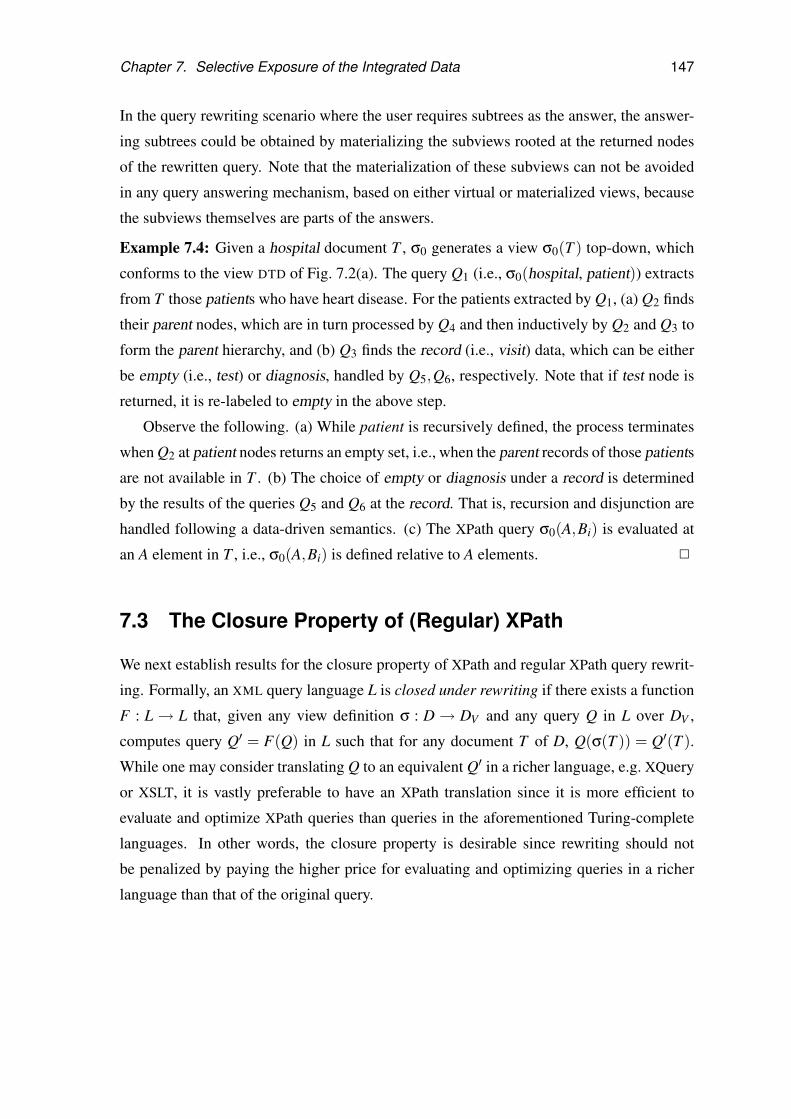
Chapter 7. Selective Exposure of the Integrated Data 147
In the query rewriting scenario where the user requires subtrees as the answer, the answer-
ing subtrees could be obtained by materializing the subviews rooted at the returned nodes
of the rewritten query. Note that the materialization of these subviews can not be avoided
in any query answering mechanism, based on either virtual or materialized views, because
the subviews themselves are parts of the answers.
Example 7.4: Given a hospital document T , σ0 generates a view σ0(T ) top-down, which
conforms to the view DTD of Fig. 7.2(a). The query Q1 (i.e., σ0(hospital, patient)) extracts
from T those patients who have heart disease. For the patients extracted by Q1, (a) Q2 finds
their parent nodes, which are in turn processed by Q4 and then inductively by Q2 and Q3 to
form the parent hierarchy, and (b) Q3 finds the record (i.e., visit) data, which can be either
be empty (i.e., test) or diagnosis, handled by Q5,Q6, respectively. Note that if test node is
returned, it is re-labeled to empty in the above step.
Observe the following. (a) While patient is recursively defined, the process terminates
when Q2 at patient nodes returns an empty set, i.e., when the parent records of those patients
are not available in T . (b) The choice of empty or diagnosis under a record is determined
by the results of the queries Q5 and Q6 at the record. That is, recursion and disjunction are
handled following a data-driven semantics. (c) The XPath query σ0(A,Bi) is evaluated at
an A element in T , i.e., σ0(A,Bi) is defined relative to A elements. 2
7.3 The Closure Property of (Regular) XPath
We next establish results for the closure property of XPath and regular XPath query rewrit-
ing. Formally, an XML query language L is closed under rewriting if there exists a function
F : L→ L that, given any view definition σ : D→ DV and any query Q in L over DV ,
computes query Q′ = F(Q) in L such that for any document T of D, Q(σ(T )) = Q′(T ).
While one may consider translating Q to an equivalent Q′ in a richer language, e.g. XQuery
or XSLT, it is vastly preferable to have an XPath translation since it is more efficient to
evaluate and optimize XPath queries than queries in the aforementioned Turing-complete
languages. In other words, the closure property is desirable since rewriting should not
be penalized by paying the higher price for evaluating and optimizing queries in a richer
language than that of the original query.

Chapter 7. Selective Exposure of the Integrated Data 148
It was shown in [FCG04] that the class X of XPath queries defined in Section 7.2 is
closed under query rewriting for non-recursive views. However, it is shown below that in
the presence of recursion in a view definition, this is no longer the case (even when the
annotating queries are in X ).
Theorem 7.3.1 For recursively defined XML views, the fragment X is not closed under
query rewriting.
Intuitively, the complication is introduced by ‘//’ in X queries posed on a recursive view.
It is impossible to rewrite ’//’ by enumerating the matching label paths in the view DTD,
since it may lead to infinitely many paths due to the recursion in the view DTD. Thus ‘//’
needs to be captured by a recursive operator over the document which is, often necessarily,
the Kleene star operator. A key property of Kleene star, not shared by ‘//’, is that it can
prevent the traversal of data that are in the document but not in the view, which is of central
importance in the security setting, among other things.
Proof:Consider the query Q0 = (↓ / ↓)∗. When it is evaluated at the root of an XML tree T , it
retrieves all nodes in T which are an even number of steps away from the root. It is known
that this query Q0 is not first order definable on trees [Tho84], and thus not expressible in
XPath [Mar04b]. We now construct an XML view σ0 and an XPath query Q1 on the view,
such that any rewritten query Q′1 of Q1 on the source document is equivalent to Q0. Since
query Q0 is not expressible in XPath, the rewritten query Q′1 can not be in XPath, either.
This shows that XPath is not closed under query rewriting.
It remains to construct view σ0 and query Q1. Since we do not want to impose any
restrictions on document T , we set its DTD D to be empty. We define the XML view σ0 :
D→ DV recursively as:
production: r→ A∗
σ0(r,A)= ↓ / ↓
production: A→ A∗
σ0(A,A) = ↓ / ↓.
where A is an arbitrary label. Clearly σ0(T ) extracts all nodes which are an even number
of steps away from the root of T in the same way as query Q0 does. By simply defining

Chapter 7. Selective Exposure of the Integrated Data 149
Q1 = //A, i.e., by retrieving all the nodes in σ0(T ), it is clear that any rewritten query on
the source document should be equivalent to Q0. 2
In contrast, the fragment XR of regular XPath given in the last section is closed under
query rewriting:
Theorem 7.3.2 For arbitrary XML views (recursive or non-recursive), XR is closed under
rewriting.
Proof: This is a direct consequence of the equivalence of MFA and XR queries [FGJK07]
and Theorem 7.5.1. 2
Given that XR subsumes X , an immediate result of Theorem 7.3.2 is that all X and XR
queries on any view can be rewritten to equivalent XR queries on the source. To perform
the rewriting, we can traverse the view DTD graph DV via Q, replacing each encountered
edge (A,B) with σ(A,B). A tricky issue concerns the translation of p∗ (or ‘//’) at a context
node A, denoted by REGx(p∗,A). The rewritten XR query REGx(p∗,A) is to capture all
the label paths from A to nodes reached via p∗. This often requires to construct a NFA to
characterize these paths. This NFA is then converted into a regular expression in order to
obtain the expression for p∗.
Example 7.5: Recall the X query Q given in Example 7.1 and the view σ0 defined in
Example 7.3. While Q cannot be rewritten into Q′ in X on the source T , it can be rewritten
to an equivalent regular XPath query Qr in XR over T (Using the queries Q1,Q2,Q3, Q4 and
Q6 from the view specification in Fig. 7.2(b)):
Qr : Q1[Q2/Q4/(Q2/Q4)∗/Q3/Q6/text()=‘heart disease’],
i.e., department/patient[visit/treatment/medication/diagnosis/
text()=‘heart disease’ ∧ parent/patient/(parent/patient)∗
visit/treatment/medication/diagnosis/text( )=‘heart disease’].
2
Although it is always possible to rewrite a (regular) XPath query on a view to an equiv-
alent regular XPath query on the source, it is often prohibitively expensive if it is to di-
rectly compute XR queries as output. Indeed, the rewriting problem subsumes the prob-
lem for translation from NFA’s to regular expressions. The latter problem is EXPTIME-
complete [EZ76]: the size of the explicit representation of a regular expression is exponen-
tial in the size of the NFA. Worse still, it remains exponential even if the NFA is acyclic.

Chapter 7. Selective Exposure of the Integrated Data 150
Query rewriting Views Closure Complexity
from X to X non-rec. Yes [FCG04] EXPTIME-complete
from X to X recursive No NA
from X to XR arbitrary Yes EXPTIME-complete
from XR to XR arbitrary Yes EXPTIME-complete
Figure 7.4: Closure property and complexity
Indeed, [FGJK07] has shown that there exist a view definition σ : D→ DV and a query Q
in X such that for any Q′ in XR, if Q(σ(T )) = Q′(T ) for all XML trees T of D, then the size
|Q′| of Q′, when represented as an XR query, is exponential in |Q| and the size |DV | of DV .
The lower bound remains intact even when DV is non-recursive.
The main results of query rewriting are summarized in Fig. 7.4.
7.4 Mixed Finite State Automata
The possible exponential size of the rewritten queries tells us that a direct rewriting into
(regular) XPath is beyond reach in practice. To overcome this, in this section a new rep-
resentation of XR queries, referred to as mixed finite state automata (MFA) is introduced.
Along the same lines as NFA for regular expressions, MFA characterize XR queries and avoid
the exponential blowup of rewriting. Leveraging MFA we shall present a practical solution
to the rewriting problem by providing (a) a low polynomial-time algorithm for rewriting
XR queries on a view into the MFA-presentation of equivalent XR queries on the source
(Section 7.5), and (b) a linear-time algorithm for directly evaluating the MFA-represented
XR queries on the source (Section 7.6).
While a regular expression can be efficiently represented as a graph or a NFA, for XR
queries a notion of automaton representation is not yet available. The difficulties of char-
acterizing an XR query Q as an automaton include the following: (a) Q typically involves
both “selecting” paths that are to extract and return nodes, and filters that constrain the
extraction; (b) a filter [q] in Q may involve Boolean operators ‘∧,∨,¬’ and constant test
p/text() = ‘c’, which are not encountered in regular expressions; (c) worse still, it may be
nested: q itself may be a query of the form p[q1]; and (d) the sub-query p of p∗ may itself

Chapter 7. Selective Exposure of the Integrated Data 151
contain Kleene closure.
Mixed finite state automata (MFA). In light of this we define an MFA M as a selecting
automaton (SA) in which a state may be annotated with a filtering automaton (FA). Intu-
itively, the SA in M is to capture the selecting paths of an XR query Q and the FA’s are to
characterize the filters in Q.
Formally, an MFA M is defined to be (N ,~A), where N and ~A are defined as below:
(i) selecting automaton N = (K,Σ,δ,s,F,λ) is a variation of non-deterministic finite
automaton (NFA), where
K is the finite set of states;
Σ is the input alphabet, i.e. the set of labels in XML tree ∪ {ε}where ε is an empty
string;
δ : K×Σ→ 2K is the transition function, where 2K denotes the power set of K;
s ∈ K is the start state;
F ⊆ K is the set of final states; and
λ is a partial mapping from K to a set of names Xi, i.e., a state in N may be
annotated with a single name Xi.
Note that, K,Σ,δ,s,F are the states, alphabet, transition function, start state and final
states as in the standard NFA definition; λ does not appear in standard NFA definition.
(ii) ~A is a set of bindings Xi = Ai, where Xi is a name used in selecting automaton Nto annotate a state, Ai is a filtering automaton. Filtering automaton A = (K,Σ,δ,s,F) is a
modified alternating finite state automaton (AFA) [Yu96], where
K is the finite set of states;
Σ is the input alphabet, i.e. the set of labels in XML tree ∪ {ε}where ε is an empty
string;
s ∈ K is the start state;
δ : K×Σ→ 2K is the transition function; and
F ⊆ K is the set of final states optionally annotated with predicates of the form
text()=‘c’.
Here the states K is partitioned into Kop,Kl and F , where Kop is a set of operator states
marked with AND, OR or NOT, Kl is a set of transition states, and F is the final states.
The transition function δ is defined as follows.

Chapter 7. Selective Exposure of the Integrated Data 152
(1) For a state s1 in Kop, δ is only defined for empty string ε and δ(s1,ε) = K′, where K′ is
a subset of K. In particular, if s1 is marked with NOT, K′ has a single state in it.
(2) For each state s2 in Kl , δ is only defined for a single label A ∈ Σ and δ(s2,A) contains a
single state in K.
(3) δ is not defined for any state in F .
Observe that except for operator states marked with AND or OR, from each state at most
one state can be reached via δ. These operator states capture Boolean operators ∧,∨ and ¬in XR filters.
The result of evaluating an MFA M = (N ,~A) at a node n in an XML tree T , i.e. n[[M ]],
is the set of nodes in T that is associated with a final state of the selecting automaton Nin a successful run. More specifically, the MFA M runs on tree T by associating a set of
states in the selecting automaton and filtering automata to certain nodes in T as follows:
(a) First, MFA M initializes a set cur = {s} as the current states for the selecting automata
N , transitively adds each state s2 ∈ δ(s1,ε) where s1 ∈ cur to cur and associates cur to the
XML node n.
(b) For each state s′ ∈ cur that is annotated with a name Xs and there is a binding Xs = As
in ~A which binds the filtering automaton As = (Ks,Σ,δs,ss,Fs) to state s′, MFA M begins
to run As by initializing a set curs = {ss} as the current states for As, transitively adding
each state s2 ∈ δ(s1,ε) where s1 ∈ curs to curs and associating curs to node n.
(b.1) For each state s′ ∈ curs∩Kl , if a transition s′′ ∈ δ(s′,Ai) exists and Ai is the label of
a child ni of node n, A adds state s′′ to the new current state set cursi and associates node
ni with cursi. A again transitively adds states reachable through ε transitions to cursi and
then repeats from step (b.1). A boolean value is assigned to each state of A . A state s′ ∈ Kl
is true if and only if its child state is true. If it has no child state, it is assigned false.
(b.2) For each state s′ ∈ curs ∩F , if it is annotated with predicate text()=‘c’, assign the
boolean result of evaluating this predicate at node n to s′. Otherwise, assign true to s′.(b.3) For each state s′ ∈ curs ∩Kop, the boolean value of s′ is assigned as follows: when
s′ is marked with AND, s′ is true if and only if s′′ is true for every transition s′′ ∈ δ(s′,ε);when s′ is marked with OR, s′ is true if and only if a transition s′′ ∈ δ(s′,ε) exists such that
s′′ is true; when s′ is marked with NOT, s′ is true if and only if s′′ is false for the transition
s′′ ∈ δ(s′,ε).(b.4) The filtering automaton A returns true if and only if its start state is assigned true.

Chapter 7. Selective Exposure of the Integrated Data 153
(c) If no associated filtering automaton As returns false, MFA M continues to run the
selecting automaton N at node n.
(c.1) For each child ni of node n and each transition s′′ ∈ δ(s′,Ai) where s′ ∈ cur, if Ai is
the label of node ni, N adds state s′′ to the new current state set curi and associates node
ni with curi.
(c.2) If there is no child node (i.e. current node is a leaf) or the new current state set
curi are all empty, MFA M stops. In this situation, if non of the final states of selecting
automata N have been reached before, the run fails and MFA M returns an empty node
set as the result. Otherwise, the run succeeds and MFA M returns all the XML nodes that is
associated with some final states of N .
(c.3) Otherwise, N continues to process each child node that is associated with non-empty
state set curi. N again transitively adds states reachable through ε transitions to curi and
then repeats from step (b).
Note that both the selecting automaton and the filtering automata are variations of word
automata, but their semantics are modified such that they run on the tree. They are dif-
ferent from tree automaton. For example, in a top down unranked tree automaton, the
transition function is usually defined as δ : K×Σ→ 2K∗ such that δ(s,Ai) is a regular string
language over K∗ for every Ai ∈ Σ and s ∈ K [Nev02b] in contrast to δ : K×Σ→ 2K in
our definition. In an alternating tree automaton, the transition function is usually defined
as δ : K×Σ→ B+(N ×K) where B+(X) is a set of Boolean formulas over X such that
δ(s,Ai) ∈ B+({1, . . . ,k}×K) for each Ai ∈ Σ, s ∈ K and k is the arity of the current tree
node [Var97].
Example 7.6: Consider an XR query Q0 posed on an XML tree conforming to the DTD of
Fig. 7.2(a), which is to find all patients who have an ancestor diagnosed with heart disease:
Q0 = (patient/parent)∗/patient[q0],
q0 = (parent/patient)∗/record/diagnosis[text() =“heart disease”].
Consider MFA M0 in Fig. 7.5. It consists of a selecting automaton N (shown at the
top of the figure), and a filtering automaton A0, corresponding to the filter q0 (shown at the
bottom). The MFA M0 is equivalent to Q0, in the sense that when evaluating M0 at a node
n in an XML tree T (described below), it returns the same set n[[M0]] of nodes as n[[Q0]].

Chapter 7. Selective Exposure of the Integrated Data 154
s1s2 s3 s4
p a t i e n t p a r e n t r e c o r d d i a g n o s i sǫ
ǫ
p a t i e n t λ(s4) = X0
sA1
sA2 sA3 sA4
sA5 sA6
ǫ
p a r e n t p a t i e n tǫ
ǫǫ
sA7
∨∨
t e x t ( ) = “ h e a r t d i s e a s e ”X0 = AF A0
AF A0
Ns
Figure 7.5: SA N and FA A0 in Example 7.6h o s p i t a l p a t i e n tp a r e n th e a r t d i s e a s e r e c o r dp a r e n tp a t i e n t p a t i e n tr e c o r dd i a g nl u n g d i s e a s e d i a g nl u n g d i s e a s er e c o r db r a i n d i s e a s e {s1, s3}{s2, s4} {s2, s4}
{s1, s3}{s2, s4}
{s1, s3}{s2, s4}
123456 78 91 01 11 21 3 1 4 1 5∨
X(8, sA7)
X(7, sA6)X(2, sA5)X(2, sA2)
X(2, sA1)
X(3, sA3)
X(4, sA4)
X(4, sA2) X(4, sA5)
X(5, sA6)
X(6, sA7)
∨ FF FF FFF FFFF∨
∨F FFFX(9, sA1)
X(9, sA2) X(9, sA5)X(14, sA6)
X(15, sA7)
X(10, sA3)
X(11, sA4)
X(11, sA2) X(11, sA5)
X(12, sA6)
X(13, sA7) TT TTTT Td i a g nr e c o r d d i a g np a t i e n t
Figure 7.6: Conceptual evaluation of M0
The (conceptual) evaluation of M0 is illustrated, by example, in Fig. 7.6. At the root
node 1 of the tree, M0 associates a set {s1,s3} of N states, where s1 is the start state of Nand s3 is reached from s1 via an ε-transition. It then inspects the children of node 1: for
all its children labeled patient (nodes 2 and 9), it associates them with states s2,s4, moves
down to these children and processes them inductively, in parallel. At a node associated
with state s2, for all its children labeled parent (nodes 3 and 10) it associates them with

Chapter 7. Selective Exposure of the Integrated Data 155
states s1,s3 and processes them in the same way as at the parent node of the tree. In the
case of state s4, since this state is annotated with A0, any node associated with state s4 must
also evaluate A0 (the evaluation of A0 is described below). This is the case for both nodes
2 and 9. Since s4 is a final state, if A0 evaluates to true, the corresponding node is added to
n[[M0]] (the answer of M0).
When the FA A0 is invoked, e.g., at node 2, a Boolean value 2[[A0]] is computed as
follows: A0 associates a Boolean variable X(2,sA1) with node 2, whose value is to be
computed and treated as 2[[A0]], where sA1 is the start state of A0. It then traverses the
subtree rooted at node 2 top-down. From sA1 there are two ε-transitions to sA2 and sA5, and
thus node 2 is also associated with variables X(2,sA2) and X(2,sA5) for these FA states.
Since sA1 is an OR state, X(2,sA1) is computed via X(2,sA2)∨ X(2,sA5). To compute
X(2,sA5), it inspects the children of node 2: if no child is labeled record, no A0 transition
can be made from sA5 and X(2,sA5) is assigned false; otherwise, for all children labeled
record, in this case node 7, it associates a variable X(7,sA6), moves down to these children
and process them in parallel. Inductively, X(7,sA6) is true if node 7 has a child labeled
diagnosis and carrying text “heart disease”, and if so, X(2,sA5) is assigned true as well.
Similarly, X(2,sA2) is computed and becomes true if it has a descendant that is reachable
via (parent/patient)∗/record/diagnosis and carries text “heart disease”. If either X(2,sA2) or
X(2,sA5) is true, then X(2,sA1) is true and so is the output 2[[A0]]. This is not the case here,
however, and A0 returns false. 2
Observe the following. (a) Although A0 traverses the subtree top-down, the Boolean
variables are computed bottom-up. (b) In A0 the only operator states are OR states (sA1 ,sA4);
but AND and NOT states can be processed similarly. (c) The conceptual evaluation requires
multiple passes over a subtree, one pass for each filter. In contrast, our evaluation algorithm
in Section 7.6 requires only one pass of the input tree, regardless of the number of filters.
Equivalence of MFA and XR queries. An MFA M and an XR query Q are equivalent if for
each XML tree T and any node n in T , n[[M ]] = n[[Q]], where n[[M ]] (resp. n[[Q]]) denotes
the result of evaluating an MFA M (resp. Q) at n.
We can identify a class of MFA’s, namely, MFA’s with a syntactic restriction on FA’s
called the split property, to precisely capture the fragment XR of regular XPath queries. Let
A = (K,Σ,δ,s,F) be an FA. We call a state q in K a split state if (i) q has one incoming and

Chapter 7. Selective Exposure of the Integrated Data 156
at most two outgoing ε-transitions; and (ii) if we deleted one outgoing ε-transition, then the
FA B induced by all the states in K which were reachable from q through the deleted edge,
does not contain a state which is connected to any state outside this B. An FA A has the
split property if every AND and NOT state is a split state. An MFA M = (N ,~A) has the
split property if all the FA’s Ai in ~A have the split property. Indeed, as shown in [FGJK07],
for any XR query Q, there exists an equivalent MFA M with the split property, and vice
versa. As a result, MFA’s can be used to represent XR queries.
7.5 Rewriting Algorithm
We now present an efficient algorithm, called rewrite, for rewriting (regular) XPath queries
on arbitrary views into equivalent MFA’s on the underlying documents.
Algorithm rewrite. Algorithm rewrite takes as input an XR query Q and a view definition σ :
D→DV ; it returns an MFA M = (N ,~A) as output, such that for any XML tree T of D, M on
T yields the same result as Q on σ(T ). It is based on dynamic programming: for each sub-
query Q′ of Q and each element type A in DV , it computes a local translation rewr(Q′,A),
i.e., an MFA on D that is equivalent to Q′ when Q′ is evaluated at any A elements of DV .
The MFA rewr(Q′,A) is constructed inductively, based on structure of Q′. It assembles local
translations to obtain M = rewr(Q,r), where r is the root type of DV .
To do this, we use the following variables. (a) A list L consisting of all the sub-queries
of Q, topologically sorted such that for any Q1,Q2 in L , Q1 precedes Q2 in L if Q1 is a
sub-query of Q2. We process the sub-queries in the order of L such that rewr(Q2,A) is
defined by composing rewr(Q1,B)’s for sub-queries Q1 of Q2. (b) A list N consisting of all
element types in DV . (c) An MFA rewr(Q′,A) holding the local rewritten MFA M (Q′,A) as
mentioned above, in which the SA N (Q′,A) has the form (Ks,Σs,δs,s,F,λ) as described in
Section 7.4. (d) A set eltype( f ) for each state f in F , which denotes element types of DV
that are associated with state f when M (Q′,A) is evaluated over an XML tree of DV (recall
the association of states and elements from Example 7.6). In the algorithm we introduce
sufficiently many final states such that f is associated with a single type, i.e. eltype( f ) is a
singleton set. As will be seen shortly, this is needed when we compute M (Q1/Q2,A) and
M (Q1[Q2],A) by composing M (Q1,A) and M (Q2,B), where B ranges over element types

Chapter 7. Selective Exposure of the Integrated Data 157
reached from A via Q1. We use N∪N ′ to denote the union of two SA’s, using the standard
NFA union definition.
The algorithm is given in Fig. 7.7. It first compute L and N (lines 1-2). Then, for
each sub-query Q′ in the order of L and each element type A in N, it computes the local
translation M (Q′,A) (lines 3–44), bottom-up starting from inner-most sub-query of Q′.The computation is based on the structure of Q′ (cases (1)–(6)). We describe three cases
below (see Fig. 7.7 for the other cases).
Case (2): Q′ = B (lines 8–10). This is the case when the view definition σ is needed.
Indeed, following an edge (A,B) in the DTD graph Dv corresponds to following the path
σ(A,B) in D. Since we may assume w.l.o.g. that σ(A,B) is already converted to an MFA,
we simply define rewr(Q′,A) to be σ(A,B).
Case (6): Q′ = Q1[Q2] (lines 29–35). Here rewr(Q′,A) is obtained from rewr(Q1,A) by an-
notating each final state f in its SA with a name X , and binding X with the FA computed by
Procedure f-rewr(Q2,B). As will be seen shortly, f-rewr(Q2,B) returns an FA representing
the filter Q2 at B elements, and B is the element type eltype( f ) associated with f . There
are two cases to consider. If f is already annotated with an FA in rewr(Q1,A), then this FA
is combined with f-rewr(Q2,B) into a single FA by using a new AND state as the start state
of the combined FA, so that both FA’s are evaluated at f (lines 33-34). Otherwise a fresh
name X is used and is bounded with f-rewr(Q2,B) (line 35).
Case (7): Q′ = (Q1)∗ (lines 36–47). By induction, we have already computed rewr(Q1,A)
for all element types A in Dv. We connect these MFA’s together to get rewr(Q′,A) based
on reachability information and using a loop. Initially, rewr(Q′,A) is set to rewr(Q1,A)
(line 36). Let Fs be the set of final states of the SA of rewr(Q′,A) (line 38). For each f
in Fs, we add rewr(Q1,eltype( f )) to rewr(Q′,A) (if not already present) and connect f via
an ε-transition to the initial state of the SA of rewr(Q1,eltype( f )). We increment Fs with
the final states of the added SA and repeat the above process until Fs does not change and
all final states in Fs have been considered (lines 39–44). Here we use a Boolean variable
visited(B) to ensure that each rewr(Q1,B) is included in rewr(Q′,A) at most once.
Procedure f-rewrite. The procedure takes as input a filter Q over view DTD DV and an
element type A in DV , and it returns an equivalent FA f-rewr(Q,A) over the document DTD

Chapter 7. Selective Exposure of the Integrated Data 158
Algorithm rewrite
Input: a view σ : D→ DV , an XR query Q over DV .
Output: An equivalent MFA over the document DTD.
1. compute the ascending list L of sub-queries of Q;
2. compute the list N of all the nodes in Dv; /* initialization phase (omitted) */
3. for each Q′ in the order of L do
4. for each A in N do
5. case Q′ of /* if not mentioned otherwise, rewr(Q′,A) inherits the initial and final states from its building blocks */
6. (1) ε: rewr(Q′,A):=(Ns,~A), with Ns consisting of a single
7. state {s}, eltype(s) := {A}, and ~A is empty;
8. (2) B: if B is a child type of A then rewr(Q′,A):=σ(A,B);
9. Fs:=final states of SA in rewr(Q′,A);
10. for each f ∈ Fs do eltype( f ) := {B};11. (3) ↓: rewr(Q′,A):= /0; Fs:= /0
12. for each child type C of A do
13. rewr(Q′,A):=rewr(Q′,A)∪σ(A,C);
14. Fs:=Fs∪ final states of SA in rewr(Q′,A);
15. for each f ∈ final states of SA in rewr(Q′,A) do eltype( f ) := {C};16. (4) Q1/Q2: if rewr(Q1,A) = /0 then rewr(Q′,A) := /0;
17. else rewr(Q′,A):=rewr(Q1,A);
18. Fs := the final states of SA in rewr(Q1,A);
19. tmp:=S
B∈eltype( f ), f∈Fsrewr(Q2,B);
20. if tmp= /0 then rewr(Q′,A):= /0
21. else rewr(Q′,A):=rewr(Q′,A)∪ tmp;
22. for f in Fs do
23. connect f with ε-transition to the initial state of SA in rewr(Q2,eltype( f ));
24. final states of SA in rewr(Q′,A) are those of NFA in tmp;
25. the initial state of rewr(Q′,A) is the initial state of rewr(Q1,A);
26. (5) Q1 ∪Q2: rewr(Q′,A) := rewr(Q1,A)∪ rewr(Q2,A);
27. si:=initial state of SA in rewr(Qi,A), i = 1,2;
28. connect new initial state of SA in rewr(Q′,A) with ε-transitions to s1 and s2;
29. (6) Q1[Q2]: rewr(Q′,A) := rewr(Q1,A);
30. Fs:=the final states of SA in rewr(Q1,A);
31. for each f ∈ Fs do
32. f-rewr(Q2,eltype( f )):=f-rewrite(Q2,eltype( f ));
33. if λ( f ) = X s.t. X = A then /* existing X */
34. connect the initial state of A and the initial state of f-rewr(Q2,eltype( f )) with a new AND state;
35. else λ( f ):=X ; X := f-rewr(Q2,eltype( f )); /* X is a fresh distinct name */
36. (7) (Q1)∗: rewr(Q′,A):=rewr(Q1,A);
37. visited(A):=true;
38. Fs:= the final states of rewr(Q1,A);
39. while next f ∈ Fs exists do
40. if visited(eltype( f )) = false then
41. rewr(Q′,A):=rewr(Q′,A)∪ rewr(Q1,eltype( f ));
42. visited(eltype( f )):=true;
43. connect f with ε-transition to initial state of rewr(Q1,eltype( f ));
44. add final states of rewr(Q1,eltype( f )) to Fs;
45. final state set of SA in rewr(Q′,A) is Fs ∪{s};46. where s is initial state of SA in rewr(Q1,A);
47. initial state of SA in rewr(Q′,A) is s;
48. return rewr(Q,r);
Figure 7.7: Algorithm for XPath query rewriting

Chapter 7. Selective Exposure of the Integrated Data 159
Procedure f-rewrite(Q, A)
Input: An XR query Q over DV , element type A in DV .
Output: an equivalent FA over the document DTD.
/* Same structure of algorithm as in rewrite, Q′ is a sub-query of Q */
1. case Q′ of
2. (1) text=’c’: f-rewr(Q′,A) consists of a single state
3. annotated with text=’c’;
4. (2) Q1: f-rewr(Q′,A):=mfa2afa(rewr(Q1,A));
5. (3) Q1∧Q2 : f-rewr(Q′,A):=f-rewr(Q1,A)∪ f-rewr(Q2,A);
6. add initial AND state connected to initial states
7. of f-rewr(Q1,A) and f-rewr(Q2,A);
8. (4) Q1∨Q2 : f-rewr(Q′,A):=f-rewr(Q1,A)∪ f-rewr(Q2,A);
9. add initial OR state connected to initial states
10. of f-rewr(Q1,A) and f-rewr(Q2,A);
11. (5) ¬Q1 : f-rewr(Q′,A):=f-rewr(Q1,A);
12. add initial NOT state connected to the initial state
13. of f-rewr(Q1,A);
14. return f-rewr(Q,A);
Figure 7.8: Algorithm for regular XPath qualifier rewriting
D as output.
Procedure f-rewrite is given in Fig. 7.8. It constructs an FA again by structural induction
on sub-queries Q′ of Q (cases 1–5). However, instead of computing the FA’s for each sub-
query of Q, wherever possible, f-rewrite transforms an MFA, already computed by rewrite
for large sub-queries, into an FA. This conversion applies to “path sub-queries” Q′ (i.e., of
the form p given in Section 7.2), and is done by procedure mfa2afa(rewr(Q′,A)) (case 2).
To convert rewr(Q′,A) into an FA A , we need to ensure the following: (a) each state in A has
at most one outgoing non ε-transition; (b) each state has zero or two outgoing ε-transitions;
(c) final states have no outgoing transitions; (d) each state must be assigned a type (Kop, K`
or F); and (e) no nested FA’s are present. This can all be achieved by inserting new states,
making all states having only ε-transitions into OR states, and making states with a labeled

Chapter 7. Selective Exposure of the Integrated Data 160
Q00 Q1
0
Q20
q0
Q00 =
Q10 =
Q20 =
Q0 = (Q00/Q1
0)∗/Q2
0[q0]
(a) Parse tree of Q0
s1 d i a g n o s i sp a t i e n tǫ
p a r e n t p a t i e n tǫ
ǫ
ǫ
∨∨t e x t ( ) = “ h e a r t d i s e a s e ”
M00 d e p a r t m e n ts2
s3
AF A1
v i s i t t r e a t m e n t m e d i c a t i o n d i a g n o s i st e x t ( ) = “ h e a r t d i s e a s e ”sA1 sA2 sA3 sA4 sA5
s4
s5
p a t i e n tM1
0
M20
p a r e n ts6 s7
sA6
sA7 sA8 sA9 sA10 sA11 sA12
λ(s7) = X0
AF A0
X0 = AF A0v i s i t t r e a t m e n tm e d i c a t i o n∧ǫ
ǫ sA13sA14sA15
sA16
(b) Basic rewriting components
M00M2
0ǫ M0
0ǫM1
0
ǫM3
0 = r e w r (Q00/Q1
0,h o s p i t a l
) M40 = r e w r (Q0
0/Q10, p a r e n t )M5
0 = r e w r ((Q00/Q1
0)∗, h o s p i t a l )X1 = A
F A1
ǫ M10
ǫ M20 X2 = A
F A1
ǫ
ǫ
ǫ
M90 = r e w r ((Q0
0/Q10)
∗/Q20[q0], h o s p i t a l )
M70 = r e w r (Q2
0[q0], p a r e n t )M8
0 = r e w r (Q20[q0], h o s p i t a l )
(c) Resulted MFA rewriting
Figure 7.9: Rewriting query Q0 to the corresponding MFA
outgoing transition a K` state. The nesting of FA’s can be avoided as described at the end
of Section 7.4.
For the remaining cases (cases 1, 3–5), rewr(Q′,A) does the following. For the base
cases, f-rewrite creates a single state FA annotated with either text()=‘c’ or position()=k
(case 1). For the Boolean combinations ∧ (resp. ∨), f-rewrite connects f-rewr(Q1,A) and
f-rewr(Q2,A) with a new AND (resp. OR) start state (cases 3–4). Finally, for negation,
f-rewrite introduces a new NOT state as the start state (case 5).
Example 7.7: Given query Q0 of Example 7.6 on the view σ0 of Example 7.3, assume that
we want to compute rewr(Q0,hospital). Fig. 7.9(a) shows a simplified parse tree of Q0.
Algorithm rewrite uses this parse tree to inductively build the MFA for Q0. In more detail,
Fig. 7.9(b) shows three MFAs and two FAs that are the basis of the induction of the rewriting
of Q0. Specifically, M 00 corresponds to rewr(parent, patient), M 1
0 to rewr(patient, parent)

Chapter 7. Selective Exposure of the Integrated Data 161
and M 20 to rewr(patient,hospital). Notice that the construction of M 2
0 also requires the
construction of A0.
Figure 7.9(c) shows how Algorithm rewrite uses these basic blocks to build inductively
the MFA rewr(Q0,hospital). Specifically, it constructs M 30 = rewr(Q0
0/Q10,hospital) by
concatenating MFA M 20 and M 0
0 . Then, it constructs M 50 = rewr((Q0
0/Q10)∗,hospital) by
concatenating M 30 with M 4
0 = rewr(Q00/Q1
0, parent) and adding appropriate ε-transitions
for the recursion. Finally, the algorithm considers the rewriting of Q20[q0] and concatenates
this to MFA M 50 to compute the final result. 2
Similarly rewrite constructs FA’s for filters q, with the following features. (a) For a
“path sub-queries” Q′ (i.e., of the form p given in Section 7.2) of q, rewrite defines its FA in
same way as MFA for Q′. (b) For logical connectives ∧,∨, or ¬, rewrite connects inductively
obtained FA’s by introducing a new logical state, i.e., an AND, OR, or NOT state. (c) For
nested filters, i.e., q = p[q1] where q1 = p′[q′1], rewrite constructs a single FA, rather than
nested FA’s, for q, by “concatenating” the FA’s for p and q1.
Example 7.8: Consider the filter q0 in the query Q0 of Example 7.6. Figure 7.9(b) shows
how its FA A1 is constructed step-wise, by reusing the MFA’s M 00 ,M 1
0 ,M 20 for path sub-
queries, and by concatenating these and “local” FA’s to build A0 and A1. Note that although
q0 contains a nested filter text()=‘heart disease’, the two filters are combined into a single
FA and no “nested” FA’s are required. 2
Concluding, we have the following result, which, in contrast to the possible exponential
size of the rewritten regular XPath queries, justifies the use of MFA’s.
Theorem 7.5.1 Given a view definition σ : D→ DV and an XR query Q over DV , Algo-
rithm rewrite computes an equivalent MFA of size at most O(|Q||σ||DV |) over the original
document in at most O(|Q|2|σ||DV |2) time.
Proof: For each sub-query of Q and element type A in DV , rewr(Q,A) and f-rewr(Q,A)
take at most O(|Q||σ||DV |) time to compute. Since Algorithm rewrite ranges over all sub-
queries of Q and all element types in DV (the nested loop in lines 3–4). 2

Chapter 7. Selective Exposure of the Integrated Data 162
7.6 Evaluation Algorithm
To make query rewriting a practical approach it is necessary to be able to efficiently evaluate
MFA’s. We next present an evaluation algorithm for MFA’s, referred to as HyPE (Hybrid Pass
Evaluation, Fig. 7.10). Algorithm HyPE takes as input a document tree T , a context node n
in T and an MFA M = (N ,~A); it outputs n[[M ]]. The desired result r[[M ]] is obtained by
invoking HyPE with the root r of T .
A salient feature of HyPE is that it requires only a single top-down pass over the docu-
ment tree, and a single pass over an auxiliary structure, which in most cases is much smaller
than the document tree. It employs several pruning strategies in its top-down pass to avoid
visiting irrelevant parts of the tree and the computation of irrelevant FA’s.
Since any regular XPath query can be transformed into an MFA, HyPE serve as a stand-
alone evaluation algorithm for regular XPath, beyond the rewriting context. To the best of
our knowledge, HyPE is the first practical algorithm for evaluating regular XPath. Indeed, no
practical algorithm has been provided thus far that can be done within a bounded number of
tree traversals. For XPath only, a two-pass algorithm was presented in [Koc03]: a bottom-
up phase for evaluating filters followed by a top-down phase for selecting nodes. However,
it requires a pre-processing step (another scan of the tree) during which the document
tree is converted to a special data format (a binary representation of the tree), and the
construction of a tree automata which are more complex than MFA’s and are possibly large.
Algorithm HyPE requires neither pre-processing of the data nor the construction of tree
automaton. Moreover, in contrast to HyPE, the two-pass XPath evaluation algorithm may
have to evaluate filters at nodes in its first phase, although these nodes will not be accessed
in its second phase. As will be verified in Section 7.8, the pruning technique of HyPE speeds
up the evaluation of both regular XPath and XPath queries.
In a nutshell, HyPE consists of two phases (not to be confused with two passes of the
tree T ). In the first phase, the tree T is traversed (top-down) depth-first, during which
the MFA M prunes away irrelevant subtrees and identifies which FA’s in ~A need to be
evaluated at nodes in the tree. Visited nodes are pushed into a stack P . This stack is used
to evaluate the FA’s in a synthesized (bottom-up) way. A node is popped from P once
all its related FA’s have been evaluated. The size of P is at most the depth of T . During
this traversal, HyPE also constructs an auxiliary DAG structure, called cans (for candidate

Chapter 7. Selective Exposure of the Integrated Data 163
Algorithm HyPE(n,T,M ).
Input: Context node n, tree T , MFA M .
Output: Answer set n[[M ]].
1. Initialize mstates(n), qual(n), and P = {n};2. cans(n):=PCans(n,mstates(n),qual(n));
3. Traverse cans(n) starting from set I of cans(n), add
4. visited nodes ν(v) for vertices in cans(n) to n[[M ]];
5. return n[[M ]];
Procedure PCans(n,T,mstates(n),qual(n))
Input: Context node n, tree T , states mstates(n), vector qual(n).
Output: Candidate answers cans(n).
1. if mstates(n) 6= /0 or qual(n) 6=~/0 then
2. for each child v of n then
3. push(v,P );
4. mstates(v):=NextNFAStates(mstates(n),v,N );
5. qual(v):=NextAFAStates(qual(n),v,~A);
6. for each s ∈mstates(v), s.t. λ(s) = Xi, i ∈ [1..κ], do
7. add initial state of Ai to qual(v)[i];
8. cans(v):=PCans(v,mstates(v),qual(v));
9. cans(n):=connect mstates(n) to I of cans(v);
10. Set the set I of initial vertices in cans(n) to mstates(n);
11. for each i such that qual(n)[i] 6= /0 do
12. fstates↑(n)[i]:=PrevAFAStates(fstates↑(n)[i]);
13. fstates↑(n)[i]:=fstates↑(n)[i]∪{ f ∈ F | f is true at n};14. for each s ∈mstates(n) s.t. associated FA is false do
15. Delete s and all its in- and outgoing edges from cans(n);
16. for each final state f of mstates(n) in cans(n) do
17. assign n to f , i.e., ν( f ) := n;
18. pop(n,P );
19. if head(P ) 6= /0 do
20. u:=head(P );
21. fstates↑(u):=fstates↑(u)∪ fstates↑(n);
22. return cans(n);
Figure 7.10: Evaluation algorithm for MFA’s.

Chapter 7. Selective Exposure of the Integrated Data 164
answers), representing the history of the run of the selecting automaton N . Vertices in
cans will correspond to states in this run for which the associated FA evaluated to true.
Moreover, vertices in cans are possible annotated with a node in T which is potentially in
the answer set n[[M ]]. A node in T associated with a vertex in cans will be in n[[M ]] if
this node is reachable from a node in cans corresponding to an initial state of N at context
node n. This allows for distinguishing between potential and real answer nodes in cans. In
the second phase, cans is traversed top-down to identify the real answer nodes. The size of
cans is typically much smaller than T .
Example 7.9: Consider the MFA M0 in Fig. 7.5 and the tree T shown in Fig. 7.6. We
illustrate how HyPE evaluates M0 on T through the table in Fig. 7.11. In the figure, we
assume that HyPE already traversed, top-down, the left-most patient (node 2) in the tree and
we join the execution of HyPE at the point where node 9 is considered (the first row in the
table). Each row in the table corresponds to a step in the execution of HyPE during which
the node n at the head of the stack P is considered. In the table, we also show (a) mstates(n),
i.e., the ε-closure of states in N (i.e., the set of states reached by following one or more ε
moves), reached by descending to n in T ; (b) qual(n), i.e., a set of states in A0. If this set
is non-empty then n will be involved in the bottom-up evaluation of A0; and (c) fstates↑(n),
i.e., a set of states (and their truth values) of A0 used in the bottom-up evaluation of A0. At
the bottom of Fig. 7.11, we show the auxiliary structure cans. It is constructed during the
traversal of T . We indicate, through boxes, which rows in the table are responsible for the
corresponding updates to cans (note that cans is constructed from left to right in Fig. 7.11).
Going back to the figure, the first row of the table indicates two things. First, since
s4 is a final state of N , we know that node 9 is a candidate answer. Second, state s4 is
annotated with A0 and therefore we need to evaluate A0 to determine whether node 9 is
an actual answer. We remember that A0 needs to be evaluated on node 9 by initializing
qual(9) with the initial states of A0. Consider now the second row in the table. Node 10
is in the top of P . Furthermore, mstates(10) is {s1,s3} and is obtained by calling function
NextNFAStates with arguments the mstates(9) = {s2,s4} (line 4 in algorithm of Fig. 7.10).
Similarly, NextAFAStates computes qual(10) = {sA3} from qual(9) (line 5 in Fig. 7.10). The
fact that qual(10) is non-empty tells us that node 10 is relevant for the evaluation of A0.
The actual evaluation of A0 starts when in the head of P is node 13. At that point, qual(13)
includes the final state of A0 and from that point on A0 is evaluated bottom-up. This hybrid

Chapter 7. Selective Exposure of the Integrated Data 165
s1
s3
s4 s2
s4
s1
s3
1 19 I n i tc a n s
f s t a t e s ↑s t a c k P m s t a t e s f s t a t e s ↓true false... ... ... ... ...
(1|9) s2, s4 sA1, sA2, sA5 ∅ ∅(1|9|10) s1, s3 sA3 ∅ ∅(1|9|10|11) s2, s4 sA2, sA4, sA5 ∅ ∅(1|9|10|11|12) ∅ sA6 ∅ ∅(1|9|10|11|12|13) ∅ sA7 ∅ ∅(1|9|10|11|12) ∅ sA6 sA6 ∅(1|9|10|11) s2, s4 sA2, sA4, sA5 sA1, sA4, sA11 ∅(1|9|10) s1, s3 sA3 sA3 ∅(1|9) s2, s4 sA1, sA2, sA5 sA1, sA2, sA4 ∅(1|9|14) ∅ sA6 ∅ ∅(1|9|14|15) ∅ sA7 ∅ ∅(1|9|14) ∅ sA6 ∅ sA6
(1|9) s2, s4 sA1, sA2, sA5 sA1, sA2, sA4 sA5
(1) s1, s3 ∅ ∅ ∅
Figure 7.11: HyPE evaluation.
mixing of a top-down with a bottom-up evaluation is the distinguishing characteristic of
HyPE. Essentially, HyPE uses the former evaluation type to determine when to initiate
the latter. When HyPE returns to P = {1,9} (the dark grey row of the table), the fact
that fstates↑(9) includes {sA1 = true} indicates that the evaluation of A0 results in true.
Therefore, node 9 is an actual answer. Concerning cans, this is constructed bottom-up. For
each node n for which mstates(n) 6= /0, mstates(n) is connected to the existing cans, each
time the subtree below a child of n has been traversed. For example, when P = {1,9}(dark gray row), mstates(9) is connected (using the transitions in M0) to the cans structure
to its left. At this point, notice that by following the path s2,s3,s4 we reach node 11 in T .
Furthermore, through the new state s4 node 9 is also reachable. When the construction of
cans is completed (row with dashed box), a traversal of cans starting from the Init nodes
shows that nodes 9 and 11 are still reachable and hence are in the answer of M0 on T . 2
Complexity. The complexity of HyPE is determined by that of PCans (for constructing
cans) and the traversal of cans. PCans needs for each context node n at most O(|M |) time.
Moreover, connecting and updating cans takes at most O(|M |) time as well. Hence, the
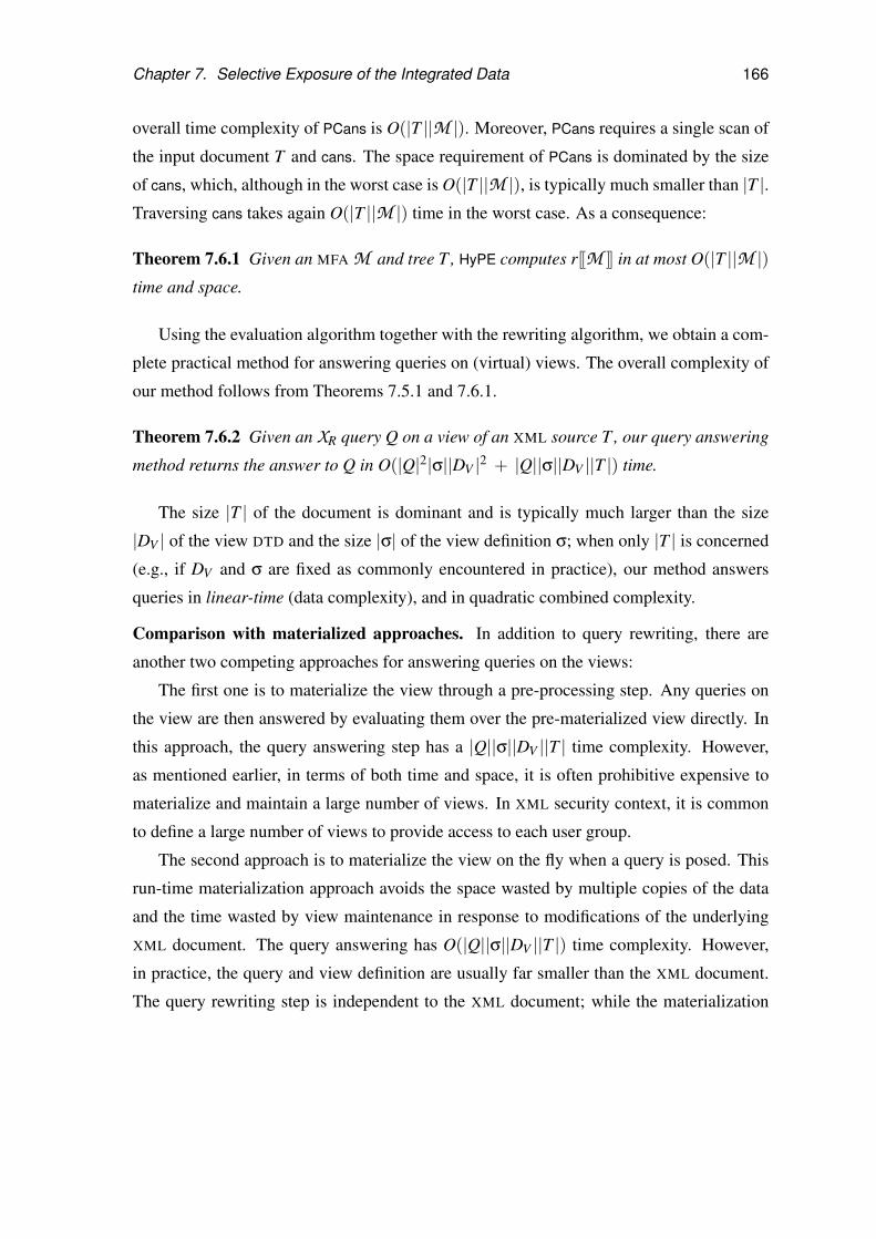
Chapter 7. Selective Exposure of the Integrated Data 166
overall time complexity of PCans is O(|T ||M |). Moreover, PCans requires a single scan of
the input document T and cans. The space requirement of PCans is dominated by the size
of cans, which, although in the worst case is O(|T ||M |), is typically much smaller than |T |.Traversing cans takes again O(|T ||M |) time in the worst case. As a consequence:
Theorem 7.6.1 Given an MFA M and tree T , HyPE computes r[[M ]] in at most O(|T ||M |)time and space.
Using the evaluation algorithm together with the rewriting algorithm, we obtain a com-
plete practical method for answering queries on (virtual) views. The overall complexity of
our method follows from Theorems 7.5.1 and 7.6.1.
Theorem 7.6.2 Given an XR query Q on a view of an XML source T , our query answering
method returns the answer to Q in O(|Q|2|σ||DV |2 + |Q||σ||DV ||T |) time.
The size |T | of the document is dominant and is typically much larger than the size
|DV | of the view DTD and the size |σ| of the view definition σ; when only |T | is concerned
(e.g., if DV and σ are fixed as commonly encountered in practice), our method answers
queries in linear-time (data complexity), and in quadratic combined complexity.
Comparison with materialized approaches. In addition to query rewriting, there are
another two competing approaches for answering queries on the views:
The first one is to materialize the view through a pre-processing step. Any queries on
the view are then answered by evaluating them over the pre-materialized view directly. In
this approach, the query answering step has a |Q||σ||DV ||T | time complexity. However,
as mentioned earlier, in terms of both time and space, it is often prohibitive expensive to
materialize and maintain a large number of views. In XML security context, it is common
to define a large number of views to provide access to each user group.
The second approach is to materialize the view on the fly when a query is posed. This
run-time materialization approach avoids the space wasted by multiple copies of the data
and the time wasted by view maintenance in response to modifications of the underlying
XML document. The query answering has O(|Q||σ||DV ||T |) time complexity. However,
in practice, the query and view definition are usually far smaller than the XML document.
The query rewriting step is independent to the XML document; while the materialization

Chapter 7. Selective Exposure of the Integrated Data 167
step needs to traverse the XML document multiple passes. This approach will inevitably
waste computations to generate and store the part of views which is irrelevant to answer
the query.
7.7 Optimizing Regular XPath Evaluation
Although HyPE already performs well in practice (see Section 7.8), we developed a novel
index structure which enables HyPE to skip even more subtrees. In the following, we denote
by OptHyPE the version of HyPE which is built on top of the index, and by OptHyPE-C the
version of HyPE which uses a compressed version of the index.
Given a query Q over a tree T , the secure sub-framework employs a novel index struc-
ture on T to decide whether HyPE can skip from visiting certain sub-trees of T . The in-
troduced index structure is capable of summarizing, at each node u, information regarding
all the nodes in the subtree that is rooted at u. In what follows, we first present the index
and then describe how it is used in optimization. We note that both the index structure
and our optimization technique are generic enough to be applicable in other contexts or
optimization efforts, not just for rewritten queries (MFA’s).
7.7.1 The Type-Aware XML (TAX) index
Of major concern in the optimization of XPath queries is to minimize the cost of the ‘//’
operator. To this end, various number indexing structures have been proposed that, given
two nodes u and w, they can answer in constant time whether node u is an ancestor of w.
One such scheme uses the pair of pre/post-order tree traversal numbers to annotate each
node [Die82]. Figure 7.12(a) shows an example of the index over a tree that conforms to a
simplified version of our hospital DTD. To save space, the simplified DTD only considers
hospitals, their patients, and each patient has visits that involve either a test or a medication.
In this scheme, a node u is an ancestor of w if u occurs before w in the preorder traversal and
after w in the postorder traversal. An alternative index was proposed in [LM01] in which
a node is annotated with the pair of preorder traversal and range numbers, where the latter
is the maximum number of descendants of the node. Figure 7.12(b) shows an example of
the order/range scheme, on the same tree as in Fig. 7.12(a). In the order/range index, u is
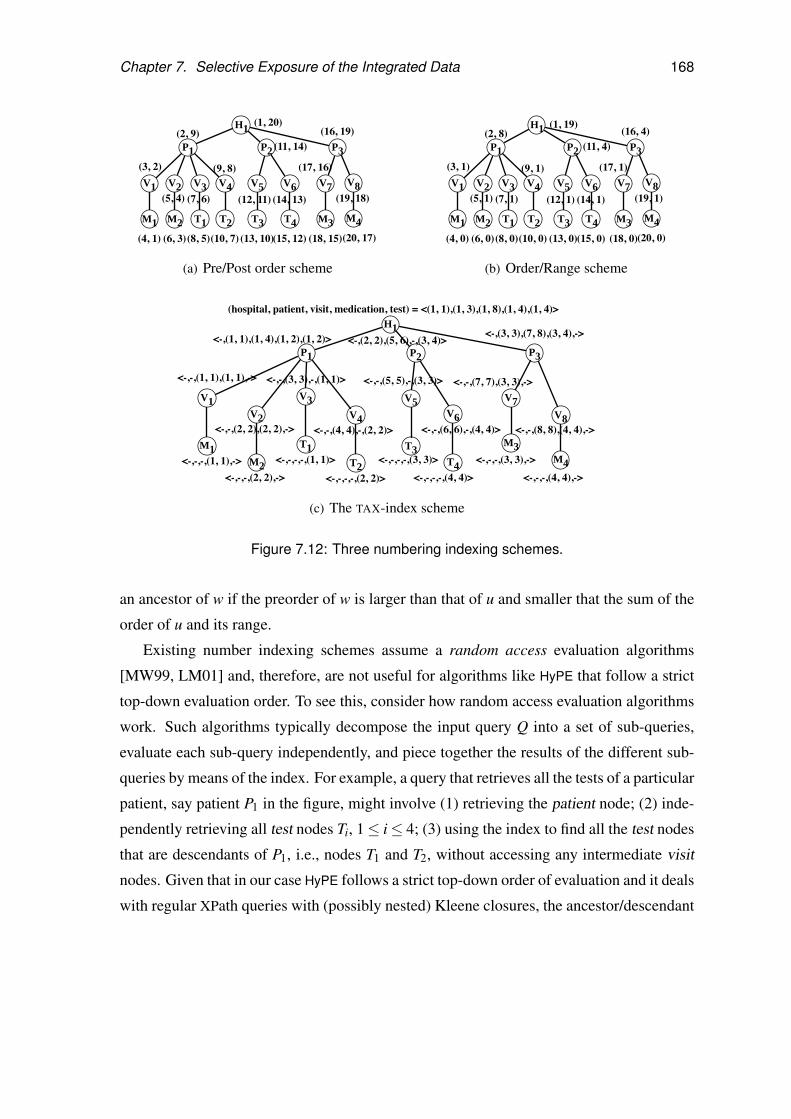
Chapter 7. Selective Exposure of the Integrated Data 168
H1
P1 P2
V3V2V1 V5 V6
M1 M2 T1 T3 T4
(1, 20)
(11, 14) (2, 9)
(4, 1)
(3, 2)
(6, 3)
(5, 4)
(8, 5)
(7, 6)
(13, 10)
(12, 11)
(15, 12)
(14, 13)
P3
V7 V8
M3 M4
(16, 19)
(18, 15)
(17, 16)
(20, 17)
V4
T2(10, 7)
(9, 8)
(19, 18)
(a) Pre/Post order scheme
H1
P1 P2
V3V2V1 V5 V6
M1 M2 T1 T3 T4
(1, 19)
(11, 4) (2, 8)
(4, 0)
(3, 1)
(6, 0)
(5, 1)
(8, 0)
(7, 1)
(13, 0)
(12, 1)
(15, 0)
(14, 1)
P3
V7 V8
M3 M4
(16, 4)
(18, 0)
(17, 1)
(20, 0)
V4
T2(10, 0)
(9, 1)
(19, 1)
(b) Order/Range scheme
H1
P1 P2
V3V2
V1 V5V6
M1M2
T1 T3T4
(hospital, patient, visit, medication, test) = <(1, 1),(1, 3),(1, 8),(1, 4),(1, 4)>
<-,(1, 1),(1, 4),(1, 2),(1, 2)> <-,(2, 2),(5, 6),-,(3, 4)>
<-,-,-,(1, 1),->
<-,-,-,(2, 2),->
<-,-,-,-,(1, 1)> <-,-,-,-,(3, 3)>
<-,-,-,-,(4, 4)>
<-,-,(6, 6),-,(4, 4)>
<-,-,(5, 5),-,(3, 3)> <-,-,(3, 3),-,(1, 1)>
<-,-,(2, 2),(2, 2),->
<-,-,(1, 1),(1, 1),->
P3
V7V8V4
T2<-,-,-,-,(2, 2)>
<-,-,(4, 4),-,(2, 2)>
<-,(3, 3),(7, 8),(3, 4),->
M3M4
<-,-,(7, 7),(3, 3),->
<-,-,(8, 8),(4, 4),->
<-,-,-,(3, 3),->
<-,-,-,(4, 4),->
(c) The TAX-index scheme
Figure 7.12: Three numbering indexing schemes.
an ancestor of w if the preorder of w is larger than that of u and smaller that the sum of the
order of u and its range.
Existing number indexing schemes assume a random access evaluation algorithms
[MW99, LM01] and, therefore, are not useful for algorithms like HyPE that follow a strict
top-down evaluation order. To see this, consider how random access evaluation algorithms
work. Such algorithms typically decompose the input query Q into a set of sub-queries,
evaluate each sub-query independently, and piece together the results of the different sub-
queries by means of the index. For example, a query that retrieves all the tests of a particular
patient, say patient P1 in the figure, might involve (1) retrieving the patient node; (2) inde-
pendently retrieving all test nodes Ti, 1≤ i≤ 4; (3) using the index to find all the test nodes
that are descendants of P1, i.e., nodes T1 and T2, without accessing any intermediate visit
nodes. Given that in our case HyPE follows a strict top-down order of evaluation and it deals
with regular XPath queries with (possibly nested) Kleene closures, the ancestor/descendant

Chapter 7. Selective Exposure of the Integrated Data 169
relation provided by the index is not very useful.
Another, rather surprising, thing to notice about existing number indexing schemes is
that the index of a tree T provides minimal information about the tree it indexes. Consider,
for example, the index entry of node H1 in Fig. 7.12(a). As long as the sub-tree rooted at
H1 consists of 19 nodes, the index entry of H1 remains unchanged. Just by looking at the
index of H1, we cannot tell whether this is the root of a tree with a single patient and eight
recorded visits or it has the structure of the tree shown in the figure. This does not meet
our expectation that an index provides at least some information about the indexed item, in
XML and in general.
In response to this we introduce a novel indexing structure that can be used both in strict
top-down evaluation algorithms, like HyPE, and in random access evaluation algorithms.
The index provides, at each node u, an accurate summary of the nodes that are in the
sub-tree rooted at u. Central to the summarization process is the simple observation that
different nodes in the tree have different types. To the best of our knowledge, all number
indexing schemes in the literature are type-agnostic, that is, they assigns numbers to nodes
but ignore the fact that different nodes have different types. However, it is natural to index
the nodes of each type separately and it is not a coincidence that in relational databases
we usually index each relation attribute (type) independently and we do not build one big
index for the whole relation.
We next present the Type-Aware XML index, or TAX-index for short. A TAX-index
essentially encapsulates as many indexes as there are types in the DTD. In the TAX-index,
for each node u in a tree T we maintain a vector Vu of size |Ele|, where Ele is the set of
types in the DTD D of T . We use Vu(E) to denote the element in vector Vu for type E ∈ Ele.
Each such element contains a pair of numbers and thus each node requires O(|Ele|) space
(we show how to compress the index shortly). Sometimes, an element is left without value.
In that case we put a dash in its position. Figure 7.12(c) shows an example of the index,
where |Ele|= 5 and the values of the vector are shown for each node.
We now explain how we assign values to the vector elements and the meaning of this
assignment. We assign identifiers to nodes of different types independently by numbering
all the nodes of a type in a preorder traversal of tree T . Consider a node u of type E and
assume that u is the ith node of type E encountered during the traversal. Then, Vu(E)[0] = i,
where Vu(E)[0] is the first entry of the Vn(E) element. The value of the second entry in the

Chapter 7. Selective Exposure of the Integrated Data 170
element is explained later. In Fig. 7.12(c), VP2(patient)[0] = 2 while VV2(visit)[0] = 2 Now,
consider element Vu(E ′) for node u, for any type E ′ other than E. In this element, we store
the smallest and largest identifier of nodes that are of type E ′ and belong to the subtree of T
rooted at u. In the figure, node P1 has VP1(visit) = (1,4) to indicate that the visit nodes with
identifiers from 1 to 4 are its descendants. Similarly, VP1(medication) = (1,2) to indicate
that medication nodes with identifiers 1 and 2 are descendants of the P1 node. One more
detail remains, concerning the value of the second entry in Vu(E). In this position, we store
the largest identifier of a node of type E that is a descendant of u. If the DTD is recursive, it is
possible that nodes of the same type are descendants of each other. Algorithm buildTAXIndex
(omitted due to space limitations) computes the vectors Vu for all the nodes u of a tree T via
a single traversal of the tree. In terms of space, a naive strategy would require O(|T ||Ele|)space. However, we can compress substantially the vector of each node. Indeed, for a
node u of type E, we only need to allocate space in the vector for the types that can be
descendants of E. Through static (offline) analysis of the DTD, we can determine which
these types are for each E. Using this optimization, for the TAX-index in Fig. 7.12(c), we
can save the space for almost all the dash (“-”) entries. Indeed, our experiments show that,
in spite of its added-value, the space requirements of a compressed TAX-index are at most
three times that of the corresponding order/range index over the same tree. In the following
section, we show how we can go one step further to compress the TAX-index even more.
A TAX-index summarizes, at each node, information regarding the subtree that is rooted
at that node. This is used in the next section to optimize the evaluation of XR queries. The
following proposition shows that a TAX-index can do more, namely, it can also be used to
answer ancestor/descendant queries.
Proposition 7.7.1: For any two nodes n and n′ of a tree T , n is an ancestor of n′ iff for each
E ∈ Ele, Vn(E)[0]≤Vn′(E)[0] and Vn(E)[1]≥Vn′(E)[1]. 2
7.7.2 The Optimization Algorithm
Our optimization algorithm, called OptHyPE, is built on top of the HyPE Algorithm. Al-
gorithm OptHyPE uses the TAX-index to reduce both the number of tree nodes visited by
the selection automaton N and the number of filters evaluated by the FA’s. To do this, the
algorithm first assumes that each state of both the selection SA N and the FA’s is annotated

Chapter 7. Selective Exposure of the Integrated Data 171
H1
P1 P2
V3V2
V1 V5V6
M1M2
T1 T3T4
(hospital, patient, visit, medication, test) = <0,1,1,1,1>
<0,1,1,1,1> <0,1,1,0,1>
<0,0,0,0,1>
<0,0,0,0,1> <0,0,0,0,1>
<0,0,0,1,0>
<0,0,0,1,0>
P3
V7V8V4
T2
<0,1,1,1,0>
M3M4
<0,0,0,1,0>
<0,0,0,1,0>
<0,0,0,0,1>
Figure 7.13: The TAXbit-index scheme
with the types of the elements that can reach this state. We are mainly interested in the
annotation of final states which identify, in the case of the SA N , the set EleN of element
types of nodes that can appear in the answer set.
Now, consider a query Q = hospital/patient/visit/medication, which returns all the
medication of the hospital patients. Then, EleN(Q) = {medication}. Using HyPE, we need
to access all the nodes in the tree shown in Fig. 7.12(c) in order to return the four medication
leaf nodes. However, we can use the information in the TAX-index to reduce the number
of node accesses as follows. Consider the phase in the HyPE during which we have already
visited the two left-most subtrees of the patient node P1. At this point, node P1 is at the
top of the stack and the two left-most medication leaf nodes M1 and M2 are already in the
potential answer set. Under normal execution, HyPE will add in the stack node V3 in order
to continue the evaluation of the remaining subtree that is rooted at P1. However, we know
from EleN(Q) that we are looking for medication nodes and we also know that we already
retrieved two such nodes in the subtree of P1. Furthermore, from the TAX-index entry of
P1, we know that P1 has only two such nodes as descendants. Thus, we need not evaluate
any other part of the subtree of P1 since we are sure that no more medication nodes exist.
This observation is used by our optimization algorithm to save four (unnecessary) node
accesses. Using similar reasoning, we save four more node accesses at node P2 since no
medication nodes are present in its subtree. Overall, our optimization algorithm performs,
in this example, 40% less node accesses than HyPE.
Interestingly enough, the same idea works for the evaluation of filters. For example,
consider the following query Q′ that returns all the patients for which there is some test,

Chapter 7. Selective Exposure of the Integrated Data 172
that is, Q′ = hospital/patient [visit/test]. We know that for the filter automaton A , EleA =
{test}. Again, using HyPE we need to evaluate the filter in 16 nodes (all the nodes in
the subtrees that are rooted at patient nodes). However, given the TAX-index entries for
nodes V1 and V2, we know that we do not need to visit any of their descendants since there
are no test nodes there. This observation is used by our optimization algorithm to save
two node accesses (the M1 and M2 nodes). Using similar reasoning, we save four more
node accesses by not evaluating the filter in the subtree rooted at node P3. Overall, our
optimization algorithm performs, in this example, 37.5% less node accesses than HyPE.
Briefly, we describe the implementation of OptHyPE (which is an extension of HyPE
and is omitted due to lack of space). We extend HyPE to maintain a global vector GV
which stores the summary of the visited nodes. For example, while evaluating query
Q above, and after visiting the two left-most subtrees of node P1, the vector is GV =
〈(1,1),(1,1),(1,2),(1,2),−〉, while GV is equal to 〈(1,1),(1,3),(1,6),(1,2),(1,4)〉 af-
ter visiting node P3 and before any of its descendants is accessed. During evaluation
in OptHyPE, vector GV is compared with the vector of the node at the top of the stack,
for example with that of node P1. Since we are looking for medication nodes, and since
GV (medication) = VP1(medication) (we already visited all the medication descendants of
P1), algorithm OptHyPE skips from visiting the remaining subtree of P1. The vector of P1 is
also used to update GV with information regarding the unvisited parts of the tree.
There is an alternative implementation of OptHyPE that results in significant space sav-
ings, in terms of the size of the index used, but may result in some additional node accesses.
Briefly, notice that in our optimization algorithm it often suffices to know that a descen-
dant of a particular type exists, or not. Since we are not interested (at least in HyPE) in
ancestor/descendant queries, we can use a variation of the TAX-index, called TAXbit-index
and shown in Fig. 7.13, which only uses a single bit in entry Vu(E) of a node u to indicate
whether node u has a descendant of type E. It is not hard to see that we can still use the
index while evaluating the query Q above. Assuming that we have already visited the two
left-most subtrees of P1, we need to descent to node V3 before we realize that no medication
nodes exist there. We still save the cost of visiting the subtree rooted at P2 since we already
know that no medication nodes exist there. Overall, for this example, we perform 37.5%
less node accesses than HyPE.

Chapter 7. Selective Exposure of the Integrated Data 173
14
12
10
8
6
4
2
7063564942352821147
Tim
e (s
ec)
Document size (MB)
JAXPHyPE
OptHyPEOptHyPE-C
(a) A filter returning a large set of nodes
14
12
10
8
6
4
2
7063564942352821147
Tim
e (s
ec)
Document size (MB)
JAXPHyPE
OptHyPEOptHyPE-C
(b) Query with filter conjunctions
16
14
12
10
8
6
4
2
7063564942352821147
Tim
e (s
ec)
Document size (MB)
JAXPHyPE
OptHyPEOptHyPE-C
(c) Query with filter disjunctions
Figure 7.14: XPath query evaluation times
7.8 Experimental Study
We have developed a prototype system SMOQE [FGJK06] supporting MFA’s and algo-
rithms rewrite and HyPE (and its variants OptHyPE and OptHyPE-C). In our experiments,
we focused on the most time-consuming module of SMOQE, i.e., the query evaluator. The
experiments were conducted on a dual 2.3GHz Apple Xserve with 4GB of memory. For the
generation of our datasets, we used ToXGene [BMKL02]. We generated XML documents
that conform to our recursive hospital DTD shown in Fig. 7.1, with sizes ranging from 7MB
to 70MB, in 7MB increments. Each increment roughly corresponds to adding the medical
history of 10,000 patients to our document tree. Therefore, the largest document stores
the medical history of approximately 100,000 patients. The maximal depth of the trees
is 13. The generated data consist mainly of element nodes, and to a lesser extent of text
nodes. Therefore, the size of the document has a direct impact on query evaluation. For
example, our smallest document (7MB) consists of 303,714 element nodes vs 151,187 text
nodes. The text nodes are used to increase the selectivity of queries but their size is kept to

Chapter 7. Selective Exposure of the Integrated Data 174
2018161412108642
7063564942352821147
Tim
e (s
ec)
Document size (MB)
HyPEOptHyPE
OptHyPE-C
(a) Kleene star outside filter
16
14
12
10
8
6
4
2
7063564942352821147
Tim
e (s
ec)
Document size (MB)
HyPEOptHyPE
OptHyPE-C
(b) Filter inside Kleene star
10
8
6
4
2
7063564942352821147
Tim
e (s
ec)
Document size (MB)
HyPEOptHyPE
OptHyPE-C
(c) Kleene star in filter
Figure 7.15: regular XPath query evaluation times
a minimum (so as not to increase the document size).
Using the generated document trees, we conducted two sets of experiments, one regard-
ing XPath evaluation, the other regarding regular XPath. The reported times are averaged
over at least 5 runs of each experiment.
Evaluating XPath Queries. Since regular XPath subsumes XPath, we investigate the per-
formance of HyPE and its variants for the evaluation of XPath queries.
We compared our performance with that of the Java API for XML Processing Refer-
ence Implementation (JAXP RI 1.3), which relies on XERCES and XALAN [XX]. We also
compared with JAXP-COMPILE, a version of JAXP that pre-compiles the input query and
converts it into a set of Java classes. The two JAXP versions had similar performance and
thus we only report one of them.
We ran various types of XPath queries with simple filters on data values, unions of
queries, and Boolean combinations of filters. Figure 7.14 shows the evaluation time for
three different types of XPath queries. We show the evaluation time both for queries with
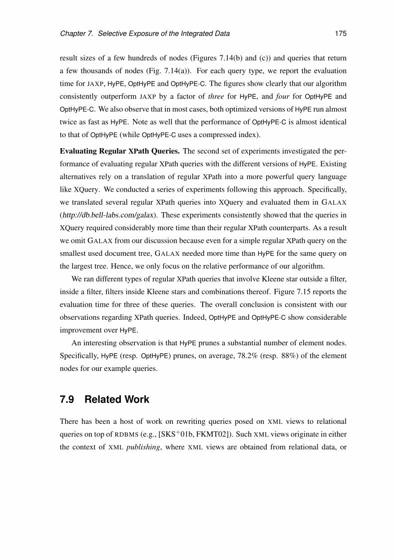
Chapter 7. Selective Exposure of the Integrated Data 175
result sizes of a few hundreds of nodes (Figures 7.14(b) and (c)) and queries that return
a few thousands of nodes (Fig. 7.14(a)). For each query type, we report the evaluation
time for JAXP, HyPE, OptHyPE and OptHyPE-C. The figures show clearly that our algorithm
consistently outperform JAXP by a factor of three for HyPE, and four for OptHyPE and
OptHyPE-C. We also observe that in most cases, both optimized versions of HyPE run almost
twice as fast as HyPE. Note as well that the performance of OptHyPE-C is almost identical
to that of OptHyPE (while OptHyPE-C uses a compressed index).
Evaluating Regular XPath Queries. The second set of experiments investigated the per-
formance of evaluating regular XPath queries with the different versions of HyPE. Existing
alternatives rely on a translation of regular XPath into a more powerful query language
like XQuery. We conducted a series of experiments following this approach. Specifically,
we translated several regular XPath queries into XQuery and evaluated them in GALAX
(http://db.bell-labs.com/galax). These experiments consistently showed that the queries in
XQuery required considerably more time than their regular XPath counterparts. As a result
we omit GALAX from our discussion because even for a simple regular XPath query on the
smallest used document tree, GALAX needed more time than HyPE for the same query on
the largest tree. Hence, we only focus on the relative performance of our algorithm.
We ran different types of regular XPath queries that involve Kleene star outside a filter,
inside a filter, filters inside Kleene stars and combinations thereof. Figure 7.15 reports the
evaluation time for three of these queries. The overall conclusion is consistent with our
observations regarding XPath queries. Indeed, OptHyPE and OptHyPE-C show considerable
improvement over HyPE.
An interesting observation is that HyPE prunes a substantial number of element nodes.
Specifically, HyPE (resp. OptHyPE) prunes, on average, 78.2% (resp. 88%) of the element
nodes for our example queries.
7.9 Related Work
There has been a host of work on rewriting queries posed on XML views to relational
queries on top of RDBMS (e.g., [SKS+01b, FKMT02]). Such XML views originate in either
the context of XML publishing, where XML views are obtained from relational data, or

Chapter 7. Selective Exposure of the Integrated Data 176
in the context of XML storage, where XML views reflect XML data stored in a relational
database. In both contexts, XML queries on the XML view need to be translated into SQL.
Even in this setting, recursion in the view DTD makes the translation challenging. As
observed by [KKN04], most of the existing approaches cannot translate recursive queries
over recursive views (two exceptions are [SKS+01b, FYL+05]).
There has been little work on query rewriting for XML views in the native XML setting
where one does not rely on any RDBMS, i.e., the setting considered in this chapter. [PA05]
concentrates on views in XML integration context, while [FCG04] and [BF05] in XML
security context. [PA05] investigates the query answering on XML views defined in local-
as-view (LAV) approach with constraints on global schema. The view and the query are
specified in a so called prefix-selection query language which is base on homomorphism
between trees that preserves root, parent-child relationships and labeling. The filters in
XPath can be expressed in the language, but recursive axes such as descendant axis can
not. Polynomial time (data complexity) query answering algorithm is developed based on
constructing a weak representation system to represent all legal XML instance over global
schema under the view definition (i.e. the mappings from global schema to source schema
as well as the constraints on global schema). [BF05] studies the closure properties and al-
gorithms for the query rewriting (called query composition there) of several fragments of a
subtree query language for views defined in global-as-view (GAV) approach. The language
is defined by modifying the semantics of XPath fragments. The largest fragment studied
in [BF05] is syntactically comparable to the XPath fragment X studied in this chapter with
extension to upward axes. The motivation of their language is to give a convenient way
for specifying certain subtree queries. It can not express the views defined in this chapter
which hide certain ancestors of some nodes in the view — the views defined by [BF05]
always have the same root-to-leaf paths as the underlying document. Their query rewriting
algorithm runs in polynomial time in the size of the queries, under the assumption of nor-
malization (for un-normalized queries, there is a provable exponential blow-up). [FCG04]
studies the query rewriting algorithms for the views defined similarly as ours. It shows that
X is closed under query rewriting for non-recursive XML views. Our rewriting algorithm in
this chapter gives a practical solution to rewriting queries in XPath and its extension regular
XPath over recursive XML views which can hide arbitrary XML nodes.
The research on XML access control enforcement could be classified as either static

Chapter 7. Selective Exposure of the Integrated Data 177
mechanism which enforces access policies at compile-time of the query evaluation or dy-
namic mechanism which enforces them at run-time of the query evaluation. In a compile-
time approach, the access policies are embedded into queries. The access control enforce-
ment is typically achieved by either query filtering where the part of queries that returns un-
authorized information is filtered out, or query rewriting where the accessible information
is explicit defined for authorized users as virtual views. [MTKH06, LLLL04] take query
filtering approach. Both of them use automata to represent access policies. In [LLLL04]
the policies are embedded into the queries by evaluating the queries on the automata that
represent the policies. In [MTKH06], besides the policies, the queries and schemas, if
available, are also represented by automata. Then the automata represented queries are
compared with the automata represented policies and schemas. If the queries are partially
granted, a run-time checking is still needed. As mentioned in Section 7.1, [FCG04] fol-
lows query rewriting approach. A view definition and a view schema are explicitly derived
from the security policies. The query on the view is then unfolded to incorporate the view
definition.
In a run-time approach, the access policies are associated with XML documents. A
naıve way to achieve the association is to annotate (also called label), each node in XML
documents with security properties such as the user groups/roles that can access the node.
These annotated documents could be prohibitively large because the user groups/roles and
access actions are appended in every nodes. A host of research [YSLJ04, JF05, ZZSZ07]
focuses on compressing the annotated documents and supporting queries on them. The
compressing is usually done by utilizing access locality. Access locality is the property
that the adjacent nodes in an XML tree tend to have the same access policies. Thus,
it is not necessary to annotate every node in an XML tree and the annotated documents
could be represented compactly. In [YSLJ04, JF05], the compact representation is called
Compressed Accessibility Maps (CAMs) where the adjacency is defined by the ancestor-
descendant relationship. In [ZZSZ07], it is called Document Ordered Labelling (DOL),
where the adjacency is defined by document order. Although the compression reduced
the space consumption, the mixture of XML instance and security properties and the time
required to compute the compression are still disadvantages of the run-time approach. In
many cases, the compile-time approach is preferred because the XML documents, which are
usually large in database applications, are not touched. A critical problem in the compile-

Chapter 7. Selective Exposure of the Integrated Data 178
time approach is query rewriting on XML views, which is a focus of this chapter. More
work on XML access control can be found in a survey [FM04].
In [Mar04b], regular XPath was introduced and it was shown that a regular XPath query
Q can be evaluated over an XML tree T in O(|Q||T |) time, requiring multiple passes over the
document tree. A two-pass algorithm for XPath was developed in [Koc03], but it cannot be
easily extended to deal with the Kleene star. As already observed in Section 7.6, even when
only XPath is concerned, our evaluation algorithm, HyPE, does not need a pre-processing
step (another scan of T ) that is required by the algorithm of [Koc03], and is more effective
in pruning irrelevant nodes when traversing T , among other things.
Several automaton formalisms were proposed for processing multiple XPath queries on
streaming XML (e.g. [DFFT02, GGM+04]). The idea of AFA was explored by [GGM+04]
for evaluating XPath filters. However, no previous work has attempted to characterize
regular XPath in terms of both NFA and AFA in an integrated automaton.
Another line of research concerns view-based query rewriting and answering
(see [Hal01] for a survey). Here, given a set of (materialized) views and a query Q on
the underlying database, the goal is to answer Q solely on the basis of the views. The prob-
lem we consider here is the opposite scenario where the query Q is posed on the view, and
it is to find a rewriting Q′ of Q on the underlying document.

Chapter 8
Conclusions and Future Directions
With the increasing complexities of the data in real world organizations and the advancing
technologies to manage the data, information systems need to be enhanced in several di-
mensions. For instance, in data dimension, the systems need to cope with both structured
data and semi-structured data. In service dimension, beyond storing and querying large vol-
ume of data, the systems need to provide functionalities to improve the quality of the data,
integrate the data from heterogeneous sources and protect the data against unauthorized
access. In response to these challenges, this thesis presents a comprehensive framework,
referred to as CLINSE, to clean, integrate and secure data by leveraging both relational and
XML data management techniques.
In CLINSE, three sub-frameworks have been proposed. First, the inconsistencies in the
data residing in each relational data source are detected and repaired in the data cleaning
sub-framework. Second, the relational data is published into XML format and integrated
with other XML data sources guided by a predefined schema in the data integration sub-
framework. At last, the integrated XML data is protected by a security sub-framework
which hides the integrated data, but exposes a virtual XML view for each user group and
supports query answering on these views.
Data cleaning sub-framework. To clean the data stored in relational databases, the thesis
has introduced CFDs as an extension of FDs, and shown that CFDs are capable of capturing
inconsistencies beyond what traditional FDs can detect. To apply CFDs in data cleaning,
SQL-based techniques for detecting violations of CFDs have been proposed and experi-
mentally evaluated. These results, together with the static analysis reported in [BFG+07],
179

Chapter 8. Conclusions and Future Directions 180
establish a constraint-based model for data cleaning.
In CLINSE, based on CFDs, a sub-framework for improving data quality has been pro-
posed. It is shown that while CFDs are more appropriate for data cleaning than traditional
FDs, they make our lives harder when developing (semi-)automated data-cleaning meth-
ods based on CFDs. Indeed, previous methods based on FDs may not even terminate when
applied to CFDs. It is shown that based on CFDs, the problem for finding optimal repairs
and the problem for incrementally finding optimal repairs are both NP-complete. In light
of these intractability results, heuristic algorithms for both problems have been developed
in CLINSE framework. Moreover, their effectiveness and efficiency in improving the con-
sistency of the data have been experimentally verified. This work is the first effort to
(incrementally) clean data based on conditional constraints.
Data integration sub-framework. To integrate data, a novel language, XIGs, has been
proposed for specifying XML integration. XIGs automatically support conformance to a
target DTD. They allow one to build a large, complex integration via composition of com-
ponent XIGs. Novel optimization algorithms for evaluating XIGs have also been developed.
These lead to a design tool and a user/application-level interface for XQuery to facilitate
schema-directed XML integration.
Data security sub-framework. To secure the XML data, a sub-framework for efficiently
answering regular XPath queries posed on possibly recursively defined XML views has been
provided. On the theoretical side, results have been established for the closure property and
complexity of rewriting (regular) XPath queries on views into (regular) XPath queries on the
source. On the practical side, a practical approach has been proposed for query rewriting,
by using MFA as an intermediate representation of rewritten regular XPath queries. The
novelty of the approach consists in (a) an algorithm for rewriting regular XPath queries on
XML views to equivalent MFA on the source, and (b) an efficient evaluation algorithm for
MFA. These yield an effective method for answering queries posed on XML views of XML
data, and are useful in enforcing XML access control, among other things. Furthermore,
the evaluation algorithm is among the first for efficiently processing regular XPath queries.
A prototype system supporting all these algorithms has been fully implemented, and the
experimental results verified the efficiency of these techniques.
There is much more to be done.

Chapter 8. Conclusions and Future Directions 181
XML data cleaning. In the current framework, only the data in relational sources is
cleaned before integration. However, the data in other sources, especially XML sources,
may contain errors and need to be cleaned too. More importantly, the data integration
process may also introduce dirty data due to the mis-translation and incompatibility of the
semantics of the source data. Therefore, XML data cleaning is definitely needed in this
framework. Beyond CLINSE framework, XML data cleaning tools are valuable in cleaning
the data extracted from the Web, such as address data. Although the constraints for XML
data cleaning could be defined as assertions in Schematron [ISO06a], how to check the
consistencies of these assertions and use them to detect and repair XML data are still open
problems.
Other conditional constraints for relational data. To clean relational data, constraints
beyond CFDs are certainly needed. For example, data cleaning based on both CFDs and con-
ditional inclusion dependencies, which are defined along the same lines as CFDs, needs to
be studied. The static analysis of these conditional dependencies becomes, however, more
intriguing. In particular, the consistency and implication problems for these conditional
constraints become undecidable. To cope with this it is necessary to find effective and effi-
cient heuristic algorithms for the consistency and implication analyses of these conditional
constraints.
Improve constraint-based data cleaning by profiling the data. Automated methods
for discovering CFDs and conditional inclusion dependencies are certainly an interesting
topic. It is nontrivial to identify all sensible pattern tuples without over-populating pattern
tableaux. Probably, a more general question is whether constraint-based data cleaning and
data profiling could be combined to provide better results. For example, in constraint-based
data cleaning, the inconsistent data may also contain clean data. Currently, cost models are
used to decide which part of the inconsistent data is dirty. On the other hand, the outliers
discovered in data profiling could be correct data. However, if part of the inconsistent
data detected by constraint-based data cleaning is among these outliers, it is more likely
to be dirty. Moreover, the repair suggestions in data profiling could be validated by the
constraints. Although such mutual verification is feasible in principle, its effects in practice
and the choice of constraints and outlier models are topics to be explored.
XML views on heterogeneous data. In CLINSE framework, XIGs are used to specify

Chapter 8. Conclusions and Future Directions 182
XML views over XML data. The data under other models needs to be published into XML
format before the integration. A simplification of this process would be to incorporate
XML publishing features into XIGs. Extending XIGs to allow both XQuery and SQL to be
associated with productions of the target DTDs would enable XIGs to define XML views
over heterogeneous data, but how to cope with both the tree valued attributes and tuple
valued attributes, and how to optimize the evaluation of the extended XIGs are challenging
problems. Another direction for improving XIGs is to identify practical XQuery fragments
that allow efficient optimization techniques and termination analyses for XIGs.
XML Query rewriting in other contexts. In this thesis, (regular) XPath query rewriting
in security context is studied. It is interesting to extend this work to other contexts and
other XML query languages, such as, how to rewrite queries over XML views of multiple
XML data sources as found in data integration, and how to extend the rewriting algorithms
to handle queries and views specified in XQuery.

Bibliography
[AAR96] Andreas Arning, Rakesh Agrawal, and Prabhakar Raghavan. A linearmethod for deviation detection in large databases. In Knowledge Discoveryand Data Mining, pages 164–169, 1996.
[ABC99] Marcelo Arenas, Leopoldo E. Bertossi, and Jan Chomicki. Consistent queryanswers in inconsistent databases. In Proc. Symp. on Principles of DatabaseSystems (PODS), pages 68–79, 1999.
[ABC01] Marcelo Arenas, Leopoldo E. Bertossi, and Jan Chomicki. Scalar aggrega-tion in fd-inconsistent databases. In Proc. of Int’l Conf. on Database Theory(ICDT), 2001.
[ABC+03a] S. Abiteboul, A. Bonifati, G. Cobena, I. Manolescu, and T. Milo. DynamicXML documents with distribution and replication. In Proc. Int’l Conf. onManagement of Data (SIGMOD), 2003.
[ABC03b] Marcelo Arenas, Leopoldo Bertossi, and Jan Chomicki. Answer sets forconsistent query answering in inconsistent databases. Theory and Practiceof Logic Programming, 3(4):393–424, 2003.
[ABC+03c] Marcelo Arenas, Leopoldo Bertossi, Jan Chomicki, Xin He, Vijay Raghavan,and Jeremy Spinrad. Scalar aggregation in inconsistent databases. Theoreti-cal Computer Science (TCS), 296(3):405–434, 2003.
[Abi99] Serge Abiteboul. On views and XML. In Proc. Symp. on Principles ofDatabase Systems (PODS), 1999.
[AHV95] Serge Abiteboul, Richard Hull, and Victor Vianu. Foundations of Databases.Addison-Wesley, 1995.
[AL05] Macelo Arenas and Leonid Libkin. XML data exchange: Consistency andquery answering. In Proc. Symp. on Principles of Database Systems (PODS),2005.
[AMN+01a] Noga Alon, Tova Milo, Frank Neven, Dan Suciu, and Victor Vianu. Type-checking XML views of relational databases. In Proc. Symp. on Logic inComputer Science, 2001.
183

Bibliography 184
[AMN+01b] Noga Alon, Tova Milo, Frank Neven, Dan Suciu, and Victor Vianu. XMLwith data values: Typechecking revisited. In Proc. Symp. on Principles ofDatabase Systems (PODS), 2001.
[BBFL05] Leopoldo Bertossi, Loreto Bravo, Enrico Franconi, and Andrei Lopatenko.Fixing inconsistent databases by updating numerical attributes. In Proc. ofInt’l Workshop on Database and Expert Systems Applications, pages 854–858, 2005.
[BC03] Leopoldo Bertossi and Jan Chomicki. Query answering in inconsistentdatabases. In Logics for Emerging Applications of Databases, pages 43–83,2003.
[BCF+02] Michael Benedikt, Chee Yong Chan, Wenfei Fan, Rajeev Rastogi, ShihuiZheng, and Aoying Zhou. DTD-directed publishing with attribute translationgrammars. In Proc. of Int’l Conf. on Very Large Databases (VLDB), pages838–849, 2002.
[BCF+03] Michael Benedikt, Chee Yong Chan, Wenfei Fan, Juliana Freire, and Ra-jeev Rastogi. Capturing both types and constraints in data integration. InProc. Int’l Conf. on Management of Data (SIGMOD), pages 277–288, 2003.
[BCF04] Philip Bohannon, Byron Choi, and Wenfei Fan. Incremental evaluation ofschema-directed XML publishing. In Proc. Int’l Conf. on Management ofData (SIGMOD), pages 503–514, 2004.
[Ber06] Leopoldo Bertossi. Consistent query answering in databases. SIGMODRecord, 35(2):68–76, 2006.
[Ber07] Anders Berglund et al. XML Path Language (XPath) 2.0. W3C Recommen-dation, April 2007. http://www.w3.org/TR/xpath20/.
[BF05] Michael Benedikt and Irini Fundulaki. Xml subtree queries: Specificationand composition. In Proc. of Int’l Workshop on Database ProgrammingLanguages (DBPL), pages 138–153, 2005.
[BFFR05] Philip Bohannon, Michael Flaster, Wenfei Fan, and Rajeev Rastogi. A cost-based model and effective heuristic for repairing constraints by value mod-ification. In Proc. Int’l Conf. on Management of Data (SIGMOD), pages143–154, 2005.
[BFG+07] Philip Bohannon, Wenfei Fan, Floris Geerts, Xibei Jia, and Anastasios Ke-mentsietsidis. Conditional functional dependencies for data cleaning. InProc. of Int’l Conf. on Data Engineering (ICDE), pages 746–755, 2007.

Bibliography 185
[BFK05] Michael Benedikt, Wenfei Fan, and Gabriel Kuper. Structural properties ofXPath fragments. Theoretical Computer Science (TCS), 336(1):3–31, May2005.
[BFMV00] Luc Bouganim, Franoise Fabret, C. Mohan, and Patrick Valduriez. Dynamicquery scheduling in data integration systems. In Proc. of Int’l Conf. on DataEngineering (ICDE), 2000.
[BFV96] Luc Bouganim, Daniela Florescu, and Patrick Valduriez. Dynamic load bal-ancing in hierarchical parallel database systems. In Proc. of Int’l Conf. onVery Large Databases (VLDB), 1996.
[BGH03] Agnes Boskovitz, Rajeev Gore, and Markus Hegland. A logical formalisa-tion of the fellegi-holt method of data cleaning. In Proc. of Int’l Conf. onAdvances in Intelligent Data Analysis (IDA), pages 554–565, 2003.
[BGK+02] Philip Bohannon, Sumit Ganguly, Henry F. Korth, P. P. S. Narayan, andPradeep Shenoy. Optimizing view queries in ROLEX to support navigableresult trees. In Proc. of Int’l Conf. on Very Large Databases (VLDB), pages119–130, 2002.
[BGL+00] Chaitanya Baru, Amarnath Gupta, Bertram Ludascher, Richard Marciano,Yannis Papakonstantinou, Pavel Velikhov, and Vincent Chu. XML-basedinformation mediation with MIX. In Proc. Int’l Conf. on Management ofData (SIGMOD), 2000.
[BH92] Ravi Boppana and Magnu;s M. Halldorsson. Approximating maximum in-dependent sets by excluding subgraphs. BIT, 32(2):180–196, 1992.
[BK06] Michael Benedikt and Christoph Koch. XPath leashed. Unpublished survey,2006.
[BKMW01] Anne Brggemann-Klein, Makoto Murata, and Derick Wood. Regular treeand regular hedge languages over unranked alphabets: Version 1. Techni-cal Report HKUST-TCSC-2001-0, The Hongkong University of Science andTechnology, 2001.
[BMKL02] Denilson Barbosa, Alberto O. Mendelzon, John Keenleyside, and Kelly A.Lyons. Toxgene: An extensible template-based data generator for XML. InProc. of Int’l Workshop on the Web and Databases, 2002.
[BP85] Donald P. Ballou and Harold L. Pazer. Modeling data and process qual-ity in multi-input, multi-output information systems. Management Science,31(2):150–162, 1985.

Bibliography 186
[BP05] Andrey Balmin and Yannis Papakonstantinou. Storing and querying XMLdata using denormalized relational databases. The VLDB Journal, 14(1):30–49, March 2005.
[BPSM98a] Tim Bray, Jean Paoli, and C. M. Sperberg-McQueen. ExtensibleMarkup Language (XML) 1.0. W3C Recommendation, February 1998.http://www.w3.org/TR/REC-xml/.
[BPSM98b] Tim Bray, Jean Paoli, and C. M. Sperberg-McQueen. ExtensibleMarkup Language (XML) 1.0. W3C Recommendation, February 1998.http://www.w3.org/TR/REC-xml/.
[BS01] Renato Bruni and Antonio Sassano. Errors detection and correction in largescale data collecting. In Proc. of Int’l Conf. on Advances in Intelligent DataAnalysis (IDA), pages 84–94, 2001.
[CAYLS02] S. Cho, S. Amer-Yahia, L.V.S. Lakshmanan, and D. Srivastava. Optimizingthe secure evaluation of twig queries. In Proc. of Int’l Conf. on Very LargeDatabases (VLDB), 2002.
[CB00] Alexander Celle and Leopoldo E. Bertossi. Querying inconsistent databases:Algorithms and implementation. In Computational Logic, pages 942–956,2000.
[CD99] James Clark and Steve DeRose. XML Path Language (XPath) Version 1.0.W3C Recommendation, November 1999. http://www.w3.org/TR/xpath.
[CDSS98] Sophie Cluet, Claude Delobel, Jerome Simeon, and Katarzyna Smaga. Yourmediators need data conversion! In Proc. Int’l Conf. on Management of Data(SIGMOD), 1998.
[CFG+07] Gao Cong, Wenfei Fan, Floris Geerts, Xibei Jia, and Shuai Ma. Improvingdata quality: Consistency and accuracy. In Proc. of Int’l Conf. on Very LargeDatabases (VLDB), 2007.
[CFI+00] Michael J. Carey, Daniela Florescu, Zachary G. Ives, Ying Lu, JayavelShanmugasundaram, Eugene J. Shekita, and Subbu N. Subramanian.XPERANTO: Publishing object-relational data as XML. In Proc. of Int’lWorkshop on the Web and Databases, 2000.
[CFJK04] Byron Choi, Wenfei Fan, Xibei Jia, and Arek Kasprzyk. A uniform systemfor publishing and maintaining XML data. In Proc. of Int’l Conf. on VeryLarge Databases (VLDB), pages 1301–1304, 2004. Demo.
[CFR06] Don Chamberlin, Daniela Florescu, and Jonathan Robie. XQuery updatefacility. W3C Working Draft, July 2006. http://www.w3.org/TR/xqupdate/.

Bibliography 187
[Cha07] Don Chamberlin et al. XQuery 1.0: An xml query language. W3C Recom-mendation, January 2007. http://www.w3.org/TR/xquery.
[Che98] Bor-Chung Chen. Set-covering algorithms in edit generation. In Proc. theSection on Statistical Computing, American Statistical Association, 1998.
[Cho02] Byron Choi. What are real DTDs like. In Proc. of Int’l Workshop on the Weband Databases, 2002.
[Cho06] Jan Chomicki. Invited paper: Consistent query answering: Opportunitiesand limitations. In Proc. of Int’l Workshop on Database and Expert SystemsApplications, pages 527–531, 2006.
[Cho07] Jan Chomicki. Consistent query answering: Five easy pieces. In Proc. ofInt’l Conf. on Database Theory (ICDT), pages 1–17, 2007.
[CKS+00] Michael J. Carey, Jerry Kiernan, Jayavel Shanmugasundaram, Eugene J.Shekita, and Subbu N. Subramanian. XPERANTO: Middleware for pub-lishing object-relational data as XML documents. In Proc. of Int’l Conf. onVery Large Databases (VLDB), 2000.
[Cla99] James Clark. XSL Transformations (XSLT) Version 1.0. W3C Recommen-dation, November 1999. http://www.w3.org/TR/xslt.
[CLR03] Andrea Cali, Domenico Lembo, and Riccardo Rosati. On the decidabil-ity and complexity of query answering over inconsistent and incompletedatabases. In Proc. Symp. on Principles of Database Systems (PODS), 2003.
[CM01] James Clark and MURATA Makoto. RELAX NG Specification. OA-SIS Committee Specification and ISO/IEC 19757-2, December 2001.http://www.oasis-open.org/committees/relax-ng/spec-20011203.html.
[CM05] J. Chomicki and J. Marcinkowski. Minimal-change integrity maintenanceusing tuple deletions. Inf. Comput., 197:90–121, 2005.
[CM07] Balder ten Cate and Maarten Marx. Axiomatizing the logical core of XPath2.0. In Proc. of Int’l Conf. on Database Theory (ICDT), pages 134–148,2007.
[CMS04] Jan Chomicki, Jerzy Marcinkowski, and Slawomir Staworko. Comput-ing consistent query answers using conflict hypergraphs. In Proc. of Int’lConf. on Information and Knowledge Management (CIKM), pages 417–426,2004.
[CRF03] W. Cohen, P. Ravikumar, and S. Feinberg. A comparison of string-distancemetrics for name-matching tasks. In IIWeb, 2003.

Bibliography 188
[CT04] John Cowan and Richard Tobin. Xml information set (second edition). W3CRecommendation, February 2004.http://www.w3.org/TR/xml-infoset/.
[DdVPS00] E. Damiani, S.D.C di Vimercati, S. Paraboschi, and P. Samarati. SecuringXML documents. In Proc. of Int’l Conf. on Extending Database Technology(EDBT), 2000.
[DEGV01] Evgeny Dantsin, Thomas Eiter, Georg Gottlob, and Andrei Voronkov. Com-plexity and expressive power of logic programming. ACM Comput. Surv.,33(3):374–425, 2001.
[DESR03] Katica Dimitrova, M. EL-Sayed, and E. Rundensteiner. Order-sensitive viewmaintenance of materialized XQuery views. In ER, 2003.
[DFFT02] Yanlei Diao, Peter M. Fischer, Michael J. Franklin, and Raymond To. YFil-ter: Efficient and scalable filtering of XML documents. In Proc. of Int’lConf. on Data Engineering (ICDE), 2002.
[DFS99] Alin Deutsch, Mary Fernandez, and Dan Suciu. Storing semistructured datawith STORED. In Proc. Int’l Conf. on Management of Data (SIGMOD),pages 431–442, 1999.
[Die82] Paul F. Dietz. Maintaining order in a linked list. In SODA, 1982.
[DT01] Alin Deutsch and Val Tannen. Answering XML queries over heterogeneousdata sources. In Proc. of Int’l Conf. on Very Large Databases (VLDB), 2001.
[DT03] Alin Deutsch and Val Tannen. MARS: A system for publishing XML frommixed and redundant storage. In Proc. of Int’l Conf. on Very Large Databases(VLDB), 2003.
[dW96] Ton de Waal. Cherrypi: A computer program for automatic edit and im-putation. In UN/ECE Work Session on Statistical Data Editing, Voorburg.,1996.
[DW97] Lisa R. Draper and William E. Winkler. Balancing and ratio editing with thenew SPEER system. Technical report, U.S.Bureau of the Census, 1997.
[EBI] EBI. Gene Ontology. http://www.geneontology.org/.
[Eck02] Wayne Eckerson. Data Quality and the Bottom Line: Achiev-ing Business Success through a Commitment to High QualityData. Technical report, The Data Warehousing Institute, 2002.http://www.tdwi.org/research/display.aspx?ID=6064.

Bibliography 189
[EZ76] Andrzej Ehrenfeucht and H. Paul Zeiger. Complexity measures for regularexpressions. J. Comput. Syst. Sci. (JCSS), 12(2):134–146, 1976.
[FCG04] Wenfei Fan, Chee Yong Chan, and Minos Garofalakis. Secure XML query-ing with security views. In Proc. Int’l Conf. on Management of Data (SIG-MOD), 2004.
[FFM05] Ariel Fuxman, Elham Fazli, and Renee J. Miller. Conquer: efficient manage-ment of inconsistent databases. In Proc. Int’l Conf. on Management of Data(SIGMOD), pages 155–166, 2005.
[FGJK06] Wenfei Fan, Floris Geerts, Xibei Jia, and Anastasios Kementsietsidis.SMOQE: A system for providing secure access to XML data. In Proc. ofInt’l Conf. on Very Large Databases (VLDB), 2006. Demo.
[FGJK07] Wenfei Fan, Floris Geerts, Xibei Jia, and Anastasios Kementsietsidis.Rewriting regular xpath queries on xml views. In Proc. of Int’l Conf. onData Engineering (ICDE), pages 666–675, 2007.
[FGJK08] Wenfei Fan, Floris Geerts, Xibei Jia, and Anastasios Kementsietsidis. Con-ditional functional dependencies for data cleaning. TODS, 33(1), 2008. toappear.
[FGXJ04] Wenfei Fan, Minos Garofalakis, Ming Xiong, and Xibei Jia. ComposableXML integration grammars. In Proc. of Int’l Conf. on Information andKnowledge Management (CIKM), 2004.
[FH76] I.P. Fellegi and D. Holt. A systematic approach to automatic edit and impu-tation. J. of the American Statistical Association, 71(353):17–35, 1976.
[FKMT02] Mary F. Fernandez, Yana Kadiyska, Dan Suciuand Atsuyuki Morishima, andWangChiew Tan. SilkRoute: A framework for publishing relational data inXML. ACM Trans. on Database Systems, 27(4):438–493, 2002.
[FKS+02] Mary F. Fernandez, Yana Kadiyska, Dan Suciu, Atsuyuki Morishima, andWang Chiew Tan. SilkRoute: A framework for publishing relational data inXML. ACM Trans. on Database Systems, 27(4):438–493, 2002.
[FM04] Irini Fundulaki and Maarten Marx. Specifying access control policies forXML documents with XPath. In Proc. of ACM symp. on Access controlmodels and technologies, pages 61–69, 2004.
[FM05] Ariel Fuxman and Renee J. Miller. First-order query rewriting for inconsis-tent databases. In Proc. of Int’l Conf. on Database Theory (ICDT), pages337–351, 2005.

Bibliography 190
[FMM+07] Mary Fernandez, Ashok Malhotra, Jonathan Marsh, Marton Nagy, and Nor-man Walsh. XQuery 1.0 and XPath 2.0 data model (XDM). W3C Recom-mendation, January 2007. http://www.w3.org/TR/xpath-datamodel.
[FMS01] Mary F. Fernandez, Atsuyuki Morishima, and Dan Suciu. Efficient evalu-ation of XML middleware queries. In Proc. Int’l Conf. on Management ofData (SIGMOD), 2001.
[FMY92] Rodney Farrow, Thomas J. Marlowe, and Daniel M. Yellin. Composableattribute grammars: Support for modularity in translator design and imple-mentation. In POPL, 1992.
[FPL+01] Enrico Franconi, Antonio Laureti Palma, Nicola Leone, Simona Perri, andFrancesco Scarcello. Census data repair: a challenging application of dis-junctive logic programming. In Proc. Artificial Intelligence on Logic forProgramming (LPAR), pages 561–578, 2001.
[FTS00] Mary F. Fernandez, Wang-Chiew Tan, and Dan Suciu. SilkRoute:tradingbetween relations and XML. Computer Networks, 33(1-6):723–745, 2000.
[FYL+05] Wenfei Fan, Jeffrey Xu Yu, Hongjun Lu, Jianhua Lu, and Rajeev Rastogi.Query translation from XPath to SQL in the presence of recursive DTDs. InProc. of Int’l Conf. on Very Large Databases (VLDB), pages 337–348, 2005.
[Gar03] Maria Garcia. Error localization and implied edit generation for ratio andbalancing edits. Technical report, U.S. Bureau of the Census, 2003.
[GFS+01] H. Galhardas, D. Florescu, D. Shasha, E. Simon, and C. Saita. Declarativedata cleaning: Language, model and algorithms. In Proc. of Int’l Conf. onVery Large Databases (VLDB), 2001.
[GGM+04] Todd J. Green, Ashish Gupta, Gerome Miklau, Makoto Onizuka, and DanSuciu. Processing XML streams with deterministic automata and streamindexes. ACM Trans. on Database Systems, 29(4):752–788, 2004.
[GGZ03] Gianluigi Greco, Sergio Greco, and Ester Zumpano. A logical frameworkfor querying and repairing inconsistent databases. IEEE Trans. Knowl. DataEng, 15(6):1389–1408, 2003.
[GHPT99] Ashish Goel, Monika R. Henzinger, Serge Plotkin, and Eva Tardos. Schedul-ing data transfers in a network and the set scheduling problem. In ACMSTOC, 1999.
[GI97] Minos Garofalakis and Yannis Ioannidis. Parallel query scheduling and op-timization with time- and space-shared resources. In Proc. of Int’l Conf. onVery Large Databases (VLDB), 1997.

Bibliography 191
[GKL86] R. S. Garfinkel, A. S. Kunnathur, and G. E. Liepins. Optimal imputationof erroneous data: Categorical data, general edits. Operational Research,34(5):744–751, 1986.
[GKP02] Georg Gottlob, Christoph Koch, and Reinhard Pichler. Efficient algorithmsfor processing xpath queries. In Proc. of Int’l Conf. on Very Large Databases(VLDB), 2002.
[GKP05a] Georg Gottlob, Christoph Koch, and Reinhard Pichler. The complexity ofXPath query evaluation and XML typing. J. of the ACM, 52(2):284–335,March 2005.
[GKP05b] Georg Gottlob, Christoph Koch, and Reinhard Pichler. Efficient algorithmsfor processing xpath queries. ACM Trans. on Database Systems, 30(2):444–491, June 2005.
[GLRR05] Luca Grieco, Domenico Lembo, Riccardo Rosati, and Marco Ruzzi. Consis-tent query answering under key and exclusion dependencies: algorithms andexperiments. In Proc. of Int’l Conf. on Information and Knowledge Manage-ment (CIKM), pages 792–799, 2005.
[GM05] Evan Goris and Maarten Marx. Looping caterpillars. In Proc. Symp. onLogic in Computer Science, 2005.
[GMPQ+97] Hector Garcia-Molina, Yannis Papakonstantinou, Dallan Quass, Anand Ra-jaraman, Yehoshua Sagiv, Jeffrey D. Ullman, and Vasilis Vassalos. TheTSIMMIS approach to mediation: Data models and languages. J. Intelli-gent Information Systems (JIIS), 8(2):117–132, 1997.
[Gra69] R.L. Graham. Bounds on multiprocessing timing anomalies. SIAM J. Appl.Math., 17(2):416–429, 1969.
[Gra91] Gosta Grahne. The Problem of Incomplete Information in RelationalDatabases. Springer, 1991.
[Gro99] Meta Group. Data warehouse scorecard., 1999.
[GT00] Maria Garcia and Katherine J. Thompson. Results of evaluation of aggiesfor aces. Technical report, Statistical Research Division, U.S. Bureau of theCensus, 2000.
[Hal01] Alon Y. Halevy. Answering queries using views: A survey. The VLDBJournal, 10(4):270–294, 2001.

Bibliography 192
[HGG01] Jochen Hipp, Ulrich Guntzer, and Udo Grimmer. Data quality mining - mak-ing a virtue of necessity. In Proc. of the ACM SIGMOD Workshop on Re-search Issues in Data Mining and Knowledge Discovery (DMKD), pages52–57, 2001.
[HK06] Jiawei Han and Micheline Kamber. “Data Mining: Concepts and Tech-niques”. Morgan Kaufmann Publishers, 2006.
[HM95] Waqar Hasan and Rajeev Motwani. Coloring away communication in par-allel query optimization. In Proc. of Int’l Conf. on Very Large Databases(VLDB), 1995.
[HR94] Magnus Halldorsson and Jaikumar Radhakrishnan. Greed is good: approx-imating independent sets in sparse and bounded-degree graphs. In STOC,1994.
[HS98] Mauricio A. Hernandez and Salvatore J. Stolfo. “Real-World Data is Dirty:Data Cleansing and the Merge/Purge Problem”. Data Mining and KnowledgeDiscovery, 2(1):9–37, 1998.
[IBM] IBM. DB2 XML Extender.http://www-3.ibm.com/software/data/db2/extended/xmlext/.
[IFF+99] Zachary G. Ives, Daniela Florescu, Marc Friedman, Alon Levy, and Daniel S.Weld. An adaptive query execution system for data integration. In Proc. Int’lConf. on Management of Data (SIGMOD), 1999.
[IJ84] Tomasz Imielinski and Witold Lipski Jr. Incomplete information in relationaldatabases. J. of the ACM, 31(4):761–791, 1984.
[Ini03] The Dublin Core Metadata Initiative. Information and documentation —The Dublin Core metadata element set. ISO Standard 15836-2003, February2003. http://dublincore.org.
[Int03] International Standard ISO/IEC 9075-2:2003(E). Information technology: Databaselanguages, SQL Part 2 (Foundation, 2nd edition), 2003.
[ISO86] ISO. Information processing – text and office systems – standard generalizedmarkup language (sgml). ISO Standard 8879:1986, 1986.
[ISO01] ISO. Multimedia Content Description Interface (MPEG7). ISO Standard,September 2001.
[ISO06a] ISO. Document schema definition languages (dsdl) - part 3: Rule-basedvalidation - schematron. International Standard ISO/IEC 19757, 2006.

Bibliography 193
[ISO06b] ISO. Open document format for office applications (opendocument) v1.0.ISO/IEC 26300:2006 Information technology, 2006.
[JF05] Mingfei Jiang and Ada Wai-Chee Fu. Integration and efficient lookup ofcompressed xml accessibility maps. IEEE Trans. on Data and KnowledgeEngineering, 17(7):939–953, 2005.
[JMS02] Sushant Jain, Ratul Mahajan, and Dan Suciu. Translating XSLT programs toefficient SQL queries. In Proc. of Int’l World Wide Web Conference (WWW),2002.
[Joh95] George H. John. Robust decision trees: Removing outliers from databases.In Knowledge Discovery and Data Mining, pages 174–179, 1995.
[KCH+03] Won Y. Kim, Byoung-Ju Choi, Eui Kyeong Hong, Soo-Kyung Kim, and Do-heon Lee. A taxonomy of dirty data. Data Mining and Knowledge Discovery,7(1):81–99, 2003.
[KCKN04] Rajasekar Krishnamurthy, Venkatesan Chakaravarthy, Raghav Kaushik, andJeffrey Naughton. Recursive XML schemas, recursive XML queries, andrelational storage: XML-to-SQL query translation. In Proc. of Int’l Conf. onData Engineering (ICDE), 2004.
[Kep04] Stephan Kepser. A simple proof for the turing-completeness of xslt andxquery. In Extreme Markup Languages, 2004.
[KKN04] Rajasekar Krishnamurthy, Raghav Kaushik, and Jeffrey Naughton. EfficientXML-to-SQL query translation: Where to add the intelligence. In Proc. ofInt’l Conf. on Very Large Databases (VLDB), 2004.
[KM03] Jeremy Kubica and Andrew Moore. Probabilistic noise identification anddata cleaning. In Proc. of Int’l Conf. on Data Mining (ICDM), pages 131–138, 2003.
[KMS02] Haim Kaplan, Tova Milo, and Ronen Shabo. A comparison of labelingschemes for ancestor queries. In SODA, 2002.
[KMW88] J.G. Kovar, J. MacMillan, and P. Whitridge. Overview and strategy for thegeneralized edit and imputation system. Statistics Canada, MethodologyBranch Working Paper No. BSMD 88-007 E/F, 1988.
[Koc03] Christoph Koch. Efficient processing of expressive node-selecting queries onxml data in secondary storage: A tree automata-based approach. In Proc. ofInt’l Conf. on Very Large Databases (VLDB), 2003.
[Kos96] Anthony S. Kosky. Transforming Databases with Recursive Data Structures.PhD thesis, University of Pennsylvania, 1996.

Bibliography 194
[Koz97] Dexter Kozen. Kleene algebra with tests. ACM Trans. on Database Systems,19(3):427–443, 1997.
[Kri79] C.H. Kriebel. Design and Implementation of Computer-Based InformationSystems, chapter Evaluating the quality of information systems. Kluwer Aca-demic Publishers, Norwell, MA, USA, 1979.
[KSS03] Nils Klarlund, Thomas Schwentick, and Dan Suciu. Xml: Model, schemas,types, logics, and queries. In Logics for Emerging Applications of Databases,pages 1–41, 2003.
[LB07a] Andrei Lopatenko and Leopoldo Bertossi. Complexity of consistent queryanswering in databases under cardinality-based and incremental repair se-mantics. In ICDT, 2007.
[LB07b] Andrei Lopatenko and Loreto Bravo. Efficient approximation algorithms forrepairing inconsistent databases. In ICDE, 2007.
[LBKN03] Chengkai Li, Philip Bohannon, Henry F. Korth, and P.P.S. Narayan. Com-posing XSL Transformations with XML publishing views. In Proc. Int’lConf. on Management of Data (SIGMOD), 2003.
[LGJ03] Dominik Lubbers, Udo Grimmer, and Matthias Jarke. Systematic develop-ment of data mining-based data quality tools. In Proc. of Int’l Conf. on VeryLarge Databases (VLDB), pages 548–559, 2003.
[Lib06] Leonid Libkin. Logics for unranked trees: An overview. Logical Methods inComputer Science, 2(3), 2006.
[LLLL04] Bo Luo, Dongwon Lee, Wang-Chien Lee, and Peng Liu. QFilter: fine-grained run-time XML access control via NFA-based query rewriting. InProc. of Int’l Conf. on Information and Knowledge Management (CIKM),pages 543–552, 2004.
[LM01] Quanzhong Li and Bongki Moon. Indexing and querying xml data for regularpath expressions. In Proc. of Int’l Conf. on Very Large Databases (VLDB),2001.
[LPF+06] Nicola Leone, Gerald Pfeifer, Wolfgang Faber, Thomas Eiter, Georg Gott-lob, Simona Perri, and Francesco Scarcello. The dlv system for knowledgerepresentation and reasoning. ACM Trans. Comput. Logic, 7(3):499–562,2006.
[LSPR96] Ee-Peng Lim, Jaideep Srivastava, Satya Prabhakar, and James Richardson.Entity identification in database integration. Inf. Sci., 89(1-2):1–38, 1996.

Bibliography 195
[MAA+03] T. Milo, S. Abiteboul, B. Amann, O. Benjelloun, and F. Dang Ngoc. Ex-changing intensional XML data. In Proc. Int’l Conf. on Management ofData (SIGMOD), 2003.
[Mar04a] Maarten Marx. Conditional XPath, the first order complete XPath dialect. InProc. Symp. on Principles of Database Systems (PODS), 2004.
[Mar04b] Maarten Marx. XPath with conditional axis relations. In Proc. of Int’lConf. on Extending Database Technology (EDBT), 2004.
[Mic05] Microsoft. XML support in microsoft SQL server 2005, 2005.http://msdn.microsoft.com/library/en-us/dnsql90/html/sql2k5xml.asp/.
[MM00] Jonathan I. Maletic and Andrian Marcus. Data cleansing: Beyond integrityanalysis. In Proc. of Conf. on Information Quality (IQ), pages 200–209,2000.
[MNSB06] Wim Martens, Frank Neven, Thomas Schwentick, and Geert Jan Bex. Ex-pressiveness and complexity of xml schema. ACM Trans. on Database Sys-tems, 31(3):770–813, 2006.
[MS04] Gerome Miklau and Dan Suciu. Containment and equivalence for a fragmentof XPath. J. of the ACM, 51(1):2–45, January 2004.
[MTKH06] Makoto Murata, Akihiko Tozawa, Michiharu Kudo, and Satoshi Hada. XMLaccess control using static analysis. ACM Trans. on Information and SystemSecurity, 9(3):292–324, 2006.
[MW99] Jason McHugh and Jennifer Widom. Query optimization for XML. InProc. of Int’l Conf. on Very Large Databases (VLDB), 1999.
[MZ98] Tova Milo and Sagit Zohar. Using schema matching to simplify hetero-geneous data translation. In Proc. of Int’l Conf. on Very Large Databases(VLDB), 1998.
[Nev99] Frank Neven. Extensions of attribute grammars for structured documentqueries. In Proc. of Int’l Workshop on Database Programming Languages(DBPL), 1999.
[Nev02a] Frank Neven. Automata, logic, and xml. In International Workshop onComputer Science Logic (CSL), pages 2–26, 2002.
[Nev02b] Frank Neven. Automata theory for xml researchers. SIGMOD Record,31(3):39–46, 2002.

Bibliography 196
[OAS] OASIS. The Universal Description, Discovery and Integration (UDDI) pro-tocol. OASIS Standard. http://www.uddi.org.
[OAS06] OASIS. Docbook v4.5. OASIS standard, 2006.
[Ora] Oracle. Oracle Database 10g Release 2 XML DB Technical Whitepaper.http://www.oracle.com/technology/tech/xml/xmldb/index.html.
[Orr98] Ken Orr. Data quality and systems theory. Communications of the ACM,41(2):66–71, 1998.
[Ot] OASIS and the United Nations/ECE agency CEFACT. ebXML (ElectronicBusiness using eXtensible Markup Language). OASIS Standards/ISO15000.http://www.ebxml.org.
[PA05] Antonella Poggi and Serge Abiteboul. Xml data integration with identifi-cation. In Proc. of Int’l Workshop on Database Programming Languages(DBPL), pages 106–121, 2005.
[PV00] Yannis Papakonstantinou and Victor Vianu. Type inference for views ofsemistructured data. In Proc. Symp. on Principles of Database Systems(PODS), 2000.
[PVM+02] Lucian Popa, Yannis Velegrakis, Renee J. Miller, Mauricio A. Hernandez,and Ronald Fagin. Translating web data. In Proc. of Int’l Conf. on VeryLarge Databases (VLDB), 2002.
[RD00] Erhard Rahm and Hong Hai Do. Data cleaning: Problems and current ap-proaches. IEEE Data Engineering Bulletin, 23(4):3–13, 2000.
[Red98] Thomas Redman. The impact of poor data quality on the typical enterprise.Commun. ACM, 2:79–82, 1998.
[RG00] Raghu Ramakrishnan and Johannes Gehrke. Database Management Sys-tems. McGraw-Hill Higher Education, 2000.
[Rit06] Mark Rittman. Data Profiling and Automated Cleans-ing Using Oracle Warehouse Builder 10g Release 2, 2006.http://www.oracle.com/technology/pub/articles/rittman-owb.html.
[San79] Gordon Sande. Numerical edit and imputation. In Proc. the 42nd Session ofthe International Statistical Institute, 1979.
[Sha99] J Shanmugasundaram et al. Relational databases for querying XML docu-ments: Limitations and opportunities. The VLDB Journal, pages 302–314,1999.

Bibliography 197
[SHYY05] A. Silberstein, Hao He, Ke Yi, and Jun Yang. BOXes: Efficient maintenanceof order-based labeling for dynamic XML data. In Proc. of Int’l Conf. onData Engineering (ICDE), 2005.
[SKS+01a] Jayavel Shanmugasundaram, Jerry Kiernan, Eugene Shekita, Catalina Fan,and John Funderburk. Querying XML views of relational data. In Proc. ofInt’l Conf. on Very Large Databases (VLDB), 2001.
[SKS+01b] Jayavel Shanmugasundaram, Jerry Kiernan, Eugene J. Shekita, Catalina Fan,and John Funderburk. Querying XML views of relational data. In Proc. ofInt’l Conf. on Very Large Databases (VLDB), 2001.
[SKS01c] Abraham Silberschatz, Henry F. Korth, and S. Sudarshan. Database SystemsConcepts. McGraw-Hill Higher Education, 2001.
[SLW97] Diane M. Strong, Yang W. Lee, and Richard Y. Wang. Data quality in con-text. Communications of the ACM, 40(5):103–110, 1997.
[SSB+01a] Jayavel Shanmugasundaram, Eugene Shekita, Rimon Barr, Michael Carey,Bruce Lindsay, Hamid Pirahesh, and Berthold Reinwald. Efficiently pub-lishing relational data as XML documents. In Proc. of Int’l Conf. on VeryLarge Databases (VLDB), 2001.
[SSB+01b] Jayavel Shanmugasundaram, Eugene J. Shekita, Rimon Barr, Michael J.Carey, Bruce G. Lindsay, Hamid Pirahesh, and Berthold Reinwald. Effi-ciently publishing relational data as XML documents. The VLDB Journal,10(2-3):133–154, 2001.
[SSW94] Konstantinos Sagonas, Terrance Swift, and David S. Warren. Xsb as anefficient deductive database engine. In Proc. Int’l Conf. on Management ofData (SIGMOD), 1994.
[ST98] Christopher C. Shilakes and Julie Tylman. Enterprise information portals.Technical report, Merrill Lynch, Inc., New York, NY, November 1998.
[SV91] S. Doaitse Swierstra and Harald Vogt. Higher order attribute grammars. At-tribute Grammars, Applications and Systems, 1991.
[SW00] Sarah Schwarm and Steve Wolfman. Cleaning data with bayesian methods,2000.
[TBMM01] Henry S. Thompson, David Beech, Murray Maloney, and Noah Mendel-sohn. XML Schema Part 1: Structures. W3C Recommendation, May 2001.http://www.w3.org/TR/xmlschema-1/.

Bibliography 198
[Tho84] Wolfgang Thomas. Logical aspects in the study of tree languages. In Proc.of the conference on Ninth colloquium on trees in algebra and programming,pages 31–49, 1984.
[Tho01] H. Thompson et al. XML Schema. W3C Recommendation, May 2001.http://www.w3.org/XML/Schema.
[Var97] Moshe Y. Vardi. Alternating automata: Unifying truth and validity checkingfor temporal logics. In CADE, pages 191–206, 1997.
[W3C00] W3C. XHTML 1.0: The Extensible HyperText Markup Language. W3CRecommendation, January 2000. http://www.w3.org/TR/xhtml1/.
[W3C01] W3C. Mathematical Markup Language (MathML) Version 2.0. W3C Rec-ommendation, February 2001. http://www.w3.org/TR/MathML2/.
[W3C03] W3C. Scalable Vector Graphics (SVG) 1.1 Specification. W3C Recommen-dation, January 2003. http://www.w3.org/TR/SVG11/.
[W3C04a] W3C. Resource Description Framework (RDF): Concepts and Abstract Syn-tax. W3C Recommendation, February 2004. http://www.w3.org/TR/rdf-concepts/.
[W3C04b] W3C. Synchronized Multimedia Integration Language (SMIL 2.0). W3CRecommendation, November 2004. http://www.w3.org/TR/SMIL2/.
[Wan98] Richard Y. Wang. A product perspective on total data quality management.Communications of the ACM, 41(2):58–65, 1998.
[Wij05] Jef Wijsen. Database repairing using updates. ACM Trans. on DatabaseSystems, 30(3):722–768, 2005.
[Win95] William E. Winkler. Editing discrete data. In Proc. Section on Survey Re-search Methods, American Statistical Association, 1995.
[Win97] William E. Winkler. Set-covering and editing discrete data. In Proc. of theSection on survey research methods, American statistical association., pages564–569, 1997.
[Win99] William E. Winkler. State of statistical data editing and current researchproblems. In Proc. UN/ECE Work Session on Stat. Data Editing, 1999.
[Win04] William E. Winkler. Methods for evaluating and creating data quality. Inf.Syst., 29(7):531–550, 2004.
[WS96] Richard Y. Wang and Diane M. Strong. Beyond accuracy: what data qual-ity means to data consumers. Journal of Management Information Systems,12(4):5–33, 1996.

Bibliography 199
[XX] Xerces and Xalan. http://xml.apache.org.
[YP04] Cong Yu and Lucian Popa. Constraint-based XML query rewriting for dataintegration. In Proc. Int’l Conf. on Management of Data (SIGMOD), 2004.
[YSLJ04] Ting Yu, Divesh Srivastava, Laks V. S. Lakshmanan, and H. V. Jagadish. Acompressed accessibility map for xml. ACM Trans. on Database Systems,29(2):363–402, 2004.
[Yu96] S. Yu. Regular languages. In Handbook of Formal Languages, volume 1.Springer, 1996.
[ZZSZ07] Huaxin Zhang, Ning Zhang, Kenneth Salem, and Donghui Zhuo. Com-pact access control labeling for efficient secure xml query evaluation. DataKnowl. Eng., 60(2):326–344, 2007.